Mann–Whitney U Test: An Extended Presentation · Mann–Whitney U Test: An Extended Presentation...

Mann–Whitney U Test:An Extended Presentation

IntroductionIndependent Groups DesignAnalysis Using the Mann–Whitney U TestDetermining the Probability of U if Chance Alone Is ResponsibleUsing Tables C.1–C.4Summary of Protein–IQ Data AnalysisTied RanksPractical Considerations in Using the Mann–Whitney U TestSummaryImportant TermsQuestions and ProblemsNotesWeb Connection

INTRODUCTION

In this presentation, we shall consider hypothesis testing using an independentgroups design. We have chosen the Mann–Whitney U test as the inference test touse when first considering this design because it has a probability distributionthat is easy to understand. Unlike the sign test, however, the Mann–Whitney Utest is a powerful test and therefore has practical utility. Once you understandhow the Mann–Whitney U test works, you will have covered two probability dis-tributions (the binomial distribution and the distribution of U). With this back-ground, you will be ready to grasp the importance of probability distributions tohypothesis testing. We treat this topic formally in Chapter 12.

1

INDEPENDENT GROUPS DESIGN

There are essentially two basic experimental designs used in studying behavior.We met the first when discussing the sign test. This design is called the repeatedor replicated measures design. The simplest form of the design uses two condi-tions: an experimental and a control condition.The essential feature of the designis that there are paired scores between conditions, and difference scores are ana-lyzed to determine whether chance alone can reasonably explain them.

The other type of design is called the independent groups design. In this de-sign, subjects are randomly selected from the population and then randomly di-vided into two or more groups. The most basic experiment has only two groups.There is no basis for pairing of subjects, and each subject is tested only once. Allof the subjects in one of the groups (it doesn’t matter which group) are run in theexperimental condition.These subjects are referred to as the experimental group.All of the subjects in the other group receive the control condition. Subjects inthis condition constitute the control group. In analyzing the data, there is no ba-sis for pairing scores between the conditions. Rather, a comparison is madebetween the scores of each group to determine whether chance alone is a rea-sonable explanation of the differences between the group scores.

e x a m p l e Effect of High-Protein Diet on Intellectual Development

To illustrate this design, let’s consider an example. Suppose you are a developmentalpsychologist with special competence in nutrition. Based on previous research and the-ory, you believe that a high-protein diet eaten during early childhood is important forintellectual development. The diet in the geographical area where you live is low inprotein. You believe the low-protein diet eaten during the first few years of childhoodis detrimental to intellectual development. If you are correct, a high-protein diet shouldresult in higher intelligence. You decide to investigate this directional alternative hy-pothesis, and you choose the independent groups design for your experiment.

Alpha is set at the beginning of the experiment to 0.051 tail. Six children are ran-domly chosen from the 1-year-old children living in your city. Note that in an actual ex-periment the sample size would be much larger. We have limited it to six in this exam-ple for clarity in probability determinations.The six children are then randomly dividedinto two groups of three each. One group is fed the usual low-protein diet for 3 years,whereas the other group receives a diet high in protein for the same duration. We shallcall the low-protein group the control group and the high-protein group the experi-mental group. At the end of the 3 years, each child is given an IQ test. The scores aregiven in Table 1.

What can we conclude from these data? Most of the scores in the experimentalgroup are higher than the scores in the control group. The mean IQ of the experimen-tal group is higher than the mean IQ of the control group .Theseresults are consistent with the hypothesis that a high-protein diet increases IQ. Can wetherefore conclude that the high-protein diet was responsible for the higher IQ scores?Not necessarily.

Suppose that, instead of giving the experimental group a high-protein diet, wegave them the same diet as the control group. Isn’t it possible that, just due to chancealone, we would get scores as high as or even higher than those obtained in the origi-nal experiment? The answer is yes.Thus, as with the repeated measures design, we needto evaluate chance before we can conclude for H1. The null hypothesis for the inde-

(XC � 90)(XE � 100)

2 Mann–Whitney U Test: An Extended Presentation

pendent groups design is the same as for the repeated measures design. Since the al-ternative hypothesis is directional for this experiment, the null hypothesis specifies thata high-protein diet during infancy does not increase intellectual development com-pared to a low-protein diet. As with the repeated measures design, we always evaluateH0 first and then indirectly decide about H1. Of course, we evaluate H0 by determiningwhether chance is a reasonable explanation of the results.

In the independent groups design, we do not analyze difference scores as in the re-peated measures design. Instead, we analyze the two groups of scores as separate sam-ples. The control group scores can be considered a random sample taken from a theo-retical population of IQ scores that would have resulted after giving all the 1-year-oldchildren living in the city the low-protein diet for 3 years. The scores in the experimen-tal group can be considered a random sample from a population of IQ scores thatwould have resulted had the same children been fed the high-protein rather than thelow-protein diet. If chance is the correct explanation of the results, then the high- andlow-protein diets have the same effect on IQ, and the two theoretical populationswould have identical distributions.

To evaluate chance, we must determine the probability of getting the obtained results orresults even more extreme if the two groups of sample scores are random samples fromthe two populations having identical scores.

As with the replicated measures design, in assessing H0, we assume chance to be trueand calculate the previously mentioned probability. If the obtained probability is equalto or lower than the alpha level, we reject H0 and conclude in favor of H1. If the ob-tained probability is higher than alpha, we retain H0. Whichever way we conclude, werun the same risks as discussed previously.

ANALYSIS USING THE MANN–WHITNEY U TEST

The Mann–Whitney U test analyzes the separation between the two sets ofsample scores and allows us to determine the probability of getting the obtainedseparation or even greater separation if both sets of sample scores are randomsamples from identical populations. Although separation between the two sam-ples is not a quantity you are used to dealing with, it should be intuitively clearthat the greater the separation between the two sets of scores, the more reason-able it is that they are not random samples from the same or identical popula-tions. Conversely, the more overlap between the two sets of scores, the morereasonable chance becomes.

Analysis Using the Mann–Whitney U Test 3

t a b l e 1 Data from the protein–IQexperiment

Control Group, Experimental Group,Low Protein High Protein

C E1 2

84 194

88 101

98 105

XE � 100XC � 90

To illustrate, let’s assume that if we gave the low-protein diet to all of the 1-year-old children in your geographical area, the resulting set of IQ scores wouldbe normally distributed with � � 90 and � � 10. Next, suppose the high-proteindiet has a very large effect on IQ, such that if we gave it to the same children, wewould find � � 170 and � � 10. The two IQ populations are shown in Figure 1.Since there is negligible overlap between them, random sampling from thesepopulations would produce very little overlap of scores in the two samples. Forinstance, if we were randomly sampling three scores from each population, it isquite probable that all of the scores in the high-protein sample would be higherthan the three scores in the low-protein sample. Table 2 presents the originalthree scores for the low-protein sample and, for the high-protein sample, threerandomly selected scores from the high-protein population.The scores have beenrank-ordered to show more clearly the separation between the groups. In this ex-ample, there is complete separation. All of the control group scores are lowerthan the experimental group scores.

From Figure 1, we can readily see that, as the effect of high protein on IQ de-creases, the high-protein population slides to the left, and its overlap with thelow-protein population increases. Finally, when there is no difference in effect onIQ between the two diets, the populations superimpose on one another. Overlapis complete. In this case, random sampling from identical populations of scoresaccounts for any separation between the scores in the sample experimental andcontrol groups. It should be apparent that, when the two populations have iden-tical distributions, the overlap between sample group scores is likely to be greater


IQ: = 90 = 170µ µ= 10 = 10σ σ

Low-protein diet High-protein diet

f i g u r e 1 Population scores resulting from eating a low-protein or a high-protein diet

t a b l e 2 Hypothetical data with no overlap

Control Group Experimental GroupLow Protein High Protein

C E

84 163

88 172

98 175

C1 C2 C3 E1 E2 E3

84 88 98 163 172 175

than when there is a great separation between populations. Thus, the degree ofseparation in sample group scores is a measure of how reasonable chance is as anexplanation. The more separated the sample group scores, the less reasonable itis to conclude that chance is responsible for the separation. Conversely, the lessseparated the sample group scores, the more reasonable it is to conclude in favorof chance.

Calculation of Separation (Uobt and U�obt)The degree of separation between the two samples can be calculated in twoways: (1) by counting the total number of C scores that are lower than E scoresor by counting the total number of E scores that are lower than C scores an(2) by using two equations.Whichever method is used, there are always two num-bers that result. The smaller of the two numbers is arbitrarily called Uobt and thelarger U�obt. Thus,

Uobt � Smaller of the two numbers indicating the degree of separation between the two samples

U�obt � Larger of the two numbers indicating the degree of separation between the two samples

The subscript “obt” stands for obtained, and Uobt means the U value calculatedfrom the experimental data. Note that Uobt and U�obt indicate the same degree ofseparation. Let’s first see how to calculate Uobt and U�obt by counting Es and Cs,and then by using the equations.

Determining Uobt and U�obt by Counting Es and CsWe’ll begin with the example where there was complete separation between thesamples. The scores are in Table 3.


t a b l e 3 Hypothetical data with no overlaprepeated

Control Group Experimental GroupC E

84 163

88 172

98 175

There are two steps involved in calculating U and U� by this method.

STEP 1: Combine the scores from both groups and rank-order them:

84 88 98 163 172 175C1 C2 C3 E1 E2 E3

STEP 2: Count the number of E scores that are lower than C scores or the num-ber of C scores that are lower than E scores:

Es Lower Than Cs Cs Lower Than Es

Es � C1 � 0 Cs � E1 � 3

Es � C2 � 0 Cs � E2 � 3

Es � C3 � 0 Cs � E3 � 3

Total Es � Cs � 0 Total Cs � Es � 9

To count the total number of E scores that are lower than C scores, count thenumber of E scores that are lower than each C score and sum these values. Thisdetermination is shown in the table. There are no E scores lower than the C1

score, no E scores lower than C2, and no E scores lower than C3. Their sum equalszero. Thus, there are zero E scores that are lower than C scores. The same proce-dure is followed in counting the number of C scores that are lower than E scores.In all, there are nine C scores that are lower than E scores: three lower than E1,three lower than E2, and three lower than E3. Since U is always the lower of thesetwo totals and U� the highest,

Uobt � 0

U�obt � 9

This is the greatest degree of separation possible for three C scores and three E scores.

Now let’s calculate the U value for the data of the original experiment. Theoriginal obtained IQ scores are as shown again in Table 4.


t a b l e 4 Data from original experiment

Control Group Experimental GroupC E

84 94

88 101

98 105

STEP 1: Combine the scores and rank-order them:

C1 C2 E1 C3 E2 E3

84 88 94 98 101 105

We can see that these scores are not as separate as in the previous exam-ple. There is some overlap (E1 is lower than C3).

STEP 2: Count the total number of E scores that are lower than C scores or thenumber of C scores that are lower than E scores:

Es Lower Than Cs Cs Lower Than Es

Es � C1 � 0 Cs � E1 � 2

Es � C2 � 0 Cs � E2 � 3

Es � C3 � 1 Cs � E3 � 3

Total Es � Cs � 1 Total Cs � Es � 8

Thus, for the original data,

Uobt � 1

U�obt � 8

Calculating Uobt and U�obt from EquationsNext, let’s illustrate how to calculate U and U� from equations. The equations areas follows:

general equation for finding Uobt or U�obt

general equation for finding Uobt or U�obt

where n1 � number of scores in group 1n2 � number of scores in group 2R1 � sum of ranks for scores in group 1R2 � sum of ranks for scores in group 2

According to this method, we identify one of the samples as group 1 and theother as group 2. Then we just go ahead and solve the equations. It doesn’t mat-ter which sample is labeled 1 and which is labeled 2. We still obtain the same twonumbers from the equations. What does change with labeling is which equationyields the high number and which yields the low number. Since this depends onwhich group is labeled 1 and which 2, these equations are both written in termsof U. In an actual analysis, the equation that yields the lower number is the Uequation; the one that yields the higher number is the U� equation.

Let’s try this method on the previous problem. The scores are repeated inTable 5 for your convenience. We have labeled the control group as 1 and the ex-perimental group as 2.

Uobt � n1n2 �n2(n2 � 1)

2� R2

Uobt � n1n2 �n1(n1 � 1)

2� R1


t a b l e 5 Data from original experiment repeated

Control Group Experimental Group1 2

84 94

88 101

98 105

This method of calculating U and U� involves three steps:

STEP 1: Combine the scores, rank-order them, and assign each a rank score using1 for the lowest score:

Original score 84 88 94 98 101 105

Rank 1 2 3 4 5 6

STEP 2: Sum the ranks for each group; that is, determine R1 and R2. To find R1, weadd the ranked scores for group 1, and to find R2, we add the rankedscores for group 2, as shown here:

STEP 3: Solve the equations for U and U�:

Thus,

Uobt � 1

U�obt � 8

Again, we point out that both equations are written in terms of U rather than U�.In this case, the equation with R2 yielded U, and the one with R1 gave U�, becausethe group we labeled 1 had the lower sum of ranks (R1 � R2). If we had labeledthe experimental group as 1 and the control group as 2, the equation with R2

would have yielded U�, and the one with R1 would have given U. Therefore, wecan’t label the equations generally as U and U�. We assign U and U� after doingthe calculations. Note that the answers we obtained for U and U� are the same asthose we calculated by counting Es and Cs.The equation solution can be used un-der all circumstances. The counting Es and Cs solution cannot be used whenthere are tied scores between samples. After all, which score would we put firstwhen doing the rank ordering, the tied E score or the C score? Since the equa-tion solution is more general, we shall use it for the remainder of the chapter.

GeneralizationsSome generalizations are now in order:

1. The Mann–Whitney U test analyzes the separation between the controland experimental group scores. For every experiment, there will be twonumbers that indicate the degree of separation between the groups. Theyare U and U�. Both numbers indicate the same degree of separation forthat set of data. Thus, in the first example, U � 0 and U� � 9. Both 0 and9 indicate the same degree of separation for the data in that example.

2. A U value of 0 represents the greatest degree of separation possible. Itmeans there is no overlap between the groups. This is true regardless ofthe number of scores in each group. In the second example, there was not

� 9 � 6 � 14 � 1� 9 � 6 � 7 � 8

� 3(3) �3(4)

2� 14� 3(3) �

3(4)

2� 7

Uobt � n1n2 �n2(n2 � 1)

2� R2Uobt � n1n2 �

n1(n1 � 1)

2� R1



Original Originalscore Rank score Rank

84 1 194 3

88 2 101 5

98R1 �

105R2 �

n1 � 3 n2 � 3

614

47

complete separation between groups. The E1 score intruded into the Cscores, and the C3 score intruded into the E scores. In this case, the Uobt

value was 1. Thus, as U gets larger, the scores become more mixed.3. The sum of Uobt and U�obt must equal n1n2. Thus,

Uobt � U�obt � n1n2

In the two examples,

0 � 9 � n1n2

9 � 3(3)

9 � 9

and

1 � 8 � n1n2

9 � 3(3)

9 � 9

Since both Uobt and U�obt indicate the same degree of separation, it is onlynecessary to evaluate one of them. We shall always evaluate Uobt becausewe know its smallest possible value is always 0 irrespective of n1 and n2.However, as a computation check, it is a good idea to calculate both ofthem and see that the calculated values satisfy the relationship

Uobt � U�obt � n1n2

4. When using the Mann–Whitney U test to evaluate H0, we must determinethe following:a. The degree of separation between the control and experimental group

scores. We do this by calculating Uobt or U�obt. For the data of our pro-tein–IQ experiment, Uobt � 1 and U�obt � 8. Since both Uobt and U�obt in-dicate the same degree of separation, it is only necessary to calculateone of them. We shall always work with Uobt.

b. The probability of getting a U value equal to or less than Uobt assumingthe sample scores are random samples from populations with identicaldistributions. This value is one-tailed or two-tailed depending on H1. Inthis experiment, we need to determine p(Uobt � 1)1 tail.

DETERMINING THE PROBABILITY OF UIF CHANCE ALONE IS RESPONSIBLE

If chance alone is responsible, then the separation between the groups is due torandom sampling from populations with identical distributions. Suppose that wehave two populations with identical distributions and that we randomly samplethree scores from each population. Let’s arbitrarily assign the three scores fromone population to the experimental group and the other three to the controlgroup. If we rank-order the scores, it turns out there are 20 different orders pos-sible.These are listed in column 2 of Table 6. In order 1 (CCCEEE), there is com-plete separation between the E and C scores, with the C scores being lower thanthe E scores. Order 2 (CCECEE) is one step less separated. As we proceed fromorder 1 to order 10, the scores become more and more mixed. Beginning with or-der 11, the group scores begin to separate again. However, now the E scores are

Determining the Probability of U if Chance Alone Is Responsible 9


t a b l e 6 Generation of the probability distribution of U and U� for n1 � n2 � 3

No. of No. ofOrder Es Lower Cs LowerNo. Order Than Cs Than Es U U� p(U)(1) (2) (3) (4) (5) (6) (7)

1 CCCEEE 0 9 0 9 0.05

2 CCECEE 1 8 1 8 0.05

3 CCEECE 2 7 2 70.10

4 CECCEE 2 7 2 7

5 CCEEEC 3 6 3 6

6 CECECE 3 6 3 6 0.15

7 ECCCEE 3 6 3 6

8 CECEEC 4 5 4 5

9 CEECCE 4 5 4 5 0.15

10 ECCECE 4 5 4 5

11 CEECEC 5 4 4 5

12 ECCEEC 5 4 4 5 0.15

13 ECECCE 5 4 4 5

14 CEEECC 6 3 3 6

15 ECECEC 6 3 3 6 0.15

16 EECCCE 6 3 3 6

17 ECEECC 7 2 2 70.10

18 EECCEC 7 2 2 7

19 EECECC 8 1 1 8 0.05

20 EEECCC 9 0 0 9 0.05

f

f

¶

¶

¶

¶

generally lower than the C scores. Finally, in order 20, the scores are again com-pletely separated, with all of the E scores being lower than all of the C scores.

In columns 5 and 6 of Table 6, we have listed the U and U� values that corre-spond to each order. Note that U can take on a value of 0, 1, 2, 3, or 4, whereasU� can be 9, 8, 7, 6, or 5. Thus, no matter what the absolute magnitudes of thethree scores in the control group and the three scores in the experimental group,these are the only possible values for U and U�.

Now, let’s determine the probability of getting each U value. In calculatingthese values, we shall consider each half of the distribution separately. For thehalf where C scores are lower than E scores,

p(U � 4) � p(order 8, 9, or 10) � 0.05 � 0.05 � 0.05 � 0.15

p(U � 3) � p(order 5, 6, or 7) � 0.05 � 0.05 � 0.05 � 0.15

p(U � 2) � p(order 3 or order 4) � 0.05 � 0.05 � 0.10

p(U � 1) � p(order 2) � p(CCECEE) �120

� 0.05

�Number of favorable events

Total number of possible events�

120

� 0.05

p(U � 0) � p(order 1) � p(CCCEEE)

For the half of the distribution where E scores are lower than C scores,

p(U � 2) � p(order 17 or 18) � 0.05 � 0.05 � 0.10

These values have been entered in column 7 of Table 6.*

The probability distribution of U for n1 and n2 � 3 has been graphed in Figure2(a).The distribution is symmetrical and tails off from the center in two directions.The direction, of course, depends on whether the C scores are higher or lower thanthe E scores. The probability distribution of U for n1 and n2 � 5 is shown in Figure2(b). Note that it too is symmetrical and has a shape very close to the normalcurve. From these two examples, we would like to make the generalizations that(1) all probability distributions of U are symmetrical regardless of the size of n1

and n2, and (2) as n1 and n2 increase, the distribution approaches normality.

p(U � 02� p(order 202� 0.05

p(U � 1) � p(order 19) � 0.05

p(U � 3) � p(order 14, 15, or 16) � 0.05 � 0.05 � 0.05 � 0.15

p(U � 4) � p(order 11, 12, or 13) � 0.05 � 0.05 � 0.05 � 0.15

Determing the Probability of U if Chance Alone Is Responsible 11

Pro

babi

lity

0.15

(1) (2)

(3, 4)

(5, 6, 7)(8, 9, 10)

(11, 12, 13)(14, 15, 16)

(17, 18)

(19) (20)

0.10

0.05

0(a) n1 = n2 = 3

(b) n1 = n2 = 5

1 2 3 4U

4 3 2 1 00

00 2 4 6 8 10 12

U12 10 8 6 4 2 0

Pro

babi

lity

0.08

0.04

0.06

0.02

Cs < Es Es < Cs

Cs < Es Es < Cs

f i g u r e 2 Two probability distributions for U

* See Note 1 for an alternate method of calculating these probabilities.

Knowing the probability distribution of U for n1 and n2 � 3 when chancealone is operating, we are now in a position to evaluate H0 for our experiment.Since H1 is directional (i.e., it predicts the Es to be higher than the Cs), we shalluse a one-tailed evaluation. Our obtained U value was Uobt � 1.

p(U � 1)1 tail � p(U � 0)1 tail � p(U � 1)1 tail

� p(order 1) � p(order 2)

� 0.05 � 0.05 � 0.10

Since 0.10 is greater than alpha (� � 0.05), we retain H0. Random sampling frompopulations with identical distributions is a reasonable explanation of the data.The experiment therefore fails to establish that a high-protein diet increases IQrelative to a low-protein diet. In concluding this way, we may be making a TypeII error (�). The probability of making a Type II error depends, of course, on thepower of the experiment. Everything we said about power in Chapter 11 appliesto the Mann–Whitney U test. Actual calculation of power for this test is compli-cated and beyond the scope of this presentation. However, with only three sub-jects in each group, you can guess that the power is low for all but the strongesteffects. Increasing n1 and n2 will, of course, increase power.

USING TABLES C.1–C.4

In evaluating the protein experiment data, we developed the probability distri-bution of U for n1 � n2 � 3. That distribution was the basis for our decision to re-tain H0. Fortunately, we do not have to derive a probability distribution of U eachtime we do an experiment. The probability distributions of U with different n1

and n2 have already been worked out. Since it would take too many pages to givethe p(U) for each n1 and n2, summary tables have been derived. These are pre-sented in Tables C.1–C.4 in Appendix D. For each cell, there are two entries. Theupper entry is the highest value of U for various n1 and n2 combinations that willallow rejection of H0. The lower entry is the lowest value of U� that will allow re-jection of H0. Since both U and U� measure the same degree of separation, weshall only consider the values of U. Each table is for a different alpha level. Let’ssee how to use these tables.


P r a c t i c e P r o b l e m 1

Suppose n1 � 5 and n2 � 7, � � 0.011 tail, and Uobt � 2. Can we reject H0?

S O L U T I O N

STEP 1: Find the appropriate U table. Since � � 0.011 tail, Table C.2 applies.STEP 2: Locate the U value at the intersection of n1 and n2. Since n1 � 5 and

n2 � 7,

U � 3

Summary of Protein–IQ Data Analysis 13

This value is the highest value of U that will allow rejection of H0 atthe alpha level heading the table. Thus, a U value of 3 or less will al-low rejection of H0 for an alpha level of 0.011 tail.This value has beenderived by determining the probability distribution of U for n1 � 5and n2 � 7. A U value of 3 or less occurs due to chance less than 1time in 100.

STEP 3: Conclude: Since Uobt � 3, we reject H0.


Suppose n1 � 8 and n2 � 10. Alpha has been set at 0.052 tail. Uobt � 15. Canwe reject H0?

S O L U T I O N

STEP 1: Find the appropriate U table. Since � � 0.052 tail, Table C.3 applies.STEP 2: Locate the U value at the intersection of n1 and n2. Since n1 � 8 and

n2 � 10,

U � 17

STEP 3: Conclude: Reject H0 because Uobt � 17.

Now let’s evaluate the protein and IQ data. In this experiment, n1 � n2 � 3.Alpha has been set at 0.051 tail, and Uobt � 1. Can we reject H0?

S O L U T I O N

STEP 1: Find the appropriate U table. Since � � 0.051 tail, Table C.4 applies.STEP 2: Locate the U value at the intersection of n1 and n2. Since n1 � n2 � 3,

U � 0

STEP 3: Conclude: Retain H0 because Uobt � 0.

SUMMARY OF PROTEIN–IQ DATA ANALYSIS

In explaining the use of an independent groups design and the analysis of thedata with the Mann–Whitney U test, we necessarily digressed at various stages inthe analysis. We would now like to present the total analysis without digressions.

Let’s do another problem.


e x a m p l e The Protein–IQ Experiment Revisited

You believe a high-protein diet during infancy will increase intellectual functioning inchildren in your geographical area. You decide to investigate this hypothesis using theindependent groups design. Alpha is set at the beginning of the experiment to 0.051 tail.Six children are randomly sampled from all children 1 year old living in your geo-graphical area and then further randomly divided into two groups of three childreneach. The control group is fed a low-protein diet for 3 years, and the experimentalgroup gets a high-protein diet for the same time period. At the end of the 3 years, eachchild is given an IQ test. The results are in Table 7.

t a b l e 7 Data from protein–IQ experiment repeated

Control Group 1 Experimental Group 2

84 194

88 101

98 105

1. What is the directional alternative hypothesis?2. What is the null hypothesis?3. What can we conclude? Use � � 0.051 tail.4. What type error may be involved?5. To what population does this conclusion apply?

S O L U T I O N

1. Directional alternative hypothesis: The directional alternative hypothesis states thata high-protein diet eaten during infancy will increase intellectual functioning rela-tive to a low-protein diet.

2. Null hypothesis: The null hypothesis states that a high-protein as compared to a low-protein diet eaten during infancy does not increase intellectual functioning.

3. Conclusion, using � � 0.051 tail:

STEP 1: Calculate Uobt for the data:

a. Combine the scores, rank-order them, and assign them each a rankscore, using 1 for the lowest score:

Original score 84 88 94 98 101 105

Rank 1 2 3 4 5 6

b. Sum the ranks for each group; that is, determine R1 and R2:


Original Originalscore Rank score Rank

84 1 194 3

88 2 101 5

98 4 105 6

R1 � 7 R2 � 14

n1 � 3 n2 � 3

c. Solve the equations for Uobt and U�obt:

Thus,

Uobt � 1

U�obt � 8

STEP 2: Evaluate Uobt. With � � 0.051 tail, Table C.4 is appropriate. With n1 �n2 � 3, the U value needed to reject H0 is U � 0. Since Uobt � 0, we retain H0.The null hypothesis is a reasonable explanation of the data. Since we havenot rejected the null hypothesis, we cannot accept H1.

4. Type error: We may have made a Type II error. This high-protein diet may be re-sponsible for the generally higher IQ scores in the experimental group, but due torelatively low power, we have not been able to reject H0.

5. Population: This conclusion applies to the 1-year-old children living in your geo-graphical area at the time of the experiment.

� 9 � 6 � 14 � 1� 9 � 6 � 7 � 8

� 3(3) �3(4)

2� 14� 3(3) �

3(4)

2� 7

Uobt � n1n2 �n2(n2 � 1)

2� R2Uobt � n1n2 �

n1(n1 � 1)

2� R1

Summary of Protein–IQ Data Analysis 15


Let’s increase the N in the previous experiment to increase power and an-alyze the results. The problem is the same as before except n1 � 9 and n2 �8. The following results are obtained:


102 110

104 115

105 117

107 122

108 125

111 130

113 135

118 140

120

a. What is the directional alternative hypothesis?b. What is the null hypothesis?

(continued)

c. What can we conclude? Use � � 0.051 tail.d. What type error may be involved?e. To what population does this conclusion apply?

S O L U T I O N

a. Directional alternative hypothesis: same as before.b. Null hypothesis: same as before.c. Conclusion, using � � 0.051 tail:

STEP 1: Calculate Uobt for the data:a. Combine the scores, rank-order them, and assign each a rank

score, using 1 for the lowest score:

Original score 102 104 105 107 108 110 111 113 115

Rank 1 2 3 4 5 6 7 8 9

Original score 117 118 120 122 125 130 135 140

Rank 10 11 12 13 14 15 16 17

b. Sum the ranks for each group; that is, determine R1 and R2:


Original Original score Rank score Rank

102 1 110 6

104 2 115 9

105 3 117 10

107 4 122 13

108 5 125 14

111 7 130 15

113 8 135 16

118 11 140 17

120 12 R2 � 100

R1 � 53 n2 � 8

n1 � 9

c. Solve the equations for Uobt and U�obt:

� 8� 64

� 72 � 36 � 100� 72 � 45 � 53

� 9(8) �8(9)

2� 100� 9(8) �

9(10)

2� 53

Uobt � n1n2 �n2(n2 � 1)

2� R2Uobt � n1n2 �

n1(n1 � 1)

2� R1

16

Tied Ranks 17

Therefore,

Uobt � 8

U�obt � 64

STEP 2: Evaluate Uobt. With � � 0.051 tail, Table C.4 is appropriate. Withn1 � 9 and n2 � 8, the U value needed to reject H0 is U � 18. SinceUobt � 18, we reject H0. Increasing the power of the experimentallowed H0 to be rejected. We can now accept H1; that is, a high-protein diet eaten during infancy increases intellectual function-ing relative to a low-protein diet.

d. Type error: We may have made a Type I error, rejecting H0

when it is true.e. Population: same as before.

TIED RANKS

Thus far, none of the problems involved two or more scores of the same value.When this occurs, Uobt and U�obt are still computed with the equations we’ve justbeen using. However, ranking the scores is a little more complicated because ofthe ties. We’ve already shown how to do the ranking when tied scores are in-volved when we discussed the Spearman rho correlation coefficient (p. 118). Toreview, tied scores are handled by assigning them the average of the tied ranks.For example, consider the following two sets of scores:

Group 1 Group 2

12 11

14 12

15 16

17 17

18 17

20

To rank-order the combined scores, we proceed as follows. First, the scores arearranged in ascending order. Thus,

Raw score 11 12 12 14 15 16 17 17 17 18 20

Rank 1 2.5 2.5 4 5 6 8 8 8 10 11

Next, we assign each raw score its rank beginning with 1 for the lowest score.Thishas been shown previously. Note that the two raw scores of 12 are tied at theranks of 2 and 3. They are assigned the average of these tied ranks. Thus, theyeach get a rank of 2.5 [(2 � 3)2 � 2.5]. Since we have used up the ranks of 2 and3, the next score gets a rank of 4. The raw scores of 17 are tied at the ranks of 7,

8, and 9. Therefore, they receive the rank of 8, which is the average of 7, 8, and 9[(7 � 8 � 9)3 � 8]. Note that the next rank is 10 (not 9) because we’ve alreadyused ranks 7, 8, and 9 in computing the average. If the ranking is done correctly,unless there are tied ranks at the end, the last raw score should have a rank equalto N. In this case, N � 11 and so does the rank of the last score. Once the rankshave been assigned, Uobt and U�obt are calculated in the usual way.

PRACTICAL CONSIDERATIONS IN USING THE MANN–WHITNEY U TEST

The Mann–Whitney U test is used with an independent groups design. It does notdepend on the shape of the population of scores. It is therefore appropriate fortesting the hypothesis that both sets of scores are random samples from identicalpopulations regardless of the shape of the populations. It does, however, requirethat the data be at least ordinal. You must be able to rank-order the scores. Thisis a fairly powerful, practical test that is often used when the data are only ordi-nal. It is also used as a substitute for Student’s t test when the assumptions of thattest are not met. However, since it only uses the ordinal property of the scores, itis not as powerful as the t test, which uses the interval property of the scores.


SUMMARY

In this presentation, we have discussed the Mann–Whitney U test and the independent groups design.In the independent groups design, subjects are ran-domly selected from the population and randomlyassigned to conditions. In the most basic form of thedesign, there are only two conditions: the experimen-tal and control conditions. Each subject serves inonly one condition, and there is no basis for pairingof scores. The scores of each sample are analyzedseparately. If chance alone is responsible for differ-ences between sample scores, both sets of samplescores can be considered random samples from thesame population of scores.

The Mann–Whitney U test analyzes the degreeof separation between the samples. The less theseparation, the more reasonable chance is as the un-derlying explanation. For any analysis, there are twovalues indicating the degree of separation. They bothindicate the same degree of separation. The lower

value is arbitrarily called Uobt, and the higher value iscalled U�obt. The lower the Uobt value, the greater theseparation. The higher the U�obt value, the greater theseparation. Tables C.1–C.4 give all the values of Uobt

and U�obt that allow rejection of the null hypothesisfor various combinations of n1 and n2. As with the re-peated measures design, the null hypothesis is evalu-ated directly. If it is rejected, H1 is accepted. If not, wecan’t accept H1. With the Mann–Whitney U test, wecalculate the Uobt or U�obt value of the data. Sincethey both indicate the same degree of separation, wejust used the Uobt value. If Uobt is equal to or less thanthe tabled U value for rejecting the null hypothesis,we reject H0. If not, we retain H0. The Mann–Whit-ney U test is appropriate for an independent groupsdesign where the data are at least ordinal in scaling.It is a powerful test, often used in place of Student’st test when the data do not meet the assumptions ofthe t test.

IMPORTANT TERMS

Control group (p. 2)Degree of separation (p. 5)Experimental group (p. 2)Independent groups design (p. 2)

Mann–Whitney U test (p. 1)Population of scores (p. 4)Rank order (p. 5)

Tied ranks (p. 17)Uobt (p. 5)U�obt (p. 5)

Questions and Problems 19

QUESTIONS AND PROBLEMS

1. Briefly define or explain each of the terms in the“Important Terms” section.

2. Briefly contrast the repeated measures and inde-pendent groups design.

3. What are the practical considerations in usingthe Mann–Whitney U test?

4. Briefly describe the process of hypothesis testingusing the Mann–Whitney U test.

5. In an independent groups design, if the alternativehypothesis is nondirectional, what does the nullhypothesis say with respect to the two samples?

6. An independent groups experiment is conductedto see whether treatment A differs from treat-ment B. Eight subjects are randomly assigned totreatment A and seven to treatment B. The fol-lowing data are collected:

Treatment A Treatment B

30 14

35 8

34 25

40 16

19 26

32 28

21 9

23

a. What is the alternative hypothesis? Use anondirectional hypothesis.

b. What is the null hypothesis?c. What is your conclusion? Use � � 0.052 tail.

7. A social scientist believes that university theol-ogy professors are more conservative in politicalorientation than their colleagues in psychology.A random sample of 8 professors from the theol-ogy department and 12 professors from the psy-chology department at a local university aregiven a 50-point questionnaire that measures thedegree of political conservatism. The followingscores were obtained. Higher scores indicategreater conservatism.a. What is the alternative hypothesis? In this

case, assume a nondirectional hypothesis isappropriate because there are insufficient the-oretical and empirical bases to warrant a di-rectional hypothesis.

b. What is the null hypothesis?c. What is your conclusion? Use � � 0.052 tail.d. What error may you be making by concluding

as you did in part c?e. To what population do the results apply?

Theology PsychologyProfessors Professors

36 13

42 25

22 40

48 29

31 10

35 26

47 43

38 17

12

32

27

32

8. Someone has told you that men are better in ab-stract reasoning than women. You are skeptical,so you decide to test this idea using a nondirec-tional hypothesis. You randomly select eightadult men and eight adult women living in yourhometown and administer an abstract reasoningtest. A higher score reflects better abstract rea-soning abilities. You obtain the following scores:

Men Women

70 81

86 80

60 50

92 95

82 93

65 85

74 90

94 75

a. What is the alternative hypothesis? Assume anondirectional hypothesis is appropriate.

b. What is the null hypothesis?c. Using � � 0.052 tail, what do you conclude?


d. What error may you have made by concludingas you did in part c?

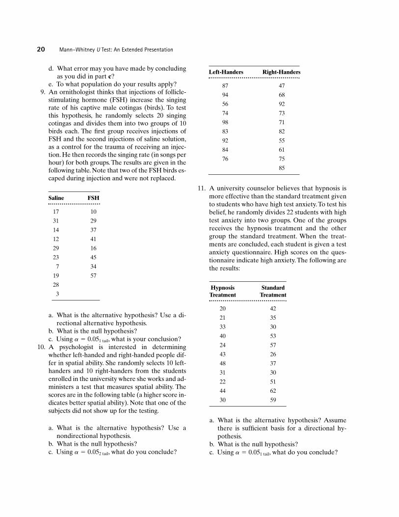
e. To what population do your results apply?9. An ornithologist thinks that injections of follicle-

stimulating hormone (FSH) increase the singingrate of his captive male cotingas (birds). To testthis hypothesis, he randomly selects 20 singingcotingas and divides them into two groups of 10birds each. The first group receives injections ofFSH and the second injections of saline solution,as a control for the trauma of receiving an injec-tion. He then records the singing rate (in songs perhour) for both groups. The results are given in thefollowing table. Note that two of the FSH birds es-caped during injection and were not replaced.

Saline FSH

17 10

31 29

14 37

12 41

29 16

23 45

7 34

19 57

28

3

a. What is the alternative hypothesis? Use a di-rectional alternative hypothesis.

b. What is the null hypothesis?c. Using � � 0.051 tail, what is your conclusion?

10. A psychologist is interested in determiningwhether left-handed and right-handed people dif-fer in spatial ability. She randomly selects 10 left-handers and 10 right-handers from the studentsenrolled in the university where she works and ad-ministers a test that measures spatial ability. Thescores are in the following table (a higher score in-dicates better spatial ability). Note that one of thesubjects did not show up for the testing.

a. What is the alternative hypothesis? Use anondirectional hypothesis.


Left-Handers Right-Handers

87 47

94 68

56 92

74 73

98 71

83 82

92 55

84 61

76 75

85

11. A university counselor believes that hypnosis ismore effective than the standard treatment givento students who have high test anxiety.To test hisbelief, he randomly divides 22 students with hightest anxiety into two groups. One of the groupsreceives the hypnosis treatment and the othergroup the standard treatment. When the treat-ments are concluded, each student is given a testanxiety questionnaire. High scores on the ques-tionnaire indicate high anxiety. The following arethe results:

Hypnosis StandardTreatment Treatment

20 42

21 35

33 30

40 53

24 57

43 26

48 37

31 30

22 51

44 62

30 59

a. What is the alternative hypothesis? Assumethere is sufficient basis for a directional hy-pothesis.


Web Connection 21

WEB CONNECTION

Go to http://psychology.wadsworth.com/courses/statistics/ and test your knowledge of this chapter by

taking the online quiz. You can also find additionalfully solved practice problems there.

NOTES

1. These probabilities could also have been calcu-lated from multiplication and addition rules. Forexample, to determine p(U � 0) such that all theC scores are lower than E scores, we need to de-termine p(CCCEEE).Assume we have a bag con-taining three C scores and three E scores and weare randomly sampling one score at a time with-out replacement. What is the probability we shallget the order CCCEEE? The solution is as fol-lows. By using the multiplication rule,

Note that each order yields the same probabilityvalue (0.05). Thus, to find the other probabilities,all we need do is multiply 0.05 by the number oforders yielding the particular U value. For exam-ple, find p(U � 2) with Cs lower than Es, since thereare two orders that yield U � 2 in this direction:

P(U � 2) � 2(0.05) � 0.10

� 36

. 25 . 14

. 33 . 22 .

11 � 0.05

p(U � 0) � p(CCCEEE)

Mann–Whitney U Test: An Extended Presentation · Mann–Whitney U Test: An Extended Presentation...

Documents

Transcript of Mann–Whitney U Test: An Extended Presentation · Mann–Whitney U Test: An Extended Presentation...