Managing Geological Uncertainty with Decision Analysis in ...
225
Managing Geological Uncertainty with Decision Analysis in Reservoir Management Probabilistic History Matching, Robust Production Optimization, and Value-of-Information by Aojie Hong Thesis submitted in fulfillment of the requirements for degree of PHILOSOPHIAE DOCTOR (PhD) Department of Petroleum Engineering Faculty of Science and Technology 2017
Transcript of Managing Geological Uncertainty with Decision Analysis in ...

Managing Geological Uncertainty with Decision Analysis in Reservoir
Management Probabilistic History Matching, Robust Production
Optimization, and Value-of-Information
by
Aojie Hong
Thesis submitted in fulfillment of the requirements for degree of PHILOSOPHIAE DOCTOR
(PhD)
Department of Petroleum Engineering Faculty of Science and Technology
2017

University of Stavanger N-4036 Stavanger NORWAY www.uis.no
©2017 Aojie Hong
ISBN: 978-82-7644-744-6
ISSN: 1890-1387
PhD Thesis UiS No. 371

i
Preface
This thesis has been written to partially fulfill the graduation requirements of the Philosophiae Doctor (PhD) degree at the Department of Petroleum Engineering, Faculty of Science and Technology, University of Stavanger, Norway. I was engaged in writing this thesis from May to October 2017.
This research was conducted under the main supervisor, Prof. Reidar B. Bratvold at the University of Stavanger and the co-supervisor, Dr. Geir Nævdal at the International Research Institute of Stavanger. It was funded by the National IOR Centre of Norway from October 2014 to October 2017. The work was conducted mainly at the University of Stavanger and partially at the University of Texas at Austin from February to July 2017.
This work intends to illustrate and discuss the implementation of decision analysis tools to manage geological and petrophysical uncertainties for better decision making in reservoir management contexts. I believe that this work will be of great interest to both managers and engineers in oil and gas companies and to scholars and researchers at academic and research institutes, who are engaged in improving the quality of oil and gas operation related decisions.
Aojie Hong
Stavanger, November 7, 2017

ii
Abstract
Reservoir management (RM) is a decision-oriented activity where decision makers use their current knowledge to search for production strategies that maximize the value of hydrocarbon production from a reservoir. Two central components of RM are history matching (HM) and production optimization (PO). HM draws on information from data. The information is then used to support decisions on production strategies. The optimal production strategy is identified through PO.
Decisions will not be good unless they account for relevant and material uncertainties in a given decision context. Uncertainty is a result of not having perfect (i.e., complete) information. Although the oil and gas industry has long been aware of the importance of uncertainty understanding and management, decision-driven approaches that include consistent uncertainty quantifications are not commonly or comprehensively used. The intent of using decision-driven approaches is to manage uncertainties for good decision making.
This work intends to address three of the main challenges of using decision analysis (DA) tools for managing geological and petrophysical uncertainties in RM. The first challenge is in describing the geological and petrophysical uncertainties using probability distributions that result from HM. The second challenge is in the computational complexity of modeling flow behaviors and solving for the optimal production strategy when given a description of geological and petrophysical uncertainties. The third challenge is in the PO approach that can allow for learning over time. The ultimate goal of this work is to illustrate and discuss how these challenges can be overcome and to facilitate the application of decision quality in RM contexts.
The first challenge is addressed through illustrating and discussing the implementation of probabilistic HM approaches. Unlike a deterministic HM approach which results in a single combination of production model parameters that best matches the given production data, a probabilistic HM approach produces numerous combinations of production model parameters, each of which has a probability, to quantify the geological and petrophysical uncertainties. Modeling with these combinations of production model

iii
parameters propagates the geological and petrophysical uncertainties to the uncertainty in future production.
The second challenge is addressed through illustrating and discussing the implementation of robust optimization (RO) algorithms and proxy production models. RO approaches identify the optimal production strategy that maximizes the expected value over many geological and petrophysical realizations. To speed up the process of solving an RO problem, we use a proxy production model to supplement a grid-based reservoir model. The proxy model captures only the most relevant physics and mechanisms affecting production prediction and thus is much more computationally attractive than the grid-based reservoir model.
The third challenge is addressed through illustrating and discussing the implementation of a fully structured reservoir management (FSRM) approach. The FSRM approach is based on the fully structured decision tree for a sequential decision-making problem in a RM context. It allows for learning over time by considering both the uncertainties associated with current available data and the uncertainties associated with future data. Therefore, the current decision does not depend only on the uncertainties that a decision maker has learned so far but on the uncertainties that the decision maker will learn in the future. The FSRM approach provides the optimal production strategy, whereas the state-of-the-art RM approach—closed loop reservoir management (CLRM)—might give a sub-optimal production strategy. Furthermore, we illustrate and discuss an a priori analysis on information valuation, known as value-of-information (VOI) analysis, in RM contexts. It evaluates the benefits of collecting additional information before one gathers the data and makes a decision. It can also be used to assess the value of accounting for learning over time in PO.
This work presents numerous examples to demonstrate the value of applying DA tools in RM. The main contribution of this work is the illustration and discussion of the implementation of decision-driven approaches for good decision making in RM contexts. To achieve this purpose, we:
1. show how to integrate model uncertainty in probabilistic decline curve analysis for unconventional oil production forecasting;

iv
2. illustrate and discuss how to use a capacitance-resistance model as a proxy model to speed up the process of robust production optimization;
3. implement a fast analysis of the optimal improved-oil-recovery start time using a two-factor production model and the least-squares Monte Carlo algorithm;
4. illustrate and discuss how to implement a robust discretization of continuous probability distributions for VOI analysis;
5. show how to apply the VOI concept for production model parameter updating through HM.
Although other challenges remain in implementing some specific approaches in a real-world setting, we believe that this work is useful in conveying to RM professionals the benefits and implementation of DA techniques, and it can be used as guidance for future research.

v
Acknowledgements
This thesis would not have been possible without the help and support from many people, to whom I owe my deepest gratitude.
Firstly, I would like to express my sincere gratitude to my supervisor, Prof. Reidar B. Bratvold, for the continuous support of my PhD study and related research. His insightful supervision and guidance helped me throughout the research and writing of this thesis. Working under his supervision is one of the best things I have experienced in my life.
My grateful thanks also go to my co-supervisor, Dr. Geir Nævdal, for his support and guidance. I appreciate highly his help in my understanding of mathematical formulations and advice on coding and programming.
I am deeply indebted to Prof. Larry W. Lake for providing me the opportunity to visit his research group at the University of Texas at Austin. His tough questions spurred me to widen my research from various perspectives. His taking good care of me made me really enjoy the stay at Austin.
I gracefully acknowledge the financial support of the National IOR Centre of Norway, the Research Council of Norway and their industry partners (ConocoPhillips, Skandinavia AS, BP Norge AS, Det Norske Oljeselskap AS, Eni Norge AS, Maersk Oil Norway AS, DONG Energy A/S, Denmark, Statoil Petroleum AS, ENGIE E&P NORGE AS, Lundin Norway AS, Halliburton AS, Schlumberger Norge AS, and Wintershall Norge AS) for my entire PhD period. My sincere thanks also go to the University of Stavanger and the Petroleum Research School of Norway for offering me the scholarship to visit the University of Texas at Austin.
I would like to thank all my colleagues at the University of Stavanger, especially my office mate, Philip Thomas, for his stimulating discussion and daily chat.
Last but not least, I would like to thank my family—my parents, wife and baby boy—for their spiritual support throughout my PhD study and my life.

vi
I would like to apologize that I could not name here all those who helped me during my PhD period or were important to the completion of this thesis and my PhD study.
Aojie Hong

vii
List of Papers
Paper I: Integrating Model Uncertainty in Probabilistic Decline Curve Analysis for Unconventional Oil Production Forecasting Hong, A.J., Bratvold, R.B., and Lake, L.W. To be submitted for publication.
This work was presented at the SPE Workshop: Petroleum Economics—Optimisation versus Growth in Uncertain Times, 27–28 September 2017, Dubai, UAE.
Paper II: Robust Production Optimization with Capacitance-Resistance Model as Precursor Hong, A.J., Bratvold, R.B., and Nævdal, G. Published in Computational Geosciences (2017), 21 (5): 1423–1442. https://doi.org/10.1007/s10596-017-9666-8
This paper was also in the proceedings of the 15th European Conference on the Mathematics of Oil Recovery (ECMOR XV), 29 August–1 September 2016, Amsterdam, the Netherlands. https://doi.org/10.3997/2214-4609.201601840
Paper III: Fast Analysis of Optimal IOR Start Time Using a Two-Factor Production Model and Least-Squares Monte Carlo Algorithm Hong, A.J., Bratvold, R.B., and Lake, L.W. To be submitted for publication.
Paper IV: Robust Discretization of Continuous Probability Distributions for Value-of-Information Analysis Bratvold, R.B., Thomas, P., Begg, S.H., and Hong, A.J. Submitted to Journal of Petroleum Science and Engineering.
This paper was also in the proceedings of the International Petroleum Technology Conference, 10–12 December 2014, Kuala Lumpur, Malaysia. https://doi.org/10.2523/IPTC-17975-MS

viii
Paper V: Value-of-Information for Model Parameter Updating through History Matching Hong, A.J., Bratvold, R.B., Thomas, P., and Hanea, R.G. Submitted to Journal of Petroleum Science and Engineering.
Similar content, titled “Value of Information from History Matching—How Much Information is Enough?” was also in the proceedings of the IOR NORWAY 2017—19th European Symposium on Improved Oil Recovery, 24–27 April 2017, Stavanger, Norway. https://doi.org/10.3997/2214-4609.201700327

ix
Contents
Preface ............................................................................................................... i
Abstract ............................................................................................................ ii
Acknowledgements ......................................................................................... v
List of Papers ................................................................................................. vii
Contents .......................................................................................................... ix
List of Figures ................................................................................................. xi
List of Tables ................................................................................................ xiii
Abbreviations ............................................................................................... xiv
Symbols ......................................................................................................... xvi
1 Introduction ............................................................................................. 1
1.1 Motivation ......................................................................................... 1
1.2 Research Goals.................................................................................. 3
1.3 Thesis Structure ................................................................................ 4
2 Managing Geological Uncertainty in History Matching ..................... 6
2.1 History Matching Approaches .......................................................... 6
2.1.1 Deterministic History Matching Approaches............................ 6
2.1.2 Probabilistic History Matching Approaches ............................. 9
2.2 Integrating Model Uncertainty in Probabilistic History Matching . 18
2.2.1 Calculating Model Probabilities Using Bayes’ Theorem ........ 19
2.2.2 Example of Application—Probabilistic Decline Curve Analysis with Multiple Models .............................................................................. 21
3 Managing Geological Uncertainty in Production Optimization ....... 24
3.1 Robust Production Optimization ..................................................... 24
3.2 Speeding up RO of Waterflooded Production Using CRM ............ 30
3.2.1 Proxy Models vs. Rich Models ............................................... 30

x
3.2.2 Proxy-model Workflow for RO .............................................. 31
3.2.3 Value of Verisimilitude ........................................................... 32
3.2.4 CRM for Waterflooding .......................................................... 33
3.2.5 Example of Applying the Proxy-model Workflow ................. 35
4 Managing Geological Uncertainty in Reservoir Management .......... 42
4.1 Closed Loop Reservoir Management .............................................. 42
4.2 Fully Structured Reservoir Management ........................................ 44
4.3 Least-Squares Monte Carlo Algorithm for FSRM .......................... 47
4.3.1 LSM Algorithm ....................................................................... 47
4.3.2 Example of Applying LSM ..................................................... 48
5 Value-of-Information in Reservoir Management .............................. 55
5.1 Definition of VOI ............................................................................ 55
5.2 VOI Calculation for Continuous Probability Distributions ............ 58
5.2.1 High Resolution Probability Tree Discretization Method ...... 58
5.2.2 Accuracy of HRPT .................................................................. 59
5.2.3 Comparison of HRPT and MC-based Methods ...................... 61
5.3 VOI Calculation for Reservoir Management .................................. 62
5.3.1 Relationship between Terms in VOI Analysis and Reservoir Management ............................................................................................ 62
5.3.2 Decision-tree Example of VOI Calculation for Reservoir Management ............................................................................................ 64
5.3.3 VOI Calculation Using Ensemble-based Methods for Reservoir Management ............................................................................................ 67
6 Overview of Research Papers .............................................................. 75
7 Summary and Conclusions ................................................................... 78
8 Discussion and Future Research .......................................................... 81
References ...................................................................................................... 83

xi
List of Figures
Figure 2.1—Moving window approach for approximating measurement error SDs. ................................................................................................................. 11 Figure 2.2—Reservoir simulation model representing the “truth.” ................ 15 Figure 2.3—The initial PermH field (in md) of an ensemble member. .......... 16 Figure 2.4—The mean over the updated ensemble of the PermH field. ......... 17 Figure 2.5—Simulation results of the initial ensemble and the updated ensemble. ........................................................................................................ 17 Figure 2.6—Synthetic dataset to day 200. ...................................................... 22 Figure 2.7—Boxplots of cumulative oil production forecasted using solely one model and using the proposed approach given the synthetic data to day 200. 23 Figure 3.1—Illustration of the 2D model and well locations.......................... 28 Figure 3.2—Three realizations of the permeability field for the 2D model. .. 28 Figure 3.3—Iterative ENPV and cumulative simulation runs. ....................... 28 Figure 3.4—Optimal injection scheme for the EnOpt example. ..................... 29 Figure 3.5—CDF of NPV under the optimal injection scheme for the EnOpt example. .......................................................................................................... 29 Figure 3.6—Traditional and proxy-model workflows for RO. ....................... 31 Figure 3.7—Schematic of (a) CRMT, (b) CRMP, and (c) CRMIP. ............... 34 Figure 3.8—Matching of total fluid production rate and water cut: (a) total fluid production rate from the 2D model, (b) water cut from the 2D model, (c) total fluid production rate from Coupled CRMP, and (d) water cut from Coupled CRMP. ............................................................................................................ 36 Figure 3.9—Validation of total fluid production rate and water cut: (a) total fluid production rate from the 2D model, (b) water cut from the 2D model, (c) total fluid production rate from Coupled CRMP, and (d) water cut from Coupled CRMP. .............................................................................................. 36 Figure 3.10—CDFs of NPV for the proxy-model workflow example. .......... 38 Figure 3.11—Optimal injection schemes for the proxy-model workflow example. .......................................................................................................... 38 Figure 3.12—Decision tree with the optimal solution of the proxy-model workflow. ........................................................................................................ 40 Figure 3.13—Decision tree with the optimal solution of the traditional workflow. ........................................................................................................ 40

xii
Figure 3.14—CDF of the VOV for the example of applying the proxy-model workflow. ........................................................................................................ 41 Figure 3.15—Sensitivity of EVOV to valve cost. .......................................... 41 Figure 4.1—Process flow of CLRM, adopted from Jansen et al. (2009). ....... 43 Figure 4.2—Decision-tree representation for CLRM. .................................... 43 Figure 4.3—Decision-tree representation of FSRM. ...................................... 44 Figure 4.4—Water cuts of R1 and R2............................................................. 45 Figure 4.5—Decision tree for the example comparing FSRM and CLRM solutions. ......................................................................................................... 46 Figure 4.6—Primary recovery as a function of time for three geological realizations. ..................................................................................................... 50 Figure 4.7—Fully structured decision tree for the example of an optimal IOR start time problem. All NPV values are in million USD................................. 51 Figure 5.1—Illustration of HRPT discretized outcomes and MC samples for a continuous probability distribution. ................................................................ 59 Figure 5.2—Average relative VOI error as a function of the number of degrees for the TALL-N problem. ............................................................................... 60 Figure 5.3—Relative error of VOI estimates using HRDT, BMC, and EnKF. ........................................................................................................................ 62 Figure 5.4—Oil production rate profiles of three realizations. ....................... 65 Figure 5.5—Uncertainty trees in (a) assessed form, and (b) inferential form. 65 Figure 5.6—Decision tree for the case with information. ............................... 66 Figure 5.7—Decision tree for the case without information........................... 66 Figure 5.8—Procedure of VOI calculation using the BvHJ approach. Adapted from Barros et al. (2016). ................................................................................ 68 Figure 5.9—Schematic of VOI calculation using MC-based methods. .......... 71 Figure 5.10—PDFs of VOI estimates of BvHJ, F1, and F2 approaches with ensemble size of 50. ........................................................................................ 73

xiii
List of Tables
Table 2.1—Loss function value of MLE for the Arps model, SEM, and Pan CRM for deterministic HM. ............................................................................ 22 Table 2.2—Statistics for cumulative oil production forecasted by the Arps model. ............................................................................................................. 22 Table 4.1—Likelihood matrix for the example comparing FSRM and CLRM solutions. ......................................................................................................... 45 Table 4.2—Injection rates for decision nodes solved using FSRM and CLRM. ........................................................................................................................ 46 Table 4.3—Likelihood functions for the measured primary recovery efficiency. ........................................................................................................................ 50 Table 4.4—Path of measured data for LSM. .................................................. 52 Table 4.5—NPVs for alternatives at time 2 for LSM. .................................... 52 Table 4.6—ENPVs for alternatives at time 2 for LSM. .................................. 52 Table 4.7—NPVs for alternatives at time 1 for LSM. .................................... 53 Table 4.8—ENPVs for alternatives at time 1 for LSM. .................................. 53 Table 4.9—NPVs for alternatives at time 0 for LSM. .................................... 54 Table 4.10—Table representation of optimal decision policy solved using LSM. ........................................................................................................................ 54 Table 5.1—Relationship between terms used in VOI analysis and those in RM. ........................................................................................................................ 63 Table 5.2—Likelihood function for the decision tree example. ..................... 65 Table 5.3—VOI estimates using BvHJ, F1, and F2 approaches with ensemble size of 10000. .................................................................................................. 73 Table 5.4—Statistics of VOI estimates of BvHJ, F1, and F2 approaches with ensemble size of 50. ........................................................................................ 73 Table 5.5—VOI estimates for the example with a reservoir simulation model. ........................................................................................................................ 74

xiv
Abbreviations
2D/3D Two Dimentional / Three Dimensional BHP Bottom Hole Pressure BMC Bayes Monte Carlo CDF Cumulative Density Function CI Confidence Interval CLRM Closed Loop Reservoir Management CRM Capacitance-Resistance Model CRMIP Injector-Producer-pair-based CRM CRMP Producer-based CRM CRMT Single Tank CRM DA Decision Analysis DM Decision Maker DWI Decision with Additional Information DWOI Decision without Additional Information EnKF Ensemble Kalman Filter EnOpt Ensemble-based Optimization ENPV Expected NPV EOR Enhanced Oil Recovery EV Expected Value EVOV Expected VOV EVWI EV with Additional Information EVWOI EV without Additional Information FOPR Field Oil Production Rate FSRM Fully Structured Reservoir Management FWCT Field Water Cut HM History Matching HRPT High Resolution Probability Tree HWS Half Window Size IOR Improved Oil Recovery LSE Least Squares Estimation LSM Least-Squares Monte Carlo MAP Maximum a Posteriori Approach MC Monte Carlo MCMC Markov-Chain Monte Carlo MCS Monte Carlo Simulation MLE Maximum Likelihood Estimation NPV Net Present Value O&G Oil and Gas

xv
OOIP Original Oil in Place PDF Probability Density Function PO Production Optimization RM Reservoir Management RO Robust Optimization SD Standard Deviation SEM Stretched Exponential Model USD US Dollar VOC Value-of-Clairvoyance VOI Value-of-Information VOPI Value-of-Perfect-Information VOV Value of Verisimilitude WBHP Well Bottom Hole Pressure

xvi
Symbols
Alternative Decision space Discount factor Covariance matrix Reference time for discounting Recovery efficiency Function Gradient matrix Water injection rate Objective function value Index of time step Kalman gain Kalman gain matrix Index of iteration Loss function value Production model Number of realizations (ensemble size) Oil Probability, or probability distribution Price Production rate Cumulative production Time, or total fluid Total number of time steps Control vector (vector of control variables) Value Water Vector of model parameters Measured data Vector of measured data Modeled data Updating step length Measurement noise/error Vector of measurement noises/errors Connectivity Standard deviation Time constant

xvii
Prior knowledge Posterior knowledge

xviii

Introduction
1
1 Introduction
1.1 Motivation The goal of an oil company is to maximize shareholder or stakeholder value by maximizing the net present value (NPV), which in turn can be maximized by minimizing capital investments and operating expenses while maximizing economic recovery of hydrocarbon from a reservoir through reservoir management (RM). Various definitions of “reservoir management” have been proposed (Haldorsen and Van Golf-Racht 1989, Robertson 1989, Wiggins and Startzman 1990, Satter et al. 1994). These definitions all emphasize that RM is a decision-oriented activity where a decision maker (DM) seeks a production strategy that maximizes the value (commonly quantified by NPV) of hydrocarbon production from a reservoir based on the DM’s current knowledge.
A common practice is to use a production model to describe the flow behaviors in a reservoir. Such a model can be a decline curve model or a reservoir simulation model. It is assumed that once the values for the model parameters have been assessed, the model itself will correctly predict future production.1 Model parameters are updated through history matching (HM), 2 and the optimal production strategy is determined through production optimization (PO) on the history-matched model. Therefore, HM and PO are the two central components of RM.
Begg et al. (2014) provided a formal definition of uncertainty— “Not knowing if a statement (or event), is true or false”—which we will use in this work. Numerous papers have shown the importance of uncertainty quantification in
1 Nobody really believes that this is the case, but it is viewed as a reasonable assumption that will yield “good enough” results. 2 In other modeling contexts, the “matching” of models to measured data is usually referred to as model calibration. We will use “history matching” and “model calibration” interchangeably. Originally, HM referred to the adjustment of production model parameters to reproduce the historical production data (rates and pressures) as closely as possible. Today, the term HM is often used in a broader context and includes model calibration using all relevant data and information (seismic data, log data, tracer behavior, etc.).

Introduction
2
forecasting. Skov (1995) concluded that the quality of the production forecast can be improved if one can quantify the range of uncertainty and obtain feedback on the accuracy of the forecast. Jonkman et al. (2010) related a company’s practices to its economic performance and found that the companies that rigorously took uncertainty into account and planned for multiple possibilities when planning for development, appeared to obtain better production forecasting and decision making, and consequently had higher economic performance. Wolff (2010) noted that it is more meaningful to generate multiple outcomes on a set of models based on uncertainties than to find a single ‘‘true’’ answer. Three comparative studies were done for the PUNQ-S3 problem (Floris et al. 2001, Barker et al. 2000, Hajizadeh et al. 2010). In these studies, uncertainty quantification methods were applied to a synthetic model. They illustrated the use of multiple history matched models for uncertainty quantification.
After fast growth in the understanding of uncertainty within the oil and gas (O&G) industry, many authors introduced the tools that can be used to capture both geological3 and non-geological uncertainties. Clarkson and McGovern (2005) presented a coalbed methane prospecting tool that integrates reservoir simulators with a reservoir model, Monte Carlo simulation, and economic modules, and an infill-well locating tool that can evaluate the locations of an infill-well by combining simulations and economics. When time constraints or a lack of reservoir data make it infeasible to forecast by full-field reservoir simulation, these two tools will be very useful. Jannink and Bos (2005) suggested a fully probabilistic methodology that is able to model both discrete and continuous uncertainties. Their work integrated the pollutant discharge forecast uncertainties and decision making of asset investment, which means that the discharge risk can be converted to financial risk. A model introduced by Morgan (2005) can be used to predict a range of oil price in both the short term and the long term, one of the biggest non-geological uncertainties in O&G economics. His model utilized the oil price data from 1986 to 2003.
Numerous authors have emphasized that it is essential that relevant and material uncertainties (no matter geological or non-geological) need to be represented by multiple realizations or scenarios for decision making. This thesis focuses
3 For brevity, this thesis uses “geological” to mean “geological and petrophysical.”

Introduction
3
on managing the geological uncertainty for making good decisions in RM contexts. 4 Non-geological uncertainty has been addressed in Thomas and Bratvold (2015), which accounted for the uncertainties in future oil and gas prices in a gas cap blowdown decision making context.
The O&G industry has long been aware of the importance of uncertainty management, but decision analysis (DA), which leverages consistent probabilistic approaches as a way to manage uncertainties for good decision making, is not commonplace in the industry because of technical and non-technical challenges. This thesis simply uses the phrase “uncertainty management” to refer to “decision-focused uncertainty management,” meaning that the intent of uncertainty management is for making good decisions, as reflected in the statement by Bratvold et al. (2009) that quantifying uncertainty has no value in and of itself and value can be created only through our decisions.
Based on our communication with many industry insiders, an example of non-technical challenges is that many people are not comfortable working with probabilities and thus refuse to use a probabilistic approach. Non-technical challenges are outside the scope of this thesis. From the technical challenges arise the following questions, which form the research problems of this thesis:
1. How can geological uncertainty in HM be managed? 2. How can geological uncertainty in PO be managed? 3. How can DA be incorporated with RM?
1.2 Research Goals Given that value can be created only through the implementation of high-quality decisions, which in turn rely on high-quality uncertainty assessments, we intend to use decision-driven approaches to manage uncertainties for good decision making. Through a literature review, we have identified three main challenges to making high-quality RM decisions:
4 A good decision is “an action we take that is logically consistent with our objectives, the alternatives we perceive, the information we have, and the preference we feel” (Bratvold and Begg 2010).

Introduction
4
1. describing geological uncertainty using probability distributions as a result of HM;
2. computational complexity of modeling flow behaviors and solving for the optimal production strategy when a description of geological uncertainty is given;
3. formulating a production optimization approach that can allow for learning over time.
The goal of this research is to illustrate and discuss how these challenges can be overcome and to facilitate the application of decision quality in RM contexts. To achieve this goal, we will address these challenges through
1. illustrating and discussing the implementation of probabilistic HM approaches, with a focus on how to integrate model uncertainty in probabilistic decline curve analysis for unconventional oil production forecasting;
2. illustrating and discussing the implementation of robust optimization (RO) algorithms and proxy production models, with a focus on how to use a proxy model to speed up the process of robust production optimization;
3. illustrating and discussing the implementation of the fully structured reservoir management (FSRM) approach, with focuses on how to use a two-factor production model and the least-squares Monte Carlo (LSM) algorithm for fast analysis of optimal improved-oil-recovery (IOR) start time and on how to apply the value-of-information (VOI) concept for production model parameter updating through HM.
We are concerned with providing good approaches to manage uncertainties for good decision making. A good approach must be both useful and tractable. By “useful,” we mean “providing clear insight for decision making” and by “tractable,” we mean that the analysis can be done with the time and resources available.
1.3 Thesis Structure This thesis is structured in the form of paper collection, with two parts. The first part is an introduction summarizing the research and clarifying how the topics

Introduction
5
of the included papers are interrelated. The second part consists of 5 papers which have been published or submitted, or will be submitted for journal publications.
The reminder of the thesis is divided into the following chapters:
Chapter 2 reviews deterministic and probabilistic HM approaches and introduces an approach to integrate model uncertainty in probabilistic HM using the moving window approach and minimum likelihood estimation (MLE);
Chapter 3 reviews RO with the ensemble-based optimization (EnOpt) algorithm and proposes a workflow of using a capacitance-resistance model (CRM) to speed up the RO process for waterflooded production;
Chapter 4 reviews the state-of-the-art reservoir management tool—closed loop reservoir management (CLRM), discusses how it will improve decision making, and compares it with FSRM;
Chapter 5 reviews the concept of VOI, which can be used to value the information in an RM context, and presents a workflow of assessing it using state-of-the-art HM and PO tools;
Chapter 6 provides an overview of the research papers included in the second part of the thesis;
Chapter 7 summarizes and concludes this research; Chapter 8 presents a discussion and suggestions for future research.

Managing Geological Uncertainty in History Matching
6
2 Managing Geological Uncertainty in History Matching
The purpose of a production model (a decline curve model, a reservoir simulation model, etc.) is to predict future production for our decisions on production strategy. Thus, the quality of a production model can affect our choice of the optimal production strategy. The quality of a production model means the similarity of the predicted production to the real production. This in turn relies on the similarity of the geological properties described by the model and its corresponding parameters to the real geological properties of a field. The higher similarity the model has, the higher quality the model has.
A production model is mathematically formulated based on our understanding of the underlying physical principles. Its parameters are based on our knowledge of the geological properties of a field. This knowledge comes from information provided by seismic data, core data, well log data, production data and so on. Our research focuses on the information provided by production data. The parameter settings of a production model are usually determined through an HM process where the model parameters are tuned such that it can closely reproduce historical production. The goal of HM is to correctly forecast production so that the forecast can be used for decision making.
However, the data we can access today represent only a part of the reservoir, and we can never know the subsurface in all its detail. Thus, geological uncertainties always exist in a production model, although HM can reduce the uncertainties. Because of the uncertainties, a more realistic goal of HM is to quantify our lack of knowledge (i.e., to quantify our uncertainty) about the future production, for the purpose of making good decisions.
2.1 History Matching Approaches
2.1.1 Deterministic History Matching Approaches In a deterministic world, the goal is to identify the true nature of the relevant parameters of a given model. We do this by applying HM, which is an

Managing Geological Uncertainty in History Matching
7
optimization process where the objective function is a predefined loss function that we seek to minimize by tuning the model parameters. The model with its parameter settings which minimizes the loss function is referred as the best fit model.
2.1.1.1 Least Squares Estimation
An extensively used HM approach is least squares estimation (LSE) where the loss function is defined as the squared difference between model forecast and data:
(2.1)
where is the loss function of LSE which is a function of the vector of model parameters , is the model forecasted production at time step ,
is the measured production (i.e., the data) at time step , and is the total number of time steps of data.
2.1.1.2 Maximum Likelihood Estimation
Another approach is maximum likelihood estimation (MLE), which aims to maximize the likelihood function (i.e., the probability of observing the data given a set of model parameter settings). Assuming that the data measurements are independent, we can define the likelihood function as
(2.2)
where denotes probability, and denotes the conditional probability of measured data given parameters . Applying a Gaussian random error for the measurement with zero mean and standard deviation (SD) , we obtain
(2.3)
Managing Geological Uncertainty in History Matching
8
Thus,
(2.4)
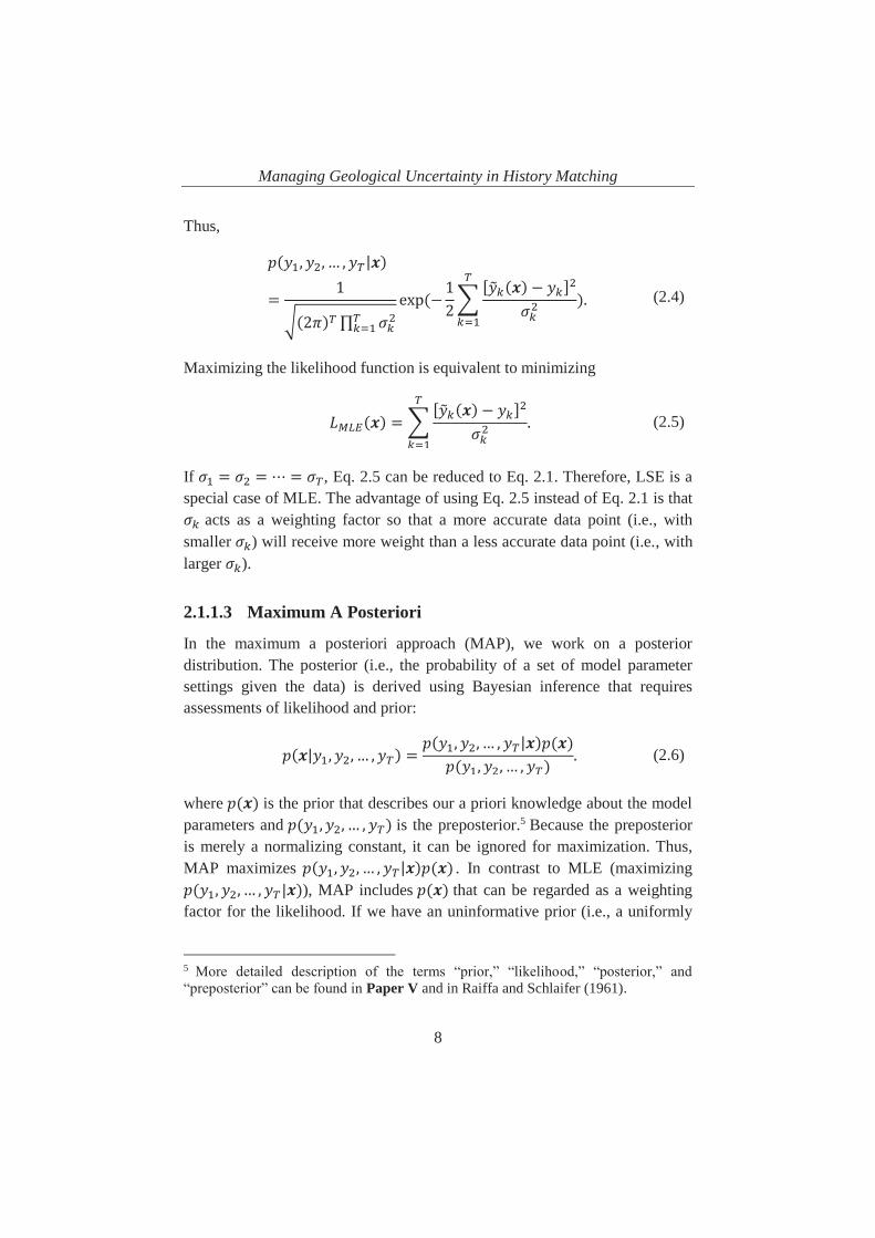
Maximizing the likelihood function is equivalent to minimizing
(2.5)
If , Eq. 2.5 can be reduced to Eq. 2.1. Therefore, LSE is a special case of MLE. The advantage of using Eq. 2.5 instead of Eq. 2.1 is that
acts as a weighting factor so that a more accurate data point (i.e., with smaller ) will receive more weight than a less accurate data point (i.e., with larger ).
2.1.1.3 Maximum A Posteriori
In the maximum a posteriori approach (MAP), we work on a posterior distribution. The posterior (i.e., the probability of a set of model parameter settings given the data) is derived using Bayesian inference that requires assessments of likelihood and prior:
(2.6)
where is the prior that describes our a priori knowledge about the model parameters and is the preposterior.5 Because the preposterior is merely a normalizing constant, it can be ignored for maximization. Thus, MAP maximizes . In contrast to MLE (maximizing
), MAP includes that can be regarded as a weighting factor for the likelihood. If we have an uninformative prior (i.e., a uniformly
5 More detailed description of the terms “prior,” “likelihood,” “posterior,” and “preposterior” can be found in Paper V and in Raiffa and Schlaifer (1961).

Managing Geological Uncertainty in History Matching
9
distributed prior), is independent of the value of and is constant. In such case, maximizing is equivalent to maximizing
. Therefore, MLE is a special case of MAP.
We have shown that LSE, MLE, and MAP are related to each other and all based on Bayes’ theorem. Although probabilities are considered, these approaches give a single estimate rather than a distribution, which precludes uncertainties from being included in further analysis.
2.1.2 Probabilistic History Matching Approaches In HM, uncertainties come from measurement (or observational) errors, non-uniqueness of inverse modeling, and the production model itself. By “measurement error,” we mean the difference between a measured value of a quantity and its true value. It describes the inherent variability in the results of a measurement process. By “non-uniqueness of inverse modeling,” we mean that multiple good fits to the data can be obtained with various combinations of model parameter settings. The third source of uncertainty (the production model) will be discussed in detail in Section 2.2. For now, the production model is a given. The mentioned uncertainties should be reflected by the model parameters with their distributions.
2.1.2.1 Non-uniqueness in Inverse Modeling
Tavassoli et al. (2004) presented the issue of non-uniqueness in inverse modeling (which they called the inherent uncertainty in HM) and demonstrated that different combinations of model parameter values, which give almost equally good HM results, can give different forecasts. To address this, Sayarpour et al. (2011) started with different sets of initial guesses of model parameters to history match data to generate numerous history matched solutions of model parameters. This approach provides a probability distribution that reflects the non-uniqueness issue, and it is applied in Paper I.
2.1.2.2 Bootstrap Method
Cheng et al. (2010) and Jochen and Spivey (1996) used the bootstrap method to incorporate measurement errors in HM. The bootstrap method is a type of
Managing Geological Uncertainty in History Matching
10
Monte Carlo (MC) method for approximate Bayesian inference (Hastie et al. 2009) and assumes non-informative prior. The bootstrap method is applied through the following procedure:
1) Generate a sampled dataset by resampling data points from the original dataset with replacement;
2) Use LSE to history match the sampled dataset to obtain a set of model parameter settings;
3) Repeat Steps 1 and 2 numerous times to obtain numerous sets of model parameter values;
4) Use these sets of model parameter values as MC samples representing the distributions of the model parameters.
The bootstrap method does not require that explicit distributions be assigned to the measurement errors because they are approximated by the perturbed data (Hastie et al. 2009).
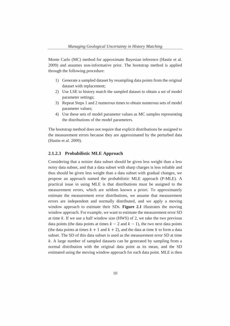
2.1.2.3 Probabilistic MLE Approach
Considering that a noisier data subset should be given less weight than a less noisy data subset, and that a data subset with sharp charges is less reliable and thus should be given less weight than a data subset with gradual changes, we propose an approach named the probabilistic MLE approach (P-MLE). A practical issue in using MLE is that distributions must be assigned to the measurement errors, which are seldom known a priori. To approximately estimate the measurement error distributions, we assume that measurement errors are independent and normally distributed, and we apply a moving window approach to estimate their SDs. Figure 2.1 illustrates the moving window approach. For example, we want to estimate the measurement error SD at time . If we use a half window size (HWS) of 2, we take the two previous data points (the data points at times and ), the two next data points (the data points at times and ), and the data at time to form a data subset. The SD of this data subset is used as the measurement error SD at time
. A large number of sampled datasets can be generated by sampling from a normal distribution with the original data point as its mean, and the SD estimated using the moving window approach for each data point. MLE is then

Managing Geological Uncertainty in History Matching
11
used to history match each sampled dataset, yielding many sets of model parameter settings. This proposed approach is applied in Paper I.
Figure 2.1—Moving window approach for approximating measurement error SDs.
2.1.2.4 Ensemble Kalman Filter
When a priori knowledge is considered, a fully Bayesian approach should be used. Approaches for Bayesian HM include the ensemble Kalman filter (EnKF) and Markov-chain Monte Carlo (MCMC). The present work applies EnKF because it is easily implemented with any production model, it is computationally attractive, and it can handle large datasets and a considerable number of model parameters. The first use of EnKF in petroleum engineering is probably that described by Lorentzen et al. (2001). Following its publication, this method attracted significant attention, and the number of papers applying and discussing EnKF increased rapidly.
The following briefly reviews EnKF. For a comprehensive introduction to EnKF, see Evensen (2009). Aanonsen et al. (2009) provided an extensive review of the application of EnKF in reservoir engineering.
2.1.2.4.1 EnKF Formulation
The basic idea behind EnKF is based on the Kalman (1960) filter. The Kalman filter is a solution to estimating the state6 of a process in a recursive way and is 6 Given a dynamic system, a state is an unobservable (in most cases) quantity that is required, and thus must be determined, to predict the system behavior (i.e., the future state). A state can be a scalar or a vector.

Managing Geological Uncertainty in History Matching
12
designed for linear filtering and prediction problems with discrete data. This method seeks an optimal weight between measured data and model forecast. Normal distribution is used to describe an uncertain quantity, say the production rate , at a certain time: the forecasted by a model is normally distributed
, where is the model forecasted mean and is the SD of model forecast, and the measured by a device is normally distributed , where is the measured mean and is the SD of measurement error. A linear combination of the model forecast and measured data can be constructed as
(2.7)
where is the updated estimate of given measured data, and (the Kalman gain) is a weighting factor for the model forecast versus the measured data. is also normally distributed , where is the updated mean and is the updated SD. Given Eq. 2.7, and
can be calculated, respectively,
(2.8) (2.9)
If we consider the best estimate as the one with the smallest SD, is minimized by adjusting , yielding
(2.10)
Replacing in Eqs. 2.8 and 2.9 with , we obtain the mean and SD of a normal distribution for the updated estimate.
Another way to obtain Eqs. 2.8, 2.9, and 2.10 is to start with Bayes’ theorem:
(2.11)
Using the properties of conjugate normal distributions, we can obtain

Managing Geological Uncertainty in History Matching
13
(2.12)
and
(2.13)
Eq. 2.12 and Eq. 2.13 can be rewritten as Eqs. 2.8 and 2.9, respectively. Using the Kalman filter, Bayesian inference is implicitly conducted.
Evensen (1994) introduced EnKF as a MC representation7 of the Kalman filter. The prior distribution is represented by a set of realizations of model parameters (i.e., the prior or initial ensemble). The posterior distribution is represented by the updated realizations of model parameters (i.e., the posterior or updated ensemble), which are obtained by (Burgers et al. 1998)
(2.14)
where matrix consists of the vectors containing the updated states, updated model parameters, and updated observations corresponding to each realization in the posterior ensemble; matrix contains the predicted states by forward modeling, model parameters, and predicted observations by forward modelling corresponding to each realization in the prior ensemble; is the Kalman gain matrix, which weighs the influences of the prior predicted observations and the real-time observations (i.e., measured data); is a matrix containing the perturbed observations;8 and is an operator that links to the predicted observations. As does Eq. 2.7, Eq. 2.14 describes a linear combination of the prior and the observations. The weighing factor is calculated as
(2.15)
7 By “MC representation” we mean that a probability distribution is represented by its corresponding MC samples. 8 When the EnKF is applied, an observation has to be perturbed with its corresponding statistics in order to avoid insufficient variance (Burgers et al. 1998).

Managing Geological Uncertainty in History Matching
14
where is the covariance matrix of encoding the covariance matrix of the prior predicted observations, and is the covariance matrix of the observations. As the measurements become noisier (i.e., the variance of an observation increases) or the variance of a prior predicted observation decreases, more weight is given to the prior; otherwise, more weight is given to the observations.
EnKF embodies the prior in , the likelihood in (when the model noise is ignored), and the posterior in ; and the preposterior is a normalizing constant of the posterior. Thus, Bayes’ rule describing the relationship among the prior, the likelihood, the preposterior, and the posterior is no longer shown explicitly as in Eq. 2.11, but is implicit in Eqs. 2.14 and 2.15. Using EnKF in the context of HM requires the initial guess of the model parameters (i.e., the prior ensemble) together with a model that can predict both the production and observations given a production strategy, observations, and their associated statistics; and the result is the EnKF updated model parameters (i.e., the posterior ensemble).
To perform Bayesian inference using EnKF requires only a few matrix operations. Thus, it is very useful for updating a reservoir simulation model which usually has thousands of parameters for determination. EnKF is applied in Paper V.
2.1.2.4.2 Example of EnKF Application
Here is an example to illustrate the application of EnKF. A 2D, horizontal, two-phase (water and black oil) reservoir simulation model is built to represent the “truth.” A horizontal injector penetrates along the left edge of the reservoir, and a horizontal producer along the right edge. For simplicity, the horizontal injector and the horizontal producer are represented by 10 vertical dummy injectors and 10 vertical dummy producers, respectively. The fluid injection rate is fixed at 15 sm3/day in each dummy injector. The production rate in each dummy producer is constrained by an upper bound of 15 sm3/day. Two highly permeable regions, with horizontal permeability of 1500 millidarcy (md), are used to mimic the water channels; and the horizontal permeability in the background is 250 md. The geometry of the model, the horizontal permeability field, and the dummy vertical wells are shown in Figure 2.2. The grid blocks

Managing Geological Uncertainty in History Matching
15
are cubic with length, width, and height equal to 10 m. The reservoir model is 450 m × 450 m × 10 m which scales to 45 blocks × 45 blocks × 1 block.
Figure 2.2—Reservoir simulation model representing the “truth.”
The unknown is the horizontal permeability (PermH) at each grid block, which means 2025 parameters for the entire grid. The base 10 logarithms of the permeabilities are used as the model parameters in EnKF because grid block permeability is usually assumed to be lognormally distributed and the use of logarithm can prevent the updated permeability calculated by EnKF from being negative. The state variables are the grid block pressures and the grid block water saturations. The true observations are the well bottom hole pressures (WBHPs) and oil production rates in all the dummy wells, obtained by running simulation on the true model. The predicted observations (WBHPs and well oil production rates) are obtained by running simulations with the updated model and state variables. Observations are recorded every 50 simulated days over a 1000-day production period, totaling 20 data points. EnKF is implemented in MATLABTM (2014), and the production model is an ECLIPSETM (2014) simulation model, so an interface between MATLAB and ECLIPSE is constructed: the updated permeabilities calculated in MATLAB are written into the input files (the .DATA-files) of ECLIPSE, the forecasted and updated pressures and saturations are read from and written into the restart files (the X-files) of ECLIPSE, respectively, the predicted observations are read from the summary files (the S-files) of ECLIPSE, and the ECLIPSE simulator can be called to run in MATLAB. The standard EnKF algorithm (Eqs. 2.14 and 2.15) is used to calculate the updated model variables (PermH) and state variables (pressures and saturations).
Initial ensemble members of the PermH field are generated by sampling from a predefined multivariate normal distribution that describes our a priori

Managing Geological Uncertainty in History Matching
16
knowledge about the PermH field. One of the initial ensemble members is shown in Figure 2.3.
Figure 2.3—The initial PermH field (in md) of an ensemble member.
To avoid physically impossible PermH values, we truncate the permeability values so that they are limited to a range (from 100 to 2500 md in this example). We do the same for the updated saturations and pressures, such that the saturations are always between 0 and 1 and the pressures are always positive.
Observations are perturbed by adding an error term drawn from a predefined normal distribution that describes our a priori knowledge about the measurement errors. In this example, we assign relatively small errors (a SD of 1 bar for all the pressure measurements and a SD of 1 sm3/day for all the oil rate measurements). In a more realistic case, the measurement errors can be much larger.
The mean over the updated ensemble of the PermH field is illustrated in Figure 2.4. Two high permeable channels similar to those illustrated in Figure 2.2 appear after applying the EnKF. The simulated results, WBHP for Producer 5 and Injector 5, field water cut (FWCT), and field oil production rate (FOPR), are shown in Figure 2.5. The grey lines represent the results generated using the initial ensemble. The cyan lines represent the results generated using the updated ensemble members. The black dashed line represents the result generated using the mean over the updated ensemble as shown in Figure 2.4. The red line represents the result generated using the true model. The measured WBHP from Producer 5, Injector 5, and measured FOPR are the red circles in Figure 2.5(a), (b), and (d), respectively. The results show that the use of EnKF not only reduces the spread of the initial ensemble (i.e., reduces the uncertainty)

Managing Geological Uncertainty in History Matching
17
but produces a good match to the measured data. A significant impact of using EnKF can be seen in Figure 2.5(c): none of the initial ensemble members predicts the water breakthrough time correctly, whereas the updated ensemble provides a nearly perfect match.
Figure 2.4—The mean over the updated ensemble of the PermH field.
(a) Producer 5: WBHP [bars] vs. Time [days] (b) Injector 5: WBHP [bars] vs. Time [days]
(c) FWCT [-] vs. Time [days] (d) FOPR [sm3/day] vs. Time [days]
Figure 2.5—Simulation results of the initial ensemble and the updated ensemble.

Managing Geological Uncertainty in History Matching
18
The updated results (the cyan lines) do not capture the truth (the red line). This does not mean that based on the updated results, the probability of the truth is zero. Recall that the EnKF uses MC samples to represent a probability distribution. The values on the cyan lines at a certain time are MC samples representing a Gaussian distribution. This underlying Gaussian distribution captures the truth.
2.2 Integrating Model Uncertainty in Probabilistic History Matching
The probabilistic HM approaches presented earlier incorporate measurement errors and non-uniqueness of inverse modeling and produce multiple realizations of model parameters to reflect these uncertainties. However, all of them assume a mathematical model that can “correctly” predict reservoir performance. The uncertainty is only in the model parameters and not in the model. This, of course, is never the case because “all models are wrong but some are useful” (Box 1979).
In this section, the context is the use of decline curve analysis for unconventional plays. Although numerical techniques for forecasting hydrocarbon production have developed rapidly over the past decades, the decline curve analysis technique is still used extensively in the O&G industry. A decline curve model is computationally attractive, and only production data that can be easily acquired is required for determining the model parameter values through the HM process. The history matched model is further used for forecasting hydrocarbon production and reserves.
One of the most extensively used decline curve models is the Arps (1945) model. However, the Arps model is often not ideal for unconventional plays (Joshi and Lee 2013). Several decline curve models have been developed in order to capture the flow behaviors in an unconventional well; for example, the power law exponential model (Ilk et al. 2008), the stretched exponential model (SEM) (Valko and Lee 2010), the Duong (2011) model, the logistic growth model (Clark et al. 2011), and the Pan (2016) CRM.
Given these models, a question arises that has not been discussed widely: which is the best model? This question seems trite because the meaning of “best” is

Managing Geological Uncertainty in History Matching
19
not well defined. In traditional practices, the model that can best fit the data in a least squares sense is regarded as the best model. However, this ignores two facts: the best fit model might not be the model that best describes the flow behaviors, and there might be several models that fit the data almost equally well.
2.2.1 Calculating Model Probabilities Using Bayes’ Theorem
Instead of identifying the “best” decline curve model for unconventional plays, we propose to regard any model as potentially good, where goodness is characterized by a probability. If a model has higher probability than the others, we say that this model is more likely to be a good model. If several models have close probabilities, we say that the model uncertainty is high because it is difficult to tell which model is more likely to be a good model.
In this manner, the model uncertainty can be easily integrated in probabilistic decline curve analysis, using the probabilistic HM approaches presented in Section 2.1.2. However, the P-MLE approach (Section 2.1.2.3) will be used here for the following reasons:
Data points should be weighted differently according to their noisiness, and distributions of measurement errors need to be assigned for calculating the model probabilities; thus, the Bootstrap method is not used.
The parameters of different models have different physical meanings and are related to the reservoir property. It is not easy to assign distributions to the parameters of different models to represent the same reservoir property based on our a priori knowledge. To compare different models fairly, it would be better to assume an uninformative prior. Therefore, a fully Bayesian approach like the EnKF, which requires an informative prior, is not used.
Consider a given dataset where is the oil production rate measured at time . The procedure to quantify the model uncertainty is

Managing Geological Uncertainty in History Matching
20
1) Estimate , which is the SD of the normal random error of the measurement of , using the moving window approach.
2) Draw an MC sample from a normal distribution with mean and SD , and repeat it for each data point to obtain a sampled dataset.
3) For a given sample dataset, use MLE to determine the parameters of each model under consideration.
4) Calculate the probability of each model with its MLE parameters, given the sampled dataset.
5) Repeat Steps 2–4 times, where is the total number of MC iterations (we use ).
6) Calculate the posterior probability of each model.
In Step 4, the probability of each model with its MLE parameters, given the sampled dataset, is calculated using Bayes’ theorem:
(2.16)
where denotes the MLE parameters of model given sampled dataset ; denotes a priori knowledge; and denotes a posteriori knowledge given . Applying a noninformative prior, we have
, reducing Eq. 2.16 to
(2.17)
Inserting Eqs. 2.4 and 2.5 (MLE loss function) into Eq. 2.17, we obtain
(2.18)
Because is a MC sample, and

Managing Geological Uncertainty in History Matching
21
(2.19)
The probability calculated using Eq. 2.19 is the probability of the estimate of interest (e.g., reserves) forecasted by model with its parameters . By repeating this process over different models and different sampled datasets, we obtain the distribution of interest, which includes uncertainties in measurements, inverse modelling and models. The posterior probability of a model in Step 6 is calculated as
(2.20)
2.2.2 Example of Application—Probabilistic Decline Curve Analysis with Multiple Models
We use an example to illustrate the impacts of using a deterministic approach or probabilistic approach without considering the model uncertainty on decline curve analysis, and to highlight the importance of integrating the model uncertainty. This example considers only three models—the Arps model, SEM, and Pan CRM—but other models can be easily added.
The “true” decline is generated using the Pan CRM. Random errors are added to the “true” decline to form the synthetic dataset. Figure 2.6 illustrates the synthetic dataset and the “true” decline of oil production rate as well as the SDs of measurement errors assessed using the moving window approach with an HWS of 10 data points. Our interest is the cumulative oil production from day 200 to day 10950 (year 30). The “true” cumulative oil production given by the Pan CRM is 48.1 Mbbl. This value is used as a reference for the estimates.
We first use a deterministic approach to estimate the cumulative oil production. The resulting loss function value of MLE for each model is listed in Table 2.1. Because the Arps model best fits the data (minimum loss function value), it is used for forecasting, providing an estimated cumulative oil production of 132.6 Mbbl. This estimate is more than 2.5 times the “true” value.

Managing Geological Uncertainty in History Matching
22
Figure 2.6—Synthetic dataset to day 200.
Arps Model SEM Pan CRM 171.65 171.75 172.29
Table 2.1—Loss function value of MLE for the Arps model, SEM, and Pan CRM for deterministic HM.
To produce a distribution of the cumulative oil production, we use the P-MLE approach with only the Arps model. The P10, P50, mean, and P90 values are listed in Table 2.2. The forecast of the Arps model is biased far from the “truth” (48.1 Mbbl), and the 80% confidence interval (CI), from P10 to P90, does not cover the “truth.”
Statistic P10 P50 Mean P90 Cumulative Oil
Production [Mbbl] 73.5 132.3 135.7 207.2
Table 2.2—Statistics for cumulative oil production forecasted by the Arps model.
We now integrate the model uncertainty in the P-MLE approach for this analysis. Table 2.1 shows that the minimized loss function values of the three models are indeed very close. Using Eq. 2.18 to convert these loss function values to probabilities, the posterior probabilities of Arps model, SEM and Pan CRM are 36.4%, 34.0%, and 29.6%, respectively. This suggests that the models are almost equally likely to be good, given the dataset. This result seems counter-intuitive as the correct model (the Pan CRM) is the least likely one.

Managing Geological Uncertainty in History Matching
23
This is because the dataset does not provide enough information to identify the correct model. Thus, the model uncertainty remains large even when the dataset is given. Figure 2.7 shows the boxplots of cumulative oil production forecasted using solely the Arps model, SEM, or Pan CRM, and using our proposed approach. Among the three models, the Arps model has the largest uncertainty in inverse modelling, as it gives the largest 80% CI, whereas the Pan CRM has the smallest uncertainty in inverse modelling. Since the Pan CRM is the correct model, its estimate is the best. Using our proposed approach, the “truth” is covered in the 80% CI. This means that by integrating the model uncertainty in the analysis, we can reduce the risk of selecting a poor model for forecasting.
Figure 2.7—Boxplots of cumulative oil production forecasted using solely one model and
using the proposed approach given the synthetic data to day 200.
The application of the proposed approaches for probabilistic decline curve analysis for unconventional wells in two fields is illustrated and discussed in Paper I.

Managing Geological Uncertainty in Production Optimization
24
3 Managing Geological Uncertainty in Production Optimization
PO is a powerful approach to design a production strategy. The goal of PO is to maximize hydrocarbon production by adjusting the control (or decision) variables (e.g., water injection rates and producer WBHPs). However, this can be expressed in different ways, such as to minimize the water cut of a producer, to optimize the WBHP of an injector, or to maximize the economic value over the life of a reservoir. This work defines the objective of PO as, to maximize NPV. The context in this work is waterflooding, and we assume that all revenues stem from oil production and that all costs are induced by water injection and water production. Thus, the objective function for a deterministic case, where a single realization is considered, is defined as
(3.1)
where is the control vector (i.e., a vector of control variables) defined as , where is the number of control variables; is the field oil
production rate at time ; is the field water production rate at time ; is the field water injection rate at time ; is the oil price; is the water production cost; and is the water injection cost; is the discount factor; is the cumulative time for discounting; and is the reference time for discounting ( = 365 days if is expressed as a fraction per year and the cash flow is discounted daily). , , and are forecasted by a given production model.
3.1 Robust Production Optimization RO of production is performed over an ensemble of realizations representing the geological uncertainty. For a risk-neutral decision maker, the objective of RO is to maximize the expected value (EV) over the ensemble,

Managing Geological Uncertainty in Production Optimization
25
(3.2)
where is the EV over all realizations (i.e., the objective function for a probabilistic case), is the objective function (Eq. 3.1) for a deterministic case with a single realization , and is the number of realizations (i.e., ensemble size).
Maximizing Eq. 3.2 can be done iteratively using the steepest ascent method. For each iteration, the control vector is updated as
(3.3)
where the subscript denotes the iteration number, is the currently updated control vector, is the previously updated control vector, is the step length for updating, and is the gradient for updating the control variables. Several methods have been proposed to estimate for each iteration. Nævdal et al. (2006) used an adjoint method to calculate . However, deriving the adjoint equation requires access to the mathematical formulation of a production model, which is impossible for commercial reservoir simulators, such as ECLIPSE that is used in this work. Chen et al. (2009) proposed the ensemble-based optimization method (EnOpt), to calculate . The EnOpt treats a production model as a black box (i.e., no requirement for its mathematical formulation) and thus can be easily implemented with any type of production model. Besides, EnOpt is specially designed for the case where an ensemble of realizations is involved, so it can significantly reduce the number of simulations required for gradient calculation. Thus, we use EnOpt for this work, as discussed in Papers II and V.
In the original EnOpt proposed by Chen et al. (2009), the ensemble of values for control vector , , …, , where is the ensemble size,9 is generated from a multivariate normal distribution with predefined mean and predefined covariance matrix , which is used to specify the temporal correlation of the
9 if each realization is coupled with one sample of values for the control vector (i.e., a 1:1 ratio is applied), as in this work.

Managing Geological Uncertainty in Production Optimization
26
controls to limit the frequency of changes to the controls. The predefined mean can be approximated by its sample mean , i.e.,
(3.4)
and the average objective value can be approximated by
(3.5)
Chen et al. (2009) used the approximation in Eq. 3.4 to calculate the mean-shifted ensemble matrix and the approximation in Eq. 3.5 to calculate the mean-shifted objective function vector . However, Do and Reynolds (2013) did not find any advantage, theoretical or practical, in approximating these two terms. Hence, they calculate the mean-shifted ensemble matrix directly using the predefined mean by
(3.6)
Moreover, Fonseca et al. (2014) suggested calculating the mean-shifted objective function vector with respect to the objective value of the predefined mean for each individual realization instead of the average objective value (Eq. 3.5), i.e.,
(3.7)
The cross-covariance matrix is then
(3.8)
Chen et al. (2009) approximated the gradient by
(3.9)
Eqs. 3.6–3.9 and 3.3 constitute the modified EnOpt formulation. The original EnOpt formulation can be obtained by replacing with in Eq. 3.6 and with the approximated in Eq. 3.7. Fonseca et al. (2014) showed that the

Managing Geological Uncertainty in Production Optimization
27
modified EnOpt converges to a higher objective value and more quickly than does the original EnOpt. Therefore, we use the modified EnOpt.
The step length significantly affects the rate of convergence. A naive line search procedure is to simply reduce by half if . The present work uses an interpolation-based line search procedure to find a relatively large value of that satisfies the Armijo condition (Wright and Nocedal 1999). The line search procedure halts when or a maximum number of iterations is reached, whichever comes first.
The stopping criterion of the iteration of the steepest ascent method is usually that the increase in the objective function value is smaller than a user-defined threshold value or a maximum number of iterations is reached, whichever comes first. In our use of EnOpt, an optimal solution is usually found during the first 5–15 iterations. In order to observe clear evidence of convergence, our stopping criterion is that the number of iterations has reached 30, which is about twice as many as have been required based on our experience.
We use a synthetic 2D reservoir model (the 2D model) to illustrate the application of the EnOpt. The 2D Model is an isotropic heterogeneous model with four injectors and one producer in a five-spot pattern. The heterogeneity pertains to permeability only. Figure 3.1 shows the geometry of the 2D model and well locations. The color map in Figure 3.1 shows a realization of the permeability field in md. The producer bottom hole pressures (BHPs) are fixed at 200 bars. The well injection rate is controllable and constrained from 0 to 200 m3/day. The control variables are injection rates for 50 time intervals of 30 days each (i.e., a life-cycle of 1500 days). For simplicity, the injection rates of all injectors for a given day are assumed to be identical. Thus, there are 50 control variables. To incorporate permeability uncertainty, we generate 100 realizations of the permeability field from a multivariate normal distribution. Three of these realizations are shown in Figure 3.2. NPV calculation uses the oil price 315 $/m3, water production cost 47.5 $/m3, water injection cost 12.5 $/m3, and discount rate 8%.
For robust production optimization, we use the modified EnOpt to maximize the expected NPV (ENPV) over all the realizations under a single injection

Managing Geological Uncertainty in Production Optimization
28
scheme. The starting point (the base case) uses an injection rate of 100 m3/day for all the producers and time steps.
Figure 3.1—Illustration of the 2D model and well locations.
Figure 3.2—Three realizations of the permeability field for the 2D model.
Figure 3.3—Iterative ENPV and cumulative simulation runs.
The ENPV and cumulative simulation runs of each EnOpt iteration are shown in Figure 3.3. The ENPV increases sharply at the beginning and starts to

Managing Geological Uncertainty in Production Optimization
29
converge after 7 iterations. The ENPV decreases at some iterations because the maximum number of line search iterations (set to 7 in this example) was reached. The optimal ENPV is $32.03 million, corresponding to an improvement of 35.59% over the base case ENPV of $23.62 million. The total number of simulation runs is 15700 for 30 iterations.
Figure 3.4 illustrates the optimal injection scheme. Its major trend is that the injection rate decreases. Because of the discounting nature of NPV calculation, the more oil produced at the early times, the better. At late times, the water cut is high, so water injection rate is reduced to a sufficient rate for continuing production.
Figure 3.4—Optimal injection scheme for the EnOpt example.
Figure 3.5—CDF of NPV under the optimal injection scheme for the EnOpt example.

Managing Geological Uncertainty in Production Optimization
30
The cumulative density function (CDF) of NPVs corresponding to the optimal injection scheme on the 2D model with the 100 realizations is illustrated in Figure 3.5. The 80% CI, from P10 to P90, is from $30.07 million to $33.61 million. The SD is $1.29 million, an order of magnitude smaller than the EV. The distribution is quite symmetric.
3.2 Speeding up RO of Waterflooded Production Using CRM
Although EnOpt has significantly reduced the number of simulation runs required, RO can still be computationally intensive when based on grid-based reservoir models using hundreds of realizations. This section presents an RO workflow that embeds proxy models for further reduction of the computational cost for RO.
3.2.1 Proxy Models vs. Rich Models Whether using rich10 models or proxy models, one should keep in mind the counsel of Box (1979), “All models are wrong but some are useful.”
Engineering uses models to support decision making. Good decision models are both useful and tractable. By “useful,” we mean that the model must be relevant and generate insight to resolve the decisions at hand. Usefulness also requires the model to be credible and transparent—will the DMs believe the result of the analysis and can the approach be clearly explained and understood? By “tractable,” we mean that the required analysis can be done within the time and resources available.
Both grid-based models and proxy models can be useful. However, a reservoir simulator such as ECLIPSE, with its voluminous code, is so feature rich and detail oriented that it is not transparent to most users. Furthermore, a rich and computationally intensive grid-based model is often not tractable—particularly when the underlying problem is uncertain.
10 We use “rich” interchangeably with “complex” and “verisimilar” to indicate a high level of detail built into a model.

Managing Geological Uncertainty in Production Optimization
31
Decision-making contexts require cogent (compelling) models. Companies tend to build too much detail into their decision-making models from the start and focus too much energy on specific cases or inputs that do not influence the decisions at hand. As stated by Bickel and Bratvold (2008), “This level of modeling detail is really a shirking of responsibility on the part of the decision analyst who will and can build a model that includes only the most salient factors. Building in detail is easy. Building in incisiveness is hard work.”
3.2.2 Proxy-model Workflow for RO When geological uncertainty is considered and is represented by hundreds of realizations, the EnOpt usually requires thousands of production prediction runs. In the traditional workflow, production is predicted by running grid-based reservoir simulation. The computational intensiveness of a grid-based reservoir model can be reduced by having a useful and tractable proxy model serve as a precursor. Figure 3.6 depicts the traditional and proxy-model workflows for RO.
Figure 3.6—Traditional and proxy-model workflows for RO.
The proxy-model workflow starts with identifying reservoir characteristics and drainage scheme for selecting potential proxy models. The potential proxy models are screened by testing their qualities of matching and prediction. “Pseudo production data”11 are generated by reservoir simulation that includes
11 We use the term “pseudo production data” because the data are simulated rather than measured.

Managing Geological Uncertainty in Production Optimization
32
a random injection scheme. An HM process is used to tune the parameters of a proxy model to where the production predicted by the proxy model fits the pseudo production data. The production predicted by the history-matched proxy model is then compared to that of the grid-based reservoir model, using another random injection scheme for validation. If the difference is unacceptably large either at the HM step or at the validation step, we test another potential proxy model. If the difference is small at both steps, we use the proxy model for PO. After using the optimization algorithm with the proxy model, we run simulation again on the grid-based reservoir model with the optimal control vector of the proxy model to get the final results (e.g., NPV). This last step is for evaluating the optimal control vectors of the reservoir simulation and proxy models on the same basis. This will be discussed later.
3.2.3 Value of Verisimilitude Similar to the statement that “one cannot value information outside of a particular decision context” (Bratvold et al. 2009), the value of using a more verisimilar or richer model cannot be assessed outside of a particular decision context. Using a more verisimilar model has no value in and of itself. It can add value only if it holds the possibility of changing our decisions. We introduce the value of verisimilitude (VOV) to quantify the economic impact of any difference in optimal solutions obtained by the proxy-model and traditional workflows.
VOV is the benefit that the verisimilitude can offer, and calculated as
(3.10)
where is the true value of the decision given a control vector , is the control vector found by using the traditional workflow, and is that found by the proxy-model workflow. However, being that a given field can support only one production strategy and cannot yield the true value until the end of production, the rich model is assumed to represent the truth. For the case with multiple realizations, Eq. 3.10 is used to calculate the VOV for each realization. This results in a distribution of VOV.

Managing Geological Uncertainty in Production Optimization
33
If VOV is zero, using a more verisimilar model does not create any value. The VOV can be compared with the costs saved (converted to monetary terms) by using a proxy model. The costs include the computational cost itself and the costs induced by longer waiting time and later decisions 12 when a more verisimilar model is used. If the costs saved exceeds VOV, then the proxy model is preferable.
Bratvold and Begg (2009) noted, “Companies tend to build too much detail into their decision-making models from the start.” This pitfall might be avoided by calculating the VOV. Unfortunately, calculating the VOV is, in itself, computationally expensive, as it can be assessed only by running both the rich and the proxy models. Ideally, the VOV should be obtained without running the rich model. One possible solution is to build a database of VOV assessments, which can eventually be used to estimate the value of using a richer model for similar cases. Another possibility is to formulate the VOV as a sensitivity analysis problem, with the purpose of assessing what the value with a rich model, , must be in order for the VOV to be greater than the costs. This minimum can then be evaluated by the subject matter experts, for determining whether it is realistic for a given decision context.
3.2.4 CRM for Waterflooding The choice and usefulness of a proxy model is a function of the reservoir characteristics, drainage scheme, and decision context. For RO of waterflooded production, a CRM is a potential candidate.
A CRM is based on material balance and derived from the total fluid continuity equation. It contains considerably fewer parameters and needs significantly less computation time than does a grid-based reservoir model. Required input data for a CRM are production rates, injection rates, and producers’ BHPs. The two main parameters of a CRM are connectivity and time constant. For an oil-water system, connectivity is the proportion of injected water in an injector that
12 An example of the costs induced by longer waiting time and later decisions is: Suppose we need to decide the location of a new well. The waiting time of using a rich model is 7 days and that of a proxy is only 1 day. Then, there will be costs associated with having the drilling team wait for 6 days (the difference between the waiting times of using the rich model and the proxy model) and delaying the production for 6 days.

Managing Geological Uncertainty in Production Optimization
34
contributes to the total fluid production in a producer. The time constant indicates how long a pressure wave from an injector takes to reach a producer.
Based on control volume, CRM can be divided into three categories: single-tank CRM (CRMT), producer-based CRM (CRMP), and injector-producer-pair-based CRM (CRMIP) (Sayarpour et al. 2009). As illustrated in Figure 3.7, the control volume in a CRMT is the entire drainage volume of a reservoir covering a single pseudo-producer (encompassing all physical producers) and a single pseudo-injector (encompassing all physical injectors), enabling the entire reservoir to be treated as a single tank with one inlet and one outlet. A CRMP has producer-based control volumes, each of which covers all the injectors influencing its corresponding producer. A CRMIP has one control volume for each injector-producer pair.
Figure 3.7—Schematic of (a) CRMT, (b) CRMP, and (c) CRMIP.
This work focuses on CRMP. The fundamental equation of CRMP is the total fluid production equation. For constant producer BHPs, the equation is (Sayarpour 2008)
(3.11)
where sub/superscripts , , and are the indices of injector, producer, and time step, respectively; is the total fluid production rate of producer at time ;
is the time step length between times and ; is the time constant for producer ; is the number of injectors; is the connectivity between injector and producer ; and is the water injection rate of injector during the period . Both and are assumed to be constant with respect to time.

Managing Geological Uncertainty in Production Optimization
35
Because Eq. 3.11 can predict only total fluid production, combining it with a fractional flow model is necessary in order to separate oil production from total production. Sayarpour et al. (2011) combined CRMP with a Buckley-Leverett-based fractional flow model, Gentil (2005) with an empirical fractional flow equation, and Cao et al. (2015) with the Koval (1963) model. Cao (2014) demonstrated that the Koval model might not yield a good match for mature waterfloods because it might approach an abrupt end of 100% water cut. She also noted that the Gentil model might not work well for immature waterfloods because the relationship between the natural logs of water-oil ratio and cumulative water injection might be non-linear at that stage. These concerns prompted the development of a fully coupled two-phase-flow-based CRMP (Coupled CRMP), which is applicable in all stages of maturity (Cao 2014, Cao et al. 2015).
The parameters of CRM and fractional flow model are determined by history-matching the production data.
A detailed review of CRMP combined with the Koval model and Coupled CRMP is provided in Paper II.
3.2.5 Example of Applying the Proxy-model Workflow To illustrate the application of the proxy-model workflow with Coupled CRMP and the concept of VOV, we use the 2D model with 100 realizations that was presented in Section 3.1. Paper II applies this approach to a more realistic case with a synthetic 3D reservoir simulation model.
It yields 100 sets of the parameters of Coupled CRMP (i.e., an ensemble of Coupled CRMP) to repeat the procedure of matching Coupled CRMP to the pseudo production data simulated by every realization of the 2D model. The qualities of matching and prediction are shown in Figure 3.8 and Figure 3.9, respectively. The matching quality is good: the minimal R2 (the worst matching) for total production rate and water cut are 0.9950 and 0.9929, respectively. The prediction quality is less good, but still satisfactory, with a minimal R2 of 0.9946 for total production rate and 0.9546 for water cut.

Managing Geological Uncertainty in Production Optimization
36
Figure 3.8—Matching of total fluid production rate and water cut: (a) total fluid
production rate from the 2D model, (b) water cut from the 2D model, (c) total fluid production rate from Coupled CRMP, and (d) water cut from Coupled CRMP.
Figure 3.9—Validation of total fluid production rate and water cut: (a) total fluid
production rate from the 2D model, (b) water cut from the 2D model, (c) total fluid production rate from Coupled CRMP, and (d) water cut from Coupled CRMP.

Managing Geological Uncertainty in Production Optimization
37
For robust production optimization, we use the modified EnOpt to maximize the expected NPV over all the realizations, under a single injection scheme. The optimal ENPV of the 2D model is $32.03 million and of Coupled CRMP is $31.12 million. The expected NPV of the proxy-model workflow is $31.84 million, which is close to that of the traditional workflow. Figure 3.10 illustrates the CDFs of NPV corresponding to the optimal solutions of the 2D model and of Coupled CRMP, and to the 2D model under the optimal injection scheme of Coupled CRMP. The optimal injection schemes are shown in Figure 3.11.
The proxy-model and traditional workflows lead to similar optimal expected NPVs and similar NPV distributions (the solid red curve vs. the solid blue curve in Figure 3.10), although they provide different optimal injection schemes. This indicates that these two injection schemes are almost equally good if NPV is the only criterion. To determine the better injection scheme, we could add relevant criteria; for example, we might want to minimize the frequency of significant changes in the injection rates and thus the optimal injection scheme of Coupled CRMP is better than that of the 2D model.
Coupled CRMP underestimates NPV (the dashed red curve vs. the solid red curve in Figure 3.10). We aim to investigate the difference in NPVs due to the difference in decisions made based on the rich and proxy models. The difference in NPVs should not include that due to the calculation of NPVs based on different models. Therefore, we should evaluate the optimal control vectors of the rich and proxy models on the same basis (i.e., the rich model). This is why the proxy-model workflow runs the simulation again on the grid-based reservoir model with the optimal control vector of the proxy model to get the final NPV.
The total number of production prediction runs during EnOpt was 21800 for Coupled CRMP and 15600 for the 2D model. The run times of Coupled CRMP and the 2D model for a prediction of 3000 days were 0.17 and 4.1 seconds, respectively, and the computational time of one HM was 1.1 seconds. The 1500-day run time of a life-cycle prediction is one half of the run time of a 3000-day prediction. The total computational time of the traditional workflow is 31980 seconds, and of the proxy-model workflow is 2578 seconds. The computation time required by the proxy-model workflow is therefore less than

Managing Geological Uncertainty in Production Optimization
38
1/10 that of the traditional workflow. The distinction will become more pronounced if the grid-based reservoir model has a finer grid block size or higher geological complexity. Longer computational time or waiting time caused by using a richer model can potentially come with significant cost of decision delays (see the discussion related to Footnote 12).
Figure 3.10—CDFs of NPV for the proxy-model workflow example.
Figure 3.11—Optimal injection schemes for the proxy-model workflow example.
To calculate the VOV, we consider the following decision-making context that involves three decisions in series. The first decision has two options: to continue developing the field at a cost of $10 million or to walk away. The second decision is whether to install valves on the injectors at a cost of $2

Managing Geological Uncertainty in Production Optimization
39
million, given that water would be injected over the entire production life-cycle at a constant rate of 100 m3/day without valves or at any rate from 0 to 200 m3/day with valves. The third decision is to choose a water injection scheme if valves are installed. All the decisions will be based on our current knowledge about the field. We assume a risk-neutral case, where the objective is to optimize the EV.
The decision trees are illustrated in Figure 3.12 and Figure 3.13, where a square, a circle, and a triangle represent a decision node, an uncertainty node, and a payoff node, respectively. (Bratvold and Begg (2010) includes a detailed description of using decision trees to solve hydrocarbon-production-related decision-making problems.) The P10, P50, and P90 values are shown in the decision trees. The distributions of the NPV are expected to differ because the proxy-model and traditional workflows lead to different optimal injection schemes. Given our objective of maximizing the ENPV of a particular decision-making problem, the solution of the proxy-model workflow gives an ENPV very close to that of the traditional workflow.
The optimal choice is the same for the first and second decision nodes. However, the two workflows make the third decision diverge, resulting in an expected revenue of $19.84 million for the proxy-model workflow (applying the blue line in Figure 3.11) and of $20.03 million for the traditional workflow (applying the red line in Figure 3.11). The expected VOV (EVOV) is $20.03 million - $19.84 million = $0.19 million. Using a more verisimilar production prediction model has no value in and of itself, as it must be material to potentially change our decisions. Thus, the 2D model (a richer model) adds no value to the first and second decisions in this case. It adds value only to the third decision. The EVOV is positive because the 2D model can capture more minor flow behaviors than can Coupled CRMP, giving a more accurate production prediction under our assumption that the 2D model represents the truth. However, the EVOV ($0.19 million) is more than an order of magnitude less than the ENPV improvement ($19.84 million − $13.62 million = $6.22 million) by installing the valves and conducting the optimal injection scheme found by performing EnOpt on Coupled CRMP. This is because Coupled CRMP is already a good approximation to the 2D model. The CDF of the VOV is illustrated in Figure 3.14 which shows that the chance of a negative VOV is about 5.4%. The minimal VOV is −$0.096 million, and the maximal is $0.783

Managing Geological Uncertainty in Production Optimization
40
million. This indicates that using a richer model for RO cannot guarantee a better control than using a proxy model for each individual realization.
Figure 3.12—Decision tree with the optimal solution of the proxy-model workflow.
Figure 3.13—Decision tree with the optimal solution of the traditional workflow.
We investigate the sensitivity of the EVOV to the valve cost by varying the latter. The results are plotted in Figure 3.15, which can be divided into three regions: valve cost lower than $8.21 million (Region 1), from $8.21 million to $8.41 million (Region 2), and greater than $8.41 million (Region 3). In Region 1, the EVOV is a constant $0.194 million because only the third decision is affected by whether the proxy-model or traditional workflow is chosen. In Region 2, installing valves is called for by the traditional workflow but not by the proxy-model workflow. The linear decrease in the EVOV in Region 2 is because the value with valves installed is a linear function of the valve cost and the value with valves not installed is a constant. In Region 3, the EVOV drops to 0 because neither the proxy-model nor the traditional workflow calls for

Managing Geological Uncertainty in Production Optimization
41
installing valves. This illustrates that the value of using a richer model is decision-dependent.
Figure 3.14—CDF of the VOV for the example of applying the proxy-model workflow.
Figure 3.15—Sensitivity of EVOV to valve cost.

Managing Geological Uncertainty in Reservoir Management
42
4 Managing Geological Uncertainty in Reservoir Management
Previous chapters have presented approaches to managing geological uncertainty in HM and PO. This chapter will present iterative approaches to managing geological uncertainty that combine HM and PO for making sequential RM decisions. This iteration is central to RM.
4.1 Closed Loop Reservoir Management In CLRM (closed loop reservoir management—also known as “real time reservoir management,” “smart reservoir management,” or “closed loop optimization”), the loop of HM and PO is closed by continuously updating a production model with several realizations and performing life-cycle optimization whenever new data become available (Brouwer et al. 2004, Nævdal et al. 2006, Chen et al. 2009, Wang et al. 2009, Jansen et al. 2009). Figure 4.1 illustrates the process flow of CLRM. An initial ensemble of a production model with numerous realizations is built based on prior knowledge on the reservoir, and an initial production strategy for the whole life-cycle is determined by performing RO on the initial ensemble. The initial production strategy is applied to the real field until new data becomes available. The new data are used to update the production model, and a new production strategy for the remainder of the life-cycle is determined by performing RO on the updated ensemble of the production model. The new production strategy is applied to the real field until new data become available. Repeating the process keeps the RM up to date.

Managing Geological Uncertainty in Reservoir Management
43
Figure 4.1—Process flow of CLRM, adopted from Jansen et al. (2009).
CLRM provides a myopic or naive decision policy in that the uncertainties and decisions associated with currently available data are considered but the uncertainties and decisions associated with future data are not (Kullawan 2016, Thomas 2016). A decision-tree representation for this approach is illustrated in Figure 4.2, where denotes decisions made at and denotes the uncertainties associated with current available data until . is commonly represented by a production model with numerous realizations. The production strategy , , …, is determined with the consideration of only the immediate relevant uncertainty .
Figure 4.2—Decision-tree representation for CLRM.
CLRM greatly simplifies the structure of a RM decision problem and consequently incurs less computational cost for solving the problem. However, its failure to reflect the full structure of an RM decision problem might lead to a suboptimal production strategy.

Managing Geological Uncertainty in Reservoir Management
44
4.2 Fully Structured Reservoir Management The decision-tree representation of fully structured reservoir management (FSRM) is illustrated in Figure 4.3.13 The problem structure required for using FSRM is sequential decision making. If there is only one decision point (i.e., only and are included in the decision tree), then FSRM and CLRM will yield the same solutions.
FSRM explicitly considers both the uncertainties associated with current available data ( ) and those with future data ( , …, ). Therefore, the current decision ( ) does not depend only on the uncertainties that a DM has learned so far, but on the uncertainties that the DM will learn in the future.14 FSRM includes the DM’s learning ( , …, ) from the revelation of uncertainties associated with future data ( , …, ).
Solving the decision tree in Figure 4.3 gives the optimal production strategy. However, it can be computationally intensive or even prohibitive because of the dependencies among the tree elements15 or the computational intensiveness of a production model.
Figure 4.3—Decision-tree representation of FSRM.
An example illustrates the differences between FSRM and CLRM solutions. Consider two geological realizations: Realization 1 (R1) has a high permeability channel between the injector and producer, and Realization 2 (R2)
13 We call this approach “fully structured” because we intend to (approximately) solve the fully structured decision tree (Figure 4.3), which reflects the real structure of a sequential decision-making problem, rather than the “simplified” decision tree (Figure 4.2). 14 The uncertain quantities under consideration won’t change over time, but the quantification of their uncertainties will change with new knowledge (learning) over time. 15 For example, a value function depends on reservoir properties (uncertainties) and the chosen production strategy (decisions).

Managing Geological Uncertainty in Reservoir Management
45
doesn’t. The prior probabilities of these two realizations are 0.5 and 0.5, respectively. The water cut behavior for these two realizations is shown in Figure 4.4. Because of the channel, R1 (red curve) will have earlier water breakthrough than R2 (blue curve) under the same production strategy. Consider a life-cycle of 120 months. The decision variables are the injection rates for 3 time intervals (Time Interval 1 (TI1): Month 1–Month 40, Time Interval 2 (TI2): Month 41–Month 80, and Time Interval 3 (TI3): Month 81–Month 120). The injection rate is bounded at 0 to 150 m3/day. The decisions will be made at the end of Month 0, Month 40, and Month 80. Before making each decision, information from production data will be used to update our belief on the existence of the channel. Assuming that the reliability of the information is 0.9, we have the likelihood matrix listed in Table 4.1. The decision tree for this context is illustrated in Figure 4.5.
Figure 4.4—Water cuts of R1 and R2.
Given the truth is R1 R2
Information says
“R1” 0.9 0.1 “R2” 0.1 0.9
Table 4.1—Likelihood matrix for the example comparing FSRM and CLRM solutions.

Managing Geological Uncertainty in Reservoir Management
46
Figure 4.5—Decision tree for the example comparing FSRM and CLRM solutions.
The FSRM and CLRM solutions are listed in Table 4.2. The FSRM solution leads to the optimal EV of $45.963 million, and the CLRM solution gives a lower EV of $45.927 million.
Decision Node D1 D21 D22 D31 D32 D33 D34 FSRM 150.0 56.4 150.0 0.0 150.0 82.6 136.3 CLRM 150.0 76.9 150.0 0.0 150.0 82.6 136.3
Table 4.2—Injection rates for decision nodes solved using FSRM and CLRM.
The only difference between the two solutions is that FSRM assigns a lower injection rate to D21. Given that the first information indicates channel existence (“R11”), the probability of channel existence (R1) is 0.9 and that of no channel (R2) is 0.1; thus, CLRM assigns a moderate injection rate of 76.9 m3/day to D21. Indeed, given that the first information indicates channel existence (“R11”), we can “foresee” that there is a high chance of 0.82 that the second information will indicate channel existence, resulting in a probability of channel existence (R1) of 0.99; thus, FSRM further reduces injection rate to 56.4 m3/day for D21. This example illustrates that FSRM and CLRM can lead to different decisions and the CLRM solution can be suboptimal.

Managing Geological Uncertainty in Reservoir Management
47
The difference between the FSRM and CLRM solutions ($45.963 million vs. $45.927 million) is very small for this example. The improvement of using FSRM instead of CLRM depends on the characteristics of a problem (uncertainties, decisions, and values). Paper III presents an example in the context of determining the optimal IOR start time. That example shows a 6.7% improvement in ENPV (from $2641.2 million to $2818.0 million) when FSRM is used instead of CLRM.
4.3 Least-Squares Monte Carlo Algorithm for FSRM
The LSM algorithm is an approximate dynamic programming algorithm, which approximates the conditional future value of an alternative by regression. Thus, it does not suffer from the “curse of dimensionality” induced by the uncertainties. However, its computational time increases linearly with the computational time of a production model and exponentially with the number of alternatives. It is promising for solving an FSRM problem with a computationally attractive production model and small number of alternatives.
4.3.1 LSM Algorithm The LSM algorithm was proposed by Longstaff and Schwartz (2001) for American option problems that involve a yes-no decision: at any time, an option holder can decide whether to immediately exercise the option at the current stock price or to continue holding the option for exercising it at a future stock price. The stock price is an uncertain quantity in an American option problem, whose uncertainty can be modeled as a Markov process, and thus an alternative’s future value conditions only to the current stock price.
However, geological uncertainty depends not only on the currently measured data but on the previously measured data, and consequently an alternative’s future value conditions to currently and previously measured data. To address geological uncertainty, we slightly modify the LSM algorithm to include the dependency of the future value on the currently and previously measured data. The two central steps of our modified LSM algorithm are
(1) Monte Carlo Simulation (MCS) Step:

Managing Geological Uncertainty in Reservoir Management
48
independent samples of model parameters representing geological uncertainty are generated using MCS. For one sample of model parameters, forward modeling is performed to provide modeled production data from (time 0) to (end time); and then, random noises generated based on the statistics of the measurement errors are added to the modeled production data to provide a sample of measured data. Because this sample of measured data consists of a series of data points in time, it is also called a path of measured data. Repeating this procedure for each of the sampled sets of model parameters, we obtain paths of measured data, i.e., .
(2) Least Squares Step: For the th sample of model parameters, the NPV of alternative is calculated, giving . This is repeated for the sampled sets of model parameters, resulting in . To estimate the ENPV with alternative conditioned on the measured data, , we regress on
. This procedure is repeated for each of the alternatives.
The modified LSM algorithm is applied in Paper III.
4.3.2 Example of Applying LSM An example illustrates the detailed steps of applying our modified LSM algorithm to solve an FSRM problem.
A field has a life-cycle of 15 years. The decision-problem setting is relevant to the optimal IOR start time. We consider a yes-no decision at the end of Years 0, 5, and 10: whether primary recovery should be shifted to secondary recovery. The production is modeled using a two-factor model (Parra-Sanchez 2010) that includes a factor for the recovery increment due to the change in recovery mechanism and another factor for the time constant of a recovery mechanism. For primary recovery, the model is formulated as
(4.1)

Managing Geological Uncertainty in Reservoir Management
49
and for secondary recovery,
(4.2)
where is the primary oil recovery efficiency, is the theoretical ultimate recovery efficiency for primary recovery, is the primary recovery time constant for production, is the secondary oil recovery efficiency, is the life time of primary recovery, is the theoretical ultimate recovery increment for secondary recovery, and is the secondary recovery time constant for production. Then, the cumulative oil production is calculated as
(4.3)
where or .
The geological uncertainty is represented by three realizations (R1, R2, and R3) of the production model parameters. The realizations are a priori equi-probable. Figure 4.6 illustrates the primary recovery as a function of time for the realizations.
The measured primary recovery efficiency is used to inform our decisions. The likelihood functions are listed in Table 4.3. For example, given that the truth is R1, the probability of measurement at saying “high recovery” (i.e., a measured recovery efficiency of 0.3) is 1/4, and the probability of measurement at saying “high recovery” (i.e. a measured recovery efficiency of 0.33) is 3/4.
Our objective is to solve for a decision policy that maximizes the value of the flexibility of shifting to secondary recovery at various times. This can be achieved using a decision tree. The fully structured decision tree for this problem setting is illustrated in Figure 4.7, where the optimal decision policy is indicated by the red branches. The optimal ENPV is $2454.45 million.

Managing Geological Uncertainty in Reservoir Management
50
Figure 4.6—Primary recovery as a function of time for three geological realizations.
Given the truth is R1 R2 R3
Measurement at says
“High Recovery” (“ ”) 1/4 3/4 1/4
“Low Recovery” (“ ”) 3/4 1/4 3/4
Measurement at says
“High Recovery” (“ ”) 3/4 3/4 1/4
“Low Recovery” (“ ”) 1/4 1/4 3/4
Table 4.3—Likelihood functions for the measured primary recovery efficiency.

Managing Geological Uncertainty in Reservoir Management
51
Figure 4.7—Fully structured decision tree for the example of an optimal IOR start time
problem. All NPV values are in million USD.
We use the modified LSM to solve the same problem. For illustration, we use only 5 MC samples. The number of samples will be increased later. We first sample 5 paths of the measured data as listed in Table 4.4. Then, we start the LSM from the last decision point, as we solve the decision tree backwards. Table 4.5 lists the NPVs corresponding to alternatives of “continue (with primary recovery)” and “shift (to secondary recovery)” at for each path.

Managing Geological Uncertainty in Reservoir Management
52
Path Geological Realization
Data at ( ) ( )
1 R2 0.30 0.22 2 R3 0.20 0.22 3 R3 0.20 0.33 4 R1 0.20 0.33 5 R3 0.30 0.22
Table 4.4—Path of measured data for LSM.
Path Geological Realization
NPV [million USD] Continue Shift
1 R2 3093.78 3522.07 2 R3 1046.60 961.51 3 R3 1046.60 961.51 4 R1 2838.31 2863.37 5 R3 1046.60 961.51
Table 4.5—NPVs for alternatives at time 2 for LSM.
When we are making the decision at , we have obtained the data at both and . Therefore, the ENPV is conditioned on the data at both and . We estimate the ENPV by regressing NPV on the data. Using
, the resulting conditional expectation function for “continue” is . The same is done for “shift”. Table 4.6 lists the resulting ENPV corresponding to alternatives of “continue” and “shift” at for each path. The optimal decision can now be made by taking the alternative that gives the highest ENPV for each path. Each optimal decision is colored in red in Table 4.6.
Path ENPV [million USD] Continue Shift
1 2070.19 2241.79 2 1046.60 961.51 3 1942.46 1912.44 4 1942.46 1912.44 5 2070.19 2241.79
Table 4.6—ENPVs for alternatives at time 2 for LSM.
We move one time step backwards to . Table 4.7 lists the NPVs corresponding to alternatives of “continue” and “shift” at for each path. The

Managing Geological Uncertainty in Reservoir Management
53
NPVs for “continue” in Table 4.7 come from the NPVs in Table 4.5 for the optimal decisions shown in Table 4.6.
Path Geological Realization
NPV [million USD] Continue Shift
1 R2 3522.07 3576.25 2 R3 1046.60 686.98 3 R3 1046.60 686.98 4 R1 2838.31 2535.09 5 R3 961.51 686.98
Table 4.7—NPVs for alternatives at time 1 for LSM.
When we are making the decision at , only the data at are available but not at . Therefore, the ENPV is conditioned on only the data at . Using
, the resulting conditional expectation function for “continue” is . The same is done for “shift”. Table 4.8 lists the resulting ENPV corresponding to alternatives of “continue” and “shift” at for each path, and the optimal decisions are in red.
Path ENPV [million USD] Continue Shift
1 2241.79 2131.62 2 1643.84 1303.02 3 1643.84 1303.02 4 1643.84 1303.02 5 2241.79 2131.62
Table 4.8—ENPVs for alternatives at time 1 for LSM.
We move to . Table 4.9 lists the NPVs corresponding to alternatives of “continue” and “shift” at for each path. The NPVs for “continue” in Table 4.9 come from the NPVs in Table 4.7 for the optimal decisions shown in Table 4.8.
Because no data are available at , we calculate the ENPVs for “continue” and “shift” by calculating the mean of the values in their respective columns in Table 4.9. The resulting ENPV for “continue” is $1883.02 million, and that for “shift” is $933.69 million. Thus, the optimal decision at is “continue”, and the optimal ENPV is $1883.02.

Managing Geological Uncertainty in Reservoir Management
54
Path Geological Realization
NPV [million USD] Continue Shift
1 R2 3522.07 2973.71 2 R3 1046.60 69.21 3 R3 1046.60 69.21 4 R1 2838.31 1487.11 5 R3 961.51 69.21
Table 4.9—NPVs for alternatives at time 0 for LSM.
The optimal decision policy can be determined by looking back at Table 4.8 and Table 4.6, and it is represented by Table 4.10. This indicates that we should continue with primary recovery up to irrespective of the measurement at , and shift to secondary recovery at if the measurement says “ ” at and “ ” at .
Path Data at Optimal Decision at ( ) ( )
1 0.30 0.22 Continue Continue Shift 2 0.20 0.22 Continue Continue Continue 3 0.20 0.33 Continue Continue Continue 4 0.20 0.33 Continue Continue Continue 5 0.30 0.22 Continue Continue Shift Table 4.10—Table representation of optimal decision policy solved using LSM.
The optimal ENPV and optimal decision policy solved using the modified LSM are different from the analytical solution from the decision tree (Figure 4.7) because we used only 5 paths. The accuracy can be improved by increasing the number of paths. We increase to 500000 paths and repeat it 1000 times. This gives a mean estimated optimal ENPV of $2454.48 million (which is almost the same as the analytical solution $2454.45 million) and an SD of $1.49 million (which is relatively small).

Value-of-Information in Reservoir Management
55
5 Value-of-Information in Reservoir Management
The concept of VOI was first introduced in the O&G industry for drilling decisions that are related to RM (Grayson 1960). More than 50 years later, this concept was adopted to assess the value of information from HM (Barros et al. 2015, Barros et al. 2016, He et al. 2017). The information from HM is used to support decisions on production strategy.
5.1 Definition of VOI The concept of VOI16 originates from the DA community. Schlaifer (1959) was the first to define VOI in the context of business decisions. Other early references to VOI analysis can be found in Raiffa and Schlaifer (1961) and Howard (1966). Its use has been documented in broad areas of real-world application, from nuclear waste storage assessment (Eppel and von Winterfeldt 2008) to biosurveillance (Willis and Moore 2013). Grayson (1960) introduced this concept in the O&G industry. Bratvold et al. (2009) presented the definition of VOI as well as an overview of its use in the O&G industry. Eidsvik et al. (2015) provided an exposition of VOI in the earth sciences.
VOI analysis is concerned with two fundamental uncertainties: (1) the uncertainties we hope to learn about but cannot directly observe, which we call the distinctions (or events) of interest; and (2) the test results, referred to as the observable distinctions (Bratvold et al. 2009). In the following, we use to denote the distinctions of interest and to denote the observable distinctions.
VOI is defined as the most that the DM should pay for additional information on the distinctions of interest. It is calculated before the additional information is actually acquired. If the DM is risk neutral, then17
16 To separate “value-of-information (VOI)” from other definitions, we use the term as it is defined in the DA community. 17 This is not the general definition of VOI. This formulation is true only if the DM is risk-neutral or risk-averse with an exponential utility function (Bratvold et al. 2009).

Value-of-Information in Reservoir Management
56
(5.1)
If the additional information is perfect (i.e., the information reveals the truth), we refer to the VOI as the value-of-perfect-information (VOPI) or the value-of-clairvoyance (VOC). No test, no matter how sophisticated, can be worth more than the VOPI (Bratvold et al. 2009).
In mathematical form,
(5.2) (5.3)
where is the EV without additional information and is the EV with additional information. The lower bound of VOI is always 0 because if is negative when , one can always choose to not gather the information. VOI is an indicator of the maximal buying price or cost of an information-gathering activity. If the VOI is greater than the cost, the DM should gather the information; otherwise, the DM should not do so.
The decision without information (DWOI) is the alternative that optimizes EV over the prior, and the EVWOI is the optimal EV over the prior, i.e.,
(5.4)
(5.5)
where is an alternative from the decision space , is the DWOI, is the value function that assigns a value to each alternative-outcome pair for a given , and is the prior probability distribution of . Similarly, for given observations, the decision with information (DWI) is the alternative that optimizes EV over the posterior, i.e.,
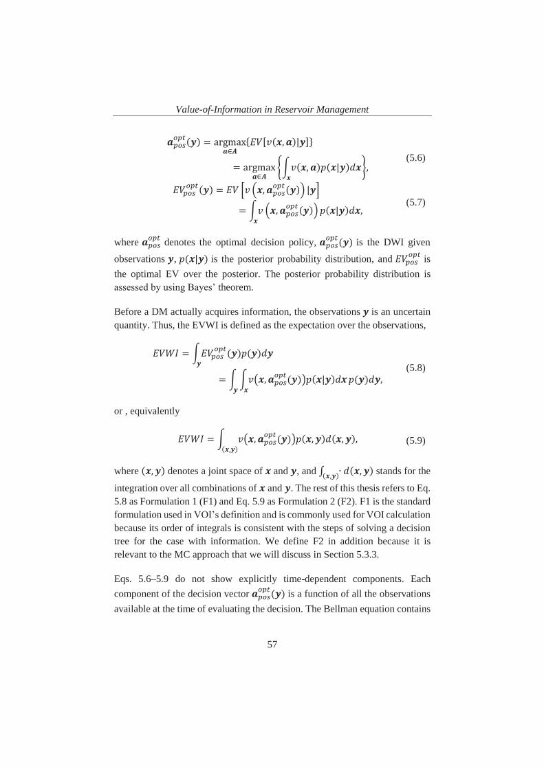
Value-of-Information in Reservoir Management
57
(5.6)
(5.7)
where denotes the optimal decision policy, is the DWI given
observations , is the posterior probability distribution, and is the optimal EV over the posterior. The posterior probability distribution is assessed by using Bayes’ theorem.
Before a DM actually acquires information, the observations is an uncertain quantity. Thus, the EVWI is defined as the expectation over the observations,
(5.8)
or , equivalently
(5.9)
where denotes a joint space of and , and stands for the
integration over all combinations of and . The rest of this thesis refers to Eq. 5.8 as Formulation 1 (F1) and Eq. 5.9 as Formulation 2 (F2). F1 is the standard formulation used in VOI’s definition and is commonly used for VOI calculation because its order of integrals is consistent with the steps of solving a decision tree for the case with information. We define F2 in addition because it is relevant to the MC approach that we will discuss in Section 5.3.3.
Eqs. 5.6–5.9 do not show explicitly time-dependent components. Each component of the decision vector is a function of all the observations available at the time of evaluating the decision. The Bellman equation contains

Value-of-Information in Reservoir Management
58
a complete expression of Eq. 5.8 for a time-dependent system (Eidsvik et al. 2015, Bellman 1957).
5.2 VOI Calculation for Continuous Probability Distributions
An analytical solution for Eq. 5.8 does not exist for many cases involving continuous probability distributions. In these contexts, VOI calculation can be performed only using numerical approximation. Such methods include MCS or discretization rules (e.g., extended Pearson-Tukey, McNamee-Celona shortcut, or extended Swanson-Megill). Bickel et al. (2011) compared these approximation methods for cases where both the prior and likelihood functions were normal distributions, and they concluded that all the above-mentioned discretization rules result in significant errors in the VOI estimate and that numerous MC samples are required for an accurate VOI estimate.
The accuracy of VOI estimate depends on the decision characteristics resulting from the probability distributions and how well these are preserved using a heuristic discretization method or MCS.
5.2.1 High Resolution Probability Tree Discretization Method
We introduce a discretization method called the high resolution probability tree (HRPT) approach, which approximates a probability distribution by discretizing the space of an uncertain quantity into numerous outcomes. The following briefly presents this approach and its advantage. More details on the development and discussion of the HRPT approach can be found in Paper IV.
Figure 5.1 illustrates the discretization of a probability distribution with 9 degrees18 and its comparison to MC sampling with 9 samples. The continuous probability distribution is represented by the blue curve, the HRPT discretized outcomes by the orange dots, and the MC samples by the black rings. The shape of the continuous probability distribution is better preserved by the HRPT 18 The number of degrees is referred to as the number of discrete outcomes, which is also the number of branches for an uncertainty node in a decision tree.

Value-of-Information in Reservoir Management
59
discretized outcomes than the MC samples because the HRPT discretized outcomes distribute evenly throughout the range of , whereas most of the MC samples cluster around the mode. Better preservation of the shape of the continuous probability distribution can better preserve the decisions characteristics and in turn improve the accuracy of VOI estimate.
If the number of degrees for HRPT equals the number of MC samples, the computational time for VOI estimation is the same using HRPT as using MCS. Thus, using HRPT won’t introduce additional computational time for VOI estimation, compared to MC method.
Figure 5.1—Illustration of HRPT discretized outcomes and MC samples for a continuous
probability distribution.
5.2.2 Accuracy of HRPT We investigate a two action linear-loss normal (TALL-N) problem to explore the accuracy of HRPT. The reason for using a TALL-N problem is that its VOI can be calculated analytically using the formula derived by Bickel (2008).
The TALL-N problem is as follows. A risk-neutral DM is considering whether or not to drill a well in an undeveloped area. The DM is uncertain about the NPV for the well and a priori characterizes it by a normal distribution with a mean of $10 million and an SD of $20 million. If the well is not drilled, the NPV is a sure $0. To improve this decision, a seismic survey can be conducted at a cost. The DM uses a positive correlation coefficient to describe the correlation between the true value of the well and the seismic results. We consider the value of being any of 0.70, 0.71, 0.72, …, 1.00 because the VOI

Value-of-Information in Reservoir Management
60
error is significant when for this example.19 The VOI for the seismic survey needs to be calculated to support the decision of whether the DM should pay for conducting the seismic survey. For this TALL-N problem, the VOI has a closed-form solution, as presented by Bickel (2008). In order to assess how well HRPT approximates the analytical solution for different values, we calculate the VOIs analytically and using HRPT with various degrees, and then calculate the error of the HRPT estimate relative to the analytical solution. The average relative VOI error is calculated by averaging over all the values. Figure 5.2 shows the average relative VOI error as a function of the number of degrees.
Figure 5.2—Average relative VOI error as a function of the number of degrees for the
TALL-N problem.
In this figure, the average relative VOI error decreases (i.e., the accuracy of HRPT increases) as the number of degrees increases. The average relative VOI error is as small as 3.5% with only 10 degrees, and it is further reduced to 0.25% with only 30 degrees.
Paper IV investigates the accuracy of applying HRPT for VOI estimation to two other structures of prior distribution—PERT and lognormal distributions. These distributions are used extensively in the O&G industry.
19 The value of is allowed to be any from 0 to 1.

Value-of-Information in Reservoir Management
61
5.2.3 Comparison of HRPT and MC-based Methods We compare the accuracy of using HRPT, Bayes Monte Carlo (BMC), and EnKF in estimating VOI for a TALL-N problem. Both of the latter two methods use MC sampling, but in different manners (see the appendices in Paper IV for detailed description of these two methods). This comparison provides an indication of how many MC samples are required to provide an equally good estimate as using HRPT.
The TALL-N problem for this comparison is as follows. A risk-neutral DM is considering whether to conduct a project: if the expected revenue of the project is positive, it will be conducted; otherwise, not conducted. The DM is uncertain about the revenue of the project and a priori characterizes it by a normal distribution with a mean of $3 million and an SD of $10 million. Information on the revenue can be obtained at a cost. The information has a Gaussian distributed error with zero mean and an SD of $5 million. The VOI for this information needs to be calculated to support the decision of whether the DM should pay for this information.
The comparison is shown in Figure 5.3. To achieve a relative VOI error of 0.75%, HRPT requires 20 degrees, EnKF requires 80 ensemble members, and BMC requires more than 18000 MC samples. To achieve a relative VOI error of 0.5%, the number of degrees for HRPT would need to be increased only to 30, but the necessary ensemble size for EnKF would exceed 10000 and the required number of MC samples for BMC would far exceed 18000.20 This indicates that HRPT is significantly more efficient than the other two methods in calculating the VOI for a TALL-N problem.
Although a closed-form solution exists for the TALL-N problem, this type of problem is constrained with Gaussian distributions, two actions, and linear value function. Thus, there is a need for more general solutions that would allow the VOI principle to be applied in real-world settings having any distributions,
20 We did not calculate the relative VOI errors from using EnKF with more than 10000 samples or the BMC with more than 18000 samples because our computer did not have sufficient memory.

Value-of-Information in Reservoir Management
62
any number of actions, and any value function. A possible solution will be illustrated and discussed in the next section.
Figure 5.3—Relative error of VOI estimates using HRDT, BMC, and EnKF.
5.3 VOI Calculation for Reservoir Management In a given RM context, there might be hundreds of relevant uncertain quantities. If we use HRPT with 30 degrees for each uncertain quantity, then having 100 uncertain quantities would mean 30100 combinations of discretized outcomes, once again raising the “curse of dimensionality.” Thus, a different method is required for calculating VOI for many RM decision problems.
5.3.1 Relationship between Terms in VOI Analysis and Reservoir Management
Decision analysts and reservoir engineers use different terms in VOI analysis. Thus, it can be difficult for decision analysts and reservoir engineers to understand each other and communicate efficiently on decision problems. To alleviate this difficulty, Table 5.1 gives the two disciplines’ corresponding terms for common VOI concepts.

Value-of-Information in Reservoir Management
63
Table 5.1—Relationship between terms used in VOI analysis and those in RM.

Value-of-Information in Reservoir Management
64
Assume a production model (e.g., an ECLIPSE reservoir simulation model) that formulates the dynamics of reservoirs is already given. Examples of the distinctions of interest in a RM context are the permeabilities in every grid block cell, and examples of the observable distinctions are the oil rates measured at different times. The priors are the probability distributions of the permeabilities based on current knowledge; the likelihoods are the probability distributions over the measured oil rates given the permeabilities; the preposteriors are the probability distributions over the measured oil rates; and the posteriors are the probability distributions over the permeabilities given the measured oil rates.
5.3.2 Decision-tree Example of VOI Calculation for Reservoir Management
We use a decision-tree example to illustrate the standard procedure of VOI analysis in an RM context.
We assume that a production model is given but that its parameters (say, the permeability distribution) are uncertain and that once we have determined the values for these parameters, the model itself will correctly “predict” future production. We consider three realizations of the permeability distribution, denoted , and . These realizations are equi-probable a priori. We are considering whether to measure and match the oil production rate at time . The information provided by the measured data is used to support the decision on choosing one of three production strategies , , and for time forward. We want to estimate the value of the data measurement at time .
The predicted oil production rates by the three realizations are shown in Figure 5.4, where is the oil production rate predicted for the period from time to , which is obtained by running the production model with parameters and a production strategy . If the measurement is perfect, we will definitely measure a high rate given the permeability distribution of
. Because of measurement errors, the probability of measuring a high rate is 4/5 and of measuring a low rate is 1/5 given . That is, the
likelihood and . The likelihood function is listed in Table 5.2.

Value-of-Information in Reservoir Management
65
Figure 5.4—Oil production rate profiles of three realizations.
Table 5.2—Likelihood function for the decision tree example.
Figure 5.5a shows the uncertainty tree with the prior and likelihood probabilities in assessed form. Its corresponding inferential form (flipped tree) is shown in Figure 5.5b, where the preposterior and posterior probabilities are shown. These probabilities are calculated using Bayes’ theorem, from the given prior and likelihood probabilities.
(a) Assessed Form: Information we have (b) Inferential Form: Information we need
Figure 5.5—Uncertainty trees in (a) assessed form, and (b) inferential form.
( )

Value-of-Information in Reservoir Management
66
The decision tree for the case with information, as illustrated in Figure 5.6 where all monetary values are in million USD, is constructed by including decision and payoff nodes in the flipped uncertainty tree (Figure 5.5b). Solving the decision tree yields the optimal decision policy that if we have measured a low rate , the optimal production strategy is ; if we have measured a high rate , the optimal production strategy is . This results in the optimal EV (i.e., EVWI) of $70.8 million.
Figure 5.6—Decision tree for the case with information.
Figure 5.7 illustrates the decision tree for the case without information. The DWOI is and EVWOI is $67.3 million. The VOI is thus $70.8 million – $67.3 million = $3.5 million. The information creates a value of $3.5 million because it holds the possibility to change the decision when it becomes available. If the cost of acquiring the information is lower than $3.5 million, we should conduct the measurement; otherwise, we should not.
Figure 5.7—Decision tree for the case without information.

Value-of-Information in Reservoir Management
67
5.3.3 VOI Calculation Using Ensemble-based Methods for Reservoir Management
MC sampling is an easily accessible and powerful approach to handle continuous probability distributions and numerous uncertain quantities. MC-based methods, such as EnKF for Bayesian inference and EnOpt for RO (i.e., identifying the optimal alternative), can also be used to calculate VOI, as will be discussed below.
5.3.3.1 The BvHJ Approach
An approach of using EnKF and EnOpt for VOI calculation was proposed by Barros et al. (2016). We refer to this as the BvHJ approach.
The BvHJ approach is derived using common terminology in reservoir engineering. It is based on a twin experiment where the DWI and DWOI are valued on a synthetic truth and where the difference between the values corresponding to the DWI and DWOI is calculated. A synthetic truth in the BvHJ approach is a realization drawn from the prior probability distribution.
realizations are first drawn from the prior probability distribution, one of which is then chosen as a synthetic truth, and the rest form the prior ensemble with realizations (Barros et al. 2016). The procedure of conducting a twin experiment is repeated for all synthetic truths. For each synthetic truth, there is a corresponding difference between its values corresponding to the DWI and DWOI. The BvHJ approach then calculates the VOI as the EV over all these differences associated with synthetic truths. Figure 5.8 shows the procedure of VOI calculation using the BvHJ approach.
In the BvHJ approach, the concept of synthetic truth is central to the analysis. However, “synthetic truth” has no meaning in VOI analysis. In reservoir engineering, a synthetically true model is used to mimic the actual state of a reservoir, by which reservoir engineers can investigate whether the actual outcome falls within the range that was predicted by updated models. This is not the case in VOI analysis, where the importance is to inform decisions, which in turn requires relevant and material uncertainties be quantified and analysis of how new information will update the distribution over the distinctions of interest and thus potentially affect the decisions. Moreover, VOI as defined by

Value-of-Information in Reservoir Management
68
Barros et al. (2016) implies a VOI distribution. However, as shown by Bratvold et al. (2009), the VOI is not a distribution but the difference between two expected values. Thus, the BvHJ approach is inconsistent with the definition of VOI analysis. However, two small modifications to the BvHJ approach can address this, as we will show later.
Figure 5.8—Procedure of VOI calculation using the BvHJ approach. Adapted from
Barros et al. (2016).
5.3.3.2 Derivation of an Approach Consistent with VOI’s Definition
Barros et al. (2016) did not elaborate on the connection between their approach and VOI analysis as defined in DA (Bratvold et al. 2009). We seek to accomplish this by deriving an approach using DA terminology and definitions.

Value-of-Information in Reservoir Management
69
Prior. MC samples are drawn from the prior probability distribution to form the prior ensemble [ , , …, ]. The probability of each sample
is . The prior ensemble is an MC representation of the prior probability distribution.
Likelihood. The likelihood function is assessed through a measurement noise distribution. For a dynamic system, we have the following mathematical relationship between the model parameters and measured data at time :
(5.10) (5.11)
where the subscript is the index of time, is a production model, and is a vector of the measurement noise at time . When using EnKF together with a reservoir simulation model, the standard practice is to assign a multivariate Gaussian distribution to with zero mean and a diagonal covariance matrix (i.e., ); this yields
. Therefore, assessing a probability distribution for the measurement noise is equivalent to assessing the likelihood function.
Preposterior. The MC samples representing the preposterior probability distribution can be generated as follows: (1) draw an MC sample from
(this is done when the prior ensemble has been generated), (2) run the model to time to obtain a realization of the predicted observations , (3) draw an MC sample from , (4) add to to obtain a sample of the observations with noise , and (5) repeat steps (1)–(3) to generate a set of , [ , , …, ], which is the preposterior ensemble representing the preposterior probability distribution. Moreover, the samples of ( , )-pairs [( , ), ( , ), …, ( , )] represent the joint probability distribution .
Posterior. The posterior ensemble [ , , …, ], representing the posterior probability distribution , is generated by using EnKF to update the prior ensemble with the given observations and assessed measurement noise .

Value-of-Information in Reservoir Management
70
DWOI and EVWOI. We identity the DWOI and calculate the EVWOI using Eq. 5.12 (the MC form of Eq. 5.4) and Eq. 5.13 (the MC form of Eq. 5.5), respectively,
(5.12)
(5.13)
DWI. We identify the DWI for the given observations using Eq. 5.14 (the MC form of Eq. 5.6),
(5.14)
EVWI. The EVWI can be calculated using either Eq. 5.15 (the MC form of F1 (Eq. 5.8)),
(5.15)
or Eq. 5.16 (the MC form of F2 (Eq. 5.9)),
(5.16)
VOI. The VOI is calculated using Eqs. 5.2 and 5.3.
A schematic of VOI calculation using MC-based methods is shown in Figure 5.9.

Value-of-Information in Reservoir Management
71
Figure 5.9—Schematic of VOI calculation using MC-based methods.
5.3.3.3 Comparison of the Approaches for VOI Calculation
The F2 approach is compared first with the BvHJ approach and then with the F1 approach.
F2 Approach vs. BvHJ Approach. There are two differences between these approaches. The first is that in the F2 approach, no realization is excluded from the prior ensemble; whereas in the BvHJ appraoch, a “synthetic truth” is excluded from the prior ensemble and the remaining ensemble members form a new prior ensemble. This difference leads to different VOI estimates as will be discussed later. The second difference is that the F2 approach calculates VOI as the difference between two EVs, whereas the BvHJ approach calculates VOI as an EV of a set of differences. Although the second difference does not affect

Value-of-Information in Reservoir Management
72
the VOI estimate, it constitutes a conceptual difference. The BvHJ approach with two minor modifications with respect to these two differences is identical to the F2 approach that is consistent with the VOI definition.
F2 Approach vs. F1 Approach. Based on the law of large numbers, these two approaches give the same limit when the ensemble size approaches infinity. However, the convergence rate can be different, resulting in different estimates when the ensemble size is small because these two approaches introduce different levels of sampling error.
Accuracies of the Approaches. We use an example to investigate the accuracy of the VOI estimates of the three approaches.
Consider that the distinction of interest is the revenue of a project and that the observable distinction is the information on the revenue. The relationship of
, , and the error of the information is . A priori, is normally distributed with mean and standard deviation , i.e., the prior
. is normally distributed with zero mean and standard deviation , i.e., the likelihood function . The decision to be made is whether the project will be conducted; and correspond to “conduct” and “not conduct,” respectively. If the expected revenue is positive, the project should be conducted; otherwise, it should not. Thus, the value function is . With , and (the monetary unit can be arbitrary here), the VOI for this problem setting can be calculated analytically, which is 2267.
We first test the three approaches using a large ensemble size: 10000. The VOI estimates are listed in Table 5.3. The BvHJ approach gives a result almost identical to that of the F2 approach because the impact of excluding a “synthetic truth” (i.e., an ) from the prior ensemble is very small when the ensemble size is large. The VOIs calculated using the F1 and F2 approaches differ slightly. All three methods estimate the VOI with an error smaller than 1%.

Value-of-Information in Reservoir Management
73
Approach Analytical BvHJ F1 F2 VOI 2267 2283 2246 2283
Error - 0.71% 0.93% 0.71% Table 5.3—VOI estimates using BvHJ, F1, and F2 approaches with ensemble size of
10000.
Then, a small ensemble size, 50, is used. The VOI calculation is repeated 10000 times for each approach. The statistics of the VOI estimates are listed in Table 5.4, and the probability density functions (PDFs) are plotted in Figure 5.10.21 Among the three approaches, the F2 approach is the most accurate, as it gives the best VOI estimate on average and has the smallest SD in its estimates. More detail on why the F2 approach is better is given in Paper V.
Approach BvHJ F1 F2 Average 2323 2257 2259
Error 2.47% 0.44% 0.35% SD 933 776 695
[Min, Max] [0, 10421] [0, 5497] [0, 5279] Table 5.4—Statistics of VOI estimates of BvHJ, F1, and F2 approaches with ensemble size
of 50.
Figure 5.10—PDFs of VOI estimates of BvHJ, F1, and F2 approaches with ensemble size
of 50.
This example has demonstrated that the three approaches give almost equivalent results for large ensembles. However, they can lead to quite different results when the ensemble size is small. As there are no significant
21 Here, the uncertainty in the VOI estimate is due to the sampling error associated with MC methods. As discussed earlier, the VOI itself is not a distribution but the difference between two expected values.

Value-of-Information in Reservoir Management
74
computational increases resulting from using the F2 approach for VOI calculation with MC methods, this would be our approach of choice.
5.3.3.4 Example of Applying the F2 Approach with a Reservoir Simulation Model
We briefly show an example of applying the F2 approach to estimate VOI for a more realistic case, where a reservoir simulation model is involved. For more details on the model and problem setting, please refer to Paper V.
VOI analysis is used to analyze whether devices should be placed for acquiring saturation data, in addition to oil and water production rate data. The measured data are used to support the decision on polymer concentration in the enhanced-oil-recovery (EOR) phase.
The VOI is calculated using the F2 approach combined with EnKF and EnOpt. The resulting VOIs for rate data only, saturation data only, and both rate and saturation data, and VOPI are listed in Table 5.5. The values of rate data and saturation data are very close to each other. Although the saturation data has a value of $3.36∙105 when it is considered individually, it adds a value of only $1.01∙105 (= $4.11∙105 – $3.10∙105) to that of the rate data. This indicates that VOI is not additive (Samson et al. 1989). The VOI analysis informs us that we should not gather saturation data in addition to rate data if the cost of placing saturation measuring devices is greater than $1.01∙105. The VOPI is $6.12∙105, which is $6.12∙105 – $3.10∙105 = $3.02∙105 more than the value of rate data. Therefore, we should decline any other data gathering activity that costs more than $3.02∙105 given that the rate data will be gathered.
Data Type Rate Only
Saturation Only
Rate and Saturation
Perfect Information
VOI [105 USD] 3.10 3.36 4.11 6.12 Table 5.5—VOI estimates for the example with a reservoir simulation model.

Overview of Research Papers
75
6 Overview of Research Papers
Paper I: Integrating Model Uncertainty in Probabilistic Decline Curve Analysis for Unconventional Oil Production Forecasting
This paper introduces an approach to integrating model uncertainty in probabilistic decline curve analysis. The aim is to assess the probabilities of different decline curve models and use these probabilities for further analysis instead of identifying and using a “best” model for decline curve analysis. We focus on unconventional oil production because the widely used Arps decline curve model might not be ideal for unconventional play; thus, several novel decline curve models have been proposed. Examples are used to illustrate the impact of the integration of model uncertainty. The proposed approach is applied to real data. We conclude that using our proposed approach can reduce the risk of using a best fit but very wrong model for forecasting and that our proposed approach performs well in propagating the model uncertainty to the uncertainty in forecast.
Paper II: Robust Production Optimization with Capacitance-Resistance Model as Precursor
This paper presents a proxy-model workflow where a grid-based model is supplemented by a useful yet tractable proxy model for speeding up the process of RO. Specifically, we review CRMs as potential proxy models for waterflooding systems. A selected CRM is embedded into the proxy-model workflow. We illustrate the use of a CRM and investigate its pros and cons using synthetic 2D and 3D models. The results obtained from the proxy-model and traditional workflows are compared. The impact of any differences is assessed, and the value of using a proxy model is quantified by considering a PO-relevant decision-making context. We discuss the desiderata of proxy models. We conclude that CRMs have high potential to serve as a cogent proxy model for waterflooding-related decision-making contexts and that the proxy-model workflow, leveraging a faster but relevant production model, significantly speeds up the optimization yet gives robust results that lead to a near-optimal solution.

Overview of Research Papers
76
Paper III: Fast Analysis of Optimal IOR Start Time Using a Two-Factor Production Model and Least-Squares Monte Carlo Algorithm
This paper presents an approach of using a two-factor production model together with the LSM algorithm for fast analysis of optimal IOR start time. We review the two-factor production model introduced by Parra-Sanchez (2010). This production model is computationally more attractive than a more complex model, such as a reservoir simulation model. Thus, using it can significantly speed up the uncertainty analysis where a large number of production forecast runs is required. Identifying the optimal IOR start time using LSM allows for learning over time. Unlike the myopic decision policy, which considers only the current information, LSM considers both the current information and the information that will be obtained in the future. Therefore, the LSM solves approximately for the global optimum of an FSRM problem. The impact of allowing learning over time in decision making is quantified using the VOI framework. An example illustrates the application of the proposed approach. We conclude that combining the two-factor model with LSM facilitates a fast analysis of optimal IOR start time and that it can create significant value to include learning over time in decision making.
Paper IV: Robust Discretization of Continuous Probability Distributions for Value-of-Information Analysis
This paper introduces a practical, flexible, efficient, and very general discretization method for continuous probability distributions involved in VOI analysis. This discretization method is validated by comparing its VOI estimate to the analytical solutions. Commonly used discretization methods for VOI calculation are reviewed and compared to the proposed method. In addition, we investigate two MC-based methods for VOI calculation. We conclude that the proposed discretization method estimates VOI very accurately (with a relative error of around 0.25% using a degree of discretization of only 30), that the commonly used discretization methods generally give poor VOI estimates, and that more than thousands of MC samples are required for the MC-based methods to provide accurate VOI estimates.

Overview of Research Papers
77
Paper V: Value-of-Information for Model Parameter Updating through History Matching
This paper presents a consistent, DA-based VOI analysis framework to assess the value of HM. It is consistent and DA-based because it is derived from VOI’s definition originally developed in the DA community. In order to make the VOI framework understandable and accessible to both the RM and DA communities, we bridge the nomenclature and terminology used in VOI calculations and that used in state-of-the-art HM and PO methods. In particular, our framework uses EnKF for Bayesian inference and EnOpt for RO. We discuss two formulations (F1 and F2) of VOI calculation. In addition, we investigate the similarities and differences between the F2 approach and the BvHJ approach. Several examples are used to illustrate and discuss the use of this framework in an HM context. We conclude that the BvHJ approach with two minor modifications will be identical to the F2 approach, and that the F2 approach gives the most accurate VOI estimate among the three approaches investigated.

Summary and Conclusions
78
7 Summary and Conclusions
RM involves a process of gathering data and information to inform and support decision making. HM is used to extract information from measured data. The information is then used to support the decisions on production strategies through an optimization process. Thus, RM is a decision-oriented activity, for which a DA framework will add value.
The major goal of DA is to make good decisions. This requires the quantification of relevant and material uncertainties, a consistent way of updating uncertainties when new information arrives, and a means to assess the value of such information. We referred to this combination of activities as “decision-focused uncertainty management.” 22 This work illustrated and discussed a decision-focused uncertainty-management framework for RM using DA tools, with a focus on geological uncertainty.
We first investigated how geological uncertainty should be managed for the goal of making good decisions in HM and PO separately, and then investigated how it should be managed in RM as a loop of HM and PO. We finally investigated how to incorporate a powerful decision analysis tool—VOI analysis—into RM.
To manage geological uncertainty in HM, HM should be conducted probabilistically rather than deterministically. Probabilistic HM approaches use probability distributions to quantify uncertainties. Probabilistic HM can be achieved by simply repeating deterministic HM in an MC manner, such as the Bootstrap method (Section 2.1.2.2) or the P-MLE method (Section 2.1.2.3). When normal distributions are used to represent a DM’s uncertainties, EnKF is a proven method for Bayesian HM. It can efficiently update a production model with numerous uncertain parameters. To integrate model uncertainty in decline curve analysis, we proposed an approach to assess the probabilities of various decline curve models by repeating the P-MLE method for each decline curve
22 For brevity, the phrase “decision-focused uncertainty management” was simply referred to as “uncertainty management” throughout this thesis.

Summary and Conclusions
79
model, and concluded that considering model uncertainty gives a more complete estimate of uncertainty in a production forecast.
Geological uncertainty in PO can be managed by optimizing the EV over geological realizations if the DM is risk-neutral. This is known as RO. However, the challenge is that when a traditional optimization algorithm is used, to optimize the EV over numerous geological realizations is much more computationally intensive than to optimize the value of a single realization. EnOpt is designed to address this challenge. It is based on the traditional steepest ascent method, but it uses a more efficient approach to approximate the gradient. Although EnOpt has significantly sped up RO, the computational time can still be long when a reservoir simulation model is involved. Thus, we proposed a proxy-model workflow where a CRM is used to supplement a reservoir simulation model for RO. The results showed that the proxy-model workflow gives a near-optimal solution with significantly reduced computational time.
CLRM is a state-of-the-art approach to managing geological uncertainty in RM. It closes the loop of HM and PO by continuously updating a production model and performing life-cycle optimization whenever new data become available. However, it is based on a myopic decision policy, in that it does not account for future uncertainty revelations and their impacts on future decisions. Thus, the CLRM solution can be suboptimal. Since RM is a sequential decision-making problem, it should consider whether geological uncertainty informed by current data or by future information. We demonstrated the full structure of a dynamic programming approach to RM decision making using decision trees. FSRM has a more complex structure and requires longer computational time than does CLRM. However, the optimal solution of FSRM is a global optimum. The LSM algorithm is very efficient for solving an FSRM problem with relatively small numbers of decisions and of decision alternatives. It does not suffer from the “curse of dimensionality” as the number of uncertainties increases. We illustrated this by an example of using LSM combined with a two-factor model to identify the optimal IOR start time.
VOI analysis assesses the value of additional information before it is obtained. The assessed value is used to support the decision on whether to buy the additional information. We proposed the HRPT method to discretize

Summary and Conclusions
80
continuous probability distributions used in VOI calculation. It was compared with other common discretization methods and MC-based methods. The comparison showed that HRPT provides significantly more accurate VOI estimates than do the other methods.
Although the concept of VOI has been illustrated and discussed in an RM context by other research, there is a gap between the terms used in the DA and RM communities for VOI analysis. This may make the communication between these two communities difficult. To reduce the gap, we related the RM terminology to the VOI terminology commonly used in DA and derived a general VOI analysis framework for RM, based on VOI’s definition. We compared the VOIs estimated using different formulations. We found that although these formulations give the same analytical results, the results from their numerical implementations can be different when MC methods are used. The results showed that the F2 approach provides a more accurate VOI calculation.
This thesis used several examples to illustrate insights and guidance for managing geological uncertainty with DA tools in RM. Challenges remain in practice that might prevent the development of a broad and deep understanding and routine application of DA. Nevertheless, we are optimistic about the value of applying DA in RM and the entire O&G industry.

Discussion and Future Research
81
8 Discussion and Future Research
Our work has shown the value of implementing DA to manage geological uncertainty in RM. We propose the following areas for future research.
As engineers and geoscientists, we have been taught a modeling philosophy that emphasizes detailed deterministic realism. However, as the main purpose of a model used in an RM context is to inform and support decisions, we need to evaluate whether any model is useful and tractable for that purpose. Building in a lot of details into our production models (e.g., building reservoir simulation models) might not serve this purpose. Less detailed models that allow us to consistently capture our uncertainties will often do a better job in informing and supporting decision making. Details can then be added to the model if they are deemed to be relevant and material for the decisions at hand.
Although the current state-of-the-art production models are suitable for some types of RM decision, they often include detailed features that are not relevant and material for other decisions. This makes decision analysis for RM computationally intensive or even prohibitive. More focus should be on production models that are both useful and tractable for decision making. CRM is a cogent model for the context of deciding water injection rates for waterflooding. It should be extended to include more features (e.g., adding new wells and chemical flooding) so that other RM-relevant decision contexts can benefit from its speed.
CLRM, as the state-of-the-art RM tool, is based on a myopic decision policy and thus can result in suboptimal solutions. Because the computational requirement for solving a CLRM problem is significantly less than that for an FSRM problem, CLRM might be regarded as a simplification of FSRM. However, it is never a substitute for FSRM. Future research should focus on investigating the differences between CLRM and FSRM solutions and on more efficient methods for solving an FSRM problem.
Since data are gathered for informing decisions on production strategies, HM should be decision-driven rather than data-driven. “Data-driven” means that we first gather data and then consider what decision the data can inform. In contrast, “decision-driven” means we first identify the decisions we are going

Discussion and Future Research
82
to make and then consider what data should be gathered to inform these decisions. The advantage of decision-driven HM is that we can avoid spending money on valueless data gathering activities. Thus, future research should focus on decision-driven HM using a VOI analysis framework.
Our work considers only one decision point in VOI analysis for RM. Although Barros et al. (2015) extended the BvHJ approach to account for sequential decisions, they calculate the exclusive VOI for CLRM rather than the general VOI for FSRM. Because CLRM might result in suboptimal solutions as discussed earlier, the VOI for CLRM may be smaller than the VOI for FSRM (the VOI defined in the DA community). Focus should be on efficient methods to calculate the VOI for FSRM.
The present work focused on geological uncertainty. Future research should also consider economic uncertainty (e.g., the uncertainty in oil price) in RM.

References
83
References
Aanonsen, S.I., Nævdal, G., Oliver, D.S. et al. 2009. The Ensemble Kalman Filter in Reservoir Engineering—a Review. SPE Journal 14 (3): 393-412. SPE-117274-PA. https://doi.org/10.2118/117274-PA.
Arps, J.J. 1945. Analysis of Decline Curves. Transactions of the AIME 160 (1): 228-247. SPE-945228-G. https://doi.org/10.2118/945228-G.
Barker, J.W., Cuypers, M., Holden, L. 2000. Quantifying Uncertainty in Production Forecasts: Another Look at the PUNQ-S3 Problem. Presented at the SPE Annual Technical Conference and Exhibition, Dallas, USA, 1-4 October. SPE-62925-MS. https://doi.org/10.2118/62925-MS.
Barros, E., Leeuwenburgh, O., Van den Hof, P. et al. 2015. Value of Multiple Production Measurements and Water Front Tracking in Closed-Loop Reservoir Management. Presented at the SPE Reservoir Characterisation and Simulation Conference and Exhibition, Abu Dhabi, UAE, 14-16 September. SPE-175608-MS. https://doi.org/10.2118/175608-MS.
Barros, E., Van den Hof, P., Jansen, J. 2016. Value of Information in Closed-Loop Reservoir Management. Computational Geosciences 20 (3): 737-749. https://doi.org/10.1007/s10596-015-9509-4.
Begg, S.H., Welsh, M.B., Bratvold, R.B. 2014. Uncertainty vs. Variability: What's the Difference and Why is it Important? Presented at the SPE Hydrocarbon Economics and Evaluation Symposium, Houston, USA, 19-20 May. SPE-169850-MS. https://doi.org/10.2118/169850-MS.
Bellman, R.E. 1957. Dynamic Programming. New Jersey, USA: Princeton University Press.
Bickel, J.E. 2008. The Relationship Between Perfect and Imperfect Information in a Two-Action Risk-Sensitive Problem. Decision Analysis 5 (3): 116-128.
Bickel, J.E., Bratvold, R.B. 2008. From Uncertainty Quantification to Decision Making in the Oil and Gas Industry. Energy Exploration & Exploitation 26 (5): 311-325. https://doi.org/10.1260/014459808787945344.
Bickel, J.E., Lake, L.W., Lehman, J. 2011. Discretization, Simulation, and Swanson's (Inaccurate) Mean. SPE Economics & Management 3 (3): 2150-1173. SPE-148542-PA. https://doi.org/10.2118/148542-PA.
Box, G.E. 1979. Robustness in the Strategy of Scientific Model Building. In Robustness in Statistics, 201-236. New York, USA: Academic Press.

References
84
Bratvold, R.B., Begg, S. 2009. Would You Know a Good Decision if You Saw One? The Way Ahead 5 (2): 21-23. SPE-0209-021-TWA. https://doi.org/10.2118/0209-021-TWA.
Bratvold, R.B., Begg, S. 2010. Making Good Decisions. Texas, USA: Society of Petroleum Engineers.
Bratvold, R.B., Bickel, J.E., Lohne, H.P. 2009. Value of Information in the Oil and Gas Industry: Past, Present, and Future. SPE Reservoir Evaluation & Engineering 12 (4): 630-638. SPE-110378-PA. https://doi.org/10.2118/110378-PA.
Brouwer, D.R., Nævdal, G., Jansen, J.D. et al. 2004. Improved Reservoir Management Through Optimal Control and Continuous Model Updating. Presented at the SPE Annual Technical Conference and Exhibition, Houston, Texas, 26-29 September. SPE-90149-MS. https://doi.org/10.2118/90149-MS.
Burgers, G., Jan van Leeuwen, P., Evensen, G. 1998. Analysis Scheme in the Ensemble Kalman Filter. Monthly Weather Review 126 (6): 1719-1724. https://doi.org/10.1175/1520-0493(1998)126<1719:ASITEK>2.0.CO;2.
Cao, F. 2014. Development of a Two-Phase Flow Coupled Capacitance Resistance Model. PhD Thesis, University of Texas at Austin, Austin, USA.
Cao, F., Luo, H., Lake, L.W. 2015. Oil-Rate Forecast by Inferring Fractional-Flow Models From Field Data With Koval Method Combined With the Capacitance-Resistance Model. SPE Reservoir Evaluation & Engineering 18 (4): 534-553. SPE-173315-PA. https://doi.org/10.2118/173315-PA.
Chen, Y., Oliver, D.S., Zhang, D. 2009. Efficient Ensemble-Based Closed-Loop Production Optimization. SPE Journal 14 (4): 634-645. SPE-112873-PA. https://doi.org/10.2118/112873-PA.
Cheng, Y., Wang, Y., McVay, D. et al. 2010. Practical Application of a Probabilistic Approach to Estimate Reserves Using Production Decline Data. SPE Economics & Management 2 (1): 19-31. SPE-95974-PA. https://doi.org/10.2118/95974-PA.
Clark, A.J., Lake, L.W., Patzek, T.W. 2011. Production Forecasting with Logistic Growth Models. Presented at the SPE Annual Technical Conference and Exhibition, Denver, USA, 30 October-2 November. SPE-144790-MS. https://doi.org/10.2118/144790-MS.
Clarkson, C.R., McGovern, J.M. 2005. Optimization of CBM Reservoir Exploration and Development Strategies through Integration of Simulation and Economics. SPE Reservoir Evaluation & Engineering 8 (6): 502-519. SPE-88843-PA. https://doi.org/10.2118/88843-PA.

References
85
Do, S.T., Reynolds, A.C. 2013. Theoretical Connections between Optimization Algorithms based on an Approximate Gradient. Computational Geosciences 17 (6): 959-973. https://doi.org/10.1007/s10596-013-9368-9.
Duong, A.N. 2011. Rate-Decline Analysis for Fracture-Dominated Shale Reservoirs. SPE Reservoir Evaluation & Engineering 14 (3): 377-387. SPE-137748-PA. https://doi.org/10.2118/137748-PA.
ECLIPSE. 2016. http://www.software.slb.com/products/eclipse (accessed 12 October 2016).
Eidsvik, J., Mukerji, T., Bhattacharjya, D. 2015. Value of Information in the Earth Sciences: Integrating Spatial Modeling and Decision Analysis. Cambridge, UK: Cambridge University Press.
Eppel, T., von Winterfeldt, D. 2008. Value-of-Information Analysis for Nuclear Waste Storage Tanks. Decision Analysis 5 (3): 157-167.
Evensen, G. 1994. Sequential Data Assimilation with a Nonlinear Quasi-Geostrophic Model Using Monte Carlo Methods to Forecast Error Statistics. Journal of Geophysical Research: Oceans 99 (C5): 10143-10162. https://doi.org/10.1029/94JC00572.
Evensen, G. 2009. Data Assimilation: The Ensemble Kalman Filter. Berlin, Germany: Springer Science & Business Media.
Floris, F.J.T., Bush, M.D., Cuypers, M. et al. 2001. Methods for Quantifying the Uncertainty of Production Forecasts: a Comparative Study. Petroleum Geoscience 7: S87-S96. https://doi.org/10.1144/petgeo.7.S.S87.
Fonseca, R.M., Stordal, A.S., Leeuwenburgh, O. et al. 2014. Robust Ensemble-based Multi-Objective Optimization. Presented at the ECMOR XIV-14th European Conference on the Mathematics of Oil Recovery Catania, Italy, 8-11 September. https://doi.org/10.3997/2214-4609.20141895
Gentil, P.H. 2005. The Use of Multilinear Regression Models in Patterned Waterfloods: Physical Meaning of the Regression Coefficients. Master's Thesis, University of Texas at Austin, Austin, USA.
Grayson, C.J. 1960. Decisions under Uncertainty: Drilling Decisions by Oil and Gas Operators. Cambridge, USA: Graduate School of Business, Harvard University.
Hajizadeh, Y., Christie, M.A., Demyanov, V. 2010. Comparative Study of Novel Population-based optimization Algorithms for History Matching and Uncertainty Quantification: PUNQ-S3 Revisited. Presented at the Abu Dhabi International Petroleum Exhibition and Conference, Abu Dhabi, UAE, 1-4 November. SPE-136861-MS. https://doi.org/10.2118/136861-MS.

References
86
Haldorsen, H.H., Van Golf-Racht, T. 1989. Reservoir Management into the Next Century. Presented at the New Mexico Tech Centennial Symposium, Socorro, USA, 16-19 October.
Hastie, T., Tibshirani, R., Friedman, J. 2009. The Elements of Statistical Learning : Data Mining, Inference, and Prediction. New York, USA: Springer.
He, J., Sarma, P., Bhark, E. et al. 2017. Quantifying Value of Information Using Ensemble Variance Analysis. Presented at the SPE Reservoir Simulation Conference, Montgomery, USA, 20-22 February. SPE-182609-MS. https://doi.org/10.2118/182609-MS.
Howard, R.A. 1966. Information Value Theory. IEEE Transactions on Systems Science and Cybernetics 2 (1): 22-26. https://doi.org/10.1109/TSSC.1966.300074.
Ilk, D., Rushing, J.A., Perego, A.D. et al. 2008. Exponential vs. Hyperbolic Decline in Tight Gas Sands: Understanding the Origin and Implications for Reserve Estimates Using Arps' Decline Curves. Presented at the SPE Annual Technical Conference and Exhibition, Denver, USA, 21-24 September. SPE-116731-MS. https://doi.org/10.2118/116731-MS.
Jannink, J.W., Bos, C.F.M. 2005. Probabilistic Discharge Forecasting for Improved Asset Investment Decision Support (SPE94116). Presented at the 67th EAGE Conference & Exhibition, Madrid, Spain, 13-16 June.
Jansen, J.-D., Brouwer, R., Douma, S.G. 2009. Closed Loop Reservoir Management. Presented at the SPE Reservoir Simulation Symposium, The Woodlands, Texas, 2-4 February. SPE-119098-MS. https://doi.org/10.2118/119098-MS.
Jochen, V.A., Spivey, J.P. 1996. Probabilistic Reserves Estimation Using Decline Curve Analysis with the Bootstrap Method. Presented at the SPE Annual Technical Conference and Exhibition, Denver, USA, 6-9 October. SPE-36633-MS. https://doi.org/10.2118/36633-MS.
Jonkman, R.M., Bos, C.F.M., Morgan, D.T.K. et al. 2010. Best Practices and Methods in Hydrocarbon Resource Estimation, Production and Emissions Forecasting, Uncertainty Evaluation, and Decision Making. SPE Reservoir Evaluation & Engineering 5 (2): 146-153. SPE-77280-PA. https://doi.org/10.2118/77280-PA.
Joshi, K., Lee, W.J. 2013. Comparison of Various Deterministic Forecasting Techniques in Shale Gas Reservoirs. Presented at the SPE Hydraulic Fracturing Technology Conference, The Woodlands, USA, 4-6 February. SPE-163870-MS. https://doi.org/10.2118/163870-MS.

References
87
Kalman, R.E. 1960. A New Approach to Linear Filtering and Prediction Problems. Journal of Basic Engineering 82 (1): 35-45. https://doi.org/10.1115/1.3662552.
Koval, E.J. 1963. A Method for Predicting the Performance of Unstable Miscible Displacement in Heterogeneous Media. Society of Petroleum Engineers Journal 3 (2): 145-154. SPE-450-PA. https://doi.org/10.2118/450-PA.
Kullawan, K. 2016. A Bayesian Framework for Real-Time Optimization of Well Placement. PhD Thesis, University of Stavanger, Stavanger, Norway.
Longstaff, F.A., Schwartz, E.S. 2001. Valuing American Options by Simulation: A Simple Least-Squares Approach. The Review of Financial Studies 14 (1): 113-147. https://doi.org/10.1093/rfs/14.1.113.
Lorentzen, R.J., Fjelde, K.K., Frøyen, J. et al. 2001. Underbalanced and Low-head Drilling Operations: Real Time Interpretation of Measured Data and Operational Support. Presented at the SPE Annual Technical Conference and Exhibition, New Orleans, USA, 30 September-3 October. SPE-71384-MS. https://doi.org/10.2118/71384-MS.
MATLAB. 2016. http://se.mathworks.com/products/matlab (accessed 12 October 2016).
Morgan, M.D. 2005. A Model of Canadian Oil and Gas Price Fluctuations. Journal of Canadian Petroleum Technology 44 (7). PETSOC-05-07-03. https://doi.org/10.2118/05-07-03.
Nævdal, G., Brouwer, D.R., Jansen, J.-D. 2006. Waterflooding Using Closed-Loop Control. Computational Geosciences 10 (1): 37-60. https://doi.org/10.1007/s10596-005-9010-6.
Pan, Z. 2016. Revised Productivity Index Equation to Improve Transient History Match for the Capacitance Resistance Model. Master's Thesis, University of Texas at Austin, Austin, USA.
Parra-Sanchez, C. 2010. A Life Cycle Optimization Approach to Hydrocarbon Recovery. Master Thesis, University of Texas at Austin, Austin, USA.
Raiffa, H., Schlaifer, R. 1961. Applied Statistical Decision Theory. New York, USA: Wiley.
Robertson, J.D. 1989. Reservoir Management Using 3D Seismic Data. Journal of Petroleum Technology 41 (7): 663-667. SPE-19887-PA. https://doi.org/10.2118/19887-PA.
Satter, A., Varnon, J.E., Hoang, M.T. 1994. Integrated Reservoir Management. Journal of Petroleum Technology 46 (12): 1057-1064. SPE-22350-PA. https://doi.org/10.2118/22350-PA.
References
88
Sayarpour, M. 2008. Development and Application of Capacitance-Resistive Models to Water/CO2 Floods. PhD Thesis, University of Texas at Austin, Austin, USA.
Sayarpour, M., Kabir, C., Sepehrnoori, K. et al. 2011. Probabilistic History Matching with the Capacitance–Resistance Model in Waterfloods: a Precursor to Numerical Modeling. Journal of Petroleum Science and Engineering 78 (1): 96-108. https://doi.org/10.1016/j.petrol.2011.05.005.
Sayarpour, M., Zuluaga, E., Kabir, C.S. et al. 2009. The Use of Capacitance–Resistance Models for Rapid Estimation of Waterflood Performance and Optimization. Journal of Petroleum Science and Engineering 69 (3): 227-238. https://doi.org/10.1016/j.petrol.2009.09.006.
Schlaifer, R. 1959. Probability and Statistics for Business Decisions. New York, USA: McGraw-Hill.
Skov, A.M. 1995. An Analysis of Forecasts of Energy Supply, Demand, and Oil Prices. Presented at the SPE Hydrocarbon Economics and Evaluation Symposium, Dallas, USA, 26-28 March. SPE-30058-MS. https://doi.org/10.2118/30058-MS.
Tavassoli, Z., Carter, J.N., King, P.R. 2004. Errors in History Matching. SPE Journal 9 (3): 352-361. SPE-86883-PA. https://doi.org/10.2118/86883-PA.
Thomas, P. 2016. Managing Uncertainty with Decision Analysis in The Oil and Gas Industry. PhD Thesis, University of Stavanger, Stavanger, Norway.
Thomas, P., Bratvold, R.B. 2015. A Real Options Approach to the Gas Blowdown Decision. Presented at the SPE Annual Technical Conference and Exhibition, Houston, Texas, 28-30 September. SPE-174868-MS. https://doi.org/10.2118/174868-MS.
Valko, P.P., Lee, W.J. 2010. A Better Way to Forecast Production from Unconventional Gas Wells. Presented at the SPE Annual Technical Conference and Exhibition, Florence, Italy, 19-22 September. SPE-134231-MS. https://doi.org/10.2118/134231-MS.
Wang, C., Li, G., Reynolds, A.C. 2009. Production Optimization in Closed-Loop Reservoir Management. SPE Journal 14 (3): 506-523. SPE-109805-PA. https://doi.org/10.2118/109805-PA.
Wiggins, M., Startzman, R. 1990. An Approach to Reservoir Management Presented at the SPE Annual Technical Conference and Exhibition, New Orleans, USA, 23-26 September. SPE-20747-MS. https://doi.org/10.2118/20747-MS.

References
89
Willis, H.H., Moore, M. 2013. Improving the Value of Analysis for Biosurveillance. Decision Analysis 11 (1): 63-81. https://doi.org/10.1287/deca.2013.0283.
Wolff, M. 2010. Probabilistic Subsurface Forecasting-What Do We Really Know? Journal of Petroleum Technology 62 (5): 86-92. SPE-118550-JPT. https://doi.org/10.2118/118550-JPT.
Wright, S.J., Nocedal, J. 1999. Numerical optimization. Berlin, Germany: Springer.


Paper I
Integrating Model Uncertainty in Probabilistic Decline Curve Analysis for
Unconventional Oil Production Forecasting
Hong, A.J., Bratvold, R.B., and Lake, L.W.


Integrating Model Uncertainty in Probabilistic Decline Curve Analysis for Unconventional Oil Production Forecasting 1
Manuscript Integrating Model Uncertainty in Probabilistic Decline Curve Analysis for Unconventional Oil Production Forecasting Aojie Hong and Reidar B. Bratvold, University of Stavanger and The National IOR Centre of Norway; and Larry W. Lake, University of Texas at Austin
Abstract Decline curve analysis is an industry-accepted and extensively used method in the oil and gas industry. As a result of the realization that the long-used Arps model may not be ideal for describing flow from unconventional plays, and may lack physical parameters, several models have been developed to capture the characteristics of different flow regimes.
model has a unique extrapolation and uncertainty. No one model is best in all circumstances, so instead of identifying a single production, we propose to regard any model as a potentially good model whose goodness is described by a probability representation. These probabilities of the models are further used to weight the model forecasts.
The main contributions of this work are (1) using probability to describe the goodness of a model, (2) an approach to integrate the model uncertainty in probabilistic decline curve analysis, (3) illustration and discussion of the impact of the model uncertainty, and (4) to illustrate our proposed approach in a real case.
We demonstrate and conclude that using our proposed approach can reduce the risk of using a best fit but very wrong model for forecasting. Our proposed approach performs well in propagating the model uncertainty to the uncertainty in forecast. Introduction Although numerical techniques for forecasting hydrocarbon production have developed rapidly over the past decades, decline curve analysis (DCA) remains an industry-accepted method that is used extensively in the oil and gas industry. Decline curve models are very computational attractive because only production data, which can be easily acquired, is required for determining the parameter values of a decline curve model through history matching. The history-matched model is further used for forecasting the hydrocarbon production and reserves.
The Arps (1945) model1 has been used extensively for both conventional and unconventional plays. However, the Arps model may not be ideal for unconventional plays because unconventional wells usually completed with hydraulic fractures so that several flow regimes (formation linear flow, apparent boundary dominated flow by fracture interference, linear flow in unstimulated matrix and true boundary dominated flow) may appear during the life of a well (Joshi and Lee 2013). Therefore, several alternative decline curve models have been developed to capture the characteristics of different flow regimes. Examples are the power law exponential model (Ilk et al. 2008), the stretched exponential model (Valko 2009), the Duong (2011) model, the logistic growth model (Clark et al. 2011) and the Pan (2016) capacitance-resistance model (CRM).
Given these models, a question, that arises naturally, but has not been discussed widely, is: which is the best model? This question is subtler than it appears the model that can best fit the data in a least squares sense is regarded as the best model. However, this ignores two facts: the best-fit model may not be the model that best describes the flow behavior and there may be several models which fit the data almost equally well.
In deterministic DCA, a single model with best-fit parameter values is used for forecasting. Deterministic analysis alone does not quantify the uncertainty in a forecast and thus it often leads result. A
1 Commonly, the Arps model is categorized into three types based on the value of the decline exponent exponential ( ), hyperbolic ( ) and harmonic (allowing .

Integrating Model Uncertainty in Probabilistic Decline Curve Analysis for Unconventional Oil Production Forecasting 2
uely probabilistic/uncertain sense is more useful and essential for decision making (Read 1920, Bratvold and Begg 2008).
Although probabilistic DCA has not been used extensively in the industry, it is gathering more focus. Jochen and Spivey (1996), and Cheng et al. (2010) used a bootstrap method with the Arps model to quantify the uncertainty in forecast for conventional plays. Gong et al. (2014) used Markov-chain Monte Carlo (MCMC) method with the Arps model to quantify the uncertainty in forecast for unconventional plays. These authors considered measurement errors in decline curve analysis.2 However, they assumed that a model for forecasting flow behavior is already given. Gonzalez et al. (2012) used MCMC with different individual models to investigate their performances in quantifying the uncertainty in forecast for unconventional plays; their objective was to identify a single best model for probabilistic DCA.
Instead of to regard any model as a potentially good model and its goodness is described by a probability representation. If a model has larger probability of being better than the others, we say that this model is more likely to be a good model. If several models have close probabilities, we say that the uncertainty in the models is large because it is difficult to tell which model is more likely to be a good model. In this manner, the model uncertainty3 can be easily integrated in probabilistic decline curve analysis.
An analogy to our proposal is the aggregation of forecasts from diverse experts. Such a forecast is a probability distribution of an uncertain quantity given subjectively or modeled by an expert. Thus, a decline curve model can be analogized to an expert. The topic of aggregating forecasts has been furthered significantly over the past decades in other fields (e.g., risk analysis and operational research). More than 40 years ago, Bunn (1975) reasoned as follows:
to use by attempting to aggregate together all the information which each forecasting model embodies. In selecting those models which are rejected.
Clemen and Winkler (1999) provided a comprehensive review on the aggregation approaches ranging from
simple linear aggregation approach (e.g., Stone 1961) to complex copula approach (e.g., Jouini and Clemen 1996) which uses a copula function to include the depe Some of their conclusions, that gives ;(2) in general, simple combination approaches perform quite well;
; and (4) rather than finding a single, all-purpose aggregation approach, an approach should be designed based on the details of each individual situation.
Bunn (1975) quantified the weights in a linear aggregation approach using the probability of a model outperforming the other models. Although his interpretation of probability is different from ours, he used Bayesian theorem to update probabilities based on historical data, which is similar to what we do. Dillon et al. (2002) presented a Monte Carlo based approach to aggregate forecasts. They assigned each individual forecast the same weight. We use the same Monte Carlo based approach but assign each individual forecast different weight which is quantified by the probability.
In the remainder of the paper, we first briefly review four decline curve models. We then introduce an approach to assess the model probabilities which can be used for probabilistic decline curve analysis. An example with synthetic data is used to illustrate the importance of considering the model uncertainty, followed by an application of our proposed approach with real data from two unconventional fields. Finally, we present our conclusions.
The main contributions of this work are (1) using probability to describe the goodness of a model, (2) an approach to integrate the model uncertainty in probabilistic decline curve analysis, (3) illustration and discussion of the impact of the model uncertainty, and (4) illustration of the use of our proposed approach in a real case.
Decline Curve Models One of the most popular models for decline curve analysis is the application, it has been realized that it may not be ideal for unconventional plays. Thus, several models were developed for analysis of unconventional plays. For example, the power law exponential model (Ilk et al. 2008), the 2 In decline curve analysis, the data fluctuations caused by changes in operating conditions are treated as caused by measurement errors (Jochen and Spivey 1996). 3 a phenomena. For a given model, its
n be uncertain about which mathematical formulation (i.e. which model) should be used to describe the physics of a phenomena. This

Integrating Model Uncertainty in Probabilistic Decline Curve Analysis for Unconventional Oil Production Forecasting 3
streched exponential model (Valko 2009), Duong (2011) model, the logistic growth model (Clark et al. 2011) and Pan (2016) capacitance-resistance model (CRM). In this work, we focus on four of them: the Arps model, the stretched exponential model (SEM), the logistic growth model (LGM) and the Pan CRM.
Arps Model. It is an empirical model formulated as
(1)
where is the rate at time , is the initial rate at , is the initial decline rate and is the decline exponent. With the assumption of boundary-dominated flow, the upper bound of is 1. For the transient flow regime of unconventional production, is often greater than 1 (Valko and Lee, 2010) and as a result the cumulative production is unbounded. To avoid unbounded cumulative production, we use the range from 0 to 1 for .
Stretched Exponential Model. Based on the analysis of the Barnett shale wells, Valko (2009) presented the SEM to formulate an empirical time-rate relation
(2) where is the characteristic time parameter and is the exponent parameter. Valko and Lee (2010) interpreted the SEM as: the actual production decline is an integrated effect of multiple contributing volumes each in its individual exponential decay with a specific distribution of characteristic time constants. The distribution can be determined by
and is the median of the characteristic time constants and describes the fatness of the tail of the distribution.
Logistic Growth Model. The LGM is an empirical model originally developed for modeling population growth. It describes the limit of a biological population growth. Hubbert (1956) adopted this model to model production for entire fields or producing regions. Recently, Clark et al. (2011) applied it to model production in a single unconventional well. The specific formulation of the LGM used by them is
(3)
where is a constant, is the carrying capacity and is the hyperbolic exponent parameter. The value of the carrying capacity represents the total amount of hydrocarbon that can be recovered under the primary recovery mechanism in a producer. The hyperbolic exponent parameter controls the decline behavior the larger the parameter value is, the slower the decline is. The constant and t together determine the time when half of the carrying capacity has been produced, i.e., the cumulative production at
, is Pan CRM. Pan (2016) proposed a model to capture the productivity index behavior over both linear transient
and boundary-dominated flow,
(4)
where is the productivity, is the linear transient flow parameter and is the constant productivity index that a well will eventually reach. is related to the permeability in the analytical solution of linear flow into fractured wells presented by Wattenbarger et al. (1998). By combining Eq. 4 and a tank material balance equation, Pan (2016) derived the analytical solution of rate over time
(5)
where is the difference between the initial reservoir pressure and the assumed constant flowing bottom hole pressure, is the total compressibility and is the drainage pore volume. The Pan CRM may give unrealistically large rate for small , as approaches infinity when approaches 0. To deal with this issue, we use this model for

Integrating Model Uncertainty in Probabilistic Decline Curve Analysis for Unconventional Oil Production Forecasting 4
production after 10 days (i.e. ). The Pan CRM is the only one of the four that is derived analytically and has physical parameters in it. Determination of Model Parameters For a given model, its parameters are determined through history matching with the goal to minimize a predefined loss function by adjusting the model parameters.
Deterministic Approach. In a deterministic approach, a model and its parameter values that best fit the data is found and used for forecasting. The best-fit model gives a single estimate of our interest (e.g., future production). A widely used approach is the least squares estimation (LSE) with the aim to minimize the difference between model forecast and data. Thus, the loss function of LSE is defined as
(6)
where is the loss function of LSE which is a function of the vector of model parameters , is the model forecasted rate at time step , is the measured rate (i.e., data) at time step and is the total number of time steps of data.
Another approach is the maximum likelihood estimation (MLE). It aims to maximize the likelihood function (i.e., the probability of observing the data given a model). Assuming the data measurements are independent, the likelihood function is
(7)
where denotes probability. Further assuming the measurement of has a Gaussian random error with zero mean and standard deviation , we have
(8)
Thus,
(9)
Maximizing the likelihood function (Eq. 9) is equivalent to minimizing
(10)
It can be seen that if , Eq. 10 can be reduced to Eq. 6. Therefore, LSE is a special case of MLE. The advantage of using Eq. 10 instead of Eq. 6 is that acts as a weighting factor so that a more accurate data point (i.e., with small ) will have more weight than a less accurate data point (i.e., with large ).
A practical issue of using MLE is that we must assess , which we seldom know a priori. To approximately estimate , we suggest using the moving window approach. For example, if we want to assess , we first assign a value to the half window width , then take a subset of data , and then calculate the sample standard deviation of this subset of data which is treated as . In this way, a data point in a period with sharp changes or large fluctuations will have large . This makes sense for DCA because sharp changes (usually sharp drops) in rate normally happens in the early time where the data is less reliable and when a subset of data with large fluctuations is less important for history matching and should be assigned less weight. To our knowledge, there is no strict rule for the determination of the optimal window width. Many empirical rules relate the window width to

Integrating Model Uncertainty in Probabilistic Decline Curve Analysis for Unconventional Oil Production Forecasting 5
the number of data pints. However, to find a rule for the optimal window width is outside the scope of this paper. Based on our practice, we use a half window width of 10 data points.
Probabilistic Approach. Instead of estimating a single value of our interest, a probabilistic approach focuses on assessing a distribution or a range (e.g., the 80% confidence interval) of our interest with the consideration of uncertainties in measurements, inverse modelling4 and model type. The latter will be detailed in the next section.
Jochen and Spivey (1996) illustrated the use of the bootstrap method combined with DCA to give a probabilistic reserves estimation. The bootstrap method assumes a noninformative prior, so it does not require a priori knowledge on the distribution of model parameters. Because of unknown measurement errors, the bootstrap method includes uncertainties in measurements by using the Monte Carlo method to resample datasets from the original dataset with replacement. For each resampled dataset, the model parameters are determined using LSE. As it repeats for numerous resampled datasets, the posterior distributions5 of model parameters can be obtained.
Tavassoli et al. (2004) presented the issue of non-uniqueness in inverse modelling (inherent uncertainty in history matching) and showed that different combinations of model parameters may give almost equally good history matching result but give different forecasts. Sayarpour et al. (2011) started with different sets of initial guesses of model parameters to history match data to generate numerous history matched solutions of model parameters.
To allow for the uncertainties in both measurements and inverse modeling, we start with different sets of initial guesses of model parameters when history matching each resampled dataset. Integrating Model Uncertainty in Probabilistic Decline Curve Analysis
The approaches presented in the previous section assume that a single model, which predicts reservoir performance, has been proposed. None of the reviewed publications discussed a systematic approach of determining which decline curve model is the best for unconventional plays. Moreover, in some cases, it is not easy to select a best model because satisfactory history matching resutls can be produced by several different models. Instead of determining a best model, we propose to include the model uncertainty in the probabilistic approach by assessing the probability of each model considered.
This section illustrates our proposed approach to integrate model uncertainty in probabilistic DCA. We name this approach the multiple-model probabilistic MLE (MM-P-MLE) approach because it considers multiple models and applies probabilistic DCA with MLE for data matching. More particularly, in the following, we use single-model probabilistic MLE (SM-P-MLE) to refer to the circumstance where probabilistic DCA with MLE is applied for a
model, and single-model deterministic MLE (SM-D-MLE) to the circumstance where deterministic DCA with MLE is applied .
The procedure of performing MM-P-MLE is described as follows. We assume the measurement of rate has a Gaussian random error with zero mean and standard deviation , and use the moving window approach to approximately estimate . Similar to the bootstrap method, numerous datasets are sampled. However, since the standard deviation of measurement error has been assessed, we can use the Monte Carlo method to sample from a Gaussian distribution with mean and standard deviation for each data point. For a given sampled dataset, we use MLE to determine the parameters of each model considered. Then, we use Bay theorem to calculate the probability of each model with its parameters of MLE solution given the sampled dataset:
(11)
where is the parameters of MLE solution given model and sampled dataset ; denotes a priori knowledge; and denotes a posteriori knowledge. Using a noninformative prior distribution, we have
, so Eq. 9 is reduced to
(12)
4 -multiple combinations of model parameter values may give equally good match to data. 5 given additional information.

Integrating Model Uncertainty in Probabilistic Decline Curve Analysis for Unconventional Oil Production Forecasting 6
Insert Eqs. 9 and 10 into Eq. 12, we get
(13)
The probability calculated using Eq. 13 is the probability of the estimate of our interest forecasted by model with its parameters given a sampled dataset . Because is an independent Monte Carlo sample, and
(14)
where is the total number of Monte Carlo samples ( in the following applications). The probability calculated using Eq. 14 is regarded as the weight given to the estimate forecasted by model with its parameters
. By repeating this process over the models and the sampled datasets, we obtain a set of weighted samples of the estimate as shown in Table 1 where is the total number of models considered, is the estimate forecasted using and , and denots . This set of weighted samples represents the distribution of the estimate with the integration of model uncertainty. The marginal posterior probability of a model regardless of any sampled dataset is calculated as
(15)
We interpret this probability as a measure of the relative truthfulness of model to the other models.
Estimate forecasted using and Weight assigned to the estimate
Table 1 Set of weighted samples of estimate.
Illustrative Example with Synthetic Data This section uses a synthetic dataset to illustrate the impacts of using the deterministic and probabilistic approaches without considering the model uncertainty (i.e. SM-D-MLE and SM-P-MLE) on cumulative oil production estimation, and to highlight the importance of using our proposed approach (MM-P-MLE). We consider only the Arps model, SEM and Pan CRM for this example, but more models can be easily included in our approach as we will include the LGM for the analyses with actual field data.
The decline is generated using the Pan CRM. Random errors, drawn from Gaussian distributions with zero mean and standard deviation equal to 20% of true rate, decline to form the synthetic dataset. Fig. 1 illustrates the synthetic dataset and the decline of oil production rate as well as the standard deviation of measurement error assessed using the moving window approach with a half window size of 10. Our interest is the cumulative oil production from the time of the last data point to day 10950 (year 30cumulative oil production given by the Pan CRM is 48.1 Mbbl. This value is used as a reference for subsequent estimates.

Integrating Model Uncertainty in Probabilistic Decline Curve Analysis for Unconventional Oil Production Forecasting 7
Fig. 1 Synthetic dataset to day 200. We first use SM-D-MLE to estimate the cumulative oil production. The resulting best-fit parameters and
corresponding loss function value of MLE for each model is listed in Table 2. We see that Arps model with , and best fits the data (minimal loss function). Therefore, it is used for
forecasting, providing an estimated cumulative oil production of 132.6 Mbbl. This estimate is more than 2.5 times .
Arps Model SEM Pan CRM
[bbl/day] 1121.6 [bbl/day] 1519.8 [psi] 507.8 [-] 0.75 [day] 56.5 [bbl/day/psi] 1.16
[day-1] 0.016 [-] 0.53 [bbl/psi] 283.7 [bbl/day1/2/psi] 4.2
171.65 171.75 172.29
Table 2 Best-fit parameters for the Arps, SEM and Pan CRM models for the synthetic dataset to day 200. To take the uncertainties in measurements and inverse modeling into consideration, we use SM-P-MLE with the
Arps model. This produces a distribution of the cumulative oil production, whose P10, P50, mean and P90 are listed in Table 3. The forecast of the Arps model is biased, , and the 80% confidence interval (from P10 to P90) does not contain it.
Statistics P10 P50 Mean P90
Cumulative Oil Production [Mbbl] 73.5 132.3 135.7 207.2
Table 3 Statistics of the cumulative oil production forecasted by the Arps model given the synthetic dataset to day 200.
We use MM-P-MLE to integrate the model uncertainty in this analysis. Indeed, the minimized loss function
values of the three models are very close to each other, which means no model is superior to the others. The marginal posterior probabilities calculated using Eq. 15 are 36.4%, 34.0% and 29.6% for the Arps, SEM and Pan CRM models, respectively. The models are almost equally likely to be the correct model given the synthetic dataset. This result seems counter- model (the Pan CRM) is the least likely one because the dataset does not show an obvious linear transient flow behavior that the Arps model may not capture. Thus, the model uncertainty remains large even when the dataset is given.

Integrating Model Uncertainty in Probabilistic Decline Curve Analysis for Unconventional Oil Production Forecasting 8
Figure 2 shows Box plots of cumulative oil production forecasted using SM-P-MLE solely with the Arps, SEM or Pan CRM models, and using MM-P-MLE. Among the three models, the Arps model has the largest uncertainty in inverse modeling as it gives the largest 80% confidence interval, while the Pan CRM model has the smallest uncertainty in inverse modeling. Since the Pan CRM is the one used to generate the data, the l, its estimate is the best. Using the proposed approach MM-P-MLE contained in the 80% confidence interval. This means that by integrating the model uncertainty in the analysis, we can reduce the risk of selecting a wrong model for forecasting when the correct model is unknown.
Fig. 2 Box plots of cumulative oil production forecasted using a single model and compared to that of the
proposed approach given the synthetic data to day 200. We extend the dataset to day 400 (Fig. 3) and use MM-P-MLE to estimate the cumulative oil production from
day 400 to day 10950 (year 30). The dataset is in Fig. 3. The resulting marginal posterior probabilities are 14.2%, 38.3% and 47.5% for the Arps, SEM and Pan CRM models, respectively. Given the additional data from day 200 to day 400, the Pan CRM becomes the most likely, whereas the Arps model is the least likely. This ranking given by the marginal posterior probabilities is consistent with the ranking given by the matching quality shown in Fig. 4, where each decline curve represents a MLE solution for a sampled dataset and a single model. Fig. 5 shows the Box plots of cumulative oil production forecasted using SM-P-MLE solely with the Arps, SEM or Pan CRM model, and using MM-P-MLE. Because the SEM and Pan CRM now have much larger probability than the Arps model, the distribution forecasted using MM-P-MLE is skewed toward the distributions forecasted solely by the SEM and Pan CRM with a tail toward that of the Arps model. When considering the Arps or SEM model individually, none of these models provides an 80% confidence interval containing the truth. However, when all these three models are
the estimate is improved as the 80% confidence interval obtained using MM-P-MLE contains
This example indicates that to include multiple models for forecasting reduces the risk of rejecting a good model

Integrating Model Uncertainty in Probabilistic Decline Curve Analysis for Unconventional Oil Production Forecasting 9
Fig. 3 Synthetic dataset to day 400.
Fig. 4 Plots of the history matching results for the Arps, SEM and Pan CRM models.
Fig. 5 Boxplots of cumulative oil production forecasted using solely one model and using the proposed approach
given the synthetic data to day 400. Application to the Bakken Field Data Our proposed approach is applied to daily oil production rate data from the Bakken field. The Bakken wells that we study in this work are completed in a fractured shale reservoir. All the wells we select for this study are completed in the same formation. First, we conduct a hindcast test where the first part of a dataset is used for history matching and the second part is used for comparison with the model forecast. Finally, we use our proposed approach to forecast the cumulative oil production for selected wells.

Integrating Model Uncertainty in Probabilistic Decline Curve Analysis for Unconventional Oil Production Forecasting 10
Hindcast Test. The oil production rate data is from Bakken Well UT-ID 220 (Fig. 5). There are 660 data points in total, covering the period from day 10 to day 695. The rates are measured daily. We use the data from day 10 to day 100 for history matching, and then use the history-matched model for forecasting. In this test, we consider the Arps, SEM and Pan CRM models. The resulting marginal posterior probabilities are 14.9%, 37.4% and 47.7% for the Arps, SEM and Pan CRM models, respectively. Although the Pan CRM is the most likely model, we are not confident enough to say that Pan CRM is superior to the other two because its probability is only slightly larger than that of the others. Therefore, the possibilities of the Arps and SEM models should be included in the forecast using MM-P-MLE. The forecast from day 100 to day 695 compared with the corresponding data is shown in Fig. 6. We see that most of the data falls in the 80% confidence interval.
Fig. 5 Data from Bakken Well UT-ID 220 from day 10 to day 695.
Fig. 6 The forecast from day 100 to day 695 compared with the corresponding data from Bakken Well UT-ID 220. We use more data points to investigate how this will impact the forecast. Given data from day 10 to day 200, the
probability of the Pan CRM increases from 47.7% (given data from day 10 to day 100) to 79.3%, the probability of the SEM drops to 20.7% and the probability of the Arps model drops to 0%. The forecast of oil production rate from day 200 to day 695 is in Fig. 7. The forecast matches the data better and its uncertainty is reduced.

Integrating Model Uncertainty in Probabilistic Decline Curve Analysis for Unconventional Oil Production Forecasting 11
Fig. 7 The forecast from day 200 to day 695 compared with the corresponding data from Bakken Well UT-ID 220. Model Probabilities and Cumulative Oil Production Estimates for Bakken Wells. We select 28 Bakken
wells with relatively less noisy data. The model probabilities and cumulative oil production are assessed for these wells. The wells have different operation times; some have a short period of data while some are long. The data length of each well is listed in Table 4.
Well UT-ID 222 208 401 195 69 194 413 187 216 804 223 78 80 232 Data Length
[days] 213 223 233 260 292 309 336 337 372 377 392 434 499 515
Well UT-ID 265 209 385 227 220 391 386 228 67 4 198 197 81 82 Data Length
[days] 531 533 546 707 740 769 886 993 1136 1241 1306 1377 1620 1642
Table 4 Data length of selected Bakken wells.
This analysis considers the Arps, SEM, LGM and Pan CRM models. The marginal posterior probabilities of the decline curve models are illustrated in Fig. 8. Among the 28 selected wells, the Pan CRM is most likely for 13 wells, the SEM for 7 wells, and each of the LGM and Arps models for only 4 wells. This confirms that the Arps model may not be ideal for unconventional plays, and indicates that the Pan CRM, as the only analytical model, is more likely to better describe the unconventional flow behavior than the empirical models.
For the wells with short data length (smaller than 400 days), the model uncertainty is large and the probability of the Arps model is comparable to the other three models. As the data length increase, one of the models becomes dominating with a probability higher than 90%. However, for a few of the well with long data length, the uncertainty remains in the SEM, LGM and Pan CRM (for example, Wells UT-ID 228 and 197). Thus, using solely one of them for further analysis may underestimate the uncertainty even when there is a lot of data.
We see two wells (Wells UT-ID 187 and 227) with the Arps model dominating. The reason may be that the data is so noisy that it masks the decline features of this unconventional oil or that the fracture flow is indeed not dominating in that well. Additional and less noisy data is required for these wells.

Integrating Model Uncertainty in Probabilistic Decline Curve Analysis for Unconventional Oil Production Forecasting 12
Fig. 8 The marginal posterior probabilities of the decline curve models for the 28 selected Bakken wells.
Considering are interested in how much oil is left in each well (i.e., the
cumulative oil production from the last day with data to day 10950). The mean value or expected value of the cumulative oil production for each of the selected Bakken wells is in Fig. 9. The figure includes the mean values estimated using solely one of the models and using our proposed approach. The Box plot of the estimated cumulative oil production using MM-P-MLE is in Fig. 10. In the Box plot, all the values are normalized by the mean value estimated using MM-P-MLE for each well.
From Fig. 9, we see that the LGM and Arps models gives a higher estimate of the mean value of the cumulative oil production than the other two models for most of the wells with short data length. This means that using the LGM or Aprs models solely with short data length may give an optimistic estimate in cumulative oil production.
lowest mean values estimated using the models individually, 8 wells hits the highest mean values estimated using the models individually, and 5 wells hits the lowest mean values estimated using the models individually. Thus, using the proposed approach to take the model certainty into account will give a result that is neither too optimistic nor too pessimistic.
In Fig. 10, for most of the wells with short data length, the uncertainty in estimated cumulative oil production is large with wide 80% confidence interval, whereas for most of the wells with long data length, the uncertainty is significantly smaller. It is because the uncertainty in the estimated cumulative oil production is large as the model uncertainty is large. Well UT-ID 197 has wide 80% confidence interval even it has long data length because of the uncertainty in the SEM, LGM and Pan CRM models. Well UT-ID 385 has an extremely skewed distribution. This is because the Pan CRM forecasts low cumulative oil production with small SD while the LGM forecasts much larger value with large SD; when 63.4% weight is given to the Pan CRM and 33.6% to the LGM, the resulting distribution skews towards the the LGM

Integrating Model Uncertainty in Probabilistic Decline Curve Analysis for Unconventional Oil Production Forecasting 13
Fig. 9 Mean values of estimated cumulative oil production for the 28 selected Bakken wells.
Fig. 10 Box plots of estimated cumulative oil production using MM-P-MLE for the 28 selected Bakken wells.
Application to the Midland Field Data We perform the same analysis for the Midland field, as we did for the Bakken field. The Midland wells that we study in this work are completed in a fractured reservoir. Unlike the daily oil production data from the Bakken field, the Midland field data is monthly. Thus, the Midland field data is smoother than the Bakken field data. We select 31 Midland wells with relatively less noisy data. Each well has been operated under different lengths of time. Table 5 lists the length of data for each selected well.

Integrating Model Uncertainty in Probabilistic Decline Curve Analysis for Unconventional Oil Production Forecasting 14
Well ID 28 24 47 9 22 11 14 48 25 15 29 32 42 27 39 45 Data Length
[months] 62 68 71 72 75 76 76 76 77 78 78 78 78 80 81 82
Well ID 43 49 26 13 31 33 34 40 41 44 17 18 19 30 16
Data Length [months] 83 83 84 85 86 86 87 89 93 94 97 97 97 97 104
Table 5 Data length of selected Midland wells.
Figure 11 illustrates the marginal posterior probabilities, calculated using MM-P-MLE, for the Arps, SEM, LGM and Pan CRM models. Among the 31 selected Midland wells, the Pan CRM is most likely for 18 wells, the Arps model for 8 wells, the SEM for only 3 wells, and the LGM for only 2 wells. This indicates that, in general, the Pan CRM has higher chance to be a good model for describing the Midland field data than the other three models. Nevertheless, no one model is best for all wells. For some wells, the Pan CRM can be the least likely model. Moreover, even if the Pan CRM is the most likely one, some other models may have probabilities close to that of the Pan CRM; for example, the marginal posterior probabilities for Well 14 are 35.2% for the Pan CRM, 27.7% for the SEM and 25.4% for the LGM.
Fig. 11 The marginal posterior probabilities of the decline curve models for the 31 selected Midland wells.
Figure 12 illustrates the mean values of estimated cumulative oil production from the last data point to year 30 using SM-P-MLE with the Arps, SEM, LGM or Pan CRM model solely, and MM-P-MLE with the consideration of all these four models. When we consider these models individually, the LGM tends to give the highest estimate while the Pan CRM tends to give the lowest estimate for most of the wells. Although the Arps model does not tend to give an estimate as high as the LGM, it tends to give an estimate higher than the SEM and Pan CRM. Our proposed approach MM-P-MLE weights each individual model and gives a moderate estimate.
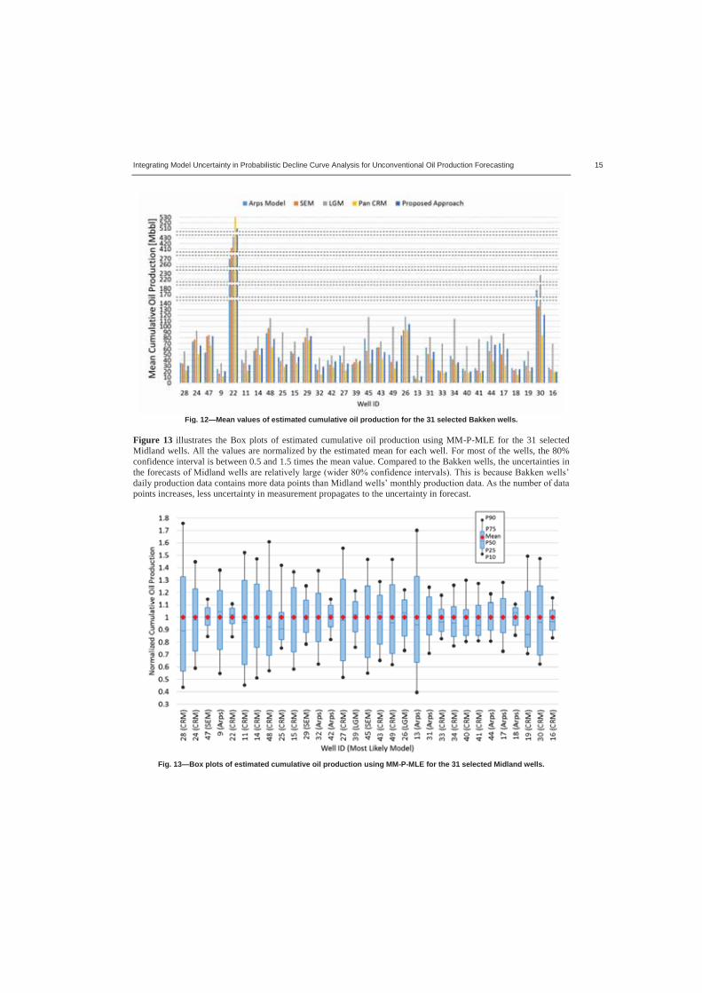
Integrating Model Uncertainty in Probabilistic Decline Curve Analysis for Unconventional Oil Production Forecasting 15
Fig. 12 Mean values of estimated cumulative oil production for the 31 selected Bakken wells.
Figure 13 illustrates the Box plots of estimated cumulative oil production using MM-P-MLE for the 31 selected Midland wells. All the values are normalized by the estimated mean for each well. For most of the wells, the 80% confidence interval is between 0.5 and 1.5 times the mean value. Compared to the Bakken wells, the uncertainties in the forecasts daily production data contains more data points than Midland wpoints increases, less uncertainty in measurement propagates to the uncertainty in forecast.
Fig. 13 Box plots of estimated cumulative oil production using MM-P-MLE for the 31 selected Midland wells.

Integrating Model Uncertainty in Probabilistic Decline Curve Analysis for Unconventional Oil Production Forecasting 16
Discussion Ambiguous choice of a single model for DCA can be caused by cognitive biases6. Overconfidence is one of the most common cognitive biases in the oil and gas industry (Welsh et al., 2005). When a single model is selected for DCA, one gives a 100% weight to this selected model (i.e., trust this model 100%). However, it is obvious that a single model should not be trust 100%. Thus, he/she is overconfident in the selected model. When diverse models are considered, the impact of overconfidence is reduced. Our proposed approach MM-P-MLE provides a consistent and systematic framework for including multiple models in probabilities DCA and updating the model probabilities/weights based on given data. Therefore, the risk of over/underestimate given by a single model is reduced and MM-P-MLE gives a moderate estimate.
Traditional measures of the goodness of fit (weighted) sum of squares and (weighted) can only be used to rank different models but they do not have any useful interpretation for probabilistic analysis. It is more useful for probability analysis to convert them into corresponding probability representation. Moreover, probability has a more intuitive interpretation to many people than sum of squares and .
The Pan CRM is the most likely model for most of the unconventional wells selected for this work. It tends to give the lowest estimate on cumulative oil production over long time among the four models studies in this work. This means that it is very likely that the true cumulative oil production is lower than the forecast by the other models
ate on future oil production has often turned out to be too optimistic.
However, no one model is best in all circumstances, as for some wells, the Arps, SEM or LGM models may performs better than the others. MM-P-MLE avoids the a priori choice of which model to use and the rejection of a possible good model. Thus, we are open-minded to other models and weights them according to their quality of data match. Any model holds the possibility to when the data provides enough evidence as more data becomes available.
When the number of data points is small, the model uncertainty remains large, because these data points do not clearly reflect the characteristics of different flow regimes of unconventional production. As the number of data points increases, the characteristics of different flow regimes is shown more clearly, and the model that cannot well capture the physics of all the flow regimes will be gradually eliminated (i.e., its probability approaches 0).
The Pan CRM is the only analytical model among the models we consider in this work. It is designed to capture the major flow regimes transient flow regime and semi-steady state flow regime involved in an unconventional well. Therefore, it is not surprising that the data from two unconventional fields show that the Pan CRM is the most likely one to well describe the flow behaviors, among the four models. Some wells show that one of the other three models is the most likely for some possible reasons: the measure errors masks the characteristics of different flow regimes, different flow regimes show up simultaneously, minor flow regimes appears, fracture flow is not dominating, or unclear flow behaviors appear. Besides, unlike that the parameters of an empirical model have no physical meaning, all the parameters of the Pan CRM are physically defined, and the fit parameter values reveal important reservoir/well properties. For example, the in the Pan CRM reveals the effective drainage volume of a producer.
Our investigation is limited to the Arps, SEM, LGM and Pan CRM models. More models should be included in this analysis. Other models (e.g., a dual-porosity reservoir simulation model) might be superior to the Pan CRM. However, we argue that using a more complex model with more parameters can make probabilistic analysis too computationally intensive and may not create much additional value (see the discussion in Bratvold and Begg (2009) and Hong et al. (2017)). One of the advantage of DCA is its speed. Thus, we prefer models with small number of parameters for DCA. Conclusions We propose an approach, MM-P-MLE, that integrates model uncertainty in probabilistic DCA for unconventional oil production forecasting. Different from the approach that uses only a single best-fit model for further analysis, the proposed approach interprets the goodness of fit of a model with a probability representation that can be carried to uncertainty analysis. The uncertainty in the Arps ( ), SEM and Pan CRM models for analyzing unconventional plays was investigated.
An example illustrated that the best-fit model may not be the model that best fits the flow behavior. Using the proposed approach can reduce the risk of using a best-fit but very wrong model for forecasting.
The proposed approach was applied with real oil production data from the Bakken and Midland fields. The hindcast test showed that the model uncertainty was reduced and the forecast was improved as more data points 6 A cognitive bias refers to the unconscious deviation from rationality in judgment (Haselton et al., 2005).

Integrating Model Uncertainty in Probabilistic Decline Curve Analysis for Unconventional Oil Production Forecasting 17
became available. The model probabilities were assessed and the cumulative oil productions were estimated using our proposed approach for 28 selected Bakken wells and 31 selected Midland wells. The proposed approach performed well in propagating the model uncertainty to the uncertainty in forecast. The results showed that:
It is confirmed that the Arps model ( ) may not be ideal for unconventional plays. The Pan CRM, as the only analytical model, is more likely to better describe the unconventional flow
behavior than the other three empirical models. No one model is the most likely for all wells. The model uncertainty can remain large even when the data length is long. The Arps and LGM models tends to give a larger estimate of the expected value of the cumulative oil
production than the other two models for the wells with small number of data points. Using the Aprs or LGM model with small number of data points may result in a too optimistic estimate in cumulative oil production.
By weighting the models, the proposed approach gives a moderate estimate of the cumulative oil production; neither too optimistic or too pessimistic.
Acknowledgements The authors acknowledge the support of the Research Council of Norway and industry partners: ConocoPhillips, Skandinavia AS, BP Norge AS, Det Norske Oljeselskap AS, Eni Norge AS, Maersk Oil Norway AS, DONG Energy A/S, Denmark, Statoil Petroleum AS, ENGIE E&P NORGE AS, Lundin Norway AS, Halliburton AS, Schlumberger Norge AS, and Wintershall Norge AS of The National IOR Centre of Norway.
Aojie Hong would like to thank the staffs and colleagues at the University of Texas at Austin for their support during his visiting. Larry W. Lake holds the Shahid and Sharon Ullah Chair at the University of Texas. References Arps, J. J. 1945. Analysis of Decline Curves. Transactions of the AIME 160 (1): 228 247.
https://doi.org/10.2118/945228-G. Bunn, D. W. 1975. A Bayesian Approach to the Linear Combination of Forecasts. Journal of the Operational
Research Society 26 (2): 325 329. http://dx.doi.org/10.1057/jors.1975.67. Bratvold, R. B., and Begg, S. H. 2008. I Would Rather be Vaguely Right than Precisely Wrong: a New Approach to
Decision Making in the Petroleum Exploration and Production Industry. AAPG bulletin 92 (10): 13731392. http://dx.doi.org/10.1306/06040808070.
Bratvold, R. B., and Begg, S. H. 2009. Would You Know a Good Decision if You Saw One? The Way Ahead 5 (2): 21 23. SPE-0209-021-TWA. https://doi.org/10.2118/0209-021-TWA.
Cheng, Y., Wang, Y., McVay, D., and Lee, W. J. 2010. Practical Application of a Probabilistic Approach to Estimate Reserves Using Production Decline Data. SPE Economics & Management 2 (1): 19 31. SPE-95974-PA. http://dx.doi.org/10.2118/95974-PA.
Clark, A. J., Lake, L. W., & Patzek, T. W. 2011. Production Forecasting with Logistic Growth Models. Society of Petroleum Engineers. Presented at the SPE Annual Technical Conference and Exhibition, Denver, USA, 30 October 2 November. SPE-144790-MS. http://dx.doi.org/10.2118/144790-MS.
Clemen, R. T., and Winkler, R. L. 1999. Combining Probability Distributions from Experts in Risk Analysis. Risk Analysis 19 (2): 187 203. http://dx.doi.org/ 10.1111/j.1539-6924.1999.tb00399.x.
Duong, A. N. 2011. Rate-Decline Analysis for Fracture-Dominated Shale Reservoirs. Society of Petroleum Engineers. SPE Reservoir Evaluation & Engineering 14 (3): 377 387. SPE-137748-PA. http://dx.doi.org/10.2118/137748-PA.
Dillon, R. L., John, R., and von Winterfeldt, D. 2002. Assessment of Cost Uncertainties for Large Technology Projects: a Methodology and an Application. Interfaces 32 (4): 52 66.
Gong, X., Gonzalez, R., McVay, D. A., and Hart, J. D. 2014. Bayesian Probabilistic Decline-Curve Analysis Reliably Quantifies Uncertainty in Shale-Well-Production Forecasts. SPE Journal 19 (6): 1047 1057. SPE-147588-PA. http://dx.doi.org/10.2118/147588-PA.
Gonzalez, R. A., Gong, X., and McVay, D. A. 2012. Probabilistic Decline Curve Analysis Reliably Quantifies Uncertainty in Shale Gas Reserves Regardless of Stage of Depletion. Presented at the SPE Eastern Regional Meeting, Lexington, USA, 3 5 October. SPE-161300-MS. http://dx.doi.org/10.2118/161300-MS.
Hong, A. J., Bratvold, R. B., and Nævdal, G. 2017. Robust Production Optimization with Capacitance-Resistance Model as Precursor. Computational Geosciences. https://doi.org/10.1007/s10596-017-9666-8.
Haselton, M. G., Nettle, D., and Murray, D. R. 2005. The Evolution of Cognitive Bias. The Handbook of

Integrating Model Uncertainty in Probabilistic Decline Curve Analysis for Unconventional Oil Production Forecasting 18
Evolutionary Psychology: 724 746. https://doi.org/10.1002/9781119125563.evpsych241. Ilk, D., Rushing, J. A., Perego, A. D., and Blasingame, T. A. 2008. Exponential vs. Hyperbolic Decline in Tight Gas
Sands: Understanding the Origin and Implications for Reserve Estimates Using Arps Decline Curves. Presented at the SPE Annual Technical Conference and Exhibition, Denver, USA, 21 24 September. SPE-116731-MS. http://dx.doi.org/10.2118/116731-MS.
Jouini, M. N., and Clemen, R. T. 1996. Copula Models for Aggregating Expert Opinions. Operations Research 44 (3): 444 457. http://dx.doi.org/10.1287/opre.44.3.444
Joshi, K., and Lee, W. J. 2013. Comparison of Various Deterministic Forecasting Techniques in Shale Gas Reservoirs. Presented at the SPE Hydraulic Fracturing Technology Conference, The Woodlands, USA, 4 6 February. SPE-163870-MS. http://dx.doi.org/10.2118/163870-MS.
Jochen, V. A., and Spivey, J. P. 1996. Probabilistic Reserves Estimation Using Decline Curve Analysis with the Bootstrap Method. Presented at the SPE Annual Technical Conference and Exhibition, Denver, USA, 6 9 October. SPE-36633-MS. http://dx.doi.org/10.2118/36633-MS.
Pan, Z. 2016. Revised Productivity Index Equation to Improve Transient History Match for the Capacitance Resistance Model. Master Thesis. The University of Texas at Austin, USA.
Read, C. 1920. Logic: Deductive and Inductive, reprinted. London, UK: Simkin. Stone, M. 1961. The Opinion Pool. The Annals of Mathematical Statistics 32 (4), 1339 1342.
http://dx.doi.org/10.1214/aoms/1177704873. Sayarpour, M., Kabir, C. S., Sepehrnoori, K., and Lake, L. W. 2011. Probabilistic History Matching with the
Capacitance Resistance Model in Waterfloods: a Precursor to Numerical Modeling. Journal of Petroleum Science and Engineering 78 (1), 96 108. https://doi.org/10.1016/j.petrol.2011.05.005.
Tavassoli, Z., Carter, J. N., and King, P. R. 2004. Errors in History Matching. SPE Journal 9 (3): 352 361. SPE-86883-PA. http://dx.doi.org/10.2118/86883-PA
Valko, P. P. 2009. Assigning Value to Stimulation in the Barnett Shale: a Simultaneous Analysis of 7000 plus Production Histories and Well Completion Records. Presented at the SPE Hydraulic Fracturing Technology Conference, The Woodlands, USA, 19 21 January. SPE-119369-MS. http://dx.doi.org/10.2118/119369-MS.
Valko, P. P., and Lee, W. J. 2010. A Better Way to Forecast Production from Unconventional Gas Wells. Presented at the SPE Annual Technical Conference and Exhibition, Florence, Italy, 19 22 September. SPE-134231-MS. http://dx.doi.org/10.2118/134231-MS
Welsh, M. B., Bratvold, R. B., and Begg, S. H. 2005. Cognitive Biases in the Petroleum Industry: Impact and Remediation. Presented at the SPE Annual Technical Conference and Exhibition, Dallas, USA, 9 12 October. SPE-96423-MS. https://doi.org/10.2118/96423-MS.
Wattenbarger, R. A., El-Banbi, A. H., Villegas, M. E., and Maggard, J. B. 1998. Production Analysis of Linear Flow into Fractured Tight Gas Wells. Presented at the SPE Rocky Mountain Regional/Low-Permeability Reservoirs Symposium, Denver, USA, 5 8 April. SPE-39931-MS. http://dx.doi.org/10.2118/39931-MS.

Paper II
Robust Production Optimization with Capacitance-Resistance Model as Precursor
Hong, A.J., Bratvold, R.B., and Nævdal, G.


Comput Geosci (2017) 21:1423–1442DOI 10.1007/s10596-017-9666-8
ORIGINAL PAPER
Robust production optimization with capacitance-resistancemodel as precursor
A. J. Hong1,2 · R. B. Bratvold1,2 · G. Nævdal1,3
Received: 13 October 2016 / Accepted: 24 May 2017 / Published online: 24 June 2017© Springer International Publishing Switzerland 2017
Abstract Many model-based techniques for optimizinghydrocarbon production, especially robust optimization(RO), carry prohibitive computational cost. Ensemble-basedoptimization (EnOpt) is a promising RO method but iscomputationally intensive when based on rich grid-basedreservoir models with hundreds of realizations. We presenta proxy-model workflow where a grid-based model issupplemented by a useful yet tractable proxy model. Acapacitance-resistance model (CRM) can be a proxy modelfor waterflooding systems. We illustrate the use of CRM-based models and investigate their pros and cons usingsynthetic 2D and 3D models. A selected proxy modelis embedded into the proxy-model workflow. The resultsobtained from the proxy-model and traditional workflowsare compared. The impact of any differences is assessedby considering a relevant decision-making context. Themain contributions are (1) a general RO workflow thatembeds proxy models, (2) a discussion of the desiderataof proxy models, (3) illustration and discussion of the useof CRM-based models in the proxy-model workflow, and
� A. J. [email protected]
R. B. [email protected]
G. Næ[email protected]
1 The National IOR Centre of Norway, Stavanger, Norway
2 Department of Petroleum Engineering, Universityof Stavanger, Stavanger, Norway
3 International Research Institute of Stavanger,Stavanger, Norway
(4) a discussion of the impact of using a proxy modelfor production optimization in a decision-making context.Based on our study, we conclude that CRM-based mod-els have high potential to serve as a cogent proxy modelfor waterflooding related decision-making context and thatthe proxy-model workflow, leveraging a faster, but relevant,production model, significantly speeds up the optimizationyet gives robust results that leads to a near-optimal solution.
Keywords Model-based hydrocarbon productionoptimization · Geological uncertainty · Robust productionoptimization · Ensemble-based optimization ·Computational cost · Grid-based reservoir model ·Capacitance-resistance model · Proxy model · Waterinjection · Decision-making · Value of verisimilitude
1 Introduction
The past few decades have seen rapid development innumerical techniques for model-based optimization of sub-surface hydrocarbon production (to optimize the reserves,the production over some time frame, the value of thereserves or production, etc.). However, these techniquestypically require computation for a numerous reservoir sim-ulations, especially for robust optimization (RO).
Within RO, the geological uncertainties are representedby a set of realizations (i.e., an ensemble). The objective ofRO is to find a control vector (e.g., a water injection scheme)that optimizes the expected value (EV) of the objectivefunction, such as net present value (NPV), given the geolog-ical uncertainties represented by the realizations. Hence, theoptimal solution is robust to geological uncertainties. vanEssen et al. [33] used RO to optimize hydrocarbon produc-tion under geological uncertainty, where an adjoint-based

1424 Comput Geosci (2017) 21:1423–1442
method is used for obtaining the gradient information. Theadjoint-based method requires access to the source codeof the reservoir simulator, which is seldom available forcommercial simulators, and it is computationally intensive.
Chen et al. [13] introduced the ensemble-based optimiza-tion method (EnOpt), in which the gradient is approximatedby the covariance between the objective function valuesand the control variables. Regardless of the type of reser-voir simulators, EnOpt is easier to implement than other ROmethods and is less computationally intensive [17]. Do andReynolds [15] analyzed the theoretical connections betweenEnOpt and other approximate gradient-based optimizationmethods. Having realized that it is unnecessary to approxi-mate the ensemble mean to the sample mean as was done byChen et al. [13], Do and Reynolds [15] used the ensemblemean in their EnOpt formulation.
Fonseca et al. [17] further modified Do and Reynolds’s[15] EnOpt formulation and found that the modified EnOptformulation1 both gives a better objective function value andconverges more quickly than the original EnOpt and othervariants of ensemble-based optimization method. Althoughit has been demonstrated that EnOpt (both the originalformulation and its variants) is a vast improvement overearlier optimization methods, it is nonetheless computation-ally intensive, typically involving thousands of reservoirsimulations [29]. The differences between the original andmodified EnOpt formulations will be stated in detail inSection 3.
Yang et al. [35] used a second order polynomial proxymodel to reduce the number of required simulations inRO. Denney [14] discussed the pros and cons of applyinga proxy model as a substitute for full reservoir simula-tions in assisted history matching, production optimizationand prediction, and found that proxy models do not givean optimal solution in many cases but are less compu-tationally demanding in finding improved solutions. Ourpaper presents an alternative, and general, workflow wherea grid-based reservoir model is supplemented by a material-balance-based proxy model for RO. This proxy model isintended to capture the range of possible production pro-files, yet be less computationally intensive than the reser-voir simulators currently used in EnOpt. Thus, the choiceand usefulness of a proxy model for this purpose willbe a function of the reservoir characteristics and drainagescheme. Our main focus is waterflooding systems for whichcapacitance-resistance model (CRM) is a potential candidate.
Bruce [9] applied the analogy of a capacitance-resistanceelectric network to analyzing reservoir and well behavior.Albertoni and Lake [1] introduced a model that combined
1We refer the EnOpt formulation modified by Fonseca et al. [17] to asthe modified EnOpt formation in the rest of the paper.
a multivariate linear regression analysis with diffusivity fil-ters and used only production and injection rate data toinvestigate the connectivity and response time between aproducer and an injector in a waterflooded reservoir. Gentil[18] showed that the connectivity is a function of transmis-sibilities. Yousef et al. [36] introduced CRM by modifyingAlbertoni and Lake’s work [1] to use the weight to quan-tify the connectivity and to employ the time constant toquantify the fluid storage within each injector-producer pair.Sayarpour [27] used superposition in time to analyticallysolve the numerical integration in CRM.
To overcome the original CRM’s limitation that the totalfluid flow is treated as a single phase, a CRM was combinedby Sayarpour et al. [28] with a Buckley-Leverett-basedfractional flow model, by Gentil [18] with an empiricalfractional flow equation, and by Cao et al. [12] with theKoval [22] model. Cao [10] demonstrated that the Kovalmodel might not yield a good match for mature waterfloodsbecause it might approach an abrupt end of 100% water cut.She also noted that the Gentil model might not work well forimmature waterfloods because the relationship between thenatural logs of water-oil ratio and cumulative water injectionmight be non-linear at that stage. These concerns promptedthe development of a fully coupled two-phase-flow-basedCRM, which is applicable in all stages of maturity [10, 11].
To allow for the inherent uncertainty in history match-ing [31], Sayarpour et al. [28] started with different setsof initial guesses of unknown CRM parameters and usedproduction data to generate numerous history-matched solu-tions of CRM. Jafroodi and Zhang [21] applied a CRMin a closed loop consisting of ensemble Kalman filter(EnKF) and EnOpt to capture the geological uncertaintiesand the time-variance of the CRM parameters. CRM hasbeen shown to be quite accurate for waterflooding systemsand used as a tool for waterflood production optimization[24, 30].
The above studies on CRM employed it in the productionphase with real production data (in the synthetic studies, the“real” production data is mimicked by the synthetic modelsimulated production data). In the proxy-model workflow,we do not need any real production data for using CRMbecause the CRM is history-matched to grid-based modelsimulated production data (i.e., pseudo production data).Thus, the proxy-model workflow can be used when realproduction data is unavailable (e.g., in the design phase).
In Section 2, we review two CRM-based models, a CRMcombined with the Koval model (the CRMP-Koval Model)and the fully coupled two-phase flow based CRM (the Cou-pled CRMP). Section 3 gives a short introduction on RO andEnOpt. Section 4 illustrates the proxy-model workflow. InSections 5 and 6, this workflow is tested in two examples;one with a 2D reservoir simulation model and the other witha 3D model. The matching qualities of the two CRM-based

Comput Geosci (2017) 21:1423–1442 1425
models are compared for screening purposes in the 2Dmodel example. The selected proxy model is embedded intothe proxy-model workflow. The results of the proxy-modeland traditional workflows are contrasted and discussed. Fur-thermore, the impacts of these results are investigated in adecision-making context. Finally, we present a discussionand conclusions in Sections 7 and 8, respectively.
The main contributions of this work are (1) a general ROworkflow embedding proxy models, (2) a discussion of thedesiderata of proxy models for production optimization, (3)illustration and discussion of the use of CRM-based modelsin the proxy-model workflow, and (4) a discussion of theimpact of using a proxy model for production optimizationin a decision-making context.
2 Capacitance-resistance model
A capacitance-resistance model (CRM) is based on mate-rial balance and derived from total fluid continuity equation.It contains considerably fewer parameters and needs sig-nificantly less computation time than does a grid-basedreservoir model. Required input data for a CRM are pro-duction rates, injection rates, and producers’ Bottom-HolePressures (BHP). The two main parameters of a CRM areconnectivity and time constant. For an oil-water system,connectivity is the proportion of injected water in an injectorthat contributes to the total fluid production in a producer.The time constant indicates how long a pressure wave froman injector takes to reach a producer.
Based on control volume, CRM can be divided intothree categories: single-tank CRM (CRMT), producer-based CRM (CRMP), and injector-producer-pair-basedCRM (CRMIP) [30]. As illustrated in Fig. 1, the controlvolume in a CRMT is the entire drainage volume of a reser-voir covering a single pseudo-producer (encompassing allphysical producers) and a single pseudo-injector (encom-passing all physical injectors), enabling the entire reservoirto be treated as a single tank with one inlet and one out-let. A CRMP has producer-based control volumes, each ofwhich covers all the injectors influencing its correspond-ing producer. A CRMIP has one control volume for eachinjector-producer pair. Because the original CRM [36] canpredict only total fluid production, it must be combined witha fractional flow model in order to separate oil productionfrom the total production. In the following, we review twoCRMP-based models for the case of an oil-water systemunder waterflooding and constant producer BHPs.
2.1 The CRMP-Koval Model
The Koval factor [22] was introduced into the Buckley-Leverett fractional flow equation in order to capture the
fingering effect induced by heterogeneity and the unfavor-able mobility ratio between the displacing and displacedfluids. Cao et al. [12] illustrated how CRMP combinedwith the Koval fractional flow equation (the CRMP-KovalModel) can be used to forecast oil and water productionunder waterflooding. For constant producer BHPs, the totalfluid production equation of CRMP is [27]
qtkj = qt
k−1j e−�tk/τj + (1 − e−�tk/τj )(
ninj∑i=1
λij Iki ), (1)
where sub/superscripts i, j , and k are the indices of injector,producer, and time step, respectively; qt
kj is the total fluid
production rate of producer j at time k; �tk is the time steplength between times k and k − 1; τj is the time constantfor producer j ; ninj is the number of injectors; λij is theconnectivity between injector i and producer j ; and I k
i is thewater injection rate of injector i during the period of �tk .Both λ and τ are assumed to be constant with respect to time[12].2
Cao et al. [12] used the following form of the Kovalfractional flow equation:
fwkj =
⎧⎪⎪⎨⎪⎪⎩0, if tDj < 1
Kvalj
Kval j −√Kvalj /tDj
Kval j −1 , if 1Kvalj
≤ tDj ≤ Kvalj
1, if tDj > Kvalj
, (2)
where
tDj =∑nT
k=1 Itkj
Vpj
, (3)
fwkj is the water cut in producer j at time k, Kvalj is the
Koval factor of producer j , tDj is the dimensionless time orthe fraction of cumulative water injected into the drainagepore volume of producer j , nT is the number of time steps,It
kj is the total water injection contribution from all injectors
to producer j during �tk , and Vpjis the drainage pore vol-
ume of producer j . Assuming that the water injection rateof an injector is constant over �tk and equal to I k
i , Itkj can
be calculated by
Itkj = (
ni∑i=1
λij Iki )�tk. (4)
Thus, using the CRMP and the Koval fractional flow equa-tion, the water and oil production rates in producer j at timek (qw
kj and qo
kj ) are calculated, respectively, by
qwkj = qt
kj fw
kj , (5)
qokj = qt
kj (1 − fw
kj ). (6)
2This is equivalent to assuming no dramatic changes in reservoir orwell conditions.

1426 Comput Geosci (2017) 21:1423–1442
Fig. 1 Illustration of a CRMT,b CRMP, and c CRMIP
In the CRMP-Koval Model, the model parameters are theconnectivity λ of each injector-producer pair; and the timeconstant τ , the Koval factor Kval , and the drainage pore vol-ume Vp of each producer. These parameters are determinedby solving the least squares problem
minτj ,λij ,Kval j ,Vpj
z =nT∑k=1
np∑j=1
[(qtkj −qt
kj
obs)2+(qo
kj −qo
kj
obs)2]
(P1)
subject to
τj ≥ 0, (P1C1)
λij ≥ 0, (P1C2)
Kvalj ≥ 1, (P1C3)
np∑j=1
Vpj≤ VpField
, (P1C4)
np∑j=1
λij
{< 1, if injection loss exists= 1, if no injection loss
(P1C5)
where the superscript obs denotes the observed productiondata, np is the number of producers, and VpField
is thetotal pore volume of the field. For an optimization program,a different equation numbering system is used, where “P”denotes a program and “C” denotes a constraint. For exam-ple, Eq. P1C5 means constraint number 5 for optimizationprogram 1. For the case with aquifer support, Izgec andKabir [20] proposed coupling an aquifer model with a CRM.Because no aquifer is considered in the reservoir modelsused in the following examples, the effect of an aquiferwill not be considered in this paper. The total pore volumeof the field VpField
is defined by the total pore volume ofthe reservoir simulation model because in the proxy-modelworkflow, the observed production data are obtained fromreservoir simulation using the commercial black oil simula-tor ECLIPSETM [16], and the CRM is used to approximatethe reservoir simulation model. When VpField
is unknown,
such as when the CRM is used to match real productiondata, constraint Eq. P1C4 can be removed.
2.2 The Coupled CRMP
Cao et al. [11] developed the Coupled CRMP: a fully cou-pled two-phase flow model based on CRMP. In addition tothe total fluid balance equation (i.e., the pressure or continu-ity equation), they considered the oil mass balance equation(i.e., the saturation equation). This model can calculate theaverage saturation within a producer-based control volume,the outlet saturation of a producer, and the time-variant timeconstant. The following shows only the numerical solu-tion to the saturation equation. For more details on thederivation, see [10, 11].
Cao et al. [11] derived the semi-analytical explicit solu-tion to the saturation equation as
Sok
j =Sok−1j − �tk
Vpj
⎛⎝Sok−1j (cf + co)
ct
(∑i
λij Ikj − qt
kj
)+ qo
kj
⎞⎠ ,
(7)
where Sok
j is the average oil saturation within the controlvolume of producer j at time k, and cf , co, and ct are thepore, oil, and total compressibilities, respectively. Assum-ing that the major contribution to oil saturation change isfrom oil production rather than the effect of compressibil-ity [23], Cao [10] eliminated the compressibility term in thesaturation equation and derived a simplified solution as
Sok
j = Sok−1j − �tk
Vpj
qokj . (8)
We will be using Eq. 8 rather than Eq. 7. Cao [10] proposedusing the Welge equation [10, 23, 34] to calculate the outletoil saturation of a producer as
So2kj = So
k
j +∑nT
k=1 Itkj
Vpj
(1 − fwkj ), (9)
where So2kj is the outlet oil saturation of producer j at time
k.

Comput Geosci (2017) 21:1423–1442 1427
Using the definition of the time constant,
τ kj = Vpj
ct
Jtkj
, (10)
where Jtkj is the total productivity index of producer j at
time k, Eq. 10 can be rewritten as
τ kj = Tj
Mkj
, (11)
where
Tj = Vpjct
J′t j
, (12)
Mkj = kro(So2
kj )
μo
+ krw(So2kj )
μw
. (13)
Because J ′t j is assumed to be constant, Tj is time-invariant
[11]. The total relative mobility Mkj is time-variant because
it depends on the oil and water relative permeabilities, kro
and krw, which are functions of the outlet saturation. The oiland water viscosities, μo and μw, are assumed to be con-stant. It should be noted that the time constant is assumed tobe time-invariant in the CRMP-Koval Model, whereas it istime-variant in the Coupled CRMP. Thus, the time-invarianttime constant τj in the solution of the total fluid continuityequation (1) is replaced by the time-variant time constantτ kj , giving
qtkj = qt
k−1j e
−�tk/τkj + (1 − e
−�tk/τkj )
(ninj∑i=1
λij Iki
). (14)
The model parameters can be determined by solving theleast squares problem
minTj ,λij ,So
0j ,Vpj
z =nT∑k=1
np∑j=1
(qtkj − qt
kj
obs)2 (P2)
subject to
Tj ≥ 0, (P2C1)
λij ≥ 0, (P2C2)
Sor ≤ Sok
j , (P2C3)
So2kj ≤ 1 − Swi, (P2C4)
np∑j=1
Vpj≤ VpField
, (P2C5)
np∑j=1
λij
{< 1, if injection loss exists= 1, if no injection loss
(P2C6)
where So0j is the initial average oil saturation of producer
j , Sor is the residual oil saturation, and Swi is the irre-ducible water saturation. For the Coupled CRMP, the modelparameters are determined by matching only the total fluidproduction data. This is because the water cut fw
kj in Eq. 9
can be directly obtained from the production data. The frac-tional flow model is constructed using the water cut dataplotted against the average oil saturation calculated from theCoupled CRMP. Cao [10] used a polynomial function ofdegree 3 to fit the fractional flow curve based on the histori-cal data. We construct the fractional flow curve using a datatable consisting of existing water cut data against the calcu-lated average oil saturation from the Coupled CRMP at eachtime for each producer.
Using the Coupled CRMP for production prediction isnot as straightforward as using the CRMP-Koval Modelbecause production rates and saturations at any given timeare mutually dependent. In order to predict production withminimal errors, production rates and saturations have to besolved implicitly with iterations. For more details on theiterative algorithm, see [10]. For a given predicted averageoil saturation, the water cut can be predicted by extrapo-lation or interpolation of the water cut against average oilsaturation table constructed earlier. We use linear extrapola-tion or interpolation to find the corresponding water cut fora given average oil saturation, based on the data in the table.
3 Robust optimization (RO) of production
RO is performed over an ensemble of realizations represen-ting the geological uncertainties. For a risk-neutral decision-maker, the objective of RO is to optimize the EV over ofthe ensemble. The purpose of production optimization is tomaximize the NPV. Assuming that all revenues are from oilproduction and that all costs are induced by water injec-tion and water production, the objective function for a singlerealization can be defined as
J (u) = NPV (u)
= ∑nT
k=1(qk
o (u)Po−qkw(u)Pwp−I k(u)Pwi)�tk
(1+b)tk/D ,(15)
where u is the control vector (i.e., a vector of control vari-ables) defined as u = [u1, u2, ..., uN ]T, where N is thenumber of control variables; qk
o is the field oil productionrate at time k; qk
w is the field water production rate at timek; I k is the field water injection rate at time k; Po, Pwp,and Pwi are the oil price, water production cost, and waterinjection cost, respectively; b is the discount factor; tk isthe cumulative time for discounting; and D is the referencetime for discounting (D = 365 days if b is expressed as afraction per year and the cash flow is discounted daily). If

1428 Comput Geosci (2017) 21:1423–1442
a case involves multiple realizations, the objective functionbecomes
J (u) =∑ne
r=1 Jr(u)
ne
, (16)
where J is the EV of the objective functions over all realiza-tions, Jr is the objective function (15) of a single realizationr , and ne is the number of realizations (i.e., ensemble size).
EnOpt method can significantly reduce the number ofsimulations required for gradient calculation and can be eas-ily implemented with any type of simulator. In the originalEnOpt, the ensemble of values for control vector u1 u2 ...uM , where M is the ensemble size,3 is generated from amultivariate normal distribution with predefined mean u andpredefined covariance matrix Cu, which is used to specifythe temporal correlation of the controls to limit the fre-quency of changes in the controls. The predefined mean ucan be approximated by its sample mean u, i.e.,
u ≈ u =∑M
r=1 ur
M, (17)
and the average objective value J (u) can be approximatedby
J (u) =∑M
r=1 Jr (u)
M≈
∑Mr=1 Jr(ur )
M. (18)
Chen et al. [13] used these two approximations to calculatethe mean-shifted ensemble matrix U and the mean-shiftedobjective function vector j, respectively. However, Do andReynolds [15] did not find any advantage, theoretical orpractical, in approximating these two terms. Hence, themean-shifted ensemble matrix should be calculated directlyusing the predefined mean u by
U = [u1 − u, u2 − u, ..., uM − u]T. (19)
Moreover, Fonseca et al. [17] suggested calculating themean-shifted objective function vector with respect to theobjective value of the predefined mean for each individualrealization instead of the average objective value (18), i.e.,
j = [J1(u1) − J1(u), J2(u2) −J2(u), ...,
JM(uM) − JM(u)]T.(20)
The cross-covariance matrix is then
CuJ = 1
M(U
Tj). (21)
Chen et al. [13] approximated the gradient by
g ≈ CuJ. (22)
3M = ne if each realization is coupled with one sample of values forthe control vector, i.e., a 1:1 ratio is applied, as in our case.
For each iteration, the control vector is updated as
ul+1 = ul + αl
gl∥∥gl
∥∥∞, (23)
where the subscript l denotes the iteration number and α isthe step length for updating. Equations 19–23 constitute themodified EnOpt formulation [17]. The original EnOpt for-mulation can be obtained by replacing u with u in Eq. 19and Jr (u) with the approximated J (u) in Eq. 20. Fonsecaet al. [17] showed that the modified EnOpt converges toa higher objective value and more quickly than does theoriginal EnOpt. Therefore, we use the modified EnOpt.The step length α significantly affect convergence speed. Anaive line search procedure is to simply reduce α by half ifJ (ul+1) < J (ul). We use an interpolation-based line searchprocedure to find a relatively large value of α that satisfiesthe Armijo condition [26]. The line search procedure haltswhen J (ul+1) > J (ul) or after seven iterations, whichevercomes first. The modified EnOpt halts after 30 iterationsof control vector updating. In our case, an optimal solutionis found during the first 5–15 iterations. However, we con-tinue to iteration 30 in order to observe a clear evidence ofconvergence.
4 The proxy-model workflow
When geological uncertainty is considered and is repre-sented by hundreds of realizations, EnOpt usually requiresthousands of production prediction runs. In the traditionalworkflow, production is predicted by running grid-basedreservoir simulation. The computational intensiveness ofa grid-based reservoir model can be reduced by having aproxy model serve as a precursor. A proxy model must beable to serve our purpose (i.e., useful), and its computationaltime must be low (i.e., tractable). See the Discussion sectionfor the descriptions of “useful” and “tractable”. Figure 2depicts the traditional and proxy-model workflows.
A proxy model should be chosen based on the reser-voir characteristics and drainage scheme. More than onepotential proxy models may be found. For example, weconsider two CRM-based models for waterflooding. Thus,we need to screen these potential proxy models by testingtheir qualities of matching and prediction. ‘Pseudo pro-duction data” are generated by reservoir simulation thatincludes a random injection scheme.4 A history-matchingprocess is used to tune the parameters of a proxy model towhere the production predicted by the proxy model fits the
4We use the term “pseudo production data” because the data aresimulated rather than measured.

Comput Geosci (2017) 21:1423–1442 1429
Fig. 2 The traditional and proxy-model workflows
pseudo production data. The production predicted by thehistory-matched proxy model is then compared to that ofthe grid-based reservoir model, using another random injec-tion scheme. If the difference is unacceptably large either atthe history-matching step or at the validation step, we testanother potential proxy model. If the difference is small atboth steps, we use the proxy model for production optimiza-tion. After using the optimization algorithm with the proxymodel, we run simulation again on the grid-based reservoirmodel with the optimal control vector of the proxy model toget the final results (e.g., NPV). We conduct the last step forevaluating the optimal control vectors of the reservoir sim-ulation and proxy models on the same basis. This will bediscussed later.
5 Example with a 2D reservoir model
5.1 Description of the 2D reservoir model
This example uses a synthetic 2D reservoir model (“2DModel”) to test the CRM-based models and the proxy-model workflow. The 2D Model is an isotropic heteroge-neous model with four injectors and one producer in afive-spot pattern. The heterogeneity pertains to permeabil-ity only. Figure 3 shows the permeability field in millidarcy(md) and well locations of the model. The producer BHPsare fixed at 200 bars. The control variables are injectionrates for 50 time intervals of 30 days each (i.e., a life cycleof 1,500 days). For this specific example, the injection ratesof all injectors for a given day are assumed to be identical.Thus, there are 50 control variables.
5.2 Screening of the CRM-based models
This section examines the suitability of the CRMP-KovalModel and the Coupled CRMP for the proxy-model work-flow. However, this screening process is not limited toCRM-based models. For example, we can screen and com-pare a CRM-based model to other useful and tractablemodels such as the Interwell-Numerical-Simulation Model(INSIM) [37].
Model parameter determination and matching qualityWe determine the parameters of a proxy model by solving aleast squares problem using the interior-point optimizationalgorithm in MATLABTM [25]. Holanda et al. [19] intro-duced a matrix structure for the CRM representation thatdoes not need the analytical equation (1) for solving the leastsquares problem using MATLAB. Solving the least squaresproblem is actually a history-matching process because weminimize the difference between the production profilespredicted by the grid-based reservoir model and the proxy
Fig. 3 Illustration of the 2D model and its permeability field (indi-cated by the colors) for the deterministic case. All values are in md

1430 Comput Geosci (2017) 21:1423–1442
Fig. 4 Random well injection scheme for matching, 2D modelexample
model given an injection scheme. The well injection ratesare randomly generated from 0 to 200 m3/day (Fig. 4). Thecloseness of matching is depicted in Figs. 6 and 7 and isquantified by the coefficient of determination R2, defined as
R2 = 1 −∑
k(dobsk − d
prok )2∑
k(dobsk − d
obs)2
, (24)
where dobsk is the observed production data (the production
predicted by the grid-based reservoir model in our case)at time k, d
prok is the production predicted by the proxy
model at time k, and dobs
is the mean of dobsk over all k.
The closer R2 to 1, the better the matching. The values ofR2 are listed in Table 1. Both proxy models give almostequally good matches of total fluid production rate. TheCoupled CRMP matches water cut better than the CRMP-Koval Model because Koval model gives an abrupt end of100% water cut for mature waterflood (i.e., when watercut is high), as shown in Fig. 7 and demonstrated in [10,11]. Therefore, we choose the Coupled CRMP for furtherapplication.
Model validation and prediction quality Good matchingquality does not guarantee good prediction quality. Thissection will investigate whether the history-matched cou-pled CRMP can provide a production prediction close tothat of the 2D Model when the injection scheme is changed.We generate a new random injection scheme as shown in
Table 1 R2 of matching, deterministic case, 2D model example
Total production rate Water cut
CRMP-Koval 0.9998 0.9847
Coupled CRMP 0.9999 0.9999
Fig. 5 Random well injection scheme for validation, 2D modelexample
Fig. 5. The history-matched Coupled CRMP can providehighly accurate prediction in total production rate, with anR2 of 0.9998, and satisfactory prediction in water cut, withan R2 of 0.9984, as illustrated in Figs. 8 and 9, respectively.
Run time The computational time required for productionprediction was around 4.1 s for the 2D Model by ECLIPSEbut only around 0.17 s for the coupled CRMP by MATLAB.That is, the run time of production prediction is reducedby a factor of 24 by using Coupled CRMP instead of grid-based model. The run time of a grid-based reservoir modelis highly dependent on the number of grid blocks, num-ber of wells, and geological complexity, whereas the runtime of a CRM-based model depends on only the number ofwells and model chosen (CRMT, CRMP or CRMIP). Thus,a finer and/or more geologically complex grid-based reser-voir model will have a run time more than 24 times greaterthan that of its corresponding CRM-based model.
The shorter run time of the coupled CRMP enables fasterproduction prediction than using the 2D Model. Therefore,the run time of production optimization will be significantlyreduced if we use the Coupled CRMP instead of the 2DModel for RO.
Fig. 6 Matching of total fluid production rate, 2D model example

Comput Geosci (2017) 21:1423–1442 1431
Fig. 7 Matching of water cut, 2D model example
5.3 Life-cycle production optimization
We embed the Coupled CRMP into the proxy-model work-flow to serve as a proxy for production optimization. Weconsider two cases: a deterministic case where the perme-ability field of the grid-based reservoir model is certain, anda stochastic case where the permeability is uncertain andrepresented by an ensemble. For both cases, we optimizeNPV for 50 time steps of 30 days each, yielding a periodof 1,500 days. In order to get a well-constructed fractionalflow curve for the Coupled CRMP, we extend the reservoirsimulation to 3,000 days for determining the model param-eters so that the full range (0 to near 1) of water cut can becovered. For NPV calculation, the oil price, water produc-tion cost, water injection cost, and discount rate are set to315 $/m3, 47.5 $/m3, 12.5 $/m3, and 8%, respectively.
The deterministic case The grid-based reservoir modelused for this case is the single geological realizationdescribed earlier (Fig. 3). The model parameters of the Cou-pled CRMP are determined by matching the production datasimulated by the 2D Model. The matching quality is shownin Figs. 6 and 7. The history-matched Coupled CRMP isthen validated by contrasting its production prediction to
Fig. 8 Prediction of total fluid production rate, 2D model example
Fig. 9 Prediction of water cut, 2D model example
that of the 2D Model given a new injection scheme. Theprediction quality is shown in Figs. 8 and 9.
The well injection rate is constrained from 0 to 200m3/day. As a base case, the well injection rate is set to 100m3/day for the whole period of production.
Table 2 lists the base case NPV, the optimal NPV of theCoupled CRMP, and the solutions obtained using the tradi-tional and proxy-model workflows. Figure 10 illustrates theoptimal injection schemes of the Coupled CRMP and the2D Model. For the 2D Model and the Coupled CRMP underthe optimal injection scheme of the Coupled CRMP, Fig. 11shows the predicted total fluid production rate and Fig. 12shows the water cut. These results indicate that the CoupledCRMP again provides an accurate prediction, with an R2
of 0.9998 for total production rate and an R2 of 0.9968 forwater cut.
Compared to the 2D Model, the Coupled CRMP under-estimates NPV ($31.960 million vs. $32.406 million) forthe same injection scheme. The results show that the proxy-model workflow (i.e., applying the optimal strategy from theCoupled CRMP to the 2D Model) can provide an optimalNPV ($32.406 million) very close to that of the tradi-tional workflow ($32.902 million). Figure 10 shows that theproxy-model and traditional workflows result in differentoptimal injection schemes. This is due to the stochastic fea-ture of EnOpt and/or the approximation of the proxy modelto the grid-based reservoir model.
Table 2 NPVs [$ million], deterministic case, 2D model example
Model Base case Optimal Improvement
Coupled CRMP 23.767 31.960 34.47%
2D Model 24.476 32.406a,b 32.40%
2D Model 24.476 32.902c 34.43%
aWith optimal injection scheme of the Coupled CRMPbThe solution of the proxy-model workflowcThe solution of the traditional workflow

1432 Comput Geosci (2017) 21:1423–1442
Fig. 10 Optimal injection schemes of the 2D Model and the CoupledCRMP, deterministic case
To further compare the Coupled CRMP with the 2DModel, we depict in 3D their objective function spacesusing multi-dimensional scaling (MDS) [4, 17]. MDS canproject a set of high-dimensional vectors onto a 2D spaceaccording to the Euclidean distance between any two ofthem. In the 3D plot, the control vectors are projected onthe x-y plane, and the objective function values (i.e., NPV)are on the z-axis. Because the objective function actuallyoccupies a high-dimensional space, errors in the Euclideandistances and overlaps of vectors can occur in the 3D plot.Nevertheless, the 3D plot provides useful insights into theoptimization problem.
Each 3D plot of the objective function space consists of100 samples of normally distributed control vectors arounda central point (either the optimal injection scheme of theCoupled CRMP or of the 2D Model), with a standard devi-ation of 1/10 of the difference between the upper bound(200 m3/day) and the lower bound (0 m3/day). In Figs. 13,14, 15, and 16, the red dots represent the optimal controlvector either of the Coupled CRM or of the 2D Model,the rings represent the random control vectors, and the big
Fig. 11 Total fluid production rate under the optimal injection schemeof the Coupled CRMP, deterministic case, 2D model example
Fig. 12 Water cut under the optimal injection scheme of the CoupledCRMP, deterministic case, 2D Model example
blue dots represent the control vector corresponding to thehighest NPV among all the samples. Figures 13 and 14 havethe same random control vectors and thus the same projec-tion on the x-y plane. The same applies to Figs. 15 and 16.However, the control vectors and projection of Figs. 13and 14 are different from that of Figs. 15 and 16.
Comparing Figs. 13 to 14 and Figs. 15 to 16 confirms thatthe objective function spaces of the Coupled CRMP and the2D Model differ because of approximating the 2D Modelwith the Coupled CRMP. However, they share some com-mon features. For example, the locations of some of theirpeaks and valleys are the same. Figure 13 shows that, on theCoupled CRMP, EnOpt leads to a higher NPV than all thesample vectors around it, indicating that it might be a globaloptimum (at least in the control vector space around theoptimum found). However, for the 2D Model, Fig. 14 showsthat some control vectors can have a higher NPV than theoptimal control vector of the Coupled CRMP. Given that thedifferences between the highest and lowest values are only1.2% and 2.3% in Figs. 13 and 14, respectively, the spacescan be considered plateaus with small bumps. Performing
Fig. 13 Objective function space of the Coupled CRMP around theoptimal control vector of the Coupled CRMP, deterministic case, 2Dmodel example

Comput Geosci (2017) 21:1423–1442 1433
Fig. 14 Objective function space of the 2D Model around the optimalcontrol vector of the Coupled CRMP, deterministic case, 2D modelexample
EnOpt on the Coupled CRMP brings us to the plateau ofthe 2D Model’s objective function space, but to a bump thatis somewhat lower than the highest. In Fig. 15, the optimalcontrol vector of the 2D Model has the highest NPV amongall the sample vectors, indicating that it might be a globaloptimum. The optimal control vector of the 2D Model alsodoes not lead to an optimal NPV on the Coupled CRMP, asshown in Fig. 16.
Figure 17 illustrates the objective function values of the2D Model vs. that of the Coupled CRMP, where the bluedots correspond to the control vector samples in Figs. 13and 14, and the red dots do likewise for Figs. 15 and 16.The Coupled CRMP is shown to underestimate NPV with alargest difference of 3.8% for all the samples. This is why,in the proxy-model workflow, we estimate NPV on the 2DModel again after we have obtained the optimal control ofthe Coupled CRMP.
The stochastic case In order to consider the uncer-tainty in permeability, we generate 100 realizations of the
Fig. 15 Objective function space of the 2D Model around the optimalcontrol vector of the 2D Model, deterministic case, 2D model example
Fig. 16 Objective function space of the Coupled CRMP around theoptimal control vector of the 2D Model, deterministic case, 2D modelexample
permeability field from a multivariate normal distribution.Three of these realizations are shown in Fig. 18. Thematching procedure Eq. P2 is repeated for all the real-izations, yielding 100 sets of the parameters of the Cou-pled CRMP (i.e., an ensemble of the Coupled CRMP).The injection schemes for matching and validation in thiscase are the same as those used for the deterministic case(Figs. 4 and 5). The qualities of matching and predictionare shown in Figs. 19 and 20, respectively. The match-ing quality is good: the minimal R2 (the worst matching)for total production rate and water cut are 0.9950 and0.9929, respectively. The prediction quality is not as goodas the matching quality, but still satisfactory with a mini-mal R2 of 0.9946 for total production rate and 0.9546 forwater cut.
For robust production optimization, we use EnOpt tomaximize the expected NPV over all the realizations undera single injection scheme. The starting point uses an injec-tion rate of 100 m3/day for all the producers and time steps.The optimal expected NPV of the 2D Model is $32.031million and of the Coupled CRMP is $31.124 million. The
Fig. 17 Objective function values of the 2D Model vs. the CoupledCRMP, deterministic case

1434 Comput Geosci (2017) 21:1423–1442
Fig. 18 Three realizations of the permeability field, stochastic case, 2D model example
Fig. 19 Matching of total fluidproduction rate and water cut,stochastic case, 2D modelexample. a total fluid productionrate from the 2D Model, b watercut from the 2D Model, c totalfluid production rate from theCoupled CRMP, and d water cutfrom the Coupled CRMP
Fig. 20 Validation of total fluidproduction rate and water cut,stochastic case, 2D modelexample. a total fluidproduction rate from the 2DModel, b water cut from the 2DModel, c total fluid productionrate from the Coupled CRMP,and d water cut from theCoupled CRMP

Comput Geosci (2017) 21:1423–1442 1435
Table 3 Expected NPVs [$ million], stochastic case, 2D modelexample
Model Base case Optimal Improvement
Coupled CRMP 22.961 31.124 35.55%
2D Model 23.624 31.837a,b 34.76%
2D Model 23.624 32.031c 35.59%
aWith optimal injection scheme of the Coupled CRMPbThe solution of the proxy-model workflowcThe solution of the traditional workflow
expected NPV of the proxy-model workflow is $31.837million, which is close to that of the traditional workflow.Table 3 lists the expected NPVs. Figure 21 illustrates thecumulative distribution functions (CDF) of NPV corre-sponding to the optimal solutions of the 2D Model and ofthe Coupled CRMP, and to the 2D Model under the opti-mal injection scheme of the Coupled CRMP. The optimalinjection schemes are shown in Fig. 22.
As was found in the deterministic case, the proxy-modeland traditional workflows lead to similar optimal expectedNPVs, but to different optimal injection schemes and hencedifferent NPV distributions (the solid red curve vs. the solidblue curve in Fig. 21). Again, the Coupled CRMP underes-timates NPV (the dashed red curve vs. the solid red curve inFig. 21). The shapes of the cumulative distribution functions(CDF) of NPV are very similar.
The total number of production prediction runs duringEnOpt was 21,800 for the Coupled CRMP and 15,600 forthe 2D Model. The run times of the Coupled CRMP andthe 2D Model for a prediction of 3,000 days were 0.17and 4.1 s, respectively, and the computational time of onehistory matching was 1.1 s. The 1,500-day run time of a life-cycle prediction is one half of the run time of a 3,000-dayprediction. The total computational time of the traditionalworkflow is
Fig. 21 CDF of NPV, stochastic case, 2D model example
Fig. 22 Optimal injection schemes, stochastic case, 2D modelexample
Time for optimization
= 15, 600 × 4.12 = 31, 980 [s],
and of the proxy-model workflow is
(Time for matching) + (time for optimization)+ (time for expected NPV calculation)
= 100 × (4.1 + 1.1) + 21,800 × 0.172+ 100 × 4.1
2= 2,578 [s].
The computation time required by the proxy-model work-flow is therefore less than 1/10 that of the traditionalworkflow. The distinction will become more pronounced ifthe grid-based reservoir model has a finer grid block size orhigher geological complexity.
5.4 Impact on decision-making
This section explores the impact of any difference in opti-mal solutions obtained by the proxy-model and traditionalworkflows. We consider a simple decision-making contextthat involves three decisions in series. The first decision hastwo options: to continue developing the field at a cost of $10million or to walk away. The second decision is whether toinstall valves on the injectors at a cost of $2 million, giventhat water would be injected at a constant rate of 100 m3/dayover the entire production life-cycle without valves or at anyrate from 0 to 200 m3/day with valves. The third decisionis to choose a water injection scheme if valves are installed.All the decisions will be based on our current knowledgeabout the field. We assume a risk-neutral case where theobjective is to optimize the EV.
Figures 23 and 24 illustrate the decision trees for the solu-tions of the proxy-model and traditional workflows, respec-tively, for the deterministic case. In decision trees, a square,a circle, and a triangle represent a decision node, an uncer-tainty node, and a payoff node, respectively. (See [6] for adetailed description of using decision trees to solve hydro-carbon production related decision-making problems.) The

1436 Comput Geosci (2017) 21:1423–1442
Fig. 23 Decision tree with the optimal solution of the proxy-modelworkflow, deterministic case, 2D model example. All values are in $million
decision trees in Figs. 23 and 24 select the same decisionsfor the first and second decision nodes. However, the twoworkflows make the third decision diverge, resulting in arevenue of $20.406 million for the proxy-model workflow(applying the blue line in Fig. 10) and a revenue of $20.902million for the traditional workflow (applying the red line inFig. 10).
One reason of this difference is the stochastic feature ofEnOpt and the other is the verisimilitude or the richness5 ofthe models. If we adjust for the stochastic feature of EnOpt,the only difference between the proxy-model and traditionalworkflows is in the verisimilitude of the predictive modelused for production optimization. The proxy-model work-flow uses a model that is less rich but faster than that usedin the traditional workflow. To quantify the benefit thatthe verisimilitude might offer, we introduce the value ofverisimilitude (VOV), which is defined as
V OV = v(urich) − v(uproxy), (25)
where v(u) is the true value of the decision given a controlu, urich is the control vector found by using the traditionalworkflow, and uproxy is that found by the proxy-modelworkflow. However, being that a given field can supportonly one production strategy and can not yield the true valueuntil the end of production, the rich model is assumed to rep-resent the truth. The VOV of the deterministic case shownin Figs. 23 and 24 is $20.902 million – $20.406 million =$0.496 million. Similar to the statement for value of infor-mation (VOI) that “one cannot value information outside ofa particular decision context” [8], using a more verisimilarproduction prediction model has no value in itself, unless itchanges our decision. Thus, the 2D Model (a richer model)adds no value to the first and second decisions in this case.It adds value only to the third decision. The VOV is pos-itive because the 2D Model can capture more minor flowbehaviors than can the Coupled CRMP, giving a more accu-rate production prediction under our assumption that the
5This paper uses “richness” interchangeably with “complexity” and“verisimilitude” to indicate a high level of detail built into a model.
Fig. 24 Decision tree with the optimal solution of the traditionalworkflow, deterministic case, 2D model example. All values are in $million
2D Model represents the truth. However, the VOV ($0.496million), compared to the NPV improvement ($20.406 mil-lion − $14.476 million = $5.930 million) by installing thevalves and conducting the optimal injection scheme foundby performing EnOpt on the Coupled CRMP, is relativelysmall. This is because the Coupled CRMP is already a goodapproximation to the 2D Model.
For the stochastic case, the decision trees are illustrated inFigs. 25 and 26. The P10, P50, and P90 values are shown inthe decision trees. The distributions of the NPV are expectedto differ because the proxy-model and traditional work-flows lead to different optimal injection schemes. Given ourobjective of maximizing the expected NPV of a particulardecision-making problem, the solution of the proxy-modelworkflow gives an expected NPV very close to that of thetraditional workflow. This observation is consistent withthat in the deterministic case. To calculate the VOV, weassume that each realization of the 2D Model is equi-probable to be the truth. Hence, the VOV for one particularrealization is calculated as
V OV r = vr(urich) − vr(uproxy), (26)
where vr(u) is the value of the decision given a control vec-tor u if realization r of the rich model is the truth. Theexpected VOV (EVOV) is the EV of V OV r over all thegeological realizations. The EVOV is $20.031 million −$19.837 million = $0.194 million for the case shown inFigs. 25 and 26. The corresponding CDF of the VOV isillustrated in Fig. 27 and shows that there is around 5.4%chance of a negative VOV. The minimal VOV is −$0.096million, and the maximal is $0.783 million.
We investigate the sensitivity of EVOV to the valve costby varying the latter. The results are plotted in Fig. 28 whichcan be divided into three regions: valve cost lower than$8.21 million (Region 1), between $8.21 million and $8.41million (Region 2) and greater than $8.41 million (Region3). In Region 1, the EVOV is a constant $0.194 millionbecause only the third decision is affected by whether theproxy-model or traditional workflow is chose. In Region 2,installing valves is called for by the traditional workflow

Comput Geosci (2017) 21:1423–1442 1437
Fig. 25 Decision tree with theoptimal solution of the proxy-model workflow, stochasticcase, 2D model example
but not by the proxy-model workflow. In Region 3, EVOVdrops to 0 because neither the proxy-model nor the tradi-tional workflow calls for installing valves. This illustratesthat the value of using a richer production prediction modelis decision-dependent.
6 Example with a 3D reservoir model
In this section, we apply the proxy-model workflow to asynthetic 3D reservoir model (“3D Model”). The modelwas introduced in [33] and was used in [17]. A chan-nelized depositional system is modeled. The possible pat-terns of highly permeable channels are described by 100equi-probable geological realizations, three of which areillustrated in Fig. 29. The model has eight water injectorsand four producers (Fig. 30). All the wells are vertical andcompleted in all seven layers. Capillary pressure is ignored.The reservoir rock is assumed to be incompressible.
The life cycle of the reservoir is 3,600 days. It is dividedinto 40 time intervals of 90 days for water injection rateoptimization. Thus, there are 8 × 40 = 320 control vari-ables. The water injection rate of an injector can be adjustedfrom 0 to 60 m3/day. The base case is production under themaximal allowable injection rate of 60 m3/day in all theinjectors for the entire life cycle. The injectors are operated
with no pressure constraint, and the producers are under aminimal BHP of 395 bars without rate constraint. The oilprice, water production cost, and water injection cost are setto 126 $/m3, 19 $/m3, and 5 $/m3, respectively. The discountrate is set to 0.
The Coupled CRMP is used to approximate the 3DModel. The resulting NPVs are listed in Table 4. Theoptimal NPV obtained using the proxy-model workflow is$43.359 million which is only 2.18% lower than that of thetraditional workflow ($44.326 million). The NPV improve-ment attributable to the use of the 3D Model ($0.967million) is much smaller than that attributable to productionoptimization ($14.823 million). The computational time ofthe 3D Model is 67 seconds, whereas that of the CoupledCRMP is only 0.46 s. The total computational time for pro-duction optimization is reduced by a factor of ten: from408,700 s using the traditional workflow, to 40,582 s usingthe proxy-model workflow.
For the decision problem illustrated in Figs. 25 and 26(where the values for the 2D example should be replacedby the values for the 3D example) again as an exam-ple, using the 3D Model adds no value to the decisionof whether to develop the field, because the optimizationresults of the proxy-model and traditional workflows bothcall for development. For a total valve cost of $3.2 mil-lion, using the 3D Model also adds no value to the decision
Fig. 26 Decision tree with theoptimal solution of thetraditional workflow, stochasticcase, 2D model example

1438 Comput Geosci (2017) 21:1423–1442
Fig. 27 CDF of the VOV, stochastic case, 2D model example
on valve installation. The 3D Model adds value only tothe decision on injection strategy, with an EVOV of $0.967million.
7 Discussion
7.1 Proxy models
Whether using rich models or proxy models, one shouldkeep in mind the counsel of George E.P. Box [5]: All modelsare wrong but some are useful.
Engineering uses models to support decision-making.Good decision models are both useful and tractable. Byuseful we mean that the model must be relevant and gen-erate insight to resolve the decision at hand. Usefulnessalso requires the model to be credible and transparent—willthe decision-makers believe the result of the analysis andcan the approach be clearly explained and understood? Bytractable we mean that the required analysis can be donewithin the time and resources available.
Fig. 28 Sensitivity of EVOV to valve cost, stochastic case, 2D modelexample
We might argue that both grid-based models and proxymodels (e.g., the CRM-based models) satisfy the useful-ness requirement although a reservoir simulator such asECLIPSE, with its voluminous code, is so feature rich anddetail oriented that it is not transparent to most users. Fur-thermore, as we have argued earlier, a rich grid-based modelis often not tractable—particularly when the underlyingproblem is uncertain.
In decision-making contexts, we need cogent (com-pelling) models. Companies tend to build too much detailinto their decision-making models from the start and focustoo much energy on specific cases or inputs that do not influ-ence the decision. This level of modeling detail is really ashirking of responsibility on the part of the decision analystwho will and can build a model that includes only the mostsalient factors. Building in detail may be easy, but buildingin incisiveness is hard work.
The Coupled CRMP is cogent for the optimization anddecision problems discussed in this work. However, othermodels such as the INSIM [37], streamline models [2],reduced-order models [3], or upscaled grid-based reservoirmodels [32] can be cogent in this or similar contexts andcan serve as proxy models. The purpose of introducing theproxy-model workflow is to make the optimization pro-cess tractable by reducing the computational requirementswhile ensuring optimal or near-optimal decisions. Thus,the desiderata of proxy models is that they are cogent–aproxy model must be useful, tractable, and lead to incisive-ness. This, in turn, requires the models to capture the mostrelevant physics and mechanisms affecting production pre-diction in reality and be very computationally attractive. Asshown in the plots of the objective function spaces (Figs. 13,14, 15, and 16), even a very good approximation of a proxymodel to a rich model can lead to a different objective func-tion space resulting in a different optimal result. The choiceand usefulness of a proxy model for this purpose is a func-tion of the reservoir characteristics and drainage scheme.Before screening proxy models, we must first identify mainaffecting factors. For example, in this paper, we considera heterogeneous reservoir with water flooding, so a usefulproxy model must have the function to mimic the hetero-geneity and predict production with various water injectionschemes.
A disadvantage of using proxy models is that many sim-ple and fast models are case-specific and hence less flexiblethan a grid-based reservoir model. For example, to checkthe impact of adding a new well would entail re-determiningall the parameters of a CRM. Another problem is that thepossible values of the parameters of a proxy model areusually too abstract to be readily determined. For exam-ple, the connectivities and time constants of a CRM dependon the permeability field, porosity field, well pattern, etc.If production data are available, these parameters can be

Comput Geosci (2017) 21:1423–1442 1439
Fig. 29 Three realizations ofthe permeability field of the 3Dmodel. All values are in md
determined by history matching; if not, there is seldom areference for them. However, fundamental physical param-eters such as permeability in each grid block are muchmore intuitive to engineers than are abstract ones like con-nectivities. That is why, in the proxy-model workflow, wepropose to first generate pseudo production history by run-ning grid-based reservoir simulations and then determinethe parameters of the proxy model by history matching.
7.2 CRM-based models
We have screened two CRM-based models. The CoupledCRMP couples the saturation equation so that it can capturethe time-variant behavior of time constants and has a bet-ter ability in water cut prediction than does the CRM-KovalModel [10]. Both models are producer based, as illustratedin Fig. 1b. An inherent flaw of a CRMP is that the regionin the control volume is treated as homogeneous, which canlead to incorrect water cut prediction when well injectionrates change because there is no difference between waterinjected into a more permeable region and into a less per-meable region in the control volume of CRMP. The CRMIPcan better capture heterogeneity.
Although the Coupled CRMP includes the time-variantbehavior of time constants, it does not consider the time-variant behavior of connectivities. Gentil [18] formulatedconnectivity as a function of transmissibilities, but we foundno literature that introduced an equation to calculate thetime-variant connectivities.
Despite the limitations of the Coupled CRMP, it hasshown to provide a near-optimal solution. Thus, further
Fig. 30 Well locations of the 3D Model
improvements in the Coupled CRMP might not create muchvalue for cases similar to the examples shown.
7.3 Performance of the Coupled CRMPin the proxy-model workflow
The performance of the Coupled CRMP in the proxy-modelworkflow depends on two factors: computation time andoptimization result.
The computation for the proxy-model workflow takesabout a factor of ten less time than that for the traditionalworkflow. In a more realistic case involving a much richergrid-based reservoir model, the proxy-model workflow willsave even more computation time but could weaken the abil-ity of the Coupled CRMP to approximate the grid-basedreservoir model. This tradeoff can be evaluated by analyz-ing the VOV. A significant computation time reduction withsmall VOV would suggest using the proxy model.
Because of the difference between the objective functionspaces of the 2D Model and the Coupled CRMP (Figs. 13,14, 15, and 16), the optimal injection schemes of the proxy-model and traditional workflows are different. Nevertheless,the proxy-model workflow provides an optimal expectedNPV very close to that of the traditional workflow, with dif-ferences of only 0.61% for the 2D Model and 2.18% forthe 3D Model. This might be because the locations of themajor plateaus and basins of the objective function spacesof the grid-based model and the Coupled CRMP are almostthe same, with only the locations of small bumps beingdifferent.
Table 4 Expected NPVs [$ million], 3D model example
Model Base case Optimal Improvement
Coupled CRMP 29.658 43.255 45.85%
3D model 28.536 43.359a,b 51.94%
3D model 28.536 44.326c 55.33%
aWith optimal injection scheme of the Coupled CRMPbThe solution of the proxy-model workflowcThe solution of the traditional workflow

1440 Comput Geosci (2017) 21:1423–1442
7.4 The VOV/EVOV
The VOV/EVOV is a measure of the value of using aricher production prediction model for production opti-mization in a decision-making context. In our examples,because the Coupled CRMP is a good proxy to the grid-based model and because their optimal objective functionvalues (NPV) are very close, the VOV/EVOV is low orzero, indicating that using a grid-based model instead ofthe Coupled CRMP might not create any value. Therefore,the value of using a richer production prediction model isdecision-dependent.
Although EVOV is positive in our examples, VOV fora particular realization can be negative. This indicates thatusing a richer production prediction model for productionoptimization cannot guarantee a better control than using aproxy model.
The VOV/EVOV can be compared with the computa-tional cost (converted to monetary terms) saved by using theproxy-model workflow instead of the traditional one: if thecomputational cost saved exceeds the VOV/EVOV, then theproxy model is preferable.
Bratvold and Begg [7] noted that “companies tend tobuild too much detail into their decision-making modelsfrom the start.” This pitfall might be avoided by being awareof and calculating VOV/EVOV. Unfortunately, VOV, as wehave defined it, can be estimated only by running boththe rich model and the proxy model. Ideally, VOV shouldbe obtained without running the rich model. One possiblesolution is to build a database of VOV assessments, whichcan eventually be used to estimate the value of using a richerproduction prediction model for similar cases.
8 Conclusions
We have presented a proxy-model workflow for reducing thecomputation time of robust production optimization. Theproxy-model workflow uses a proxy model to approximate arich model. We screened two CRM-based models and inves-tigated the goodness of using the Coupled CRMP to serveas a proxy model, using synthetic 2D and 3D reservoir mod-els as examples. The results showed that the proxy-modelworkflow can provide an objective function value that isvery close to the optimal value found by using the tradi-tional workflow, but a different optimal control vector. Thecomputation time decreased by a factor of more than ten.
We used the MDS approach to visualize the objectivefunction spaces of the 2D Model and the Coupled CRMP.This gives insight on how a proxy model affects optimalresults. It was shown that even a very good proxy model canlead to obvious deviations from the objective function spaceof a rich production prediction model.
VOV/EVOV was used to quantify the value of using aricher model for production prediction, which was shown tobe decision-dependent. Using a richer production predictionmodel does not always provide greater value than does usinga proxy model.
We conclude that CRM-based models have high potentialto serve as a cogent proxy model for waterflooding relateddecision-making context and that the proxy-model work-flow, leveraging a faster, but relevant, production model,significantly speeds up the optimization yet gives robustresults that leads to a near-optimal solution.
Nomenclature
Greek lettersα Step length for control vector updating�tk Time step length between times k and k − 1λij Connectivity between injector i and producer j
μo Oil viscosityμw Water viscosityτj Time-invariant time constant for producer j
τ kj Time-variant time constant for producer j at time k
Roman lettersb Discount factorcf Pore compressibilityco Oil compressibilityct Total compressibilityCu Predefined covariance matrix of uCuJ Cross-covariance matrix between u and J
dk Production data at time k
d Mean of dk over all k
D Reference time for discountingfw
kj Water cut in producer j at time k
g Gradient for control vector updatingI ki Water injection rate in injector i during �tk
Itkj Total water injection contribution from all
injectors to producer j over �tk
j Mean shifted objective function vectorJ Objective function of production optimizationJr J for realization r
J EV of J
Jtkj Total productivity index of producer j at time k
J ′t j Constant in Equation 12 for producer j
kro Oil relative permeabilitykrw Water relative permeabilityKvalj Koval factor of producer j
M Number of perturbed control vectors (i.e.,ensemble size of control vector)
Mkj Total relative mobility for producer j at time k
ne Number of geological realizations (i.e.,ensemble size of geological realization)

Comput Geosci (2017) 21:1423–1442 1441
ninj Number of injectorsnp Number of producersnT Number of time stepsN Number of control variablesPo Oil pricePwi Water injection costPwp Water production costqo
kj Oil production rate in producer j at time k
qtkj Total fluid production rate in producer j at time k
qwkj Water production rate in producer j at time k
R2 Coefficient of determinationSor Residual oil saturationSo2
kj Outlet oil saturation of producer j at time k
Swi Irreducible water saturationSo
k
j Average oil saturation within the control volumeof producer j at time k
tDj Dimensionless time of producer j
tk Cumulative time for discounting at time k
Tj Constant in Equation 11 for producer j
u Control variableu Control vector or vector of control variablesur u for realization r
u Predefined mean of uu Sample mean of uU Mean shifted ensemble matriv Value functionVpj
Drainage pore volume of producer j
VpFieldTotal pore volume of the field
Superscripts and subscriptsi Index of injectorj Index of producerk Index of timel Index of optimization iterationo Oilr Index of realization or ensemble memberw Water
Acknowledgements The authors acknowledge the Research Coun-cil of Norway and the industry partners; ConocoPhillips SkandinaviaAS, Aker BP ASA, Eni Norge AS, Maersk Oil Norway AS, DONGEnergy A/S, Denmark, Statoil Petroleum AS, ENGIE E&P NORGEAS, Lundin Norway AS, Halliburton AS, Schlumberger Norge AS,Wintershall Norge AS of The National IOR Centre of Norway forsupport.
References
1. Albertoni, A., Lake, L.W.: Inferring interwell connectivity onlyfrom well-rate fluctuations in waterfloods. SPE Reserv. Eval. Eng.6(1), 6–16 (2003)
2. Al-Najem, A.A., Siddiqui, S., Soliman, M., Yuen, B.: StreamlineSimulation Technology: Evolution and Recent Trends. Paper SPE-160894-MS Presented at the SPE Saudi Arabia Section TechnicalSymposium and Exhibition, Al-Khobar, Saudi Arabia (2012)
3. Alghareeb, Z.M., Williams, J.: Optimum Decision-Making inReservoir Management Using Reduced-Order Models. PaperSPE-166305-MS Presented at the SPE Annual Technical Confer-ence and Exhibition, New Orleans, Louisiana, USA (2013)
4. Borg, I., Groenen, P.J.: Modern Multidimensional Scaling: Theoryand Applications. Springer Science & Business Media, New York,USA (2005)
5. Box, G.E.P.: Robustness in the strategy of scientific model build-ing. Robustness in Statistics, 201–236 (1979)
6. Bratvold, R.B., Begg, S.: Making Good Decisions. Society ofPetroleum Engineers, Texas, USA (2010)
7. Bratvold, R.B., Begg, S.: Would you know a good decision if yousaw one? The Way Ahead 5(2), 21–23 (2009)
8. Bratvold, R.B., Bickel, J.E., Lohne, H.P.: Value of information inthe oil and gas industry: past, present, and future. SPE Reserv.Eval. Eng. 12(4), 630–638 (2009)
9. Bruce, W.A.: An electrical device for analyzing oil-reservoirbehavior. Pet. Technol. 151(1), 112–124 (1943)
10. Cao, F.: Development of a Two-phase Flow Coupled CapacitanceResistance Model. PhD Dissertation, The University of Texas atAustin, USA (2014)
11. Cao, F., Luo, H., Lake, L.W.: Development of a Fully CoupledTwo-Phase Flow Based Capacitance Resistance Model (CRM).Paper SPE-169485-MS Presented at the SPE Improved Oil Recov-ery Symposium, Tulsa, Oklahoma, USA (2014)
12. Cao, F., Luo, H., Lake, L.W.: Oil-rate forecast by inferringfractional-flow models from field data with Koval method com-bined with the capacitance/resistance model. SPE Reserv. Eval.Eng. 18(4), 534–553 (2015)
13. Chen, Y., Oliver, D.S., Zhang, D.: Efficient ensemble-based closed-loop production optimization. SPE J. 14(4), 634–645 (2009)
14. Denney, D.: Pros and cons of applying a proxy model as a substi-tute for full reservoir simulations. J. Petrol. Tech. 62(7), 634–645(2010)
15. Do, S.T., Reynolds, A.C.: Theoretical connections between opti-mization algorithms based on an approximate gradient. Comput.Geosci. 1717(6), 959–973 (2013)
16. ECLIPSE: http://www.software.slb.com/products/eclipse. Accessed12 October 2016 (2014)
17. Fonseca, R., Stordal, A., Leeuwenburgh, O., Van den Hof, P.M.J.,Jansen, J.D.: Robust Ensemble-Based Multi-Objective Optimiza-tion. ECMOR XIV-14Th European Conference on the Mathemat-ics of Oil Recovery, Catania, Sicily, Italy (2014)
18. Gentil, P.H.: The Use of Multilinear Regression Models in Pat-terned Waterfloods: Physical Meaning of the Regression Coeffi-cients. Master’s thesis, The University of Texas at Austin, USA(2005)
19. Holanda, R.W., Gildin, E., Jensen, J.L.: Improved WaterfloodAnalysis Using the Capacitance-Resistance Model within a Con-trol Systems Framework. Paper SPE-177106-MS Presented atSPE Latin American and Caribbean Petroleum Engineering Con-ference, Quito, Ecuador (2015)
20. Izgec, O., Kabir, C.S.: Quantifying nonuniform aquifer strength atindividual wells. SPE Reserv. Eval. Eng. 13(2), 296–305 (2010)
21. Jafroodi, N., Zhang, D.: New method for reservoir characterizationand optimization using CRM-EnOpt approach. J. Pet. Sci. Eng.77(2), 155–171 (2011)
22. Koval, E.: A method for predicting the performance of unstablemiscible displacement in heterogeneous media. Soc. Pet. Eng. J.3(2), 145–154 (1963)
23. Lake, L.W.: Enhanced Oil Recovery. Prentice Hall, EnglewoodCliffs, New Jersey, USA (1989)

1442 Comput Geosci (2017) 21:1423–1442
24. Liang, X., Weber, D., Edgar, T.F., Lake, L.W., Sayarpour, M.,Yousef, A.A.: Optimization of Oil Production based on a Capa-citance Model of Production and Injection Rates. Paper SPE-107713-MS presented at the Hydrocarbon Economics and Evalu-ation Symposium, Dallas, Texas, USA (2007)
25. MATLAB: http://se.mathworks.com/products/matlab. Accessed12 October 2016 (2014)
26. Nocedal, J., Wright, S.: Numerical Optimization, pp. 56–57.Springer Science & Business Media, New York, USA (2006)
27. Sayarpour, M.: Development and Application of Capacitance-Resistive Models to Water/CO2 Floods. PhD Dissertation, TheUniversity of Texas at Austin, USA (2008)
28. Sayarpour, M., Kabir, C., Sepehrnoori, K., Lake, L.W.: Proba-bilistic history matching with the capacitance-resistance model inwaterfloods: a precursor to numerical modeling. J. Pet. Sci. Eng.78(1), 96–108 (2011)
29. Stordal, A.S., Szklarz, S., Leeuwenburgh, O.: A theoretical lookat ensemble-based optimization in reservoir management. Math.Geosci. 48(4), 399–417 (2015)
30. Sayarpour, M., Zuluaga, E., Kabir, C.S., Lake, L.W.: The use ofcapacitance-resistance models for rapid estimation of waterfloodperformance and optimization. J. Pet. Sci. Eng. 69(3–4), 227–238(2009)
31. Tavassoli, Z., Carter, J.N., King, P.R.: Errors in history matching.SPE J. 9(3), 352–361 (2004)
32. Vakili-Ghahani, S.A., Jansen, J.D.: A system-theoretical approachto selective grid coarsening of reservoir models. Comput. Geosci.16(1), 159–176 (2012)
33. van Essen, G.M., Zandvliet, M.J., Van den Hof, P.M.J., Bosgra,O.H., Jansen, J.D.: Robust waterflooding optimization of multiplegeological scenarios. SPE J. 14(1), 202–210 (2009)
34. Welge, H.J.: A simplified method for computing oil recovery bygas or water drive. J. Petrol. Tech. 4(4), 91–98 (1952)
35. Yang, C., Card, C., Nghiem, L.X., Fedutenko, E.: Robust Opti-mization of SAGD Operations under Geological Uncertainties.Paper SPE-141676-MS Presented at the SPE Reservoir SimulationSymposium, The Woodlands, Texas, USA (2011)
36. Yousef, A.A., Gentil, P.H., Jensen, J.L., Lake, L.W.: A capaci-tance model to infer interwell connectivity from production andinjection rate fluctuations. SPE Reserv. Eval. Eng. 9(6), 630–646(2006)
37. Zhao, H., Kang, Z., Zhang, X., Sun, H., Cao, L., Reynolds, A.C.:INSIM: a Data-Driven Model for History Matching and Pre-diction for Waterflooding Monitoring and Management with aField Application. Paper SPE-173213-MS Presented at the SPEReservoir Simulation Symposium, Houston, Texas, USA (2015)

Paper III
Fast Analysis of Optimal IOR Start Time Using a Two-Factor Production Model and
Least-Squares Monte Carlo Algorithm Hong, A.J., Bratvold, R.B., and Lake, L.W.


Fast Analysis of Optimal IOR Start Time Using a Two-Factor Production Model and Least Squares Monte Carlo Algorithm 1
Manuscript Fast Analysis of Optimal IOR Start Time Using a Two-Factor Production Model and Least Squares Monte Carlo Algorithm Aojie Hong and Reidar B. Bratvold, University of Stavanger and The National IOR Centre of Norway; and Larry W. Lake, University of Texas at Austin
Abstract Although numerical techniques (e.g., reservoir simulation) have developed rapidly for modeling oil production in the past decades, simple production models with a few parameters are still of significant use in the oil and gas industry because of they are computationally attractive. Especially for decision analysis, which can be computationally demanding, a useful and tractable model is essential.
A particular decision for development design is: when is optimal to start an improved-oil-recovery (IOR) process such as waterflooding or gasflooding? This decision relates to the plan of manufacturing, transporting and installing the equipment, allocating both financial and human resources and licensing for production. Solving this problem using a state-of-the-art reservoir management approach closed loop reservoir management (CLRM) may result in a sub-optimal solution because the CLRM approach considers only the uncertainties and decisions associated with currently available data but not the uncertainties and decisions associated with future data.
This paper illustrates a method for performing a fast analysis of the optimal IOR start time using a two-factor production model and least-squares Monte Carlo (LSM) algorithm. The two-factor production model is similar to an exponential decline and contains only two parameters for each recovery phases. Thus, it is very computational attractive. The LSM algorithm is an approximate dynamic programming approach, which considers both the impact of the information obtained before a decision is made and the impact of the information that will be obtained on the decisions that will be made in the future. It therefore provides a near-optimal solution for the IOR start time problem.
The main contributions of this work are (1) a simple example illustrating the full structure of the IOR start time problem visualized by a decision tree, (2) demonstration and discussion of the sub-optimality of the CLRM solution, (3) illustration of the detailed steps of applying the LSM algorithm, and (4) an example of the implementation of the two-factor model combined with the LSM algorithm for analyzing the optimal IOR start time.
The LSM algorithm can significantly improve the decisions economic performance. Using the two-factor model combined with the LSM algorithm can provide useful insight in the problem of deciding the optimal IOR start time with limited computational resource. Introduction Although numerical techniques (e.g., reservoir simulation) have developed rapidly for modeling oil production in the past decades, simple production models with a few parameters are still of significant use in the oil and gas industry for the following possible reasons. In the development phase and early stage of production, there is little available information that can provide enough details for building a complex reservoir simulation model with thousands of parameters. Besides, when uncertainties are considered, Monte Carlo simulation is a common practice where a large number of production forecast runs are required. Thus, computationally intensive reservoir simulation models can easily make the use of Monte Carlo simulation computationally prohibitive.
Decision analysis in a reservoir management context may suffer from large computational costs because of many uncertain outcomes and sequential decisions points. Thus, a useful and tractable production model is essential for decision analysis. decisions at hanavailable. We argue that companies tend to build too many details into their decision-making models from the start and focus too much effort on specific cases or inputs that may not influence the decisions. This means that decision analysts can only include the most salient factors in their models (Bickel and Bratvold2008; Hong et al. 2017). As

Fast Analysis of Optimal IOR Start Time Using a Two-Factor Production Model and Least Squares Monte Carlo Algorithm 2
Howard has comprehensive, but rather keeping them simple enough to be affordable and useful.
A particular decision for development design is: when is the best (the optimal) time to start the improved-oil-recovery (IOR) process such as waterflooding or gasflooding? The IOR start time is related to the plan of manufacturing, transporting and installing the equipment, allocating both financial and human resources and licensing for production.
A useful and tractable production model for this problem setting is the two-factor production model proposed by Parra-Sanchez (2010). This model is based on the exponential decline model. For each individual recovery phase, it uses only two parameters to describe the reservoir properties and the effect of the recovery mechanism. A more detailed description of this model follows later. Parra-Sanchaz validated it using field production data and further used this model for life cycle optimization where an integrated depletion strategy of the life times of each recovery phase is optimized under the consideration of multiple recovery phases as a whole. She concluded that, compared to the traditional optimization approach where the life time of each recovery phase is optimized only under the consideration of this individual recovery phase, the life cycle optimization approach significantly improves the
in terms of net present value (NPV) and severely reduces the total life time of production.
A big concern that has not been included in Parra- the impact of future information on sequential decision making (i.e., the impact of learning over time). The reservoir properties and the effect of recovery mechanism are uncertain because of our lack of knowledge and their uncertainties are represented by uncertain model parameters. After the production has started, we will obtain additional production data and the data will be used to update knowledge and support our decisions. For example, at the primary recovery phase, the production data informs us about the reservoir properties and the effect of the primary recovery mechanism, and we can then adjust our decision on the life time of primary recovery based on the information obtained.
The closed loop reservoir management (CLRM) approach (Brouwer et al. 2004; Nævdal et al. 2006; Chen et al. 2009; Wang et al. 2009; Jansen et al. 2009) is a state-of-the-art approach of including the impact of information on sequential decision making in reservoir management. In the CLRM approach, the loop of model updating through history matching and production optimization is performed continuously when additional data becomes available. However, this approach is myopic1 and may lead to a sub-optimal decision policy because it considers only the impact of the information obtained before a decision is made but not the impact of the information that will be obtained on the decisions that will be made in the future.
Decision tree is a useful decision analysis tool for visualizing and communicating the structure of such sequential decisions. In the structured the reservoir management approach that considers explicitly the full structure of a sequential decision-making problem. A FSRM problem can be solved by rolling back the corresponding decision tree. For a more detailed description of the use of decision tree see Howard and Abbas (2016), and Bratvold and Begg (2010).
The decision tree approach is essentially dynamic programming. For complex problems with many uncertain
it can be quite involved to solve these complex problems (semi-) analytically using dynamic programming. Fortunately, efficient approximate dynamic programming methods are available. One of them is the least-squares Monte Carlo (LSM) algorithm developed by Longstaff and Schwartz (2001) originally for solving a real option problem. curse of the number of uncertain quantities. However, the computational effort it requires increases exponentially with the number of alternatives. Thus, it suits problems with a few alternatives. Recently, it has gained more uses in the oil and gas industry (Hem et al. 2011; Willigers et al. 2011; Alkhatib and King 2011; Jafarizadeh and Bratvold 2012, 2013; Thomas and Bratvold 2015).
Following this introduction, we first briefly review the two-factor production model and economic model proposed by Parra-Sanchez (2010). Next, we compare and discuss the CLRM and FSRM approaches for integrating the impact of information in production optimization. Thereafter, we present the central steps of applying the LSM algorithm. We then use a simple example to illustrate the difference between the CLRM and FSRM solutions and to show the detailed steps of applying the LSM algorithm. We conclude with a more realistic example where we perform a fast analysis of the optimal IOR start time using the two-factor model combined with the LSM algorithm. Finally, we present a discussion and conclusions.
1 or naïve the uncertainties we have learnt so far and does not consider the uncertainty nodes that representing the future uncertainties we will learn in the future. That is, a myopic approach does not allow for learning over time.
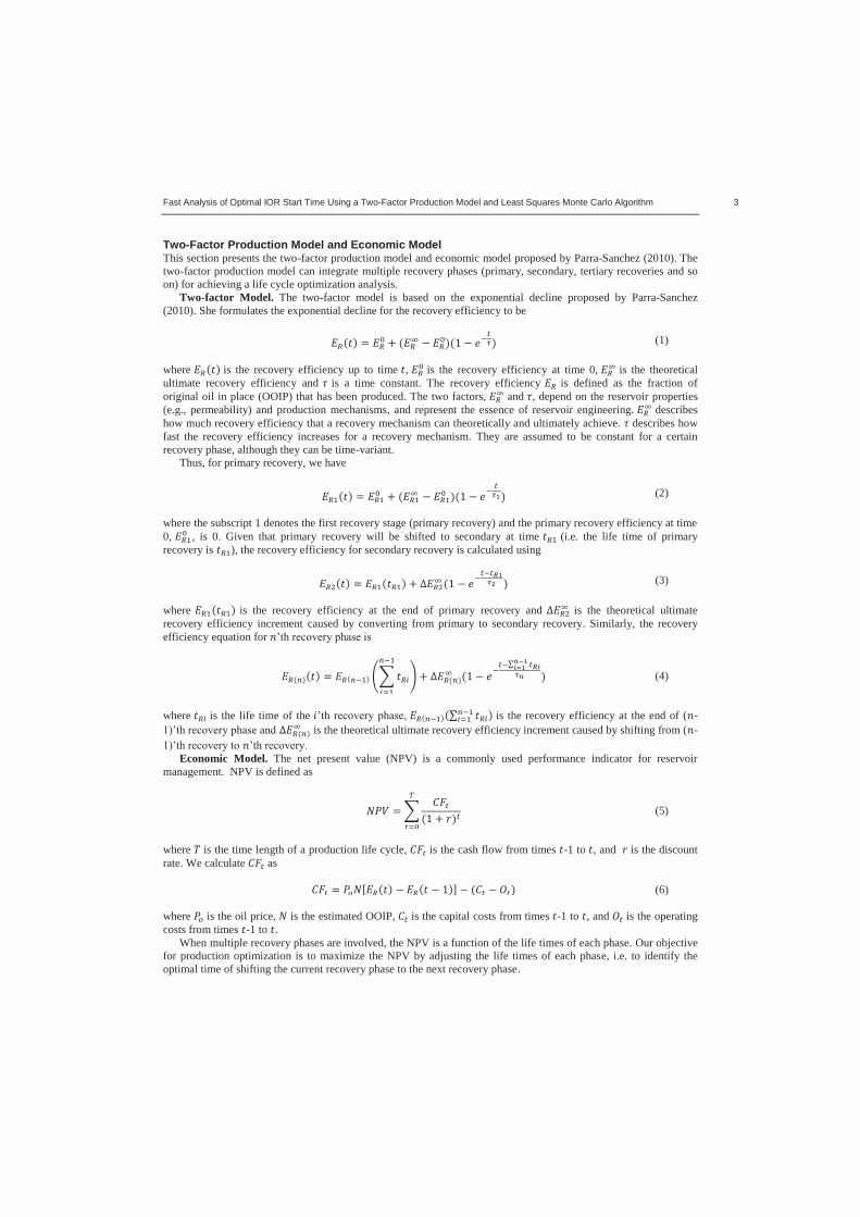
Fast Analysis of Optimal IOR Start Time Using a Two-Factor Production Model and Least Squares Monte Carlo Algorithm 3
Two-Factor Production Model and Economic Model This section presents the two-factor production model and economic model proposed by Parra-Sanchez (2010). The two-factor production model can integrate multiple recovery phases (primary, secondary, tertiary recoveries and so on) for achieving a life cycle optimization analysis.
Two-factor Model. The two-factor model is based on the exponential decline proposed by Parra-Sanchez (2010). She formulates the exponential decline for the recovery efficiency to be
(1) where is the recovery efficiency up to time , is the recovery efficiency at time 0, is the theoretical ultimate recovery efficiency and is a time constant. The recovery efficiency is defined as the fraction of original oil in place (OOIP) that has been produced. The two factors, and , depend on the reservoir properties (e.g., permeability) and production mechanisms, and represent the essence of reservoir engineering. describes how much recovery efficiency that a recovery mechanism can theoretically and ultimately achieve. describes how fast the recovery efficiency increases for a recovery mechanism. They are assumed to be constant for a certain recovery phase, although they can be time-variant.
Thus, for primary recovery, we have
(2)
where the subscript 1 denotes the first recovery stage (primary recovery) and the primary recovery efficiency at time 0, , is 0. Given that primary recovery will be shifted to secondary at time (i.e. the life time of primary recovery is ), the recovery efficiency for secondary recovery is calculated using (3) where is the recovery efficiency at the end of primary recovery and is the theoretical ultimate recovery efficiency increment caused by converting from primary to secondary recovery. Similarly, the recovery efficiency equation for
(4)
where is the life time of the is the recovery efficiency at the end of ( -
is the theoretical ultimate recovery efficiency increment caused by shifting from ( -
Economic Model. The net present value (NPV) is a commonly used performance indicator for reservoir management. NPV is defined as
(5)
where is the time length of a production life cycle, is the cash flow from times -1 to , and is the discount rate. We calculate as (6) where is the oil price, is the estimated OOIP, is the capital costs from times -1 to , and is the operating costs from times -1 to .
When multiple recovery phases are involved, the NPV is a function of the life times of each phase. Our objective for production optimization is to maximize the NPV by adjusting the life times of each phase, i.e. to identify the optimal time of shifting the current recovery phase to the next recovery phase.

Fast Analysis of Optimal IOR Start Time Using a Two-Factor Production Model and Least Squares Monte Carlo Algorithm 4
This work focuses on only geological uncertainties. Thus, the economic model parameters , , and are assumed to be certain values. Refer to Thomas and Bratvold (2015) for the implementation of the LSM algorithm with regards to oil and gas price uncertainties for a gas cap blowdown problem. The uncertainty in the reservoir properties is represented by assigning a probability distribution to each of the model parameters , , and
. For a risk-neutral decision maker2, the objective is to optimize the expected NPV (ENPV) over the uncertain model parameters. Integrating the Impact of Information in Production Optimization In decision making, the optimization problem on deciding the life times of each recovery phase can be interpreted as: for a series of decision points in time; we must decide whether we should continue with the current recovery phase or shift to the next recovery phase at each decision point. This is a sequential decision-making problem. As production continues, we are continuously getting more information from, for example, production data. These data are used to inform our uncertainty in the reservoir properties through history matching, and support our decision making. Thus, in production optimization, we should include the impact of information. A state-of-the-art approach of integrating information in production optimization is the closed loop reservoir management (CLRM) approach. A more advanced approach is the fully structured reservoir management (FSRM) approach. The following briefly presents these two approaches and illustrates the difference between them.
Closed Loop Reservoir Management. ptimization is
closed by continuously update a production model with several realizations and performing life-cycle optimization whenever new data becomes available (Brouwer et al. 2004; Nævdal et al. 2006; Chen et al. 2009; et al. 2009; Jansen et al. 2009).
Several realizations of an initial production model are built based on the prior knowledge of the reservoir, and an initial production strategy for the whole life cycle is determined by optimizing the expected value (EV) over the initial realizations of the production model. The initial production strategy is applied to the real field until new data becomes available. The new data is used to update the production model, and a new production strategy for the period from the time after the new data has become available to the end time of the life cycle is determined by optimizing the EV over the updated realizations of the production model. The new production strategy is applied to the real field until new data becomes available. Repeating the process keeps the reservoir management up to date.
In the viewpoint of sequential decision making, the CLRM is a myopic decision policy where the uncertainties associated with current available data are considered but the uncertainties associated with future data are not (Kullawan 2016; Thomas 2016). A decision tree3 representation for this approach is illustrated in Fig. 1 where denotes a decision made at time and denotes the uncertainties associated with current available data until .
is commonly represented by a production model with several realizations. The production strategy , is determined with the consideration of only the immediate relevant uncertainty .
Fig. 1 Illustration of the decision tree for the CLRM.
The advantage of CLRM is that it greatly simplifies the structure of a reservoir management decision problem
and consequently, requires less computational cost for solving the problem. Its significant drawback is that it does not reflect the full structure of a reservoir management decision problem and thus, may lead to a sub-optimal production strategy.
Fully Structured Reservoir Management. The full structure of a sequential decision-making problem is illustrated by the decision tree in Fig. 2. The FSRM approach aims to solve for the optimal decision policy based on a fully structure decision tree. 2 Risk-neutrality is a risk attitude of being neither risk-averse nor risk-seeking. A risk-neutral decision maker uses only expected value as his decision criterion, i.e., he is indifferent between choices with equal expected values no matter what the risk of a choice is. 3 In a decision tree, a square represents a decision node and a circle represents an uncertainty node.

Fast Analysis of Optimal IOR Start Time Using a Two-Factor Production Model and Least Squares Monte Carlo Algorithm 5
The FSRM explicitly considers both the uncertainties associated with currently available data ( ) and that with future data ( ). Therefore, the current decision ( ) does not depend on only the uncertainties that a decision maker have learnt so far but also the uncertainties that the decision maker will learn in the future. The FSRM includes the dec ) to the uncertainties associated with future data ( ).
Fig. 2 Illustration of the decision tree for FSRM.
Solving the decision tree in Fig. 2 gives the optimal production strategy. However, the FSRM can be
computationally intensive or even prohibitive compared to the CLRM. Least-Squares Monte Carlo Algorithm for Fully Structured Reservoir Management The Least-Squares Monte Carlo (LSM) is a promising algorithm for solving a FSRM problem. It was proposed by Longstaff and Schwartz (2001) for an American option problem which involves a yes-no decision: at anytime, an option holder can decide whether to immediately exercise the option at current stock price or to continue the option for exercising it at future stock price. The stock price is an uncertain quantity in an American option problem, whose uncertainty can be modeled as a Markov process, and thus, the future value of an alternative conditions only to the current stock price.
However, geological uncertainty does not only depend on the currently measured data but also the previously measured data and consequently, the future value of an alternative conditions to currently and previously measured data. To deal with our problem at hand, we slightly modify the LSM algorithm to include the dependency of the future value on the currently and previously measured data. The two central steps of our modified LSM algorithm are
1) Monte Carlo Simulation (MCS) Step: independent samples of model parameters representing geological uncertainties are generated using
MCS. For one sample of model parameters, forward modeling is performed to provide modeled production data from (time 0) to (end time); and then, random noises generated based on the statistics of the measurement errors4 are added to the modeled production data to provide a sample of measured data. Because this sample of measured data consists of a series of data points in time, it is also called a path of measured data. Repeating this procedure for each of the sampled sets of model parameters, we obtain paths of measured data, i.e. .
2) Least Squares Step: For the th sample of model parameters, the NPV of alternative is calculated, giving . This is repeated for the sampled sets of model parameters, resulting in
. To estimate the ENPV with alternative conditional on the measured data, , we regress on . This procedure is repeated for each of the alternatives.
More detailed steps of applying the LSM algorithm will be illustrated in the following example. Illustrative Example This section uses a simple example to illustrate the fully structured decision tree for the problem of determine the optimal IOR start time, the difference between CLRM and FSRM solutions and how to use the LSM algorithm to solve the problem.
Problem Setting. A field has a life cycle of 15 years. We consider a yes-no decision at Years 0, 5 and 10: whether primary recovery should be shifted to secondary recovery. The shift can only happen once. The production is modeled by a function with parameters . The geological uncertainty is represented by 3 realizations (R1, R2 4 In the context of history matching, a common practice is to treat the data fluctuations caused by changes in operating conditions as caused by measurement errors (Jochen and Spivey 1996).

Fast Analysis of Optimal IOR Start Time Using a Two-Factor Production Model and Least Squares Monte Carlo Algorithm 6
and R3) of the production model parameters ( , and ). These realizations are a priori equi-probable. Fig. 3 illustrates the primary recovery efficiency as a function of time for the realizations.
Fig. 3 Primary recovery as a function of time for 3 geological realizations.
The NPVs corresponding to each alternative and each realization are in Table 1. All the values are in million
USD.
Realization Shift at Time No Shift R1 1700 1880 2170 3500 R2 1800 2240 2430 2130 R3 2430 3540 3110 1810
Table 1 NPVs corresponds to each alternative and each realization.
The measured primary recovery efficiency is used to inform the decisions. The likelihood functions, listed in
Table 2, are used to describe the measurement errors. For example, given that the truth is R1, the probability of the measurement at measured data of 0.18) is 0.75, and the probability of the measurement at
Given the truth is R1 R2 R3
Measurement at says
0.75 0.25 0.75
0.25 0.75 0.25
Measurement at says
0.80 0.20 0.20
0.20 0.80 0.80
Table 2 Likelihood functions for the measured primary recovery efficiency.
Decision and Expected Value without Information. If the impact of future information on the series of
decisions is not considered, the ENPV is calculated based on the a priori probability of each realization (i.e. 1/3). For this case, the optimal decision is referred to as the decision without information (DWOI), and the corresponding optimal EV is referred to as the EV without information (EVWOI). Thus, the DWOI is EVWOI of $2570 million.
Decision and Expected Value with Perfect Information. Perfect information reveals the truth. For example, if the perfect information indicates R1, then R1 is the truth and we can identify the optimal decision by maximizing the NPV of R1. The optimal decision and EV for this case are referred to as the decision and EV with perfect information (DWPI and EVWPI), respectively. time

Fast Analysis of Optimal IOR Start Time Using a Two-Factor Production Model and Least Squares Monte Carlo Algorithm 7
EVWPI of $3156.7 million. The value-of-perfect-information (VOPI)5 is thus EVWPI EVWOI = $3156.7 million $2570.0 million = $586.7 million.
FSRM Solution: Decision and Expected Value with Imperfect Information. The likelihood functions in Table 2 indicate the reliability of the data and show that the information is imperfect. The optimal decision and EV for such case are referred to as the decision and EV with imperfect information (DWII and EVWII), respectively.
We construct the full decision three for this problem setting, as illustrated in Fig. 4, to help in identifying the DWII and EVWII. From the tree, we can see that we should continue with primary recovery at no matter what the measurement at says, and continue with primary recovery at if the measurement at recovery at if the measurement at The corresponding EVWII is $2818 million, resulting in a value-of-information (VOI) of EVWII EVWOI = $2818 million $2570 million = $248 million.
CLRM Solution. We solve the same problem using the CLRM approach. Unlike that the FSRM approach which solves the decision tree backwards (i.e. rollback from the right nodes to the left-most node in the tree), the CLRM approach solves the tree forwards. For example, given the measurement at probabilities of R1, R2 and R3 are 0.43, 0.14 and 0.43, respectively; based on these probabilities, the EV is $2642.9 million for ing at no shift
is to shift to secondary recovery. The decision policy of the CLRM approach is listed in Table 3. Applying this decision policy to the decision tree in Fig. 2 results in an EV of $2641.2 million corresponding to a special VOI6 of $71.2 million.
Compared to the FSRM approach, the CLRM approach gives a difference decision policy and a lower VOI. The CLRM approach realizes only 71.2/248 = 28.7% of the value that the information can create. This is because when the impact of future information is not considered in the CLRM approach, the CLRM approach makes a decision based on the immediate gain rather than evaluating whether it is worth continuing for gathering more information as the FSRM approach does.
Decision at Time
Continue with primary recovery.
Shift to secondary recovery if measurement at
No action because it has been shifted to secondary recovery at .
Continue with primary recovery if the measurement at says
Continue with primary recovery if the measurement at
Shift to secondary recovery
if the measurement at
Table 3 Decision policy of the CLRM approach.
5 The concept of value-of-information (VOI) originates from the decision analysis community. VOI is an indicator of the maximal paying price or cost of an information gathering activity. VOPI is the upper limit of VOI. For a more comprehensive description of the concept of VOI, consult Raiffa and Schlaifer (1961), Howard (1966), and Bratvold et al. (2009). For the illustration and discussion of adopting the concept of VOI in history matching contexts, refer to Hong and Bratvold (2017). 6 Per the strict definition of VOI, it is referred exclusively to that associated with the optimal decision policy (i.e. the
sub-optimal decision policy (i.e. the CLRM approach in our case).

Fast Analysis of Optimal IOR Start Time Using a Two-Factor Production Model and Least Squares Monte Carlo Algorithm 8
Fig. 4 Fully structured decision tree for the illustrative example.
Solving the FSRM Problem Using the LSM Algorithm. We use the modified LSM algorithm to solve the
FSRM problem as shown in Fig. 4. For illustration, we use only 6 Monte Carlo samples. The number of samples will be increased later to verify the modified LSM algorithm. We first sample 6 paths of the measured data as listed in Table 4. Then, we start the LSM from the last decision point as we solve the decision tree backwards. Table 5
(to secondary for each path.
Path Geological Realization
Data at ( ) ( )
1 R2 0.18 0.22 2 R1 0.18 0.34 3 R3 0.13 0.34 4 R1 0.13 0.34 5 R3 0.18 0.22 6 R2 0.13 0.22
Table 4 Path of measured data for LSM.

Fast Analysis of Optimal IOR Start Time Using a Two-Factor Production Model and Least Squares Monte Carlo Algorithm 9
Path Geological Realization
NPV [million USD] Continue Shift
1 R2 2130.0 2430.0 2 R1 3500.0 2170.0 3 R3 1810.0 3110.0 4 R1 3500.0 2170.0 5 R3 1810.0 3110.0 6 R2 2130.0 2430.0
Table 5 NPVs for alternatives at time for LSM.
When we are making the decision at , we have obtained the data at both and . Therefore, the ENPV is
conditional on the data at both and . We estimate the ENPV by regressing NPV on data. Using ,
. The same is d Table 6 lists for each path. Now, we can make
the optimal decision by taking the alternative that gives the highest ENPV for each path. The optimal decision is colored in red in Table 6.
Path ENPV [million USD] Continue Shift
1 2137.5 2635.0 2 3165.0 2440.0 3 2822.5 2505.0 4 2822.5 2505.0 5 2137.5 2635.0 6 1795.0 2700.0
Table 6 ENPVs for alternatives at time for LSM.
We move one time step backwards to . Table 7
5 for the optimal decisions shown in Table 6.
Path Geological Realization
NPV [million USD] Continue Shift
1 R2 2430.0 2240.0 2 R1 3500.0 1880.0 3 R3 1810.0 3540.0 4 R1 3500.0 1880.0 5 R3 3110.0 3540.0 6 R2 2430.0 2240.0
Table 7 NPVs for alternatives at time for LSM.
When we are making the decision at , the data at only is available but not . Therefore, the ENPV is
conditional on the data at only . Using , the resulting conditional expectation Table
8 for each path, and the optimal decisions are in red.

Fast Analysis of Optimal IOR Start Time Using a Two-Factor Production Model and Least Squares Monte Carlo Algorithm 10
Path ENPV [million USD] Continue Shift
1 3013.3 2553.3 2 3013.3 2553.3 3 2580.0 2553.3 4 2580.0 2553.3 5 3013.3 2553.3 6 2580.0 2553.3
Table 8 ENPVs for alternatives at time for LSM.
We move to . Table 9 for each
imal decisions shown in Table 8. Because we have no data available at , we calculatmean of the values in columns 4 and 5, respectively, in Table 2796.7
1976.7 million. Thus, the optimal decision at is $2796.7 million.
Path Geological Realization
NPV [million USD] Continue Shift
1 R2 2430.0 1800.0 2 R1 3500.0 1700.0 3 R3 1810.0 2430.0 4 R1 3500.0 1700.0 5 R3 3110.0 2430.0 6 R2 2430.0 1800.0
Table 9 NPVs for alternatives at time for LSM.
The optimal decision policy can be determined by looking back at Table 8 and Table 6, and it is represented by
Table 10.
Path Data at Optimal Decision at ( ) ( )
1 0.18 0.22 Continue Continue Shift 2 0.18 0.34 Continue Continue Continue 3 0.13 0.34 Continue Continue Continue 4 0.13 0.34 Continue Continue Continue 5 0.18 0.22 Continue Continue Shift 6 0.13 0.22 Continue Continue Shift
Table 10 Table representation of optimal decision policy solved using LSM.
The optimal ENPV and optimal decision policy solved using the modified LSM are different from the analytical
solution from the decision tree (Fig. 4) because we used only 6 paths. The accuracy can be improved by increasing the number of paths. We increase to 500000 paths and repeat it for 1000 times. This gives a mean of estimated optimal ENPV of $2818.03 million, which is almost the same as the analytical solution $2818.00 million, and a standard deviation of $0.80 million (which is relatively small). This verifies the accuracy of using the modified LSM algorithm to solve the FSRM problem.
Application of the Two-Factor Production Model and the Least Squares Monte Carlo Algorithm This section uses a more realistic example to illustrate the application of the two-factor production model and the LSM algorithm for analyzing the optimal IOR start time. This example is more complicate than the illustrative

Fast Analysis of Optimal IOR Start Time Using a Two-Factor Production Model and Least Squares Monte Carlo Algorithm 11
example. Thus, a fully structured decision tree cannot be visualized and the problem cannot be solved by simply rollback a decision tree. The modified LSM algorithm is therefore of significant use for this example.
Problem Setting. In the development phase of an oil field, we consider two recovery phases primary and secondary recovery. We want to analyze the optimal time of shifting from the primary recovery to the secondary recovery and the optimal time of terminating the production (i.e. to identify the optimal life times of primary and secondary recoveries). This analysis provides useful insights in how the field should be developed and how the leaning over time will impact the decisions. We consider a maximal life cycle of 50 years. The shift can happen at the beginning of any year but only once, and the same for the termination. In other words, we need to decide whether to continue with the primary recovery, to shift to the secondary recovery, or to terminate the production at the beginning of each year from Year 1 to Year 50.
The oil production is modeled using the two-factor production model. We assign probability distributions to the model parameters based on a priori knowledge to represent the uncertainties in reservoir properties and the effects of the primary and secondary recovery mechanism. All the parameters are assumed to be normally distributed and their means and standard deviations are in Table 11. The correlation coefficient between the parameters are in Table 12.
Parameter [fraction] [years] [fraction] [years]
Mean 0.20 16 0.15 7 Standard Deviation 0.05 2 0.05 1.5
Table 11 Means and standard deviations for the normal distributions of the production model parameters.
1 0.2 -0.7 0.1
0.2 1 -0.3 -0.2 -0.7 -0.3 1 -0.3
0.1 -0.2 -0.3 1 Table 12 Correlation coefficients between the production model parameters.
Because we focus on the geological uncertainty, we assume all the parameters of the economic model are known
and their values are in Table 13. The capital cost is paid at the beginning of each recovery phase. The cashflow is discounted yearly.
Parameter Value Unit
OOIP 240 million bbl Oil Price 55 USD/bbl
Capital Cost (Primary) 50 million USD Capital Cost (Secondary) 50 million USD Operating Cost (Primary) 9.1 million USD/year
Operating Cost (Secondary) 21.1 million USD/year Discount Rate 12% yearly
Table 13 Values of economic parameters.
The recovery efficiency is measured at the end of each year and is used to support the decisions. The
measurement error is assumed to be normally distributed with zero mean and a standard deviation of 0.001. Results. secondary recovery, leading to a life
cycle of 24 years. The corresponding EVWOI is $918.9 million. If we can obtain perfect information on the reservoir properties and the effects of primary and secondary recovery mechanisms before the production starts, the resulting EVWPI is $1057.6 million. Thus, the VOPI is $138.7 million. This value indicates that the total costs of any additional data gathering activity (e.g., conducting a seismic survey), no matter how sophisticated it is, for better understanding the reservoir properties or the effects of primary and secondary recovery mechanisms should not exceed $138.7 million. The FSRM approach leads to an EVWII of $991.8 million for the measure of recovery efficiency. The corresponding VOI is $72.9 million. Therefore, the company should not pay more than $72.9 million to buy and install devices for measuring the recovery efficiency.

Fast Analysis of Optimal IOR Start Time Using a Two-Factor Production Model and Least Squares Monte Carlo Algorithm 12
Fig. 14 compares the cumulative density functions (CDFs) of NPVs corresponding to the DWOI, DWII and DWPI. We see that the FSRM approach moves the CDF of NPVs corresponding to the DWOI to the right (i.e. the NPV increases) because it allows for learning over time. We notice that some realizations (around 5%) end up with a smaller NPV with DWII than the NPV with DWOI. The possible reasons are: (1) the downside (e.g., the theoretical ultimate recovery efficiency increment turns out to be very small) may show up even though the decision
future events, and/or (2) a sub-optimal decision may be made because the LSM algorithm is an approximation method. The DWPI further moves the CDF curve to the right, leading to a higher ENPV than that of the DWOI and DWII.
Fig. 14 CDFs of NPVs corresponding to DWOI, DWII and DWPI.
The probability density functions (PDFs) and CDFs of the primary recovery, secondary recovery and total life
times corresponding to the DWII are in Figs. 15 17 where the DWOI is marked in red. Fig. 15 shows that the P10 P90 interval of the primary recovery life time ranges from 1 to 20 years (i.e. there is
80% chance that the recovery mechanism should be shifted from primary to secondary anytime from Year 1 to Year 20). This is a wide range. The specific timing of shifting depends on the measure of recovery efficiency. There is only 4% chance that it is optimal to
y of more than 20%. This informs that the facilities for the
company will lose the flexibility , which has a chance of about 35% to happen.
Fig. 16 shows that the P10 P90 interval of the secondary recovery life time ranges from 12 to 22 years. The 18 to happen while the most probable (13%)
secondary recovery life time is 19 years. Besides, there is 40% chance that the secondary recovery life time is shorter than 18 years and 48.5% chance longer.
Fig. 17 shows that the P10 P90 interval of the total life time ranges from 19 to 36 years. This informs that it would better to has a license for production up to 36 years and a flexibility to terminate the production or sell their contract any time from Year 19 to Year 36. If the license for production lasts only 24 years according to the DWOI, the company would have a chance of more than 60% to lose the opportunity of producing longer.

Fast Analysis of Optimal IOR Start Time Using a Two-Factor Production Model and Least Squares Monte Carlo Algorithm 13
Fig. 15 PDF and CDF of the primary recovery lifetime corresponding to the DWII.
Fig. 16 PDF and CDF of the secondary recovery lifetime corresponding to the DWII.
Fig. 17 PDF and CDF of the total lifetime corresponding to the DWII.
Fig. 18 illustrates the probabilities for different combinations of primary and secondary recovery life times
corresponding to the DWII. The more probable combinations are primary recovery lifetime for 1 year combined with secondary recovery life time for 17 to 23 years. These combinations have a probability more than twice than the other combinations. This may because we assigned 16 years to the mean value of and 7 years to the mean value of , which means that the secondary recovery mechanism will recovery oil faster than the primary recovery mechanism. Per the NPV calculation, the higher the cash flow is at the early times, the higher the NPV is. Shifting primary recovery to secondary recovery at an early time will results in a higher NPV than doing that at a later time.
The highly probable (>0.5%) combinations can be separated into two groups: (1) small span of primary recovery life time (1 2 years) with large span of secondary recovery life time (13 24 years), and (2) small span of secondary recovery life time (17 21 years) with large span of primary recover life time (5 17 years). The correlation

Fast Analysis of Optimal IOR Start Time Using a Two-Factor Production Model and Least Squares Monte Carlo Algorithm 14
coefficient between the primary and secondary recovery life time is -0.44. This negative linear correlation is because there is a strong negative linear correlation between the theoretical ultimate primary recovery efficiency and the theoretical ultimate recovery efficiency increment as assigned in Table 12.7 That is, if the primary recovery can already lead to a relatively high ultimate recovery efficiency, then the recovery efficiency increment of the secondary recovery will be relatively low (i.e. more effective the primary recovery is, less effective the secondary recovery is). Consequently, we can expect a relatively short secondary recovery life time if the data inform us to continue with primary recovery for a relatively long time.
Fig. 18 Probabilities for different combinations of primary and secondary recovery life times.
Discussion The two-factor production model is useful and tractable. When it is combined with the LSM algorithm, a fast analysis of optimal IOR start time and life time can be realized with the consideration of the impact of future information. Although the model is very simple, the analysis provides many useful insights in the decision problem. The FSRM solution contains a decision policy, reaction to information, rather than a single value of the decision variable. The solutions of this fast analysis can then be interrogated with sophisticated simulations if adding details in the production model is deemed to be relevant and material for the decisions at hand.
The LSM algorithm is an approximate dynamic programming method. Its accuracy depends on two factors: the number of Monte Carlo samples and how well the regression function approximates the real EV. Because we used very many Monte Carlo samples (500000), we believe that the sampling error is negligible. We used a first order linear regression function, the simplest form of a regression function. The illustrative example tested this regression function and showed that it provided high accuracy. It seems from the results that this regression function performed well for the more complex application of the LSM algorithm. Although a more complicated regression function (for example, with higher order) can improve the accuracy, we think the simple fist order linear regression function is sufficient to extract high quality insight for our problem setting.
This work focused only on the geological uncertainty represented by the two-factor model parameters. However, the uncertainty in economic model parameters can be included by adding these variables into the regression function. It is easier to handle the economic variables than the production data. The economic variables are usually assumed to follow a Markov chain. Thus, the EV is conditional on only their most recent value unlike that the EV, which is conditional on the full path of the production data.
We considered only two recovery phases the primary and secondary recovery phases. More recovery phases should be included for a more comprehensive analysis of the production life cycle. The inclusion of more recovery phases (i.e. introducing more alternatives at each decision point) will require more computational time for the LSM algorithm. Generally, the computational time increases exponentially with the number of alternatives. Thus, 7 We assign a negative linear correlation between the theoretical ultimate primary recovery efficiency and the theoretical ultimate recovery efficiency increment for illustrative purpose only. The correlation can be any value from -1 to 1, depending on reservoir properties, well locations, recovery mechanisms, production strategies, etc.

Fast Analysis of Optimal IOR Start Time Using a Two-Factor Production Model and Least Squares Monte Carlo Algorithm 15
including too many recovery phases may become computationally prohibitive even when a computationally attractive production model is used. Conclusions This paper reviewed a useful and tractable model for modeling various recovery phases involved in a life cycle of oil production and illustrated the detailed steps of implementing the LSM algorithm to solve a sequential decision-making problem.
We demonstrated the value of considering the impact of future information in the analysis of the optimal IOR start time. We used an illustrative example to discuss the full structure of the relevant decision problem. Although the state-of-the-art reservoir management approach CLRM can lead to larger EV than the case without considering the impact of information, its solution may be sub-optimal. It is because it considers only the information obtained before a decision is made but not the information obtained after that decision. The optimal solution can be guaranteed using the FSRM approach.
A more realistic example demonstrated the application of the two-factor model and the LSM algorithm. The results showed that the FSRM approach can significantly improve the decisions and leads to a significant increase in ENPV. The resulting decision policy represents the optimal action a decision maker should take according to his/her observation.
We conclude that using the two-factor model and the LSM algorithm can, with limited computation resources, provide useful insights in the problem of deciding the optimal IOR start time.
Acknowledgements The authors acknowledge the support of the Research Council of Norway and industry partners: ConocoPhillips, Skandinavia AS, BP Norge AS, Det Norske Oljeselskap AS, Eni Norge AS, Maersk Oil Norway AS, DONG Energy A/S, Denmark, Statoil Petroleum AS, ENGIE E&P NORGE AS, Lundin Norway AS, Halliburton AS, Schlumberger Norge AS, and Wintershall Norge AS of The National IOR Centre of Norway.
Aojie Hong would like to thank the staffs and colleagues at the University of Texas at Austin for their support during his visiting. Larry W. Lake holds the Shahid and Sharon Ullah Chair at the University of Texas. References Alkhatib, A. M., and King, P. R. 2011. Applying Real Options Theory in Determining Optimal Policies for a
Surfactant Flood. Presented at the SPE Enhanced Oil Recovery Conference, Kuala Lumpur, Malaysia, 1921 July. SPE-144869-MS. http://dx.doi.org/10.2118/144869-MS.
Bickel, J. E., and Bratvold, R. B. 2008. From Uncertainty Quantification to Decision Making in the Oil and Gas Industry. Energy Exploration & Exploitation 26 (5): 311 325. https://doi.org/10.1260/014459808787945344.
Bratvold, R. B., and Begg, S. 2010. Making Good Decisions, first edition. Texas, USA: Society of Petroleum Engineers.
Bratvold, R. B., Bickel, J. E., and Lohne, H. P. 2009. Value of Information in the Oil and Gas Industry: Past, Present, and Future. SPE Reservoir Evaluation & Engineering 12 (4): 630 638. SPE-110378-PA. http://dx.doi.org/10.2118/110378-PA.
Brouwer, D. R., Nævdal, G., Jansen, J. D. et al. 2004. Improved Reservoir Management Through Optimal Control and Continuous Model Updating. Presented at the SPE Annual Technical Conference and Exhibition, Houston, USA, 26 29 September. SPE-90149-MS. https://doi.org/10.2118/90149-MS.
Chen, Y., Oliver, D. S., Zhang, D. 2009. Efficient Ensemble-Based Closed-Loop Production Optimization. SPE Journal 14 (4): 634 645. SPE-112873-PA. https://doi.org/10.2118/112873-PA.
Howard, R. A. 1966. Information Value Theory. IEEE Transactions on Systems Science and Cybernetics 2 (1): 2226. http://dx.doi.org/10.1109/TSSC.1966.300074.
Howard, R. A., and Abbas, A. E. 2016. Foundations of Decision Analysis, global edition. Harlow, England: Pearson Education Limited.
Hong, A. J., and Bratvold, R. B. 2017. Value of Information from History Matching How Much Information is Enough? Presented at the IOR NORWAY 2017 19th European Symposium on Improved Oil Recovery, Stavanger, Norway, 24 27 April. https://doi.org/10.3997/2214-4609.201700327.
Hong, A. J., Bratvold, R. B., and Nævdal, G. 2017. Robust Production Optimization with Capacitance-Resistance Model as Precursor. Computational Geosciences. https://doi.org/10.1007/s10596-017-9666-8.
Hem, Ø. D., Svendsen, A., Fleten, S. E. et al. 2011. The Option to Switch from Oil to Natural Gas in Active Offshore Petroleum Fields. Presented at the Annual International Real Options Conference, Turku, Finland,

Fast Analysis of Optimal IOR Start Time Using a Two-Factor Production Model and Least Squares Monte Carlo Algorithm 16
15 18 June. Jafarizadeh, B., and Bratvold, R. B. 2012. Two-Factor Oil-Price Model and Real Option Valuation: an Example of
Oilfield Abandonment. SPE Economics & Management 4 (3): 158 170. SPE-162862-PA. http://dx.doi.org/10.2118/162862-PA.
Jafarizadeh, B., and Bratvold, R. B. 2013. Sell Spot or Sell Forward? Analysis of Oil-Trading Decisions with the Two-Factor Price Model and Simulation. SPE Economics & Management 5 (3): 80 88. SPE-165581-PA. http://dx.doi.org/10.2118/165581-PA.
Jansen, J. D., Brouwer, R., Douma, S. G. 2009. Closed Loop Reservoir Management. Presented at the SPE Reservoir Simulation Symposium, The Woodlands, USA, 2 4 February. SPE-119098-MS. https://doi.org/10.2118/119098-MS.
Jochen, V. A., and Spivey, J. P. 1996. Probabilistic Reserves Estimation Using Decline Curve Analysis with the Bootstrap Method. Presented at the SPE Annual Technical Conference and Exhibition, Denver, USA, 6 9 October. SPE-36633-MS. http://dx.doi.org/10.2118/36633-MS.
Kullawan, K. 2016. A Bayesian Framework for Real-Time Optimization of Well Placement. PhD Thesis. The University of Stavanger, Norway.
Longstaff, F., and Schwartz, E. 2001. Valuing American Options by Simulation: a Simple Least-Squares Approach. Review of Financial Studies 14 (1): 113 147. http://dx.doi.org/10.1093/rfs/14.1.113.
Nævdal, G., Brouwer, D. R., Jansen, J. D. 2006. Waterflooding Using Closed-Loop Control. Computational Geosciences 10 (1): 37 60. https://doi.org/10.1007/s10596-005-9010-6.
Raiffa, H., and Schlaifer, R. 1961. Applied Statistical Decision Theory. Boston: Division of Research, Graduate School of Business Administration, Harvard University (Reprint).
Parra-Sanchez, C. 2010. A Life Cycle Optimization Approach to Hydrocarbon Recovery. Master Thesis. The University of Texas at Austin, USA.
Thomas, P. 2016. Managing Uncertainty with Decision Analysis in The Oil and Gas Industry. PhD Thesis. The University of Stavanger, Norway.
Thomas, P, and Bratvold, R. B. 2015. A Real Options Approach to the Gas Cap Blowdown Decision. Presented at the SPE Annual Technical Conference and Exhibition, Houston, USA, 28 30 September. SPE-174868-MS. https://doi.org/10.2118/174868-MS.
Willigers, B. J. A., Begg, S. H., and Bratvold, R. B. 2011. Valuation of Swing Contracts by Least-Squares Monte Carlo Simulation. SPE Economics & Management 3 (4): 215 225. SPE-133044-PA. http://dx.doi.org/10.2118/133044-PA.
Wang, C., Li, G., Reynolds, A. C. 2009. Production Optimization in Closed-Loop Reservoir Management. SPE journal 14 (3): 506 523. SPE-109805-PA. https://doi.org/10.2118/109805-PA.

Paper IV
Robust Discretization of Continuous Probability Distributions for Value-of-
Information Analysis Bratvold, R.B., Thomas, P., Begg, S.H., and Hong, A.J.


Figure 1 - Discrete PMF approximation (blue) to the continuous (red) PDF.


Figure 2 - Decision tree for valuing information for the case with three alternatives and three discrete outcomes.


Figure 3 - EVII as a function of correlation between the prior and the observed signal.
Table 1 - Discretization shortcuts

Figure 4 - Comparison of approximate EVII to exact EVII for commonly used discretization methods.
Discussion
reliability
o
o
oo
o

o
Deriving the Signal or Likelihood Distributions
Discretization

General Methods for Discretizing the Likelihood
Likelihood derived through the correlation coefficient

General likelihood for any functional form
Validation of the HRPT approach

Figure 5 - Likelihood, Joint and Posterior probability density functions for different correlation coefficients between the uncertain quantity of interest, , and the signal, .

Figure 6 - Comparison of approximate EVII to exact EVII for different values of .
Table 2 – Percent error when using the HRPT approach in a TALL-N, problem for different and .

Figure 7 - Comparison of approximate EVII to exact EVII for different value of N when the information gathering cost is included.
PERT – PERT prior – likelihood pair

Figure 8 - VoI from HRPT vs cost of information gathering – PERT – PERT prior – likelihood pair.
Lognormal – lognormal prior – likelihood pair
Figure 9 - VoI from HRPT vs cost of information gathering – lognormal – lognormal prior – likelihood pair.
Moment Matching

Bracket Mean and Bracket median
Table 3- PERT prior and lognormal prior discretization methods

Figure 10 - VoI error for the general discretization methods with PERT Prior, 5 points discretization Figure 11 - VoI error for the general discretization methods
with lognormal Prior, 5 points discretization
Figure 12 - VoI error for the general discretization methods with PERT Prior, 3 points discretization
Figure 13 - VoI error for the general discretization methods with lognormal prior, 3 points discretization

Figure 14 - VoI error for the discretization shortcuts with PERT prior
Figure 15 - VoI error for the discretization shortcuts with lognormal prior
Figure 16 - Range of relative errors using the PERT prior Figure 17 - Range of relative errors using the lognormal
prior

Figure 18 - Effect of VoI error on the information gathering decision
n k

Bayes Monte Carlo (BMC).
Figure 19 - Illustration of HRPT discretized outcomes and Monte Carlo samples for a continuous probability distribution.
Ensemble Kalman Filter (EnKF).

Comparison to HRPT and Analytical VoI.
Figure 20 - VoI Mean Squared Error of VoI for HRPT and EnKF

Figure 21 - Linear loss integral of NPV distribution for lognormal case.

Computers & Mathematics with Applications.
IFAC-PapersOnLine.
Computational Geosciences.
Introduction to probabilityDecision Analysis.
SPE Economics & Management.
SPE Economics & Management.
Making good decisionsSPE Reservoir
Evaluation & Engineering.Monthly weather review.
Making hard decisions with decision tools
Journal of Geophysical Research: Oceans.
Decision analysis for the professional—with supertree
Decision analysis for petroleum exploration
Applied statistical decision theory
Probability and statistics for business decisions; an introduction to managerial economics under uncertainty

Optimal control and estimationRisk analysis : a quantitative guide
An introduction to Bayesian inference and decision
x x z z
x x z z
x z
x x z z
f x z
Zi i
X
E Z X x E Z x E X
XVAR Z X
m vNmv m
z
z
z
z
N

Ensemble Kalman Filter (EnKF).

K
EnKF formulation to Analytical VoI for TALL-N
z
z x
N N N Nk ij i
i j k kVOI v x z v x
N N N
p
x N
x N z N
K

x
x z x
E x z x z x
xx
x z xx z x
Var x z

Paper V
Value-of-Information for Model Parameter Updating through History Matching
Hong, A.J., Bratvold, R.B., Thomas, P., and Hanea, R.G.


Value-of-Information for Model Parameter Updating through History Matching 1
Manuscript Value-of-Information for Model Parameter Updating through History Matching A.J. Hong and R.B. Bratvold, University of Stavanger and The National IOR Centre of Norway; P. Thomas, University of Stavanger; and R.G. Hanea, University of Stavanger and Statoil ASA
Abstract The oil and gas (O&G) industry spends billions of dollars on data (e.g., production data, seismic data and tracer data) gathering and analysis for the purpose of reducing uncertainty and improving their understanding of the most salient features of the subsurface. Yet, the O&G industry spends minimal effort and investment to assess whether the benefit of this data gathering and analysis exceeds the cost. One form of data gathering and analysis is history matching (HM), which has been an essential reservoir management tool for decades. This paper addresses the value of HM by applying the value-of-information (VOI) framework originally developed in the decision sciences.
There are several challenges involved in assessing the VOI in the HM context. Although reservoir management (HM and production optimization) and decision analysis (DA) use many of the same methods, the two domains involve different terminology used in fluid flow modeling and application of state-of-the-art HM and optimization methods. Furthermore, most applications of VOI analysis have focused on static, as opposed to time-dependent, analysis. Finally, some recent publications in the O&G industry that have illustrated and discussed VOI from HM have not been consistent with the original definition of VOI.
In this paper, we illustrate and discuss the use of a consistent, DA-based, VOI analysis framework to assess the VOI in HM contexts. In order to make the VOI framework understandable and accessible to both the reservoir management and DA communities, we provide a terminology used in VOI calculations and that used in state-of-the-art HM and optimization methods.
The paper includes four VOI analysis examples. The first illustrates the implementation of the general VOI framework for a simple HM problem. The second illustrates and discusses the difference between the calculations presented by other authors and the standard VOI definition used in the DA community. The third illustrates the implementation of VOI calculations in more realistic settings, including a sensitivity analysis of measurement noise. The fourth illustrates the application of VOI assessment in a case where a reservoir simulation model is involved. Introduction Petroleum engineers and geoscientists involved in reservoir management continually e aim of improving decision mak acquisition broadly defined here, to cover such activities as acquiring data, performing technical studies, hiring consultants, and performing diagnostic tests. In fact, other than to meet applicable regulatory requirements, the main reason for collecting any information or doing any technical analysis should be to make better decisions. The fundamental question for any information-gathering process is then whether the likely improvement in decision making is worth the cost of obtaining the information. This is the question that value-of-information (VOI) technique is designed to answer.
VOI analysis is an a priori1 analysis that evaluates the benefits of collecting additional information before one actually gathers the data and makes a decision. Such information gathering might be worthwhile if it could change the decision that would have been made without further information. Although many engineers and geoscientists tend to believe that more information or data is always better, VOI assigns
is added by enabling the decito the underlying uncertainty. Thus, information value is forever an entanglement of uncertainty and decision making; one cannot value information outside of a particular decision context (Bratvold et al. 2009).
1 A priori mean before the data are gathered and interpreted .

Value-of-Information for Model Parameter Updating through History Matching 2
The concept of VOI2 originates from the decision analysis (DA) community. Schlaifer (1959) was the first to define VOI in the context of business decisions. Other early references to VOI analysis can be found in Raiffa and Schlaifer (1961) and Howard (1966). Its use has been documented in wide areas of real-world application, from nuclear waste storage assessment (Eppel and von Winterfeldt 2008) to biosurveillance (Willis and Moore 2013). Grayson (1960) introduced this concept in the oil and gas (O&G) industry. Bratvold et al. (2009) presented the definition of VOI as well as an overview of its use in the O&G industry. Eidsvik et al. (2015) provided a more recent exposition of VOI in the earth sciences.
Although it is more than half a century since the VOI concept was first introduced in the petroleum literature, it has seen limited use in the O&G industry. Most of the published papers that discuss and apply VOI analysis focus on common exploration and development decisions, and most of these applications focus on static, as opposed to time-dependent, analysis. Only recently has the concept been discussed in the context of history matching (HM) which involves data gathered at different times (Barros et al. 2015a, 2015b, 2016a).
HM has been an essential reservoir management tool for decades. Originally, HM referred to the adjustment of the production model parameters to reflect the historical production data (rates and pressures) as closely as possible. Today, the term HM is often used in a broader context and includes model calibration3 using any relevant data and information (seismic data, log data, tracer behavior, etc.). Once the measured data have is used to generate possible future production profiles and their probabilities; i.e., the future production uncertainty, and thus support reservoir management decisions.
With the increase in available computing power over the past several decades, numerical techniques for model-based optimization of subsurface hydrocarbon production have evolved rapidly. The traditional manual approach to HM has in many companies been replaced by automatic or semi-automatic approaches based on robust and efficient numerical algorithms that allow for the inclusion of geological and petrophysical uncertainties. A particularly promising method for HM is the ensemble Kalman filter (EnKF) approach introduced by Evensen (1994). EnKF is based on a Bayesian approach where data is used to quantify geological and petrophysical uncertainties, ensuring consistency in the updated probabilities. The resulting production forecast captures these uncertainties and provides possible production scenarios with associated probabilities; i.e., the uncertain future production.
Although operators in the O&G industry commit significant effort and cost to calibrating their production models, few publications have discussed the a priori value of gathering the data and conducting the calibration. The usefulness of information from HM has been quantified in terms of uncertainty reduction (Le and Reynolds 2014) or by the fraction of information extracted from the measured data (Krymskaya et al. 2010). However, neither concept constitutes an information valuation approach as defined by the DA community, nor is either of them an a priori assessment of the value of the information.
Barros et al. (2015a, 2015b, 2016a) proposed a workflow to assess the VOI in the HM context using ensemble-based4 HM and optimization methods, and later on, Barros et al. (2016b) applied clustering techniques to speed up the previous workflow. Although they have considered the impact of additional information on decision making, the VOI assessed through their workflow is conceptually inconsistent with the definition of VOI as it will be discussed later. Furthermore, they employed terminology and notation that differ significantly from those commonly used in VOI analysis. Indeed, the work by Barros and co-authors is one of the few to claim the use of decision analytic methods to assess VOI in the context of HM. Their workflow mimics in the best possible way the decision process that will happen during reservoir management, but their work is lack of the DA touch and the clarity about why the value they are calculating is VOI. It is important not only to show how the VOI should be assessed but also to illustrate and discuss whether or not their approach is providing the VOI from HM. In this paper, we refer to their workflow (particularly, the workflow introduced in Barros et al. (2015a) s workflow. Since transparency is a key feature of DA community, we try to
, and to s , and then
s workflow. The main contributions of this paper are three-fold. First, we illustrate how VOI analysis can be applied to assess
the information value of gathering production data and performing HM. This requires reconciling the terms used in VOI analysis versus those in state-of-the-art HM methods, especially EnKF for HM.5 Second, we discuss the
2 This paper -of-i as the term is understood in the DA community. 3 . We will use
4 An ensemble means a set of realizations. 5 Some of the terminology used in EnKF also appears in other approaches to HM in the O&G industry.

Value-of-Information for Model Parameter Updating through History Matching 3
differences and similarities between the analysis suggested by Barros et al. (2015a) and VOI analysis. Finally, we present four VOI analysis examples: the first is illustrating the calculation steps of VOI analysis on a simple HM case with the use of decision trees; the second illustrates the use of EnKF with a static model whose corresponding VOI can be calculated analytically; the third uses a decline curve based dynamic model to illustrate a practical case where EnKF combined with robust optimization (RO) is used to calculate the VOI from HM, followed by a sensitivity analysis of the measurement noise the sensitivity analysis provides a means for illustrating the two VOI extremes: value of perfect information and the case where the information provides no value; and the fourth uses our proposed workflow in a more realistic case where a reservoir simulation model is involved.
Following this introduction, we first clarify the distinction between VOI analysis and terminal analysis and then specify the definition of VOI and present the general steps in VOI assessment. Next, we briefly review EnKF and RO. Thereafter, we propose a procedure for assessing the VOI in HM contexts using ensemble-based methods, which is compared and co s workflow. The implementation of VOI analysis is then illustrated in a decision-tree example and three Monte Carlo examples. Finally, we present a discussion and conclusions.
Value-of-Information Analysis versus Terminal Analysis Bratvold et al. (2009) identified several papers in the O&G literature that present cases where the information value is calculated after the information has been gathered. This might take the form of historical lookbacks to document the impact of the information (Aylor 1999; Waggoner 2000). Raiffa and Schlaifer (1961) called this terminal analysis. Terminal analysis involves the evaluation of and choice among alternatives after a test (actual or hypothetical) has been conducted and the data gathered, whereas VOI analysis (which Raiffa and Schlaifer (1961) called pre ) considers the decision problem as it appears before a test has been conducted. 6
Fig. 1 illustrates the stages of VOI and terminal analysis. Fig. 2 depicts the decision-tree elements of VOI analysis versus terminal analysis, where the circles represent uncertainty nodes and the squares represent decision nodes. The data of concern in VOI analysis (Fig. 2a) are future data, therefore unknown and treated as uncertain. In contrast, the data of concern in terminal analysis (Fig. 2b) are historical data, therefore already known and treated as certain.
(a) VOI Analysis
(b) Terminal Analysis
Fig. 1 Stages of (a) VOI analysis, and (b) terminal analysis.
(a) VOI Analysis (b) Terminal Analysis
Fig. 2 Decision-tree elements of VOI analysis versus terminal analysis. Although it might be deemed valuable to conduct terminal analysis, it is not a replacement for VOI analysis.
Furthermore, it introduces a bias for two reasons. First, from a communication and publishing perspective, there is a strong incentive not to publish or communicate unsuccessful (in the sense of not being able to demonstrate any value creation) information gathering activities. Second, it ignores cases in which information was not gathered, but should have been.
See Thomas et al. (2016) for a detailed discussion of how terminal analysis can be applied to historical production data.
6 Another case, which might be called, "post-hoc analysis," is where information is valued after the data have been gathered and the decision has been made (e.g., Coopersmith et al. 2006).
( ) y ( ) y

Value-of-Information for Model Parameter Updating through History Matching 4
Value-of-Information (VOI) Analysis HM is the process of acquiring information through updating uncertain model parameters on static and dynamic data. The aim of acquiring information is to improve hydrocarbon production-related decision making. This raises the question of whether the likely improvement in decision making is worth the cost of obtaining the information. Because VOI analysis is designed to answer this, it is useful in the design phase in deciding whether a certain type of data should be gathered for HM. VOI analysis considers a series of actions: data gathering, updating our beliefs based on the gathered data (in our specific case, this is done by model parameter updating through HM), and using the updated beliefs for decision making. If any one of these actions is missing, there will be no point in doing VOI analysis.
VOI analysis is concerned with two fundamental uncertainties: (1) the uncertainties we hope to learn about but cannot directly observe, which we call the distinctions (or events) of interest; and (2) the test results, referred to as the observable distinctions (Bratvold et al. 2009). In reservoir management, the distinction of interest is future production after time and the observable distinction is the data gathered until time . Future production is predicted using a dynamic model (e.g., a decline curve model or a reservoir simulation model) with uncertain model parameters and assuming that once we have established values for these parameters, the dynamic model itself will
Therefore, the observed data until time is the observable distinction which is used to establish values for the uncertain model parameters and the distinctions of interest we actually work on are the uncertain model parameters. For a given set of uncertain model parameters, the future production is a deterministic calculation.
The remainder of this paper uses VOI terminology. Table 1 lists terms common in VOI analysis, along with the corresponding terms used in HM and optimization.
Table 1 Correspondence between terms used in VOI analysis and those used in model calibration and optimization.
The VOI is defined as the most that the DM should pay for additional information on the distinctions of interest.
If the DM is risk neutral, then7
7 This is not the general definition of VOI. This equation is true only if the decision maker is risk neutral or is risk-averse with an exponential utility function (Bratvold et al. 2009).

Value-of-Information for Model Parameter Updating through History Matching 5
If the additional information is perfect (i.e., the information reveals the truth), we refer to the VOI as the value-
of-perfect-information (VOPI) or the value-of-clairvoyance (VOC). No test, no matter how sophisticated, can be worth more than the VOPI (Bratvold et al. 2009). In the context of HM, obtaining perfect information is usually precluded by model noise8, measurement noise, or non-uniqueness of inverse modelling.
In mathematical form, (1) (2) where is the expected value (EV) without additional information and is the EV with additional information. The lower bound of VOI is always 0 , one can always choose to not gather the information. VOI is an indicator of the maximal buying price or cost of an information gathering activity. If the VOI is greater than the cost, the DM should gather the information; otherwise, he/she should not do so.
In a decision making context, the decision without information (DWOI) is the alternative that optimizes EV over the prior, and the EVWOI is the optimal EV over the prior, i.e.,
(3)
(4)
where is an alternative from the decision space , is the DWOI, is the distinctions of interest, is the value function that assigns a value to each alternative-outcome pair for a given , and is the prior probability distribution of . Similarly, for given observations, the decision with information (DWI) is the alternative that optimizes EV over the posterior, i.e.,
(5)
(6)
where is the DWI given observations , is the posterior probability distribution (i.e., the probability distribution of the model parameters given the observations), and is the optimal EV over the posterior. The
(7)
where is the likelihood function that encodes the reliability of model calibration, 9 is the joint probability distribution, and is the preposterior probability distribution calculated as
(8)
Then, the EVWI is
8 By we have to treat it as a random process. The lower the model noise, the better that the model represents the reality, and the more reliable the model is. In reservoir management, the model noise is usually ignored. 9 The reliability of model calibration includes the reliability of the model, the reliability of the measurements, and the non-uniqueness of inverse modelling.
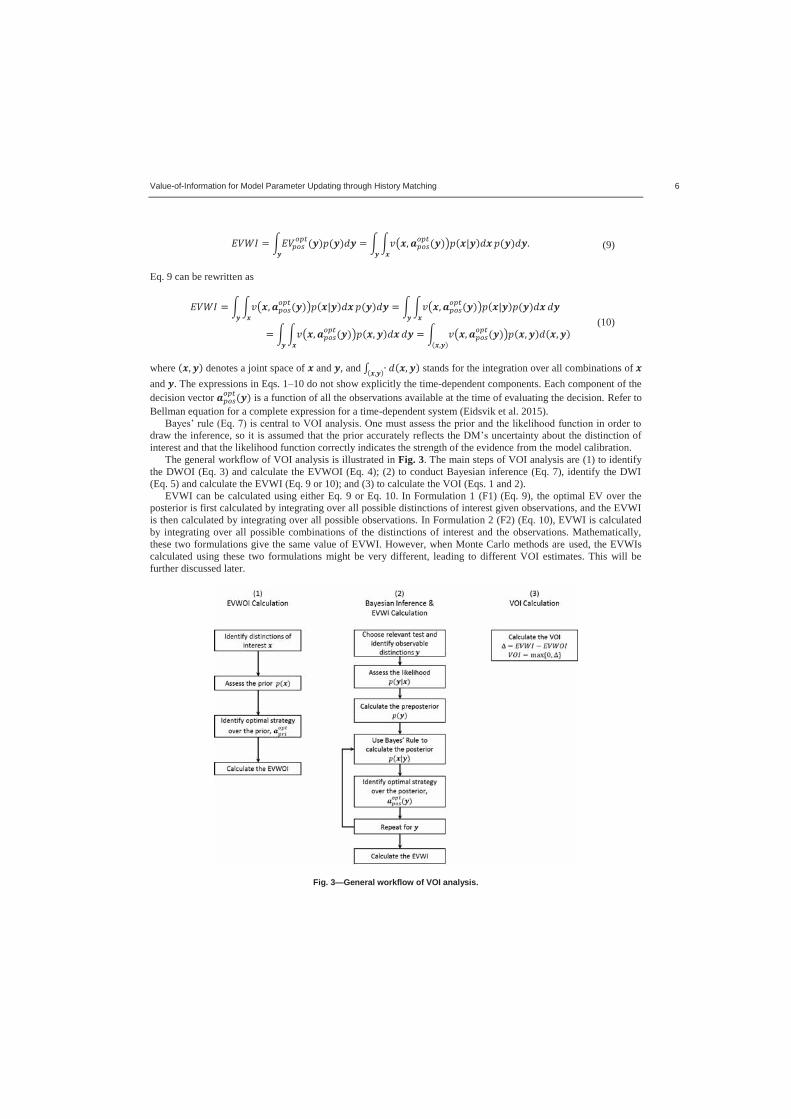
Value-of-Information for Model Parameter Updating through History Matching 6
(9)
Eq. 9 can be rewritten as
(10)
where denotes a joint space of and , and stands for the integration over all combinations of and . The expressions in Eqs. 1 10 do not show explicitly the time-dependent components. Each component of the decision vector is a function of all the observations available at the time of evaluating the decision. Refer to Bellman equation for a complete expression for a time-dependent system (Eidsvik et al. 2015).
draw the inference, so it is assumed that the prior accurately reflects the uncertainty about the distinction of interest and that the likelihood function correctly indicates the strength of the evidence from the model calibration.
The general workflow of VOI analysis is illustrated in Fig. 3. The main steps of VOI analysis are (1) to identify the DWOI (Eq. 3) and calculate the EVWOI (Eq. 4); (2) to conduct Bayesian inference (Eq. 7), identify the DWI (Eq. 5) and calculate the EVWI (Eq. 9 or 10); and (3) to calculate the VOI (Eqs. 1 and 2).
EVWI can be calculated using either Eq. 9 or Eq. 10. In Formulation 1 (F1) (Eq. 9), the optimal EV over the posterior is first calculated by integrating over all possible distinctions of interest given observations, and the EVWI is then calculated by integrating over all possible observations. In Formulation 2 (F2) (Eq. 10), EVWI is calculated by integrating over all possible combinations of the distinctions of interest and the observations. Mathematically, these two formulations give the same value of EVWI. However, when Monte Carlo methods are used, the EVWIs calculated using these two formulations might be very different, leading to different VOI estimates. This will be further discussed later.
Fig. 3 General workflow of VOI analysis.

Value-of-Information for Model Parameter Updating through History Matching 7
There are two essential operations in VOI analysis: Bayesian inference (i.e., calculating the posterior probability distribution) and decision making (i.e., identifying the optimal strategy). Reservoir management decision problems that involve continuous probability distributions and continuous decision spaces require methods other than decision trees for these two steps. EnKF for Bayesian inference and RO for decision making from closed-loop reservoir management are more appropriate methods for building a VOI analysis environment in HM context (Barros et al. 2016a). The following sections will briefly present these two methods. Bayesian Inference with Ensemble Kalman Filter (EnKF) EnKF was introduced by Evensen (1994) as a means to conduct Bayesian inference (Eq. 7) using Monte Carlo methods. The prior probability distribution is represented by a set of realizations of model parameters (i.e., the prior or initial ensemble). The posterior probability distribution is represented by the updated realizations of model parameters (i.e., the posterior or updated ensemble), which are obtained by (Burgers et al. 1998) (11) where matrix consists of the vectors containing the updated states,10 updated model parameters, and updated observations corresponding to each realization in the posterior ensemble; matrix contains the predicted states by forward modelling, model parameters, and predicted observations by forward modelling corresponding to each realization in the prior ensemble; is the Kalman gain matrix, which weighs the influences of the prior predicted observations and the real-time observations (i.e., measurement data); is a matrix containing the perturbed observations; 11 and is an operator that links to the predicted observations. Eq. 11 describes a linear combination of the prior and the observations. The Kalman gain matrix is calculated as (12) where is the covariance matrix of encoding the covariance matrix of the prior predicted observations, and is the covariance matrix of the observations. As the measurements become noisier (i.e., the variance of an observation increases) and/or the variance of a prior predicted observation decreases, more weight is given to the prior; otherwise, more weight is given to the observations.
The EnKF embodies the prior in , the likelihood in (when the model noise is ignored), and the posterior in ; and the preposterior is a norm
among the prior, the likelihood, the preposterior, and the posterior is no longer shown explicitly as in Eq. 7, but is implicitly included in Eq. 11 and 12. A detailed description on the relationship between the formulation of Kalman filter and Bayesian formulation can be found in Meinhold and Singpurwalla (1983). In our case, the inputs of EnKF are the initial guess of the model parameters (i.e., the prior ensemble) together with a model that can predict both the production and observations given a production strategy, observations, and their associated statistics; and the output is the EnKF updated model parameters (i.e., the posterior ensemble). Using EnKF conducted implicitly.
For a comprehensive introduction to EnKF, refer to Evensen (2009). Aanonsen et al. (2009) provided an extensive review of the application of EnKF in reservoir engineering. Decision Making with Robust Optimization (RO) The purpose of HM, and any other information gathering activity, is to acquire information with the aim of improving decision making. This generally requires explicit modeling of the decisions affected by the information obtained from the calibration. This section considers how to optimize the decisions of what water injection strategy to employ. The variables control water injection rates are commonly referred to as the control variables.
The goal of applying RO approach to water injection is to find an optimal strategy (i.e., a set of decisions) that is robust to geological uncertainties (Van Essen et al. 2009). A commonly used measure of the value of a hydrocarbon production project is net present value (NPV). We consider only the revenues from oil production and the costs of
10 Given a dynamic system, a state is an unobservable (in most cases) quantity that must be known currently in order to predict the system behavior (i.e., the future state). A state can be a scalar or a vector. 11 When EnKF is used, an observation has to be perturbed with its corresponding statistics in order to avoid insufficient variance (Burgers et al. 1998).

Value-of-Information for Model Parameter Updating through History Matching 8
water injection and production for a waterflooding case. The NPV for a single geological realization can be calculated by
(13)
where is the value function for decision making; is a vector of uncertain model parameters for a geological realization; is a vector of control variables (i.e., an alternative); is the number of time steps; is the index for time step; the subscripts , , and denote oil, water production, and water injection, respectively; is the injection or production rate over time step length ; , , and are the oil price, water production cost, and water injection cost, respectively; is the discount rate; is the cumulative time for discounting; and is the reference time for discounting. For a risk-neutral DM, the objective function for RO is
(14)
where is the EV of the value function over all realizations, is the index of a realization, and is the number of realizations (i.e., the ensemble size). The objective of RO is thus to find an optimal that maximizes the expected NPV over an ensemble of geological realizations.
For computationally attractive models, the FMINCON-function of MATLAB® (2014) can be used to solve the RO problem. For computationally intensive models, such as a grid-based finite difference or finite element model, ensemble-based optimization approaches such as the EnOpt (Chen et al. 2009) are commonly used to significantly reduce the number of reservoir simulations required for RO and hence reduce the computational costs.
VOI Analysis Using Ensemble-based Methods In ensemble-based methods, a probability distribution is represented by an ensemble, which is a set of realizations. Each realization in the ensemble (i.e., an ensemble member) is equi-probable with a probability of . This is far more tractable than it would be to weight all possible values according to the probability distribution.
The workflow of VOI analysis using ensemble-based methods is illustrated in Fig. 4. This workflow is a modification of the general VOI analysis workflow shown in Fig. 3. The difference between Figs. 3 and 4 is that the probability distribution appears in Fig. 3 are represented by ensembles in Fig. 4.

Value-of-Information for Model Parameter Updating through History Matching 9
Fig. 4 Workflow of VOI analysis using ensemble-based methods. The prior probability distribution is represented by the prior ensemble [ , , ], which consists of
the realizations drawn from . The likelihood function is assessed through a measurement noise distribution. A dynamic system with
model and measurement noise involves the following mathematical relationships:
(15) (16) (17)
where the subscript is the index of time, is a vector of the states, is a vector of the model noise at time ,
is a function that describes the relationship between current states and future states given uncertain parameters and control variables for the period between time and , is a vector of predicted observations at time , is a function that describes the relationship between states and predicted observations,
is a vector of observations (with measurement noise) at time , and is a vector of the measurement noise at time . Combining Eq. 15 and Eq. 16 yields (18) where denotes a forward model that embodies and , is a time-series of control variables from time 0 to time , is the initial state, and encodes the model noise from time 0 to time . If is uncertain, it can be included in ; if it is certain, it can be included in . Thus, Eq. 18 can be simplified to (19)

Value-of-Information for Model Parameter Updating through History Matching 10
For example, when using EnKF together with a reservoir simulation model, standard practice is to assume that the model is accurate (i.e. ) and to assign a multivariate Gaussian distribution to with zero mean and a diagonal covariance matrix (i.e., ); this yields and
, where is referred to as the reliability of the model and as the reliability of measurements, thus . Therefore, as long as the model and measurement noise are assessed and a forward model is given, the likelihood function can be calculated.
The realizations representing the preposterior probability distribution (i.e., the realizations of observations) can be generated by Monte Carlo simulation: (1) sample a realization of the uncertain model parameters from (i.e., the same as generating a realization in the prior ensemble), (2) conduct forward modelling (Eq. 19 with if the model noise is ignored) with to time to obtain a realization of the predicted observations , (3) sample a realization of the measurement noise from , (4) add to (Eq. 17) to obtain a realization of the observations with noise , and (5) repeat (1) (3) to obtain a set of , [ , ], which represents the preposterior. Moreover, the realizations of ( , )-pairs [ , , ] represent the joint probability distribution . In this specific case, we use a 1:1 ratio between and , i.e., for a given , only one realization of is drawn from . One can alternatively use a 1: ratio, i.e., for a given , realizations of are drawn from . This results in a set of with a total of realizations [ , ,
] and a set of ( , )-pairs with a total of realizations [ , , ]. Using a 1:1 ratio is a
simplification that can lead to inaccuracies in the VOI estimate. However, using a 1: ratio requires times more Monte Carlo samples, times increasing the computational cost for the EVWI calculation accordingly. In practice, the measurement noise tends to be quite small (i.e., the standard deviation of is small compared to that of the prior prediction); thus, a 1:1 ratio suffices.
The posterior ensemble [ , ] representing the posterior probability distribution is generated by using EnKF to update the prior ensemble with the given observations and assessed measurement (and model) noise.
With all the probability distributions represented by their corresponding realizations, the VOI analysis can be conducted following the steps presented earlier. The following equations omit the time index for convenience. First, we identify the DWOI and calculate the EVWOI. Converting Eqs. 3 and 4 into their corresponding Monte Carlo forms gives
(20)
(21)
Second, we conduct Bayesian inference, using EnKF to calculate the posterior ensemble members and identify the DWI for the given observations, using the Monte Carlo form of Eq. 5,
(22)
Again, the EVWI can be calculated using either of two formulations: the Monte Carlo form of F1 (Eq. 9),
(23)
or the Monte Carlo form of F2 (Eq. 10),

Value-of-Information for Model Parameter Updating through History Matching 11
(24)
Based on the law of large numbers, Eqs. 23 and 24 give the same limit when the ensemble size approaches infinity. However, the convergence rate can be different, resulting in different estimates when the ensemble size is small. More details on this will be presented with an example later. Finally, we calculate VOI using Eqs. 1 and 2.
Care must be taken when calculating EVWOI and EVWI. If a production optimization problem entails sequential decision making; i.e., the alternative consists of a series of decisions, only the value corresponding to decisions that can be affected by the observations should be considered. For example, if decisions and will be made sequentially at time and , respectively, then an observation obtained somewhere between time and
will affect only and not ,. Therefore, when calculating the value of this observation, only the NPV corresponding to the period from time forward should be considered.
Comparison with s Analysis Workflow Barros et al. (2015a) proposed a workflow for calculating VOI from HM using ensemble-based methods. The authors have extensive experience in reservoir management. However, their paper did not elaborate on the connection between the workflow they have applied and the definition of VOI. This section seeks to accomplish that.
s workflow is based on a twin experiment where the DWI and DWOI are valued based on a synthetic truth and where the difference between the values corresponding to the DWI and DWOI, respectively, is calculated.
s workflow is a realization drawn from the prior probability distribution. realizations are first drawn from the prior probability distribution, and one of them is then chosen as a synthetic truth and the rest form the prior ensemble with realizations. The procedure of conducting a twin experiment is repeated for all
synthetic truths. For each synthetic truth, there is a corresponding difference between its values corresponding to the DWI and DWOI. Barros et al. then calculated the VOI as the EV over all of these differences associated with synthetic truths. Thus, in Ba s workflow, the concept of synthetic truth is central to the analysis.
However, synthetic truth has no meaning in VOI analysis. In reservoir engineering, a synthetically true model is used to mimic the actual state of a reservoir, by which reservoir engineers can investigate whether the actual outcome falls within the range that was predicted by updated models. This is not the case of VOI analysis where the importance is to quantify uncertainty and how the changes in uncertainty will change decisions. Moreover, VOI as defined by Barros et al. implies a distribution.12 However, as shown by Bratvold et al. (2009), the VOI is not a distribution but s workflow is inconsistent with the definition of VOI analysis. However, two small modifications to s workflow can address this.
prior.13 Therefore, the first modification is to not exclude any synthetic truth from the prior ensemble. Because the VOI is defined as the difference between the EVWI and EVWOI, the second modification is to calculate the VOI by first calculating the EV over the values of the DWIs valued on the synthetic truths and the EV over the values of the DWOI valued on the synthetic truths, and then calculating the difference between these two EVs instead of by first calculating the difference between the values of DWI and DWOI valued on a synthetic truth, and then calculating the EV over the synthetic truths. Although the second modification is only formula rewriting and causes no difference in mathematical result, it makes conceptual difference. s workflow is identical to calculating the VOI using F2. Because F2 is derived without introducing the concept of synthetic truth, there is no need to include the concept of synthetic truth in VOI analysis.
r engineers, whilst F2 is from the original definition of VOI. similarity of it to F2 provides
an easier understanding of the VOI from HM for reservoir engineers. The differences among F1, F are summarized in Table 2. The impact of using the
three approaches will be illustrated and discussed later.
12 Barros et al. (2015a, 2015b, 2016a) illustrated the percentiles of VOI. 13 As is common in VOI analysis, this work assumes that the probability assessors are unbiased.

Value-of-Information for Model Parameter Updating through History Matching 12
Index Formulation 1 Formulation 2 Barros et al.
1
DWOI is identified and EVWOI is calculated over all
prior realizations (Eqs. 20 and 21).
DWOI is identified and EVWOI is calculated over all
prior realizations (Eqs. 20 and 21).
DWOI is identified by optimizing the EV over prior realizations after a synthetic truth is excluded. The DWOI is valued on the synthetic truth, i.e., value without information for the synthetic truth ( ) is calculated. This procedure is repeated for all synthetic truths.
2 All prior realizations are updated, resulting in posterior realizations.
All prior realizations are updated, resulting in posterior realizations.
prior realizations are updated, resulting in posterior realizations.
3 DWI is identified over posterior realizations (Eq. 22).
DWI is identified over posterior realizations (Eq. 22).
DWI is identified over posterior realizations.
4 EVWI is calculated using Eq. 23.
EVWI is calculated using Eq. 24.
The value with information for each particular synthetic truth ( ) is calculated.
5 VOI is calculated as the difference between EVWI and EVWOI.
VOI is calculated as the difference between EVWI and EVWOI.
The VOI for each synthetic truth ( ) is calculated as , and the VOI is calculated as the EV of .
Table 2 Decision Tree Example The following is a simple illustration of how decision trees can be used to assess the VOI in the HM context. For an introduction to decision trees and tree flipping, refer to Clemen (1991), Bratvold and Begg (2010), and Howard and Abbas (2016).
Assume that the prior has been assessed as three equi-probable sets of uncertain model parameters of a given production model: , , and . We want to estimate the value of measuring and calibrating to the oil production rate at time . The predicted oil production rates by these three realizations are shown in Fig. 5, where is the oil production rate predicted for the period from time 0 to , which is obtained from the production model with parameters and production strategy . It is assumed that there is no model noise. For example, if describes the true nature of the reservoir, is the production strategy and there is no measurement noise, the observed oil production rate will definitely be at time (i.e., any given set of values of model parameters maps to only one set of predicted observations a one-to-one relationship). Thus, we have the following model reliabilities:
else 0. However, the relationship from predicted observations to model parameters might not be one-to-one, because of non-uniqueness of inverse modelling. For example, given , the corresponding set of model parameters can be either or . The reliabilities of the measurements are listed in Table 3. For example, given the oil production rate is low ( ), the probability of the measurement providing an exact ) is 4/5 and that of a deviated ) is 1/5. Given the reliabilities of the model and measurements, we can calculate the likelihoods. For example,
. The likelihood function is listed in Table 4. The preposterior and posteriors are calculated using Eq. 8 and 7, respectively.

Value-of-Information for Model Parameter Updating through History Matching 13
Fig. 5 The oil production rate profiles of three equi-probable realizations for the decision tree example.
Reliabilities of Measurement
(says|is) Given at time is Low ( ) High ( )
at time says ) 4/5 1/5 ) 1/5 4/5
Total 1 1
Table 3 Reliabilities of measurement for the decision tree example.
Likelihood Function (says|is)
Given the set of model parameters is
at time says ( ) 4/5 4/5 1/5
) 1/5 1/5 4/5 Total 1 1 1
Table 4 Likelihood function for the decision tree example.
Fig. 6a shows the probability tree with the prior and likelihoods in the assessed form. Its corresponding
inferential form (flipped tree) is shown in Fig. 6b, where the preposterior and posteriors are listed.
(a) Assessed Form: Information we have (b) Inferential Form: Information we need
Fig. 6 The uncertainty trees in (a) assessed form, and (b) inferential form for the decision tree example. Because information cannot add value if it is not material, we must define the decision context before the VOI
can be calculated. This example will assume that we can choose one of three production strategies, denoted by , and , that the strategies are the same for the time interval through , and that they differ for the remaining
period. Thus, we have two options: (1) to choose from , and based on the prior (i.e. the case without information), and (2) to measure the oil production rate at time and then, to choose from , and based on the measurement (i.e. the case with information). Let be the NPV of the project for the period from time to the end of the production life-cycle, calculated with realization and decision . The NPVs for different alternatives and realizations are listed in Table 5. The decision trees for the cases with and without information are shown in
( )

Value-of-Information for Model Parameter Updating through History Matching 14
Fig. 7, where the triangles represent payoffs or values. These trees show only the branches for the optimal decision, i.e., the alternative that maximizes the expected NPV. Recall that the VOI is assessed before any information is gathered. The decision tree in Fig. 7b includes the observation uncertainty to the left of the decision nodes.
89 56 49 73 64 65 75 6 88
Table 5 NPVs for different alternatives and realizations [$ millions] for the decision tree example.
(a) Without Information (b) With Information
Fig. 7 The decision trees for the cases (a) with information, and (b) without information for the decision tree example.
As shown in Fig. 7a, the DWOI is , the EVWOI is $67.3 million, and the EVWI is $70.8 million. The EVWI
can be calculated using either F1 (Eq. 9):
or F2 (Eq. 10):
The VOI is $70.8 $67.3 = $3.5 million. If the cost of measurement is greater than $3.5 million, the measurement of oil production rate should not be conducted; otherwise, the oil production rate should be measured. The value increment of $3.5 million comes from the possible change in DWI. The optimal decision is alternative for the case without information, whereas it is ) or if the measurement says
). If irrespective of the information, is retained for the decision nodes in Fig. 7b, this will yield and thus , which means that the information has no value if it cannot change our
decision. The VOI of the case without noise in measurement (i.e., , else 0) is $10.4
million. The VOI of the case with perfect information (VOPI) is $13.0 million. The VOI increment from $3.5 million to $10.4 million is due to the elimination of measurement noise. The difference between the VOI without measurement noise ($10.4 million) and VOPI ($13.0 million) is because having data does not provide perfect
( )

Value-of-Information for Model Parameter Updating through History Matching 15
information about the future production even though the data have no noise. This imperfection can be ascribed to the non-uniqueness of inverse modelling. If a given dataset mapped to only one set of model parameters (i.e.,
for all ), then the dataset would provide perfect information. Monte Carlo Example with a Static Model Assessing the VOI for the example above is straightforward because it is a discretized case having a single uncertainty with only three possible outcomes. In practice, many hydrocarbon production relevant decision making contexts involve continuous probability distributions (e.g., an uncertain permeability field can be a multivariate Gaussian distribution). Monte Carlo method uses a number of equi-probable realizations to represent a continuous probability distribution. A disadvantage of Monte Carlo method is that it can result in sampling errors, which could for example cause the EVWIs calculated using F1 (Eq. 23) and F2 (Eq. 24) to differ. This section presents an example where a simple static model is used so that the VOI can be easily calculated analytically. This VOI will then be compared with those s workflow, F1, and F2.
Consider that the distinction of interest is the revenue of a project and that the observable distinction is the information on the revenue. The relationship between and is (25) where is normally distributed with mean and standard deviation , and is normally distributed with zero mean and standard deviation : the prior and the likelihood . The error term in Eq. 25 describes the reliability of the information. Using the relationships for the normal conjugate prior, the preposterior is
and the posterior is . The decision to be
made is whether the project will be conducted; and respectively. If the expected revenue is positive, the project should be conducted; otherwise, it should not. Thus, the value function is . The DM wants to know whether the information should be obtained against a cost of 1 (the monetary unit can be arbitrary here).
The VOI for this case can be calculated analytically:
(26)
With , , and , the VOI is 2.267. Because the cost of information is lower than the VOI, the DM should buy the information.
For comparison, we use Monte Carlo method to calculate the VOI. First, we sample realizations from the prior to get the prior ensemble [ , ], with the probability of each being . Second, the DWOI is obtained using Eq. 20, and the EVWOI is calculated using Eq. 21. Third, for each , we sample one realization from the likelihood to get the preposterior ensemble [ , ], with the probability of each being
as well as an ensemble of ( )-pairs, [ , ], with the probability of each ( , )-pair being (the 1:1 ratio mentioned earlier applies here). Fourth, we update the prior ensemble using EnKF for each , yielding the posterior ensemble [ , ], and we identify the DWI using Eq. 22; this results in posterior ensembles and DWIs. Fifth, the EVWI can be calculated using either F1 (Eq. 23) or F2 (Eq. 24). Finally, we calculate the VOI using Eqs. 1 and 2.
s workflow, F1 and F2 using a large ensemble size of 10,000. The results are listed in Table 6, where s workflow gives a result almost identical to that of F2. This is because the impact of excluding a synthetic truth (i.e., an ) from the prior ensemble is very small when the ensemble size is large. The VOIs calculated using F1 and F2 are slightly different, for a reason to be discussed later. All three methods estimate the VOI with an error smaller than 1%.

Value-of-Information for Model Parameter Updating through History Matching 16
Method VOI
Error
Analytical
2.267 -
s Workflow
2.283 0.71%
Formulation 1
2.246 0.93%
Formulation 2
2.283 0.71%
Table 6 VOI estimate with , , , and an ensemble size of 10,000 for the Monte Carlo example with a static model.
Then, a small ensemble size of 50 is used. The VOI calculation is repeated 10,000 times for each method. The
statistics of the VOI estimates are listed in Table 7, and the probability density functions (PDFs) are plotted in Fig. 8.14 Both F1 and F2 are shown to produce a VOI estimate with an error smaller than 0.5% on average. F2 leads to a smaller standard deviation (SD) of the VOI estimate than does F1. This indicates that F2 is more stable than F1 with respect to Monte Carlo sampling for small ensemble size because of s sole use of the prior ensemble for calculating EVWI, thereby excluding from that calculation the sampling errors associated with the preposterior and posterior ensembles. In contrast, F1 uses both the preposterior and posterior ensembles for the EVWI calculation, thereby propagating sampling errors from the preposterior and posterior ensembles. s workflow, the resulting range and SD of VOI estimate are larger than in the other two methods, and the PDF includes a long tail to the right as shown in Fig. 8, resulting in a larger error for the average VOI estimate. This long tail is induced by the exclusion of the synthetic truths from the prior ensemble. This suggests that the impact of excluding the synthetic truths from the prior ensemble can be large when the ensemble size is small. In reservoir management, small ensemble size is usually used for EnKF, typically 100, as the computational costs increase with the ensemble size.
Method Average
Error SD [Min, Max]
2.323 2.47% 0.933 [0, 10.421]
Formulation 1
2.257 0.44% 0.776 [0, 5.497]
Formulation 2
2.259 0.35% 0.695 [0, 5.279]
Table 7 VOI estimate with , , , and an ensemble size of 50 (repeated 10,000 times) for the Monte Carlo example with a static model.
Fig. 8 The PDF of VOI estimate for the Monte Carlo example with a static model.
This example has demonstrated that the three methods give almost equivalent results for large ensembles.
However, these methods can lead to quite different results when the ensemble size is small. As there are no significant computational increases resulting from F2 (Eq. 24) for calculating the VOI from HM when Monte Carlo is used, this would be our method of choice. 14 The uncertainty in the VOI estimate is due to the sampling error associated with Monte Carlo method. As discussed earlier, the VOI itself is not a distribution but the difference between two expected values.

Value-of-Information for Model Parameter Updating through History Matching 17
Monte Carlo Example with a Toy Dynamic Model This section illustrates how the VOI from HM is calculated. We adopt the decline curve model used by Barros et al. (2016a) for modeling oil and water production. The predicted oil and water production rates, and , respectively, are functions of time and a control (decision) variable ,:
(27)
(28)
where is the initial oil production rate for ; is the ultimate water production rate for ; is the water breakthrough time for ; , , , , and are coefficients; is the average of in all the control intervals before ; and is the Heaviside step function. The water injection rate is the sum of and
. The constants and uncertain model parameters are listed in Table 8. The production life-cycle is 80 months, and . We include eight control intervals, and the single control variable is thus replaced by a control vector . That is, when a decision is made at time , it cannot be changed over the next 10 time intervals. The upper and lower bounds of are 10 bbl/mo and 50 bbl/mo, respectively. The observations are oil and water production rates at a certain time. In the form of Eqs. 19 and 17, we have the distinctions of interest , predicted observations , observations (with noise) , and a forward model to time , described by Eqs. 27 and 28.
Constant Parameters Uncertain Parameters 0.1 [ - ] N(100, 8) [bbl/mo] 4 [bbl/mo2] N(30.5, 3.67) [mo] 150 [bbl/mo] N(132, 6) [bbl/mo] 2 [ - ] N(32, 6) [mo] 1.33 [bbl/mo2] 70 [$/bbl] 10 [$/bbl] 10 [$/bbl]
0.1 [ - ] 8 [mo]
Table 8 Constant and uncertain parameters for the decline curve model.
We use a Gaussian distribution for the reliability of measurements, i.e., where
, with and being the SDs of oil and water rate measurements, respectively. For this example, we
assume that the SD is a percentage of the EV of the prior predicted observation (i.e., ) for both the oil and water production rates, and set . Model noise is ignored.
An ensemble size of 100 is used. Realizations are sampled from the prior (Gaussian distributions listed in Table 8) to form the prior ensemble [ , ]. RO is performed over the prior ensemble to identify the optimal strategy (i.e., DWOI) that optimizes the EV over the prior ensemble (Eq. 20).
The VOI calculation will be for information gathered at time . For a sequential decision making context, the information gathered at time will affect the decisions made only after the time when we gather the information. Thus, we care about the value only for the period where decisions are changeable, and the value function should be defined as the NPV for that period. For example, decisions that can be affected by information gathered at time
, are { , }, so we consider the value function for only the period after time . All monetary values are discounted to time 0.
We first do forward modeling to time with the prior ensemble members and DWOI to generate the realizations of the predicted observations [ , ] and then sample one realization of measurement noise from and add it to to obtain [ , ] which is the

Value-of-Information for Model Parameter Updating through History Matching 18
preposterior ensemble. For each , we use EnKF to update the prior ensemble to obtain the posterior ensemble [ , ] and perform RO over the posterior ensemble to identify the optimal strategy after time for the posterior ensemble. Again, using information gathered at time as an example, the DWI after time
is . The EVWOI can then be calculated using Eq. 21, and the EVWI using F1 (Eq. 23) or F2 (Eq. 24). The VOI is
calculated using Eqs. 1 and 2. Both F1 and F2 are used to calculate the defined in Eq. 2. From Eq. 1, . The calculation of
at time using our proposed workflow is repeated 100 times for each formulation. The ensembles used in any two runs are different. The statistics of the estimates are listed in Table 9.15 As was found in the previous example, the average of the estimates calculated using F1 is close to that of F2; however, the SD of the estimates calculated using F1 is much larger than that of F2, due to the small ensemble size. Different VOI estimates can lead to different decisions. Taking one of the 100 runs as an example, we get a VOI estimate of $621.4 using F1 and $107.6 using F2, even though the same set of realizations is used; if the cost of gathering data and conducting model calibration is $150, the decision made based on the VOI calculated using F HMthe decision made based on that using F In practice, because we want to minimize the computational cost. Thus, the formulation which has the higher chance to produce a good estimate (i.e. smaller SD in estimate) should be used.
Method Average
SD [Min, Max]
Formulation 1
64.7 480.3 [-1181.9, 1049.6]
Formulation 2
58.4 31.5 [-64.6, 148.8]
Table 9 Statistics of the for the Monte Carlo example with a dynamic model.
We use F2 to calculate the VOI at different times using the same prior ensemble, to answer the following
questions: (1) If we can conduct the measurements of oil and water production rates only once at some time during the production life-cycle (i.e., we can get only a single value of ), when should this be done? (2) How much value can be created by the measurements? Repeating the VOI calculation for data gathered at different times yields the graph shown in Fig. 9. It indicates that the value of imperfect information with peaks at time 30 with a value of $217.5. If the cost of gathering data and conducting model calibration is less than $217.5, we should gather data and conduct model calibration at time 30; otherwise, we should not gather data at all. The value that can be created by the measurements is the difference between its VOI and cost. For example, if the cost is $118, then the created value is $217.5 $118 = $99.5. The VOPI is the upper bound of VOI. Not surprisingly, the graph indicates that if we have access to perfect information, we should gather data as soon as possible (between time 0 and 10) if the information can be obtained at a cost of no more than $674.3. There are sharp drops in both VOI with measurement noise and VOPI at time 11, 21, 31 and 41. This is because one more decision in the series of decisions of production strategy cannot be affected by the data gathered at these times (Barros et al. 2016a). For example, the injection rate decision for the period from time 20 to 30 is made at time 20, so the data gathered before time 20 can affect this decision whilst the data gathered after time 20 cannot affect this decision but only the decisions made after that.
15 See footnote 14.

Value-of-Information for Model Parameter Updating through History Matching 19
Fig. 9 VOI with and VOPI at different times for the Monte Carlo example with a dynamic model.
How would different levels of measurement noise impact VOI? To investigate this, we conducted a sensitivity
analysis of the measurement noise (i.e., the value of ) on VOI. VOI at different times is shown for three values of (1%, 5%, and 9%) in Fig. 10. The smoothness of the curve decreases with increasing measurement noise. We believe this is because of the sampling errors associated with sampling the measurement noise. As the measurement noise increases, larger sampling errors will be introduced when the measurement noise is sampled using the same ensemble size for Monte Carlo method, resulting in larger errors in VOI estimate. Fig. 10 shows that VOI increases as decreases, and that the VOI peaks at time 30 no matter how large is. This is because water break-through will have occurred over the majority of the realizations at time 30, and the water rate data gathered at this time provides relevant and material information on the future water production. Thus, we focus on VOI at time 30 and calculate it for different values of . The results, shown in Fig. 11, indicate that as measurement noise increases, VOI approaches 0 (i.e., the information is immaterial). Because the measurement noise tends to be quite small in practice, we consider only between 0% and 22% for further analysis. The VOI estimates are indicated by blue dots in Fig. 12, and the red dashed line is the second-order polynomial trendline corresponding to the VOI estimates. The cost of reducing measurement noise is represented by the green solid line in Fig. 12, showing that VOI and the cost intersect at . For , the measurement cost is greater than the VOI, indicating that paying for a more accurate measure does not add value. For , the measurement cost is lower than the VOI. The difference between VOI and cost is shown in Fig. 13. The information value increases as increases until it reaches 9.1%, corresponding to an optimal value of $105.8 (the red dot in Fig. 13). The sensitivity analysis indicates that a more accurate measure does not necessarily create more value and that a tradeoff exists between measurement accuracy and costs.
Fig. 10 VOI at different times for different levels of
measurement noise for the Monte Carlo example with a dynamic model.
Fig. 11 VOI at time 30 for different levels of measurement noise for the Monte Carlo example with a
dynamic model.

Value-of-Information for Model Parameter Updating through History Matching 20
Fig. 12 VOI at time 30 and measurement cost for
different levels of measurement noise for the Monte Carlo example with a dynamic model.
Fig. 13 VOI at time 30 less measurement cost for different levels of measurement noise for the Monte
Carlo example with a dynamic model. Monte Carlo Example with a Reservoir Simulation Model We use our proposed workflow to estimate VOI from HM for a more realistic case where a reservoir simulation model is involved. The reservoir simulation model (a synthetic 2D model) is shown in Fig. 14. Eight injectors are placed in line at one end of the reservoir and eight producers in line at the opposite end. The permeability field is uncertain and its prior uncertainty is described by a multivariate normal distribution. The prior ensemble consists of 50 realizations sampled from the prior distribution, 3 of which are illustrated in Fig. 15.
Fig. 14 Synthetic 2D model for the Monte Carlo example with a reservoir simulation model.
Fig. 15 Three of 50 sampled realizations of the permeability field in md.
We assume that the periods of water pre-flushing, polymer injection and water post-flushing have already been
set: 1,200 -water post-flushing. The injection rate is fixed at 15 m3/day for each injector and the producer bottom hole pressure is fixed at 200 bars for each producer. At the end of water pre-flushing, the DM needs to decide what polymer concentration should be used in each injector for the whole period of polymer injection. Thus, there are totally 8 control variables. The polymer concentration is bounded between 0 kg/m3 and 6.5 kg/m3.
Oil and water production rates in each producer will be measured every 240 days during the water pre-flushing period. These data can be used for HM and inform the decision on polymer concentration. In addition to oil and water production rate data, the DM is considering to gather another type of data: water saturations in the grid-blocks circled by the red rings in Fig. 14 by placing saturation measuring devices at these locations. If the devices are placed, water saturations in these grid-blocks will be measured every 240 days as well. The questions are: What is the value of additional water saturation data? Should the saturation measuring devices be placed?

Value-of-Information for Model Parameter Updating through History Matching 21
The value function is defined as the NPV with revenue from oil production and costs for water production, water injection and polymer injection, i.e.,
(29)
where is the total polymer injection rate over time step length and is the polymer injection cost. The parameter values used in this specific example are listed in Table 10.
220 $/m3 47.5 $/m3 12.5 $/m3 12 $/kg
8% 365 days 30 days
Table 10 Parameter values for NPV calculation in the Monte Carlo example with a reservoir simulation model.
The measurement noise of oil and water production rate is assumed to be normally distributed with zero mean and a SD of 1 m3/day, and the measurement noise of water saturation to be normally distributed with zeros mean and a SD of 0.01. Model noise is ignored.
VOI is calculated using our proposed workflow combined with EnKF and EnOpt. The resulting VOIs for rate data only, saturation data only, and both rate and saturation data, and VOPI are listed in Table 11.
Data Type Rate Saturation Rate and Saturation
Perfect Information
VOI 5]
3.10 3.36 4.11 6.12
Table 11 VOI estimates for Monte Carlo Example with a Reservoir Simulation Model. It can be see that the values of rate data and saturation data are very close to each other. Although the saturation
data has a value of $3.36 5 when it is considered individually, it adds a value of only $1.01 5 (= $4.11 5 $3.10 5) in addition to rate data. This indicates that VOI is not additive (Samson et al. 1989). The VOI analysis informs the DM that he/she should not gather saturation data in addition to rate data if the cost of placing saturation measuring devices is greater than $1.01 5. Discussion and Conclusions This paper has introduced a workflow for calculating VOI from HM and that is consistent with the original definition of VOI in the decision sciences. The workflow employs ensemble-based methods and Monte Carlo sampling. Two formulations (F1 and F2), both of which are consistent with VOI analysis, can be used to calculate the EVWI. In the limit where the ensemble size approaches infinity, the EVWIs calculated using these two formulations are identical. However, the numerical results may be different, and consequently different VOI estimates will be calculated when the ensemble size is small. The VOI calculated using F2 is less sensitive with regard to ensemble size than is F1. F2 is thus our method of choice for calculating the VOI from HM using Monte Carlo method.
F s workflow. We noted that s workflow, which relies on twin experiments, is inconsistent with VOI analysis because VOI is a value, not a distribution. Nevertheless, two small modifications to s workflow will make it consistent with VOI analysis and consequently, equivalent to F2.
A decision tree was used to illustrate the implementation of the general workflow for VOI analysis in HM contexts The use of decision trees provides clarity in communicating the detailed steps for VOI analysis.
We conducted a sensitivity analysis of the impact of different levels of measurement noise. Due to the non-uniqueness inherent in the HM inverse problem, a zero measurement noise will not result in perfect information about future production. As the measurement noise increases, VOI is reduced; and once measurement noise exceeds a threshold, the gathered production data will be immaterial and thus worthless. The sensitivity analysis thus

Value-of-Information for Model Parameter Updating through History Matching 22
confirmed that applying the ensemble-based approach for HM in a VOI framework is consistent with classical VOI analysis. The sensitivity analysis also illustrated that the value of a measure (its VOI less its cost) does not necessarily increase as measurement accuracy is improved.
Two Monte Carlo examples demonstrated the application of F2 for VOI assessment. The first example analyzed the optimal timing of conducting data measurement, and the second example investigated the value of obtaining additional type of data.
Although we used EnKF for HM (Bayesian updating) and EnOpt for RO (decision making), the proposed VOI workflow could employ any Bayesian updating method or optimization method. The performance of the calibration method can affect the accuracy of VOI assessment. EnKF is derived from the Kalman filter, which is designed for Gaussian distributions. Thus, any inherent non-Gaussianity (e.g., value truncation) can introduce errors in Bayesian updating and consequent errors in the VOI calculation. When VOI is calculated using Monte Carlo method, the number of realizations used to represent the probability distributions affects the accuracy of the VOI calculation. We used an ensemble size of 100, which has been regarded as a reasonable compromise between fairly representing the probability distribution and limiting computational costs for EnKF. However, given that Bickel (2012) showed that more than 1,000 realizations are required for a good estimate of VOI in a case where only one uncertain quantity is involved, an ensemble size of 100 is unlikely to provide an accurate assessment of VOI from HM. The accuracy of VOI estimate using EnKF and EnOpt should be further investigated in future reseach.
A significant constraint on the routine use of VOI in the HM context is its high computational cost (Barros et al. 2016a). An ensemble size of , would entail ensemble-based HM and optimizations over all realizations. If a production model needs hours to run, as in many real cases, the CPU time for assessing the VOI for observations obtained at a certain time will be years. Thus, using parallel computing for VOI calculation can significantly reduce the waiting time because both the EnKF and RO parts of the workflow can be done in parallel across realizations. If parallel computing is unavailable, one possible approach is to use fast proxy models (e.g., an upscaled model or a decline curve model) for production modeling. If this can reduce model run time from hours to seconds, the CPU time would be reduced from years to hours, making it acceptable for a practical setting. Another possible solution is to reduce the number of realizations using an efficient discretization method (Bratvold and Thomas 2014). This works well when only a few uncertain quantities are involved. However, this approach can also be computationally very expensive when numerous uncertain quantities are involved because the number of discretization points increases exponentially with the number of uncertain quantities. Barros et al. (2016b) reduced the number of realization needed using clustering techniques to select representative models from an ensemble.
The computational cost is even higher for a sequential decision making context. Because of this, we only illustrated VOI assessment for the case with only one decision point. Although Barros et al. (2015b) has extended their workflow to incorporate sequential decisions using the closed loop reservoir management (CLRM) approach, we argue that CLRM is a myopic or naïve decision policy where the uncertainties associated with current available data is considered but the uncertainties associated with future data is not. Fig. 16 illustrates the decision tree representation for CLRM. The advantage of CLRM is that it greatly simplifies the structure of a sequential decision making problem and consequently, requires less computational cost for solving the problem. Its significant drawback is that it does not reflect the full structure of a sequential decision making problem and thus, may lead to a sub-optimal production strategy. Fig. 17 illustrates the decision tree representation for the full structure of a sequential decision making problem. The full structure explicitly considers both the uncertainties associated with current available data and that with future data, i.e., it allows for learning over time. Therefore, the current decision does not depend on only the uncertainties that a decision maker have learnt so far but also the uncertainties that the decision maker will learn in the future. Solving the fully structured decision tree gives the optimal production strategy. Per the strict definition of VOI, it is referred exclusively to that associated with the optimal decision policy (i.e. the solution of the fully structured decision tree). The VOI assessed using the CLRM approach is a special case and only for the CLRM production strategy. The VOI associated with the CLRM production strategy may be lower than the generally defined VOI (i.e. the VOI associated with the optimal production strategy). Therefore, using the CLRM approach is a simplification of solving a sequential decision making problem but not a replacement. Solving for the optimal production strategy may create more value than the CLRM production strategy but requires more computational cost.

Value-of-Information for Model Parameter Updating through History Matching 23
Fig. 16 Decision tree representation for CLRM.
Fig. 17 Decision tree representation for the full structure of a sequential decision making problem.
Another significant constraint is the difficulty in Bayesian inference when a large number of uncertain
parameters (e.g., the porosity and permeability in each grid block of a reservoir simulation model) is involved. Although many publications have shown promising results of updating a large number of uncertain parameters using EnKF, it may lead to statistic bias and consequently reduce the accuracy of VOI calculation. Any other Bayesian updating methods, e.g., the ensemble smoother (Skjervheim and Evensen 2011) or Markov-chain Monte Carlo methods (Oliver et al. 1997), can be adopted into our proposed workflow. Thus, a possible direction for further research is to investigate the impact of different updating methods on VOI estimate.
Many producing fields and most new fields gather some types of data (e.g., water, oil, and gas production rate and well bottom-hole pressure) for monitoring and other purposes. VOI analysis plays no role for these types of measurements, because the data already have been or definitely will be gathered. However, VOI analysis is very relevant and useful for other types of costly data, such as 4D seismic surveys.
Although issues remain in the context of developing a broad and deep understanding and routine application of the concept, we remain optimistic about the value of VOI analysis in the O&G industry.
Acknowledgements The authors acknowledge the support of the Research Council of Norway and industry partners: ConocoPhillips, Skandinavia AS, BP Norge AS, Det Norske Oljeselskap AS, Eni Norge AS, Maersk Oil Norway AS, DONG Energy A/S, Denmark, Statoil Petroleum AS, ENGIE E&P NORGE AS, Lundin Norway AS, Halliburton AS, Schlumberger Norge AS, and Wintershall Norge AS of The National IOR Centre of Norway. References Aanonsen, S. I., Nævdal, G., Oliver, D. S. et al. 2009. The Ensemble Kalman Filter in Reservoir Engineering a
Review. SPE Journal 14 (3): 393 412. SPE-117274-PA. http://dx.doi.org/10.2118/117274-PA. Aylor, W. K. Jr. 1999. Measuring the Impact of 3D Seismic on Business Performance. Journal of Petroleum
Technology 51 (6): 52 56. SPE-56851-JPT. http://dx.doi.org/10.2118/56851-JPT. Barros, E. G. D., Jansen, J. D., and Van den Hof, P. M. J. 2015a. Value of Information in Parameter Identification
and Optimization of Hydrocarbon Reservoirs. IFAC-PapersOnLine 48 (6): 229 235. http://dx.doi.org/10.1016/j.ifacol.2015.08.036.
Barros, E. G. D., Leeuwenburgh, O., Van den Hof, P. M. J. et al. 2015b. Value of Multiple Production Measurements and Water Front Tracking in Closed-Loop Reservoir Management. Presented at the SPE Reservoir Characterisation and Simulation Conference and Exhibition, Abu Dhabi, UAE, 14 16 September. SPE-175608-MS. http://dx.doi.org/10.2118/175608-MS.
Barros, E. G. D., Van den Hof, P. M. J., and Jansen, J. D. 2016a. Value of Information in Closed-Loop Reservoir Management. Computational Geosciences 20 (3): 737 749. http://dx.doi.org/10.1007/s10596-015-9509-4.
Barros, E. G. D., Yap, F. K., Insuasty, E., Van den Hof, P. M. J., and Jansen, J. D. 2016b. Clustering Techniques for Value-of-information Assessment in Closed-loop Reservoir Management. Presented at ECMOR XV 15th European Conference on the Mathematics of Oil Recovery, Amsterdam, Netherlands, 29 August 1 September. http://dx.doi.org/10.3997/2214-4609.201601858.

Value-of-Information for Model Parameter Updating through History Matching 24
Bickel, J. E. 2012. Discretization, Simulation, and the Value of Information. SPE Economics & Management 4 (4): 198 203. SPE-145690-PA. http://dx.doi.org/10.2118/145690-PA.
Bratvold, R. B., and Begg, S. 2010. Making Good Decisions, first edition. Texas, USA: Society of Petroleum Engineers.
Bratvold, R. B., Bickel, J. E., and Lohne, H. P. 2009. Value of Information in the Oil and Gas Industry: Past, Present, and Future. SPE Reservoir Evaluation & Engineering 12 (4): 630 638. SPE-110378-PA. http://dx.doi.org/10.2118/110378-PA.
Bratvold, R. B., and Thomas, P. 2014. Robust Discretization of Continuouos Probability Distributions for Value-of-Information Analysis. Presented at the International Petroleum Technology Conference, Kuala Lumpur, Malaysia, 10 12 December. IPTC-17975-MS. http://dx.doi.org/10.2523/IPTC-17975-MS.
Burgers, G., Jan van Leeuwen, P., and Evensen, G. 1998. Analysis Scheme in the Ensemble Kalman Filter. Monthly Weather Review 126 (6): 1719 1724. http://dx.doi.org/10.1175/1520-0493(1998)126<1719:ASITEK>2.0.CO;2.
Chen, Y., Oliver, D. S., and Zhang, D. 2009. Efficient Ensemble-Based Closed-Loop Production Optimization. SPE Journal 14 (4): 634 645. SPE-112873-PA. http://dx.doi.org/10.2118/112873-PA.
Clemen, R. T. 1991. Making Hard Decisions: An Introduction to Decision Analysis. Boston, USA: PWS-Kent. Coopersmith, E. M., Burkholder, M. K., and Schulze, J. H. 2006. Value-of-Information Lookbacks Was the
Information You Gathered Really Worth Getting? Presented at the SPE Annual Technical Conference and Exhihition, San Antonio, Texas, USA, 24 27 September. SPE-101540-MS. http://dx.doi.org/10.2118/101540-MS.
Eidsvik, J., Mukerji, T., and Bhattacharjya, D. 2015. Value of Information in the Earth Sciences: Integrating Spatial Modeling and Decision Analysis, first edition. Cambridge, United Kingdom: Cambridge University Press.
Eppel, T., and von Winterfeldt, D. 2008. Value-of-Information Analysis for Nuclear Waste Storage Tanks. Decision Analysis 5(3): 157 167. http://dx.doi.org/10.1287/deca.1080.0121.
Evensen, G. 1994. Sequential Data Assimilation with a Nonlinear Quasi Geostrophic Model Using Monte Carlo Methods to Forecast Error Statistics. Journal of Geophysical Research: Oceans 99 (C5): 10143 10162. http://dx.doi.org/10.1029/94JC00572.
Evensen, G. 2009. Data Assimilation: The Ensemble Kalman Filter, second edition. Heidelberg, Germany: Springer Science & Business Media.
Grayson, C. J. Jr. 1960. Decisions under Uncertainty: Drilling Decisions by Oil and Gas Operators. Boston, Massachusetts: Harvard University Press.
Howard, R. A. 1966. Information Value Theory. IEEE Transactions on Systems Science and Cybernetics 2 (1): 2226. http://dx.doi.org/10.1109/TSSC.1966.300074.
Howard, R. A., and Abbas, A. E. 2016. Foundations of Decision Analysis, global edition. Harlow, England: Pearson Education Limited.
Krymskaya, M. V., Hanea, R. G., Jansen, J. D. et al. 2010. Observation Sensitivity in Computer-Assisted History Matching. Presented at the 72nd EAGE Conference and Exhibition incorporating SPE EUROPEC 2010. http://dx.doi.org/10.3997/2214-4609.201400961.
Le, D. H., and Reynolds, A. C. 2014. Optimal Choice of a Surveillance Operation Using Information Theory. Computational Geosciences 18(3 4): 505 518. http://dx.doi.org/10.1007/s10596-014-9401-7.
MATLAB® Software 2014. Version 8.4.0.150421 (R2014b). Meinhold, R. J., and Singpurwalla, N. D. 1983. Understanding the Kalman Filter. The American Statistician 37 (2):
123 127. Oliver, D. S., Cunha, L. B., and Reynolds, A. C. 1997. Markov Chain Monte Carlo Methods for Conditioning a
Permeability Field to Pressure Data. Mathematical Geology 29(1): 61 91. https://doi.org/10.1007/BF02769620.
Raiffa, H., and Schlaifer, R. 1961. Applied Statistical Decision Theory. Boston: Division of Research, Graduate School of Business Administration, Harvard University (Reprint).
Schlaifer, R. 1959. Probability and Statistics for Business Decisions. New York: McGraw-Hill. Skjervheim, and Evensen, G. 2011. An Ensemble Smoother for Assisted History Matching. Presented at the SPE
Reservoir Simulation Symposium, The Woodlands, Texas, USA, 21 23 Feburary. SPE-141929-MS. https://doi.org/10.2118/141929-MS.
Samson, D., Wirth, A., and Rickard, J. 1989. The Value of Information From Multiple Sources of Uncertainty in Decision Analysis. European Journal of Operational Research 39 (3): 254 260. https://doi.org/10.1016/0377-2217(89)90163-x.
Thomas, P., Bratvold, R. B., and Lake, L. W. 2016. Valuing Historical Data in Water Injection Optimization Using

Value-of-Information for Model Parameter Updating through History Matching 25
the Capacitance Resistance Model. Working Paper, University of Stavanger. Van Essen, G., Zandvliet, M., Van den Hof, P., Bosgra, O., and Jansen, J. D. 2009. Robust Waterflooding
Optimization of Multiple Geological Scenarios. SPE Journal 14 (1): 202 210. SPE-102913-PA. https://doi.org/10.2118/102913-PA.
Waggoner, J. R. 2000. Lessons Learned from 4D Projects. SPE Reservoir Evaluation & Engineering 3 (4): 310 318. SPE-65369-PA. http://dx.doi.org/10.2118/65369-PA.
Willis, H. H., Moore, M. 2013. Improving the Value of Analysis for Biosurveillance. Decision Analysis 11 (1): 6381. http://dx.doi.org/10.1287/deca.2013.0283.