Managing Complexity and Uncertainty by a Modelling ...
237
HAL Id: tel-01404417 https://pastel.archives-ouvertes.fr/tel-01404417 Submitted on 28 Nov 2016 HAL is a multi-disciplinary open access archive for the deposit and dissemination of sci- entific research documents, whether they are pub- lished or not. The documents may come from teaching and research institutions in France or abroad, or from public or private research centers. L’archive ouverte pluridisciplinaire HAL, est destinée au dépôt et à la diffusion de documents scientifiques de niveau recherche, publiés ou non, émanant des établissements d’enseignement et de recherche français ou étrangers, des laboratoires publics ou privés. Managing Complexity and Uncertainty by a Modelling Approach for Decision Making in Integrated Product/Process Design Roozbeh Babaeizadeh Malmiry To cite this version: Roozbeh Babaeizadeh Malmiry. Managing Complexity and Uncertainty by a Modelling Approach for Decision Making in Integrated Product/Process Design. Mechanical engineering [physics.class- ph]. Ecole nationale supérieure d’arts et métiers - ENSAM, 2016. English. NNT : 2016ENAM0035. tel-01404417
Transcript of Managing Complexity and Uncertainty by a Modelling ...

HAL Id: tel-01404417https://pastel.archives-ouvertes.fr/tel-01404417
Submitted on 28 Nov 2016
HAL is a multi-disciplinary open accessarchive for the deposit and dissemination of sci-entific research documents, whether they are pub-lished or not. The documents may come fromteaching and research institutions in France orabroad, or from public or private research centers.
L’archive ouverte pluridisciplinaire HAL, estdestinée au dépôt et à la diffusion de documentsscientifiques de niveau recherche, publiés ou non,émanant des établissements d’enseignement et derecherche français ou étrangers, des laboratoirespublics ou privés.
Managing Complexity and Uncertainty by a ModellingApproach for Decision Making in Integrated
Product/Process DesignRoozbeh Babaeizadeh Malmiry
To cite this version:Roozbeh Babaeizadeh Malmiry. Managing Complexity and Uncertainty by a Modelling Approachfor Decision Making in Integrated Product/Process Design. Mechanical engineering [physics.class-ph]. Ecole nationale supérieure d’arts et métiers - ENSAM, 2016. English. �NNT : 2016ENAM0035�.�tel-01404417�

Arts et Métiers ParisTech - Campus de Metz & Campus de Bordeaux Laboratoire de Conception Fabrication Commande (LCFC)
Institut de Mécanique et d’Ingénierie (I2M)
2016-ENAM-0035
École doctorale n° 432 : Sciences des Métiers de l’ingénieur
présentée et soutenue publiquement par
Roozbeh BABAEIZADEH MALMIRY
Le 10 Octobre 2016
Managing Complexity and Uncertainty by a Modelling Approach for
Decision Making in Integrated Product Process Design
Directeur de thèse : Jean-Yves DANTAN
Co-encadrement de la thèse : Jérôme PAILHÈS
Co-encadrement de la thèse : Jean-François ANTOINE
T
H
È
S
E
Jury
M. Rikard SÖDERBERG, Professeur, Chalmers University of Technology, Suède Président
M. Sandro WARTZACK, Professeur, Friedrich-Alexander-Univeräsitat (FAU), Allemagne Rapporteur
M. Nabil ANWER, Maître de conférence - HDR, Lurpa–ENS Cachan, Université Paris XIII Rapporteur
M. Alain BERNARD, Professeur, Ecole Centrale de Nantes Examinateur
M. Jean-Yves DANTAN, Professeur, LCFC, Arts et Métiers Examinateur
M. Jérôme PAILHÈS, Maître de Conférence - HDR, I2M, Arts et Métiers Examinateur
M. Jean-François ANTOINE, Maître de Conférence, IUT, Université de Lorraine Examinateur
Doctorat ParisTech
T H È S E
pour obtenir le grade de docteur délivré par
l’École Nationale Supérieure d'Arts et Métiers
Spécialité “ Génie Mécanique et Industriel ”

2

3
Dedicated to
my beloved parents

4

5
Preface
This dissertation is submitted for the degree of Doctor of Philosophy at Arts et Métiers. It
is a summary of my research activities in the last 34 months. The activities have been done in
two laboratories of Arts et Metiers: LCFC laboratory (Laboratoire de Conception, Fabrication
Commande) in Metz and I2M laboratory (Institut de Mécanique et d’Ingénierie) in Bordeaux. The
thesis was started in October 2013 under the supervision of Professor Jean-Yves Dantan and co-
supervision of Dr. Jérôme Pailhes and Dr. Jean-François Antoine. It has been finalised in October
2016 for publication.
Due to having both French and international audiences for this work, the dissertation is
written in two parts. The first part is an extended abstract of the work in French. The second
part is the complete version of the report in English including all the figures, tables and detail of
the literature review, analyses and calculations.
I began this PhD with the academic background including the following degrees:
MSc: Mechanical engineering, Arts et Métiers, France
MSc: Production Engineering and Management, KTH, Sweden
MBA: Master of Business Administration, MMU, Malaysia
BSc: Industrial engineering - System planning and analysis, USTM, Iran
Parts of the work have been published in the following conference proceedings and ISI
journals:
Malmiry, R. B., Pailhès, J., Qureshi, A. J., Antoine, J.-F., & Dantan, J.-Y. (2016). Management of product
design complexity due to epistemic uncertainty via energy flow modelling based on CPM. CIRP
Annals - Manufacturing Technology, 65(1), 169–172. http://doi.org/10.1016/j.cirp.2016.04.048
Malmiry, R.B., Dantan J-Y., Pailhès J., Antoine J-F. (2016) A Product Modelling Approach Based on the
Energy Flow by using Characteristics-Properties Modelling, Journal of Engineering Design, 28, 1-27.
http://dx.doi.org/10.1080/09544828.2016.1235261
Malmiry, R.B., Dantan J-Y., Antoine J-F., Pailhès J. (2016) Uncertainty Elicitation during the Design Process
Based on Characteristics-Properties Modelling, Submitted to Journal of Engineering Design, Special
issue: Uncertainty.
Etienne, A., Mirdamadi, S., Mohammadi, M., Malmiry, R. B., Antoine, J.-F., Siadat, A., … Martin, P. (2016).
Cost engineering for variation management during the product and process development.
International Journal on Interactive Design and Manufacturing (IJIDeM), 1–12.
http://doi.org/10.1007/s12008-016-0318-3
Malmiry, R. B., Dantan, J.-Y., Pailhès, J., & Antoine, J.-F. (2016). From Functions to Tolerance Analysis
Models by Using Energy Flow Model in Characteristics-Properties Modelling. Procedia CIRP, 43,
100–105. http://doi.org/10.1016/j.procir.2016.02.010
Malmiry, R.B., Dantan J-Y., Pailhès J., Antoine J-F. (2015) A function analysis approach to reduce
complexity in product design. In: 45th International Conference on Computers & Industrial
Engineering, Metz, France.

6
Acknowledgement
I would like to thank all the people who directly or indirectly helped me during this PhD
Thesis. First and foremost I would like to thank my thesis head supervisor Professor Jean-Yves
DANTAN without whose help, advice and organization, this dissertation would not exist. From
helping for integration in the research group until finalising the work, he assured my every step
is the right step. I would also like to express my sincere gratitude to my advisors, Dr. Jérôme
PAILHES and Dr. Jean-François ANTOINE for their valuable input and support throughout the
entire thesis.
Moreover, I would like to express my appreciation to the members of the jury, Prof.
SÖDERBERG, Prof. WARTZACK, Prof. BERNARD and Dr. ANWER for their interest in my work,
for giving their valuable comments and for giving the perspective toward the continuation of the
work. It was bot honor and pleasure having them in as my defense committee.
Finally, my immense gratitude goes to my parents for their support and for motivating me
during the whole period of this PhD.

7
Table of content
Preface .................................................................................................................................................. 5
Acknowledgement ........................................................................................................................... 6
List of figures .................................................................................................................................... 11
List of tables ..................................................................................................................................... 14
Glossary and acronyms ................................................................................................................ 15
French Version ........................................................................ 17 CHAPITRE 1 : Introduction ......................................................................................................... 19
1.1. Contexte ................................................................................................................................................................. 19
1.2. Méthodologie ....................................................................................................................................................... 21
CHAPITRE 2 : État de l’art .......................................................................................................... 22
2.1. Contexte ................................................................................................................................................................. 22
2.2. Valeur ..................................................................................................................................................................... 22
2.3. Conception intégrée ......................................................................................................................................... 23
2.4. Complexité ............................................................................................................................................................ 24
2.5. Théories, méthodologies et approches de modélisation ................................................................. 26
CHAPITRE 3 : Proposition pour modéliser un produit ......................................................... 29
3.1. Contexte ................................................................................................................................................................. 29
3.2. Une version étendue de CPM ........................................................................................................................ 29
3.3. Modélisation de flux d’énergie (EFM) ....................................................................................................... 30
3.4. Approche proposée pour la modélisation du produit ........................................................................ 31
CHAPITRE 4 : Étude de cas : L’approche de modélisation du produit ............................. 35
4.1. Pompe à l’huile ................................................................................................................................................... 35
4.2. Modélisation du produit ................................................................................................................................. 35
4.3. Les outils complémentaires .......................................................................................................................... 37
CHAPITRE 5 : Gestion de l’incertitude et la complexité dans la conception de produit39
5.1. Gestion de l’incertitude ................................................................................................................................... 39
5.2. Analyse de sensibilité ...................................................................................................................................... 41
5.3. Analyse de tolérance ........................................................................................................................................ 43
CHAPITRE 6 : La proposition pour la modélisation dans la conception intégrée produit
processus ............................................................................................................................................. 46
6.1. Contexte ................................................................................................................................................................. 46
6.2. Flux dans le produit et le processus .......................................................................................................... 46
6.3. CPM dans la conception intégrée ................................................................................................................ 47
6.4. Approche proposée pour la modélisation concurrente ..................................................................... 48
8
6.5. Etude de cas .......................................................................................................................................................... 51
6.6. Application : L’optimisation de la tolérance ........................................................................................... 52
Conclusion, limitations et perspectives ....................................................................................... 55
English Version ....................................................................... 61
CHAPTER 1: Introduction
1.1. Context....................................................................................................................................... 63
1.2. Research questions ............................................................................................................... 66
1.3. Research objectives .............................................................................................................. 67
1.4. Methodology ............................................................................................................................ 68
1.5. Thesis outline .......................................................................................................................... 69
CHAPTER 2: Literature Review
2.1. Context....................................................................................................................................... 74
2.2. Value ........................................................................................................................................... 75
2.3. Concurrent designing ........................................................................................................... 77
2.3.1. Integrated Product and Process Design (IPPD) ................................................................................. 78
2.3.2. Feature-based design (FBD) ...................................................................................................................... 80
2.3.3. Design for X (DfX) ........................................................................................................................................... 81
2.3.4. Concurrent engineering (CE)..................................................................................................................... 82
2.4. Complexity ............................................................................................................................... 83
2.4.1. Definition of Complexity .............................................................................................................................. 83
2.4.2. Classification of Complexity ....................................................................................................................... 84
2.4.3. Proposed Solutions for Complexity ........................................................................................................ 86
2.4.4. Complexity – Our Position .......................................................................................................................... 87
2.5. Modelling theories, methodologies and approaches ................................................ 88
2.5.1. Design Theories and Methodologies (DTM) ....................................................................................... 89
2.5.2. Axiomatic Design (AD) ................................................................................................................................. 93
2.5.3. Function-Behaviour-Structure (FBS) ..................................................................................................... 94
2.5.4. Characteristics-Properties Modelling .................................................................................................... 96
2.6. Conclusion ................................................................................................................................ 98
CHAPTER 3: A Proposition for Product Modelling
3.1. Context..................................................................................................................................... 102
3.2. An extended version of CPM ............................................................................................ 102
3.3. Energy flow modelling ....................................................................................................... 105
3.3.1. Product flows ................................................................................................................................................ 106
3.3.2. CTOC: An energy flow model .................................................................................................................. 108

9
3.4. A proposed approach for product modelling ............................................................ 112
3.4.1. Level 1............................................................................................................................................................... 113
3.4.2. Level 2............................................................................................................................................................... 115
3.4.3. Level n............................................................................................................................................................... 117
3.5. Case study: Hair dryer ....................................................................................................... 119
3.5.1. Level 1............................................................................................................................................................... 119
3.5.2. Level 2............................................................................................................................................................... 120
3.5.3. Level 3............................................................................................................................................................... 122
3.6. Conclusion.............................................................................................................................. 124
CHAPTER 4: Case Study: Product Modelling Approach
4.1. Oil pump: a state of the art ............................................................................................... 130
4.2. Product modelling .............................................................................................................. 132
4.2.1. Level 1- System analysis ........................................................................................................................... 132
4.2.2. Level 2- System decomposition ............................................................................................................. 133
4.2.3. Level 3 – Identifying the characteristics ............................................................................................ 136
4.3. Complementary tools ......................................................................................................... 139
4.3.1. Functional analysis ...................................................................................................................................... 139
4.3.2. Primary flow analysis ................................................................................................................................. 143
4.4. Conclusion.............................................................................................................................. 145
CHAPTER 5: Uncertainty & complexity management in product design
5.1. Uncertainty management ................................................................................................. 150
5.1.1. Uncertainty taxonomy ............................................................................................................................... 150
5.1.2. Robust design ................................................................................................................................................ 153
5.1.3. Epistemic uncertainty mitigation .......................................................................................................... 155
5.1.4. Uncertainty elicitation by the proposed approach ........................................................................ 156
5.1.5. Case study: uncertainty management ................................................................................................. 159
5.2. Sensitivity analysis ............................................................................................................. 163
5.2.1. Local Sensitivity Analysis (LSA) ............................................................................................................. 165
5.2.2. Global Sensitivity Analysis ....................................................................................................................... 168
5.3. Tolerance analysis .............................................................................................................. 170
5.3.1. Context ............................................................................................................................................................. 170
5.3.2. Using the proposed approach in tolerancing ................................................................................... 172
5.4. Conclusion.............................................................................................................................. 175
CHAPTER 6: A Modelling Proposition for Integrated Product/Process
Design
6.1. Context .................................................................................................................................... 180

10
6.2. Flows in product and process.......................................................................................... 180
6.3. CPM in Concurrent designing .......................................................................................... 182
6.4. The proposed approach for concurrent modelling ................................................. 184
6.4.1. Determination of process model ........................................................................................................... 185
6.4.2. Mapping: OTCS - CPM ................................................................................................................................ 187
6.4.3. Decision making in IPPM .......................................................................................................................... 192
6.5. Case study ............................................................................................................................... 193
6.5.1. Determination of process model of the oil pump .......................................................................... 194
6.5.2. Detail process model of the oil pump.................................................................................................. 197
6.5.3. Risk analysis of the process of the oil pump .................................................................................... 200
6.5.4. Finalising and decision making ............................................................................................................. 201
6.6. Application: Tolerance optimisation ............................................................................ 202
6.6.1. Problem formulation.................................................................................................................................. 204
6.6.2. Results .............................................................................................................................................................. 205
6.7. Conclusion .............................................................................................................................. 208
Conclusion, limitations and perspective ............................................................................. 211
References ...................................................................................................................................... 217
Appendix A: The list of parameters in the case study ..................................................... 229
Appendix B: OTCS sub-models ................................................................................................ 231
Appendix C: Draft of the product in case study ................................................................. 233
Appendix D: An overview of the IPPM approach .............................................................. 234

11
List of figures
Figure 1.1. The necessity of concurrent designing due to two aspects' interactions .............................. 64
Figure 1.2: Thesis map ................................................................................................................................................... 71 - Figure 2.1. Evolution of manufacturing paradigms (Koren et al., 2013) ................................................... 74
Figure 2.2. Life cycle phases (R. Liu & Yang, 2001) ............................................................................................ 78
Figure 2.3. Systematic concurrent engineering (B. Wang, 1997) .................................................................. 83
Figure 2.4. Design range and system range in axiomatic design ................................................................... 84
Figure 2.5. Complexity classification of (Kim, 2004) based on axiomatic design .................................... 85
Figure 2.6. Product development complexity categorization based on (Weber, 2005c) ...................... 85
Figure 2.7. Five dimensions of complexity according to (Weber, 2005c) ................................................... 86
Figure 2.8. Drivers of manufacturing complexity according to (Elmaraghy et al., 2012) ................... 86
Figure 2.9. Axiomatic Design (Suh, 2001) .............................................................................................................. 93
Figure 2.10. Axiomatic Design Method in Product Design (Suh, 2001) ...................................................... 93
Figure 2.11. Zigzagging approach in axiomatic design (Suh, 2001) .......................................................... 94
Figure 2.12. The FBS framework (Gero, 1990) .................................................................................................... 94
Figure 2.13. The situated FBS framework (Gero & Kannengiesser, 2004) ............................................... 95
Figure 2.14. CPM/PDD representation extracted from (Köhler, Conrad, Wanke, & Weber, 2008;
Weber, 2007) .................................................................................................................................................................... 97 - Figure 3.1. Synthesis approach in initial CPM .....................................................................................................103
Figure 3.2: Possible confusion of designer in initial model of CPM ..............................................................103
Figure 3.3. Zigzagging approach in axiomatic design (Suh, 2001) ............................................................104
Figure 3.4: An extended version of CPM ................................................................................................................105
Figure 3.5: General structural model of a system according to CTOC ........................................................109
Figure 3.6: Wind turbine system as a black box .................................................................................................110
Figure 3.7: CTOC model of a wind turbine (Pailhès, 2013) ............................................................................110
Figure 3.8: Example of a chair in CTOC (Pailhès et al. 2011) .......................................................................112
Figure 3.9. First level of the approach - Functional domain ..........................................................................114
Figure 3.10. First level of the proposed approach..............................................................................................114
Figure 3.11. A general representation of the approach including 3 levels of decomposition ............115
Figure 3.12. A general representation of complete CPM model with two levels of intermediary
properties..........................................................................................................................................................................117
Figure 3.13. A typical hair dryer used as the mini case study to demonstrate the proposed approach
..............................................................................................................................................................................................119
Figure 3.14. First level of the approach for modelling a hair dryer ............................................................120
Figure 3.15. The two first levels of the approach for modelling a hair dryer ..........................................121
Figure 3.16. The third level of the approach for modelling a sub-function of a hair dryer ................123
Figure 3.17. A part of the hair dryer to show the characteristics in the formulas .................................123
Figure 3.18. The proposed approach to model a mechanical system .........................................................124
Figure 3.19. The similarity of our zigzagging approach (b) to the Axiomatic Design (a) ..................125
Figure 3.20. The implementation of the proposed approach for modelling a hair dryer....................126 - Figure 4.1. Classifications of common pumps ......................................................................................................130
Figure 4.2. Mechanism of an external gear pump .............................................................................................130
Figure 4.3. Laguna oil pump ......................................................................................................................................131
Figure 4.4. 3D model of an oil pump used in Renault Laguna .......................................................................131
Figure 4.5. First level of modelling approach for an oil pump: .....................................................................133
Figure 4.6. Second level of oil pump model: (a) functional model (b) CPM ..............................................134
Figure 4.7. A simple schema of the energy circuit to illustrate why M, ω and Δp are ECk ..................134
Figure 4.8. Second level of oil pump model: (a) structural model (b) CPM ..............................................135

12
Figure 4.9. Radial and axial flow losses in a gear pump ................................................................................. 136
Figure 4.10. Level 3: Structural model using block diagram ........................................................................ 137
Figure 4.11. Backlashes in an external gear pump ........................................................................................... 138
Figure 4.12. A global illustration of the proposed approach for modelling an oil pump .................... 140
Figure 4.13. ‘Diagramme Pieuvre’ of the oil pump ............................................................................................ 141
Figure 4.14. Draft of the oil pump’s component (CPHF) and its important features ........................... 142
Figure 4.15. Components’ interaction analysis through the entities .......................................................... 144
Figure 4.16. Energy flow in oil pump (product level)....................................................................................... 144
Figure 4.17. The energy flows through the components a) Mechanical energy, b) Hydraulic energy,
c) Thermal energy ......................................................................................................................................................... 146 - Figure 5.1. Our classification for design uncertainty ....................................................................................... 152
Figure 5.2. Types of information in robust design and the equivalent in CPM ....................................... 153
Figure 5.3. Type-III robust design (Choi, 2005) .................................................................................................. 154
Figure 5.4. The downstream uncertainty effect in type-IV robust design (Allen et al., 2006; Choi,
2005) .................................................................................................................................................................................. 154
Figure 5.5. Different types of uncertainty in EFM-CPM ................................................................................... 159
Figure 5.6. Uncertainty elicitation during our proposed approach ............................................................ 160
Figure 5.7. The result model obtained from chapter 4 .................................................................................... 161
Figure 5.8. CBF and CPF from the effect analysis for Q ................................................................................... 163
Figure 5.9. Graphical local analysis of the Ci and ECk on Q ............................................................................ 166
Figure 5.10. Ubiquitous role of tolerances in a product life cycle (Hong & Chang, 2002) .................. 171
Figure 5.11. Common approach for function-tolerance analysis (Dantan et al., 2003) ...................... 172 Figure 5.12. Our approach compared to common approach ........................................................................ 175 - Figure 6.1. Integration of conceptual design and process planning (Feng & Song, 2000) ................ 180
Figure 6.2. The global flow approach to design in IPPD ................................................................................. 181
Figure 6.3. The link between product and process elements ......................................................................... 183
Figure 6.4. An example of links in IPPD for designing of an oil pump........................................................ 183
Figure 6.5. Integrated product/process modelling domains: Function, Structure and Process ....... 185
Figure 6.6. A general representation of the OTCS model ................................................................................ 186
Figure 6.7. Different activities of each element .................................................................................................. 186
Figure 6.8. The product modelling approach in IPPM ..................................................................................... 187
Figure 6.9. The process modelling approach in IPPM ...................................................................................... 187
Figure 6.10. First level of process model (P1) ..................................................................................................... 188
Figure 6.11. Determination of process model in the first level ..................................................................... 188
Figure 6.12. Second level of process level (P2) ................................................................................................... 188
Figure 6.13. Determination of process model in the second level ................................................................ 189
Figure 6.14. Third level of process level (P3) ...................................................................................................... 190
Figure 6.15. IPPM approach to create the model of product and process ................................................ 191
Figure 6.16. The bottom-up approach for calculating process cost and time ........................................ 192
Figure 6.17. Decision making for structural model based on the process model................................... 193
Figure 6.18. Two-way verification process in IPPM approach ..................................................................... 193
Figure 6.19. First level of IPPM for the oil pump ............................................................................................... 194
Figure 6.20. Second level of IPPM for the oil pump ........................................................................................... 195
Figure 6.21. Part of process model of the pump in CPM .................................................................................. 195 Figure 6.22. Process of production of the oil pump........................................................................................... 196
Figure 6.23. Material flow for each component of the oil pump .................................................................. 196
Figure 6.24. CPHF and its important entities ...................................................................................................... 197
Figure 6.25. Machining process for CPHF ............................................................................................................. 197
Figure 6.26. A full process model in CPM as an example ................................................................................ 203
Figure 6.27. CPHF and some of its tolerances ..................................................................................................... 204
Figure 6.28. Evolution of fitness values during the Genetic Algorithm iterations ................................. 205

13
Figure 6.29. Evolution of tolerance values for DC and DG during the Genetic Algorithm iterations 206
Figure 6.30. Evolution of values for hr during the Genetic Algorithm iterations ....................................206
Figure 6.31. Evolution of tolerance values for LC and LG during the Genetic Algorithm iterations .207
Figure 6.32. Evolution of values for ha during the Genetic Algorithm iterations ...................................207
Figure 6.33. Evolution of tolerance values for Db and Ds during the Genetic Algorithm iterations .207
Figure 6.34. Evolution of values for hb during the Genetic Algorithm iterations ...................................208
Figure 6.35. The bottom-up approach for cost calculation ............................................................................209
Figure 6.36. IPPM approach ......................................................................................................................................209

14
List of tables
Table 2.1. The factors in product and process design (Magrab et al., 2010) .............................................. 79
Table 2.2. Comparison of the design methods based on the criteria of this paper ................................... 92 - Table 3.1. Classes of function in CTOC ................................................................................................................... 108
Table 3.2: Components of speed-increasing gear and relative flows (Pailhès, 2013) ......................... 111 - Table 4.1. Pros, cons and application of an external gear oil pump ........................................................... 131
Table 4.2. Sub-functions of a car oil pump ........................................................................................................... 141
Table 4.3. Section 1 and 2 of TAFT for CPHF ....................................................................................................... 142 - Table 5.1. Uncertain variables and their variation for Monte Carlo Simulation ................................... 162
Table 5.2. The table of tolerance interval based on the level of quality (ISO 286-1:2010) ............... 164
Table 5.3. Variation impact of the Ci and ECk on Q and η ............................................................................... 166
Table 5.4. Analysis of the impact of the characteristics’ variation on ηt by trying three standard
deviations ......................................................................................................................................................................... 167
Table 5.5. Analysis of the impact of the characteristics’ mean variation on Q and ηt .......................... 168
Table 5.6. GSA result with FERUM toolbox without the effect of combinations ..................................... 169
Table 5.7. GSA for the four parameters of DC, DG, LC and LG that are related to the backlashes ... 169
Table 5.8. GSA of the impact of external conditions ......................................................................................... 169 - Table 6.1. The parameters in the equations 6.4 – 6.10 .................................................................................... 190
Table 6.2. The order and time of operations for CPHF .................................................................................... 198
Table 6.3. Cost of entities derived from the cost of operations ..................................................................... 198
Table 6.4. Cost of ETFs ................................................................................................................................................. 199
Table 6.5. Operations for CPHF and capability of them .................................................................................. 200
Table 6.6. TAFT including FMEA ............................................................................................................................. 201
Table 6.7. List of important entities and the related operations ................................................................. 201
Table 6.8. Operations for CPHF with their capability and gravity .............................................................. 202

15
Glossary and acronyms
AD Axiomatic Design
AHP Analytic Hierarchy Process
AMDEC Analyse des Modes de Défaillance, de leurs Effets et de leur Criticité
AU Aleatory Uncertainty
C&CM Contact and Channel model
CA Customer Attributes
CAD Computer-Aided Design
CAE Comuter-Aided Engineering
CAM Computer-Aided Manufacturing
CBF Cumulative Belief Function
CE Concurrent Engineering
Ci Characteristics (in CPM)
CPF Cumulative Plausibility Function
CPM Characteristics-Properties Modelling
CRM Customer Relationship Management
CTOC Converter, Transmitter, Operator, Control
DBD Decision-Based Design
DfA Design for Assembly
DfM Design for Manufacturing
DfX Design for X
DP Design Parameters
DSM Design Structure Matrix
DTM Design Theory and Methodology
ECk External Conditions (in CPM)
ECN Engineering Collaborative Negotiation
EFM Energy Flow Modelling
ERP Enterprise Resource Planning
ETF Elementary Technical Function
EU Epistemic Uncertainty
FBD Feature-Based Design
FBS Function-Behaviour-Structure
FEA Finite Element Analysis
FERUM Finite Element Reliability Using Matlab
FMEA Failure Mode, Effect Analysis
FR Functional Requirements
GSA Global Sensitivity Analysis
IBD Internal Block Diagram
IP²D² Integrated Product and Process Design and Development
IPj Intermediary Properties (in CPM)
IPPD Integrated Product and Process Design
IPPM Integrated Product and Process Modelling
IT Information Technology
LSA Local Sensitivity Analysis
LSL Lower Specification Limit
LTL Lower Tolerance Limit
MC Mass Customisation

16
MCn Modelling Conditions (in CPM)
MCS Monte Carlo Simulation
MF/IF Material Flow / Information Flow
MI Mass Individualisation
MPTC Marketable Product Total Cost
NIST National Institute of Standards and Technology
OAT One At a Time
OTCS Operate, Transport, Control, Storage
PC Process Cost
PDD Property-Driven Development
PDM Product Data Management
Pj Properties (in CPM)
PLM Product Lifecycle Management
PP Process Productivity
PSI Pounds per Square Inch
PST Physical System Theory
PV Process Value
QFD Quality Function Deployment
QMC Quasi-Monte Carlo
Rm Relations (in CPM)
RPj Required Properties (in CPM)
SIMA System Integration of Manufacturing Applications
SQL Structured Query Language
SysML System Modelling Language
TAFT Technical Function Analysis Table (Tableau d’Analyse Fonctionnelle Technique)
TI Tolerance Interval
TPS Toyota Production System
TRIZ Theory of Inventive Problem Solving
TTS Theory of Technical Systems
UDT Universal Design Theory
USL Upper Specification Limit
UTL Upper Tolerance Limit
WIP Work-In-Process

17
French Version
(Extended abstract)
Version Française
(Résumé étendu)

18

19
CHAPITRE 1 :
Introduction
1.1. Contexte
Dans la conception technique, l'objectif est de concevoir des produits de haute qualité et à
faible coût de fabrication. Hormis les aspects organisationnels, les aspects de produit et de
processus sont les deux axes dans la conception technique. Donc, l'objectif de cette thèse est
basé spécifiquement sur les deux principaux paramètres de coût et de qualité. Ces deux
paramètres peuvent être combinés en un seul paramètre noté « valeur ». L'augmentation de la
valeur signifie augmenter la qualité tout en minimisant les coûts. De ce fait, l'objectif global est
de maximiser la valeur. Comme indiqué, dans le but de maximiser la valeur, les deux aspects du
produit et du processus devraient être considérés. Les considérations doivent être appliquées
dans toutes les phases de conception.
Selon Pahl et al. (2007), il y a quatre phases principales dans la conception du produit. Une
approche classique est de passer par toutes les quatre phases de conception, respectivement.
Dans cette approche, parfois les concepteurs essaient de réaliser un produit conçu parfaitement
et de haute qualité, mais le coût de production du produit n’est pas raisonnable. Cela peut être
dû à la machine de fabrication compliquée requise pour fabriquer le produit ou parfois, il peut
même ne pas être possible de fabriquer tel produit avec des machines et des outils existants
(manque de fabricabilité). Ainsi, les concepteurs doivent passer par toutes les étapes de leur
conception pour créer un produit plus fabricable et rentable. Souvent, les concepteurs ont
besoin de répéter ce processus plusieurs fois et de changer la conception entièrement. Ainsi, le
processus de conception devient plus cher et prend du temps.
En raison de ces problèmes, le concept de Conception Intégrée Produit et Processus
(IPPD) est présenté dans la littérature et utilisé dans de nombreuses industries comme
l'automobile ou l'aéronautique. Ce concept propose la conception simultanée d'un système
suivant les deux aspects du produit et du processus. La conception intégrée est le domaine de
cette étude.
Alors que dans le processus de conception d'un produit, il est nécessaire de considérer la
facilité de production, l'agilité, la maintenance et la flexibilité, dans le processus de conception
d'un processus de fabrication, il faut penser à la qualité du produit, aux tolérances de produits,
aux besoins des clients, au coût du contrôle etc. De ce point de vue, la conception simultanée est
la meilleure solution.
Par contre, chaque domaine a ses propres difficultés. L'une des principales sources de
difficultés est le couplage des éléments de conception et le manque de connaissance sur les liens
entre les éléments. Par exemple, dans la conception de produit, le lien entre la fonction et le
structure n’est pas connu. Dans la conception de processus, les outils devraient être adaptables
aux machines, le processus est défini en fonction de la disponibilité des opérateurs et des
machines, etc.
En outre, il y a des couplages entre les éléments d’un domaine avec les éléments de l’autre
domaine. Il y a des relations entre les éléments de la conception de produits tels que les

20
caractéristiques, les matériaux, la rugosité de surface, la montabilité ... avec les éléments de la
conception de processus tels que le coût des outils et des machines, la capabilité de la machine,
les délais… . De plus, sont à considérer la séquence de processus, la planification de l'inspection,
la limitation de stockage, etc. Ces relations créent «la complexité» dans la compréhension du
système.
En plus, diverses incertitudes dans la conception simultanée augmentent le niveau de
complexité. L'incertitude peut être sous différentes formes. Selon une taxonomie classique,
l'incertitude est divisée en aléatoire et épistémique. Par conséquent, afin de gérer la complexité
dans IPPD, l'incertitude devrait être gérée. En plus, les liens inter-domaines doivent être
identifiés. La réalisation de cet objectif est possible grâce à la modélisation systématique du
produit et son processus de fabrication, avant de concevoir le produit et le processus. Ce
processus de modélisation doit être fait dans les deux domaines simultanément. Dans le
processus de modélisation, il est important de gérer ces types d'incertitudes dans les différentes
phases de la conception. Cette gestion permet de réduire la complexité inutile dans le processus
de conception.
La méthodologie utilisée pour modéliser le système doit être capable de représenter à la
fois le produit et le processus. Donc, il doit avoir un cadre pour être applicable à la fois au
produit et au processus. En outre, il devrait avoir une approche systématique pour réduire
l'incertitude. En plus d'avoir un cadre commun, une approche similaire des produits et des
processus de modélisation peut assurer la cohérence entre les deux aspects.
Plusieurs théories de conception, les méthodologies et les approches de modélisation sont
examinées dans le chapitre 2. Le but est de trouver une approche applicable dans IPPD
conduisant à une conception robuste. Une conception robuste implique un modèle robuste. Le
concept de modèle robuste est directement lié aux incertitudes de gestion du système. Ainsi, afin
de gérer l'incertitude d'un modèle robuste, ce dernier se doit d’être applicable dans les deux
processus de conception de produit et de processus.
Les questions de recherche :
1. Comment la conception intégrée peut être bénéfique pour (ou enrichir) l'industrie et
comment évaluer la valeur de ce concept ?
2. Quelles sont les sources de complexité dans IPPD et comment les gérer?
3. Comment gérer la conception incertitude?
4. Comment modéliser un système produit/processus intégré systématiquement pour
en augmenter la «valeur»?
4.1. Comment parvenir à une approche solide pour modéliser un produit fabricable
afin de satisfaire aux besoins des clients?
4.2. Comment parvenir à une approche solide pour modéliser le processus basé sur
les exigences du produit?
4.3. Comment créer un lien entre le produit et le processus dans la conception
simultanée?
4.4. Comment créer une approche commune pour les produits et les processus afin
d'avoir une cohérence dans les deux aspects?
5. Comment le modèle peut être utilisé pour analyser et optimiser le système?
L’objectif de recherche :
« Parvenir à une approche de modélisation robuste dans la conception intégrée des produits et de
processus afin d'optimiser la valeur du produit en fonction des besoins des clients. »

21
1.2. Méthodologie
1) Etude de la notion de conception simultanée et de ses avantages.
2) Identification des sources de complexité.
3) Examen des différentes méthodes dans la littérature qui permettent de gérer la
complexité afin de trouver une approche pour modéliser le produit et le processus. .
4) Choisir les meilleurs modèles, théories ou/et méthodologies pour être combinés pour
créer une approche basée sur les critères d’IPPD.
5) Création d’une approche pour la conception de produits en fonction des besoins des
clients.
6) Si d'autres outils ou méthodes sont nécessaires, la répétition des étapes 3 et 4 et en
complétant le modèle dans l'étape 5.
7) Expérimentation de l'approche de conception de produit sur une étude de cas.
8) Une expérimentation complète de l'approche de la conception du produit sur une autre
étude de cas pour éviter de créer une approche casuistique et d'assurer la généralité de
l'approche.
9) Amélioration de l'approche basée sur le résultat de l'étude de cas pour assurer
l'applicabilité de l'approche.
10) Extension de l'approche produit pour la conception de processus afin d’avoir une
approche commune pour les deux aspects de produits et de processus dans la conception
intégrée.
11) Expérimentation de l'approche de conception intégrée sur l’étude de cas de l'étape 8.
12) Modification de l'approche du produit si nécessaire, pour assurer la cohérence entre le
modèle de produit et le modèle de processus.
13) Utilisation du modèle de résultat créé par l'approche pour analyser le système.
14) Analyse et la gestion d'incertitude en utilisant l'approche proposée.
15) Utilisation du modèle de résultat créé par l'approche pour l’optimisation.
16) Résumé des travaux et des contributions.

22
CHAPITRE 2 :
État de l’art
2.1. Contexte
Au cours des dernières décennies, l'évolution des systèmes de fabrication est passée de la
production artisanale à la production en série, puis, à l'utilisation de systèmes de production
Lean, et aujourd'hui, c’est la « mass customisation » avec un coût de production en série. Dans
« mass customisation » (MC) ou « mass individualisation » (MI), les modifications et la prise de
décision sont nécessaires aux différents niveaux de la conception dans un système multi-échelle.
La modélisation systématique d’un système dans cet environnement peut réduire le coût du
développement et minimiser les erreurs. La modélisation dans la conception du produit peut
être la modélisation fonctionnelle et/ou la modélisation structurelle. La modélisation
fonctionnelle s’assure que le fonctionnement du système s’appuie sur la fonction souhaitée. La
modélisation structurelle est l'étude de la conception des composants et de leur assemblage. Au
cours de l'évolution des systèmes de fabrication, et surtout dans MC et MI, l'objectif global est
d'augmenter la «valeur» (Daaboul, Da Cunha, Bernard, & Laroche, 2011; Elmaraghy, Elmaraghy,
Tomiyama, & Monostori, 2012; Koren, Hu, Gu, & Shpitalni, 2013; Tseng & Jiao, 1998).
2.2. Valeur
La définition de la «valeur» se fait par le contexte. Nous définissons la valeur comme
l’équation 1. Cette définition n’est pas une équation mathématique précise. Elle vise uniquement
à illustrer mathématiquement que l’augmentation de la valeur, signifie la satisfaction de la
clientèle et la réduction du coût du processus.
𝑉𝑎𝑙𝑒𝑢𝑟 =𝑆𝑎𝑡𝑖𝑠𝑓𝑎𝑐𝑡𝑖𝑜𝑛 𝑑𝑒 𝑙𝑎 𝑐𝑙𝑖𝑒𝑛𝑡è𝑙𝑒
𝐶𝑜û𝑡 𝑑𝑢 𝑝𝑟𝑜𝑐𝑒𝑠𝑠𝑢𝑠 (1)
Au point de vue du concepteur, la satisfaction du client peut être définie comme la qualité
du produit. Cela inclut la quantité de connaissances que le concepteur a sur le système de
conception (Xu & Bernard, 2011). En outre, le coût du processus signifie le coût pour fabriquer
ou fournir un produit. De cette manière, la valeur est définie par les deux côtés du produit et du
processus.
Afin d'évaluer et d'améliorer la valeur dans l'industrie, les différents aspects du produit et
du processus doivent être pris en compte et améliorés. Un paradigme connu est la conception
concurrente qui est la conception d'un produit et son processus de fabrication simultanément.
La conception concurrente qui est également connue comme la conception intégrée des produits
et processus (IPPD) est l'une des meilleures solutions pour MC (Tseng & Jiao, 1998) et MI. La
section suivante explique ce paradigme et ses concepts associés.

23
2.3. Conception intégrée
Dans l'ingénierie classique, la conception et la fabrication étaient deux départements
séparés. Cette séparation, voire parfois l'isolement, menaient à un processus de développement
cher et long. Les phases les plus chères sont la formulation et la validation de concepts.
Cependant, dans les approches traditionnelles, la participation du département de fabrication se
produisait alors que 75% du coût du développement est déjà dépensé. Une ou plusieurs
difficultés de fabrication du produit pouvaient forcer le concepteur à reconcevoir le produit et à
répéter les phases précédentes. A cause de ce problème, le concept de conception intégrée fut
introduit.
Selon Magrab et al. (2010), l'objectif global d’IPPD est «productibilité». Le terme de
productibilité se réfère à la facilité de production d'un produit. Il inclut les facteurs de
Conception, planification, qualité et coût.
Feature-based design (FBD) est un concept dans le domaine de conception intégrée afin de
créer le lien entre les caractéristiques du produit et le processus de fabrication (Salomons, van
Houten, & Kals, 1993). FBD est un système de conception où la conception du produit est
décomposée en caractéristiques. Le processus est défini sur la base des opérations nécessaires
pour créer les caractéristiques requises du produit. Par conséquent, le lien entre les
départements de produits et de processus est créé.
Le concept de conception basé sur les caractéristiques du produit est intéressant pour
prendre une décision de la conception. Les décisions concernant les machines, les outils et les
compétences des opérateurs sont basées sur les entités de produits. Le point faible de FBD est
son point de vue purement structurel. Or, pendant la modélisation d'un système en conception
concurrente, la fonction du produit doit être considérée aussi. Par ailleurs, FBD est très efficace
pour l'optimisation du produit existant qu’il devient inefficace pour la conception de nouveaux
produits. En outre, une conception simultanée dynamique sera souvent préférable à une
conception simultanée statique comme FBD pour examiner la performance du produit alors qu'il
fonctionne.
De ce fait, la modélisation collaborative afin d'augmenter le niveau des connaissances dans
les deux départements du produit et du processus est crucial. Selon Roucoules & Tichkiewitch
(2015), la (une) solution consiste à créer le lien entre la fonction et la structure par moins
d'engagement.
Comme mentionné précédemment, dans IPPD, la fabricabilité est une des principales
considérations. L'approche de conception d’un produit en tenant compte de sa fabricabilité est
appelée Design for Manufacturing (DfM). Une approche similaire est Design for Assembly (DfA)
qui implique des exigences d'assemblage dans le processus de conception. Design for X (DfX) est
un nom générique pour une famille de méthodologies de conception avec un but particulier. X
peut représenter une propriété spécifique tels que le coût, la qualité, les délais, l'efficacité, etc.,
ou une phase du cycle de vie du produit tels que la fabrication, l'assemblage, etc. (Huang, 1996;
Tichem, 1997).
L'objectif de DfM est d'inclure la productibilité au début du cycle de la conception, afin de
minimiser les délais et les coûts de développement tout en satisfaisant le client (R. Liu & Yang,
2001). La satisfaction du client signifie le respect de la performance, la qualité, les délais de
livraison, la fiabilité, la maintenabilité et l'esthétique.

24
DfA est également un concept intéressant dans DfX pour la conception intégrée. Dans DFA,
l'objectif est de réduire le nombre de composants qui doivent être assemblés, d'assurer la facilité
d'assemblage des autres composants et de réduire le coût tout en satisfaisant aux exigences
fonctionnelles.
L’approche DfA se concentre sur la conception de l'assemblage. DfM a une perspective plus
générale dans la conception intégrée. Cependant, ces deux approches se concentrent sur la
conception du produit en fonction des exigences de processus ou des limitations. Une liaison
bidirectionnelle est nécessaire pour concevoir l’intégration de produits et de processus aux
différents niveaux de décomposition.
En ce qui concerne cette catégorisation, l'objectif de cette thèse est de traiter la complexité
qui est le problème le plus important dans la conception intégrée. Nous considérons la
compatibilité dans le cadre de sujet de couplage. Le couplage est l'une des principales sources de
complexité, l'autre aspect important étant l'incertitude.
2.4. Complexité
La complexité est la principale difficulté dans la conception intégrée. La complexité est
l'une des plus grandes difficultés des ingénieurs et des scientifiques, mais il n'y a toujours pas de
solution claire pour elle. Notre focus dans cette étude est la complexité de la conception intégrée.
La complexité peut apparaître en raison du marché concurrentiel, de l'incertitude et de la
volatilité du marché, de l’augmentation des variantes de produits, de la mondialisation, de la
économie, de la socio-politique et des technologies de plus en plus complexes, pour répondre à
l'attente de clients qui pouvant comparer aisément les produits, demandent aux entreprises
toujours plus de (Elmaraghy et al., 2012; Tolio et al., 2010).
Weber (2005b) examine la complexité dans l'aspect de développement de produits. Il croit
aussi qu'il n'y a pas de concept général et il ne serait pas encore possible de développer un.
Comme il a déclaré: « la complexité est trop complexe pour une représentation conceptuelle ».
En général, toute discussion sur la complexité conduit, de fait, à la façon dont nous pouvons
mesurer la complexité. Donc, la complexité est liée au « contenu de l'information ». Par ailleurs, il
mentionne le hasard (ou incertitude) comme le deuxième facteur.
Suh, la créateur de « Axiomatic Design » défini la complexité comme « une mesure de
l’incertitude dans la compréhension de ce qu’on veut d’arriver à connaitre ou dans l’obtenir une
requise fondamentale (FR) » (Suh, 2005a). Cette définition implique «l'incertitude» comme la
principale cause de la complexité.
Selon (Suh, 2005a) la complexité est divisée en quatre catégories; la complexité réelle
indépendante du temps, la complexité imaginaire indépendante du temps, la complexité
combinatoire, et la complexité périodique, toutes deux fonction du temps.
D’un autre côté, Weber (2005b), plus particulièrement dans le domaine de la conception
du produit, divise la complexité en deux catégories de «connectivité» et «variété» (Figure 2.6).
Dans le cas de la connectivité, la complexité est à cause du type de connexion et du nombre de
connexions et dans le cas de la variété, elle est à cause du type d'éléments, et du nombre
d'éléments (Weber, 2005c). Dans un concept plus étendu, Weber (2005b) divise la complexité
en cinq dimensions différentes; la complexité numérique, la complexité
relationnelle/structurelle, la complexité variationnelle, la complexité disciplinaire, et la

25
complexité organisationnelle. Les trois premières dimensions se rapportent à la conception du
produit et les deux dernières se réfèrent au processus de fabrication (Figure 2.7).
ElMaraghy (2012) recueille les points de vues à propos de la complexité dans (Elmaraghy
et al., 2012). En gardant un point de vue sur la production, il l’a divisé en trois aspects : produit,
processus de fabrication et organisation. Ce point de vue est aussi intéressant parce que les deux
aspects de produit et de processus et également leurs relations sont considérés en tant que les
sources de la complexité (Figure 2.8).
Le point important dans la gestion de la complexité est de trouver les causes et de les (les
causes ?) mesurer. Bien que ce sujet soit très vaste, les chercheurs ont tenté de couvrir de
nombreux aspects. Ces aspects de notre système sont la variété (Hu et al., 2011), l’interaction du
produit et du processus (H. ElMaraghy et al., 2013; Malmiry & Perry, 2013), la participation du
client (Koren et al., 2013; Mascarenhas, Kesavan, & Bernacchi, 2004), la conception robuste
(Mavris, Baker, & Schrage, 1997), et l’incertitude (Brugnach et al., 2008; Malmiry, Pailhès,
Qureshi, Antoine, & Dantan, 2016).
Dixon et al. (1988), en focalisent sur la complexité du processus de conception, a indiqué
que la mesure de la complexité est la mesure du couplage entre les paramètres de performance
et des paramètres de conception.
Dans l'ensemble, l'état de l'art sur ce sujet est divisé en trois points de vue; 1) la
complexité du développement de produits, 2) la complexité du processus de fabrication et des
systèmes 3) la complexité de la chaîne d’apprivoisement et de la gestion de l'ensemble des
activités entrepreneuriales. Les deux premiers thèmes sont l'intérêt de cette étude mais
l'interaction de ces aspects est la principale complexité ici.
Au fond, pour répondre à la deuxième et troisième question de recherche (de la section
1.2) différentes sources de la complexité de produit et de processus doivent être identifiées. Par
conséquent, selon la littérature, afin de gérer la complexité, une méthodologie est requise pour :
1) Identifier les paramètres de conception
2) Augmenter la connaissance du concepteur sur le comportement du système et diminuer
l’incertitude épistémique
3) Découpler les éléments de conception afin de satisfaire l’axiome d’Independence
4) Diminuer la variété et l’incertitude dans la conception
5) Gérer la complexité dépendante de temps
Le cinquième type est liée au temps est hors de domaine de cette thèse. Suh a proposé des
solutions pour faire face à la complexité dépendante du temps dans (Suh, 2001, 2005a, 2005b).
Gérer les quatre autres types de complexité est l'objectif de cette étude.
En résumé, dans cette section, les définitions, les classifications et les solutions possibles dans la
littérature, en plus de notre position dans ce contexte, ont été discutées. Nous étions à la
recherche de la réponse à la troisième question de recherche. Les sources de complexité ont été
discutées et maintenant nous devons trouver une solution pour gérer la complexité dans le
processus de conception. L'idée est d'avoir une méthodologie systématique pour aider le
concepteur dans le processus de conception afin de gérer la complexité. L'objectif de cette
méthode est d'évaluer et d’augmenter la valeur. Dans la section suivante, différentes théories,
méthodes et approches dans la littérature sont étudiées pour trouver ou créer cette approche.

26
2.5. Théories, méthodologies et approches de modélisation
Au cours des dernières décennies, nombreuses méthodologies et cadres sont proposés
pour la conception intégrée (Cutkosky & Tenenbaum, 1990; Domazet, 1992; Finger, Fox, Prinz, &
Rinderle, 1992; Talukdar & Fenves, 1989). Thurston & Locascio (1993) proposent les étapes
pour avoir une méthodologie systématique dans IPPD. Tomiyama et al. (2009) et Le Masson et
al. (2013) ont rassemblé les théories et méthodologies de conception (DTM). Les DTMs
concernés sont comparés selon les critères suivants :
1. Il peut être utilisé comme un cadre pour la conception ;
2. Il a une approche systématique ;
3. Il peut être utilisé pour la conception du produit ;
4. Il peut être utilisé pour la conception du processus ;
5. Il crée une cohérence entre les produits et les processus ;
6. Il réduit la complexité de la conception ;
7. Il a la capacité d'équations mathématiques intégrées ;
8. Il est facile de comprendre et d'apprendre ;
9. Il a une approche robuste ;
10. Il peut intégrer d'autres méthodes.
Parmis les DTMs étudiés, Axiomatic Design (AD) et Characteristics-Properties Modelling
(CPM) sont choisis comme candidats pour créer une approche afin de gérer la complexité dans la
conception intégrée. AD est choisie en raison de son cadre systématique et pour la création d'un
lien entre la fonction et la structure d'un système. CPM est considéré pour sa capacité de
modélisation pour le développement de produits et le fait qu'il peut intégrer d'autres méthodes
de conception.
AD est une théorie commune avec l’objectif d'établir une base scientifique pour améliorer
les activités de conception en fournissant au concepteur une base théorique basée sur le
processus et les outils de la pensée logique et rationnelle (Suh 1990). Selon AD, la conception
implique une interaction entre « ce que nous voulons atteindre » et « comment nous choisissons
de satisfaire le besoin ». La conception se compose de quatre domaines: domaine de la clientèle,
domaine fonctionnel, domaine physique et domaine de processus (Figure 2.9). Chaque domaine
défini le domaine suivant qui vise à satisfaire les exigences du domaine précédent (Suh, 2001).
Le domaine du client est caractérisé par les besoins des clients. Dans le domaine
fonctionnel, les besoins des clients sont spécifiés sous la forme d'exigences fonctionnelles (FR) et
les contraintes. Dans le domaine physique, les paramètres de conception (DP) sont choisis pour
satisfaire aux exigences fonctionnelles. Enfin, dans le domaine des processus, les variables de
processus sont spécifiés basées sur les paramètres de conception. L'incertitude dans la
détermination des paramètres de conception crée une complexité pour satisfaire à l'exactitude
et à la tolérance requise.
AD peut être utilisé dans la conception intégrée. La relation entre le domaine physique et
le domaine de processus crée une liaison entre le produit et le processus. Par conséquence, les
variables du processus de fabrication sont spécifiées par les paramètres de conception. De plus,
pendant la création du modèle structurel, il y a une approche zigzag entre les domaines
fonctionnel et physique comme il est illustré dans Figure 2.11. La décomposition d’un système se
fait parallèlement dans les deux domaines.
27
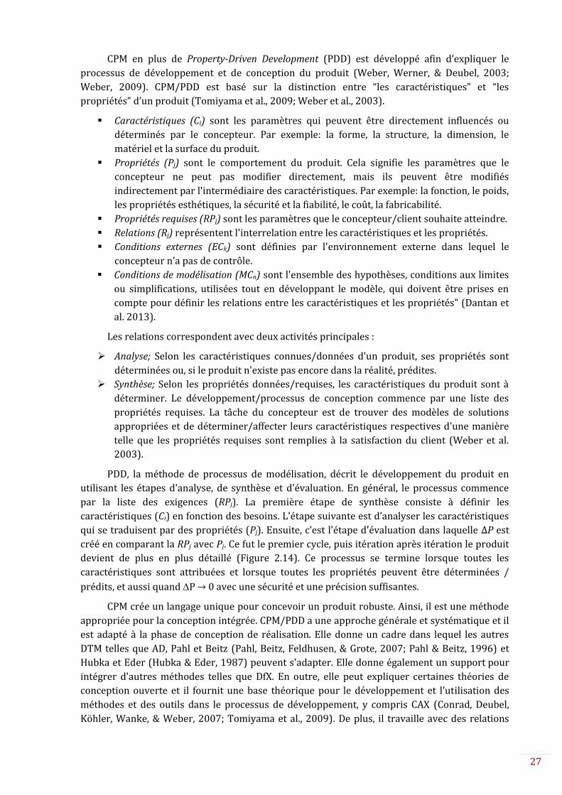
CPM en plus de Property-Driven Development (PDD) est développé afin d’expliquer le
processus de développement et de conception du produit (Weber, Werner, & Deubel, 2003;
Weber, 2009). CPM/PDD est basé sur la distinction entre “les caractéristiques” et “les
propriétés” d’un produit (Tomiyama et al., 2009; Weber et al., 2003).
Caractéristiques (Ci) sont les paramètres qui peuvent être directement influencés ou
déterminés par le concepteur. Par exemple: la forme, la structure, la dimension, le
matériel et la surface du produit.
Propriétés (Pj) sont le comportement du produit. Cela signifie les paramètres que le
concepteur ne peut pas modifier directement, mais ils peuvent être modifiés
indirectement par l'intermédiaire des caractéristiques. Par exemple: la fonction, le poids,
les propriétés esthétiques, la sécurité et la fiabilité, le coût, la fabricabilité.
Propriétés requises (RPj) sont les paramètres que le concepteur/client souhaite atteindre.
Relations (Rj) représentent l'interrelation entre les caractéristiques et les propriétés.
Conditions externes (ECk) sont définies par l'environnement externe dans lequel le
concepteur n'a pas de contrôle.
Conditions de modélisation (MCn) sont l'ensemble des hypothèses, conditions aux limites
ou simplifications, utilisées tout en développant le modèle, qui doivent être prises en
compte pour définir les relations entre les caractéristiques et les propriétés" (Dantan et
al. 2013).
Les relations correspondent avec deux activités principales :
Analyse; Selon les caractéristiques connues/données d'un produit, ses propriétés sont
déterminées ou, si le produit n'existe pas encore dans la réalité, prédites.
Synthèse; Selon les propriétés données/requises, les caractéristiques du produit sont à
déterminer. Le développement/processus de conception commence par une liste des
propriétés requises. La tâche du concepteur est de trouver des modèles de solutions
appropriées et de déterminer/affecter leurs caractéristiques respectives d'une manière
telle que les propriétés requises sont remplies à la satisfaction du client (Weber et al.
2003).
PDD, la méthode de processus de modélisation, décrit le développement du produit en
utilisant les étapes d'analyse, de synthèse et d'évaluation. En général, le processus commence
par la liste des exigences (RPj). La première étape de synthèse consiste à définir les
caractéristiques (Ci) en fonction des besoins. L'étape suivante est d’analyser les caractéristiques
qui se traduisent par des propriétés (Pj). Ensuite, c’est l'étape d'évaluation dans laquelle ∆P est
créé en comparant la RPj avec Pj. Ce fut le premier cycle, puis itération après itération le produit
devient de plus en plus détaillé (Figure 2.14). Ce processus se termine lorsque toutes les
caractéristiques sont attribuées et lorsque toutes les propriétés peuvent être déterminées /
prédits, et aussi quand P → 0 avec une sécurité et une précision suffisantes.
CPM crée un langage unique pour concevoir un produit robuste. Ainsi, il est une méthode
appropriée pour la conception intégrée. CPM/PDD a une approche générale et systématique et il
est adapté à la phase de conception de réalisation. Elle donne un cadre dans lequel les autres
DTM telles que AD, Pahl et Beitz (Pahl, Beitz, Feldhusen, & Grote, 2007; Pahl & Beitz, 1996) et
Hubka et Eder (Hubka & Eder, 1987) peuvent s'adapter. Elle donne également un support pour
intégrer d'autres méthodes telles que DfX. En outre, elle peut expliquer certaines théories de
conception ouverte et il fournit une base théorique pour le développement et l'utilisation des
méthodes et des outils dans le processus de développement, y compris CAX (Conrad, Deubel,
Köhler, Wanke, & Weber, 2007; Tomiyama et al., 2009). De plus, il travaille avec des relations

28
mathématiques et, enfin, il est adapté à des systèmes de modèle avec la complexité de la
conception.
En raison de ces avantages, il est choisi comme le cadre de l'approche proposée pour faire
face à la complexité dans IPPD. Grace à la possibilité d’intégrer des formules mathématiques
dans CPM, il crée des liens entre les modèles qualitatifs et quantitatifs. La nature des relations
dans CPM est des formules mathématiques précises, il est donc préférable à FBS.
Toutefois, le modèle de Weber (que nous appelons le CPM classique) a quelques
inconvénients lorsqu’il doit traiter la complexité dans IPPD. En outre, CPM est introduit pour la
conception de produits seulement. La nouvelle version proposée dans le chapitre 3 permettra,
nous l'espérons de réduire ces inconvenances. Dans le chapitre 6, il est expliqué comment elle
peut être utilisée pour modéliser le processus de fabrication également.

29
CHAPITRE 3 :
Proposition pour modéliser un produit
3.1. Contexte
L'objectif global de la conception est d'augmenter la valeur. Dans IPPD, les aspects de
produit et de processus sont liés respectivement à la qualité et au coût. Dans l’aspect du produit,
la difficulté est d’identifier le lien entre la fonction et la structure. De plus, l'identification du lien
est surtout qualitative, ce qui le rend difficile à utiliser dans la phase de conception détaillée.
Ainsi, un modèle quantitatif créé par la transition entre la fonction de structure est requis.
Ensuite, ce modèle peut être utilisé pour analyser le système et accroître les connaissances du
concepteur sur le système. Ainsi, le résultat peut être utilisé pour la phase de conception et de
réalisation.
Afin de créer ce modèle, une approche est nécessaire pour aider le concepteur à travers le
processus de modélisation et de conception. L'approche doit être systématique pour modéliser
un système multi-niveaux. Donc, dans ce chapitre, nous allons proposer une approche pour la
conception des produits. En plus de d'avoir cette approche hiérarchique, les deux aspects
fonction et structure doivent être assurés à chaque niveau de décomposition. Ainsi, une
approche en zigzag entre deux domaines - fonctionnel et structurel - est nécessaire. CPM est
choisi comme cadre de l'approche. Les faiblesses du CPM classique sont l'absence d'une
approche systématique et de la difficulté à identifier les relations (Rm). Par conséquent, une
version étendue du CPM est proposée dans la section suivante. Dans cette version, en plus
d’avoir plusieurs niveaux de propriétés qui sont utiles pour les systèmes complexes, elle est
systématique. Cette approche systématique est réalisée par une approche hiérarchique tout en
zigzaguant entre la fonction et la structure. L'approche d’AD est utilisée ici. Ainsi, il donne au
concepteur une approche à suivre, étape par étape. Cependant, en plus de ce cadre, nous avons
besoin d'un modèle pour assurer le lien quantitatif entre la fonction et la structure. Ce modèle
doit être basé sur le comportement du système. La réponse à ce problème est discutée dans la
section 3.3.
3.2. Une version étendue de CPM
A cause de l'absence d'une approche systématique dans la mise en œuvre de CPM, il est
compliqué de modéliser des systèmes de PDD avec plusieurs relations et propriétés. Par
conséquent, si le système est compliqué, l'identification des caractéristiques importantes au
début ne serait pas possible. Plus important, identifier les liens entre Ci et Pj n’est pas facile à
première vue. Beaucoup de liens identifiés dans le système complexe sont entre plusieurs
propriétés. Par conséquent, il y aura plusieurs niveaux de propriété. Dans ce cas, il peut y avoir
confusion dans l'identification de la prochaine étape dans la modélisation d'un produit.
A cause de ces difficultés et les faiblesses, nous avons proposé une version étendue du
CPM. Dans cette version étendue, un modèle complémentaire est utilisé, au lieu de PDD, pour
créer le modèle de système de CPM. Le modèle complémentaire crée un lien entre la fonction et

30
la structure du produit, et distingue les propriétés fonctionnelles des autres propriétés à utiliser
pour identifier les éléments et les relations dans CPM. Alors, les Pj peuvent être aux différents
niveaux. Le niveau de Pj dépend du niveau de décomposition du système ou de sa relation avec Ci
ou les autres Pj. Contrairement à PDD, notre approche proposée utilise une méthode
hiérarchique pour identifier les éléments du CPM. Donc, nous introduisons un autre élément de
CPM qui s’appelle « Propriétés intermédiaire » (IPj) :
Les propriétés intermédiaires sont des paramètres qui ne peuvent pas être classés avec des
caractéristiques ou des conditions externes, selon leurs définitions. Ils sont des propriétés, mais
diffèrent des propriétés principales (Pj). Ils sont utilisés pour décomposer le système afin de
trouver/représenter les caractéristiques liées d'une propriété dans un système complexe tout en
décomposant le système. Donc, ce sont les paramètres intermédiaires entre les propriétés
principales et les caractéristiques.
Pendant l'approche en zigzag entre deux domaines, en utilisant les paramètres identifiés
dans chaque niveau de décomposition, le CPM est construit étape par étape. Une approche
générale de la construction du modèle de produit en utilisant la version étendue du CPM est
illustré à la figure 3.4. Dans ce cas, à chaque niveau de décomposition, les propriétés du niveau
actuel sont identifiées et les paramètres effectifs sont identifiés.
Dans un système complexe, identifier les caractéristiques dans un premier temps n’est pas
toujours possible. Cette décomposition hiérarchique de la fonction désirée permet au
concepteur de décomposer le problème de conception en sous-problèmes.
Comme expliqué précédemment, une approche fonction-comportement-structure à
l'intégration des modèles quantitatifs est nécessaire pour deux phases de conceptual design et
d’embodiment design, ainsi que le lien entre eux. Donc, CPM a besoin d'un modèle
complémentaire à utiliser dans cette approche. Lutters et al. (2014) ont réunis les outils et
techniques pour la conception des produits standards. Nous sommes à la recherche d'un outil
général applicable dans les deux phases de conception, afin d'inclure les aspects fonctionnels et
structurels. Pour extraire les lois physiques afin de déterminer le modèle quantitatif, nous
proposons le modèle de flux d'énergie à utiliser dans les deux domaines fonctionnel et physique.
3.3. Modélisation de flux d’énergie (EFM)
Un flux d'énergie est un passage ou une transformation de l'énergie dans un système. Pour
modéliser les produits mécaniques, le flux d'énergie est l'un des meilleurs moyens de trouver les
liens physiques entre les éléments (Pailhès, Sallaou, & Nadeau, 2007). C’est le cas lorsque les flux
énergétiques sont les flux fonctionnels du système. Dans ce cas, le flux d'énergie peut être utilisé
pour modéliser le comportement du système et d’en déterminer les liens.
Il existe plusieurs approches de modélisation des flux d'énergie dans la littérature. Les
critères de choix de la meilleure EFM est qu'il soit être en mesure d'être intégré dans la CPM
étendue. Deuxièmement, il est nécessaire de créer un lien entre la fonction et la structure. En
troisième lieu, le modèle créé par la méthode devrait être basé sur le comportement du système.
Enfin, il aide le concepteur à identifier les paramètres efficaces.
CTOC (Convertisseur, Transmetteur, Opérateur, Contrôle) est l'un des EFMs qui est créé
par (Pailhès et al., 2007) et il peut interagir avec CPM étendue afin de satisfaire aux critères
mentionnés ci-dessus. CTOC se concentre sur structure juste nécessaire d'un système pour
répondre aux besoins. Il définit l'analyse du système selon ce cadre : l'analyse d'une fonction

31
conduit à l'identification de la circulation d’un flux fonctionnel nécessaire à la réalisation de
cette fonction. L'action est effectuée par le passage de ce flux «fonctionnel» juste nécessaire
(pour exécuter l'action demandée) qui est réalisé par la transformation et la transmission
d’énergie (Pailhès, 2013).
Donc, au lieu de considérer tous les flux, il se focalise sur les flux qui sont nécessaires pour
atteindre la fonction désirée. Puisque l'analyse est basée sur l'exigence fonctionnelle, dans la
modélisation par CTOC, la structure n’est pas nécessairement connue (comme dans Bond Graph
et IBD) mais la structure peut être construite sur la base des exigences fonctionnelles. Ainsi, il
peut être utilisé avant de connaître la description d'un système.²
Selon CTOC, un système pourrait consister de :
Convertisseur (C) : convertit l'énergie importée en énergie qui est utilisable par les autres
composants du système.
Transmetteur (T) : permet à l'énergie d'être transmise sans aucun changement dans le
type d'énergie (le type d’énergie entre l'entrée et la sortie est le même)
Opérateur (O) : permet de concrétiser l’action souhaitée au niveau de la zone opératoire.
L’opérateur peut être soit un transmetteur soit un convertisseur selon le choix de
conception retenu.
Composants de Contrôle (C) : Ils permettent d’assurer que l’action des différents
composants est correctement effectuée.
Elément de référence (R) : Il est lié au système en cours de conception (Pailhès, 2013).
Le modèle CTOC est utilisé dans notre l’approche proposée pour modéliser le
comportement du système et d'assurer la transition de la fonction à la structure. Son concept est
utilisé dans deux formes : le modèle fonctionnel et le modèle structurel. Dans le modèle
fonctionnel, l'objectif est de satisfaire aux besoins. Si le système existe ou non, la fonction peut
être divisée en plusieurs sous-fonctions. Chaque sous-fonction est définie en fonction du flux
d'énergie. Le modèle structurel, qui est basé sur le modèle fonctionnel, divise le système dans les
éléments de convertisseur, transmetteur, opérateur et contrôle. Dans ce modèle, les éléments de
référence et d'interaction doivent être précisés. L’approche systématique de la modélisation
d'un système en utilisant CTOC, AD et CPM est décrite dans la section suivante. Au dernier
niveau de décomposition, où des connaissances suffisantes sur la structure requise du système
sont obtenues / décidées, un modèle comme IBD ou Bond graph peut être utilisé pour
représenter la structure du système.
3.4. Approche proposée pour la modélisation du produit
L'approche commence par l'analyse des besoins des clients. Le besoin du client, qui a
normalement une valeur qualitative, devrait être traduit en valeur quantitative. Cette valeur
dans la terminologie de CPM est considérée comme propriété requise (RPj). Afin de quantifier les
besoins, normalement, augmenter la « valeur » est considéré comme le principal objectif. Dans
cette thèse, nous avons défini la valeur comme une grandeur pour mesurer à la fois le produit et
le processus. Donc, nous l'appelons « la valeur du produit ». Ainsi, le concepteur doit chercher les
paramètres qui sont considérés comme qualité pour le client. Ensuite, ce paramètre devient la
valeur du produit ou RPj.
L'étape suivante consiste à identifier la fonction requise pour satisfaire au(x) besoin(s).
Ainsi, le premier modèle montre l'objectif de la conception. Comme la figure 3.9 l’illustre,
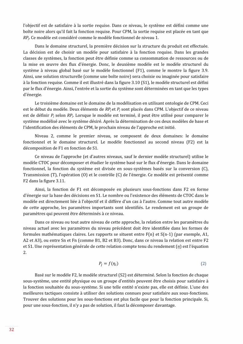
32
l'objectif est de satisfaire à la sortie requise. Dans ce niveau, le système est défini comme une
boîte noire alors qu'il fait la fonction requise. Pour CPM, la sortie requise est placée en tant que
RPj. Ce modèle est considéré comme le modèle fonctionnel de niveau 1.
Dans le domaine structurel, la première décision sur la structure du produit est effectuée.
La décision est de choisir un modèle pour satisfaire à la fonction requise. Dans les grandes
classes de systèmes, la fonction peut être définie comme sa consommation de ressources ou de
la mise en œuvre des flux d'énergie. Donc, le deuxième modèle est le modèle structurel du
système à niveau global basé sur le modèle fonctionnel (F1), comme le montre la figure 3.9.
Ainsi, une solution structurelle (comme une boîte noire) sera choisie ou imaginée pour satisfaire
à la fonction requise. Comme il est illustré dans la figure 3.10 (S1), le modèle structurel est défini
par le flux d'énergie. Ainsi, l'entrée et la sortie du système sont déterminées en tant que les types
d'énergie.
Le troisième domaine est le domaine de la modélisation en utilisant ontologie de CPM. Ceci
est le début du modèle. Deux éléments de RPj et Pj sont placés dans CPM. L'objectif de ce niveau
est de définir Pj selon RPj. Lorsque le modèle est terminé, il peut être utilisé pour comparer le
système modélisé avec le système désiré. Après la détermination de ces deux modèles de base et
l'identification des éléments de CPM, le prochain niveau de l'approche est initié.
Niveau 2, comme le premier niveau, se composent de deux domaines: le domaine
fonctionnel et le domaine structurel. Le modèle fonctionnel au second niveau (F2) est la
décomposition de F1 en fonction de S1.
Ce niveau de l'approche (et d'autres niveaux, sauf le dernier modèle structurel) utilise le
modèle CTOC pour décomposer et étudier le système basé sur le flux d'énergie. Dans le domaine
fonctionnel, la fonction du système est divisée en sous-systèmes basés sur la conversion (C),
Transmission (T), l'opération (O) et le contrôle (C) de l'énergie. Ce modèle est présenté comme
F2 dans la figure 3.11.
Ainsi, la fonction de F1 est décomposée en plusieurs sous-fonctions dans F2 en forme
d'énergie sur la base des décisions en S1. Le nombre ou l'existence des éléments de CTOC dans le
modèle est directement liée à l'objectif et il diffère d'un cas à l’autre. Comme tout autre modèle
de cette approche, les paramètres importants sont identifiés. Le rendement est un groupe de
paramètres qui peuvent être déterminés à ce niveau.
Dans ce niveau ou tout autre niveau de cette approche, la relation entre les paramètres du
niveau actuel avec les paramètres du niveau précédent doit être identifiée dans les formes de
formules mathématiques claires. Les rapports se situent entre F(n) et S(n-1) (par exemple, A1,
A2 et A3), ou entre Sn et Fn (comme B1, B2 et B3). Donc, dans ce niveau la relation est entre F2
et S1. Une représentation générale de cette relation compte tenu du rendement (η) est l'équation
2.
𝑃𝑗 = 𝑓(𝜂𝑖) (2)
Basé sur le modèle F2, le modèle structurel (S2) est déterminé. Selon la fonction de chaque
sous-système, une entité physique ou un groupe d'entités peuvent être choisis pour satisfaire à
la fonction souhaitée du sous-système. Si une telle entité n'existe pas, elle est définie. L'une des
meilleures tactiques consiste à utiliser des solutions connues pour satisfaire aux sous-fonctions.
Trouver des solutions pour les sous-fonctions est plus facile que pour la fonction principale. Si,
pour une sous-fonction, il n’y a pas de solution, il faut la décomposer davantage.

33
Comme il est illustré dans la Figure 3.11 (S2), les paramètres importants dans ce modèle
sont des propriétés intermédiaires (IPj). Bien qu'il soit rare pour un système complexe, mais il
est également possible d'identifier les caractéristiques (Ci). L'équation générale est que
l'équation 3.
𝜂𝑖 = 𝑓(𝐼𝑃𝑗) (3)
Attribuer/définir les composants dans CTOC commence par l’Opérateur (O) comme
l’élément principale. Puis, selon des types d'énergie reçus, si le Transmetteur (T) et/ou le
convertisseur (C) sont nécessaires, ils seront ajoutés. A part ces éléments, si une entité est
responsable de contrôler le fonctionnement des autres composants, elle est nommé contrôle (C).
Cette tactique CTOC est applicable dans les deux domaines fonctionnels et structurels.
Comme il est indiqué, dans la loi de TRIZ, le concepteur devrait se concentrer sur les
exigences juste nécessaires pour décrire le système. Donc, dans la modélisation du système basé
sur CTOC, divisant le système dans les éléments, ne signifie pas nécessairement avoir tous les
éléments de C, T, O et C. En fait, le concepteur doit essayer d'atteindre un système idéal, avec un
minimum d'éléments nécessaires. Avec cette approche, la complexité du système sera ainsi
réduite.
Cette approche en zigzag entre les domaines fonctionnel et structurel continue jusqu’à ce
que le système se décompose encore plus. Le nombre de niveaux de décomposition dépend de la
complication du système et de l'objectif du concepteur, de ce qu'il cherche et de quel niveau de
détail il a besoin.
Le dernier niveau est le niveau structurel détaillé (toujours au stade précoce de la
conception). Avec les connaissances acquises sur les entités minimales requises à partir du
modèle de flux d'énergie, le concepteur a une base pour la conception du produit. Pour le modèle
structurel dans ce niveau (Sn), « Diagramme bloc », qui est l'un des schémas de System Modelling
Language (SysML) (Friedenthal, Moore, & Steiner, 2012) qui peuvent être utilisés. Bien que tous
les types de relations (comme physique, signal, ...) peuvent être utilisés dans le diagramme bloc,
l'accent est mis sur le flux d'énergie qui est étudié dans le niveau précédent. En outre, d'autres
liens tels que des références doivent être maintenues aussi bien.
Les paramètres importants, en fonction de l'objectif, sont identifiés. Si l'on considère
qu'aucune autre décomposition n’est nécessaire, cela signifie que les paramètres de ce niveau
sont tous Ci. Un modèle complet signifie l'identification de tous les paramètres efficaces et leurs
relations. Une représentation générale de ce modèle est illustrée à la figure 3.12.
A partir de paramètres déterminés dans chaque modèle, les impacts environnementaux
doivent être pris en compte. Ces paramètres sont notés en tant que ECk dans les formules. Donc ;
𝑃𝑗 = 𝑓(𝐶𝑖, 𝐼𝑃𝑗, 𝐸𝐶𝑘) (4)
Dans chaque modèle, il y a des suppositions, des hypothèses et des simplifications qu’il
faut considérer dans le processus de la modélisation. Selon la définition, ils sont les conditions
de modélisations (MCn) dans CPM. De ce fait, dans chaque relation (Rm) il pourrait y avoir un ou
plusieurs MCn. Donc, l’équation finale qui est le résultat de l’approche est comme l’équation 5.
𝑃𝑗 = 𝑓(𝐶𝑖, 𝐸𝐶𝑘|𝑀𝐶𝑛) (5)

34
La détermination de modèle et l’identification des fonctions et des paramètres sont la
phase 1. La phase 2 est d’utiliser ce modèle pour analyser le comportement du système. Donc,
les impacts de Ci et ECk sur la sortie du système peuvent être analysés.
Ainsi, par l'équation 5, le concepteur peut modifier les principales propriétés (Pj) en
modifiant les caractéristiques (Ci). La modification de Ci se traduira par des changements d’IPj.
Les changements dans chaque niveau affecteront des changements de niveau supérieur. Ce
processus se poursuivra jusqu'à ce que les Pj soient obtenues. Les modifications sont en rapport
avec la comparaison entre Pj et RPj. Après avoir analysé l'effet des caractéristiques sur les
propriétés principales, le concepteur aura des idées sur l'amélioration du produit. La direction
de cette amélioration est de minimiser l'écart entre Pj et RPj (ΔPj → 0). L'analyse de sensibilité est
faite dans le chapitre 5.
L'exploitation du modèle obtenu pour l'analyse de sensibilité, l'optimisation et l’élicitation
de l'incertitude seront présentés dans les chapitres 5 et 6. Le même cadre va être utilisé pour
modéliser un système dans la conception intégrée, comme décrit dans le chapitre 5.
La proposition de ce chapitre est également publiée dans (Malmiry, Dantan, Pailhès, &
Antoine, 2016a).

35
CHAPITRE 4 :
Étude de cas : L’approche de modélisation du
produit
4.1. Pompe à l’huile
Les pompes sont des dispositifs utilisés pour générer des flux et transmettre des fluides. Il
existe différents types de pompes caractérisées par sa cylindrée, le niveau de pression supporté,
le rendement, etc. La pompe qui est utilisé comme étude de cas est la pompe à engrenages
externes qui est utilisé dans une automobile Renault®. Cette pompe utilise deux pignons qui
tournent en sens inverse pour délivrer l'huile. Les pompes à engrenages externes ont des
tolérances serrées et comportent des arbres-supports de part et d’autres des pignons. Un
modèle 3D de celui-ci est illustré sur la figure 4.4
4.2. Modélisation du produit
Dans cette section, l’implémentation de l'approche proposée sur cette étude de cas est
présentée. La fonction principale est d’envoyer l’huile et la sortie requise est « le débit requis »
(RQ). L'entrée est l'énergie mécanique et le fonctionnement du système peut être défini comme
la transformation de l'énergie mécanique en énergie hydraulique. La sortie requise est imposée
par le fabricant d'avoir un flux d'au moins 5,46 × 10⁻⁴ m3/s au régime minimum pour une voiture
en état de repos pour avoir un débit suffisant pour la lubrification des pièces. Ainsi, le premier
niveau de l'approche est comme illustré à la Figure 4.5.
Au deuxième niveau, le fonctionnement du système est divisé en sous-systèmes sur la base
des éléments de CTOC. La sous-fonction principale est de « générer de l'énergie hydraulique ».
L'entrée est l'énergie mécanique. Cependant, un élément de Transmetteur est nécessaire pour
transmettre l'énergie reçue du moteur à la zone d'opération. En outre, l'élément de contrôle est
nécessaire pour assurer la pression du débit d'huile de sortie. Le rendement hydromécanique
(ηhm) et le rendement volumétrique (ηv) sont les IPj. Ces paramètres (ηv, ηhm) sont placés dans le
modèle.
Afin d'obtenir la première équation, les phénomènes physiques dans la pompe à huile et
son environnement doivent être étudiés. L'entrée comprend deux paramètres M (couple) et ω
(vitesse de rotation angulaire). Ces deux paramètres en plus de Δp (l'augmentation de pression)
sont des ECk. Par conséquent, R1 est obtenue en tant que première équation pour déterminer les
paramètres effectifs de Q.
𝑄 =
𝑀.𝜔
∆𝑝× 𝜂𝑣 . 𝜂ℎ𝑚 (𝑅1) (6)
Selon le modèle fonctionnel à la figure 4.6(a), les décisions nécessaires sont prises et le
modèle structurel est créé. Ce modèle est illustré sur la figure 4.8(a). Le paramètre important
dans la transmission de l'énergie mécanique (T) est le couple de frottement (MF). En plus de MF,

36
la cylindrée (V) et la pression (Δp) sont également liés à ηhm en considérant le couple théorique
(M). Donc, le rendement peut être calculé comme l’équation 7. Egalement, la formule pour
calculer ηv en utilisant la perte de charge (Ql) est comme l’équation 8.
𝜂ℎ𝑚 =
𝑉
2𝜋. (𝑀 −𝑀𝐹)∆𝑝 (𝑅2) (7)
𝜂𝑣 = 1 −
2𝜋. 𝑄𝑙𝑉.𝜔
(𝑅3) (8)
MC1, comme il est indiqué dans la figure 4.8, est la simplification dans l’équation R2. Dans
cette équation, seulement l’effet de couple de frottement est pris en compte. En plus, cet effet est
limité aux frottements dans les paliers et des dents d'engrenage. Les simplifications et les
hypothèses similaires sont considérées dans les autres relations comme ils sont notés en tant
que MCn.
Pour analyse des détails, deux paramètres de V et Ql ont besoin une étude plus
approfondie. V peut être estimé avec l’équation 9.
𝑉 ≈ 2.25 × 𝜋 ×ɱ2 × 𝑍 × 𝐿𝐺 (𝑅6) (9)
La perte de charge est divisée en trois parties: La fuite radiale (Qlr), les fuites axiales (Qlab
et Qlat).
𝑄𝑙 = 𝑄𝑙𝑟 +𝑄𝑙𝑎𝑡 + 𝑄𝑙𝑎𝑏 (𝑅4) (10)
Comme c’est illustré dans les équations 11, 12 et 13, les fuites internes peuvent être
calculées selon les jeux qui sont liés aux tolérances.
𝑄𝑙𝑟 = 2 ×𝐿𝐺ℎ𝑟̅̅ ̅
3
8𝜇 × (𝑍 − 3)𝑙ℎ∆𝑝̅̅̅̅ (𝑅7) (11)
𝑄𝑙𝑎𝑡 =𝐻
8𝜇 × √𝑙ℎ . 𝑙𝑝. 𝑙𝑏3
(ℎ𝑎̅̅ ̅2⁄ )
3
. (2
3+
4
𝑍 − 3)∆𝑝̅̅̅̅ (𝑅8) (12)
𝑄𝑙𝑎𝑏 = 4 ×
2𝜋 (ℎ𝑎̅̅ ̅2⁄ )
3
8𝜇. ln (𝐷𝑟𝐷𝑠⁄ )
∆𝑝 (𝑅9) (13)
La figure 4.11 illustre les jeux accompagnés par les dimensions géométriques connexes. La
liste de ces paramètres, en plus de tous les autres paramètres de cette étude de cas, est
rassemblée dans le tableau en annexe A.
Dans les relations R7, R8 et R9, tous les paramètres sont Ci sauf les jeux (ha et hr). Donc, les
équations 14 et 15 sont utilisées pour avoir les rapports aux dimensions géométriques.
ℎ𝑟̅̅ ̅ =
𝑀𝑖𝑛(𝐷𝑐) − 𝑀𝑎𝑥(𝐷𝐺 + 𝐴𝑥)
2 (𝑅12) (14)
ℎ𝑎̅̅ ̅ = 𝑀𝑖𝑛(𝐿𝐶) − 𝑀𝑎𝑥(𝐿𝐺) (𝑅13) (15)

37
En outre, le couple de frottement dans l’équation 7 doit être décomposé. Ainsi, les
formules suivantes sont obtenues selon les phénomènes physiques, les besoins, et les
caractéristiques de la pompe.
𝑀𝐹 = 𝑀𝐹1 +𝑀𝐹2 (𝑅5) (16)
𝑀𝐹1 = (𝜇. 𝐷𝑠. 𝜔.𝐿𝑠2) × (ℎ𝑏 (
4𝜋(1 + 2𝑛2)
(3 − 𝑛2)√𝑛2)) × (
𝐷𝑠2)2
(𝑅11) (17)
Quand;
𝑛 = √𝐾
√1+𝐾 , et 𝐾 =
−(1−3𝐵2)+((1−3𝐵2)2+8𝐵2)
0.5
2, et 𝐵 =
𝐹
12𝜋.𝜇.𝜔.𝐷𝑠2.𝐿𝑠× (
2ℎ𝑏
𝐷𝑠)2
Et;
𝑀𝐹2 = 𝜇. (𝐷𝐺2)2
.𝜔. 𝐿𝐺ℎ𝑟
.
(
4𝜋(1 + 2𝑛𝐺
2)
(𝑛𝐺2 + 2).√1 − 𝑛𝐺
2
)
× 10−6 ×𝐷𝐺2 (𝑅10) (18)
Encore, le jeu hb peut être écrit selon les dimensions géométriques:
ℎ𝑏 =
𝐷𝑏 − 𝐷𝑠2
(𝑅14) (19)
Maintenant que toutes les caractéristiques requises (Ci) et les conditions externes (ECk)
sont identifiées, la représentation de CPM du modèle est terminée. Ce modèle est représenté en
partie CPM de la figure 4.12. Sur cette figure, tous les Ci se trouvent dans la colonne de droite.
Ainsi, avec la première vue sur ce modèle, on peut voir tous les paramètres modifiables efficaces
du système. Avec le modèle créé et identifié tous les relations entre les paramètres, l'équation
suivante est obtenue:
𝑃𝑗 = 𝑓(𝐶𝑖, 𝐸𝐶𝑘|𝑀𝐶𝑛) ⇒𝑄
= 𝑓(𝑚, 𝑍, 𝑙ℎ , 𝑙𝑝, 𝑙𝑏 , 𝐿𝐺 , 𝐷𝐶 , 𝐷𝐺 , 𝐿𝐶 , 𝐻, 𝐷𝑟, 𝐷𝑠, 𝐷𝑏, 𝐿𝑠, 𝑀, 𝜔, ∆𝑝, 𝜇 | 𝑀𝐶1,𝑀𝐶2,𝑀𝐶3,𝑀𝐶4,𝑀𝐶5) (20)
Grace à cette équation, l’impact de chaque Ci ou ECk ou de leur combinaison sur Q ou sur
n’importe quelle IPj peut être analysé en utilisant l’analyse de sensibilité locale. De plus, dans un
analyse de sensibilité globale (Saltelli et al., 2008), l’importance de chaque paramètre peut être
évalué. Ces analyses peuvent être utilisées pour optimiser un produit existant ou pour concevoir
un nouveau produit hautes performances. L’analyse de sensibilité de cette étude de cas est
présentée dans le chapitre 5 et l’optimisation sera présentée dans le chapitre 6.
4.3. Les outils complémentaires
Tout en suivant l'approche proposée, selon le cas, le concepteur peut utiliser des outils
complémentaires. Le but est d'extraire suffisamment d'informations dans chaque niveau de
l'approche afin de déterminer chaque modèle (F1, F2, ... S1, S2, ...).
L'analyse fonctionnelle est l'un des outils qui peuvent être utilisés pendant l'approche.
L'analyse fonctionnelle est un outil pour évaluer la satisfaction de la clientèle qui, dans notre cas,
signifie la fonctionnalité du produit. Au moyen de cet outil, on identifie les fonctions du produit à

38
évaluer. En outre, elle montre les relations entre les composants du produit, ainsi que entre le
produit et les autres composants du système, en termes de fonctionnalité. Dans un niveau plus
profond de l'étude, l'analyse de la fonction nous donne les liaisons entre les entités qui peuvent
être poursuivies pour la conception structurelle.
Afin d'illustrer la fonction du produit et de sa relation avec d'autres composants, «
Diagramme Pieuvre » est utilisé. Ce schéma est utilisé pour analyser les besoins et identifier les
fonctions d'un produit.
Pour identifier les relations entre les caractéristiques avec les fonctions, le Tableau
d’Analyse Fonctionnelle Technique (TAFT) est utilisé. Cet outil qui est proposé par Charpentier &
Mathieu (2000) capitalise toutes les informations requises pour la spécification fonctionnelle
des composants. L’analyse géométrique des besoins fonctionnels du produit est l'étape-clé pour
l'amélioration de la conception du produit (Charpentier & Mathieu, 2000). Ce tableau analyse
chaque entité du système en ce qui concerne l'action liée vers la satisfaction de la fonction
requise du système. Cet outil n’est pas nécessaire pour initier la démarche proposée. Utiliser cet
outil est possible si la structure du système est connue. Une version étendue de cette table sera
utilisée comme une étude primaire pour étudier le processus de fabrication de la pompe à huile
dans le chapitre 5.
Dans le chapitre suivant, on montre comment cette approche peut être utilisée pour la
gestion de l'incertitude et de la gestion de la complexité. Le prochain chapitre se concentrera
également sur la phase 2 de l'approche pour analyser le système basé sur le modèle déterminé à
identifier les principales caractéristiques. Le chapitre 6 est une extension de cette approche qui
peut être utilisé pour modéliser le système de fabrication dans un environnement de conception
intégré produits et processus. La même étude de cas qui est étudié dans ce chapitre sera utilisée.
La différence est que, dans chaque niveau de décomposition, les décisions sont prises en
impliquant le facteur de coût aussi.

39
CHAPITRE 5 :
Gestion de l’incertitude et la complexité
dans la conception de produit
5.1. Gestion de l’incertitude
La première section de ce chapitre explique comment l'approche proposée peut aider le
concepteur à gérer l'incertitude dans le processus de conception. L'exploitation de l'approche
afin de gérer l'incertitude comprend deux aspects. Le premier aspect est de savoir comment
utiliser l'approche pour l’élicitation de l'incertitude dans le processus de conception qui est une
exigence principale pour la gestion de l'incertitude. Le deuxième aspect utilise l'approche pour
la gestion de l'incertitude épistémique et donc de réduire la complexité de conception qui est à
cause de ce type d'incertitude.
Différents types d'incertitude existent dans toutes les étapes du processus de conception.
Considérant les quatre phases de la conception, l'incertitude doit être identifiée et gérée dans
chaque phase :
1) Planification et clarification des tâches: Dans cette phase, il y a toujours l'incertitude
épistémique dans la précision des informations recueillies sur les exigences et les
contraintes.
2) Conceptual design: Dans cette phase la solution possible au problème de conception est
déterminée. l'incertitude épistémique dans les décisions du concepteur vers
l'identification d'une solution est inévitable.
3) Embodiment design: Le concept obtenu dans la phase précédente est concrétisé et
détaillé dans cette phase. Il existe différents types d'incertitude épistémique dans les
décisions prises, les facteurs efficaces identifiés, des critères déterminés et le
comportement du système.
4) La conception détaillée: Dans cette phase, la conception détaillée, y compris les formes,
les surfaces, les tolérances et les matériaux, est construite en fonction de la conception
de la phase précédente. En plus de l'incertitude épistémique en raison des décisions de
cette phase ou des phases précédentes, l'existence d'une incertitude aléatoire de la
valeur des entités physiques et les impacts environnementaux sont inévitables.
Donc, il y a différents types d'incertitude à identifier et à gérer dans le processus de
modélisation et de conception. Par conséquent, nous devons d'abord classer les types
d'incertitude dans notre domaine. Nous avons classifié l’incertitude dans la conception selon la
taxonomie classique et (Thunnissen, 2005). On divise l'incertitude en aléatoire et épistémique.
L’incertitude épistémique est divisée en cinq sous-catégories : l'incertitude du modèle,
l'incertitude phénoménologique, l’incertitude comportementale, l'ambiguïté et l'interaction.
Afin de gérer l'incertitude, il y a deux approches principales. La première approche
consiste à réduire l'incertitude elle-même. Cette réduction est possible lorsqu’unegrande
quantité de données est disponible ou lorsque le concepteur a une connaissance assez complète

40
du système. La conception d'un nouveau produit ayant ce genre de connaissances n’est pas
possible. Cela souligne l'importance de la « conception robuste » comme la deuxième approche.
Dans la conception robuste, il existe trois types d'informations: les facteurs de contrôle, les
facteurs de bruit et les réponses. Les facteurs de contrôle ou les paramètres de conception sont
les paramètres que le concepteur peut ajuster. Ceci est similaire aux caractéristiques (Ci) dans
l’ontologie de CPM. Les facteurs de bruit sont l'impact environnemental sur un système que le
concepteur ne peut pas contrôler. Dans CPM, ces paramètres sont appelés les conditions
externes (ECk). Enfin, les réponses sont la sortie d'un système ou les propriétés (Pj) dans CPM.
Ces types d'information sont représentés sur la figure 5.2.
Il y a trois aspects dans l'approche qui peuvent être utilisés pour réduire l'incertitude
épistémique :
1. L'incertitude dans l'identification des fonctions, la structure et le comportement requis du
système
L'approche proposée commence par identification du RPj. D'après le RPj, la fonction
requise du système est définie ou identifiée. Le flux d'énergie modèle le comportement du
système en utilisant CTOC. De plus, dans chaque niveau de décomposition dans l'approche
proposée, la fonction du système ou du sous-système est analysée. Le modèle de flux d'énergie
dans chaque niveau de décomposition (les domaines fonctionnel et structurel), qui maintient la
cohérence entre les modèles et la fonction du système, peut être décomposé jusqu’à la structure.
Ainsi, il établit un lien entre la fonction et la structure. Subséquemment, il peut accroître les
connaissances du concepteur vers le comportement du système, et la relation de la structure
avec la fonction qui doit être satisfaite.
2. L'incertitude dans l'identification des paramètres effectifs
A chaque niveau de l'approche, grâce au flux d'énergie, les paramètres importants sont
identifiés. L'importance de ces paramètres est basée sur l'objectif de concepteur et sur la
fonction du système ou sous-systèmes. Ces éléments sont établis en tant que les propriétés
requises (RPj), les propriétés (Pj), ou les propriétés intermédiaires (IPj) de CPM. Un autre groupe
de paramètres dans CPM est la condition externe (ECk). Si le concepteur estime qu'il y a des
impacts environnementaux sur la fonction du système, ils peuvent être ajoutés. Ainsi, l'effet créé
dans le modèle peut être évalué par l'équation du modèle de résultat. En outre, cette approche
donne une piste pour le concepteur pour chercher ces paramètres. Dans chaque transition de
fonction à la structure, ou d'un niveau à l'autre, les relations (Rij) doivent être déterminées.
Normalement, cela se fait à l'aide d'équations d'énergie comme cela a été expliqué dans le
chapitre 3. Si d'autres paramètres sont apparus dans l'équation et ne peuvent pas être classés
comme Ci ou Pj, ils doivent être considérés comme ECk.
3. L’incertitude dans les relations entre les paramètres de la conception
L'approche proposée crée une piste pour le concepteur pour la décomposition
fonctionnelle. A chaque niveau de décomposition, dans les deux domaines fonctionnel et
structurel, les paramètres importants, ainsi que la relation entre eux ont été identifiés.
L'identification des équations est basée sur les phénomènes physiques. L'approche proposée
décompose le problème de conception, il est donc plus facile à gérer. L'étude systématique étape
par étape du système rend les identifications des phénomènes physiques plus faciles et on peut
donc atteindre les relations.
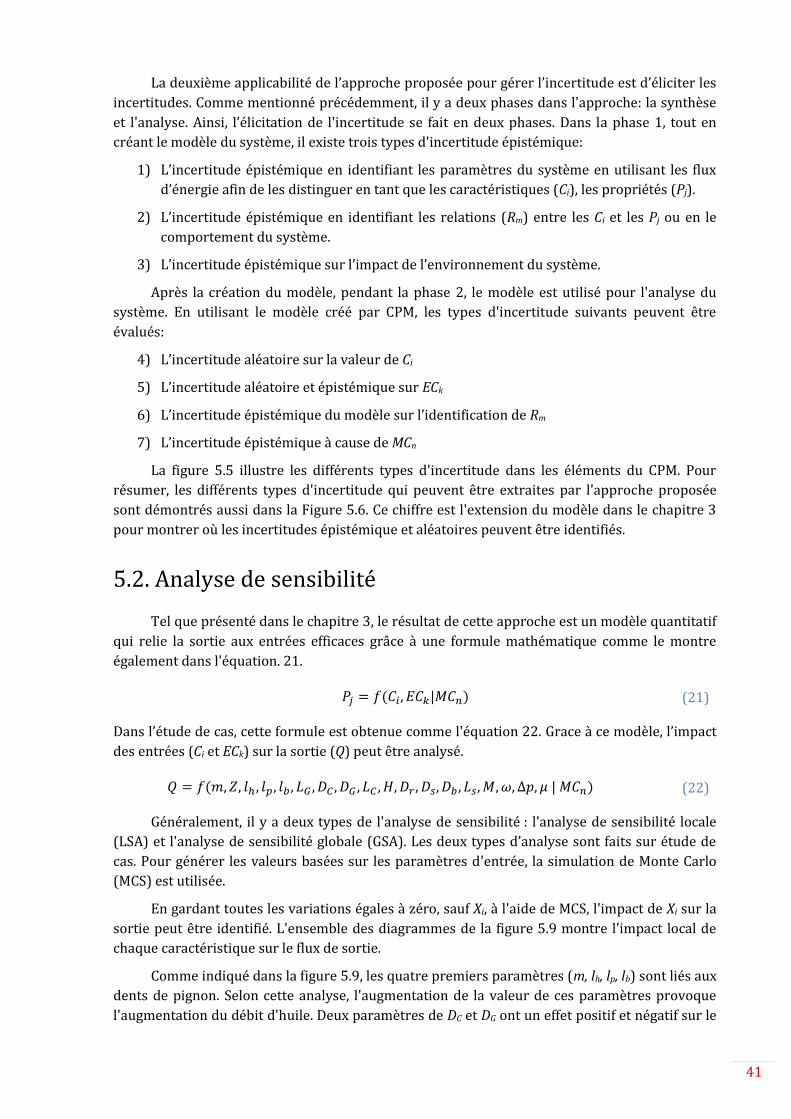
41
La deuxième applicabilité de l’approche proposée pour gérer l’incertitude est d’éliciter les
incertitudes. Comme mentionné précédemment, il y a deux phases dans l'approche: la synthèse
et l'analyse. Ainsi, l’élicitation de l'incertitude se fait en deux phases. Dans la phase 1, tout en
créant le modèle du système, il existe trois types d'incertitude épistémique:
1) L’incertitude épistémique en identifiant les paramètres du système en utilisant les flux
d’énergie afin de les distinguer en tant que les caractéristiques (Ci), les propriétés (Pj).
2) L’incertitude épistémique en identifiant les relations (Rm) entre les Ci et les Pj ou en le
comportement du système.
3) L’incertitude épistémique sur l’impact de l’environnement du système.
Après la création du modèle, pendant la phase 2, le modèle est utilisé pour l'analyse du
système. En utilisant le modèle créé par CPM, les types d'incertitude suivants peuvent être
évalués:
4) L’incertitude aléatoire sur la valeur de Ci
5) L’incertitude aléatoire et épistémique sur ECk
6) L’incertitude épistémique du modèle sur l’identification de Rm
7) L’incertitude épistémique à cause de MCn
La figure 5.5 illustre les différents types d'incertitude dans les éléments du CPM. Pour
résumer, les différents types d'incertitude qui peuvent être extraites par l'approche proposée
sont démontrés aussi dans la Figure 5.6. Ce chiffre est l'extension du modèle dans le chapitre 3
pour montrer où les incertitudes épistémique et aléatoires peuvent être identifiés.
5.2. Analyse de sensibilité
Tel que présenté dans le chapitre 3, le résultat de cette approche est un modèle quantitatif
qui relie la sortie aux entrées efficaces grâce à une formule mathématique comme le montre
également dans l'équation. 21.
𝑃𝑗 = 𝑓(𝐶𝑖, 𝐸𝐶𝑘|𝑀𝐶𝑛) (21)
Dans l’étude de cas, cette formule est obtenue comme l'équation 22. Grace à ce modèle, l’impact
des entrées (Ci et ECk) sur la sortie (Q) peut être analysé.
𝑄 = 𝑓(𝑚, 𝑍, 𝑙ℎ , 𝑙𝑝, 𝑙𝑏 , 𝐿𝐺 , 𝐷𝐶 , 𝐷𝐺 , 𝐿𝐶 , 𝐻, 𝐷𝑟, 𝐷𝑠, 𝐷𝑏 , 𝐿𝑠, 𝑀, 𝜔, ∆𝑝, 𝜇 | 𝑀𝐶𝑛) (22)
Généralement, il y a deux types de l'analyse de sensibilité : l’analyse de sensibilité locale
(LSA) et l'analyse de sensibilité globale (GSA). Les deux types d’analyse sont faits sur étude de
cas. Pour générer les valeurs basées sur les paramètres d'entrée, la simulation de Monte Carlo
(MCS) est utilisée.
En gardant toutes les variations égales à zéro, sauf Xi, à l'aide de MCS, l'impact de Xi sur la
sortie peut être identifié. L'ensemble des diagrammes de la figure 5.9 montre l'impact local de
chaque caractéristique sur le flux de sortie.
Comme indiqué dans la figure 5.9, les quatre premiers paramètres (m, lh, lp, lb) sont liés aux
dents de pignon. Selon cette analyse, l'augmentation de la valeur de ces paramètres provoque
l'augmentation du débit d'huile. Deux paramètres de DC et DG ont un effet positif et négatif sur le

42
flux respectivement. La différence de ces paramètres est le jeu radial (hr). Deux paramètres de LC
et LG sont liés au jeu axial (ha). Donc, comme cette analyse confirme, diminuer les jeux aboutira
l'augmentation Q. De la même manière, (Dr - Ds) est le jeu du palier et la diminution de cette
valeur aboutira l'augmentation de Q. Les quatre derniers paramètres de la figure 5.9 montrent
l'impact des conditions externes sur le flux.
La seconde analyse de sensibilité locale est la variation des sorties en fonction de la
variation efficace des entrées. Comme l'équation 23 montre, l'impact de la variation des
caractéristiques et des conditions externes sur le débit (Q) et sur le rendement total (ηt) peut
être calculé.
𝐿𝑆𝐴𝑖 =𝜎𝑝𝑒𝑟𝑓𝑜𝑟𝑚𝑎𝑐𝑒 𝑖
𝜎𝑇𝑜𝑡𝑎𝑙 𝑝𝑒𝑟𝑓𝑜𝑟𝑚𝑎𝑛𝑐𝑒
→𝜎𝐶𝑖𝜎𝑄 ,𝜎𝐶𝑖𝜎𝜂 ,𝜎𝐸𝐶𝑘𝜎𝑄
,𝜎𝐸𝐶𝑘𝜎𝜂
(23)
Le tableau 5.3 est le résultat de cette analyse pour déterminer l'impact de Ci et ECk sur le
débit et le rendement. Par conséquent, la variation de « m » implique la plus grande variation sur
les sorties. Après cela, parmi les caractéristiques, celles qui sont liées aux jeux et la perte de
charge, ont l'effet le plus élevé. Parmi les conditions extérieures, c’est la vitesse angulaire (ω) qui
modifie le plus Q et la variation de la montée en pression (Δp) a le plus grand impact sur le
rendement.
L’analyse suivante est le changement de la valeur moyenne des caractéristiques et
l’analyser de l’impact de ce changement sur la sortie (l’équation 24). Le résultat est dans le
tableau 5.5.
𝐿𝑆𝐴𝑖 =
𝑃𝑒𝑟𝑓𝑜𝑟𝑚𝑎𝑛𝑐𝑒ℎ𝑖+𝑘 − 𝑃𝑒𝑟𝑓𝑜𝑟𝑚𝑎𝑛𝑐𝑒ℎ𝑖−𝑘ℎ𝑖+𝑘−ℎ𝑖+𝑘
(24)
La seconde analyse de sensibilité est l’analyse de sensibilité globale. En utilisant la boîte à
outil de FERUM® 4.1, l’indice de Sobol a été évalué au moyen d’uneprocédure d'échantillonnage
de Quasi-Monte Carlo (QMC). Le résultat de cette analyse illustre l'importance de l’impact de
chaque paramètre sur la sortie. Par ailleurs, l'importance de l'effet de la combinaison des
paramètres est analysée aussi. Considérant 15 paramètres (11 Ci et 4 ECk), il y aura 2^15
résultats. Donc, dans ce rapport, seulement une partie du résultat est présentée.
Le tableau 5.6 présente les résultats du premier indice et l'indice total des 15 paramètres.
Comme il est représenté, m et ω ont l'impact le plus élevé sur Q parmi les Ci et les ECk
respectivement. Ce résultat est en concordance avec le résultat de la LSA.
Pour analyser l'impact de la combinaison des paramètres sur la sortie, les quatre
paramètres, DC, DG, LC, LG, parmi les caractéristiques et les quatre paramètres de conditions
externes sont choisies. Les quatre caractéristiques choisies sont liées aux jeux radiaux et axiaux.
Le tableau 5.7 montre l'impact de la combinaison de ces caractéristiques. En outre, d'après le
tableau 5.6, LG est le paramètre le plus influent parmi les quatre paramètres. Cependant,
l'importance de la combinaison des deux par deux ou trois par trois d'entre eux est à peu près la
même. Selon le résultat du tableau 5.6, ω a l'impact le plus élevé. De plus, la combinaison des
paramètres ont le même niveau d'effet sur la sortie. Le tableau 5.8 est l'analyse de sensibilité
globale des conditions externes sur la sortie pour déterminer l'importance des paramètres ou
des combinaisons d'entre eux.

43
5.3. Analyse de tolérance
La troisième section de ce chapitre explique comment l'approche et le résultat obtenu
peuvent donner une piste au concepteur pour analyser la tolérance. En fait, l'applicabilité de
l'approche dans l'analyse de la tolérance est une extension de son applicabilité dans l'analyse de
sensibilité, qui a été expliquée dans la section précédente.
Le resserrement des tolérances conduit à l’augmentation de la qualité et du coût. Certains
fabricants préfèrent avoir un faible coût de fabrication, même si le résultat n’est pas un produit
haut de gamme. Bien que, d'autres fabricants préfèreront de meilleurs produits, même si ils
doivent en augmentent le coût et donc le prix. Ainsi, un compromis doit être atteint entre ces
deux axes. Cependant, la question est la même pour tous: « Est-ce que le niveau de qualité vaut
son coût? ».
Pour répondre à cette question, l'approche pour modéliser un système dans la conception
intégrée sera présentée dans le chapitre 6. Dans ce chapitre, l'aspect qualité des tolérances est
focalisé. Grace à l'approche proposée, EFM-CPM crée un lien entre la qualité et la structure, et
donc entre la performance et les tolérances.
Le concepteur doit d'abord trouver le lien entre la fonction de système et de ses
spécifications. D'autre part, l’impact des tolérances associées à chaque spécification sur la
performance du système est analysé. La difficulté est de lier les exigences fonctionnelles
qualitatives aux tolérances fonctionnelles quantitatives. Ainsi, une approche multi-physique est
nécessaire pour assurer la transition de la fonction des tolérances en tenant compte à la fois des
aspects qualitatifs et quantitatifs.
L'approche proposée crée un lien quantitatif entre la performance fonctionnelle et les
tolérances fonctionnelles. Donc, dans cette section, il sera expliqué, comment la deuxième phase
de l'approche peut être utilisée dans l'analyse de la tolérance et comment l'intégration de
tolérancement dans l'approche proposée peut aider le concepteur dans la gestion de
l'incertitude et la réduction de la complexité.
Comme dans l’analyse de sensibilité, le résultat de la phase de modélisation, (l'équation
5.2) est appliqué pour l'analyse de la tolérance. Comme illustré dans la section 5.2, grâce à cette
équation, qui est la combinaison des relations dans CPM, on peut évaluer l'impact des
caractéristiques et des conditions externes sur la performance du système. Un groupe important
de caractéristiques de CPM est des dimensions géométriques de pièces. Ces dimensions sont le
résultat de processus de fabrication. Ainsi, selon la précision du processus de fabrication, des
intervalles de tolérances différentes peuvent être assignées à chaque Ci, comme indiqué dans
l'équation 25.
𝑃𝑗 = 𝑓(𝐶𝑖) 𝑤ℎ𝑒𝑟𝑒 𝑔(𝐶𝑖) ≤ 𝑇𝐼𝑖 (25)
Au point de vue du tolérancement, une précision inférieure au processus conduira à plus
d'intervalle entre deux paramètres de tolérance. Une tolérance intervalle supérieure signifie
qu’il y a plus de chances d'obtenir un produit avec perte de charge plus élevée qu’acceptable.
Donc, il y a plus de probabilité d’avoir un produit de faible qualité.
L’équation 21 contient également l'effet des conditions extérieures (ECk) sur la sortie du
système. Contrairement à Ci, la variation d’ECk est principalement pendant le fonctionnement du
système. Ainsi, il fait partie du comportement du système. En comparaison avec les Ci, la valeur

44
de ces paramètres varie dans un intervalle plus grand. Donc, l'analyse ECk en phase 2 est
importante pour assurer le bon fonctionnement du système dans différentes conditions
environnementales.
La seconde application de l'approche en tolérancement est liée à la condition de
modélisation (MCn). Toutes les analyses en phase 2 dépendent des conditions de modélisation
qui ont été définies par le concepteur en phase de modélisation. Donc, il est important d'analyser
la probabilité de respecter MCn, ainsi que l'impact de MCn sur la performance du modèle du
système.
MCn est pour simplifier le processus de modélisation ou de se concentrer sur l'objectif de
la modélisation. Cependant, il est important de ne pas tenir compte des conditions qui
provoquent l'élimination d'un aspect important du système. En utilisant l'équation 26 et 27, les
conditions de modélisation doivent être vérifiées.
𝑃𝑟𝑜𝑏𝑎. (𝑀𝐶𝑛) ≥ 𝑋 (26)
𝑃𝑟𝑜𝑏𝑎. [𝑓(𝐶𝑖, 𝐸𝐶𝑘) ≥ 𝑌|𝑀𝐶𝑛] (27)
L’équation 26 calcule la probabilité de respecter MCn. Donc X est lié à la probabilité de
l'hypothèse. L’équation 27 est la probabilité d'avoir les performances requises tout en
respectant la MCn. Par conséquent, Y est lié à l'impact de l'hypothèse sur les performances du
système. X et Y dans l'équation 26 et 27 sont définies par le client et/ou le concepteur. L'un des
exemples de la condition de la modélisation dans l’étude de cas discutée est:
MC1: « Il n'y a pas de frottement entre les dents des engrenages et le carter. »
Cette déclaration signifie d'abord, le jeu entre les engrenages et le carter devant être
supérieure à zéro pour faire l'assemblage possible. Un jeu négatif (DC < DG) pourrait se produire
après la fabrication des composants et avant l'assemblage.
Deuxièmement, le jeu devrait être supérieur à la valeur spécifiée pour éviter les
frottements. Pendant le fonctionnement du produit, en raison de défaut de forme de l'arbre de
transmission, un engrenage fabriqué dissymétrique, et/ou des surfaces rugueuses, du
frottement apparait. Ainsi, puisque le concepteur a considéré cette condition dans le processus
de modélisation pour simplifier les équations, il devrait être vérifié. Alors;
𝑃𝑟𝑜𝑏𝑎. (𝑚𝑜𝑛𝑡𝑎𝑔𝑒 𝑝𝑜𝑠𝑠𝑖𝑏𝑙𝑒) = 𝑃𝑟𝑜𝑏𝑎. (𝑗𝑒𝑢 > 0) = 0.9831 (28)
𝑃𝑟𝑜𝑏𝑎. (𝑝𝑎𝑠 𝑑𝑒 𝑓𝑟𝑜𝑡𝑡𝑒𝑚𝑒𝑛𝑡) = 𝑃𝑟𝑜𝑏𝑎. (𝑗𝑒𝑢 > 0.001 𝑚𝑚) = 0.9824 (29)
L’équation 28 comme la probabilité de « montage possible » est calculé. Cela signifie que si
le jeu est supérieur à zéro, l'assemblage est possible. L’équation 29 est la possibilité de
frottement lors du fonctionnement du produit. A cause des sources de frottement, la valeur de
0,001 mm est choisie en tant que le jeu minimum pour éviter les frottements.
𝑃𝑟𝑜𝑏𝑎. (𝑄 ≥ 0.0008 𝑚3
𝑠⁄ |𝑚𝑜𝑛𝑡𝑎𝑔𝑒 𝑝𝑜𝑠𝑠𝑖𝑏𝑙𝑒) = 0.9791 (30)

45
𝑃𝑟𝑜𝑏𝑎. (𝑄 ≥ 0.0008 𝑚3
𝑠⁄ |𝑝𝑎𝑠 𝑑𝑒 𝑓𝑟𝑜𝑡𝑡𝑒𝑚𝑒𝑛𝑡) = 0.9783 (31)
L'objectif de cette étude de cas est d'avoir un débit d'huile spécifique (Q) en tant que
sortie. Ainsi, l'impact de ces conditions de modélisation est vérifiée selon le Q minimum
acceptable (48 l/min). Ces probabilités sont indiquées dans l'équation 30 et 31. Celle-ci dépend
de la décision du concepteur et du client d'accepter la condition de modélisation basée sur le
résultat de l'équation 28 - 31. Leur décision est basée sur l'objectif et la précision du modèle.
Dans le processus de conception des produits, identifier le lien entre les besoins
fonctionnels et la spécification d'un produit est une question importante. L'approche
systématique présentée crée une piste pour le concepteur depuis les exigences fonctionnelles
jusqu’aux caractéristiques des produits et leurs spécifications.
Comme le montre la figure 5.12, le flux d'énergie permet le passage de la performance
fonctionnelle à la structure fonctionnelle. Après une modélisation multi-physique du
comportement du système en utilisant le flux d'énergie, le modèle est créé avec CPM. Ainsi, le
modèle démontre le lien fonction-comportement-structure. Par cette liaison, l'analyse de la
tolérance fonctionnelle est possible.
Donc, par rapport aux approches communes, dans notre approche, les approches
qualitatives et quantitatives sont combinées et le processus de tolérancement est intégré dans
l'approche de conception. La fonction de décomposition se fait avec le flux d'énergie. Les
conditions géométriques sont prises en compte dans la structure de modélisation en utilisant les
dépendances des caractéristiques dans CPM. Dans cette approche, seulement les tolérances
fonctionnelles sont prises en compte. Ainsi, le concepteur peut commencer la conception
détaillée avec des connaissances sur les exigences minimales du système.
Cette approche donne une meilleure perspective pour la création d'un nouveau produit ou
pour étudier un produit existant. Pour la création d'un nouveau produit, l'approche commence
par la fonction souhaitée et décompose les exigences. Par conséquent, le concepteur peut traiter
des problèmes de conception plus petits et plus faciles à gérer. Les décisions structurelles sont
prises dans une démarche systématique. Ainsi, il réduit l'incertitude dans la prise de décision.
Si le produit existe, cette approche peut être utilisée pour améliorer le produit. En
identifiant les composants nécessaires du système, des composants coûteux inutiles peuvent
être ainsi identifiés. Grâce aux relations créées, modifier les propriétés par modification de
dimension géométrique est possible. Les dimensions sont limitées par des tolérances connexes.
Ainsi, le lien entre la performance fonctionnelle et les tolérances fonctionnelles peut être établie.
Dans la phase d'analyse de l'approche proposée, l'impact des tolérances sur la
performance du produit peut être évalué. En appliquant l'approche du chapitre 6 et combinant
l'analyse tolérance-coûts, le résultat de cette évaluation peut aider le concepteur à voir si le
resserrement d'une tolérance spécifique et son coût se justifie par l'amélioration substantielle de
la performance.

46
CHAPITRE 6 :
La proposition pour la modélisation dans la
conception intégrée produit processus
6.1. Contexte
Afin d'avoir une approche de modélisation pour la conception intégrée, un cadre commun
et un outil similaire au chapitre 3 sont nécessaires. Feng & Song (2000) proposent une approche
pour l'intégration de la conception et la planification des processus. En outre, ils proposent
plusieurs outils qui peuvent être utilisés à chaque niveau de cette approche. Cette intégration est
illustrée à la figure 6.1. Dans le domaine des produits, une approche similaire à celle que nous
avons proposé dans le chapitre 3 est utilisée, sauf que les liens ne sont que qualitatifs. De la
même manière, dans le domaine de la planification des processus conceptuel, processus
équipements / compétences, le temps et le coût doivent être pris en considération. Avec le but
d’identifier les liens qualitatifs et quantitatifs entre les éléments de processus, ces mesures
devraient être intégrées dans l'approche proposée. La sélection de processus et la sélection des
ressources sont des éléments de décision qui devraient être prises en compte pendant le
processus de conception. Le temps et les coûts d’estimation sont les facteurs qui influent sur les
décisions concernant les choix dans la conception des produits et processus. Tous ces aspects
dans le processus de conception doivent être ajoutés aux exigences de conception du produit
afin d’avoir à la fois une qualité maximale et un coût minimal.
Ainsi, dans ce chapitre, dans une approche systématique, toutes ces considérations seront
prises en compte. Avec les liens entre les éléments de produits et de processus qui sont
identifiés avec cette approche, cela peut aider le concepteur à prendre des décisions à chaque
étape de la conception à la fois pour la conception du produit et du processus.
6.2. Flux dans le produit et le processus
Dans IPPD, il y a deux groupes de flux : flux de produits et flux de processus. Les flux de
produits ont été discutés au chapitre 3. Le Flux d'énergie a été utilisé pour modéliser le
comportement du produit et pour identifier les éléments de CPM. Dans ce chapitre, de même,
nous recherchons un flux qui peut être utilisé pour modéliser un système de fabrication et
identifier les éléments de CPM. En outre, il devrait créer la possibilité de modélisation
simultanée de produits et de processus et de créer un lien entre la fonction et la structure du
processus.
Les flux de processus de fabrication vont, sur l'ensemble de la chaîne de la production, des
fournisseurs aux consommateurs. Il existe sept types de flux dans fabrication : les flux de
matières premières, les flux de d’en-cours de fabrication (WIP), le flux de produits finis, le flux
des opérateurs, les flux de machines, le flux de l'information, et le flux de l'ingénierie. Différents
flux de processus ainsi que des flux de produits sont présentés dans la figure 6.2.

47
Les objectifs d’utilisation de l'analyse de flux sont la détermination du modèle de
processus et l'identification des paramètres importants. En outre, le modèle doit permettre au
concepteur à prendre des décisions pendant le processus de modélisation et de conception.
Dans cette thèse, nous avons défini la valeur suivant les deux axes du coût et de la qualité.
Ainsi, le principal paramètre dans le processus est le coût de production. Cependant, dans la
modélisation du processus lui-même, en plus du coût, la productivité du processus est à prendre
en compte. Ainsi, le coût de processus (PC) et la productivité du processus (PP) sont considérés
comme les principaux paramètres (Pj) pour le modèle de processus.
La majorité des flux dans un processus, comme représenté sur la figure 6.2, est liée à la
matière. Ces flux sont le flux de matières premières, les WIP et le flux de produit fini. Ces flux
créent des liens entre les machines, les opérateurs, les opérations et les espaces de stockage.
Donc, le flux de matériaux est utilisé pour modéliser le système de processus.
En plus, le flux d'information est utilisé pour estimer le coût et la productivité. Le flux
d'information peut se référer à différents types d'information. Ici, les informations sur le temps
des opérations, la fréquence de maintenance, la fréquence de l'importation de produits, la
disponibilité des opérateurs, ... sont étudiés dans l'analyse des flux d'information.
Ainsi, pour l'approche de la modélisation de processus, le flux de matière et le flux
d'information (notée MF/IF) sont utilisés pour modéliser le processus de CPM et aider le
concepteur dans le processus de prise de décision. La proposition de ce chapitre est une
approche basée sur MF/IF dans le cadre de la CPM pour créer le modèle de processus dans un
environnement de conception intégrée et aussi afin d’aider le concepteur dans la prise de
décision dans une approche systématique.
6.3. CPM dans la conception intégrée
Comme indiqué dans la littérature, CPM a été présenté par Weber pour la modélisation du
produit. Dans la Modélisation Intégrée Produit Processus (IPPM), nous proposons également
d'utiliser CPM comme un cadre pour la modélisation des processus. En utilisant le même cadre
et une approche systématique similaire, nous créons la cohérence entre le produit et le
processus.
Dans ce cas, il y a des éléments de Ci, Pj, IPj, ECk, MCn et les relations (Rij) pour chaque
modèle de produit et processus. Donc, il y a un modèle de processus dans CPM ainsi qu'un
modèle de produit. Dans chaque modèle de produit et processus, les relations doivent être
identifiées. Cependant, en IPPM, en plus des relations de chaque modèle, il y a des liens entre les
éléments du produit avec les éléments du processus. Ces liens sont en raison des exigences de
chaque domaine.
Ainsi, afin de gérer la complexité dans l’IPPD concernant CPM, les conditions suivantes
doivent être remplies :
Identifier les propriétés requises (RPj)
Identifier les caractéristiques requises du produit pour satisfaire les RPj
Identifier la relation entre les caractéristiques et les propriétés du produit
Formaliser le modèle de produit
Identifier les caractéristiques du processus pour construire le modèle du produit

48
Identifier la relation entre les caractéristiques et les propriétés des processus
Identifier les conditions externes
Identifier le lien entre les éléments du produit avec les éléments du processus
Formaliser le modèle de processus
Les quatre premières exigences peuvent être obtenues par le modèle proposé au chapitre
3. Les autres exigences font l'objet de ce chapitre. La section suivante propose une approche
pour aider à réduire la complexité de conception par la modélisation simultanée. A chaque
niveau de la conception, l'approche guide le concepteur à travers ces relations, et donc le
concepteur peut prendre les décisions, étape par étape. Après la formalisation du modèle de
processus, un processus de prise de décision se fera dans chaque niveau de décomposition pour
obtenir le meilleur modèle pour le produit et le processus. Le modèle obtenu peut être utilisé
pour concevoir, pour analyser et / ou pour optimiser le système.
6.4. Approche proposée pour la modélisation concurrente
Pour la modélisation du produit et du processus dans un environnement de conception
concurrente, autre qu'un cadre commun, une approche similaire est nécessaire. L'objectif de
l'approche est d'aider le concepteur dans la prise de décision dans le processus de conception.
Ainsi, l'approche devrait être en mesure de décomposer un système niveau par niveau en
fonction des besoins pour guider le concepteur dans le processus de conception. En plus des
exigences de cette approche, comme discuté dans le modèle du produit, les exigences du
processus doivent être également prises en compte.
Ainsi, dans cette section, les exigences du processus sont prises en compte à chaque
niveau de modélisation. Par conséquent, en plus des domaines fonctionnels et structurels, le
domaine de processus est ajouté. La figure 6.5 est une démonstration générale de l'approche,
avec ses trois domaines et ses quatre niveaux de décomposition. Dans le domaine fonctionnel,
les Fn sont les modèles fonctionnels de produit dans différents niveaux de décomposition. Dans
le domaine structurel, les Sn sont les modèles structurels de produits pour satisfaire Fn. Le
troisième domaine est le domaine de processus, qui comprend des modèles de Pn, qui sont
nécessaires pour fournir Sn.
Dans l’approche de modélisation du produit, nous avons proposé EFM pour modéliser le
comportement du système et pour assurer la transition de la fonction à la structure. Ici, cette
transition est assurée par l'ajout des exigences de processus. Un outil similaire devrait être
utilisé pour la modélisation du processus de fabrication. Comme décrit précédemment, MF/IF
est la proposition de cette thèse pour la modélisation d'un processus à intégrer dans l'IPPM.
Selon MF/IF un processus peut être divisé en quatre éléments :
Operate (O): Toute activité qui ajoute la valeur au produit, y compris la fabrication,
l'assemblage, etc.
Transport (T): Déplacement de matériaux, des pièces, des composants ou des produits
d'un endroit à un autre dans la chaîne de valeur des fournisseurs aux clients. Elle
comprend les transports internes et externes.
Control (C): Elle assure le fonctionnement des éléments, ainsi que la qualité du produit.
Storage (S): Partout dans la chaîne d'approvisionnement le matériel, les pièces ou le
produit sont stockés ou en attente d’une opération. C’est un stockage.

49
En raison du nom d'éléments, on écrit « OTCS ». Une représentation générale de ce modèle
dans un niveau le plus haut est illustrée sur la figure 6.6.
Au prochain niveau de décomposition, chacun de ces éléments peut être divisé en
différents types. La figure 6.7 montre une classification des différents types d’Operateur, de
Transport, de Control et de Storage. Cette classification peut également être utilisée pour
l'identification des éléments.
La figure 6.8 montre les domaines de l'approche dont quatre niveaux de décomposition
alors qu'il montre l'approche du produit telle que présentée dans le chapitre 3. Dans IPPD, la
modélisation des processus a une approche parallèle avec la modélisation des produits. Dans le
domaine des processus, le modèle de processus est déterminé dans chaque niveau de
décomposition comme noté Pn. P1 est le système de production nécessaire à la fabrication du
système requis dans S1. P2 est la décomposition de P1 sur la base des exigences de S2 et ainsi de
suite. De P3 à Pn, il pourrait y avoir plusieurs niveaux de modèle de décomposition. Cette
décomposition est faite pour identifier les caractéristiques du processus et être en mesure de
calculer la productivité et le coût de processus. Ce processus est illustré sous la forme d'un
modèle simplifié sur la figure 6.9.
Le premier niveau de modèle de processus (P1) est créé selon S1. Ce modèle est illustré
sur la figure 6.10. A l'entrée de ce modèle sont des ressources, y compris les matières premières,
et à la sortie, il y a le produit final délivré au client. Ainsi, le système, présenté comme une boîte
noire, est le système de fabrication requis pour produire et délivrer le produit final. Deux
paramètres de PC et PP sont les Pj. Pour avoir la cohérence avec le modèle de produit, nous
pouvons les considérer comme deux paramètres de valeur de processus (PV). Ainsi, nous
pouvons supposer la formule suivante. La figure 6.11 montre le premier niveau de modèle de
processus dans CPM.
𝑃𝑉 = 𝑓(𝑃𝐶, 𝑃𝑃) (32)
Dans le deuxième niveau, afin de créer P2, le modèle d’OTCS comme représenté sur la
figure 6.6 est utilisé. Ce modèle est illustré sur la figure 6.12. La détermination des paramètres
importants de ce niveau est basée sur la catégorisation d’OTCS en tant que Figure 6.7. Comme
toujours, l'équation entre les paramètres doit être identifiée. Dans ce niveau, PC est divisé en
coût de chaque élément d’OTCS. Donc, la première équation générale est comme l'équation 33.
𝑃𝐶 = 𝑂𝐶 + 𝑇𝐶 + 𝐶𝐶 + 𝑆𝐶 (33)
En plus du coût, la productivité (PP) dans le processus est cruciale. PP est considéré
comme le deuxième Pj. Nous définissons la productivité en fonction des temps d’activité. Un
modèle de processus au deuxième niveau est représenté sur la figure 6.13.
𝑃𝑃 =
𝑁𝑃
𝑂𝑇 + 𝑇𝑇 + 𝐶𝑇
(34)
De la même manière, P3 est déterminé selon F3 et S3. Cette approche continue jusqu'à ce
que tous les composants nécessaires pour le produit soient déterminés et que le processus de
fourniture des composants soit connu/décidé. « Fournir » comprend la fabrication ou l'achat. Au
niveau 3, et les niveaux suivants, les équations dépendent du MF/IF. Le modèle de processus au
troisième niveau est illustré sur la figure 6.14. La détermination des modèles de CPM pour

50
chacun des éléments est illustrée dans l'annexe B. Ainsi, chaque élément d’OTCS peut être
décomposé en fonction du type de cet élément. L'approche IPPM est représentée sur la figure
6.15.
Pour résumer, à chaque niveau de décomposition, sur la base du modèle fonctionnel et du
modèle structurel de ce niveau, le modèle de processus est déterminé. L'une des caractéristiques
les plus importantes dans la conception détaillée de produit est la tolérance. L'allocation de
tolérance des entités importantes est une exigence pour la conception de processus dans le
niveau de détail. Les entités importantes sont celles qui sont identifiées dans le flux d'énergie
parce que ces entités sont directement liées au fonctionnement du système. Il y a un compromis
entre la qualité et le coût. Le tolérancement est l'un des moyens pour relier le modèle de produit
au modèle de processus.
Sur la base du niveau de qualité requis/choisi, l'intervalle de tolérance (IT) est déterminé.
L’IT est une exigence dans la conception de processus qui peut être liée à diverses questions
telles que la précision de la machine. L’IT est le résultat d'une capabilité de processus comme
indiqué dans l'équation 35.
𝐶𝑝 =
𝑈𝑆𝐿 − 𝐿𝑆𝐿
6𝜎=𝑈𝑇𝐿 − 𝐿𝑇𝐿
6𝜎 (35)
Quand;
Upper Specification Limit (USL) = Upper Tolerance Limit (UTL)
Lower Specification Limit (LSL) = Lower Tolerance Limit (LTL)
Donc, la capabilité de chaque processus doit être considérée. Il pourrait y avoir plusieurs
processus pour une seule entité. Dans ce cas, l’IT de cette entité devient la limite de spécification
de la capabilité des processus liés ensemble. Si Cp du processus est connu, le coût de rebut (OCS)
peut être calculé en utilisant l'équation 36.
𝑂𝐶𝑆 = 𝑁𝑃. 𝑈𝑆𝐶 × (𝐹𝑅. 2 × (1 −1
√2𝜋𝑒−
𝐶𝑝2
2 ) + 𝛼. (1 − 𝐹𝑅) + 𝛽. 𝐹𝑅) (36)
OCS est l'un des paramètres au niveau le plus bas de la décomposition du processus pour
estimer le coût. Ceci est une approche bottom-up pour le calcul des coûts comme le montre la
figure 6.16. En d'autres termes, en utilisant les relations entre les éléments de P4, P3, P2 et P1,
les différents types de coût peuvent être calculés et, éventuellement, le coût total sera obtenu.
Le temps des opérations peut également être utilisé pour le calcul du PP dans une
approche bottom-up similaire. Le temps des tâches dans le niveau le plus décomposé est plus
facile à gérer. En utilisant de MF/IF et l'approche de décomposition proposée, le concepteur peut
savoir ce qu'il faut rechercher à chaque niveau de décomposition. Après avoir mesuré le temps
et la capabilité de processus, la durée totale de chaque élément et chaque entité du système de
fabrication peut être calculé et PP est atteint.
Cette approche peut aider le concepteur dans la prise de décision. La prise de décision
s’effectue dans chaque partie de l'approche. Comme mentionné précédemment, les décisions
pour les modèles structurels sont basées sur les exigences fonctionnelles. En outre, sur la base
du modèle structurel, les décisions relatives au modèle de processus sont faites. En d'autres
termes, le modèle de la structure indique comment le produit (ou une partie du produit) doit

51
satisfaire la fonction, et dans le modèle de processus, il est décidé comment « fournir ». Fournir
comprend la production en interne ou la sous-traitance.
Après avoir calculée le coût du processus, les décisions de la structure sont prises en
fonction du coût du processus. Cette prise de décision se fait à tous les niveaux de
décomposition. Au niveau 1, le coût de la solution est comparé à la fonction requise. Par
exemple, si les deux produits A et le produit B peuvent être utilisés pour satisfaire la fonction X
avec le même niveau de qualité, le produit moins cher est choisi. De même, si le coût de ces deux
produits est le même, le produit qui crée une meilleure qualité et/ou qui remplit mieux la
fonction est choisi. La figure 6.17 montre les effets du modèle de processus sur le modèle
structurel de chaque niveau dans la prise de décisions.
La prise de décision entre le modèle structurel et le modèle de processus comprend une
vérification à deux sens à chaque niveau de décomposition, comme illustré à la figure 6.18. Une
vérification plus importante dans la conception de détail est l'analyse de la tolérance. Comme
indiqué, les exigences de tolérance sont utilisées pour relier le modèle de produit au modèle de
processus.
Une autre analyse à utiliser dans le processus décisionnel est l'analyse des risques. Un
outil commun pour l'analyse des risques est l’Analyse des Modes de Défaillance, de leurs Effets et
de leur Criticité (AMDEC). L’AMDEC est une technique systématique pour l’analyse des
défaillances et elle atténue l'analyse des risques dans les systèmes, dans le processus, dans la
conception ou dans les services (H.-C. Liu, Liu, & Liu, 2013). Il identifie la défaillance potentielle
afin d'améliorer la fiabilité des systèmes complexes. Par FMEA et MF/IF on peut identifier
l'importance des entités dans le processus. Les entités du niveau le plus bas sont les opérations.
Ainsi, l'importance d'une opération peut être interprétée comme la gravité des conséquences,
qui seraient arrivées, en cas de dysfonctionnement.
6.5. Etude de cas
Afin d’avoir une meilleure vision par rapport à l’approche proposée pour la modélisation
concurrente, la même étude de cas (la pompe à l’huile) est utilisé. Dans ce processus, seulement
deux composants de CPHF et CRPH sont fabriqués à l’usine. Les autres composants sont sous-
traités et ils arrivent au département d’assemblage. Il y a une station de moulage pour les deux
types de composants. L’assemblage est fait en deux étapes. La figure 6.20 illustre l’approche
pour fabriquer la pompe à trois niveaux de décomposition. Le modèle CPM est montré sur la
figure 6.12.
Afin de calculer le temps et le coût, il faut encore décomposer et certaines décisions
doivent être prises. La figure 6.22 est un schéma du processus de fabrication de la pompe des
matériaux et d’apprivoisement des composants jusqu’à livraison du produit final au client.
Dans OTCS, le flux de matériaux est étudié individuellement pour chaque composant afin
d’identifier les paramètres importants du processus. Ces paramètres sont utilisés dans le flux
d’information afin de calculer le coût et le temps de processus assigné à un tel composant. Donc,
concernant le processus dans la figure 6.22, le flux de matériaux de chaque composant en plus
des paramètres importants est illustré sur la figure 6.23.
Une illustration de la pièce CPHF est la figure 6.24 et son processus d’usinage est montré
sur la figure 6.25. L’entrée est la pièce après le moulage et le transport à la station d’usinage.
Chaque sous-opération du processus est un « Operate ». Le mouvement entre les opérations et

52
entre les machines est une partie d’élément de « Transport » comme c’est indiqué « T » dans la
figure.
A ce niveau, les deux paramètres les plus importants de chaque boite d’Operate sont le
temps (Ti) et la capabilité du processus (Cp). En utilisant cette formule dans l’équation 6.12, OCS
peut être calculé basé sur NP, USC, FR, α et β.
Durée de chaque opération peut être utilisée pour le calcul de coûts et de productivité.
Dans notre approche, nous sommes à la recherche des caractéristiques importantes et de leur
coût de production. Donc, le coût de chaque entité est obtenu selon le tableau 6.2. Le résultat est
présenté dans le tableau 6.3.
Après avoir identifié le coût des entités, les données peuvent être combinées avec l’analyse
TAFT (tableau 4.3), comme indiqué dans le tableau 6.4. De cette manière, le coût d’action est
obtenu. Donc, le coût total pour le tableau 6.3 et 6.4 reste le même (6,87 €/pièce).
Lorsque tous les paramètres efficaces et leurs relations sont identifiés, le modèle CPM de
processus peut être déterminé. Un modèle général du processus est présenté dans la figure 6.26.
Lorsqu’on obtient tel modèle, tous les sous-processus sont décomposés et les paramètres
effectifs sont identifiés jusqu'au niveau le plus détaillé.
En utilisant les équations du modèle, le coût total (PC) et la productivité (PP) peuvent être
calculés. A chaque niveau du modèle de processus, certaines décisions peuvent être prises dans
le modèle de la structure du produit. Par exemple, si le coût de fabrication de pignons est
inférieur à leur prix d’achat, la décision de changer ce choix peut être effectué en P3-S3. Toutes
ces décisions sont basées sur le niveau de qualité choisi.
6.6. Application : L’optimisation de la tolérance
Dans le chapitre précédent, les applications de l'approche et le modèle résultants de
l'analyse de sensibilité et de tolérancement ont été représentés. En utilisant l'approche proposée
de ce chapitre, le facteur de coût peut être ajouté aux critères de prise de décision. Par
conséquent, ayant les deux aspects de coût et de qualité, le modèle peut être utilisé pour
optimiser le produit si l'approche est focalisée sur la modélisation d'un produit existant.
Grace à une démarche systématique, cette approche peut être utilisée pour améliorer le
produit à chaque niveau de décomposition. En outre, le résultat de cette approche est un modèle
quantitatif qui peut être utilisé dans un algorithme d'optimisation afin d'améliorer la qualité et
de réduire les coûts.
Il existe bien-sûr de différents aspects pour analyser les paramètres qui ont un impact sur
le coût et sur la qualité. Pour mener à bien l'évaluation de la valeur d'une configuration de
produit, l'allocation de tolérance est couplée avec la génération de processus et de son
évaluation concernant les coûts et les impacts de celui-ci sur la qualité du produit. D'autres
aspects de ce problème sont discutés dans (Etienne et al., 2016).
En utilisant la méthode de modélisation du produit, le lien entre la performance et les
tolérances est créé. En utilisant l'approche IPPM, le lien entre le coût et la tolérance est créé.
L’optimisation de la tolérance se fait sur l'étude de cas. Une partie de cette analyse est montrée
ici. Pour les calculs, le logiciel Mathematica® est utilisé. Les entrées sont les mêmes que le
tableau 5.1. Donc, il y a 12 entrées (caractéristiques) qui seront analysées et optimisées, et
53
quatre conditions externes avec des valeurs fixes. Les contraintes suivantes sont inclues dans la
simulation:
1. La condition concernant l’individualité des jeux :
ℎ𝑏 ≥ 0 & ℎ𝑟 ≥ 0 & ℎ𝑎 ≥ 0 (37)
2. La condition concernant la chaîne des tolérances :
0 < 𝑒 < min(
𝐷𝑏 − 𝐷𝑠2
,𝐷𝐶 −𝐷𝐺2
) − 𝐶𝑥 (38)
La figure 6.28 illustre l'évolution du Coût Total du Produit Commercialisable (MPTC) de la
configuration du produit, qui représente en fait l'inverse de la valeur. Avec 4000 itérations, cette
valeur est égale à 8,01666. La figure 6.29 illustre l'évolution des tolérances relatives à deux
caractéristiques de DC et DG. Ces deux paramètres ont des impacts importants comme analysé
dans la section 5.2. La raison en est qu'ils créent le jeu axial qui se trouve entre les pignons et le
boîtier (noté hr). Les valeurs optimisées pour les tolérances de ces caractéristiques sont comme
suit :
𝑇∗(𝐷𝐶) = 0.092, 𝑇∗(𝐷𝐺) = 0.086
L'évolution des valeurs de ce jeu est illustrée à la figure 6.30. Les valeurs de ce schéma
sont en fait la combinaison de valeurs DC et DG. (hr = DC - DG). Comme il est évident dans la figure
6.30, la valeur optimale pour jeu radial (hr) n’est pas nulle. Bien que dans le but d'augmenter les
performances, les jeux doivent être minimisés, la valeur hr = 0 ou même h → 0 n’est pas la valeur
optimale. En effet, une tolérance très serrée génère des frottements lorsque les pignons sont en
rotation dans le carter. Cette friction peut-être à cause de l’excentration de l'arbre pendant le
fonctionnement ou la rigidité de surface de la tête de chaque dent.
La deuxième paire de paramètres est LC et LG. La figure 6.31 représente le résultat de
l'algorithme d'optimisation pour les tolérances de ces deux paramètres. Les valeurs optimales
sont les suivantes :
𝑇∗(𝐿𝐶) = 0.076, 𝑇∗(𝐿𝐺) = 0.072
De même, la valeur optimale pour le jeu lié à ces paramètres qui est ha, est obtenue comme
montré sur la figure 6.32.
Enfin, la troisième paire de paramètres, qui sont liés aux jeux, est Db et Ds. Ces paramètres
définissent le jeu de palier. La valeur optimale pour les tolérances de ces paramètres, comme
cela est illustré sur la figure 6.33 est comme suit. De même, la valeur optimale pour le jeu de
palier (hb) est obtenue comme le montre la figure 6.34.
𝑇∗(𝐷𝑏) = 0.013, 𝑇∗(𝐷𝑠) = 0.008
Pour résumer, l'approche proposée assure le lien entre les caractéristiques du processus
et sa sortie. Au niveau le plus bas de ce produit, les tolérances relatives de chaque
caractéristique peuvent être analysées. La tolérance est liée à la capabilité des opérations. Par
conséquent, avec cette approche, des considérations de coûts sont ajoutés au processus de
tolérancement comme le résultat l’a mis en évidence. Donc, dans cette section, en utilisant un
algorithme d'optimisation, différentes combinaisons de caractéristiques (ou leurs tolérances)
peuvent être vérifiées pour trouver les meilleures valeurs et avoir la performance maximale (Q
dans ce cas). Là encore, en raison du lien quantitatif entre la performance et la structure que

54
l'approche a créée, elle est une très bonne base pour l'algorithme d'optimisation. Ici,
l'optimisation était focalisée sur le tolérancement. Ainsi, deux liens de la qualité de tolérance et
du coût de tolérance ont été utilisés pour obtenir la valeur optimale pour Q.

55
Conclusion, limitations et perspectives
L'objectif global de cette thèse était d'aider l'industrie à optimiser la valeur de ses
produits. Le concept de la valeur prend de différents sens selon les industries et les points de
vue diffèrent. Dans le développement de produits, nous avons défini la valeur basée sur deux
axes de la qualité et du coût. La qualité est liée à l'aspect de la conception du produit et le coût
est lié à l’aspect du processus de conception. Afin de tenir compte des deux aspects, La
Conception Intégrée Produit Processus (IPPD) a été choisi comme le domaine de cette thèse. La
première question de recherche était :
« Comment la conception simultanée peut bénéficier à l'industrie et comment évaluer la
valeur de ce concept ? »
Dans le développement de produits, deux départements de conception de produits et de
conception des processus sont très interdépendants si l’on veut s’offrir un bon résultat. Donc,
IPPD propose la conception simultanée de produits et de processus. Au début du chapitre 2, la
conception intégrée et ses concepts connexes tels que FBD, DfX et CE ont été expliqués. Donc, la
réponse à la première question de recherche a été discutée dans cette section.
Dans la conception des produits, il y a des éléments tels que les caractéristiques, le
comportement et la fonction requise du produit. Ces éléments se sont liés et l'identification de
leurs relations est la clé d'une bonne conception. De même, dans la conception de processus, il y
a des éléments, tels que le coût, qui doivent être pris en compte dans le développement de
produits. Dans un système IPPD, en plus de toutes ces relations, il y a aussi un grand nombre de
liens entre les éléments de la conception des produits et les éléments de conception de
processus. Toutes ces relations créent la complexité dans la conception. Donc, ici se posait la
deuxième question :
« Quelles sont les sources de complexité dans IPPD et comment les gérer ? »
Afin de répondre à la première partie de la question, les définitions de la complexité et de
ses sources sont examinées d’après des différents points de vue. Ces visions ont été présentées
dans 2.4. Nous nous sommes concentrés sur trois visions principales : celles de Suh, d’ElMaraghy
et de Weber. Par conséquent, l'incertitude est considérée comme l'une des principales sources
de la complexité ainsi que les causes telles que le couplage ou le manque de connaissances.
Afin de répondre à la deuxième partie de la question et de gérer la complexité, les
paramètres de conception doivent être identifiés, la connaissance de concepteur du système de
conception devraient être augmentées et l'incertitude devrait être gérée. Ainsi, sont nécessaires
une approche ou une méthodologie, qui puissent être utilisées comme un cadre de conception,
qui aient une approche systématique, qui puissent être utilisées simultanément pour la
conception du produit et du processus, qui créent une cohérence entre le produit et le processus,
qui réduisent la complexité de la conception, qui aient la capacité d’intégration des équations
mathématiques, qui soient faciles à comprendre et à apprendre, qui soient robustes et,
finalement, qui puissent intégrer les autres méthodes. Donc, nous attendons la réponse à la
quatrième et de la principale question :
« Comment modéliser systématiquement un système produit/processus intégré pour
augmenter la valeur ? »

56
Diverses théories et méthodologies de conception ont été examinées pour trouver ou créer
l'approche requise. Parmi eux, CPM est choisie comme cadre de l'approche pour créer un modèle
quantitatif d'un système. En dehors d'un cadre, une approche systématique est nécessaire pour
aider le concepteur dans le processus de conception. Pour répondre à la question 4, d’abord il
faudrait répondre aux quatre sous-questions. La sous-question 4.1 est :
« Comment obtenir une approche robuste pour modéliser un produit fabricable pour
satisfaire aux besoins des clients ? »
L'aspect le plus important dans la conception du produit est d'assurer que la fonction
requise du produit soit satisfaite. La structure du produit doit être conçue en tenant compte de
la fonction requise. Ainsi, le principal défi est d'identifier le lien entre la fonction et la structure
du produit. Par conséquent, dans notre approche, les deux domaines de la fonction et de la
structure, à tous les niveaux de conception, devaient être pris en compte. Ainsi, la méthode
zigzag d’Axiomatic Design a été utilisée dans une approche systématique. Selon AD, dans cette
approche, en zigzaguant entre le domaine fonctionnel et structurel, les deux aspects sont pris en
compte.
Dans ce cadre, le challenge était de trouver le lien et de modéliser la structure du système
selon la fonction souhaitée. Ce lien est un lien physique entre les différents éléments du système
et avec la sortie du système. Pour identifier ce lien, le flux d'énergie a été utilisé. EFM définit un
système basé sur le flux d'énergie. CTOC est l'un des EFMs qui a été utilisé dans notre approche
proposée. CTOC met l'accent sur l'exigence juste nécessaire d'un système afin de satisfaire à la
fonction requise. Le flux d'énergie détermine la liaison qui se situe entre les paramètres de la
structure du système. En outre, en créant un lien entre l'entrée et la sortie du produit, il
détermine le lien entre la fonction et la structure. Ainsi, il augmente la connaissance du
concepteur sur le comportement du produit.
Or, comme il est expliqué dans le chapitre 3, le modèle de CTOC est utilisé dans une
approche systématique tout en zigzaguant entre les domaines fonctionnels et structurels. Au lieu
de CPM classique, une version étendue du CPM a été proposée. Dans cette version étendue, la
modélisation se fait dans une approche systématique de haut en bas avec plusieurs niveaux de
propriétés. Ainsi, tout en créant une piste pour le concepteur afin de modéliser un produit étape
par étape, il réduit la complexité et l'ambiguïté de la conception.
L'approche proposée comprend les deux axes de la modélisation et de la décomposition.
L'axe de la modélisation comprend le domaine fonctionnel, le domaine structurel et CPM. Le
deuxième axe se décompose le système niveau par niveau. Ainsi, dans chaque niveau de
décomposition, le système est modélisé sur la base de la fonction requise. Ensuite, le modèle
structurel est déterminé en fonction du modèle fonctionnel. Les paramètres importants de
chaque modèle sont déterminés et transférés au modèle de CPM. Dans chaque modèle, grâce à
l'information qui est obtenue par le flux d'énergie, aux phénomènes physiques et aux relations
entre les paramètres, le modèle est déterminé.
Cette approche permet au concepteur d'identifier les paramètres modifiables qui sont
efficaces pour la performance du produit. En raison de son caractère systématique, il aide
également le concepteur dans la prise de décision à chaque étape du processus de modélisation
et de conception. En suivant l'approche et son ensemble de règles, la transition de la fonction à la
structure sera assurée et un modèle quantitatif du système sera construit.
Dans le chapitre 4, une pompe à huile automobile a été utilisée pour la démonstration de
la mise en œuvre de l'approche. La modélisation commence par l'identification de la sortie

57
requise du produit, qui consiste à fournir l'huile avec un débit requis. Le modèle fonctionnel
comprend la fonction pour satisfaire le débit requis. Le modèle structurel est déterminé en
fonction du modèle fonctionnel et du flux d'énergie. Au deuxième niveau et aux niveaux suivants,
CTOC est utilisé pour décomposer le modèle, pour identifier les sous-fonctions et la structure du
système. Au dernier niveau de décomposition, où la structure est connue, le Bloc Diagramme (ou
Bond Graph) a été utilisé pour déterminer la structure exacte de la pompe à huile.
Le modèle proposé est également la solution pour la troisième question de recherche :
« Comment gérer l’incertitude de conception ? »
Comme il est décrit dans le chapitre 5, l'approche peut être utilisée pour la gestion de
l'incertitude dans la conception. Ainsi, après une introduction de l'incertitude dans la
conception, il a été décrit quels types d'incertitude dans la conception peuvent être provoqués
par l'approche proposée. Différents types de l’incertitude épistémique et aléatoire peuvent être
déterminés et gérés en passant par l'approche hiérarchique proposée. Il peut également être
utilisé pour la mitigation de certain type d'incertitude épistémique. Par conséquent, la
complexité qui est à cause de l'incertitude peut être gérée.
La détermination du modèle par l'approche proposée est la première phase de l'approche.
La deuxième phase consiste à utiliser le modèle déterminé afin d’étudier le système et de
l'améliorer. Les deuxième et troisième parties du chapitre 5 ont porté sur la deuxième phase
pour répondre à la cinquième question de recherche :
« Comment le modèle peut être utilisé pour analyser et optimiser le système ? »
Grace à CTOC et CPM, le modèle déterminé inclut une relation quantitative entre la sortie
du produit et les caractéristiques efficaces. Ainsi, le résultat a été utilisé pour analyser l'impact
de chaque caractéristique sur la sortie. Cette analyse de sensibilité inclut les deux analyses de
sensibilité locale et globale. Dans l'analyse de sensibilité locale, l'impact de chaque
caractéristique, d’un ensemble de caractéristiques et de leurs variantes ont été étudiés. Dans
l'analyse de sensibilité globale, l'importance des caractéristiques et des conditions externes ont
été comparées. Ainsi, les principales caractéristiques ont été identifiées.
L'une des analyses les plus importantes est l'analyse de la tolérance. Dans la troisième
section du chapitre 5 le concept de tolérancement a été expliqué. Il a également été démontré
comment l'approche et le modèle déterminé peuvent être utilisés pour analyser l'impact des
tolérances de caractéristiques ainsi qu'une chaîne de tolérances sur la performance du produit.
Cet objectif était atteint en déterminant le lien entre la fonction et les tolérances fonctionnelles.
La réponse à la question principale (question 4) n’est pas toujours terminée. La deuxième
sous-question (4.2) porte sur la modélisation du processus de fabrication :
« Comment parvenir à une approche robuste pour modéliser le processus basé sur les
exigences du produit ? »
Notre proposition est devenu complete dans le chapitre 6 en proposant une approche de
modélisation concurrente. Dans ce chapitre, une extension de l'approche a été proposée - de
prendre les paramètres du processus de fabrication en compte dans le développement de
produits. Le flux de matières et le flux d'information (MF/IF) ont été utilisés pour modéliser le
processus, afin d'identifier les paramètres importants et le lien entre eux. Toutefois, le modèle
de processus ne peut pas être réalisé sans tenir compte des décisions et des exigences d'aspect
de la conception du produit en raison de leurs dépendances. Par conséquent, en visant à réduire
la complexité dans l’IPPD, la modélisation concurrente a été proposée.

58
Un nouveau domaine a été ajouté en tant que processus aux domaines fonctionnels et
structurels. Par conséquent, selon la structure requise, le modèle de processus est déterminé.
Pour décomposer le modèle de processus, OTCS a été proposée. Dans une approche top-down du
modèle de processus CPM est déterminé. Après cela, dans une approche bottom-up, le modèle
est utilisé pour calculer le coût et la productivité du processus. En utilisant cette approche, les
décisions peuvent être prises à chaque niveau de décomposition selon la fonction souhaitée, le
niveau de qualité et le coût de production. Pour une meilleure démonstration de l'approche, une
étude de cas industriel a été utilisée. Un aperçu général de l'approche IPPM est présentée à
l'annexe D.
Les deux autres sous-questions (4.3 et 4.4) de la question de recherche 4 étaient :
« Comment créer un lien entre le produit et le processus dans la conception intégrée ? »
« Comment créer une approche commune pour les produits et les processus afin d'avoir une
cohérence dans les deux aspects ? »
L'approche donne un cadre systématique pour le concepteur dans la conception intégrée
produits et processus. Alors que l'approche contient, les domaines fonctionnel, structurel et de
processus, il permet au concepteur d'identifier les liens entre les produits et les processus. A
chaque niveau de décomposition les deux aspects du produit et du processus (qualité et coût)
sont pris en compte.
Ce modèle complète également la réponse à la cinquième question de recherche. La
deuxième phase d’IPPM peut être utilisée pour analyser le système. Cette fois-ci, les deux aspects
de qualité et de coût sont pris en considération. Les résultats de l'analyse de sensibilité et de
l'analyse de tolérance peuvent être utilisés pour optimiser le produit. Ainsi, dans la dernière
section du chapitre 6, il est expliqué comment le lien entre la performance quantitative
déterminée, le coût et les caractéristiques (en particulier tolérances) peut être utilisé dans
l'optimisation.
Il y a quelques limitations pour l'approche proposée pour la modélisation des produits et
la modélisation concurrente. L'approche est systématique pour guider le concepteur dans la
conception de systèmes complexes. Il est important de ne pas négliger les informations
importantes dans le processus. Ainsi, parfois un modèle complet du produit arrive à une grande
quantité d'informations à traiter. Par conséquent, il se crée un autre type de complexité. Aborder
ce problème, concentrer les exigences minimales dans CTOC et capitaliser les informations
importantes, l'approche tente de réduire la quantité d'informations. Dans ce cas, une partie
importante de la prise de décisions sur l'importance de certaines informations est complètement
dépendante de l’avis du concepteur. Ainsi, à la fin, l'exhaustivité des informations n’est pas
garantie. Par conséquent, on ne peut être sûr que, avec ou sans plus d’informations, les décisions
seraient différentes. Une autre limitation de cette approche est la nécessité de la disponibilité
d'un certain niveau d'information pour mettre en œuvre l'approche.
Il y a plusieurs perspectives pour ce travail. La première est d’ajouter un facteur de
décision au sujet de la granularité des modèles. Jusqu'à présent, le niveau de granularité dépend
directement du cas et de l'objectif du concepteur. Bien que, le concepteur puisse venir à la
question : « Est-ce que le modèle est suffisamment détaillé ou nécessite-t’il encore de la
décomposition ? ».
La seconde perspective est d'intégrer le coût de l'information dans l'approche IPPM. Par
exemple, l'approche proposée est focalisée sur la gestion de la complexité en réduisant
l'incertitude épistémique. Cependant, le coût de la réduction de l'incertitude épistémique n'a pas

59
été calculé. De même, le coût d'obtention de l'information et le coût du risque d'incertitude peut
être intégré aussi.
La troisième perspective est l'automatisation de l'approche. Pour utiliser l'approche
systématique, un outil logiciel peut être développé pour faciliter la mise en œuvre de l'approche.
Une interface utilisateur propre (UI) est nécessaire pour obtenir des informations étape par
étape, à chaque niveau de l'approche. Elle est aussi nécessaire afin d’informer le concepteur de
quelle décision doit être prise à chaque point. L'analyse de sensibilité développée de cette thèse
peut être facilement intégrée au logiciel pour mettre en œuvre la deuxième phase de l'approche.

60

61
English Version
(Complete thesis dissertation)
Version Anglaise
(Mémoire de thèse complet)

62
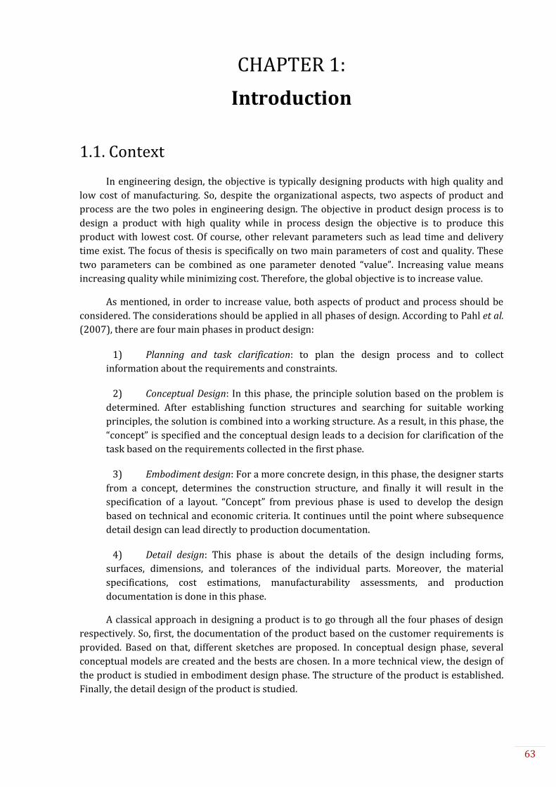
63
CHAPTER 1:
Introduction
1.1. Context
In engineering design, the objective is typically designing products with high quality and
low cost of manufacturing. So, despite the organizational aspects, two aspects of product and
process are the two poles in engineering design. The objective in product design process is to
design a product with high quality while in process design the objective is to produce this
product with lowest cost. Of course, other relevant parameters such as lead time and delivery
time exist. The focus of thesis is specifically on two main parameters of cost and quality. These
two parameters can be combined as one parameter denoted “value”. Increasing value means
increasing quality while minimizing cost. Therefore, the global objective is to increase value.
As mentioned, in order to increase value, both aspects of product and process should be
considered. The considerations should be applied in all phases of design. According to Pahl et al.
(2007), there are four main phases in product design:
1) Planning and task clarification: to plan the design process and to collect
information about the requirements and constraints.
2) Conceptual Design: In this phase, the principle solution based on the problem is
determined. After establishing function structures and searching for suitable working
principles, the solution is combined into a working structure. As a result, in this phase, the
“concept” is specified and the conceptual design leads to a decision for clarification of the
task based on the requirements collected in the first phase.
3) Embodiment design: For a more concrete design, in this phase, the designer starts
from a concept, determines the construction structure, and finally it will result in the
specification of a layout. “Concept” from previous phase is used to develop the design
based on technical and economic criteria. It continues until the point where subsequence
detail design can lead directly to production documentation.
4) Detail design: This phase is about the details of the design including forms,
surfaces, dimensions, and tolerances of the individual parts. Moreover, the material
specifications, cost estimations, manufacturability assessments, and production
documentation is done in this phase.
A classical approach in designing a product is to go through all the four phases of design
respectively. So, first, the documentation of the product based on the customer requirements is
provided. Based on that, different sketches are proposed. In conceptual design phase, several
conceptual models are created and the bests are chosen. In a more technical view, the design of
the product is studied in embodiment design phase. The structure of the product is established.
Finally, the detail design of the product is studied.

64
In this approach, sometimes designers achieve a perfect designed product with high
quality, but the cost of producing the product is not reasonable. This can be due to the
requirement of a complicated manufacturing machine to produce the product or sometime, it
may not be even possible to produce such product with existed machines and tools (Lack of
manufacturability). So, designers should go through all the stages of their design to create a
more manufacturable, cost-effective product. Often, designers need to repeat this process many
times and change the design entirely. Thus, the design process becomes more expensive and
time consuming.
Due to these issues, the concept of Integrated Product/Process Design (IPPD) is presented
in literature and is used in many industries such as automotive or aerospace. This concept
proposes concurrent designing of a system in both aspects of product and process. Concurrent
designing or IPPD is the domain of this study.
IPPD consists of product design, process design and production processes. While in the
process of designing a product, it is necessary to bear in mind the ease of production, agility,
maintenance, and flexibility, in the process of designing a manufacturing process, one needs to
think about the quality in product, product tolerances, satisfying customer’s needs, cost of
control and etc. From these points of view, the concurrent design is the best solution.
Figure 1.1 illustrates the necessity of the concurrent designing as explained. The objective
in product design domain is increasing quality while in process design domain is decreasing
cost. In process design product requirements should be taken into account in the choices such as
tools, machines, process etc. In product design process, manufacturability of the product should
be considered.
Product design(Quality)
Process design(Cost)
Product requirements
Process requirements
Figure 1.1. The necessity of concurrent designing due to two aspects' interactions
Each of these domains has its own difficulties. One of the main sources of difficulties is
coupling of the elements of design. For instance, in product design, there are coupling between
two or more features because of their interaction and/or assembly. In process design, the tools
should be adaptable with the machines. The process is defined based on the availability of
operators and machines etc.
Besides, there are inter-domain elements’ couplings too. There are so many relationships
between the elements of product design such as features, materials, connections, smoothness,
assemblability with the elements of process design such as cost of tools and machines, machine
precision, lead time etc. in addition to considerations such as process sequence, inspection
planning, storage limitation etc. These relations are not clear for the designer while designing a
new product. Although, the related features, e.g. machine capability, might be known, identifying
all the critical relations is not easy. So designer needs to find the answers of the following
questions:
How the product specifications limit the process?
How manufacturability of a product limits its design?
How the cost of manufacturing the product effects on the product design?

65
How the specifications of a product are related to its functioning?
How the specifications of manufacturing process are related to the cost and
productivity of the process?
What are the important specifications to design an unknown product?
All these issues create “complexity” in understanding the system. In addition to identifying
the links among elements, various uncertainties in concurrent designing increase the level of
complexity. Complexity notion is discussed in the following paragraphs.
There are so many articles and different point of views about the concept of complexity in
design. With increasing customer expectations, technology advancement and transdiciplinarity,
complexity in designing a robust product has become one of the main challenges for designers.
In order to design products with high standards, designers need to manage various issues which
lead to complexity.
Complexity can be referred to many concepts in different domains and sometimes it is
confused with complicatedness. A complicated system or product is not simple but knowable
such as a car or an aircraft (Elmaraghy et al., 2012). Complexity is where there is uncertainty.
For instance, development of a car requires engineering business knowledge in various
disciplines and as the design is not fully knowable, it is “complex”.
The issue of complexity can be seen from different points of views. Weber (2005) focuses
on qualitative and quantitative product and product development complexity, its measurement
and formalisation. Weber introduces five dimensions for complexity: Numerical,
Relational/Structural, Variational, Disciplinary, and Organizational complexity. ElMaraghy
considers three types of product, process and operational complexities for manufacturing
systems (Elmaraghy et al., 2012; W. ElMaraghy & Urbanic, 2003). In a more developed
classification presented in (Elmaraghy et al., 2012), product and process complexity is discussed
in addition to market and social factors. Suh (Suh, 2005a, 2005b) defines complexity as a
measure of uncertainty. The uncertainty can be in understanding the behaviour of the system, in
identifying and achieving the Functional Requirements (FR), or time-related.
So, the main source of complexity is uncertainty. Uncertainty can be in different forms. In a
classical taxonomy, it is divided into aleatory and epistemic. Aleatory uncertainty is the inherent
randomness of a phenomenon. Epistemic uncertainty is due to the lack of knowledge of the
system (Dantan, Qureshi, Antoine, Eisenbart, & Blessing, 2013; Kiureghian & Ditlevsen, 2009).
Thunnissen (2005) added two more categories to this classification: ambiguity and interaction,
for study of complex multidisciplinary systems. Ambiguity uncertainty is regarding the
miscommunication of different disciplines. Interaction uncertainty is ascending from
unanticipated interaction of events/elements in different levels/phases of design. Explicitly in
modelling and simulation, (Walter, Storch, & Wartzack, 2014) categorized uncertainty into
“uncertainty in data”, “uncertainty in model and simulation”, “phenomenological uncertainty”
and “uncertainty in human behaviour”.
Therefore, in order to manage complexity in IPPD, uncertainty should be managed and the
domains’ links in addition to inter-domains’ links should be identified. Achieving this aim is
possible by systematically modelling the product and its manufacturing process before
designing the product and process. This modelling process should be done in both domains
concurrently. In modelling process, to design and analyse a system, it is important to manage
these types of uncertainties in different phases of design. This management leads to reduce
unnecessary complexities in design process.

66
In order to manage complexity in concurrent designing, first, the objective should be
specified. As aforementioned, the objective in IPPD is increasing value which includes increasing
product quality and reducing process cost. Product quality can be also defined as customer
satisfaction. In process design, by decreasing cost, productivity should not be reduced. In IPPD,
all these objectives should be satisfied concurrently. So, a balance should be created. This
balance is by creating a proper link between product and process model and modelling two
domains concurrently.
The methodology used to model the system should be capable of modelling product and
process. So, it must have a framework to be applicable in both product and process. Moreover, it
should have a systematic approach to minimize uncertainty. In addition to having a common
framework, a similar approach of modelling product and process can assure the coherence
between two aspects.
Keeping this in mind, there are several design theories, methodologies and modelling
approaches from literature that are presented in Chapter II. The goal is to find an approach to be
applicable in IPPD conducting to robust design. A Robust design is defined by Suh as “a design
that is able to accommodate large variation in design parameters and process variables and yet
still satisfy the functional requirements” (Suh, 2005a). In other words, the design should be
insensitive to parameters’ variation. A robust design should be achieved by a robust model. The
concept of robust model is directly related to the managing uncertainties in the system. So, in
order to manage uncertainty a robust model is needed to be applicable in both product and
process design process.
Regarding this context, the following research questions are being asked.
1.2. Research questions
Thus, due to today’s industry needs, the concept of concurrent designing should be
explored to recognize how this concept can profit industry. The objective in this concept is to
increase “value”. So the first question is: How concurrent designing can benefit the industry and
how one can assess value in this concept?
As mentioned, the main challenge in concurrent designing is “complexity” caused by
various reasons. Therefore, the sources of complexity should be identified and a literature
review should be done to identify the solution(s) to manage complexity. Thus, the second
question is: How complexity can be managed in concurrent designing?
Uncertainty is the main source of complexity. The topic of uncertainty management is
discussed in literature as both individually and part of complexity topic. In any way, design
uncertainty needs to be managed. So, the third question is: How to manage design uncertainty?

67
In order to manage complexity and uncertainty in design process, we choose modelling of
product and process as a strategy. So, “How a modelling approach or a group of methodologies
and tools can help the designer to manage complexity and uncertainty in concurrent designing?”
is the main question here. The modelling approach should be able to create a link between
product and process departments to have coherence in both aspects. The approach should be
able to model the product based on the customer needs. In addition, it should be able to model
the process based on product requirements. Thus, it should create a two-way relationship
between product and process design departments. Hence, “how to achieve such a model?” is the
fourth question in this thesis.
After clarification of the approach to model the product and process (that would lead to
manage complexity), it should aid the designer to analyse the system and eventually designing a
high quality product with low cost, or optimize an existing product and process to aim at higher
value. Therefore, the fifth question is “How the created model by the proposed approach can
benefit the designer to analyse and optimize a system?”.
As a summary, the following questions are the key research questions to answer in this
context:
1. How concurrent designing can profit industry and how to assess value in this
concept?
2. What are the sources of complexity in IPPD and how to manage them?
3. How to manage design uncertainty?
4. How to model an integrated product/process system systematically to increase
“value”?
4.1. How to achieve a robust approach to model a manufacturable product to satisfy
the customer needs?
4.2. How to achieve a robust approach to model the process based on the product
requirements?
4.3. How to create a link between product and process in concurrent designing?
4.4. How to create a common approach for both product and process to have
coherence in both aspects?
5. How the model can be used to analyse and optimize the system?
1.3. Research objectives
In order to answer the questions in section 1.2, which are the research’s and industry’s
gaps, the research objective of this thesis is specified as:
“To achieve a robust modelling approach in integrated product and process
design in order to optimise value of the product based on the customer needs.”
This approach is a robust model that manages uncertainty in different stages of the design.
The approach should consider both aspects of product and process including all their complex
links. This requires managing complexity in IPPD. The ultimate objective is to optimize the value
of the product which means increasing the quality while minimizing cost according to the

68
customer needs. Customer needs can be translated into functional requirements in modelling
point of view. So, the structural model should be based on the functional requirement.
Therefore, the approach should create a link between functional and structural descriptions.
Assuring the quality of the product means assuring its behaviour while functioning. On the other
side, manufacturability should be assured as well. So, the approach includes four domains;
functional domain, behavioural domain, structural domain and process domain.
1.4. Methodology
To achieve the research objective and answer the research questions, the following methodology
is used:
1) Study of the concept of concurrent design and its advantages.
2) Identification of the sources of complexity since the main challenge in IPPD is complexity.
3) Review of different methodologies in literature to find an approach to model the product
and process that can lead to complexity management.
4) Choose of the best models, theories or/and methodologies to be combined to create an
approach based on the criteria for IPPD.
5) Creation of the approach for product design based on customer needs.
6) If other tools or methods are needed, repetition of step 3 and 4 and completing the model in
step 5.
7) Experimentation of the product design approach on a case study.
8) A full experimentation of the product design approach on another case study to avoid
creating a case-based approach and assure the generality of the approach.
9) Improvement of the approach based on the result of the case study to assure the
applicability of the approach.
10) Extension of the product approach for process design to a common approach for both
product and process aspects of IPPD.
11) Experimentation of the product/process design approach on the same case study in step 8.
12) Modification on the product approach if needed, to assure the coherence between product
and process models.
13) Utilization of the result model created by the approach for system analysis.
14) Uncertainty analysis and management using the proposed approach
15) Utilization of the result model created by the approach for optimization.
16) Summarizing the work and contributions
Based on this methodology, the thesis is structured.

69
1.5. Thesis outline
Chapter 1: The first chapter, which is presented here, started with an introduction of the
concept to emphasize the problem. Research questions are indicated and the
research objectives are specified accordingly. The methodology used to achieve this
objective is shortly presented.
Chapter 2: In chapter 2, state of the art for different concepts is presented. The chapter starts
with global needs of today’s industry. The objective is to increase value in both
aspects of product and process. In the second section, the notion of value is defined.
As a known solution for value improvement, the concept of concurrent designing is
presented. The main problem in concurrent designing is identified as complexity.
So, state of the art for complexity is presented in the fourth section.
In order to deal with complexity toward increasing the value, a methodology is
required to satisfy certain criteria. These criteria are specified in chapter 2. Various
theories, methodologies and approaches are studied and compared according to the
criteria.
After this literature review and regarding the criteria, Characteristics-Properties
Modelling (CPM) (Weber, 2005a) is chosen to identify the important parameters of
the system and to be used as a modelling framework of product. Due to the lack of
systematic approach of CPM, the hierarchical decomposition approach of Axiomatic
design (Suh, 2001) is used for decomposition of the system in a multi-level
environment.
Chapter 3: Chapter 3 is the proposition of this thesis for modelling a mechanical product and
to give a track to the designer for decision making in design process. In order to use
CPM for modelling a product and reduce complexity, an extended version of CPM is
proposed to be more applicable for complex system and being integrated in a
systematic approach. In this version, the system’s element distinction method of
CPM is used and also the model of product is similar. However, CPM uses an
approach called Property-Driven development to gradually create the model of
product by several analysis-synthesis cycles. Instead, in a systematic top-down
approach and using the decomposition approach of Axiomatic Design, the
extended-CPM creates the model of a product. Similar to Axiomatic Design, the
proposed systematic approach includes two domains of functional and structural.
The main challenge in reducing design complexity by modelling the system is to
identify the link between function and structure. So, Energy Flow Modelling (EFM)
is used to create this link. EFM models the behaviour of a system and helps to
identify the relations in CPM. So, the approach which uses EFM, CPM and axiomatic
design, is presented in this chapter.
In the last section of this chapter (section 3.4), a case study is used for
demonstration of the application of the approach (Malmiry, Pailhès, et al., 2016).
The studied case is a typical hair dryer. It is chosen because of familiarity of design
society with functioning of it and also because there are so many studies that used
it for presentation of their methods. So, this case study can be used to compare the
proposed approach of this thesis with other methods and approaches.

70
Chapter 4: The approach in chapter 3 is applied on hair dryer only for a better understanding
of the approach. So, several aspects are simplified. For a more detailed
implementation of the approach, an oil pump is used as a case study. So, in chapter
4, after a general literature review on oil pumps, a primary analysis is done on an
oil pump mostly for customer need’s analysis. Then, using the proposed product
modelling approach, the oil pump is modelled in detail. This implementation is
done based on the customer requirement as if the product does not exist. Though, it
can be used for optimization of the product as well. The case study is an external
gear oil pump used in Renault®.
Chapter 5: Chapter 5 is the exploitation of the proposed approach to show how the proposed
approach can be used for uncertainty management and complexity management.
Despite the advantages of the approach, the created model using CPM and flow
modelling can be used in three different ways. So, this chapter focuses on the
application of the product approach modelling and its result and not IPPM
approach. So, this chapter is divided into 3 sections:
Since uncertainty is the main source of complexity, section 1 is the application of
the approach for uncertainty management. It is to illustrate how the approach can
reduce complexities caused by uncertainties. The section starts with a short
literature review about different types of uncertainties and then, using the
approach, it is shown how each of these types can be managed.
Section 2 is sensitivity analysis of the case study. Thanks to the created
mathematical relations, the model can be used to analyse the effect of product
characteristics on the output of the system. So, a local and global sensitivity analysis
is used on the product model and the result is presented in this section. By these
analyses, the key parameters that are effective on the performance are identified.
The third section illustrates how the approach and its result can be used in
tolerancing. After identifying the relations by the proposed approach, tolerance
analysis can be done. So, in this section, tolerance analysis which is also a kind of
sensitivity analysis is discussed in general and it is demonstrated on the case study
of chapter 4. Therefore, the key tolerances are determined by this study.
Chapter 6: Chapter 6 is our proposition for modelling a mechanical system in concurrent
design environment. To assure the coherence between product design and process
design, the same concept for product modelling is proposed for modelling of its
process. Instead of EFM, material flow and information flow (MF/IF) are used to
model the process. Using the framework of CPM in both product and process
assures the coherence between two aspects. In addition, the proposed model for
IPPD is the extension of product model.
The second section of chapter 6 is the case study to present the proposed
integrated product/process modelling approach in action. The same case study
(external gear oil pump) is used to emphasise the extension and identifying the
relations.
In the third section of this chapter, it is shown how the proposed Integrated
Product/Process Modelling (IPPM) can be used for optimisation. Using the
sensitivity analysis and tolerance analysis of chapter 5, and adding cost

71
considerations, the result of the model can be used for optimising a system.
All the chapters are summarized and along with contributions, limitations and future
work, it is presented in conclusion. The thesis map in an illustration is presented in Figure 1.2.
1) LR: Concurrent design
2) LR: Complexity
3) LR: DTMs
4) Choosing the best
5) Creation of the Product design approach
6) Repetition of step 3 and 4.
7) Experimentation: Product design approach
8) Experimentation: Product design approach on another case study
9) Improvement of the product design approach
10) Concurrent design approach
11) Experimentation: Concurrent design approach
12) Modification on the product approach for concurrent design.
13) Sensitivity analysis
14) Uncertainty management
15) Tolerance optimisation
16) Conclusion
6. IPPM
5. Uncertainty & Complexity management
4. Case study
3. Product
2. Literature Review
1. Introduction
1.1. Context
1.2. Research questions
1.3. Research objectives
1.4. Methodology
1.5. Thesis outline
2.1. Context
2.2. Value
2.3. Concurrent designing
2.4. Complexity
2.5. DTM
3.1. Context
3.2. Extended-CPM
3.3. Energy flow modelling
3.4. Product modelling approach
3.5. Mini case study
4.1. Oil pump
4.2. Product model
4.3. Complementary tools
5.1. Uncertainty management
5.2. Sensitivity analysis
5.3. Tolerance analysis
6.1. Context
6.2. Flows
6.3. CPM in IPPD
6.4. IPPM approach
6.5. Case study
6.6. Tolerance optimisation
Research questions
1. How concurrent designing can profit industry and how to assess value in this concept?
2. What are the sources of complexity in IPPD and how to manage them?
3. How to manage design uncertainty?
4. How to model an integrated product/process system systematically to increase �value ?
5. How the model can be used to analyse and optimise the system?
M e t h o d o l o g y
Conclusion
Figure 1.2. Thesis map

72
CHAPTER 2
1) LR: Concurrent design
2) LR: Complexity
3) LR: DTMs
4) Choosing the best
5) Creation of the Product design approach
6) Repetition of step 3 and 4.
7) Experimentation: Product design approach
8) Experimentation: Product design approach on another case study
9) Improvement of the product design approach
10) Concurrent design approach
11) Experimentation: Concurrent design approach
12) Modification on the product approach for concurrent design.
13) Sensitivity analysis
14) Uncertainty management
15) Tolerance optimisation
16) Conclusion
6. IPPM
5. Uncertainty & Complexity management
4. Case study
3. Product
2. Literature Review
1. Introduction
1.1. Context
1.2. Research questions
1.3. Research objectives
1.4. Methodology
1.5. Thesis outline
2.1. Context
2.2. Value
2.3. Concurrent designing
2.4. Complexity
2.5. DTM
3.1. Context
3.2. Extended-CPM
3.3. Energy flow modelling
3.4. Product modelling approach
3.5. Mini case study
4.1. Oil pump
4.2. Product model
4.3. Complementary tools
5.1. Uncertainty management
5.2. Sensitivity analysis
5.3. Tolerance analysis
6.1. Context
6.2. Flows
6.3. CPM in IPPD
6.4. IPPM approach
6.5. Case study
6.6. Tolerance optimisation
Research questions
1. How concurrent designing can profit industry and how to assess value in this concept?
2. What are the sources of complexity in IPPD and how to manage them?
3. How to manage design uncertainty?
4. How to model an integrated product/process system systematically to increase �value ?
5. How the model can be used to analyse and optimise the system?
M e t h o d o l o g y
Conclusion

73
CHAPTER 2:
Literature Review
This chapter is a general literature review including the domain, the research problem in the domain, and studying the possible solution in literature. The first part explains the need of today’s industry. The objective in industry is to increase “value”. So, in the second section this notion is defined. Increasing value includes two aspects of product and process. Concurrent designing is chosen as the best solution for increasing value considering both aspects. This concept along with other related topics are discussed in the third section. After literature review of concurrent designing, “complexity” is identified as the main problem to deal with. So, in the fourth section, definitions, classifications and different solutions for design complexity are discussed. In order to deal with complexity while improving value, a systematic approach to model the system with specific criteria is required. In section 5, various theories, methodologies and approaches are studied to find a solution for complexity in design. In case of the absence of a suitable methodology for the problem, a combination of methods/approaches will be used, an existing method/approach will be extended or a new method/approach is developed.

74
2.1. Context
In the last decades, the evolution of manufacturing systems was from craft production to
mass production and after using lean manufacturing systems, today to mass customization with
the cost of mass production. There are several ways for implementation of mass customization;
Self-customization, where the customer can customize the product based on his/her needs,
customization using a mixed of standard procedures, modular product architecture, and flexible
customization (Magrab et al., 2010). Figure 2.1 demonstrates the transition of manufacturing
paradigms in the last 100 years (Koren et al., 2013; Koren, 2010).
Figure 2.1. Evolution of manufacturing paradigms (Koren et al., 2013)
“Mass individualization” (MI), also known as “Personalized Production” is a new trend
which means to satisfy all aspects of customer’s expectation by participating them in the design
process. Unlike mass customization which customers have several options to choose, in MI the
customer can not only choose between various suppliers, actually design instead of choosing
among options (Koren et al., 2013). In fact, the customer will participate in all the variety levels
such as design, fabrication, assembly, sales or use (Hu et al., 2011). Personalization in MI means
having very small fixed cost, short set-up time (additive manufacturing) and after-sale
customization. Also the adjustments of regional personalization based on the environment,
culture, etc. need to be deliberated. MI creates huge variety of products and features which it is
essential to manage it (H. ElMaraghy et al., 2013). On the path of mass individualization,
products with adoptability, changeability, self-diagnosis, self-resilience, self-improving
environment paradigm and co-creation, while satisfying the required function are the needs of
the market (Tolio et al., 2010).
In mass customization or mass individualization, modifications and decision making in
different level of design in a multi-scale system is required. Systematically, modelling a system in
this environment can reduce the cost of development and minimize the errors. Modelling in
product design can be referred to functional modelling or/and structural modelling. Functional

75
modelling assures that the system works based on the required function. Structural modelling is
the study of components design and their assembly.
While the objective in product modelling is normally increasing quality, the cost refers to
both product and process modelling. The major part of cost is related to process of producing
the product in early stages. The source of these cost are: material, manufacturing process,
assembly process, machines, tools, operators, fixed costs and etc. We refer to these activities as
“process”. So, the objective of process domain is minimizing cost. However, the product-side
objective (maximizing quality) should be satisfied while the functional requirements are met.
Therefore, both product and process modelling should be done concurrently (Finger et al., 1992;
Sapuan, Osman, & Nukman, 2006; Soundar & Bao, 1994).
During the evolution of manufacturing systems, and especially in mass customization and
MI, the global objective is to increase “value” (Daaboul et al., 2011; Elmaraghy et al., 2012; Koren
et al., 2013; Tseng & Jiao, 1998). However, value can be referred to different subjects. In the next
section, the definition of value in this thesis will be presented.
2.2. Value
The meaning of “value” is given by the context. So it has different meanings and definitions
depending on the field of study. In finance, value is the creation of wealth for stakeholders. In
human resource, it refers to the skills of the employees. In marketing, value is what the customer
is ready to pay for a product (L. A. Shah, 2012). However, in all these fields, value is what we care
about. In design and manufacturing, and specifically in this thesis, value refers to the value of a
product for the organization and the customer. So the basis of value is the triptych of customer-
product-company. Thus, the company materializes value into a product or a service in order to
satisfy a customer by spending its resources (Ahmed & Yannou, 2003). So there are two sides;
company and customer. The goal of company side is to increase the benefit, and the goal of
customer side is to increase the satisfaction. One of the approaches for increasing benefit is to
decrease cost of production. Therefore, value is simplified into two aspects of customer
satisfaction and cost of process. So “value” mathematically can be defined1 as Eq. 1.1.
𝑉𝑎𝑙𝑢𝑒 =𝐶𝑢𝑠𝑡𝑜𝑚𝑒𝑟 𝑆𝑎𝑡𝑖𝑠𝑓𝑎𝑐𝑡𝑖𝑜𝑛
𝐶𝑜𝑠𝑡 𝑜𝑓 𝑝𝑟𝑜𝑐𝑒𝑠𝑠 (1.2)
Conversely, this definition is very general. As mentioned, satisfaction for our customer
means faultless functioning of the product. By relating the function of the product, (Yannou,
1999) modifies the mathematical definition of value as followed;
𝑉𝑎𝑙𝑢𝑒 = ∑ 𝐼𝑖 × 𝑉𝑎𝑙𝑢𝑒𝑗(𝑓𝑢𝑛𝑐𝑡𝑖𝑜𝑛 𝑖) = ∑ 𝐼𝑖 ×𝐼𝑖 × 𝑆𝑖𝑗
𝐶𝑖𝑗𝑓𝑢𝑛𝑐𝑡𝑖𝑜𝑛 𝑖𝑓𝑢𝑛𝑐𝑡𝑖𝑜𝑛 𝑖
(1.3)
Where,
𝐼𝑖 Importance of a function i 𝑆𝑖𝑗 Satisfaction of function i in scenario j
𝐶𝑖𝑗 Cost of function i in scenario j
1 This definition is not a precise mathematical equation. It only aims to mathematically illustrate that
increasing value means increasing customer satisfaction and decreasing cost of process.
76
In designer’s point of view, customer satisfaction can be defined as the quality of the
product. This includes the amount of knowledge that the designer has about the designing
system (Xu & Bernard, 2011). Moreover, the cost of function can be defined as the “cost of
process”, meaning the cost of manufacturing or providing a product. So, the cost estimation and
related methods (Bosch-Mauchand, Siadat, Perry, & Bernard, 2012; Mauchand, Siadat, Bernard,
& Perry, 2008; Perry, Mauchand, & Bernard, 2006) need to be integrated in this concept too. In
this way, the value is defined by both sides of product and process.
In a process, a series of activities that adds value to an article and transfer the input into
output is called “value chain”. These processes or activities could be production, marketing or
after-sale service. According to the definition of (Kaplinsky & Morris, 2001), “The value chain
describes the full range of activities which are required to bring a product or service from
conception, through the different phases of production (involving a combination of physical
transformation and the input of various producer services), delivery to final consumers, and final
disposal after use.”
Basically any person, machine, process, product or brand that adds value to a product or
service considers as value chain (Mascarenhas, 2004). In order to increase value, we need to
consider all aspects of product and process through the whole life cycle. These aspects are
durability, adoptability, reliability, serviceability, recyclability and disposability. In order to
improve every value chain, there is a need to improve the quality, decrease the cost, to follow the
schedule and to meet the user requirements.
Initially, a simple value chain consists of four stages of design, production, marketing, and
consumption and recycling. Our focus is on the first stage of the chain yet considering the three
other stages.
In rapid globalization, toward mass customization and MI, value chain has an important
role. According to (Kaplinsky & Morris, 2001) there are three reasons for the importance of
value chain;
1. With the growing division of labour and the global dispersion of the production of
components, systemic competitiveness has become increasingly important.
2. Efficiency in production is only a necessary condition for successfully penetrating global
markets.
3. Entry into global markets which allows for sustained income growth – that is, making the
best of globalization - requires an understanding of dynamic factors within the whole
value chain.
The first research question (section 1.2) includes assessing value. Value needs to be
assessed in the whole process. This can be done by analysing the value chain and identifying the
value-added activities in the chain. This analysis and identification is known as “value chain
analysis”.
From 1985 when Michael Porter (Porter, 1985) introduced a method for value chain
analysis and emphasized the importance of it, many articles tried to cover different aspects of
value chain: General concept of value chain analysis (Kaplinsky & Morris, 2001; Mcguffog &
Wadsley, 1999; McPhee & Wheeler, 2006; Yang, Luo, Li, Yang, & Lee, 2013), case studies on
specific product and industry (McEachern & Schröder, 2004), or with focus on global aspect of
each product/industry (Wad, 2008; Walters & Lancaster, 2000). Also, there are many articles on
the management aspect (Balkau & Sonnemann, 2010; Mcguffog & Wadsley, 1999), modelling of
value chain (Roper, Du, & Love, 2008) or in the direction of Mass Individualization (MI) as the

77
involvement of customer in the value chain (Mascarenhas et al., 2004; McEachern & Schröder,
2004), and finally the evaluation of value chain (Swafford, Ghosh, & Murthy, 2006). Yet, most of
these studies are based on the basic model of Porter.
The value chain needs to contain changeable and reconfigurable process to achieve a
variety-oriented manufacturing system. Overall, we need a balanced system. A balanced system
is stable but flexible. It has the economy of scope and scale. It maximizes the productivity while
minimizing the wastes. To achieve a balanced concurrent system, we need to re-design the
products, processes and services by eliminating, reducing and replacing the necessary elements.
Risk management however must be part of the re-designing process. So, the process must be
robust to have a robust product as the result. A robust design of process as (H. ElMaraghy et al.,
2013) stated is capability to reuse or re-combine an existing manufacturing, organizational and
supply chain resources to fulfil a stream of differentiated customers’ needs.
In implementation of value chain, the majority focused on designing a new chain. Few
articles focused on optimization and improvement of the chain. All these articles analyse the
process of production to increase the value and not enough studies are done considering both
product and process aspects. A robust methodology for achieving this goal is still a challenge in
industry. Industry uses several approaches to address different issues in this domain. Either
they are outdated and not adoptable for today’s complex systems or not well-developed. So, a
well-developed robust approach that is understandable and easy to use for industry is required.
Thus, in order to assess and increase value in industry, different aspects of both product
and process should be taken into account and improved. A known paradigm is concurrent
designing which is designing a product and its process simultaneously. Concurrent designing
which is also known as Integrated Product and Process Design (IPPD) is one of the best solution
for mass customization (Tseng & Jiao, 1998) and mass-individualization. Next section explains
this paradigm and its related concepts.
2.3. Concurrent designing
In conventional engineering practice in the past, design and manufacturing had separated
departments. This separation and sometimes isolation of departments led them into costly and
time consuming process of product development. As Figure 2.2 illustrates the cost in different
phases of a product life cycle, it is apparent that the most costly phases are concept formulation
and validation. However, in traditional approaches, the involvement of the manufacturing
department was in phase 6 as pointed in Figure 2.2, meaning, after 75% of the cost of
development is spent. Some difficulties in manufacturability of the product would have led the
designers to redesign the product and repeat the previous phases. Because of this costly and
time-consuming process, the concept of concurrent design is introduced.
In literature, many terms have been used for concurrent designing to describe similar
approaches such as Integrated Product/Process Design (IPPD), Integrated Product and Process
Design and Development (IP2D2), simultaneous design, and design fusion. There are also related
concepts such as feature-based design, design for manufacturing (DfM), and design for assembly
(DfA). This section is an overview of these concepts to specify the domain of the thesis but it is
not a complete state of the art for concurrent designing.

78
Figure 2.2. Life cycle phases (R. Liu & Yang, 2001)
2.3.1. Integrated Product and Process Design (IPPD)
Integrated Product and Process Design (IPPD) means concurrent designing of product and
process. As Magrab et al. (2010) stated in the book of “Integrated Product and Process Design
and Development” (IP2D2), the overall goal of an IP2D2 team is to obtain the following results:
High customer satisfaction.
Minimum product cost with high profitability.
Equalled or surpassed competitively established benchmarks.
Short time-to-market.
Lower product development cost.
High quality.
High factory throughput with minimum work-in-progress.
Minimum space, handling, and inventory of raw materials and finished goods.
Increased utilization of automation and fuller utilization of existing equipment.
Elimination of redesigns and engineering changes.
Broadened product line, with considerable variety.
Early supplier involvement.
So, the overall aim is “producibility”. The terms of producibility refers to the fact that how
easy a product can be made which includes the factors of
Design, from embodiment design and sketching until the final design of product and
processes
Scheduling and meeting the customer needs in logistics, retail and after-sale

79
Quality including the eight dimensions as Garvin (1987) has proposed which are
performance, features, reliability, conformance, durability, serviceability, aesthetic and
perceived quality. (Garvin, 1987) and
Cost, including the cost of product, overhead and indirect cost, hidden cost, design and
manufacturing cost, and sustainment costs. (Life cycle, operation and support)
In an integrated product and process system, the components of product and process are
fully related to each other and therefore the design process must be done concurrently. Table
2.1, gathered all the elements of product and process in a value chain with of course many
overlapping elements. In addition to these overlaps, there are requirements in the product that
need to be satisfied in the process and vice versa. The overlaps and the two-way requirements
make concurrent designing crucial.
Table 2.1. The factors in product and process design (Magrab et al., 2010)
Product Design Process Design
Function, usability Performance characteristics Environment Features Technology/innovation required Analysis and simulation Prototypes Producibility Material selection Manufacturing methods Handling and presentation Fabrication/assembly Number of parts and part variation Documentation/engineering drawings Human factors/ergonomics Appearance and style (aesthetics) Configuration Modularity enhancements Degree of standardization Reliability Patents
Responsiveness Delivery date to customers Packaging and shipping Adaptability to variability in materials and process conditions Integration of new process technology into existing system with minimum disruption and cost Maximum responsiveness to surges in demand Minimum changeover time and cost Maximum production flexibility Quick turnaround capability Maximum product family Design-dependent Assembly methods Waste Manufacturing methods Materials Factory characteristics Material handling and flow Work station design (ergonomics) Manufacturing equipment capabilities and Reliability Floor layout Plant location Safety Training of factory personnel Waste management Production Quality control Capacity/production rate Production planning, scheduling, and purchasing Transition into production of existing products Outsourcing of parts and subassemblies Suppliers Documentation
Many literatures, with confirming the advantages of concurrent designing, integrated
different common tools to this concept. These tools include and not limited to Finite Element
Analysis (FEA) tools (Giudice, Ballisteri, & Risitano, 2009), Game theory (Badhrinath & Rao,
1996), Virtual prototyping and rapid prototyping (Chang, Silva, & Bryant, 1999) Quality
Function Deployment (QFD), Failure Mode and Effect Analysis (FMEA), and Analytic Hierarchy
Process (AHP) (Hsiao, 2002). The goal was to use these tools to solve different issues that the
designers are facing in implementing concurrent designing. Though, not all issues are solved yet.

80
Ha & Porteus (1995) focus on simultaneous review of two aspects in concurrent designing.
Simultaneous review has two advantages. First, available information for process design
department in each stage of design instead of the final stage enables the parallel development in
both departments. Second, quality control in each step saves time and resource required for
redesign. In addition, Soundar & Bao (1994) accentuate the importance of measuring
manufacturing system performance in design using concurrent designing methodologies.
Furthermore, (Nguyen & Martin, 2015) focuses on process selection and planning in IPPD.
One aspect of IPPD is material design and its integration in product and process design. It
includes material selection which is a decision making process to satisfy required performance
specifications (Ashby, Bréchet, Cebon, & Salvo, 2004), concurrent designing of materials and
structure in a multi-scale modelling (McDowell & Olson, 2009) and material integration
(McDowell et al., 2010). Another aspect in IPPD is market considerations. Andreasen (1987;
1994; 1996) and (Godot, 2013) propose an integrated product development strategy including
three aspects of product, process and market. These two aspects of IPPD (Material design and
market) are not the focus of this thesis.
Various case studies can be found in literature on application of IPPD in systems that are
considered as complicated or where there is complexity in design. Wang & Wright (1996)
propose IPPD for designing electromechanical parts while two departments of mechanical and
electrical design should coordinate and cooperate, the electrical and mechanical CAD tools
should be used concurrently. Other examples of case studies include designing a short haul civil
tiltrotor (Marvis et al., 1997), manufacturing transmit/receive modules in microwave systems
(Karne et al., 1997), designing and optimization of an airplane engine (Chang et al., 1999),
designing a Pico radio test bed (Odell & Wright, 2002), designing wearable computers (Finger,
Konda, & Subrahmanian, 2009), and designing and implementation of a Fresnel thermodynamic
solar plant (Malmiry and Perry, 2013). In this thesis, the modelling of an oil pump in both
aspects of product and process is studied (chapter 4 and chapter 6). An automobile oil pump is
relatively a simpler case but considering the coupling of elements, uncertainty, and state
variability of the system, it is complex to design. These make it a good example for
demonstration of an approach to manage complexity.
2.3.2. Feature-based design (FBD)
Feature-based design (FBD) is another concept in the domain of concurrent design to
create a link between product features and the process of manufacturing including process
planning, machining and inspection (Salomons et al., 1993). FBD is a design system where the
product design is decomposed into features. Feature is “a semantically endowed object that
accompanies product development from the customer request through to product release” (J. J.
Shah, 1991). The process is defined based on the required operations for creating the required
features of product. Therefore, the link between product and process departments is created.
Three main views in FBD are feature recognition, design by features, and interactive
feature definition. So, FBD can be divided into product design point of view (Pratt, 1984) and
process planning point of view (Alting & Hongchao, 1989; Ham & Lu, 1988; J. Shah, Sreevalsan, &
Mathew, 1991). Pham & Ji (1999) focus on application of feature-based design in machining.
They emphasize the importance of the information flow about manufacturability assessment,
machining schemes, cutting parameters, and surface finish and CAD model in both departments.
Cherng et al. (1998) propose feature-based modelling for Rapid Response Manufacturing where
the objective is satisfying customer requirement in minimum time. Moreover, Changchien & Lin

81
(2000) propose another methodology in IPPD to be used in feature-based design and
optimization design.
The concept of designing process based on product features is interesting in process
design decision making. Decisions such as machine, tools and operators’ skills are made based
on product entities. The weakness of FBD is its structural point of view. In modelling a system in
concurrent designing, the product function should be considered too. Moreover, FBD is very
effective for optimizing and existing product while it becomes inefficient in designing new
products. Moreover, a dynamic concurrent designing is preferred than a static concurrent
designing like FBD to consider the performance of the product while it is functioning.
To sum up, collaborative modelling in order to increase the level of knowledge in both
departments of product and process is crucial. So, as Roucoules & Tichkiewitch (2015) also
mentioned, the solution is to create the link between function and feature (structure) by least
commitment.
2.3.3. Design for X (DfX)
As mentioned earlier, in IPPD, manufacturability is one of the main considerations. The
approach to design a product by considering its manufacturability is called Design for
Manufacturing (DfM). A similar approach is Design for Assembly (DfA) that involves assembly
requirements in the process of design. Design for X (DfX) is a generic name for a family of design
methodologies with a particular purpose. X can represent a specific property such as cost,
quality, lead time, efficiency, etc. or a life cycle phase of the product such as manufacturing,
assembly etc. (Huang, 1996; Tichem, 1997).
The objective of DfM is to include producibility early in design stage to minimize lead time
and cost of development while satisfying the customer (R. Liu & Yang, 2001). The satisfaction of
customer means respecting the performance, quality, delivery time, reliability, serviceability and
aesthetics.
Many studies have been done on DfM. Several of them present the concept of DfM, its
advantages and applications (G Boothroyd, 1994; Kuo, Huang, & Zhang, 2001; Nowak et al.,
2004; O’Driscoll, 2002). Swift & Booker (2003) focus on implementation strategies for DfM. They
analysed manufacturability and solution in different types of processes to improve design. In
addition, there are several articles and books about process selection and material selection
such as (Ashby et al., 2004; Edwards, 2003; Lovatt & Shercliff, 1998; Swift & Booker, 2003)
based on process classification and attributes selection. Besides, Esawi & Ashby (2003)
developed a technique to reduce cost in pre-selection of processes based on resource
consumptions.
Design for Assembly (DfA) is also an interesting concept in DfX for concurrent designing.
In most products, assembling parts is inevitable due to relative movement of components,
material differentiation, ease of producing subparts, possibility of replacement and upgrades,
differentiation of functions, the requirement of accessibility, and cost considerations (G
Boothroyd & Alting, 1992). In DfA, the objective is to reduce the number of components that
need to be assembled, ensure the ease of assembly of other components and to reduce the total
cost while satisfying the functional requirements. Some of the publications that discuss about
this concept are (Andreasen, Kähler, & Lund, 1988; G Boothroyd & Alting, 1992; Geoffrey
Boothroyd & Dewhurst, 1984; Redford, 1994).
82
DfA approach is focused on the assembly design. DfM approach has a more general
perspective in concurrent designing. However, both these approaches focus on the product
design based on process requirements or limitations. A two-way link is needed to
simultaneously design both product and process in different levels of decomposition.
2.3.4. Concurrent engineering (CE)
Concurrent engineering (CE) is another related concept which should not be confused with
concurrent designing. Concurrent designing is a part of concurrent engineering. CE has an
operational approach and includes enterprise considerations. It is an approach that focuses on
reducing lead time and improving the quality by integrating the product life cycle processes such
as product planning, design; production; delivery, service and end-of-life (Prasad, 1996). It gives
a framework for the whole process of design in different aspects. Concurrent engineering can be
considered as global view which concurrent design is part of it (Parsaei & Sullivan, 1993).
The goal of concurrent engineering is to be responsive to the market. Responsiveness has
two aspects: to meet the market demand by shortening the manufacturing cycle, and to meet
market opportunity shortening the product development cycle. Responsiveness is the winning
characteristics of any successful business with these two aspects (B. Wang, 1997).
There are several tools and methods for CE which can be used in concurrent design as
well. Figure 2.3 illustrates some of these methods in a manufacturing business including four
integral stages of implementation: product planning, product design, process engineering and
product and service. In (B. Wang, 1997) these tools in integrated product, process and
enterprise design are discussed.
All aforementioned concepts are trying to create a link between product design and
process of manufacturing the product. Thanks to this link and concurrent designing of product
and process, the department of process design enters in early stage of the product design.
Therefore design cost which is about 70% of product development cost is reduced and the
process of product development becomes faster.
However creating these links generates issues too. Issues in concurrent designing can be
categorised into five concepts (Shankar & Jansson, 1993):
1) Compatibility; including compatibility of material-process, configuration-process,
material-configuration, and availability of resources.
2) Complexity; because of intricacy (the amount of detail in parts), tolerance and surface
finish, symmetry, uniformity, accessibility, orientation, and ease of handling.
3) Quality; to have a robust design without features that cause critical flaws.
4) Efficiency; the design should consider efficiency in material usage, number of parts and
number of operations. Moreover, the variety should be low and the design uses mostly
standard parts.
5) Coupling; including material-based coupling, process-based coupling and configuration-
based coupling.
Regarding this categorization, the focus of this thesis is dealing with complexity as the
most important issue in concurrent designing. We consider compatibility as part of coupling
issue. Coupling is one of the main sources of complexity and the other important issue is

83
uncertainty. There are different definitions, classifications and proposed solutions for
complexity in product and process design that will be discussed in the next section.
Figure 2.3. Systematic concurrent engineering (B. Wang, 1997)
The aspect of quality, achieving a robust product, is taken as the objective of concurrent
designing which is to increase value. Thus, the first research question (section 1.2) can be
answered by the explanations of sections 2.2 and 2.3. It has been explained how concurrent
designing can benefit industry and how value can be assessed in this domain.
2.4. Complexity
This section is assigned to the concept of complexity which is the main difficulty in IPPD.
Complexity is one of the biggest challenges of the engineers and scientists and yet there is no
clear solution for it. The concept of complexity is discussed in various fields such as computer
science, biology, organizational science etc. Based on that, there are definitions and
classifications of the types of complexity. The focus of this study is complexity in concurrent
design. Therefore, the definition, classification and solution of complexity in this domain based
on different point of views are discussed and then the position of our study according to them
will be pointed out.
2.4.1. Definition of Complexity
As Elmaraghy et al. (2012) stated, there is no universal and precise definition of
complexity that can cover the meaning of this word in all fields. However, there are several

84
definitions for complexity based on the objective. For instance in optimization, complexity can
be defined as the number of effort required to formulate the optimization problem and identify
the optimal solution(s). Complexity can be caused by the competitive market because of the
market uncertainty and volatility, increase the variety, globalization, complex economic, socio-
political and technological dynamics, increasing in customer expectation with their possibility in
product comparison and also need to increase the company competitiveness (Elmaraghy et al.,
2012; Tolio et al., 2010).
Weber (2005b) discusses complexity in product development aspect. He also believes that
there is no general concept and might not be even possible to develop one. As he stated,
“complexity is too complex for conceptual representation”. In general, any discussion about
complexity leads to the fact that how we can measure complexity. So complexity is linked to
“information content”. Other than that he mentions randomness (or uncertainty) as the second
factor.
Suh, the creator of “Axiomatic Design”, in his book of “complexity”, defines complexity as
“a measure of uncertainty in understanding what it is we want to know or in achieving a
fundamental requirement (FR)” (Suh, 2005a). This definition of complexity, which is based on
Axiomatic design, implies “uncertainty” as the main cause of complexity.
2.4.2. Classification of Complexity
There are different classifications of complexity in literature. According to (Suh, 2005a),
complexity is divided into four categories;
1) Time-independent real complexity: As Figure 2.4 illustrates, the real complexity happens
when the design range doesn’t cover the system range which means the probability of
the FR is less than 1.0. For instance, the function of an oil pump is different when the
engine of the car is off or on, though, the designer doesn’t consider all the states of the
product in the design.
System range
Design range
Bias
Target
Probability
density
FR
Area within
common range
Figure 2.4. Design range and system range in axiomatic design
2) Time-independent imaginary complexity: The second category is the complexity caused
by the lack of knowledge of the system. The lack of knowledge means knowing the
function of the product in all possible states of the system. It also means knowing all the
related components of the system, including external components, and their exact
relationship and effects on each other. For instance, while we have to try to have a design
with good quality, yet there are defaults during the product functioning with unknown
reason(s).
3) Time-dependent combinatorial complexity: The third and fourth types of complexity,
unlike the first two, are related to the time and happen because of the uncertainty in
predicting the future. The combinatorial complexity occurs due to a continued expansion

85
in the number of possible combinations with time which may eventually lead to a chaotic
state or system failure. The effect of depreciation on the product functionality is a
common example.
4) Time-dependent periodic complexity: The periodic complexity only occurs in a finite time
period, resulting in a finite and limited number of probable combinations.
According to (Kim, 2004) there are four causes for complexity. This classification which is
also based on the axiomatic design is shown here with the resemblance in the axiomatic design:
1) when the design is coupled: Independence axiom violation
2) when the design is uncertain: Information axiom violation
3) when the design is decoupled and not solved in the particular sequence: Lack of
knowledge, and
4) when the design has many states: Non-equilibrium
Figure 2.5 illustrates this classification in a radar chart based on the axiomatic design.
Figure 2.5. Complexity classification of (Kim, 2004) based on axiomatic design
Weber (2005b) on the other side, more specifically about the product design, divides the
complexity into two categories of “connectivity” and “variety” (Figure 2.6). In case of the
connectivity, complexity occurs because of the type of connections and the number of
connections and in case of the variety it occurs due to the type of elements and number of
elements (Weber, 2005c).
Figure 2.6. Product development complexity categorization based on (Weber, 2005c)
In a more extended concept, Weber (2005b) divides complexity into five different
dimensions; Numerical complexity, Relational/structural complexity, Variational complexity,
Disciplinary complexity, and Organizational complexity. The first three dimensions refer to the
product design and the last two refer to the process of manufacturing (Figure 2.7). The focus is
on the product development, and the process is in fact the external effects on the product
development process.
Complexity
Connectivity
(diversity of relations)
Variety
(diversity of elements)
Types of relations Number of relations Types of elements Number of elements

86
Figure 2.7. Five dimensions of complexity according to (Weber, 2005c)
ElMaraghy (2012) gathered the points of view about complexity in (Elmaraghy et al.,
2012). While he has rather production point of view on complexity of design, he divided it into
three aspects of product, manufacturing process and business organizations. This point of view
is also an interest of this section because he tried to consider both aspects of product and
process as well as their relationship as sources of complexity (Figure 2.8).
Pro
du
ct a
nd
Hard
En
ab
lers
Customer
Requirement
Product
Complexity
Control Systems
& Software
Product Structure
Manufacturing
Technology
Design Tools &
Methodologies
Mfg. Systems
Responsiveness
Planning &
Scheduling
Human Cognitive
Ergonomics
Global Supply
Chain
Source of
Complexity
Pro
cess and S
oft E
nab
lers
Social and Environmental Pressures:
Government Legislation,
Standards
Complexity of
Market Forces: Global Competition,
Turbulence, Variety, Short Delivery, Zero Defects, etc.
Figure 2.8. Drivers of manufacturing complexity according to (Elmaraghy et al., 2012)
ElMaraghy et al. (2012) classify the types of complexity into static and dynamic. Static
complexities are structural, computational and algorithmic, size/volume/quantity, software
complexity and network interaction. Dynamic complexities are market turbulence, product
variety, scheduling, supply chain dynamics, operational/cognitive, and chaos and emergence.
2.4.3. Proposed Solutions for Complexity
Suh (2005) believes that the best way to deal with complexity is to reduce or eliminate it.
He justifies his method based on the classification of complexity. As it has already been stated, in
this method, the first type of complexity is real complexity which is due to not covering the
system range by the design range. To reduce real complexity, with respect to the independence
axiom, one must put the system range inside the design range and reduce the variance of the
system range. To reduce imaginary complexity which is due to the lack of designer’s knowledge
of the system, the exact relationship of the FRs and Design Parameters (DPs) of the system are
needed to be known. Suh believes by writing down the design equations, the need for trial-and-
error will be eliminated and the complexity will be reduced. The solution for combinatorial
complexity is to transfer it into periodic complexity. The idea is to disrupt the system in specific
time points and reinitialize the FRs.
Product
Numerical complexity
Relational complexity
Variational complexity
Process
Disciplinary complexity
Organisational complexity

87
On the contrary with Suh’s “complexity reduction” approach, ElMaraghy et al. believe that
complexity not necessarily needs to be reduced but rather should be managed. Complexity is not
necessarily a negative point. It can not only generate novelty and creativity but also can be
managed to the company’s advantage in order to make a competitive edge in the market.
Product complexity also can be used as a barrier to product’s plagiarism. Thus, according to this
approach, it is better to manage complexity instead of to eliminate and reduce it.
To solve complexity, first the designer needs to understand the system and in fact the
sources of complexity. Known methods such as “Inventive problem solving – TRIZ”, design for
manufacturing, and “engineering collaborative negotiation (ECN) could be useful for this
purpose. Methods of product development such as V-Model, which is used in this study, are also
helpful for managing complexity in product development process.
To solve computational complexity, one approach is to reduce the number of elements.
Conversely, this method works well only when subsystems are independent and self-contained.
This is equal to the independence axiom in axiomatic design. IT solutions such as CAD, CAM and
CAE are another way to deal with computational complexity. In addition, PDM, PLM, ERP and
CRM facilitate the management of data and therefore dealing with this type of complexity.
Weber proposes approaches such as product structuring and modular engineering to
reduce complexity caused by variety as well as product family design and product platform to
decrease the numerical complexity (Weber, 2005c). Weber also mentions IT solutions for
product design complexity.
2.4.4. Complexity – Our Position
In this thesis, complexity in concurrent design is considered. The important point in
managing the complexity is to find the causes and to measure it. Although this topic is quite vast,
researchers tried to cover many aspects of it. These aspects in our system are variety (Hu et al.,
2011), product and process interactions (H. ElMaraghy et al., 2013; Malmiry & Perry, 2013),
customer involvement (Koren et al., 2013; Mascarenhas et al., 2004), robust design (Mavris et
al., 1997) and uncertainty (Brugnach et al., 2008; Malmiry, Pailhès, et al., 2016). Dixon et al.
(1988) with focus on the process design complexity stated that complexity measure is the
measure of coupling between the performance parameters and design parameters. Overall, the
state of the art in this topic is divided into three perspectives; 1) complexity in product
development, 2) complexity in manufacturing processes and systems and 3) complexity in
supply chain and management of the entire business. The two first topics are the interest of this
study however the interaction of these aspects is the major complexity here.
According to (Elmaraghy et al., 2012), the sources of complexity can be due to size,
coupling, variety and multi-disciplinarily. This perspective is close to the Weber point of view in
product complexity. They both mentioned variety as a source of complexity as well as size and
coupling as type of relations and number of relations respectively in connectivity (Elmaraghy et
al., 2012; Weber, 2005c). Comparing this classification with Suh’s perspective, the static and
dynamic are in fact the time-independent and time dependent complexity respectively. Dynamic
complexity in (Elmaraghy et al., 2012) is mainly caused by “uncertainty” which (Suh, 2005a)
mentions it as the main cause of complexity.
Looking at the state of the art related to the subject of this study, ElMaraghy has a more
global view for complexity in product and process. Nevertheless, Weber focused on product
development complexity yet considering the manufacturing process complexity related to the
88
product development process. This focused perspective on complexity in IPPD will be completed
with the general view of Suh for imaginary complexity in the process of design and
combinatorial complexity when there is a time-dependent function complexity.
To sum up, as a solution for complexity, many authors believe in “simplicity” approach.
Suh (2005a) offers elimination of complexity as the solution. Pahl & Beitz (1996) and Balazs &
Brown (2002) with concentration on the product design, believes that simple designs are
preferred than complex designs. Boothroyd & Dewhurst (1987) proposed a methodology to ease
assembly by reducing complexity. In other hands, Elmaraghy et al. (2012) believe that reducing
complexity is not always the best solution but we need to “manage” complexity and use it as a
competitive edge in the market.
In summary, to answer the second and third research questions (from section 1.2),
different sources of complexity in product and process design are identified. Furthermore, the
possible solutions for managing complexity in literature are reviewed. Thus, according to
literature, in order to manage complexity, a methodology is needed to:
1) Identify the design parameters (DPs and FRs)
2) Increase the designer’s knowledge about the system’s behaviour and decrease the
epistemic uncertainty
3) Decouple the elements of design to satisfy the independent axiom
4) Decrease the variety and uncertainty in design
5) Manage time-dependant complexity.
Managing the first four types of complexity is the objective of this study. The fifth type of
complexity which is time-related is out of the scope of this thesis. Suh proposed solutions to deal
with time-dependent complexity in (Suh, 2001, 2005a, 2005b).
In summary, in this section, the definitions, classifications and possible solutions in
literature in addition to our position in this context were discussed. We were looking for the
answer to the third research question. The sources of complexity have been discussed and now
we need to find a solution to manage complexity in design process. The idea is to have a
systematic methodology to help the designer in design process in order to manage complexity.
The objective of this methodology is to assess and increase value. In the next section, different
theories, methodologies and approach in literature are studied to find or create such approach.
2.5. Modelling theories, methodologies and approaches
In the last decades, many methodologies and frameworks are proposed for concurrent
designing (Cutkosky & Tenenbaum, 1990; Domazet, 1992; Finger et al., 1992; Talukdar &
Fenves, 1989) and to show how design fusion can save cost and time. Thurston & Locascio
(1993) propose the following steps for IPPD to have a systematic methodology:
1) Define attributes from customer attributes
2) Replace 'relative importance' with multi-attribute utility analysis
3) Define design decision variables
4) Define constraint functions
5) Determine the attribute bounds
6) Structure the optimization problem: design to maximize utility
7) Initiate the computational approach

89
In the process of design, a series of decisions should be made by the designer/ employer/
client to have a robust result. Decision-Based Design (DBD) is one of design approaches that is
based on a series of decisions that the designer must take during the process (Simon, 1960). The
concept of DBD in concurrent designing is an important concept as discussed by (Westfechtel
1996; Hale et al. 1995). The expected result is an optimal personalized design solution with the
cost of mass production. Thus, it is based on the fact that design is a process of decision-making
in order to maximize the value of the design (Hazelrigg, 1998; Muster & Mistree, 1986; D. L
Thurston, 1999; Wassenaar & Chen, 2001).
In each level of designing a product or process, designers face with several possible
alternatives which they need to choose among. Every choice is directly or indirectly related to
another. In addition, the decisions of product designers effects on process designers and vice
versa. So, a proper approach to achieve an optimal design solution is vital. However, this is the
case when all the variables are known and their performances are predicted but in most cases
there is lack of knowledge in each level of design caused by many reasons. There is a growing
recognition on decision-based design and many researches have been done on creating a
framework to model and implement this method of design (Wassenaar & Chen, 2001; Wood,
2004). The research gap is to have a systematic framework that while it models the system, it
can increase the knowledge of the designer in each level of design to help them in decision-
making process.
In that case, DBD can be used for designing complex systems since it can break it down
into smaller, more manageable sub-systems and the designer makes the design based on the
choices. Nevertheless, the result is not guaranteed since it is depend on the choices that the
designer makes.
The proposed approach of this thesis consist of a series of decisions that designer needs to
make in the process. So, this concept is used in product-process relation, function-structure
relation and the relations between models in different levels of decomposition.
In the next sub-section, various design theories, methodologies and approaches are
presented to be used in order to manage complexity in IPPD. A decision-based design
methodology which leads to a robust product and process is kept in mind while analysing them.
2.5.1. Design Theories and Methodologies (DTM)
Over the years many design theories and methodologies have been developed. Tomiyama
et al. (2009) and Le Masson et al. (2013) gathered some of these methods. Tomiyama (1997)
categorized them in two axes of “general vs. individual” and “abstract vs. concrete”. Among
DTMs, the related methodologies in IPPD are presented shortly here. The objective is to compare
different methodologies and choose the best option to use as a framework and a systematic
decomposition approach with coherence in both product and process design aspects in early
stage of design. So, related DTMs are compared according to the following criteria:
1. It can be used as a framework for design
2. It has a systematic approach
3. It can be used for product design
4. It can be used for process design
5. It creates a coherence between product and process
6. It reduces complexity in design
7. It has the ability to integrated mathematical equations

90
8. It is easy to understand and learn
9. It has a robust approach
10. It can integrate other methods
One of the methodologies is Adaptable design. It is one of the DTMs to modify an existed
design in order to optimize the quality and lead time. It creates designs and products that can be
easily adopted for different requirements (Gu, Hashemian, & Nee, 2004). The method works on
the existed population of products rather than a complete new product. It designs the product
adoptable for different environment so, it is suitable for robust design. Although the method
creates a link between product and process, it considers only specific aspect of design and
cannot be generalized and used as a framework of design.
Axiomatic Design is a widely used method created by Nam Suh (Suh, 1990, 2001). The
method is based on two axioms; 1) Maintain the independence of the functional requirements
(The independence axiom), and 2) Minimize the information content of the design (the
information content). This method is very suitable for designing complex products and it also
creates a good framework. It can be integrated with other methods and works well with
mathematical equations. However, it doesn’t have an algorithmic and systematic approach that
is easy to understand for everybody. Though, thanks to its systematic approach, it can be used
for decomposition approach of the proposition of this thesis. Axiomatic design is discussed
further in section 2.5.2.
C-K Theory developed by (Hatchuel & Weil, 2003, 2009) aims at creating a unified formal
framework for design. According to this theory the design can be modelled between two spaces
of Concepts (C), and knowledge (K). This is a good theory to have a global overview of the design
and creating a framework. However, it does not include mathematical relations and coherence
between product and process, because it is rather a conceptual framework.
Characteristics-Properties Modelling (CPM) (Weber, 2005a, 2007, 2008) is a modelling
framework which is based on the distinction between Characteristics and Properties of a system.
It uses an approach called Properties-Driven Development to gradually create the model of
product. It includes mathematical relations between characteristics and properties. It can
integrate some other methods. Because of its advantages, CPM is used as the framework of the
proposed approach and it is explained in section 2.5.4. Nonetheless, it is not enough since
identifying the relations is not easy and it needs some improvements to be used for complex
systems. An improved version of CPM is presented in the next chapter. Moreover, CPM is
introduced for product development and does not include process design considerations. So, this
is another extension of CPM in this thesis.
Contact and Channel model of Albers (C&CM) allows the designer to establish an integrated
model where technical functions, shape as well as the environment in which the system should
perform are represented coherently (Albers & Alink, 2007). In decomposition of complex
systems, designers might lead to different description of the system. It cannot be used as a
framework for complex systems but it comes more useful as a tool in integrated design.
Function-Behaviour-Structure (FBS) identifies the elements of the system as function,
behaviour or structure. By using knowledge representation diagram, in a systematic approach,
the designer starts from the function of the product and therefore the behaviour of the system to
find the proper structure and therefore the design of the product (Gero & Kannengiesser, 2004).
This is a suitable framework for designing complex systems. So, this model is discussed further
in 2.4.3.

91
Hansen method, created by Friedrich Hansen, is a structured approach with three main
stages of task clarification, reasoning on functions and working principles, and layout and detail
design (Hansen, 1966). In this method, Hansen defines a system as three sections of Structure
(S), Function (F) and environment (U). As (Hansen, 1974) stated, there is a meaningful
relationship between these three sections of any system. The method creates a language close to
FBS approach. Considering the analysis/synthesis approach in this method and using
mathematical equations, it might be the closest approach to the proposed approach of this
paper. This method is a good base for more developed methods introduced after.
Hubka and Eder is another basic framework among DTMs. This method consists of 1)
Considerations on the objects being designed and their properties 2) Statements and
recommendations about the process of and useful operations in designing 3) A concept of how
to structure of design-related knowledge (Hubka & Eder, 1996). This method can be perfectly
integrated in CPM method. Hubka and Eder divide the system into two types of properties;
‘internal properties’ (which is called ‘characteristics’ in CPM) and ‘external properties’ (which is
called ‘properties’ in CPM).
Koller is a physically and algorithmically oriented design method (Koller, 1998). Although
this method can be a good base for developed methods, it does not use mathematical equation to
simplify the simulation phase.
Systematic design of Pahl and Beitz is based on an elaborate analysis of the fundamentals
of technical systems, the fundamentals of systematic approach and general problems solving
processes (Pahl et al., 2007). It considers the whole life cycle of the product and could be proper
framework for integrated design. It includes four phases of planning, conceptual design,
embodiment design and detail design. It is useful especially in the early stages of the design. This
method although gives a systematic approach of design but it might not be proper for complex
systems though can be used as a complementary tool.
Taguchi method is a widely used method that aims at improving the product and process
quality by eliminating losses (Taguchi, 1987). According to Taguchi, two types of variables
(factors) are defined in robust design: Control factors (easy-to-control) and Noise factors (hard-
to-control). Noise factors might have different sources such as external noise, internal noise, and
unit-to-unit noise. The aim of robust design is to determine the control factors to achieve the
best performance that is insensitive to the variability of noise factors. The recommendation of
Taguchi is to perform specific experiments to determine and set the control and noise factors
using orthogonal arrays. This method provides a simple and systematic framework for
identifying critical characteristics in systems to achieve best quality characteristics while
minimizing the variation and cost. Mathematical equations can also be integrated in the model.
Although it looks like the method satisfies all the criteria, but it cannot be used as a framework
to explain the product and process model. Taguchi method focuses on the wastes. So, it is not
used in the approach of this thesis but its loss elimination approach toward robust design is
used in chapter 6 to assure the robustness of the approach achieving a robust product as a
result.
Total design of Pugh is a design framework for a structured design process model for
application of design methodology in design practice by industrial practitioners (Pugh, 1991). It
is also a DBD method. The core of this method is product design specifications. So, mathematical
equations are integrated already. It is an easy to learn methodology and can be integrated with
tools like QFD. However, it cannot be used for process design and create a coherence between
product and process design.
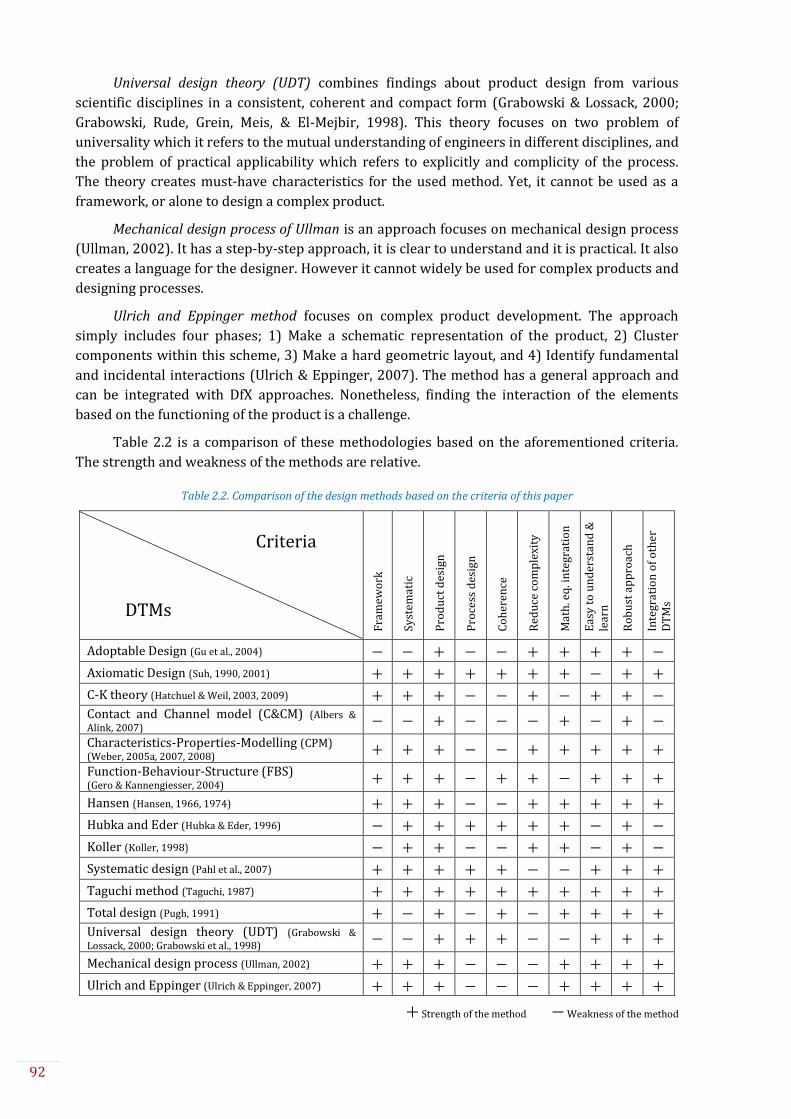
92
Universal design theory (UDT) combines findings about product design from various
scientific disciplines in a consistent, coherent and compact form (Grabowski & Lossack, 2000;
Grabowski, Rude, Grein, Meis, & El-Mejbir, 1998). This theory focuses on two problem of
universality which it refers to the mutual understanding of engineers in different disciplines, and
the problem of practical applicability which refers to explicitly and complicity of the process.
The theory creates must-have characteristics for the used method. Yet, it cannot be used as a
framework, or alone to design a complex product.
Mechanical design process of Ullman is an approach focuses on mechanical design process
(Ullman, 2002). It has a step-by-step approach, it is clear to understand and it is practical. It also
creates a language for the designer. However it cannot widely be used for complex products and
designing processes.
Ulrich and Eppinger method focuses on complex product development. The approach
simply includes four phases; 1) Make a schematic representation of the product, 2) Cluster
components within this scheme, 3) Make a hard geometric layout, and 4) Identify fundamental
and incidental interactions (Ulrich & Eppinger, 2007). The method has a general approach and
can be integrated with DfX approaches. Nonetheless, finding the interaction of the elements
based on the functioning of the product is a challenge.
Table 2.2 is a comparison of these methodologies based on the aforementioned criteria.
The strength and weakness of the methods are relative.
Table 2.2. Comparison of the design methods based on the criteria of this paper
Criteria
DTMs
Fra
mew
ork
Syst
emat
ic
Pro
du
ct d
esig
n
Pro
cess
des
ign
Co
her
ence
Red
uce
co
mp
lexi
ty
Mat
h. e
q. i
nte
grat
ion
Eas
y t
o u
nd
erst
and
&
lear
n
Ro
bu
st a
pp
roac
h
Inte
grat
ion
of
oth
er
DT
Ms
Adoptable Design (Gu et al., 2004) Axiomatic Design (Suh, 1990, 2001) C-K theory (Hatchuel & Weil, 2003, 2009) Contact and Channel model (C&CM) (Albers & Alink, 2007) Characteristics-Properties-Modelling (CPM) (Weber, 2005a, 2007, 2008) Function-Behaviour-Structure (FBS) (Gero & Kannengiesser, 2004)
Hansen (Hansen, 1966, 1974) Hubka and Eder (Hubka & Eder, 1996) Koller (Koller, 1998) Systematic design (Pahl et al., 2007) Taguchi method (Taguchi, 1987) Total design (Pugh, 1991) Universal design theory (UDT) (Grabowski & Lossack, 2000; Grabowski et al., 1998)
Mechanical design process (Ullman, 2002) Ulrich and Eppinger (Ulrich & Eppinger, 2007)
Strength of the method Weakness of the method

93
From this list, Axiomatic design, FBS and CPM are chosen as the candidates to create an
approach for managing complexity in concurrent designing. Axiomatic design is chosen due to
its systematic framework and creation of a link between function and structure of a system. FBS
and CPM are considered due to their modelling capabilities for product development and the
fact that they can integrate other design methods. These three candidates are explained in the
following sub-sections.
2.5.2. Axiomatic Design (AD)
Axiomatic design is a common theory which is introduced by Suh in 1990. Its goal is “to
establish a scientific basis to improve design activities by providing the designer with a theoretical
foundation based on logical and rational thought process and tools” (Suh 1990). According to the
Axiomatic design, design involves interplay between “what we want to achieve” and “how we
choose to satisfy the need”. The design world consists of four domains: customer domain,
functional domain, physical domain and process domain (Figure 2.9). Every domain maps the
domain on the right side which aims to satisfy the requirements of the left column (Suh, 2001).
Functional
Requirement
(FR)
Customer
Attributes
Design
Parameters
(DP)
Process
Variables
Mapping MappingMapping
Customer
Domain
Functional
Domain
Physical
Domain
Process
Domain
Figure 2.9. Axiomatic Design (Suh, 2001)
The customer domain is characterises by customer needs. In functional domain, customer
needs are specified in form of functional requirements (FR) and constraints. In physical domain,
design parameters (DP) are chosen to satisfy the functional requirements. Finally in process
domain, the process variables are specified based on DPs.
From product design point of view, Figure 2.9 will be customized as Figure 2.10. So the FR,
as “what we want to achieve”, is engineering specifications which is being satisfied by the design
parameters. The uncertainty in determinations of the design parameters creates complexity of
satisfying the required accuracy and tolerance.
Engineering
Specifications
Customer
Requirements
The key Design
Parameters
Manufacturing
Process
Variables
Mapping MappingMapping
Customer
Domain
Functional
Domain
Physical
Domain
Process
Domain
Figure 2.10. Axiomatic Design Method in Product Design (Suh, 2001)
In axiomatic design there two major axioms:
1) Independence axiom: Maintain the independence of the functional requirement.
In mapping between FRs and DPs, each FR should be able to be satisfied without
affecting other FRs.
2) Information axiom: Minimize the information content of the design.

94
If there is more than one design that satisfies the same FRs and confirms the
independence axiom, the best one is the one with minimum information content.
Axiomatic design can be used in concurrent designing. The relationship between physical
domain and process domain create links between product and process. Therefore, the
manufacturing process variables are specified by the key design parameters. Moreover, in
creating the structure model, there is a zigzag between functional and physical domain as it is
shown in Figure 2.11. The decomposition of a system is done in two functional and physical
domains in parallel. The study starts from the highest level of conceptual design where there is
enough information about the required function of a system. Then, from an FR in functional
domain we conceptualize the design and determine the corresponding DP in physical domain.
Then we go back to functional domain and decompose FR into two FR1 and FR2 that collectively
satisfies FR. This zigzag approach continues until the FR can be satisfied without further
decomposition (Suh, 2001). This approach is used as the base on the proposed approach of this
thesis. The detail of the approach is explained in chapter 3.
FR
FR1 FR2
FR11 FR12
FR122FR121 FR123
FR1231 FR1232
DP
DP1 DP2
DP11 DP12
DP122DP121 DP123
DP1231 DP1232
Functional Domain Physical Domain
Mapping
Decom
positio
n
Figure 2.11. Zigzagging approach in axiomatic design (Suh, 2001)
2.5.3. Function-Behaviour-Structure (FBS)
Function-Behaviour-Structure (FBS) which first introduced by Gero (1990) is a method to
model a system based on its function, behaviour and structure. Function is defined as an
intermediate between the needs and the behaviour of a system. Behaviour describes the
attributes that are derived (or expected to be derived) from the structure. Structure is the
components of the system and their relationships. There are eight processes in FBS framework
as shown in Figure 2.12.
Figure 2.12. The FBS framework (Gero, 1990)
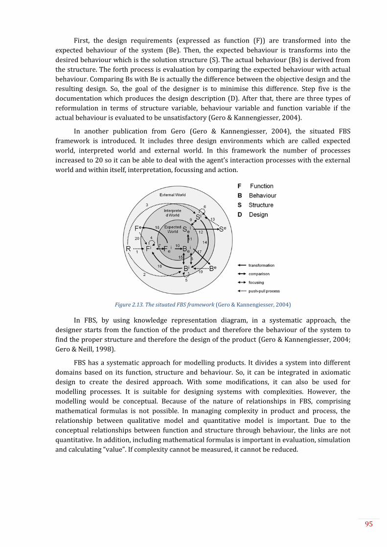
95
First, the design requirements (expressed as function (F)) are transformed into the
expected behaviour of the system (Be). Then, the expected behaviour is transforms into the
desired behaviour which is the solution structure (S). The actual behaviour (Bs) is derived from
the structure. The forth process is evaluation by comparing the expected behaviour with actual
behaviour. Comparing Bs with Be is actually the difference between the objective design and the
resulting design. So, the goal of the designer is to minimise this difference. Step five is the
documentation which produces the design description (D). After that, there are three types of
reformulation in terms of structure variable, behaviour variable and function variable if the
actual behaviour is evaluated to be unsatisfactory (Gero & Kannengiesser, 2004).
In another publication from Gero (Gero & Kannengiesser, 2004), the situated FBS
framework is introduced. It includes three design environments which are called expected
world, interpreted world and external world. In this framework the number of processes
increased to 20 so it can be able to deal with the agent’s interaction processes with the external
world and within itself, interpretation, focussing and action.
Figure 2.13. The situated FBS framework (Gero & Kannengiesser, 2004)
In FBS, by using knowledge representation diagram, in a systematic approach, the
designer starts from the function of the product and therefore the behaviour of the system to
find the proper structure and therefore the design of the product (Gero & Kannengiesser, 2004;
Gero & Neill, 1998).
FBS has a systematic approach for modelling products. It divides a system into different
domains based on its function, structure and behaviour. So, it can be integrated in axiomatic
design to create the desired approach. With some modifications, it can also be used for
modelling processes. It is suitable for designing systems with complexities. However, the
modelling would be conceptual. Because of the nature of relationships in FBS, comprising
mathematical formulas is not possible. In managing complexity in product and process, the
relationship between qualitative model and quantitative model is important. Due to the
conceptual relationships between function and structure through behaviour, the links are not
quantitative. In addition, including mathematical formulas is important in evaluation, simulation
and calculating “value”. If complexity cannot be measured, it cannot be reduced.

96
2.5.4. Characteristics-Properties Modelling
About ten years ago Weber developed an approach called Characteristic-Property
Modelling (CPM) for product/system modelling and respectively Property-Driven Development
(PDD) to explain the process of developing and designing the products (Weber et al., 2003;
Weber, 2009).
The concept of CPM/PDD is mainly based on the distinction between “characteristics” and
“properties” of a product or proces. (Tomiyama et al., 2009; Weber et al., 2003).
Characteristics (Ci) are the parameters that can be directly influenced or determined by
the designer. For instance: shape, structure, dimension, Bill of material (BOM), material
and surface of the product.
Properties (Pj) are the product behaviour, which means, the parameters that the designer
cannot change directly but they can be changed indirectly by means of the
characteristics. For instance: function, weight, aesthetic properties, safety and reliability,
cost, manufacturability.
Required Properties (RPj) are the parameters that the designer/customer is desired to
achieve.
Characteristics are also called “internal properties” or “design parameters” in other
methods, and properties are also called “external properties” or “functional requirements”
(Hubka and Eder, 1996; Suh, 1990).
Dependencies (Dij) are between the characteristics which could be geometrical, spatial, or
material.
Relations (Rj) represent the interrelation between characteristics and properties.
The relations correspond with two main activities; analysis and synthesis.
Analysis; Based on known/given characteristics of a product its properties are
determined or, if the product does not yet exist in reality, predicted. Analyses can, in
principle, be performed experimentally or ‘virtually’ (e.g. using digital simulation tools).
Synthesis; Based on given/required properties, the product’s characteristics are to be
determined. The development/design process begins with a list of required properties.
The designer’s task is to find appropriate solution patterns and determine/assign their
respective characteristics in such a way that the required properties are met to the
customer’s satisfaction (Weber et al., 2003).
In addition to the characteristics and properties, there are other parameters that influence
on the system. These parameters are called External Conditions (ECk). According to (Weber,
2007): “The determination/prediction of every product property via an appropriate model, method
and tool must be performed with respect to these parameters”.
For a more straight-forward definition of ECk, we defined it as;
External Conditions (ECk) are the parameters that the designer cannot change directly
and uniquely, and also they cannot be changed indirectly by modification of the
characteristics. In other words, external conditions are defined by external environment
in which the designer doesn’t have control over.
Another element that needs clarification is “Modelling Condition”.

97
Modelling Conditions (MCn) are “the set of assumptions, hypothesis, boundary conditions or
simplifications used while developing the model that have to be taken into account for
defining the relations between the characteristics and the properties” (Dantan et al., 2013).
PDD, the method for process modelling, describe the development of the product by using
analysis, synthesis and evaluation steps. Generally the process starts with the list of
requirements (RPj). The first synthesis step is to define the characteristics (Ci) based on the
requirements. The next step is to analyse the characteristics which results in properties (Pj).
Then is the evaluation step in which ∆P is created by comparing the RP with P. This was the first
cycle and then loop by loop the product gets more into detail (Figure 2.14). External Conditions
(ECk) have great influence on both synthesis and analysis.
Figure 2.14. CPM/PDD representation extracted from (Köhler, Conrad, Wanke, & Weber, 2008; Weber, 2007)
Thus, according to Weber (2007) the major four steps are;
1. The process starts with a list of requirements (RPj). The designer establishes the first
major characteristics (Ci) by some of the required properties. In practice, in this step,
partial solution is known from previous designs.
2. In the second step, the properties of current solution (Pj), based on the established
characteristics, are analysed. In this step, all the relevant characteristics in addition to
the synthesized characteristics from step 1 are considered.
3. In the third step, the result of the analysis in step 2 is used to determine the deviation of
the individual properties against the required properties. This deviation (ΔPj)
determines the shortcoming of the current design.
4. The fourth step is the overall evaluation. In this step, the main problems are extracted
and it is decided to how to proceed. The most appropriate property(/ies) with ΔPj≠0 one
by one is(are) chosen, the subsequence appropriate methods and tools are selected, and
the cycle is repeated. This cycle continues until ΔPj is fairly small.
This process terminates when all characteristics are assigned and all properties can be
determined/predicted, and also when ∆P→0 with sufficient safety and accuracy.
There are several tools to support analysis and synthesis in this model. For analysis; the
existed engineering methods and tools are; guesswork, estimation, experience, customer
interrogation, test and experiments, calculation/simulations. For synthesis; human genius,
association (technical patterns, pattern in nature), experience, standard/catalogue solutions,
C1
C2
C3
Cm
R1
R2
R3
P1
P2
Pn
RP1
RP2
RPn
Synthesis
Analysis
EC
.
.
.
MC
ΔP
ΔP
ΔPDep
end
enci
es

98
collection of rules, methodical approaches, inverted calculations and computer tools (fuzzy,
case-based reasoning etc.) are the existed engineering methods and tools (Weber et al., 2003).
CPM/PDD method is also part of Theory of Technical Systems (TTS) but the significance of
Weber’s model in compared with other methods is its process modelling approach. In other
words, the TTS approach can be completely separated from design methodology side. In
addition, the approach is a convenient base for computer-based modelling (Weber, 2005c,
2009).
CPM creates a unique language to design a robust product. Methods such as concurrent
designing and integrated product development of Andreasen (1987) can be integrated later to
this framework. Integrated product development considers three aspects of product, process
and market (Andreasen et al., 1996; Andreasen, 1987, 1994). So, it is a proper method for
concurrent designing.
CPM/PDD is in one of the DTMs in the category of general concrete methods (Tomiyama et
al., 2009). It has a general and systematic approach and it is suitable for embodiment design
phase. It gives a framework into which other DTM approaches such as Axiomatic design as well
as Pahl and Beitz (Pahl et al., 2007; Pahl & Beitz, 1996) and Hubka and Eder (Hubka & Eder,
1987) can fit. It also gives a background to integrate other methods such as DfX. In addition, it
can explain some open design theories and it delivers a theoretical base for the development and
use of methods and tools in the development process, including CAX (Conrad et al., 2007;
Tomiyama et al., 2009). Furthermore, it works with mathematical relations and finally it is
suitable to model systems with design complexities.
Due to these advantages, it is chosen as the framework of the proposed approach to deal
with complexity in IPPD. Thanks to the possibility of mathematical formulas in CPM, it creates
links between qualitative and quantitative models. The nature of relations in CPM is precise
mathematical formulas, so it is preferred to FBS.
However, the Weber’s model (which we call it the classical CPM) has some drawbacks
while dealing with complexity in IPPD that the new proposed version in Chapter 3 is hopefully a
better version inspired by the classical CPM. In addition, CPM is introduced for product design
only. In chapter 6 it is explained how it can be used for modelling manufacturing processes as
well.
2.6. Conclusion
The global product design objective in industry is to increase “value”. In order to increase
value, it needs to be assessed. Value includes quality and cost. Quality is related to product
modelling and cost is related to process modelling. So as to take both product and process
aspects into account, the concept of concurrent design was chosen as the domain of study. This
concept, along with related subjects in literature was presented.
So, the first research question is answered on why and how concurrent designing profits
industry and how value can be assessed in this theme. However, to assess value and eventually
increase it, in the following chapters, an approach for concurrent designing will be presented
and the answer will be achieved.
Complexity was identified as the main challenge in concurrent designing. The concept of
design complexity, state of the art and different visions for complexity were summarized. As a

99
result, the main difficulty is to identify the link between “value” and “design parameters”. In
addition, complexity needs to be managed in different steps of design process.
Thus, to answer the second research question, different causes for complexity in
concurrent designing are discussed. To complete the answer, we need to find how to manage
complexity. The main source of complexity is identified as uncertainty. Furthermore, the link
between the product design elements, process design elements and product-process links, in
addition to difficulty in determining the link between function and structure are other sources of
complexity. In order to manage complexity and uncertainty an approach is needed to be
applicable in both aspects according to the aforementioned criteria. To find or create an
approach for this problem, different approaches and methodologies were reviewed.
The concept of parameters’ distinction as characteristics and properties in CPM, in
addition to the product model framework of CPM are chosen to create the model of product. One
of the weaknesses of CPM is not having a systematic approach. By using the hierarchical zigzag
approach of axiomatic design, we can create a systematic top-down approach to create the
product model in CPM. By using axiomatic design approach the system can be decomposed in
various levels.
We believe CPM has a great potential as a framework of design and yet not enough work is
done about this method. Considering the strong points of CPM, an extended version of CPM can
make it the right framework to model a system and manage complexity that is due to the
complex links and uncertainty. Moreover, although classical CPM is introduced for product
modelling, the same concept can be used to model the process of manufacturing as well. In this
way, there will be coherence between product model and process model.
So, the lack of systematic decomposition approach in CPM can be fulfilled by AD
decomposition approach. Due to the capability of CPM, integration of these two will be possible.
Yet, identifying relations in CPM would be a challenge in system with complexity. Identifying the
relations and managing uncertainties in design process requires a link between functional
domain and structural domain to assure the passage from function to structure while modelling
the system’s behaviour. In this way, complexity can be managed by identifying the link between
value and design parameters.
Our proposition is to use flow modelling which will be explained in the following chapters.
In the next chapter, an approach is proposed for modelling mechanical systems by using AD, an
extended version of CPM, and energy flow modelling. In chapter 6, the approach of chapter 3 will
be developed further by using process flows to model integrated product and process system, to
help to manage complexity and therefore increase the value.

100
CHAPTER 3
1) LR: Concurrent design
2) LR: Complexity
3) LR: DTMs
4) Choosing the best
5) Creation of the Product design approach
6) Repetition of step 3 and 4.
7) Experimentation: Product design approach
8) Experimentation: Product design approach on another case study
9) Improvement of the product design approach
10) Concurrent design approach
11) Experimentation: Concurrent design approach
12) Modification on the product approach for concurrent design.
13) Sensitivity analysis
14) Uncertainty management
15) Tolerance optimisation
16) Conclusion
6. IPPM
5. Uncertainty & Complexity management
4. Case study
3. Product
2. Literature Review
1. Introduction
1.1. Context
1.2. Research questions
1.3. Research objectives
1.4. Methodology
1.5. Thesis outline
2.1. Context
2.2. Value
2.3. Concurrent designing
2.4. Complexity
2.5. DTM
3.1. Context
3.2. Extended-CPM
3.3. Energy flow modelling
3.4. Product modelling approach
3.5. Mini case study
4.1. Oil pump
4.2. Product model
4.3. Complementary tools
5.1. Uncertainty management
5.2. Sensitivity analysis
5.3. Tolerance analysis
6.1. Context
6.2. Flows
6.3. CPM in IPPD
6.4. IPPM approach
6.5. Case study
6.6. Tolerance optimisation
Research questions
1. How concurrent designing can profit industry and how to assess value in this concept?
2. What are the sources of complexity in IPPD and how to manage them?
3. How to manage design uncertainty?
4. How to model an integrated product/process system systematically to increase �value ?
5. How the model can be used to analyse and optimise the system?
M e t h o d o l o g y
Conclusion

101
CHAPTER 3:
A Proposition for Product Modelling
This chapter is the proposition of this thesis for modelling a mechanical product and guiding the designer in decision making while creating a structure based on the required function. This approach then will be extended in chapter 6 for modelling a concurrent system. The framework of the approach is based on CPM. As discussed in chapter 2, CPM is chosen because of its advantages. However, there are drawbacks in CPM for modelling systems with complexity. So, some modifications in CPM are required to be used in the approach for modelling complex systems. As here denoted an extended version of CPM, we use the elements of CPM and the framework for system’s model. However, the model is created in a systematic top-down approach. This is a zigzag approach between functional domain and structural domain. This approach is similar to zigzagging in Axiomatic Design.
The actual modelling of the product is done based on the Energy Flow Modelling (EFM). EFM models the behaviour of the system in each level of decomposition and it assures the transition from function to structure. By using EFM in the zigzag approach the physical model of product will be determined in CPM based on the required functions.
Thus in this chapter, after an introduction of the extended version of CPM and EFM, the product modelling approach will be proposed. A short case study will be presented for understanding of the approach. Another case will be studied in the next chapter in detail.

102
3.1. Context
The global design objective is to increase value. In IPPD, product and process aspects are
related to quality and cost respectively. In order to manage complexity in IPPD we focused on
the link between the elements of product and process through the design process. So, the
designer needs a methodology that identifies these links while considering design uncertainty.
In addition to the links between two aspects, the links in the product model itself should be
identified. The main link is between the function of the product and its structure. Function of a
system is to assure the desired output. So, the structure of a system must be designed based on
the function to assure the desired output.
In a complex system, identifying the link between function and structure is not straight
forward. Moreover, the identification is mostly qualitative which makes it difficult to use in
detail design phase. So, a quantitative model that is created by the transition from function to
structure is required. Then, this model can be used to analyse the system and increase the
knowledge of the designer toward the system. So, the result can be used for conceptual and
embodiment design phase.
In order to create such a model, an approach is needed to help the designer through the
modelling and design process. The approach needs to be systematic to model a system in multi
levels. So, in this chapter, we are going to propose such an approach for product design.
Other than having such hierarchical approach, both aspects function and structure should
be assured in each level of decomposition. So, a zigzag approach between two domains of
functional and structural is required.
After the literature review on different DTMs in chapter 2, CPM is chosen as the
framework of the approach. As discussed in chapter 2, CPM/PDD is capable of creating a
quantitative model of the product. The weaknesses of classical CPM are the lack of a systematic
approach and difficulty in identifying the relationships (Rij).
Therefore, an extended version of CPM is proposed in the next section. In this version,
other than differences such as having several levels of properties that is useful for complicated
systems, more importantly, it is systematic. This systematic approach is achieved by a
hierarchical approach while zigzagging between function and structure. The zigzag approach in
axiomatic design is used here. So, it gives the designer a step-by-step approach to follow.
However, in addition to this framework, we need a model to assure the quantitative link
between function and structure. The model should be based on the behaviour of the system. The
answer to this problem is discussed in section 3.3.
3.2. An extended version of CPM
In chapter 2, the classical CPM/PDD, as Weber has published, was described. In PDD, the
model of product is created by a synthesis-analysis cycle in CPM. Since Weber’s proposition,
several articles, mostly by involving the creator, have been published. A number of them present
the general concept of CPM (Conrad, Köhler, Wanke, & Weber, 2008; Weber, 2005a, 2008) while
other articles are about different aspects of CPM (Köhler et al., 2008; Qureshi, Eisenbart, Dantan,
& Blessing, 2011; Weber, 2007). CPM is a suitable framework for transition from embodiment
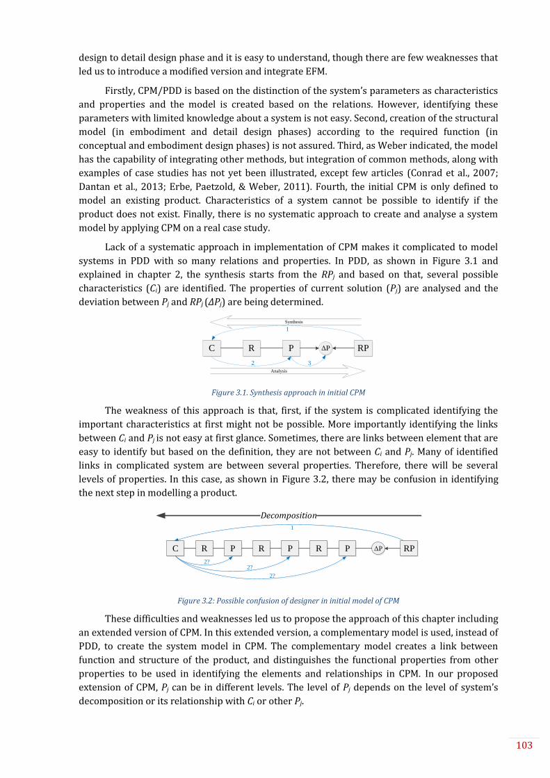
103
design to detail design phase and it is easy to understand, though there are few weaknesses that
led us to introduce a modified version and integrate EFM.
Firstly, CPM/PDD is based on the distinction of the system’s parameters as characteristics
and properties and the model is created based on the relations. However, identifying these
parameters with limited knowledge about a system is not easy. Second, creation of the structural
model (in embodiment and detail design phases) according to the required function (in
conceptual and embodiment design phases) is not assured. Third, as Weber indicated, the model
has the capability of integrating other methods, but integration of common methods, along with
examples of case studies has not yet been illustrated, except few articles (Conrad et al., 2007;
Dantan et al., 2013; Erbe, Paetzold, & Weber, 2011). Fourth, the initial CPM is only defined to
model an existing product. Characteristics of a system cannot be possible to identify if the
product does not exist. Finally, there is no systematic approach to create and analyse a system
model by applying CPM on a real case study.
Lack of a systematic approach in implementation of CPM makes it complicated to model
systems in PDD with so many relations and properties. In PDD, as shown in Figure 3.1 and
explained in chapter 2, the synthesis starts from the RPj and based on that, several possible
characteristics (Ci) are identified. The properties of current solution (Pj) are analysed and the
deviation between Pj and RPj (ΔPj) are being determined.
Figure 3.1. Synthesis approach in initial CPM
The weakness of this approach is that, first, if the system is complicated identifying the
important characteristics at first might not be possible. More importantly identifying the links
between Ci and Pj is not easy at first glance. Sometimes, there are links between element that are
easy to identify but based on the definition, they are not between Ci and Pj. Many of identified
links in complicated system are between several properties. Therefore, there will be several
levels of properties. In this case, as shown in Figure 3.2, there may be confusion in identifying
the next step in modelling a product.
C R P RPΔPPR
1
2?
R P
2?2?
Decomposition
Figure 3.2: Possible confusion of designer in initial model of CPM
These difficulties and weaknesses led us to propose the approach of this chapter including
an extended version of CPM. In this extended version, a complementary model is used, instead of
PDD, to create the system model in CPM. The complementary model creates a link between
function and structure of the product, and distinguishes the functional properties from other
properties to be used in identifying the elements and relationships in CPM. In our proposed
extension of CPM, Pj can be in different levels. The level of Pj depends on the level of system’s
decomposition or its relationship with Ci or other Pj.
C R P RPΔP
1
2 3
Analysis
Synthesis

104
Unlike PDD, our proposed approach uses a hierarchical method to identify the elements of
CPM. In this version, similar to PDD, the approach starts with RPj. According to RPj the as-is
property (Pj) is identified. Then, the system is decomposed. The decomposition is done in two
domains in parallel: the functional domain and the physical domain. By zigzagging between
these two domains the model is created. This zigzagging approach is similar to the approach of
Axiomatic Design as explained in chapter 2 (Figure 3.3).
FR
FR1 FR2
FR11 FR12
FR122FR121 FR123
FR1231 FR1232
DP
DP1 DP2
DP11 DP12
DP122DP121 DP123
DP1231 DP1232
Functional Domain Physical Domain
Deco
mp
ositio
n
Figure 3.3. Zigzagging approach in axiomatic design (Suh, 2001)
The study starts from the highest level of conceptual design where there is enough
information about the required function of the system. Then, from an FR (Functional
Requirement) in functional domain we conceptualise the design and determine the
corresponding DP (Design Parameter) in the physical domain. Then we go back to functional
domain and decompose FR into two FR1 and FR2 that collectively satisfies FR. This zigzag
approach continues until the FR can be satisfied without further decomposition (Suh, 2001). As
mentioned before, FR is the same as Pj and DP is the same as Ci. However, the definition of
function in axiomatic design and CPM are not the same. Here, function is only those properties
that transform given inputs into required outputs.
So, the designer starts with Required Properties (RPj) similar to FR. Based on that, the as-
is-properties (Pj) are identified (Similar to DP). By zigzagging between functional and structural
domain the system is decomposed and important parameters are identified. When there is no
further decomposition, the identified elements in physical domain are controllable by the
designer. So, based on the definition they are considered as Ci. All the identified parameters after
the first level and before the final level of decomposition are called “Intermediary Properties”
(IPj). So;
Intermediary properties are those parameters that cannot be categorised with
characteristics or external conditions based on the definition. They are properties but differ
from as-is-properties. They are used to decompose the as-is-properties and find/represent the
related characteristics of a property in a complex system while decomposing the system. So, they
are the intermediary parameters between the as-is-properties and characteristics.
During the zigzag approach between two domains, by using the identified parameters in
each level of decomposition, CPM is built step by step. A general construction approach of
product model using the extended version of CPM is shown in Figure 3.4. In this case, in each
level of decomposition, the properties of the current level (sub-system) are identified and the
effective parameters are identified as well. Unlike the publications of Weber, the model in our
approach is constructed from left to right. It is only for later integration of CPM in our proposed
approach. The approach will be presented in section 3.4.

105
Figure 3.4: An extended version of CPM
In a complex system, identifying the characteristics at first is not always possible. This
hierarchical decomposition of the required function helps the designer to decompose the design
problem into smaller sub-problems.
Thus, actually the use of Weber’s methodology as called CPM/PDD in our approach is
limited to CPM elements. Synthesis approach is used in a more systematic way to create the
model of product. Analysis approach is used as the second phase to utilise the created model of
product to analyse the system. So, the following concepts are utilized from CPM/PDD:
The concept of identifying the parameters as characteristics and properties,
The synthesis approach to start from required properties, properties and arrive to
characteristics,
The analysis approach to analyse the impact of effective parameters on the system’s
output.
As previously explained, a function-behaviour-structure approach with integrating
quantitative models is needed for two phases of conceptual and embodiment design as well as
the link between them. So CPM needs a complementary model to use in such approach. Lutters
et al. (2014) gathered standard tools and techniques for product design. There are several tools
that can be integrated in CPM for various purposes. Quality Function Deployment (QFD) is one of
them. The concept is to involve the competitors and customer satisfaction in the process of
design (Mizuno & Akao, 1993). Failure Mode and Effect Analysis (FMEA) and reliability
engineering plan are tools for risk analysis and reliability analysis of the product during the
functioning of the product (McDermott, Mikulak, & Beauregard, 1996). In addition, the Design
Structure Matrix (DSM) is another tool to manage complexity by concentration on information
flow and interdependencies within and between different domains (Browning, 2001; Pektas &
Pultar, 2006). These tools, considering their specific capabilities in different aspects, are not
suitable for the goal of this study as mentioned. We are looking for a general tool to be applicable
in conceptual and embodiment design in order to include both functional and structural aspects.
To extract the physical laws in order to determine the quantitative model, we propose energy
flow model to use in both functional and physical domains.
3.3. Energy flow modelling
The proposed framework by using CPM and AD creates a top-down decomposition
approach to model a system. This framework is to create a link between the identified
parameters of the system. In a complex system, identifying these parameters is not easy due to
the coupling and existence of the parameters in various levels of decomposition. The parameters
RP2
P1
P2
RRP1
IP1
IP2
IP3
R
IP4
IP5
IP9
.
.
.
R
R
EC2
R
C1
.
.
.
C2
Cn
R
R
R
C3.
.
.
EC1
MC1
MC2
EC3RP2
P1
P2
RP1
RP2
P1
P2
RRP1
IP1
IP2
IP3
R
EC1
MC1
Model SynthesisModel Synthesis
Analysis

106
can be related to the function, behaviour or structure of the product. They can also be related to
the environment of the system.
So, a model is required to be used in this framework to identify the important parameters.
In addition, the link between these parameters should be determined to identify the relations in
CPM. The model should represent functional, behavioural and structural points of view at each
step of design process. Since we are looking for a link between the functioning of the product
and its physical entities (structure), physical flow analysis can highlight this link. There exist
different flows in a product. So, in the first sub-section, product flows are studied to find the best
flow to model a system and identify the parameters and their links.
3.3.1. Product flows
In IPPD, there are different flows for product and process. In modelling a system, the
relationships between the elements of design should be established. Process flows, and how they
can be used to model a system will be discussed in chapter 6. Product flows, that can be used to
identify the link between the components, are discussed here.
In general, the function of a system can be defined as the transformation of one basic
element into another within an artefact. These elements which could be material, energy or
signal, can express the function in different levels to decompose the system (Henderson & Taylor
1993). So, among the product flows, there are three types of flows that can be used to create
links between components and identify Rm in CPM: material flow, information flow and energy
flow.
Material flow is the flow of solid, liquid or gas material through the system. In process
design, it can be also the flow of product parts, which it is one of the best means for designing
manufacturing processes. In product design, if transferring material is the main purpose of the
product, it can be used to model it. However, in most cases with only considering material flow,
many aspect of the product might be ignored.
Information flow is mostly used in system engineering or processes. One of the known
information models is System Integration of Manufacturing Applications (SIMA) that has been
launched by the National Institute of Standards and Technology (NIST) to address the
information interface needs of the U.S. manufacturing community (Y. T. Lee, 1999; McLean &
Leong, 1995). This type of flow is also a good means in process design. For product design, it can
be used for control planning such as monitoring or maintenance. It can also be used for process
feedback for quality control. Yet, it cannot be used to identify the physical links between the
components that are important in functioning of the product.
Energy flow is the passage or transformation of energy in a system. It also considers the
consumption of energy. For modelling mechanical products, energy flow is one of the best means
to find the physical links between the elements (Pailhès et al., 2007). This is the case when the
energy flows are the functional flows of the system. In this case, energy flow can be used to
model the behaviour of the system and identify the links.
Thus, in this point of view, functioning of a product can be defined as having the flows of
product as smooth as possible. Analysis of the flow gives us the direction of the development as
well as how the functioning of the different parts of the product is related to each other. In other
words, we can evaluate the product function according to the flows of energies. This evaluation
can be done in different levels of decomposition using flows in different levels.

107
Energy in a system can be transferred or/and transformed. There are four types of energy
transformation; emission of energy (e.g. expansion of a compressed gas), energy flux
transformation by a certain program (e.g. pressure transfer in a liquid or polarization of light),
conversion of energy (e.g. transformation of mechanical energy into hydraulic energy), and
absorption of energy (e.g. deformation or gas compression) (Savransky, 2000). This type of flow
is used for modelling the behaviour of a system in this thesis.
There are several energy flow modelling approaches in literature. The criteria for choosing
the best EFM is that it should be able to integrate in extended-CPM. Secondly, it needs to create a
link between function and structure. Thirdly, the created model by the methodology should be
based on the system’s behaviour. Finally, it helps the designer to identify the effective
parameters.
Bond graph (Paynter, 1961) is one of the EFMs that can be integrated in CPM. As
(Borutzky, 2010) stated, “bond graph modelling starts from the intuitive and physical approach
that a dynamic system is composed of subsystems, components, or basic elements that interact by
exchanging energy”. So, it can create the link between function and structure. However, bond
graphs represent the physical structure of a system. So, without enough knowledge about the
structure of a system, bond graph is not effective.
Internal Block Diagram (IBD) is one of the models in SysML (Friedenthal et al., 2012) that
also represents the structure of a system. IBD is mostly used for modelling signal flow in system
engineering. However, as represented by (Albers & Zingel, 2013) it can be used for mechanical
design as well. SysML is a combination of various diagrams. For the purpose of our research,
parametric diagram can be used for representation of the links between the parameters. With
activity diagram, the behaviour of the system can be modelled. So, a combination of SysML
diagrams can represent the parameters, links, structure and behaviour of a system.
Nevertheless, like bond graphs, IBD is based on a known structure of a system and they cannot
be used for modelling a non-existing product. In addition, parametric model considers the
element of a system as parameters without distinction between Ci and Pj or between functional
parameters and physical parameters. Moreover, in any of SysML models the notion of modelling
condition (MCn) does not exist.
Another EFM is Four-pole/Mutli-pole theory (Oppelt, 1972) that also can be integrated in
CPM (Weber, 2005b). This theory is known mostly in electrical, control and acoustics. It
describes the dynamic behaviour of a system that transmits power (Oppelt, 1972). So, this
theory focuses on modelling the behaviour of a system. We are looking for a model that create a
link between function and structure. After identifying the required structure to satisfy the
desired function, models such as IBD or Bond graphs can be used for structural modelling.
CTOC is another EFM that is created by (Pailhès et al., 2007) and it can interoperate with
extended-CPM in order to satisfy the abovementioned criteria. CTOC focuses on the minimum
structural requirement of a system to satisfy the needs. So, instead of considering all the flows
(like in Bond Graph, IBD or Four-pole/Multi-pole Models), it focuses on the flows that are
necessary to achieve the required function. Since the analysis is based on the functional
requirement, in modelling by CTOC, the structure is not necessarily known but rather the
structure can be built based on the functional requirements. So, unlike other aforementioned
models, it can be used before knowing the description of a system. In the following sections, it is
shown how CTOC in our approach can help the designer to assure the transition from function to
structure.

108
3.3.2. CTOC: An energy flow model
One of the energy flow models is the one proposed by Pailhès (Pailhès et al., 2007; Pailhès,
Sallaou, Nadeau, & Fadel, 2011; Pailhès, 2013). This model, which is also called CTOC (Converter,
Transmitter, Operator, Control), is based on the design theory of TRIZ (Altshuller, 1984, 1999).
TRIZ or ‘Theory of invention problem solving’ contains a set of tools and methodologies for
generating inventive solutions for design problems. One of the eight “laws” of technology
evolution in TRIZ is the “law of completeness of system parts” (Altshuller, 2008; Savransky,
2000). This law, which decomposes the system into specific entities, focuses on the minimum
requirements to describe a system.
Design problems can be divided into routine and non-routine problems. A problem is
routine if all critical steps to a solution are known. A problem is non-routine if at least one of the
critical steps is unknown. Non-routine problems need inventive problem solving method. Major
problems in design and development are inventive. TRIZ is a noble method for inventive
problem solving in conceptual design. So CTOC, which is based on TRIZ, is used in our approach
for managing design problems by modelling the behaviour of a system and find the relations in
CPM.
According to CTOC, which models a system based on the energy flow, a system could
consist of;
Convertor (C): It converts the input energy into another type of energy to be used by
other components of the system.
Transmitter (T): It transmits the received energy without changing the type of energy.
Operator (O): It fulfils the required action depends on area of operation. According to
design situation, the operator can be a transmitter or a convertor.
Control (C): It insures that different components perform correctly.
Reference: It insures maintaining the position of different elements (Convertor and
transmitter) to support smooth passage of energy flow.
Each component is defined based on its functioning regarding the input/output type of
energy. According to that, the flow might be provided, stored, converted or transmitted. In case
of providing or storing function, the conversion of energy is the conversion of external energy
into potential internal energy and vice versa. For example, while storing water in a water tower,
the hydraulic energy is being converted into potential energy of water. Table 3.1 shows which
class of function to choose based on the input and output energy type.
Table 3.1. Classes of function in CTOC
Function Input energy Output energy
Transmit Energy type 1 Energy type 1
Convert Energy type 1 Energy type 2
Convert/provide No input Energy
Convert/store Energy No output
As Table 3.1 shows, in CTOC other than conversion and transmission, the elements of
resistance and capacity can be modelled too. So, these two elements in addition to inertia are
inside “C”. As table 3.1 shows, in CTOC the function of the entity is important. So, depends on the

109
functionality, one component can be at one point an energy storage while in another point in the
process is used to provide the energy. Compared to other energy flow models, in CTOC the
functionality is important.
The function of the interaction components is to connect the components together and to
allow the energy to pass smoothly. The inevitable losses have to be reduced or eliminated by the
designer. Managing these interactions is important in structural point of view since not only it
allows creative designs, but can also generate a logical hierarchy of solutions. A general
structural model of a system based on CTOC is shown in Figure 3.5.
Figure 3.5: General structural model of a system according to CTOC
So, the main element of CTOC is Operator. Operator is based on the desired output of the
system. For instance, if the main function of the system is conversion, operator is a convertor.
Other elements are defined based on the required input of operator. If the input energy of the
system needs to be converted to enter Operator, a convertor is required. If the input energy
needs to be transmitted from an area to Operator a transmitter is required.
In this model, “Reference” is related to the design process. It can be the ground that the
system is placed, or hand if the user holds the device. So it can be an internal or external to the
system. Interaction component (shown as small circles in Figure 3.5) connects different
components and the reference of the system. This model is used in this study to identify the
relationship of the components based on the important factor in functioning of the product
which is energy.
While modelling a system, there might be several functions to satisfy the required output
of the system. In this case, for each function there is an energy flow. For each flow a CTOC model
is required. Therefore, there will be many CTOC models as the number of functions. In this
respect, there will be common parts in the models. It is important that the models are
compatible with each other to follow the rule of satisfying the minimum requirements. For
example, if the same component can be used as transmitter in two of the models, it should not be
considered as two different components. So, it is necessary to pay attention to the links between
the CTOC models.
Function can be in different forms. In addition to the main functions as described earlier,
function can be in form of service or constraints. The same logic of CTOC as used for main
function is used for service and constraints.
This model has the same base as “physical systems theory” (PST) (Koening, Tokad, &
Kesavan, 1967). PST is initially developed to model and analyse discrete physical systems and
therefore to represent the physical relationships in a system (Sushil, Singh, & Jain, 1988; Sushil,
1991) similar to CTOC. According to Sushil (2002) there are three fundamental premises in PST:
TransmitterConverter Operator
Control
E1 E2 E2 E3
Reference
Required
Function

110
1. “Systems behaviour is primarily determined by the structure of its components and their
interrelationships.”
2. “In a discrete system (having discrete components united at a finite number of interfaces), a
component/sub-system can be modelled in isolation to characterize its behaviour as an
independent entity irrespective of its interactions with other components and the
environment.”
3. “The components of a system interact in a manner such that the principle of conservation
holds good within the system for all of its variables.”
While CTOC is based on the same principles to model the system and representing the
relationships, there are few differences. CTOC in our approach is used to support CPM and
identify its elements. Unlike PST, CTOC is not based on the representation of all flows in a system
but only the functional flows. Functional flows are those that are necessary to satisfy the
required function. So, the difference is that Unlike PST, CTOC is not searching for the flows’
description but it focuses on the minimum requirement of a system to assure the transition from
function to structure.
For better understanding of this model, the mechanism of a wind turbine is used as an
example (Figure 3.6). After need, functional and system analysis, a very important step is
physical analysis (Pailhès et al., 2007; Pailhès, 2013). Physical analysis identifies the relevant
physical behaviour of the system. The system as a black box is shown in Figure 3.6.
Figure 3.6: Wind turbine system as a black box
The objective of the system is to generate electricity. As Figure 3.6 illustrates, the main
function of a wind turbine can be also defined as “Transforming the aeraulic power of the wind
into electrical power supplied to the network”. So, the rotor receives the wind energy and
converts it into mechanical energy (Converter). By means of the gears and shaft the mechanical
energy is transferred to the generator (Transmitter). Finally the generator converts the
mechanical energy into electrical energy (Operator). The CTOC schema is shown in Figure 3.7.
Figure 3.7: CTOC model of a wind turbine (Pailhès, 2013)
The analysis of CTOC might be done in several levels of decomposition. Taking speed-
multiplier gear as an example to decompose, the major function is “Rotatively transmits the
mechanical energy”. Table 3.2 illustrates the various flows linked to its implementation. Input
shaft, gears and output shaft are the components related to this function. The induced effects
Wind turbine
Aeraulic
energy
Electrical
energyGenerate
electricity
Speed-multiplier
gearRotor Generator
Control system
C T OAeraulic
energyMechanical
energy
Electrical
energy
C
Ground
Mechanical
energyGenerate
electricity

111
result in power loss in the form of heat, distortion, wear, or noise. Therefore, other components
(housing and oil) are needed for induced effects.
Depends on the designer’s objectives, each element of CTOC is decomposed in component
level. Based on the function, energy flow and link between components, the relationship
according to physical laws can be found. If any other component of the wind turbine is
decomposable, based on the objective it can be decomposed and related equations should be
found.
Table 3.2: Components of speed-increasing gear and relative flows (Pailhès, 2013)
Component Function Functional flows Induced flows
Input shaft Rotatively transmits the mechanical energy
Mechanical energy flow
- Strain energy flow (shaft torsion)
Gears Transforms the rotational speed
Mechanical energy flow
- Thermal energy flow (contact friction, effusivity) - Strain energy flow (tooth bending, contact) - Sound energy flow - Material flow (wear)
Output shaft Rotatively transmits the mechanical energy
Mechanical energy flow
- Strain energy flow (shaft torsion)
Housing Rotatively guides the shaft
Mechanical energy flow (contact)
- Thermal energy flow (friction) - Sound energy flow - Mechanical energy flow (friction, resisting, torque) - Material flow (wear)
Oil Transports thermal energy
- Thermal energy flow - Material flow
- Mechanical energy flow (oil viscosity, resisting torque)
After this analysis, the designer will have a better knowledge on the system part by part
based on the function of that component. The related parameters will be found by the equations.
So, the importance of each component based on its functioning or in other words, its impact on
the system will be recognized. If product analysis is integrated with manufacturing process
analysis, the value-added processes can be found. Therefore, it will be very useful for cost
analysis of the product to see the distribution of cost for different components based on the
importance of that component.
CTOC highlights only the essentials to design the product. In each stage of design there
might be alternatives and the choices should be made based on different criteria. Nevertheless,
CTOC gives the designer a vision to find the essentials for the required function and therefore
lead him to a reliable solution.
Although the target of this model is systems which includes energy flows, it is applicable
on other products too. To clarify this, a “chair” is used as an example of a product without actual
energy flow. As described in (Pailhès et al., 2011), to synthesis the product based on the flow of
energy, one can identify the components of the system by virtual mechanical flow. Therefore, the
system model based on CTOC will be as Figure 3.8.
Even though, studying such systems is possible but it is not recommended to use CTOC
vision for such system. This approach is most effective when the energy flow is the basis of
functioning of the system.

112
Figure 3.8: Example of a chair in CTOC (Pailhès et al. 2011)
The model of CTOC is used in our proposed approach to model the behaviour of the
system and to assure the transition from function to structure. Its concept is used in two forms
of functional model and structural model. In functional model, the objective is to satisfy the
needs. Whether the system exist or not, the function can be divided into sub-functions. Each sub-
function is defined based on the energy flow. So, the elements of the CTOC will be Conversion,
Transmission, Operation and Control. The structural model, which is based on the functional
model, divides the system into the elements of Converter, Transmitter, Operator and Control. In
this model Reference and interaction elements should be specified. The systematic appraoch of
modelling a system by using CTOC, Axiomatic-Design-inspired zigzagging and CPM is described
in the next section. In the final level of decomposition, where the enough knowledge about the
required strucutre of the system is obtained/decided, a model like IBD or Bond graph can be
used to represent the structure of the system.
3.4. A proposed approach for product modelling
As mentioned in the first chapter, according to Pahl & Beitz (1996) there are four phases
in design: planning and task clarification, conceptual design, embodiment design and detail
design. In each phase, the potential solutions for fulfilling the needs are evaluated by comparing
them with each other and against the problem or need (Blessing & Chakrabarti, 2009). In the
embodiment design phase, a model of behaviour is required which is based on the structure of
the product. The structures are the potential solutions (concepts) as the result of the conceptual
design phase. Therefore, the required model in the conceptual design phase should not only be
able to abstract the problem and search for suitable working principles, but also be functional
and structural. Besides, during the embodiment design phase, the designer needs mathematical
models to use for pre-dimensioning and dimensioning of the product. Furthermore, such
mathematical models are useful for probabilistic sensitivity analysis and optimisation and will
be a better foundation for the detail design phase. Thus, in this section, the aim is to propose a
methodology or approach to help the designer in transition from required function to the
physical structure and therefore to create a pathway for the designer from conceptual design
phase to embodiment design phase.
Among the tools and techniques that are discussed in chapter 2, Function-Behaviour-
Structure (FBS) (Gero, 1990) is a model that can be used in both phases of conceptual and
embodiment design for the decomposition of the system. FBS identifies the elements of the
system as function, behaviour or structure. By using knowledge representation diagram, in a
systematic approach, the designer starts from the function of the product and therefore the
behaviour of the system to find the proper structure and so the design of the product (Gero &
Chair
Virtual
mechanical
energy
Maintain
the user in
position
Seat
Virtual
mechanical
energyMaintain
the user in
positionChair frame Chair legs
T T T
CTOC (Level 1)
CTOC (Level 2)

113
Kannengiesser, 2004; Gero & Neill, 1998). By using FBS, one is able to determine function and
physical behaviour of the components and therefore decompose the system.
Because of the nature of relationships in FBS, one cannot achieve a quantitative model. So,
we need another approach with advantages of FBS but also be able to use mathematical
formulas as the relations between the parameters. We are looking for an approach that is more
formalised than FBS. In FBS there is no strict separation between physical parameters and
behavioural parameters. The proposed approach of this section has a more systematic approach
for modelling products than FBS.
Thus, the proposed approach is to use CTOC in the framework of CPM in a top-down
systematic approach. The approach is composed of a multi-level modelling approach with 2
concurrent, interlinked modelling domains: functional and structural. In each level of
decomposition, CTOC is used to identify the elements of CPM to create the system model.
Therefore, the system’s structure is modelled based on the minimum requirement in order to
satisfy the needs. The result will be a model of the system including functional, behavioural and
structural descriptions of the product to be used in transition from conceptual to embodiment
design phase. The created model can also be used to analyse the impact of system’s elements on
the output of the system.
The proposition of this thesis for concurrent designing is described in chapter 5 which by
using the same concept as this section’s approach, it is extended. In this section, the product
modelling/analysis approach along with a set of rules to apply is presented.
As aforementioned, the approach includes two domains of functional and structural. In
each domain a model of system is created. So, in functional domain the functional model is
created based on the customer needs or RPj. In structural domain, the structural model is
created based on the functional model to satisfy the required function. Using the axiomatic
design, the system is decomposed level by level. Two models of functional and structural in the
related domains are created in each level of decomposition. In each model, the elements of CPM
are identified. Thanks to the energy flow, the relationships are identified as well.
3.4.1. Level 1
The approach begins with analysing the customer needs. Customer need, which has
normally a qualitative value, should be translated into quantitative value. This value in CPM
terminology is considered as required property (RPj). In order to quantify the needs, normally
increasing “value” is considered as the main objective. Since, in this thesis, we defined value as a
unit to measure both product and process, here, we call it “product value”. So, the designer
should look for parameter(s) that is (are) considered quality for the customer. Then, this
parameter becomes the product value or RPj.
The next level is to identify the required function to satisfy the need(s). So, the first model
shows the objective of the design. As Figure 3.9 illustrates, the objective is to satisfy the required
output. In this level, the system is defined as a black box while it does the required function.
For CPM, the required output is placed as RPj. This model is considered as the functional
model in level 1.
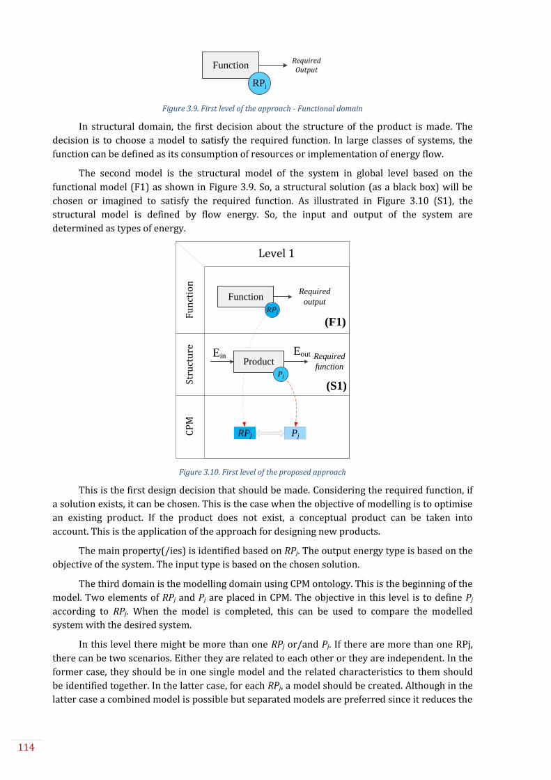
114
Figure 3.9. First level of the approach - Functional domain
In structural domain, the first decision about the structure of the product is made. The
decision is to choose a model to satisfy the required function. In large classes of systems, the
function can be defined as its consumption of resources or implementation of energy flow.
The second model is the structural model of the system in global level based on the
functional model (F1) as shown in Figure 3.9. So, a structural solution (as a black box) will be
chosen or imagined to satisfy the required function. As illustrated in Figure 3.10 (S1), the
structural model is defined by flow energy. So, the input and output of the system are
determined as types of energy.
Figure 3.10. First level of the proposed approach
This is the first design decision that should be made. Considering the required function, if
a solution exists, it can be chosen. This is the case when the objective of modelling is to optimise
an existing product. If the product does not exist, a conceptual product can be taken into
account. This is the application of the approach for designing new products.
The main property(/ies) is identified based on RPj. The output energy type is based on the
objective of the system. The input type is based on the chosen solution.
The third domain is the modelling domain using CPM ontology. This is the beginning of the
model. Two elements of RPj and Pj are placed in CPM. The objective in this level is to define Pj
according to RPj. When the model is completed, this can be used to compare the modelled
system with the desired system.
In this level there might be more than one RPj or/and Pj. If there are more than one RPj,
there can be two scenarios. Either they are related to each other or they are independent. In the
former case, they should be in one single model and the related characteristics to them should
be identified together. In the latter case, for each RPj, a model should be created. Although in the
latter case a combined model is possible but separated models are preferred since it reduces the
Function
RPj
Required Output
Fu
nct
ion
Stru
ctu
reC
PM
Level 1
PjRPj
Function
RPj
Required
output
ProductEin Eout Required
functionPj
(F1)
(S1)
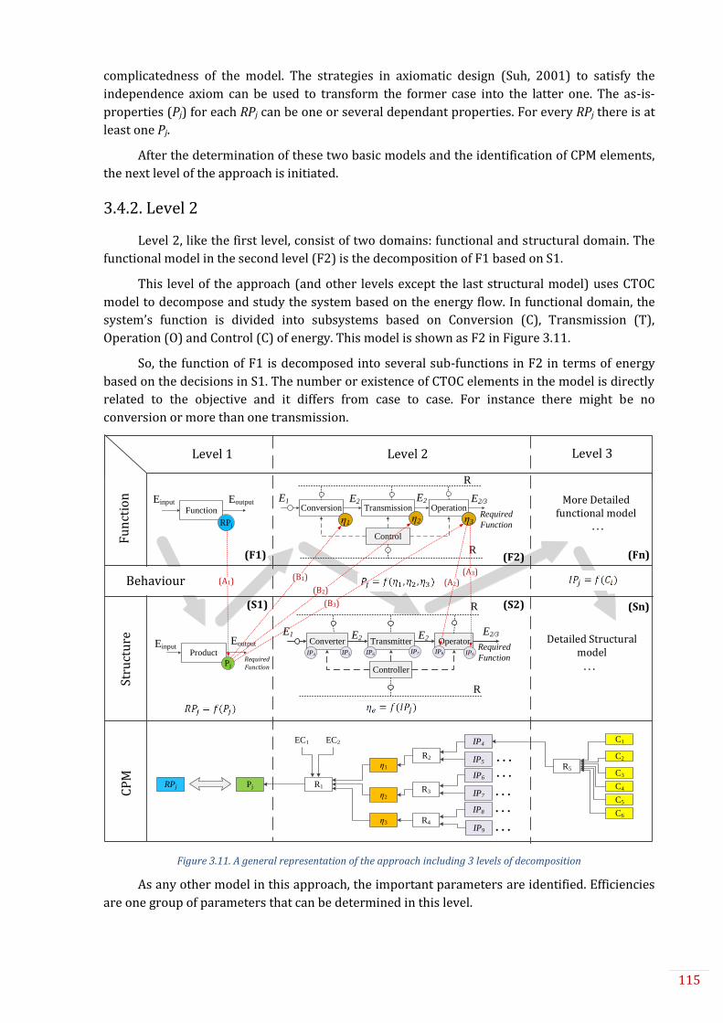
115
complicatedness of the model. The strategies in axiomatic design (Suh, 2001) to satisfy the
independence axiom can be used to transform the former case into the latter one. The as-is-
properties (Pj) for each RPj can be one or several dependant properties. For every RPj there is at
least one Pj.
After the determination of these two basic models and the identification of CPM elements,
the next level of the approach is initiated.
3.4.2. Level 2
Level 2, like the first level, consist of two domains: functional and structural domain. The
functional model in the second level (F2) is the decomposition of F1 based on S1.
This level of the approach (and other levels except the last structural model) uses CTOC
model to decompose and study the system based on the energy flow. In functional domain, the
system’s function is divided into subsystems based on Conversion (C), Transmission (T),
Operation (O) and Control (C) of energy. This model is shown as F2 in Figure 3.11.
So, the function of F1 is decomposed into several sub-functions in F2 in terms of energy
based on the decisions in S1. The number or existence of CTOC elements in the model is directly
related to the objective and it differs from case to case. For instance there might be no
conversion or more than one transmission.
RPj Pj
EC1 EC2
R1
η1
η2
η3
R2
IP4
IP8
R5
C1
C2
C3
C4
C5
C6
Fu
nct
ion
Stru
ctu
reC
PM
Behaviour
TransmissionConversion Operation
Control
E1 E2 E2 E2/3
R
η1 η2
R
Required
Functionη3
Level 1 Level 2 Level 3
Function
Einput Eoutput
RPj
Product
Pj
EinputEoutput
Required Function
TransmitterConverter Operator
Controller
E1 E2 E2E2/3
R
R
Required
FunctionIP7IP5 IP9IP4 IP6 IP8
IP5
IP6
IP7
IP9
R3
R4
�����
�
�
More Detailed functional model
Detailed Structural model
(F1)
(S1)
(F2)
(S2)
(Fn)
(Sn)
(A1) (A2)(A3)
(B1)
(B2)
(B3)
Figure 3.11. A general representation of the approach including 3 levels of decomposition
As any other model in this approach, the important parameters are identified. Efficiencies
are one group of parameters that can be determined in this level.

116
In this level or any other level of this approach, the relationship of the current level’s
parameters with the parameters of the precious level must be identified in forms of clear
mathematical formulas. The relations are between F(n) and S(n-1) (such as A1, A2 and A3) or
between Sn and Fn (such as B1, B2 and B3). So, in this level the relation is between F2 and S1. A
general representation of this relation considering efficiency (η) is as Eq. 3.1.
𝑃𝑗 = 𝑓(𝜂𝑖) (3.1)
Based on the model F2, the structural model (S2) is determined. This model is shown in
“structure” section of Figure 3.11-level 2. According to the function of each subsystem, a physical
entity or a group of entities can be chosen to satisfy the required function of the subsystem. If
such entity does not exist, it is defined. One of the best tactics is to use known solutions to satisfy
the sub-functions. Finding solutions for sub-functions is easier than for the main function. If for
any sub-function, a solution does not exist, it can be decomposed further.
To be noted, in these models, the solutions are found only for satisfying the required
function. This is due to the fact that this approach only models the minimum requirement
structure for satisfying the required function. By using the result model as a base for designing
the product, the designer can focus on their creative solutions to add.
As shown in Figure 3.11 (S2), the important parameters in this model are intermediary
properties (IPj). Although it is rare for a complex system but it is possible to identify
characteristics (Ci) too. While the IPj in this model are placed in the next column of CPM, if there
is any Ci in this level or any other level, there should be placed directly in the last column
(rightmost) of the model.
As in any other level the relations of the parameters with the previous model’s parameters
are identified. The general equation is as Eq. 3.2.
𝜂𝑖 = 𝑓(𝐼𝑃𝑗) (3.2)
It is important to remind that, this is a structural level of the model. So, each box in this
model contains a physical entity or a group of entities. This is the reason to put the general name
of elements as “converter”, “transmitter”, “operator” and “controller” while in the functional
model the elements are “conversion”, “transmission”, “operation” and “control”.
Assigning/defining components in CTOC is started from the Operator (O) as the main
element. Then, based on the received types of energy, if transmitter (T) or/and converter (C) is
needed, they will be added. Despite these elements, if an entity is responsible for controlling the
functioning of other components is named Control (C). This tactic in CTOC is applicable in both
functional and structural domains.
As indicated, in the law of TRIZ, the designer should focus on the minimum requirements
to describe the system. So, as mentioned earlier, in modelling the system based on CTOC,
dividing the system into the elements does not necessarily means having all the elements of C, T,
O and C. The element of Operator is obligatory since it contains the main function of the product.
So without this element the product would not exist. The elements of Converter and Transmitter
are not obligatory to have. In other words, a system with only the element of Operator can be a
complete system. In fact, the designer should try to achieve an ideal system with a minimum of
necessary elements. With this approach, the complexity of the system will be reduced as well.

117
The element of Control on the other side, though it is not obligatory, is desired. As
aforementioned, this element is responsible to assure the functioning of other components. So,
although a system without the element of Control can be a complete system, with this element
the result will be a more robust product.
3.4.3. Level n
This zigzag approach between functional and structural domain continues while the
system is decomposed further. The number of decomposition levels depends on the
complicatedness of the system and the objective of the designer about what they are looking for
and how detail of a model they need.
So, if any entity in previous level needs to be decomposed further, it is done in the same
way by CTOC. This means, for instance, a function of transmission can be decomposed into two
sub-functions of transmission or a conversion function is decomposed into two sub-functions of
transmission and conversion.
The final level is a detail (still in early stage of design) structural level. With the obtained
knowledge about the minimum required entities from the energy flow model, the designer has a
base for designing the product. For the structural model in this level (Sn), “Block Diagram”
which is one of the diagrams in System Modelling Language (SysML) (Friedenthal et al., 2012)
can be used. Although all kinds of relations (such as physical, signal, …) can be used in block
diagram, the focus is on energy flow that is studied in the previous level. Moreover, other links
such as with References should be maintained as well.
The important parameters, based on the objective, are identified. If it is considered that no
further decomposition is necessary, it means the parameters in this level are all Ci. Using these
parameters in the framework of CPM, the model of system is completed. A complete model
means identifying all the effective parameters and their relations. A general representation of
this model as it is created in CPM part of Figure 3.11 is illustrated in Figure 3.12.
Figure 3.12. A general representation of complete CPM model with two levels of intermediary properties
As this figure shows, all the characteristics are placed in the rightmost column. In this way,
the model will be more comprehensive and the analysis will be smoother. In the analysis phase
and later for improving the product, the designer will only modify the elements of this column to
observe/modify the main property.
Other than the determined parameters in each model, environmental impacts must be
taken into account too. These parameters that are denoted as ECk, might appear in the formulas.
A complete model of the product using the presented approach identifies the relationship
between the main properties (Which are related to RPj) and other parameters. So;
RPj Pj
EC1 EC2
R1
η1
η2
η3
R2
IP4
IP8
R5
C1
C2
C3
C4
C5
C6
IP5
IP6
IP7
IP9
R3
R4
……………

118
𝑃𝑗 = 𝑓(𝐶𝑖, 𝐼𝑃𝑗, 𝐸𝐶𝑘) (3.3)
In each model, there are assumption, simplifications and hypotheses that need to be
considered in the process of modelling. Based on the definition, they are called modelling
conditions (MCn) in CPM. So, in every relation (Rm) there may be one or more MCn. So, the final
equations as a result of the approach will be as Eq. 3.4.
𝑃𝑗 = 𝑓(𝐶𝑖, 𝐸𝐶𝑘|𝑀𝐶𝑛) (3.4)
If determination of the model and identification of the function in equation 1 are
considered as phase 1, the second phase is to use this model to analyse the behaviour of system.
So, the impact of Ci or/and ECk on system’s output can be analysed.
Thus, by Eq. 3.4, the designer can change the main properties (Pj) by modifying the
characteristics (Ci). Modification of Ci will result in the changes of IPj. Changes in each level will
cause in changes of the higher level. This process will be continued until the main Pj is
reached/achieved. The modifications are according to the comparison of Pj with RPj. After
analysing the effect of characteristics on main properties, the designer will have ideas about the
improvement of the product. The direction of this improvement is to minimise the deviation
between Pj and RPj (ΔPj→0). The sensitivity analysis is demonstrated in chapter 5.
To finalise the approach, there is a set of rules, as also published in (Malmiry, Dantan,
Pailhès, et al., 2016a) to help the user in implementation of the approach:
Rule #1: The modelling is done in a systematic top-down approach.
Rule #2: The first model is the functional model based on the required output.
Rule #3: The structural model in each step is according to the functional model of that level
and based on the designer’s decisions.
Rule #4: The model of product is constructed step by step using the determined parameters
and relations in each level of decomposition.
Rule #5: The number of decomposition levels is related to the objective of the designer and
complicatedness of the system.
In CPM:
Rule #6: If any parameter is denoted as Ci, Pj, ECk, IPj or MCn, then it shall be based on the
given definition.
Rule #7: If there exists an effective parameter from the external environment of the system,
then it is considered as ECk.
Rule #8: If there is any assumption, hypothesis or simplification while modelling the system,
then it shall be documented and shown in CPM as MCn.
Rule #9: If any MCn is documented, then it shall satisfy the acceptable condition according to
the modelling objective and client expectations.
Rule #10: If a property is related to the objective, then it shall be denoted as-is property (Pj)
and if it is used for decomposition and better representation of the model then it shall be
denoted as internal properties (IPj).
Rule #11: If all required characteristics (Ci) are known depending on the objective, then the
model is complete.

119
In CTOC:
Rule #12: CTOC is based on the functional flows only and not all the system’s flow. This is to
model the minimum physical requirements of the system to satisfy the required function.
Rule #13: For each function of the product there shall be at least one model of CTOC.
Rule #14: The coherence between the CTOC models shall be kept.
Rule #15: “Operator” is the only obligatory element in CTOC. Though, having the element of
“Control” is strongly advised since it is to insure the functioning of other elements.
Rule #16: The energy flow in different levels of CTOC shall be in coherence with each other.
Rule #17: The important parameters and the relations (Rij) are based on the physical
phenomena.
Rule #18: The identified relation in each model shall be a clear quantitative formula.
Rule #19: “References” are not included in the main energy flow of the system but rather they
are the contact of the system with external environment. In the decomposed levels, it shall be
presented to illustrate the contact of the components of the system.
Rule #20: If all decisions are made and the structural model is known, then a full
representation (by IBD or Bond Graph) shall be presented as the final model in the approach.
3.5. Case study: Hair dryer
For better demonstration of the proposed approach, a typical hair dryer (Figure 3.13) is
used as a case study. This product has been chosen because its mechanism is familiar for most
people and many other methods in literature used this product as their case study. Therefore, it
can be a good case for the comparison of this approach with other modelling approaches. This
case is studied shortly and it is only for demonstration of implementation of the approach for
modelling a product. In chapter 4, a more complicated case study is presented with more
detailed study of the system.
Figure 3.13. A typical hair dryer used as the mini case study to demonstrate the proposed approach
3.5.1. Level 1
The first model shows the system as a black box in functional domain. As the approach is a
functional modelling approach, it defines the system as a function with the required output. The
function is “to dry hair” and the output can be defined as the calorific power (P). So, P is the as-
is-property here. This model is shown as F1 in Figure 3.14.
The structural model (S1) in the first level based on F1 is constructed. So, the output is the
required function which is to dry hair. Since a solution (hair dryer) is known in this case, the

120
product is chosen. Next, the system needs to be defined based on the energy flow. The objective
is to have hot air flow. So, pneumatic energy (Ep) is the output of the system. As the product is a
typical hair dryer, the energy is provided by electricity. So, the input is electrical energy (Ee).
To identify the important CPM parameters, the properties of the output should be
regarded. To have hot air flow, the two important properties are heat and air flow. So, ΔT which
is the temperature rise compared to the room temperature and Qv (air flow) are the CPM
parameters as shown in Figure 3.14 (S1).
After identifying the important parameters to satisfy the function, the relationship among
them should be determined. This relation is as Eq. 3.5 which is denoted as R1 in the model.
𝑃 = 𝜌. 𝑄𝑣 . 𝐶𝑝. ∆𝑇 (3.5)
In Eq. 3.5, two other parameters (ρ and Cp) are included too. These parameters are actually
the mass flow (Qm = ρ.Cp). Because the hair dryer is an “open system”, the mass flow occurs.
Considering the housing of the hairdryer as the boundaries the flow in the cross-sectional area
can be measured. The two parameters of ρ (air density) and Cp (volumetric flow rate) are ECk
since they are related to the environment that the hair dryer is used.
Based on this equation, and identified parameters in F1 and S1 by energy flow analysis,
the first part of CPM is established. This part of the model is shown in the CPM section of Figure
3.14.
Figure 3.14. First level of the approach for modelling a hair dryer
3.5.2. Level 2
In the second level, the required function is decomposed based on the energy flow using
CTOC model. So, the function (to dry hair) is decomposed into the conversion and the
transmission of energy. In this case, it is decomposed into “to heat air” (Conversion), “to
generate air flow” (Transmission) and “to guide air” (operation). The last sub-function is the
operation since the objective of the hair dryer is to guide the hot air out. One might think
warming the air is the main function. It should be noted that the output of the product is
important for the user. What is important for the user is to the air flow that comes out. However,
the air should be heated first and the flow should be generated too. This is why two elements of
P
Qv
ΔT
R1
ρ Cp
Fu
nct
ion
Stru
ctu
reC
PM
Dry hair
P
Hair dryerEe
Ep
ΔT Qv
Level 1
(F1)
(S1)
Dry
hair
Calorific
power

121
C and T are needed. In addition, the element of control is added to assure the quality of the
product and sending signals. The sequence of these elements and the input/output energy types
are shown in Figure 3.15. The interaction of the system with the user should be specified too. In
this case, this interaction includes “command by the user”, “Hold the device”, and “Protect the
user from harmful components”.
To identify the important parameters, efficiencies are chosen as the IPj in this model. So,
electrical efficiency (ηe), volumetric efficiency (ηv) and pneumatic efficiency (ηp) are the IPj for
the elements of C, T and O respectively. The relation between these parameters and the
parameters in S1 is as Eq. 3.6 which is shown as R2 in the model.
𝑄𝑣 = 𝜂𝑣 . 𝜂𝑒 . 𝜂𝑝.
𝑈. 𝐼
∆𝑝 (3.6)
This is the formula for identifying the effective elements of Qv as the Pj. The same needs to
be done for ΔT. Here, the objective is only to demonstrate the approach. So, many aspects of the
model are simplified. However, even in a real case, the designer’s objective is only to optimise
the hair dryer in terms of air flow and not the temperature. In this case, ΔT does not need to be
analysed unless it has an effect on Qv. This simplification can be shown as MC1.
Figure 3.15. The two first levels of the approach for modelling a hair dryer
P
Qv
ΔT
R1
U I
R2ηv
ρ Cp
ηe
ηp
R3 QT
QL……
…
Fu
nct
ion
Stru
ctu
reC
PM
Behaviour
Air flow
generator
Heating
elementNozzle
Kit
Hot air
Pressurized
hot air
Hand
Hand
Dry
hair
Switch
Wire
Housing
Inlet grille
Housing Housing
QT QL
Generating air
flowHeat air Guide air
Control
Ee Ep EpEp
R
ηe ηv
R
Dry
hairηp
Hair dryerEe
Ep
ΔT Qv
Level 1 Level 2
C T O
C
𝑃 = 𝜌.𝑄𝑣 .𝐶𝑝 .∆𝑇 (𝑅1) 𝜂𝑣 = 1−𝑄𝐿𝑄𝑇⁄ (𝑅3)
𝑄𝑣 = 𝜂𝑣 . 𝜂𝑒 . 𝜂𝑝 .𝑈. 𝐼
∆𝑝 (𝑅2)
Dry hair
P
(F1)
Calorific
power
(S1)
(F2)
(S2)

122
In the structural domain, three components of “Heating element”, “Air flow generator”,
and “Nozzle” can satisfy the required sub-functions in F2. In addition, an electronic “Kit” can be
used to control the temperature of the heating element, command the air flow generator, and
insure the passage of the air in the nozzle. User can command using the kit through a “switch” as
an “interaction element” in CTOC which is shown as a small circle in F2. Moreover, “Housing” of
the product can protect the user form the hot element, moving fan, and hot guided air.
Additionally, it allows the user to hold the product. Other interaction elements include a wire to
transfer the input electrical energy and an inlet grill for inletting the air.
In this study, the element of Transmitter (T) is chosen to be studied further since the
objective is to increase the efficiency by reducing the air flow loss. A parameter that causes the
reduction in ηv is QL (flow loss). The equation between them can be simply formulated using the
theoretical flow (QT) as shown in Eq. 3.7.
𝜂𝑣 = 1 −
𝑄𝐿𝑄𝑇
(3.7)
This equation as R3 and the related parameter are shown in the model of Figure 3.15.
3.5.3. Level 3
For further decomposition in this level, every element (C, T, O and C) can be decomposed
separately using the concept of CTOC. As mentioned before, the element of “air flow generator”
is the interest of the designer. So, in the third level of the approach only the decomposition of
this element is done. So, as shown in Figure 3.16 (F3), the output is “to generate air flow” which
was a sub-function in level 2.
To generate air, the function is decomposed into “to generate mechanical energy”, “to
transmit mechanical energy” and “to move air”. As it is noticeable, the element of T in level 2 is
decomposed itself into four elements of C, T, O and C using the same concept. This
decomposition can be extended as far as the designer needs.
The structural domain of this level is the final model of the approach since all the
components are known. So, as explained earlier, IBD (or Bond graph) with focusing on energy
flow can be used to demonstrate the product structure. The required components (or group of
components) are chosen to satisfy the required sub-functions. So, three components of fan (to
pressurize air), motor (to generate mechanical energy for the fan) and a shaft (to transmit the
mechanical energy of the motor to the fan) are chosen. We consider this level as the most
detailed level that we need to identify the characteristics (Ci). In the lowest level of the structural
domain, block diagram is utilised to have a better view of the physical structure of the system.
This model is shown as S3 in Figure 3.16.
This model is established by using the link created by energy flow in levels 2 and 3. To
create the block diagram, the input/output of the components should be the same as the model
in the second level. However, the order of the elements is not necessarily the same since it
depends on the structural choices of the designer. Another coherence that should be maintained
is the element of reference. For instance, in this model (level 2) the element of reference is
connected to the all elements of C, T, O and C for security or/and command purpose. So, with the
mentioned purposes in mind, the connection should be maintained (e.g. the connection of
housing with other components).

123
Figure 3.16. The third level of the approach for modelling a sub-function of a hair dryer
In this model, other than the components and their sequence, the important parameters
for inletting and out letting of flow are determined. In Eq. 3.7, there are two parameters of QL
and QT that are studied. In a simplified version, the following equations (Eq. 3.8 and Eq. 3.9) can
be used to connect the characteristics to the IPj.
𝑄𝑇 =
𝐶.𝜔∆𝑝⁄ (3.8)
𝑄𝐿 =2√𝜆. 𝐿
2√𝜆. 𝐿 + √𝜆𝐿. 𝐿𝐵
𝑒⁄
×𝐶.𝜔
∆𝑝 (3.9)
Figure 3.17 illustrates a simplified schema of a part of the hair dryer. The parameters of e,
L and LB are shown in this figure as they are appeared in Eq. 3.9.
Figure 3.17. A part of the hair dryer to show the characteristics in the formulas
Hair dryer
Kit
U.I
U.I
Ee
Fan
C.w
Qv.p0
Ee
Inlet GrilleEp
Qv.p0Qv.p0
Ep
Heating element
U.I
Qv.p1
Ep
Nozzle
U.IU.I
Ee
Qv.Cp.ΔTQv.Cp.ΔT
Ep
Ep
Qv.p1
Qv.Cp.ΔT
Motor
U.I
C.w
Em
Switch
U.I
Housing
U.I
Ee
U.I
Qv.C
p.Δ
T
Qv.p
0
(S3)
Transmit mechanical
energy
Generate mechanical
energyMove air
Control
Ee
Ep Ep Ep
R
R
Generate air flow
C T O
C
(F3)
Level 3
Fu
nct
ion
Stru
ctu
re
LB
D
e
L

124
Other than these dimensional characteristics, there are other parameters as well. Δp is the
pressure rise that happens due to the movement of the fan. This is not a characteristic since it
cannot be controlled directly, and it is not a property in our case either. Thus, Δp is considered as
an ECk. Other related parameters are C, ω, λ and λL that are Ci in CPM ontology.
After identifying these parameters and their relations, the model in CPM can be completed.
This model along with all the three levels of decomposition is illustrated in Figure 3.20. The
combination of the Eq. 3.5 till Eq. 3.9 concludes Eq. 3.10.
𝑃 = 𝑓(𝜔, 𝐶, 𝜆, 𝜆𝐿, 𝐿𝐵, 𝐿, 𝑒, 𝐶𝑝, 𝜌, 𝑈, 𝐼, ∆𝑝) (3.10)
Now, this model can be used to analyse and optimise the hair dryer. For instance, by the
relation between “e” and Qv through QL and ηv, the impact of this parameter on the output of the
system can be evaluated. So, the designer can use this evaluation to optimise the system.
3.6. Conclusion
The proposed approach of this chapter can be used to model a mechanical system that
includes energy to satisfy a function. This proposition has been published in (Malmiry, Dantan,
Pailhès, et al., 2016a). As Figure 3.18 shows, the proposition is a top-down approach to
decompose a system. It includes two domains of functional and structural and a third section for
determining the model in the framework of CPM.
Level 1 Level 2 Level n
Funct
ional
Do
mai
n
Str
uct
ura
l
Dom
ain
CP
M
F1
S1
CPM1
F2
S2
Fn
Sn
CPM2 CPM3
Decomposition
Decision making
Model determination
[Structural CTOC]
[Functional CTOC]
[IBD]
[Functional CTOC][Functional objective]
[Structural objective]
Figure 3.18. The proposed approach to model a mechanical system
In each level of decomposition, CTOC which is an EFM is used to model the behaviour of
the system. It is also to insure the transition from functional requirements to physical structure.
So, the approach is started from required function (or RPj in CPM) and models the system down
to physical structure where all the effective characteristics are identified. In each level of
decomposition, by zigzagging between functional and structural domain, the system is analysed,
and the parameters of CPM are identified. This idea is similar to the zigzagging approach in
axiomatic design.
To illustrate this similarity, the structure of the approach (regarding the mapping and
decomposition axes) as shown in Figure 3.18 is changed to Figure 3.19 (b). In this figure the two
axes are switched. So, if the models in our approach are considered as the elements of a matrix,
in Figure 3.19 (b) the matrix is transposed.

125
FR
FR1 FR2
FR11 FR12
DP
DP1 DP2
DP11 DP12
Functional Domain Physical Domain
Mapping
Deco
mp
ositio
n
Mapping
Deco
mp
ositio
n
Functional
Domain
Structural
DomainCPM
F1
F2
F3
S1
S2
S3
CPM1
CPM2
CPM3
(a) Axiomatic design decomposition approach (b) Our decomposition approach
Figure 3.19. The similarity of our zigzagging approach (b) to the Axiomatic Design (a)
So, as Figure 3.19 shows, in both approaches, system decomposition is done in two
domains functional and physical in parallel. In both approaches the first level in physical domain
is based on the first level in functional domain and the next level of functional domain is based
on the previous level of functional model. In this way the structure of the system is built based
on the required function. However, the similarity between these two approaches ends here. For
instance, in Axiomatic Design, parameters are divided into FR and DP. In our approach, the first
FR is Pj and the rest are IPj. Regarding the DP, they can be Ci or IPj.
So, the result of this approach will be a model based on the functional, behavioural and
structural approach of the system. This model can be used for sensitivity analysis. The concept is
that, since the relation between Pj and Ci is a mathematical formula, the impact of each
characteristic or combination of several characteristics on the system’s output can be evaluated.
This is the advantage of this approach over FBS. This evaluation can be used for optimising the
performance of the system or to having knowledge about the system to initiate designing.
A drawback of this approach is when the modelling system needs to satisfy so many
functions. Based on the proposed approach, for a complete modelling, all sub-functions should
be studied and modelled. As a result, there will be so many CTOC models that are related to each
other. In this case, modelling process will be long.
The exploitation of the obtained model in sensitivity analysis, optimisation and
uncertainty elicitation will be presented in chapter 5 and 6. The same framework can be used to
model a system in concurrent designing as will be described in chapter 6.
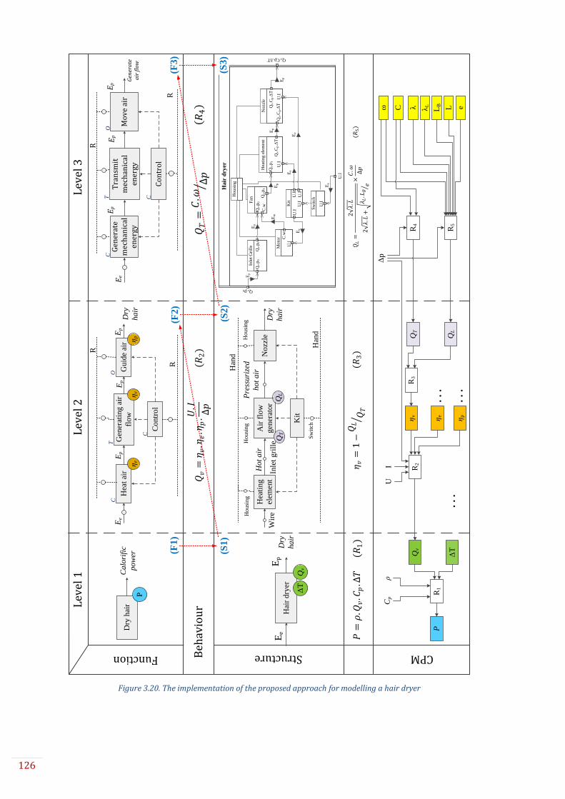
126
Figure 3.20. The implementation of the proposed approach for modelling a hair dryer
P
Qv
ΔT
R1
UI R
2
Δp
ηv
ρ
Cp
ηe
ηp
R3
QT
QL
R4
R5
…… …
ω
C λ
eλL
LB L
Function Structure CPMBeh
avio
ur
Air
flo
w
gen
erat
or
Hea
ting
elem
ent
Nozz
le
Kit
Hot
air
Pre
ssuri
zed
hot
airH
and
Han
d
Dry
hair
Sw
itch
Wir
eHo
usi
ng
Inle
t gri
lleH
ou
sin
gH
ou
sin
g
QT
QL
Gen
erat
ing a
ir
flow
Hea
t ai
rG
uid
e ai
r
Contr
ol
Ee
Ep
Ep
Ep
R
ηe
ηv
R
Dry
hair
ηp
Lev
el 1
Lev
el 2
Lev
el 3
Tra
nsm
it
mec
han
ical
en
ergy
Gen
erat
e m
ech
anic
al
ener
gyM
ov
e ai
r
Co
ntr
ol
Ee
Ep
Ep
Ep
R
R
Gen
era
te
air
flo
w
Ha
ir d
ryer
Kit
U.I
U.I
Ee
Fan
C.w
Qv.p
0
Ee
Inle
t G
rill
eE
p
Qv.p
0Q
v.p
0
Ep
Hea
tin
g e
lem
ent
U.I
Qv.p
1
Ep
No
zzle
U.I
U.I
Ee
Qv.C
p.Δ
TQ
v.C
p.Δ
T
Ep
Ep
Qv.p
1
Qv.C
p.Δ
T
Mo
tor
U.I
C.w
Em
Sw
itch
U.I
Ho
usi
ng
U.I
Ee
U.I
Qv.Cp.ΔT
Qv.p0
CT
O
C
CT
O
C
𝑃=𝜌
.𝑄𝑣
.𝐶𝑝
.∆𝑇
(𝑅1
) 𝜂𝑣
=1−𝑄𝐿𝑄𝑇
⁄
(𝑅
3)
𝑄𝐿
=2√𝜆
.𝐿
2√𝜆
.𝐿+√𝜆𝐿
.𝐿𝐵𝑒⁄
×𝐶
.𝜔 ∆𝑝
(𝑅
5)
Dry
hai
r
P
Calo
rifi
c
pow
er
Hai
r dry
erE
eE
p
ΔT
Qv
Dry
hair
(F1
)
(S1
)
(F2
)
(S2
)
(F3
)
(S3
)
𝑄𝑣
=𝜂𝑣
.𝜂𝑒
.𝜂𝑝
.𝑈.𝐼
∆𝑝
(𝑅
2)
𝑄𝑇
=𝐶
.𝜔∆𝑝
⁄
(𝑅
4)

127

128
CHAPTER 4
1) LR: Concurrent design
2) LR: Complexity
3) LR: DTMs
4) Choosing the best
5) Creation of the Product design approach
6) Repetition of step 3 and 4.
7) Experimentation: Product design approach
8) Experimentation: Product design approach on another case study
9) Improvement of the product design approach
10) Concurrent design approach
11) Experimentation: Concurrent design approach
12) Modification on the product approach for concurrent design.
13) Sensitivity analysis
14) Uncertainty management
15) Tolerance optimisation
16) Conclusion
6. IPPM
5. Uncertainty & Complexity management
4. Case study
3. Product
2. Literature Review
1. Introduction
1.1. Context
1.2. Research questions
1.3. Research objectives
1.4. Methodology
1.5. Thesis outline
2.1. Context
2.2. Value
2.3. Concurrent designing
2.4. Complexity
2.5. DTM
3.1. Context
3.2. Extended-CPM
3.3. Energy flow modelling
3.4. Product modelling approach
3.5. Mini case study
4.1. Oil pump
4.2. Product model
4.3. Complementary tools
5.1. Uncertainty management
5.2. Sensitivity analysis
5.3. Tolerance analysis
6.1. Context
6.2. Flows
6.3. CPM in IPPD
6.4. IPPM approach
6.5. Case study
6.6. Tolerance optimisation
Research questions
1. How concurrent designing can profit industry and how to assess value in this concept?
2. What are the sources of complexity in IPPD and how to manage them?
3. How to manage design uncertainty?
4. How to model an integrated product/process system systematically to increase �value ?
5. How the model can be used to analyse and optimise the system?
M e t h o d o l o g y
Conclusion

129
CHAPTER 4:
Case Study: Product Modelling Approach
This chapter is a detailed case study to demonstrate how the approach is applied. This chapter
focuses on product design aspect of the approach. The objective is to model a system to be used for
designing a product in order to deliver oil in a car engine for lubrication of the parts. One of the
possible solutions is an external gear oil pump that is used in this chapter as a case study. First a
short introduction of the oil pump is presented. Then, by using the proposed approach the system is
modelled. Although the solution for the objective is known, the implementation of the approach will
be explained as it is shown in chapter 3 to emphasise the transition from functional requirements
to the physical structure. After that, several complementary tools that can be used in the approach
are presented. The necessity of these tools is related to the case and the objective is to help to
extract enough information for determining each model in the approach.

130
4.1. Oil pump: a state of the art
Pumps are devices used to generate flow and transmit fluids. There are different types of
pump characterized by its displacement, level of supported pressure, efficiency etc. Generally
pumps are divided into centrifugal and positive displacement pumps. Positive displacement
pumps which include rotary, reciprocating and linear-type pumps make a fluid move by
trapping a fixed amount and forcing it into the discharge pipe. Common types of pumps are
shown in Figure 4.1.
Figure 4.1. Classifications of common pumps
Among different types of pumps, external gear pump is chosen as the case study in this
chapter. This pump uses two gears which rotate inversely to deliver the oil. External gear pumps
have close tolerances and shaft support on both sides of the gears. This allows them to run to
pressures beyond 3,000 PSI / 200 bar, making them well suited for use in hydraulics. Usually in
car engines it has the pressure up to 20 bar. Additionally, due to the low cost of these types of oil
pumps compared to similar models, it is used for car engines. Usually in car engines it has the
pressure up to 20 bar. A simple schema of an external gear pump mechanism is demonstrated in
Figure 4.2.
Figure 4.2. Mechanism of an external gear pump
Advantages and disadvantages of this kind of pump in addition to its application in
industry is summarised in Table 4.1.
Rotary
Gear
External gear
Internal gear
Gear ring
Lobe
Screw Suttle block Vane
Single Chamber
Double Chamber
Reciprocating
Diaphragm Piston
Axial piston
Radial piston
Linear
Rope Chain
Hydraulic pumps

131
Table 4.1. Pros, cons and application of an external gear oil pump
Advantages Disadvantages Applications
High speed
High pressure
No overhung bearing loads
Relatively quiet operation
Design accommodates wide variety of materials
Four bushings in liquid area
No solids allowed
Fixed End Clearances
Various fuel oils and lube oils
Chemical additive and polymer metering
Chemical mixing and blending (double pump)
Industrial and mobile hydraulic applications (log splitters, lifts, etc.)
Acids and caustic (stainless steel or composite construction)
Low volume transfer or application
The type of external gear oil pump is used in this chapter is the one that is used in Renault
Laguna car. An image of this pump is shown in Figure 4.3. In this pump, by using the received
mechanical energy from the engine, it creates hydraulic energy. The hydraulic energy pulls the
oil from the tank and injects it to the engine parts for lubrication. Lubrication in engine is crucial
to reduce the heat and friction of the parts.
Figure 4.3. Laguna oil pump
For better study of this pump, a 3D model of it is illustrated in Figure 4.4. The pump casing
consists of two main parts of CRPH and CPHF. Inside the CPHF, there are two small pinions, a big
shaft to transmit the energy from the sprocket and finally there are fixation screws to assemble
two parts of the casing after the pinions have been inserted. The position of the pump in the
engine casing is as shown in the left side of Figure 4.4. The ending of CRPH, which includes a
seam and grill, is placed in an oil pan (sump) which is part of the engine casing. From the created
hydraulic energy, the oil is sucked up and after passing through the pinions, it exists from the
other side of the pump.
Figure 4.4. 3D model of an oil pump used in Renault Laguna

132
4.2. Product modelling
In this section, the employment of the proposed approach on this case study is presented.
It will be shown how modelling such system with limited knowledge about the structure of the
system is possible.
The proposed approach of chapter 3 can be used in two ways. First, when the product
does not exist and the approach is used for designing a new product. In this case, the proposed
approach determines the system’s models based on the required function. Thanks to the
function-structure link in the approach, the designer can use the model to increase their
knowledge about the designing system. The second way is when the product exists and the
objective is to model the product to optimize the performance of the product. In both ways, the
information about the modelling system should be gathered. In the second case, it is of course
easier to have this information. The complementary tools are presented in 4.3.
In this chapter, considering the studying case, the knowledge of the designer about the
system is quite good because it is about analysing an existing product. If not, the functional
aspect of the approach should be emphasised. So, the decisions toward obtaining a structural
solution are already taken. But the approach will be explained step by step as if the product does
not exist. Although, for modelling a non-existing product, this is the only possible way of using
the proposed approach, it is recommended to use the same technique for an existing product
too. Firstly because the decisions in each level of the approach are made clearly and
systematically. So, the changes (toward optimisation) that might be in any level of
decomposition can be done in the same level. Secondly, because then it will be extended for
concurrent designing by integrating cost analysis (as presented in chapter 6). So, the decisions in
each level of decomposition will be made according to cost considerations also.
The objective in this case study is to deliver the oil with specific flow to the engine parts
for lubrication. As one of the possible solutions for satisfying this function, a car gear pump is
used to analyse. So, the objective is not to model an oil pump but to determine a model that
satisfies the function.
4.2.1. Level 1- System analysis
The study begins with identifying/defining the main function of the system to satisfy the
required output. The main function is to “deliver oil” and the required output is “required flow”
(RQ). So, the first model of the system as a black box will be as Figure 4.5(a). This model
illustrates the objective of the modelling.
In an energy flow approach, the input, the output and the function need to be defined
accordingly. Regarding the required output of the system, hydraulic energy is the output. The
input depends on the chosen/considered solution. As also demonstrated in the primary flow
analysis, in this case, the input energy can be taken from the engine. So, the input is mechanical
energy. Therefore, the function of the system can be defined as the conversion of mechanical
energy into hydraulic energy.
The structural model in each level of decomposition is created based on the functional
model of that level. So, based on the model in Figure 4.5(a), the structural model is created as
Figure 4.5(b). In this model, the product is used for satisfying the required output. The required
output is imposed by the manufacturer to have a flow of at least 5.46×10⁻⁴ m3/s in minimum
RPM for a car in idle state to have enough flow for lubrication of parts. According to this

133
required output, RPj is the required flow (RQ) and based on that the as-is-property is defined as
Q (oil flow). So, the first level of the approach is illustrated as Figure 4.5.
Figure 4.5. First level of modelling approach for an oil pump:
(a) functional model (b) structural model (c) product model
4.2.2. Level 2- System decomposition
The second level is the decomposition of the system into sub-systems. At any level, first
the functional study is done and then it is the structural study accordingly. The system function
is divided into subsystems based on the elements of CTOC. The main sub-function is “to generate
hydraulic energy” so it is the element of Operator. The input for this sub-system is mechanical
energy. However, an element of Transmitter is needed to transmit the received energy from the
engine into the zone of operation. In addition, the element of Control is needed to assure the
pressure of outlet oil flow. In this system, an element of Converter is not needed since the
received type of energy is the desired type (rotational mechanical energy). This functional model
is illustrated in Figure 4.6(a).
One of the important parameters that can be used in this level of functional model is the
efficiency of each sub-system. Since the Transmitter transfers mechanical energy and the
Operator creates hydraulic energy. The hydro-mechanical efficiency (ηhm) and the volumetric
efficiency (ηv) are proper indexes to compare the outlet flow with the inlet flow of the oil and
therefore to be used as IPj. These parameters (ηv, ηhm) are placed in the model as shown in Figure
4.6(b).
In each level of decomposition, the determined parameters create the elements of CPM
step by step. Additionally, the relation (Rm) among the elements should be identified. In order to
obtain this equation, the physical phenomena in the oil pump and its environment have to be
studied. The input is mechanical energy which is received from the engine. So, it includes two
parameters of M (torque) and ω (Angular rotational velocity). These two parameters are related
to the engine behaviour. Therefore, the value of these parameters depends to the condition of
the car which is controlled by the driver. The designer cannot control these parameters while
designing the pump. So, M and ω are two of the ECk.
Fu
nct
ion
Stru
ctu
reC
PM
Level 1
QRQ
(a)
(b)
(c)
To deliver oil
RQ
Required oil
flow to
lubricate parts
Oil pumpEm Eh Required
flow
Q

134
Figure 4.6. Second level of oil pump model: (a) functional model (b) CPM
In addition, the pressure rise (Δp) is a function of Q and it is imposed by the car circuit. As
Figure 4.7 shows part of the energy circuit in the car engine, the mechanical energy (M and ω) is
received by a chain and the pump creates flow with pressure for lubrication in order to reduce
friction and heat in the engine. When the oil circulates in the engine parts, the pressure descends
and then again it is increased by the pump when the flow is generated. So, Δp is not related to
the structure of the pump but to the engine characteristics. Δp cannot be controlled by the
designer in the pump design and it is also considered as an ECk.
Figure 4.7. A simple schema of the energy circuit to illustrate why M, ω and Δp are ECk
Another parameter that has to be considered is temperature. The dilatation impact of
temperature on DC, DG, LC and LG can be calculated as followed:
𝐷𝐶(𝑇) = 𝐷𝐶(𝑇0) × (1 + 𝜏1(𝑇 − 𝑇0)) 𝜏1 = 23.1 × 10⁻⁶𝐾−1 (4.1)
𝐷𝐺(𝑇) = 𝐷𝐺(𝑇0) × (1 + 𝜏2(𝑇 − 𝑇0)) 𝜏2 = 11~13 × 10−6𝐾−1 (4.2)
𝐿𝑐(𝑇) = 𝐿𝑐(𝑇0) × (1 + 𝜏1(𝑇 − 𝑇0)) 𝜏1 = 23.1 × 10⁻⁶𝐾−1 (4.3)
𝐿𝐺(𝑇) = 𝐿𝐺(𝑇0) × (1 + 𝜏2(𝑇 − 𝑇0)) 𝜏2 = 11~13 × 10−6𝐾−1 (4.4)
These parameters are the characteristics of the pinions and casing. The list of all
parameters is available in Appendix A. This aspect is not presented in this case study. However,
Transmit
mechanical
energy
Ø
Generate
hydraulic
energy
Control
Ee Em Em
Eh
R
ηv
Generate
oil flow
ηhm
C T O
C
ηv
ηhm
R1
ω Δp
Q
M
RQ
(a)
(b)

135
later in the calculation, the oil viscosity (μ) is taken into account as an effective parameter. The
effect of temperature is simplified by keeping its value constant. Thus, regarding the parameters
of M, ω, Δp and the efficiencies, R1 is obtained as the first equation for identifying the effective
parameters of Q.
𝑄 =
𝑀.𝜔
∆𝑝× 𝜂𝑣 . 𝜂ℎ𝑚 (𝑅1) (4.5)
According to the functional model in Figure 4.6(a), the necessary decisions are made and
the structural model is created. This model is illustrated in Figure 4.8(a). In Operator element,
the conversion of energy is by means of two gears and a casing. The element of Transmitter
consists of a sprocket, a shaft and two small pinions. These elements must be correctly in
interaction with each other in a proper surrounding (casing) to transfer the energy. The outlet
flow is guided by means of a hose to the required areas to be lubricated. The hose is an
interaction element in CTOC. Moreover, to insure the pressure of the outlet oil an oil regulator is
used as the element of Control. To be noted, in this figure two pinions are placed in both O and T.
The reason is that the volume of pinions transmits the energy while the surfaces generate
pressure on oil.
Figure 4.8. Second level of oil pump model: (a) structural model (b) CPM
The important parameter in transmitting mechanical energy (T) is friction torque (MF).
Since, other than MF, oil displacement (V) and pressure rise (Δp) are also related to ηhm by
considering theoretical torque (M), the efficiency can be calculated as Eq. 4.6.
𝜂ℎ𝑚 =
𝑉
2𝜋. (𝑀 −𝑀𝐹)∆𝑝 (𝑅2) (4.6)
The operator which is responsible for generating hydraulic energy into mechanical energy
has three main parameters as oil displacement (V), velocity (ω) and flow loss (Ql). The relation of
these parameters with the parameters in the previous level (ηv) should be found:
𝜂𝑣 = 1 −
2𝜋. 𝑄𝑙𝑉.𝜔
(𝑅3) (4.7)
Sprocket+Shaft
+2 pinionsCar engine Ø
2 Pinions +
Casing
Oil regulator
Hydraulic
hoseChain
C T O
Em Em Em Eh
C
Pump casing
Screws
VQlMF
ηv
ηhm
R1
Δp
Q
M
RQ
V
Ql
R3
R2
ω
MF
MC1
(a)
(b)
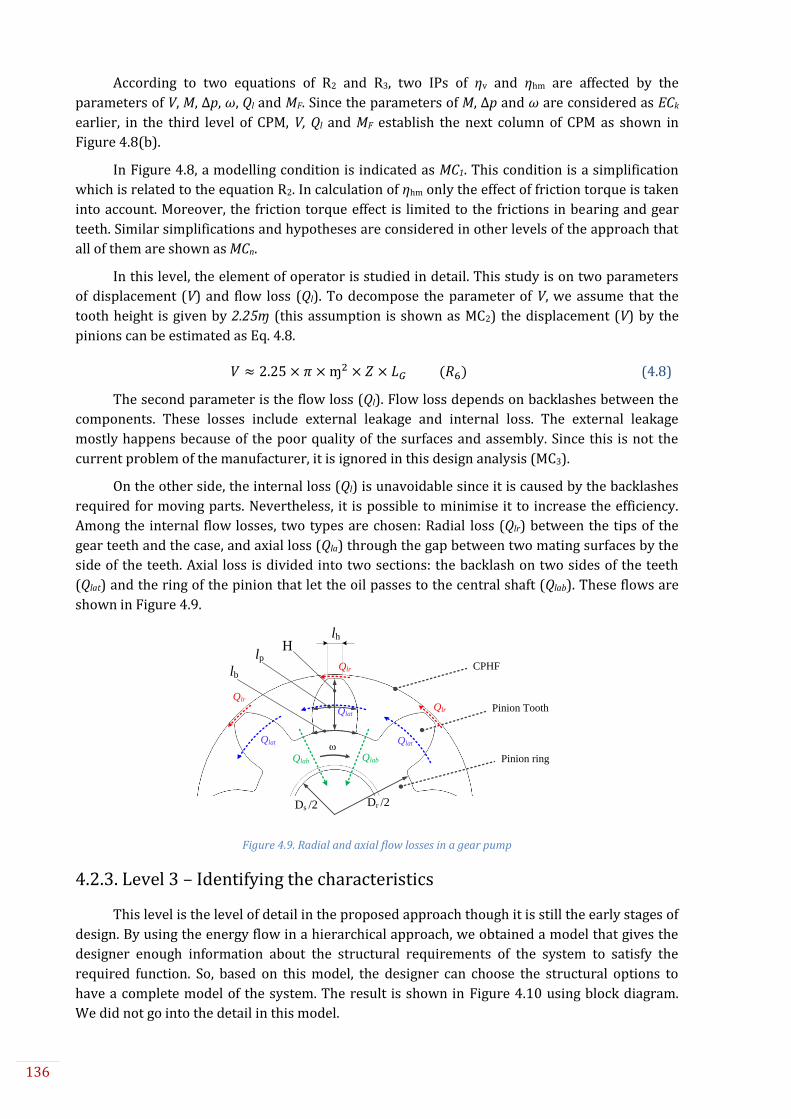
136
According to two equations of R2 and R3, two IPs of ηv and ηhm are affected by the
parameters of V, M, Δp, ω, Ql and MF. Since the parameters of M, Δp and ω are considered as ECk
earlier, in the third level of CPM, V, Ql and MF establish the next column of CPM as shown in
Figure 4.8(b).
In Figure 4.8, a modelling condition is indicated as MC1. This condition is a simplification
which is related to the equation R2. In calculation of ηhm only the effect of friction torque is taken
into account. Moreover, the friction torque effect is limited to the frictions in bearing and gear
teeth. Similar simplifications and hypotheses are considered in other levels of the approach that
all of them are shown as MCn.
In this level, the element of operator is studied in detail. This study is on two parameters
of displacement (V) and flow loss (Ql). To decompose the parameter of V, we assume that the
tooth height is given by 2.25ɱ (this assumption is shown as MC2) the displacement (V) by the
pinions can be estimated as Eq. 4.8.
𝑉 ≈ 2.25 × 𝜋 ×ɱ2 × 𝑍 × 𝐿𝐺 (𝑅6) (4.8)
The second parameter is the flow loss (Ql). Flow loss depends on backlashes between the
components. These losses include external leakage and internal loss. The external leakage
mostly happens because of the poor quality of the surfaces and assembly. Since this is not the
current problem of the manufacturer, it is ignored in this design analysis (MC3).
On the other side, the internal loss (Ql) is unavoidable since it is caused by the backlashes
required for moving parts. Nevertheless, it is possible to minimise it to increase the efficiency.
Among the internal flow losses, two types are chosen: Radial loss (Qlr) between the tips of the
gear teeth and the case, and axial loss (Qla) through the gap between two mating surfaces by the
side of the teeth. Axial loss is divided into two sections: the backlash on two sides of the teeth
(Qlat) and the ring of the pinion that let the oil passes to the central shaft (Qlab). These flows are
shown in Figure 4.9.
Qlat
QlrQlat
Qlat
Qlab Qlab
Qlr
Qlr
ω
CPHF
Pinion Tooth
Pinion ring
Hlp
lb
lh
Dr /2Ds /2
Figure 4.9. Radial and axial flow losses in a gear pump
4.2.3. Level 3 – Identifying the characteristics
This level is the level of detail in the proposed approach though it is still the early stages of
design. By using the energy flow in a hierarchical approach, we obtained a model that gives the
designer enough information about the structural requirements of the system to satisfy the
required function. So, based on this model, the designer can choose the structural options to
have a complete model of the system. The result is shown in Figure 4.10 using block diagram.
We did not go into the detail in this model.

137
Thus, the internal flow loss (Ql) is:
𝑄𝑙 = 𝑄𝑙𝑟 +𝑄𝑙𝑎𝑡 + 𝑄𝑙𝑎𝑏 (𝑅4) (4.9)
Figure 4.10. Level 3: Structural model using block diagram
Two internal properties of V and Ql are decomposed by R6 and R4. The effective
parameters of V in R6 are geometrical dimensions. These parameters, based on the definition,
are Characteristics (Ci). Though, Ql is decomposed into three types of internal flow losses. These
parameters are in the category of IPj yet. So the sub-system needs to be decomposed further and
the effective parameters need to be determined.
To continue the synthesis phase in this level of decomposition, three effective parameters
need to be decomposed. The radial flow loss is because of the backlashes between the teeth of
the gear and the casing. In Figure 4.9 this backlash which is shown as Qlr is calculated as (R7).
This formula is obtained from the Poiseuille equation. It is multiplied by two because of the
existence of two gears in the pump. (Z - 3) denotes the number of teeth where radial flows exist.
𝑄𝑙𝑟 = 2 ×𝐿𝐺ℎ𝑟̅̅ ̅
3
8𝜇 × (𝑍 − 3)𝑙ℎ∆𝑝̅̅̅̅ (𝑅7) (4.10)
The axial backlash which causes the axial flow loss is on the two sides of the gears and the
casing. This flow loss in the area that two gears are engaged acts differently which is shown in
Figure 4.11. Considering the backlash on the two sides of each gear and using Poiseuille
equation, the flow loss is calculated as Eq. 4.11.
𝑄𝑙𝑎𝑡 =𝐻
8𝜇 × √𝑙ℎ . 𝑙𝑝. 𝑙𝑏3
(ℎ𝑎̅̅ ̅2⁄ )
3
. (2
3+
4
𝑍 − 3)∆𝑝̅̅̅̅ (𝑅8) (4.11)
In the formula, √𝑙ℎ . 𝑙𝑝. 𝑙𝑏3 is an estimation of the average tooth width. The third type of
flow loss, due to the axial backlash between the gear and casing and to the direction of the shaft,
is calculated as Eq. 4.12.
ibd
Oil pump
Characteristics:
LC, DC, Dr, Db
CPHF
Eh
Characteristics:
Ds, Ls
Big shaftSprocket
Em
Em
Characteristics:
m, Z, H, lp, lh, lb,
LG, DG, Ds
Pinion 1
Em
Oil regulator
Eh
Eh
Characteristics:Ds, Ls
Small shaftCRPH
Characteristics:m, Z, H, lp, lh, lb, LG, DG, Ds
Pinion 2
Em
Eh
Eh Eh

138
𝑄𝑙𝑎𝑏 = 4 ×
2𝜋 (ℎ𝑎̅̅ ̅2⁄ )
3
8𝜇. ln (𝐷𝑟𝐷𝑠⁄ )
∆𝑝 (𝑅9) (4.12)
For better understanding of the obtained formulas, Figure 4.11 illustrates the backlashes
accompanied by the related geometrical dimensions. The list of these parameters in addition to
all other parameters in this case study is gathered in the table in the Appendix A.
Figure 4.11. Backlashes in an external gear pump
It is important to remind that the objective of this study is not to model the exact flow of
the oil pump as it is similarly done by (Casoli, Vacca, & Berta, 2008; Liping, Yan, Fanli, Jianjun, &
Xianzhao, 2011; Mucchi, Dalpiaz, & Fernàndez Del Rincòn, 2015; Mucchi, Rivola, & Dalpiaz, 2014;
Osiński, Deptuła, & Partyka, 2013), but to have a close-to-reality functioning model to only show
the proposed approach. So, the equations are simplified and other losses are ignored (MC4). In
addition, it is assumed that, gears are perfectly cantered in the casing (MC5). But in reality, the
axial backlash changes all the time during the rotation and calculation of the flow and pressure
distributions are more complicated than the way presented here since they are pulsatory and
transient (Casoli, Vacca, & Franzoni, 2005; Vacca, Franzoni, & Casoli, 2007)
In R7, R8 and R9 all the parameters are Ci except the backlashes (ha and hr). So, as before,
the related formulas need to be determined. Every backlash is related to at least two geometrical
dimensions (Eq. 4.13 and Eq. 4.14)
ℎ𝑟̅̅ ̅ =
𝑀𝑖𝑛(𝐷𝑐) − 𝑀𝑎𝑥(𝐷𝐺 + 𝐴𝑥)
2 (𝑅12) (4.13)
ℎ𝑎̅̅ ̅ = 𝑀𝑖𝑛(𝐿𝐶) − 𝑀𝑎𝑥(𝐿𝐺) (𝑅13) (4.14)
Additionally, friction torque (MF) should be decomposed. Considering the gears as moving
parts, in three zones the main friction happens: friction caused by interaction of two
components or meshing zone, friction in bearing and friction between the gears and oil. We
focused on the second and third types. So the friction torque (MF) is divided into MF1 and MF2. So:
LG
LC
DC
AX
DG
/2hr
ha/2
Big shaft
CPHF
Small shaft

139
𝑀𝐹 = 𝑀𝐹1 +𝑀𝐹2 (𝑅5) (4.15)
The bearing friction torque is calculated as R11.
𝑀𝐹1 = (𝜇. 𝐷𝑠. 𝜔.𝐿𝑠2) × (ℎ𝑏 (
4𝜋(1 + 2𝑛2)
(3 − 𝑛2)√𝑛2)) × (
𝐷𝑠2)2
(𝑅11) (4.16)
Where;
𝑛 = √𝐾
√1+𝐾 , and 𝐾 =
−(1−3𝐵2)+((1−3𝐵2)2+8𝐵2)
0.5
2, and 𝐵 =
𝐹
12𝜋.𝜇.𝜔.𝐷𝑠2.𝐿𝑠× (
2ℎ𝑏
𝐷𝑠)2
And the friction torque between the gear teeth and oil is calculated as Eq. 4.17.
𝑀𝐹2 = 𝜇. (
𝐷𝐺2)2
.𝜔. 𝐿𝐺ℎ𝑟
. (4𝜋(1 + 2𝑛𝐺
2)
(𝑛𝐺2 + 2). √1 − 𝑛𝐺
2) × 10−6 ×
𝐷𝐺2 (𝑅10) (4.17)
MF2 depends on hr which is already calculated in R12. MF1 is related to the backlash between
the shaft and bearing (hb). So, it should be calculated as well.
ℎ𝑏 =
𝐷𝑏 − 𝐷𝑠2
(𝑅14) (4.18)
Now that all the required Characteristics (Ci) and external conditions (ECk) are identified,
the CPM representation of the model is complete. This model is shown in CPM section of Figure
4.12. In this figure, all the Ci are located in the rightmost column. So, with the first view of this
model, one can see all the effective modifiable parameters of the system. By the created model
and identified the relations among the parameters, the following equation is obtained:
𝑃𝑗 = 𝑓(𝐶𝑖, 𝐸𝐶𝑘|𝑀𝐶𝑛) ⇒𝑄
= 𝑓(𝑚, 𝑍, 𝑙ℎ , 𝑙𝑝, 𝑙𝑏 , 𝐿𝐺 , 𝐷𝐶 , 𝐷𝐺 , 𝐿𝐶 , 𝐻, 𝐷𝑟, 𝐷𝑠, 𝐷𝑏, 𝐿𝑠, 𝑀, 𝜔, ∆𝑝, 𝜇 | 𝑀𝐶1,𝑀𝐶2,𝑀𝐶3,𝑀𝐶4,𝑀𝐶5) (4.19)
Thanks to this equation, the effect of each Ci or ECk or the combination of them on Q or any
IPj can be analysed by using local sensitivity analysis (Saltelli, Tarantola, Campolongo, & Ratto,
2004). In addition, in a global sensitivity analysis (Saltelli et al., 2008), the importance of each
parameter can be evaluated. This analysis can be used to optimize an existed product or to
design a new product with high efficiency. Sensitivity analysis and optimisation by using this
model will be presented in chapter 6.
4.3. Complementary tools
While following the proposed approach, depending on the case, the designer can use some
complementary tools. The goal is to extract enough information in each level of the approach in
order to determine each model (F1, F2, … S1, S2, …) in the approach. For instance in section 4.3.1
and 4.3.2 few of these tools are presented.
4.3.1. Functional analysis
Functional analysis is done to identify the objective of the system. The objective is to
satisfy the customer need(s). In technical point of view, the customer satisfaction can be
interpreted as the fulfilment of the required function. Of course, customer’s need is not limited

140
to functional requirements. In this report, customer’s need is a product with high value. Value, as
defined in chapter 1, includes two axes of quality and cost. The cost aspect will be discussed in
chapter 6 where both product and process are modelled. The quality aspect, which is the
objective in this chapter, is limited to the functionality of the product.
Figure 4.12. A global illustration of the proposed approach for modelling an oil pump
Functional analysis is a tool to evaluate the customer satisfaction which in our case means
product functionality. By means of this tool, we identify the functions of the product to evaluate.
In addition, it shows the relations among the components of the product as well as between the
product and other components of the system in terms of functionality. In a deeper level of study,
function analysis gives us the liaisons between entities that can be used for structural design.
The first stage is to analyse how the product works and then to characterise the functions.
In this part, the designer needs to answer the questions such as: “what is the purpose of the
function?”, “What is the reason of the function?”, “What are the possible improvements?”, and
“What are the required parameters for this function?”. After analysing all the functions of the
product, we need to examine the significance of each function in the total performance of the
product. The total performance of the product is related to the integrated performance of the
components. Thus, the significance of the function is defined as the relationship of one function
with another.
In functional analysis, as a primary stage, the functions of each component and its
relationships with the main function are studied. The function of the oil pump is divided into
sub-functions of principal functions, control functions and constraint functions. These functions
are defined in Table 4.2.
Fu
nct
ion
Stru
ctu
reC
PM
Transmit
mechanical
energy
Generate
hydraulic
energy
Control
Em EmEh
R
ηv
Generate
oil flowηhm
Deliver oil
Oil pumpEm
Eh
RQ
Level 1 Level 2 Level 3
T O
C
Sprocket+Shaft
+2 pinions
Car
engine
2 Pinions +
Casing
Oil
regulator
Hydraulic
hose
Chain
T OEm Em Eh
C
Generate
oil flow
Pump casing
Screws
ibd
Oil pump
Characteristics:
LC, DC, Dr, Db
CPHF
Eh
Characteristics:
Ds, Ls
Big shaftSprocket
Em
Em
Characteristics:
m, Z, H, lp, lh, lb,
LG, DG, Ds
Pinion 1
Em
Oil regulatorEh
Eh
Characteristics:
Ds, Ls
Small shaft
CRPH
Characteristics:
m, Z, H, lp, lh, lb,
LG, DG, Ds
Pinion 2
Em
Eh Eh
VQlMF
Required
oil flow to
lubricate
parts
Required
flowQ
LG
Zm
ha
V
Ql
ηv
ηhm
R13R3
R2
R4
R6
R1
H
hr
Dr
DC
DG
LC
R12
Ds
lh
Qlr
Qlat
Qlab
R7
R8
R9
ω M
Q
lp
lb
MC1 MC2
MC3MC4
MC4
MC4
MC5
MF
Db
Ls
MF1
MF2R5
R11
R10
hb R14
µ, ω, Δp
µ, ω, Δp
RQ
µ ∆p
Eh

141
Table 4.2. Sub-functions of a car oil pump
Pump in work: Pump in idle time or maintenance:
Principal functions:
PF1: Transform the mechanical energy into hydraulic energy.
PF2: Deliver the oil to the engine
Control Functions:
CO1: Accumulate and regulate oil pressure.
CO2: Prevent all the oil leaks to the surroundings environment
CO3: Prevent the oil leakage in idle state
CO4: Easy assembly and disassembly
Constraint:
CF1: Adapt the pump on different engine casings.
CF2: Motorise the pump and respect the rotation limits.
CF3: Not to trouble the user of the car (sound and vision)
CF4: Resist to the external environment
CF5: Have a link to the engine casing in working and idle state
CF6: Keep the oil waiting for utilization in idle state
CF7: Accessibility to the pump in the engine casing
CF8: Respect the environment
In order to illustrate the function of the product and its relationship with other
components, “Diagramme Pieuvre” (In French) is used. This diagram is used to analyse the needs
and to identify the functions of a product. Figure 4.13 is the diagramme pieuvre of the pump in
work, idle time and during the maintenance.
Oil PumpCF7
CO1
CO2
PF1
PF2
CO3
CO4
Engine casing Oil
User Crankshaft
Outward Environement
CF8
Figure 4.13. ‘Diagramme Pieuvre’ of the oil pump
As Figure 4.13 demonstrates, the main functions relate the pump to the crankshaft (to take
the energy) and engine casing (including the parts to lubricate). The oil circulates from the sump
which is part of the engine casing to the engine components and back to the sump. There are
also interactions with human including the driver and the repairman. Moreover, the impact of
the external environment should be considered. This diagram can be used as a primary tool to
be used for starting the proposed approach of chapter 3. Whether the product exists or not, this
analysis can be done to identify the interaction of the designing system with the environment.
If we consider the analysis of Figure 4.13 as the product level, the next level of analysis
would be entities or features. For feature analysis level, the component CPHF is chosen. Figure
4.14 illustrates this component with highlighting its important features.

142
For identifying the relationships of the features with the functions, TAFT2 is used. This tool
which is proposed by Charpentier & Mathieu (2000) capitalises all the required information for
functional specification of the components. Geometrical functional requirement analysis of the
product is the key step for improving the product design (Charpentier & Mathieu, 2000). This
table analyses every entity of the system regarding the related action toward satisfying the
required function of the system. Table 4.3 shows the first two parts of this table for the
component CPHF.
Figure 4.14. Draft of the oil pump’s component (CPHF) and its important features
The first section of this table is the description of the technical functions. In this section,
the different actions of the part are marked with the related component. Action means how the
entity is related to the function. The second column of the table is the related geometrical
elements. Meaning, the surfaces related to each action and the studying component (CPHF). The
third column shows the type of link. In the second section, the related entities (surfaces) are
pointed out regarding Figure 4.14. There can be several contact surfaces for one action, and a
single surface can also satisfy several actions.
Table 4.3. Section 1 and 2 of TAFT for CPHF
No. Identification-Action Liaisons - Surfaces
ETF3 on
what Complement Complementary remarks Surf.1 Surf.2 Surf. 3
1 Positioning CRPH Axially The action characterizes the quality of correct positioning of CPHC on CRPH
PL100 FI10x
2 Prevent
the leakage CRPH Flux
The action characterizes the static sealing of the connection
PL100 FI10x
3 Positioning CRPH With pressure The action characterizes the static sealing of the connection
PL100 FI10x
4 Positioning 4 x
Screw Axially
The action characterizes the precision of the axial position of the 4 screws on CPHC
FI10x
5 Positioning 4 x
Screw Angularly
The action characterizes the precision of the angular position of the 4 screws separately on CPHC
FI10x
6 Passing 4 x
Screw Radially
The action characterizes the passage of the screws in the part without barrier
FI10x
7 Positioning Engine casing
Axially The action characterizes the precision of positioning on the engine casing during
PL101 CY109 CY108
2 TAFT : Technical function analysis table (Tableau Analyse Fonctionnelle Technique)
3 Elementary Technical Function
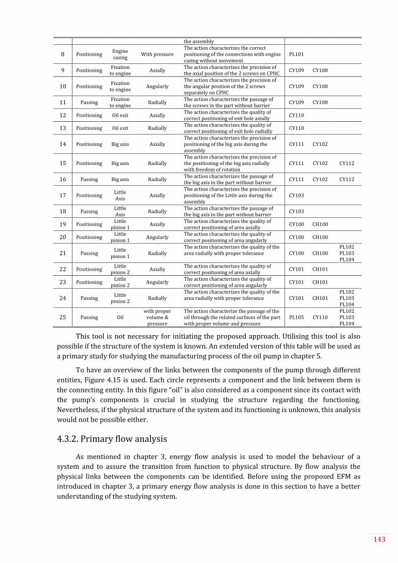
143
the assembly
8 Positioning Engine casing
With pressure The action characterizes the correct positioning of the connections with engine casing without movement
PL101
9 Positioning Fixation
to engine Axially
The action characterizes the precision of the axial position of the 2 screws on CPHC
CY109 CY108
10 Positioning Fixation
to engine Angularly
The action characterizes the precision of the angular position of the 2 screws separately on CPHC
CY109 CY108
11 Passing Fixation
to engine Radially
The action characterizes the passage of the screws in the part without barrier
CY109 CY108
12 Positioning Oil exit Axially The action characterizes the quality of correct positioning of exit hole axially
CY110
13 Positioning Oil exit Radially The action characterizes the quality of correct positioning of exit hole radially
CY110
14 Positioning Big axis Axially The action characterizes the precision of positioning of the big axis during the assembly
CY111 CY102
15 Positioning Big axis Radially The action characterizes the precision of the positioning of the big axis radially with freedom of rotation
CY111 CY102 CY112
16 Passing Big axis Radially The action characterizes the passage of the big axis in the part without barrier
CY111 CY102 CY112
17 Positioning Little Axis
Axially The action characterizes the precision of positioning of the Little axis during the assembly
CY103
18 Passing Little Axis
Radially The action characterizes the passage of the big axis in the part without barrier
CY103
19 Positioning Little
pinion 1 Axially
The action characterizes the quality of correct positioning of area axially
CY100 CH100
20 Positioning Little
pinion 1 Angularly
The action characterizes the quality of correct positioning of area angularly
CY100 CH100
21 Passing Little
pinion 1 Radially
The action characterizes the quality of the area radially with proper tolerance CY100 CH100
PL102 PL103 PL104
22 Positioning Little
pinion 2 Axially
The action characterizes the quality of correct positioning of area axially
CY101 CH101
23 Positioning Little
pinion 2 Angularly
The action characterizes the quality of correct positioning of area angularly
CY101 CH101
24 Passing Little
pinion 2 Radially
The action characterizes the quality of the area radially with proper tolerance CY101 CH101
PL102 PL103 PL104
25 Passing Oil with proper
volume & pressure
The action characterize the passage of the oil through the related surfaces of the part with proper volume and pressure
PL105 CY110 PL102 PL103 PL104
This tool is not necessary for initiating the proposed approach. Utilising this tool is also
possible if the structure of the system is known. An extended version of this table will be used as
a primary study for studying the manufacturing process of the oil pump in chapter 5.
To have an overview of the links between the components of the pump through different
entities, Figure 4.15 is used. Each circle represents a component and the link between them is
the connecting entity. In this figure “oil” is also considered as a component since its contact with
the pump’s components is crucial in studying the structure regarding the functioning.
Nevertheless, if the physical structure of the system and its functioning is unknown, this analysis
would not be possible either.
4.3.2. Primary flow analysis
As mentioned in chapter 3, energy flow analysis is used to model the behaviour of a
system and to assure the transition from function to physical structure. By flow analysis the
physical links between the components can be identified. Before using the proposed EFM as
introduced in chapter 3, a primary energy flow analysis is done in this section to have a better
understanding of the studying system.

144
Screws
x 4
Screws
x 4
CRPHCRPH
Engine
casing
Engine
casing
CPHFCPHF
Dent
CY
Dent
CY
Pinion 2Pinion 2 Dent
CY
CY103
PL100
With pressure
FI10x
Fixation
to engine
Fixation
to engineCY108
PL101
With pressure CY110
CY
CY100
Dent with liquid
Dent with liquid
CY
PL
CY//
Seam
Big
Shaft
Big
Shaft
SprocketSprocket
ChainChain
Pinion 1Pinion 1
Small
shaft
Small
shaft
FlexibleFlexible
OILOIL
Oil filterOil filterCrankshaftCrankshaft CamshaftCamshaft
External
Environ
ment
External
Environ
ment
CY101
PL104
PL103
CY110
PL102
CY109
Flexible
connection
Flexible
connection
CY
CY102
CY111
Figure 4.15. Components’ interaction analysis through the entities
Like in functional analysis, here, the energy flow is studied in levels of product,
components and features. As Figure 4.16 shows, the mechanical energy is received by the
engine. By created hydraulic energy in the pump, the oil is pulled from the sump (Engine low
part) and after passing through the filter and tubes, it goes to engine parts for lubrication. After
that, it returns to the sump.
Engine
top part
Filter &
flexibleOil pump
Engine
low part
E. hyd.
E. hyd.
E. hyd.
E. hyd.
E. mech.
Figure 4.16. Energy flow in oil pump (product level)
In order to show the important energy flows, the diagram in Figure 4.15 is used. The
important energy flows in an oil pump are mechanical energy, hydraulic energy and thermal
energy. Figure 4.17 illustrates these flows through the component using the related entities.
These diagrams can be used to identify the energy circuit in the system. For this analysis Block
Diagram can be used too.
These tools are used to create the link between function and structure of a system. The
drawback of these tools is that mostly are based on the physical structure of the system. When
designing a new system, the required information for using these tools is not available.
Moreover, their links are not mathematical.

145
4.4. Conclusion
This chapter has described a complete deployment of the proposed approach (presented
in chapter 3) on an industrial case study to demonstrate how the approach helps the designer in
transition from function to structure.
The approach aims at identifying the minimum physical requirements of a system in order
to satisfy the required function. The required function has defined as “to deliver oil”. In energy
point of view and regarding the target application of the product (lubrication of engine parts),
the function has been interpreted as the conversion of mechanical energy into hydraulic energy.
The approach includes three sections: functional domain, structural domain and model section
using CPM. By zigzagging between these two domains, the system is studied in a top-down
approach and the model is determined as it is decomposed in each level. The rightmost column
in CPM (characteristics) illustrates the effective modifiable parameters of the physical structure
of the system on the function. All the relations (Rm) in the model are related and create one
formula which links the functional requirement (RQ) to the minimum physical structure (Ci).
The completeness of the model is related to the objective of the designer. In other words, it
depends what the designer is looking for by modelling the system. When the objective is the
optimisation of the performance by modifying a specific part of a product, the decomposition
will be in that specific direction.
In this case, identifying the geometrical characteristics of one component (CPHF) that are
effective on the pump performance was the objective of the designer. Depends on the level of
decomposition and the physical relationships (functional or/and structural) other components
are taken into account to some extend even in the most decomposed level (e.g. dimensions of the
pinions). Moreover, only two phenomena of internal flow loss and friction have been studied.
These help the designer to focus on the aspect of the system that matters.
Determining the model in an unknown system is directly related to the designer’s
expertise regarding the related phenomena and identifying the correct formulas. This issue can
be considered as a weakness of the approach. However, studying the system in two axes of
decomposition and mapping systematically as proposed can help the designer to know where to
look for. For instance, when oil flow (Q) is required as an output, flow loss is calculated (Ql).
Then, the phenomena that are related to flow loss are studied. Finally, how tolerancing and
geometrical dimensions can effect on those phenomena. In another example, the effect of friction
on the performance has been studied. So, the approach creates these links.
In the next chapter it is shown how this approach can be used for uncertainty
management and complexity management. The next chapter will also focus on phase 2 of the
approach to analyse the system based on the determined model to identify the key
characteristics. Chapter 6 is an extension of this approach that can be used to model
manufacturing system in an integrated product and process design environment. The same case
study that is studied in this chapter will be used. The difference is that, in each level of
decomposition, the decisions are made by involving the factor of cost too.

146
Screws
x 4
Screws
x 4
CRPHCRPH
Engine
casing
Engine
casing
CPHFCPHF
Dent
CY
Dent
CY
Pinion 2Pinion 2Dent
CY
CY103
PL100
With pressure
FI10x
Fixation
to engine
Fixation
to engineCY108
PL101
With pressure CY110
CY
CY100
Dent with liquid
Dent with liquid
CY
PL
CY//
Seam
Big
Shaft
Big
Shaft
SprocketSprocket
ChainChain
Pinion 1Pinion 1
Small
shaft
Small
shaft
FlexibleFlexible
OILOIL
Oil filterOil filterCrankshaftCrankshaft CamshaftCamshaft
External
Environ
ment
External
Environ
ment
CY101
PL104
PL103
CY110
PL102
CY109
Flexible
connection
Flexible
connection
CY
CY102
CY111
(a)
Screws
x 4
Screws
x 4
CRPHCRPH
Engine
casing
Engine
casing
CPHFCPHF
Dent
CY
Dent
CY
Pinion 2Pinion 2 Dent
CY
CY103
PL100
With pressure
FI10x
Fixation
to engine
Fixation
to engineCY108
PL101
With pressure CY110
CY
CY100
Dent with liquid
Dent with liquid
CY
PL
CY//
Seam
Big
Shaft
Big
Shaft
SprocketSprocket
ChainChain
Pinion 1 Pinion 1
Small
shaft
Small
shaft
FlexibleFlexible
OILOIL
Oil filterOil filterCrankshaftCrankshaft CamshaftCamshaft
External
Environ
ment
External
Environ
ment
CY101
PL104
PL103
CY110
PL102
CY109
Flexible
connection
Flexible
connection
CY
CY102
CY111
(b)
Screws
x 4
Screws
x 4
CRPHCRPH
Engine
casing
Engine
casing
CPHFCPHF
Dent
CY
Dent
CY
Pinion 2Pinion 2 Dent
CY
CY103
PL100
With pressure
FI10x
Fixation
to engine
Fixation
to engineCY108
PL101
With pressure CY110
CY
CY100
Dent with liquid
Dent with liquid
CY
PL
CY//
Seam
Big
Shaft
Big
Shaft
SprocketSprocket
ChainChain
Pinion 1Pinion 1
Small
shaft
Small
shaft
FlexibleFlexible
OILOIL
Oil filterOil filterCrankshaftCrankshaft CamshaftCamshaft
External
Environ
ment
External
Environ
ment
CY101
PL104
PL103
CY110
PL102
CY109
Flexible
connection
Flexible
connection
CY
CY102
CY111
(c)
Figure 4.17. The energy flows through the components a) Mechanical energy, b) Hydraulic energy, c) Thermal energy

147
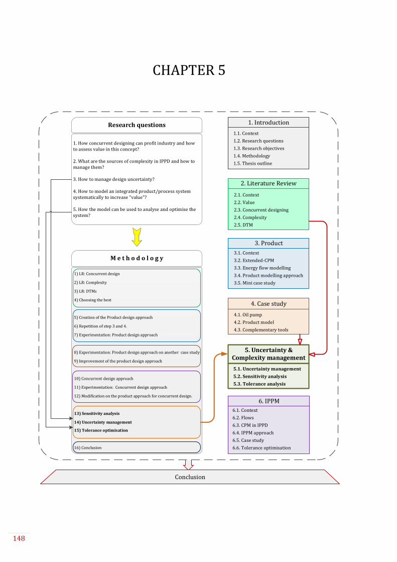
148
CHAPTER 5
1) LR: Concurrent design
2) LR: Complexity
3) LR: DTMs
4) Choosing the best
5) Creation of the Product design approach
6) Repetition of step 3 and 4.
7) Experimentation: Product design approach
8) Experimentation: Product design approach on another case study
9) Improvement of the product design approach
10) Concurrent design approach
11) Experimentation: Concurrent design approach
12) Modification on the product approach for concurrent design.
13) Sensitivity analysis
14) Uncertainty management
15) Tolerance optimisation
16) Conclusion
6. IPPM
5. Uncertainty & Complexity management
4. Case study
3. Product
2. Literature Review
1. Introduction
1.1. Context
1.2. Research questions
1.3. Research objectives
1.4. Methodology
1.5. Thesis outline
2.1. Context
2.2. Value
2.3. Concurrent designing
2.4. Complexity
2.5. DTM
3.1. Context
3.2. Extended-CPM
3.3. Energy flow modelling
3.4. Product modelling approach
3.5. Mini case study
4.1. Oil pump
4.2. Product model
4.3. Complementary tools
5.1. Uncertainty management
5.2. Sensitivity analysis
5.3. Tolerance analysis
6.1. Context
6.2. Flows
6.3. CPM in IPPD
6.4. IPPM approach
6.5. Case study
6.6. Tolerance optimisation
Research questions
1. How concurrent designing can profit industry and how to assess value in this concept?
2. What are the sources of complexity in IPPD and how to manage them?
3. How to manage design uncertainty?
4. How to model an integrated product/process system systematically to increase �value ?
5. How the model can be used to analyse and optimise the system?
M e t h o d o l o g y
Conclusion

149
CHAPTER 5:
Uncertainty and complexity management in
product design
As discussed in chapter 1 and 2, the main problem in IPPD is complexity. In chapter 3 and 4 a modelling approach has been proposed. The proposed approach gives the designer a pathway to transit from function to structure and identify the effective parameters. Since, one of the reasons for complexity is the links between the elements of design, such approach to identify the important parameters and determine the link between them. However, one of the main sources of complexity is uncertainty in every stage of the design such as in these links. So, in the first section of this chapter, it is shown how the proposed systematic approach can help the designer to manage complexity that is due to uncertainty. After a literature review about different types of uncertainty in design, it is described how the approach can be used for uncertainty elicitation and propagation.
The second phase of the approach is to use the determined model from the first phase to analyse the system. So, the second section is sensitivity analysis of the system by using the created model of the product (or/and process). Thanks to the mathematical relationships in the determined model, the impact of the inputs on the output (local sensitivity analysis) as well as the importance of the input parameters on the functioning of the system (global sensitivity analysis) can be analysed.
In the third section, it is shown how this sensitivity analysis and the approach can be utilised for tolerance analysis. In other words, the effect of tolerancing on quality and cost of the product can be measured. In this section, the focus is on tolerancing in product design. Cost considerations, which are mostly related to the process design, will be discussed in the next chapter.

150
5.1. Uncertainty management
The first section of this chapter illustrates how the proposed approach can help the
designer to manage uncertainty in design process. The exploitation of the approach for
uncertainty management includes two aspects. The first aspect is how to use the approach for
uncertainty elicitation in design process which is a principal requirement for uncertainty
management. The second aspect is using the approach for managing epistemic uncertainty and
therefore reducing design complexity that is due to this type of uncertainty.
So, after a brief literature review on uncertainty and robust design, it is shown how the
approach can help the designer to identify the possible uncertainties. Then, it is explained how
the approach can help the designer to reduce design complexity that is due to the epistemic
uncertainty. In section 5.1.5 uncertainty elicitation on the same case study as chapter 4 is
presented.
5.1.1. Uncertainty taxonomy
Uncertainty is ubiquitous in engineering design. As humanity aims for designing more and
more complicated systems, it is not capable of accurately predicting the behaviour and design
parameters of the designed systems. This inability which can be due to various reasons is
discussed as “uncertainty” in design. Lack of knowledge about a system and its environment,
imperfect manufacturing, coupling of system’s element, errors and many other issues cause the
design to be uncertain. The concept of uncertainty is discussed and classified in different
engineering domains such as system engineering (Klir & Folger, 1988), Civil engineering (Ayyub
& Chao, 1998), structural engineering (Melchers, 1999), aerospace (DeLaurentis & Mavris, 2000)
and mechanical engineering (Otto & Antonsson, 1993). The domain in this chapter is uncertainty
in product modelling and design.
There are different types of uncertainty in modelling and design as well as other fields.
Therefore, there are various classifications in literature. In a classical taxonomy, uncertainty is
divided into aleatory and epistemic. Aleatory uncertainty, which is also referred to as irreducible,
objective, stochastic or type-A uncertainty, is the inherent randomness of a phenomenon
(Dantan et al., 2013; Kiureghian & Ditlevsen, 2009). Epistemic uncertainty, which is also stated
as reducible, subjective or Type-B uncertainty, is due to the lack of knowledge of a system. The
lack of knowledge can be in identifying design parameters, their relationships or in the
behaviour of a system in different conditions or about the appropriate value to use for a quantity
that is assumed to have a fixed value in the context of a specific application (Swiler & Giunta,
2007).
Different types of uncertainty exist in all stages of the design process. Considering the four
phases of the design as mentioned in chapter 1, uncertainty should be identified and managed in
each phase:
1) Planning and task clarification: In this phase there is always epistemic uncertainty in the
precision of collected information about the requirements and constraints.
2) Conceptual design: In this phase possible solution to the design problem is determined.
Epistemic uncertainty in designer’s decisions toward identifying a solution is
unavoidable.

151
3) Embodiment design: The concept obtained in the previous phase is concretised and
detailed in this phase. Different types of epistemic uncertainty in the made decisions,
identified effective factors, determined criteria and behaviour of the system exist as it
will be further discussed in this section.
4) Detail design: In this phase the detail design including forms, shapes, surfaces, tolerances
and material are designed based on the design of previous phase. In addition to the
epistemic uncertainty due to the decisions of this phase or previous phases, the existence
of aleatory uncertainty in the value of physical entities and environmental impacts are
unavoidable.
So, there are different types of uncertainty to identify and manage in the process of
modelling and design. Therefore, we need first to classify types of uncertainty in our domain.
The classical taxonomy as presented has been used as the basis of classification in order to
demonstrate how the proposed approach can be used for uncertainty elicitation and reducing
design complexity due to uncertainty. In addition, the categorization of (Thunnissen, 2005) is
taken into account to focus on uncertainty in modelling and design.
As mentioned earlier, classical taxonomy classified uncertainty types into aleatory and
epistemic. Thunnissen (2005) added two more categories to this taxonomy: Ambiguity and
Interaction. Ambiguity is uncertainty in exact transmission of information between two parties.
While communication between different design departments, between customer and company,
and between supplier and company is important and inevitable, sometimes the understanding of
the received information is not exactly the intent of the information giver. Interaction
uncertainty is related to unanticipated interaction of events or/and disciplines (Thunnissen,
Engelbrecht, & Weiss, 2003). With a step further, Thunnissen et al. (2003) classified epistemic
uncertainty into Model, phenomenological and behavioural uncertainty.
Model uncertainty is in the accuracy of the system’s model regarding the actual system. In
other words, it is the difference between the mathematical model and the real behaviour of the
system. Since, the approach is to model the system; model uncertainty is an important type of
epistemic uncertainty here. Model uncertainty can be due to approximation errors,
programming errors or numerical errors.
Phenomenological uncertainty is related to the behaviour of a system in different
conditions. It can be due to unknown impacts of the environment, unimaginable behaviour of the
system in specific condition, or possible behaviour of the system while using specific design
technique. To model a system, it is necessary to predict its behaviour. Therefore, considering
phenomenological uncertainty is essential.
Behavioural uncertainty is related to the uncertain individual or organizational behaviour.
It can be due to the design decisions that are made during design process, customer or stake
holder requirement uncertainty, uncertainty in future action of the user or organization while
interacting with the system, or human errors during development of a system.
The fourth type of epistemic uncertainty is ambiguity which is related to communication
misunderstanding. Lack of knowledge about the exact transmitted information can be also
considered as epistemic uncertainty. Moreover, interaction uncertainty is related to the lack of
knowledge in the relation of design parameters, different engineering disciplines, and different
aspect of design. So, it can be also placed in epistemic uncertainty.
Therefore here, similar to the classical taxonomy, we divide uncertainty into aleatory and
epistemic one. Though, considering the classification and definitions of different types of
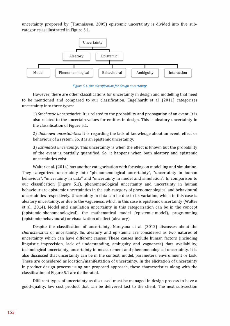
152
uncertainty proposed by (Thunnissen, 2005) epistemic uncertainty is divided into five sub-
categories as illustrated in Figure 5.1.
Figure 5.1. Our classification for design uncertainty
However, there are other classifications for uncertainty in design and modelling that need
to be mentioned and compared to our classification. Engelhardt et al. (2011) categorizes
uncertainty into three types:
1) Stochastic uncertainties: It is related to the probability and propagation of an event. It is
also related to the uncertain values for entities in design. This is aleatory uncertainty in
the classification of Figure 5.1.
2) Unknown uncertainties: It is regarding the lack of knowledge about an event, effect or
behaviour of a system. So, it is an epistemic uncertainty.
3) Estimated uncertainty: This uncertainty is when the effect is known but the probability
of the event is partially quantified. So, it happens when both aleatory and epistemic
uncertainties exist.
Walter et al. (2014) has another categorisation with focusing on modelling and simulation.
They categorized uncertainty into “phenomenological uncertainty”, “uncertainty in human
behaviour”, “uncertainty in data” and “uncertainty in model and simulation”. In comparison to
our classification (Figure 5.1), phenomenological uncertainty and uncertainty in human
behaviour are epistemic uncertainties in the sub-category of phenomenological and behavioural
uncertainties respectively. Uncertainty in data can be due to its variation, which in this case is
aleatory uncertainty, or due to the vagueness, which in this case is epistemic uncertainty (Walter
et al., 2014). Model and simulation uncertainty in this categorization can be in the concept
(epistemic-phenomenological), the mathematical model (epistemic-model), programming
(epistemic-behavioural) or visualization of effect (aleatory).
Despite the classification of uncertainty, Narayana et al. (2012) discusses about the
characteristics of uncertainty. So, aleatory and epistemic are considered as two natures of
uncertainty which can have different causes. These causes include human factors (including
linguistic imprecision, lack of understanding, ambiguity and vagueness) data availability,
technological uncertainty, uncertainty in measurement and phenomenological uncertainty. It is
also discussed that uncertainty can be in the context, model, parameters, environment or task.
These are considered as location/manifestation of uncertainty. In the elicitation of uncertainty
in product design process using our proposed approach, these characteristics along with the
classification of Figure 5.1 are deliberated.
Different types of uncertainty as discussed must be managed in design process to have a
good-quality, low cost product that can be delivered fast to the client. The next sub-section
Uncertainty
Aleatory Epistemic
Model Phenomenological Behavioural Ambiguity Interaction

153
explains the concept of “robust design” which is the most common approach for managing
uncertainty.
5.1.2. Robust design
In order to manage uncertainty, there are two primary approaches. The first approach is
to reduce uncertainty itself. This reduction is feasible when large amount of data is available or
the designer has rather complete knowledge of a system. In designing a new (innovative)
product having this kind of knowledge is not possible. This emphasises the importance of
“robust design” as the second approach.
Robust design, which is first introduced by Taguchi in 1958, is to design a product or
process insensitive to variations. Robust design is to improve the quality of products and
processes by reducing their sensitivity to variations, thereby reducing the effects of variability
without removing its sources (Taguchi 1986, 1990). Suh (2005) defined robust design as “a
design that is able to accommodate large variation in design parameters and process variables and
yet still satisfy the functional requirements”.
In robust design, there are three types of information: Control factors, noise factors and
responses. Control factors or design parameters are the parameters that the designer can adjust.
This is similar to the characteristics (Ci) in CPM ontology. Noise factors are the environmental
impact on a system that the designer cannot control. In CPM, these parameters are called
external conditions (ECk). Finally, responses are the output of a system or as-is properties (Pj) in
CPM. These types of information are shown in Figure 5.2.
System
Noise factors
(ECk)
Control factors
(Ci)
Responses
(Pj)
Figure 5.2. Types of information in robust design and the equivalent in CPM
According to McDowell et al. (2010) there are three possible ways for robust design
identification:
1) Identify control factor (design variable) values that satisfy a set of performance
requirement targets despite variation in noise factors.
2) Identify control factor (design variable) values that satisfy a set of performance
requirement targets despite variation in control and noise factors.
3) Identify adjustable ranges for control factors (design variables), that satisfy a ranged set
of performance requirements and are insensitive to the variability within the model.
Choi (2005) categorises robust design into four types. Type-I robust design is related to
uncertainty in identifying design variable or (control factor) values to satisfy the required
performance in spite of the variations in noise factors (Allen et al., 2006) which is aleatory
uncertainty. Type-II is about uncertainty in control factors which is also aleatory uncertainty.
Type-III is related to the identification of adjustable ranges for control factors to satisfy the
required performance and is insensitive to variations within the model. This type is related to

154
both aleatory and epistemic uncertainty. For example, a model may incorporate simplifying
assumptions or random factors.
Figure 5.3 is Type-III robust design. The same objective function curve is utilised for Type
I and II in comparison with Type-I, -II and -III robust solution. Regarding the objective function
and upper and lower limits, Type-I and Type-II have larger performance deviation than Type-I, -
II and -III. So, for propagation of uncertainty in design process, especially in modern engineering
systems as they are getting more and more complex with stochastic behaviour, Type-III is very
important. In order to do that, managing both epistemic and aleatory uncertainty is necessary.
Figure 5.3. Type-III robust design (Choi, 2005)
Type-IV is related to the model uncertainty including errors in decisions and accumulated
errors by series of uncertain subsystem models (Choi, 2005). This downstream effect of
uncertainty is shown in Figure 5.4. This is the main reason that while focusing on uncertainty in
embodiment and detail design phases, uncertainties in the first two phases of design should be
paid attention too.
Figure 5.4. The downstream uncertainty effect in type-IV robust design (Allen et al., 2006; Choi, 2005)
Equivalent in CPM:
Control Factors: Ci
Interdependent Responses: IPj
Independent Responses: Pj
Noise Factors: ECk
(Pj)
(Ci)

155
Considering all these types of robust design, the objective in robust design is to achieve an
optimal result with minimum variability. However, there are difficulties in implementation of
the optimisation methods in robust design. As (R. Roy, Hinduja, & Teti, 2008) stated,
optimization problems in design can be because of the number of design variables, their nature
(static or dynamic), admissible values (integer, continuous, or mixed) or because of the number
of constraints and number of objective functions.
In some of the decision making methods in design, companies use the method of
eliminating less optimized solutions in each level and by this way they reduce the number of
calculations. However, even weak solutions can be criterion with some small changes. Thus,
design decision making is not a strict mathematical way. Therefore, to find the optimal solution,
we must rank not only desirable solutions but weak satisfactory candidates (Quirante, 2012).
Therefore we need a proper methodology to find the best solution in design.
In robust design, there is naturally a lack of knowledge in each level of design. That makes
it difficult to use IT equipment for modelling, optimization, mechanical analysis etc. Because it all
needs precise data which in many levels of design process – especially in embodiment design –
there are just ideas and scratches. So, softwares are not adapted to incomplete knowledge. This
creates a try and error method for the value of parameters (Sallaou, 2008). In addition,
embodiment design involves high number of design variables, each one being related to a range
of acceptable values which creates vast design spaces. These variables include physical units,
types of materials, alternatives of standard components etc. (Quirante, 2012). Hence, the
departments of study and calculation need to work together for design and verification of the
product in each level and sub-levels of the design. If they don’t, it will lead to a try and error
process which will not necessarily be ended to an optimal solution. Yet, if they communicate in
every single level, then there will be too many interactions and therefore high cost of
calculations. As a result, choosing the right optimization method is crucial to get the multiple
optimal results and then finding the right method to the best robust solution (optimum of
optimums) (Collingnan, 2011).
Thus, a systematic method in design that generates the possibility of decision making in
each level of design is necessary. In addition, the result of this model should be quantitative to be
used in calculations and analysis. This aim can be achieve by means of the proposed approach of
this thesis. Considering the issues in robust design as discussed, the approach should be capable
of helping the designer to deal with different types of uncertainty in every step of design. The
following sections explain how the proposed approach can increase the knowledge of the
designer about the system and then to help the designer to identify various types of uncertainty
in the design process.
5.1.3. Epistemic uncertainty mitigation
The first applicability of the approach toward uncertainty management that is discussed
here is how the proposed approach can help the designer to reduce epistemic uncertainty. By
reducing epistemic uncertainty the designer can deal with design complexity that is caused by
this type of uncertainty. There are three aspects in the approach that can be used for this
purpose:
1. Uncertainty in identifying required function, structure and behaviour of the system
The proposed approach begins with identifying the RPj. According to the RPj, the required
function of the system is defined or identified. The energy flow models the behaviour of the

156
system using CTOC. Moreover, at each level of decomposition in the proposed approach, the
function of system or subsystem is analysed. The energy flow model in each level of
decomposition (functional and structural domains) keeps the coherence between models and
the system’s function can be decomposed down to structure. So, it creates a link between
function and structure. So, it can increase the designer’s knowledge toward the system’s
behaviour, and the relationship of the structure with the function that needs to be satisfied.
2. Uncertainty in identifying the effective parameters
In each level of the approach, thanks to energy flow, important parameters are identified.
The importance of these parameters is based on designer’s objective and function of system or
sub-systems. These elements are established as required properties (RPj), properties (Pj), or
intermediary properties (IPj) in CPM (The extended version). Another group of parameters in
CPM is external condition (ECk). If the designer believes there are some environmental impacts
on system’s function, they can be added. So, the impact in created model can be evaluated by the
result equation of the model. In addition, this approach gives a pathway to the designer to look
for these parameters. In every transition from function to structure, or from one level to another,
the relationships (Rij) should be determined. Normally, this is done by using energy equations as
has been explained in chapter 3. If other parameters appeared in the equation and cannot be
classified as Ci or Pj, it should be considered as ECk.
3. Uncertainty in the relationships among the design parameters
The proposed approach creates a pathway for the designer for functional decomposition.
In each level of decomposition, in both functional and structural domains, important parameters
as well as the relation between them are identified. The identification of the equations is based
on the physical phenomena. The proposed approach decomposes the design problem, so it is
easier to manage. Systematic step-by-step study of system makes the identifications of the
physical phenomena easier and therefore one can achieve the relationships.
Thanks to these quantitative relationships, in a Local Sensitivity Analysis (LSA) (Saltelli et
al., 2004) the impact of each characteristic on properties can be analysed. In a Global Sensitivity
Analysis (GSA) (Saltelli, 2004), the impact of a combination of two or more characteristics can be
analysed. Furthermore, the designer can use GSA to sort the characteristics based on their
impact on the output. This analysis is done in 5.2. The next section is the second application of
the approach toward uncertainty management. It is shown how the approach can help the
designer to elicit different types of uncertainty during design process.
5.1.4. Uncertainty elicitation by the proposed approach
In general, uncertainty management in design process is crucial. Many reviews have been
done on uncertainty modelling, propagation and optimization (Anderson & Mattson, 2012;
Brugnach et al., 2008; Choi, 2005; DeLaurentis & Mavris, 2000; Gogu, Qiu, Segonds, & Bes, 2012;
Hamraz, Caldwell, & John Clarkson, 2012; Li, Jiang, Gao, & Shao, 2013; Raza & Liang, 2012; Soize,
2010; Stone, Choi, & Amarchinta, 2013; Swiler & Giunta, 2007; Thunnissen et al., 2003;
Wallentin & Car, 2013; Wiwatanadate & Claycamp, 2000; Zhou et al., 2015) but not enough work
has been done about uncertainty elicitation. In order to manage uncertainty, it is important to
identify and extract uncertainties through the design process. The designer needs to know
where and how uncertainty happens to consider it in their designs. So, this section of the chapter
focuses on uncertainty elicitation in product design process and then it will be described how
the proposed approach can aid the designer in this domain.

157
Identifying and propagating the two types of uncertainty (aleatory and epistemic) in each
phase, in addition to the uncertainty in transition from one phase to another is important in
design process. Designing a product without considering different types of uncertainty can cause
low quality and high cost of development which can be due to malfunctioning, unexpected
behaviour, low performance, or other unacceptable results.
Elicitation of uncertainty in two phases of embodiment design and detail design is focused
here. Due to the downstream uncertainty effect, while focusing on these two phases, possible
uncertainties from previous phases should be considered too. The idea is to model the system to
be used later for designing in embodiment and detail design phases. In modelling the structure
of a system, the objective is to satisfy the required function. So, the model should assure the link
between functional requirements and physical structure. Regarding epistemic uncertainty, the
model should increase the designer’s knowledge about the system’s behaviour. In addition, it
should identify the important parameters of the system and effective impacts on the system.
Concerning the aleatory uncertainty, the model should be able to analyse the effect of variability
in entities’ values and effective impacts. So, quantitative modelling of the system is required for
dimensioning, pre-dimensioning and sensitivity analysis.
As mentioned in previous chapters, the approach is based on the framework of CPM.
Applying CPM creates epistemic uncertainty itself. While CPM is based on categorizing
parameters as characteristics, properties and external conditions, epistemic uncertainty in
identifying these parameters along with uncertainty in system’s behaviour should be taken into
account. In addition, CPM focuses on structural modelling rather than functional modelling
though as mentioned earlier, the link between physical structure and functional requirement is
important. So EFM, as described in chapter 3, is used to increase the knowledge about the
behaviour of the modelling system and more importantly to assure the link and transition
between functional requirement and physical structure. In the following section it is shown how
different kinds of uncertainty can be elicited in by each phase of the approach.
As mentioned earlier, there are two phases in the approach: synthesis and analysis. So,
uncertainty elicitation is done in two phases. In phase 1, while creating the system’s model,
there are three types of epistemic uncertainty:
1) Epistemic uncertainty in identifying the system’s parameters in distinction of them as
characteristics (Ci) and properties (Pj) using energy flow.
The first ambiguity in CPM is identifying the important parameters. CPM is based on the
distinction of characteristics and properties. However, in the process of CPM/PDD it is not clear
“how” this should be done to insure that all the effective characteristics are identified. By
combining EFM, a link between function (related to Pj) and structure (effective Ci) is created. The
proposed systematic approach can help the designer in each stage of system’s decomposition to
identify the parameters as characteristics, properties or internal properties.
2) Epistemic uncertainty in identifying the relations (Rm) between Ci and Pj or in behaviour
of the system.
The approach of PDD is not very efficient when it comes to identifying the parameters and
their relations in a complex system. This is the main reason that we introduce another CPM
element as Internal Property (IPj). In addition, by using the energy flow in each level of
decomposition, the relations in a multi-level system synthesis are identified. Since the decisions
must be taken in each level of design, the uncertainties in the decisions are clear for the
designer. So, they can take calculated risks instead of dealing with unexpected results.

158
3) Epistemic uncertainty in environmental impact on the system.
There is always uncertainty in predicting and controlling the environment and in its effect
on the behaviour of the designing system. The environmental impacts are taken into account
using ECk in CPM. While adding these ECk in model synthesis phase (phase 1), the epistemic
uncertainty of these impacts need to be taken into account.
After the creation of the model, in phase 2, the model is utilised to analyse the system. This
analysis will be explained in 5.2 and 5.3. Using the created model by CPM, the following types of
uncertainty can be assessed:
4) Aleatory uncertainty of the value of Ci:
One of the main groups of characteristics in a product is geometrical dimensions. Due to
the inevitable manufacturing imperfection, the value of Ci cannot be equal to the nominal value.
Although, the system might be designed based on the mean values, the behaviour of a system is
based on the real values. So, the dimensions’ tolerances should be taken into account to assure
the expected functioning of the system. Ignoring these tolerances can cause problem in assembly
of components too. By analysing the created model of system, uncertainty in the value of
characteristics can be derived.
5) Aleatory and Epistemic uncertainty of ECk:
If the product is designed and tested in an isolated environment and used in another
environment, its functioning might not be as the desired one. Taking into account of
environmental impacts in design process is an important aspect of design. These impacts create
epistemic uncertainty in design. Despite that, changes in the value of these parameters create
aleatory uncertainty. The value of external parameters is constantly changing. For instance, if a
designer considers “temperature” as an important environmental impact on a system, the
variation in temperature, which is very common in most environments, should be taken into
account, and the functioning of the system should be assured in different temperatures. After
modelling a system in CPM, effective environmental parameters are considered in the model as
ECk. The impact of the changes in ECk can be assessed in analysis phase.
6) Model epistemic uncertainty in identifying Rm:
As discussed, the analysis of a system becomes possible by modelling a system in CPM. As
Weber (2005) proposed in synthesis-analysis cycles, after identifying the parameters of system
as Ci and Pj, the relations (Rm) are identified. The obtained mathematical formulas as Rm are
subjected to epistemic uncertainty since the designer cannot consider all the aspects of the
system that effect on that specific Rm.
7) Epistemic uncertainty due to MCn:
MCn is subjected to three different types of epistemic uncertainty. In the classification of
(Thunnissen, 2005) epistemic uncertainty is divided into model, phenomenological and
behavioural uncertainties. “Model uncertainty is the accuracy of a mathematical model to describe
an actual physical system of interest.” (Thunnissen, 2005) So, MCn are located in the sub-category
of model uncertainty. Phenomenological uncertainty is related to the system’s behaviour using a
specific design technique or form of development. A part of MCn includes assumptions that the
designer makes because of the lack of knowledge about the system’s behaviour in specific
condition. Despite MCn, phenomenological uncertainty appears mostly in ECk. Since this type of
epistemic uncertainty is the behaviour of the system related to the effect of environment and the
effective parameters are identified as ECk.

159
To have a global overview, Figure 5.5 illustrates different types of uncertainty in the
elements of CPM.
Figure 5.5. Different types of uncertainty in EFM-CPM
5.1.5. Case study: uncertainty management
In this sub-section, the case study of chapter 4 is used to demonstrate how the proposed
approach can be used for eliciting uncertainty.
As a reminder, the required function of the system is: “to deliver oil with specific flow to
the engine parts for lubrication” and as a solution, oil pump is used.
Level 1: The first level of the approach shows the objective of the system (F1) which is to
satisfy the required function and the chosen product as the solution (S1). In transition from F1
to S1, the designer makes the first decision about the structure of the system. The next step is to
identify the elements of CPM which here are the required flow (RQ) and flow (Q). Starting the
approach based on the requirement and creating the structural model accordingly assures that
the design will be based on the required function. Therefore, if the objective is only to produce
the required flow (RQ), any component which aim is not to produce RQ will be put aside. This is
due to following the law of completeness of system parts of TRIZ.
In this level, ambiguity uncertainty is in understanding the customer requirement and
epistemic uncertainty is in the translation of customer requirement into system’s functional
requirement.
Level 2: The second level of functional model (F2) is the decomposition of F1 in functional
domain according to S1. In the structural domain, the model is created based on the required
sub-functions in F2. To identify the important parameters, the designer looks at the components
in S2 and the parameters in F2. For Transmitter entity, the designer asks the question: “What
can cause the hydromechanical efficiency to be less than 1?” One of the answers is friction
torque (MF). Similarly, for Operator entity the question is: “What can cause the volumetric
efficiency to be less than 1?” In this case, the answer is internal and external flow losses (Ql) and
so on. The next step in this level is to identify the relations of these parameters with the
parameters of F2. After identifying these parameters using the energy flow, finding the relations
between them becomes easier.
Uncertainty
Aleatory
Epistemic
Behavioural
Ambiguity
Phenomenological
Interaction
Model
Characteristics(Ci)
Properties(Pj & IPj)
Relations(Rm)
Required properties(RPj)
External conditions(ECk)
Modelling conditions(MCn)
CPMDuring phase 1
During phase 2
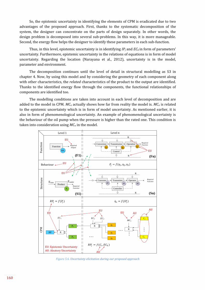
160
So, the epistemic uncertainty in identifying the elements of CPM is eradicated due to two
advantages of the proposed approach. First, thanks to the systematic decomposition of the
system, the designer can concentrate on the parts of design separately. In other words, the
design problem is decomposed into several sub-problems. In this way, it is more manageable.
Second, the energy flow helps the designer to identify these parameters in each sub-function.
Thus, in this level, epistemic uncertainty is in identifying IPj and ECk in form of parameters’
uncertainty. Furthermore, epistemic uncertainty in the relations of equations is in form of model
uncertainty. Regarding the location (Narayana et al., 2012), uncertainty is in the model,
parameter and environment.
The decomposition continues until the level of detail in structural modelling as S3 in
chapter 4. Now, by using this model and by considering the geometry of each component along
with other characteristics, the related characteristics of the product to the output are identified.
Thanks to the identified energy flow through the components, the functional relationships of
components are identified too.
The modelling conditions are taken into account in each level of decomposition and are
added to the model in CPM. MCn actually shows how far from reality the model is. MCn is related
to the epistemic uncertainty which is in form of model uncertainty. As mentioned earlier, it is
also in form of phenomenological uncertainty. An example of phenomenological uncertainty is
the behaviour of the oil pump when the pressure is higher than the rated one. This condition is
taken into consideration using MCn in the model.
Figure 5.6. Uncertainty elicitation during our proposed approach
RP
P1
P2
R
EC2 EC3
Rη1
EC1
η2
η3
R
…
C1
Ci
Fu
nct
ion
Stru
ctu
reC
PM
Behaviour
TransmissionConversion Operation
Control
R
η1 η2
R
Required
Functionη3
Level 1 Level n
Function
RPj
Product
Pj
EinletEoutlet
Required Function
TransmitterConverter Operator
Controller
R
R
Required
Function
IPjIPj IPj
… …
…
𝑃𝑗 = 𝑓(𝜂1 , 𝜂2 ,𝜂3)
𝑅𝑃𝑗 = 𝑓(𝑃𝑗 ) 𝜂𝑒 = 𝑓(𝐼𝑃𝑗 )
𝑅𝑃𝑗 = 𝑓(𝐶𝑖 ,𝐸𝐶𝑘)
Required Output
MCn
EU
EU
EU
AUEU AUEU
EU
AU
EU
EU: Epistemic Uncertainty
AU: Aleatory Uncertainty
(F1)
(S1)
(Fn)
(Sn)
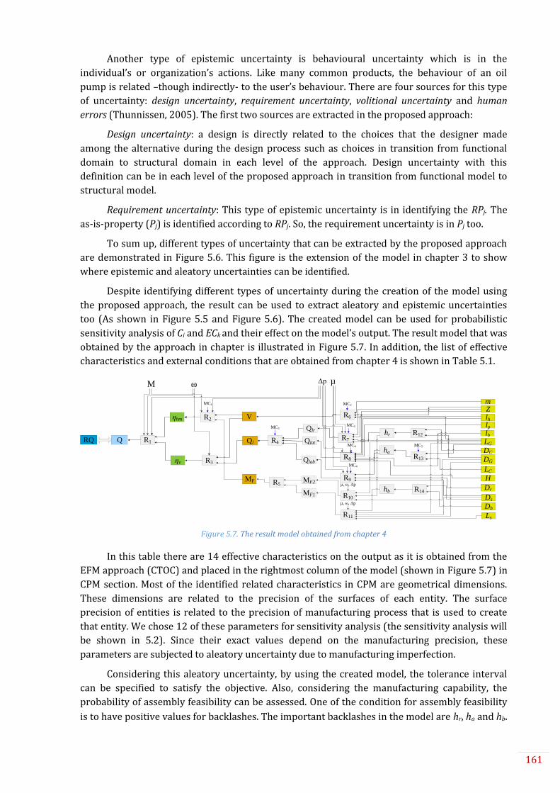
161
Another type of epistemic uncertainty is behavioural uncertainty which is in the
individual’s or organization’s actions. Like many common products, the behaviour of an oil
pump is related –though indirectly- to the user’s behaviour. There are four sources for this type
of uncertainty: design uncertainty, requirement uncertainty, volitional uncertainty and human
errors (Thunnissen, 2005). The first two sources are extracted in the proposed approach:
Design uncertainty: a design is directly related to the choices that the designer made
among the alternative during the design process such as choices in transition from functional
domain to structural domain in each level of the approach. Design uncertainty with this
definition can be in each level of the proposed approach in transition from functional model to
structural model.
Requirement uncertainty: This type of epistemic uncertainty is in identifying the RPj. The
as-is-property (Pj) is identified according to RPj. So, the requirement uncertainty is in Pj too.
To sum up, different types of uncertainty that can be extracted by the proposed approach
are demonstrated in Figure 5.6. This figure is the extension of the model in chapter 3 to show
where epistemic and aleatory uncertainties can be identified.
Despite identifying different types of uncertainty during the creation of the model using
the proposed approach, the result can be used to extract aleatory and epistemic uncertainties
too (As shown in Figure 5.5 and Figure 5.6). The created model can be used for probabilistic
sensitivity analysis of Ci and ECk and their effect on the model’s output. The result model that was
obtained by the approach in chapter is illustrated in Figure 5.7. In addition, the list of effective
characteristics and external conditions that are obtained from chapter 4 is shown in Table 5.1.
Figure 5.7. The result model obtained from chapter 4
In this table there are 14 effective characteristics on the output as it is obtained from the
EFM approach (CTOC) and placed in the rightmost column of the model (shown in Figure 5.7) in
CPM section. Most of the identified related characteristics in CPM are geometrical dimensions.
These dimensions are related to the precision of the surfaces of each entity. The surface
precision of entities is related to the precision of manufacturing process that is used to create
that entity. We chose 12 of these parameters for sensitivity analysis (the sensitivity analysis will
be shown in 5.2). Since their exact values depend on the manufacturing precision, these
parameters are subjected to aleatory uncertainty due to manufacturing imperfection.
Considering this aleatory uncertainty, by using the created model, the tolerance interval
can be specified to satisfy the objective. Also, considering the manufacturing capability, the
probability of assembly feasibility can be assessed. One of the condition for assembly feasibility
is to have positive values for backlashes. The important backlashes in the model are hr, ha and hb.
LG
Zm
ha
V
Ql
ηv
ηhm
R13R3
R2
R4
R6
R1
H
hr
Dr
DC
DG
LC
R12
Ds
lh
Qlr
Qlat
Qlab
R7
R8
R9
ω M
Q
lp
lb
MC1 MC2
MC3MC4
MC4
MC4
MC5
MF
Db
Ls
MF1
MF2R5
R11
R10
hb R14
µ, ω, Δp
µ, ω, Δp
RQ
µ ∆p

162
Looking at the model in Figure 5.7, there are 6 characteristics (DC, DG, LC, LG, Ds, Db) that are
related to these backlashes. So, the values of (DC ‒ DG), (LC ‒ LG) and (Db ‒ Ds) should be positive.
So, aleatory uncertainty in the value of these parameters effect on assembly.
Table 5.1. Uncertain variables and their variation for Monte Carlo Simulation
Parameter Nominal value Unit Variation
Ch
arac
teri
stic
s (C
i)
Z Number of teeth 8 # 0
m Module of the gear tooth 25×10-3/Z m 0
lh Head length of the teeth 1.8×10⁻³ m N(1.8×10⁻³, 3.6×10⁻⁵)
lp Primitive length of the teeth (π/2)m m N(π.m/2, π.m×10-2)
lb Base length of the teeth 9.5×10⁻³ m N(9.5×10⁻³, 19×10-5)
DC Gear casing diameter 56.99×10⁻³ m N(56.99×10⁻³, 113.98×10⁻⁵)
DG Gear diameter 56.50×10⁻³ m N(56.5×10⁻³, 113×10-5) LC Gear casing depth 21.45×10⁻³ m N(21.45×10⁻³, 42.9×10⁻⁵) LG Gear thickness 21.4×10⁻³ m N(21.4×10⁻³, 42.8×10⁻⁵) H Tooth depth 6×10⁻³ m N(6×10⁻³, 12×10-5) Dr Root diameter 19×10-3 m N(19×10-3, 38×10-5) Ds Shaft diameter 10×10-3 m N(10×10-3, 20×10-5) Db Bearing diameter 10.01×10⁻³ m N(10.01×10⁻³, 20.02×10⁻⁵) Ls Shaft length 22×10-3 m N(22×10-3, 44×10-5)
EC
k
µ Fluid dynamic viscosity 19.8×10⁻³ Pa U(18.81×10-3,20.79×10-3)
ΔP Pressure rise 500000 Nm U(475000,525000)
M Input Torque 2.75 rad/s U(2.6125,2.8875)
ω Angular rotation speed 235.619 Pa.s U(223.838,247.4)
The second group of effective parameters are ECk including four parameters of µ, ΔP, M
and ω. A complete identification of these parameters depends on the knowledge of the designer
about the system’s environment and its impact on the system’s function. So, these parameters
are affected by epistemic uncertainty.
Despite the identification of these parameters, their values during the functioning of the
system are not stable. In the studied case, ECk varies in different engine speeds (ΔP, M and ω),
temperatures (µ) and types of oil (µ, ΔP). Also, due to the depreciation, these values change. So,
aleatory uncertainty in ECk occurs too. To consider these types of uncertainty in CPM, sensitivity
analysis is done for the impact of ECk on output (Q) as well.
Thanks to the identified effective parameters (Ci and ECk) and relations among Ci, ECk and
Pj, sensitivity analysis by using algorithm like Monte Carlo Simulation is possible. For this
analysis, as illustrated in Table 5.1, for characteristics (except two parameters that are fixed for
a standard gear) normal distribution with mean equals to the nominal value and standard
deviation of 2% is used to give random values within the accepted intervals. In case of ECk, the
optimistic and pessimistic values are taken into consideration with ±5% interval. In this section
the focus is in uncertainty. In the next section, different types of sensitivity analysis will be
studied by using this information.
For uncertainty elicitation in CPM solution analysis, regarding the upper and lower
probability measure of (Dempster, 1967) and the theory of evidence (Shafer, 1976), the
Cumulative Belief Function (CBF) and Cumulative Plausibility Function (CPF) are calculated. The
identified types of uncertainty in the design process as presented includes epistemic and
aleatory. According to (Guo & Du, 2007) elicitation of uncertainty by these two functions
considers both aleatory and epistemic uncertainty. The result is shown in Figure 5.8. In this

163
diagram, for each amount of Q (the horizontal axis) the difference between lower and upper
probabilities (CBF and CPF) shows the amount of uncertainty. This diagram can be used for
uncertainty propagation.
Figure 5.8. CBF and CPF from the effect analysis for Q
In this analysis, assembly conditions and functioning conditions (to respect the minimum
backlashes for rotating parts) are taken into account. All these analyses are done established on
the identified relations. Although, EFM and the systematic decomposition approach facilitate this
identification, epistemic model uncertainty exists.
So using the created model by CPM, a sensitivity analysis can be done to identify the most
important input variable with aleatory uncertainty. In addition, the importance of epistemic
uncertainty in effective environmental parameters (as ECk) is measured by its effect on the
model output. The following section illustrates the sensitivity analysis.
5.2. Sensitivity analysis
After the determination of the product model in the first phase of the approach, in the
second phase, the model can be used to analyse the system. In the first phase, the effective
parameters are identified. The objective in the second phase is to identify the key characteristics
and to analyse their effect on the output (value).
Sensitivity analysis is defined as the study of how uncertainty in the output of a model can
be attributed to different sources of uncertainty in the model input (Saltelli et al., 2004).
Mathematically, the derivative of 𝜕𝑌𝑗/𝜕𝑋𝑖 of an output 𝑌𝑗 versus an input 𝑋𝑖 can be thought as a
mathematical definition of the sensitivity of 𝑌𝑗 versus 𝑋𝑖 (Saltelli et al., 2008).
Differential sensitivity analysis is the most fundamental technique in sensitivity analysis. In
this method, also known as ‘direct method’, sensitivity coefficient is the ratio of the change in
output to the change in input while all other parameters remain constant (Krieger et al., 1977).
The partials must be recalculated for each change in the base-case scenario (e.g. all parameters
set to their mean value). So, the sensitivity coefficient for an independent variable can be
calculated from the partial derivative of the dependent variable with respect to the independent
variable (Hamby, 1994). Then, this partial derivative can be estimated as Eq. 5.1.
𝛷𝑖 =
%∆𝑌
%∆𝑋𝑖 (5.1)
0.0002 0.0004 0.0006 0.0008
0.85
0.90
0.95
1.00
CPF
CBF
Q (m3/s)

164
According to Hamby (1994), for sensitivity analysis, first the parameters that require
additional research for strengthening the knowledge base and reducing the uncertainty of the
output are determined. The parameters that are insignificant should be identified and
eliminated from the model. Using our proposed approach, the important and insignificant
parameters are identified thanks to the EFM.
Then the inputs that contribute most to output variability are determined. The result of
the approach is a quantitative model that is created in CPM. The model is created based on the
mathematical relationships of the inputs and outputs. So, by utilizing this model, the designer
can identify which parameters are most highly correlated with the output. Finally, the
consequence results of changing inputs on the output by using the sensitivity methods are
determined.
As presented in chapter 3, the result of the approach is a quantitative model that connects
the output to the effective inputs through a mathematical formula as also shown in Eq. 5.2.
𝑃𝑗 = 𝑓(𝐶𝑖, 𝐸𝐶𝑘|𝑀𝐶𝑛) (5.2)
To illustrate how this model can be used for analysis of the impact of parameters on the
output, the case study that is explained in chapter 4 is used. The result of this case study is the
model in Figure 5.7 which identifies the relationship of Eq. 5.3.
𝑄 = 𝑓(𝑚, 𝑍, 𝑙ℎ , 𝑙𝑝, 𝑙𝑏 , 𝐿𝐺 , 𝐷𝐶 , 𝐷𝐺 , 𝐿𝐶 , 𝐻, 𝐷𝑟, 𝐷𝑠, 𝐷𝑏 , 𝐿𝑠, 𝑀, 𝜔, ∆𝑝, 𝜇 | 𝑀𝐶𝑛) (5.3)
By this model, the impact of changes in the characteristics or/and external condition on
the output (Q) can be analysed. So, for sensitivity analysis, Ci and ECk are the inputs.
In this table, the nominal value for dimensions is the mean value of the manufacturing
system’s output of the pump which is obtained from the draft in the Appendix C. The standard
deviation of each characteristic is found and calculated based on the tolerance interval and
quality level table shown in Table 5.2. In our analysis, based on the material and the process of
manufacturing, the internal tolerance level is chosen. The gears in the oil pump are made of
sintered steel with the process of sintering and the casing is made of aluminium by casting. So
the IT6 is chosen for casing and IT8 for the gears. Normal distribution by mean and standard
deviation in Table 5.1 is used for characteristics in calculations.
Table 5.2. The table of tolerance interval based on the level of quality (ISO 286-1:2010)
International Tolerance (IT) Grade TI in micrometre - Nominal dimensions in mm
From 1 3 6 10 18 30 50 80 120 180 250 315 400
To (included) 3 6 10 18 30 50 80 120 180 250 315 400 500
IT5 4 5 6 8 9 11 13 15 18 20 23 25 27
IT6 6 8 9 11 13 16 19 22 25 29 32 36 40
IT7 10 12 15 18 21 25 30 35 40 46 52 57 63
IT8 14 18 18 27 33 39 46 54 63 72 81 89 97
IT9 25 30 36 43 52 62 74 87 100 115 130 140 155
IT10 40 48 58 70 84 100 120 140 160 185 210 230 250
IT11 60 75 90 110 130 160 190 220 250 290 320 360 400
IT12 100 120 150 180 210 250 300 350 400 460 520 570 630
IT13 140 180 220 270 330 390 460 540 630 720 810 890 970

165
For external conditions, an average value for each parameter (as car is in specific
condition by using specific type of oil) is considered. In order to take into account the variability
of the external conditions, uniform distribution for ECk are considered where the nominal value
is the mean value of each parameter as illustrated in Table 5.1.
Thus, in this section, the impact of these inputs on the output (flow [Q] and total efficiency
[ηt]) is analysed. For this analysis Matlab® software is used for calculations.
The two most common types of sensitivity analysis are Local Sensitivity Analysis (LSA)
and Global Sensitivity Analysis (GSA). The following two sub-sections are assigned two these
two types. For each type, it is illustrated how the result of the proposed model, which is a
quantitative model, can be used for sensitivity analysis of the system. In other words, the model
enables the designer to know how the modifications of the input parameters (characteristics)
effect on the output (as-is property).
To generate values based on the input parameters, Monte Carlo Simulation (MCS) is used.
MCS is a computational algorithm in order to obtain numerical results based on repeated
random sampling. This simulation reduces the cost of trial and error. Instead of testing every
product in terms of their exact geometry, in MSC, random variables based on the mean, standard
deviation and given distribution are used to analyse the system.
5.2.1. Local Sensitivity Analysis (LSA)
The first approach is local sensitivity analysis which is derivative based (numerical or
analytical). Mathematically, the sensitivity of the cost function with respect to certain
parameters is equal to the partial derivative of the cost function with respect to those
parameters. The term local refers to the fact that all derivatives are taken at a single point. So, it
is also called One-at-a-time (OAT) sensitivity technique. This technique analyses the effect of one
parameter on the cost function (Y) at a time while keeping the other parameters fixed. This
analysis can also be done by giving a percentage to each parameter (weight) for sensitivity
ranking.
The drawback of this type is that only a small fraction of the design space is explored,
especially when there are many parameters. Also, it does not provide insight about how the
interactions between parameters influence the cost function.
The first local sensitivity analysis method is by observation the trend of output variation
based on the variation of each input. This is not a very precise analysis of the impact. It only
shows if the impact is positive or negative or how is the trend. Of course, it is only applicable for
up to three variables since the graph of more dimensions cannot be plotted. In this section, only
the OAT analysis is done.
By using the input variables and the relations that are obtained by the proposed approach,
Monte Carlo Simulation (MCS) have been done. So, by keeping all the variations equal to zero
except Xi, using MCS, the impact of Xi on the output can be identified using the trend graph. The
set of diagrams in Figure 5.9 shows the local impact of each characteristic on the outlet flow. The
sample number in this analysis is 100,000.
As indicated in Figure 5.9, the first four parameters (m, lh, lp, lb) are related to the gear
teeth. Based on this analysis, increasing in the value of these parameters causes increasing of the
oil flow. Two parameters of DC and DG have negative and positive effect on the flow respectively.
The difference of these parameters is the radial backlash (hr). Two parameters of LC and LG are

166
related to the axial backlash (ha). So, as this analysis shows, decreasing backlashes will result in
increasing Q. In the same way, (Dr – Ds) is the bearing backlash and decreasing this value will
lead to increasing Q. The last four parameters in Figure 5.9 show the impact off the external
conditions on the flow.
Figure 5.9. Graphical local analysis of the Ci and ECk on Q
The second local sensitivity analysis is the variation of the outputs based on the variation
of the effective inputs. As Eq. 5.4 shows, the impact of the variation of characteristics and
external conditions on the flow (Q) and total efficiency (ηt) can be calculated.
𝐿𝑆𝐴𝑖 =𝜎𝑝𝑒𝑟𝑓𝑜𝑟𝑚𝑎𝑐𝑒 𝑖
𝜎𝑇𝑜𝑡𝑎𝑙 𝑝𝑒𝑟𝑓𝑜𝑟𝑚𝑎𝑛𝑐𝑒
→𝜎𝐶𝑖𝜎𝑄 ,𝜎𝐶𝑖𝜎𝜂 ,𝜎𝐸𝐶𝑘𝜎𝑄
,𝜎𝐸𝐶𝑘𝜎𝜂
(5.4)
Table 5.3 is the result of this analysis to identify the impact of the Ci and ECk on the flow
and efficiency. By looking at the table one can say that variation in m causes the highest variation
in the outputs. After that, among the characteristics, those that are related to the backlashes and
flow loss, have the highest effect. Among the external conditions, angular velocity (ω) varies Q
the most and the variation in pressure rise (Δp) has the highest impact on the efficiency.
Table 5.3. Variation impact of the Ci and ECk on Q and η
Characteristic Q SDQ η SDη
m 4.4230e-04 1.55e-06 92.1527% 0.32357
lh 4.4229e-04 5.52e-10 92.1511% 1.15e-05
lp 4.4229e-04 4.54e-12 92.1511% 9.46e-07
lb 4.4229e-04 2.85e-12 92.1511% 5.94e-07 DC 4.4229e-04 2.00e-08 92.1510% 4.16e-03
DG 4.4229e-04 9.75e-08 92.1496% 0.020318
LC 4.4228e-04 1.19e-07 92.1490% 0.024965
LG 4.4229e-04 1.88e-07 92.1502% 0.039347 H 4.4229e-04 1.35e-11 92.1511% 2.81e-06
Dr 4.4229e-04 1.94e-10 92.1511% 4.05e-05 Ds 4.4229e-04 3.02e-10 92.1511% 6.29e-05

167
ΔP 4.4229e-04 1.89e-09 92.1514% 0.19935
M 4.4229e-04 5.48e-17 92.1513% 0.055892
ω 4.4229e-04 4.94e-06 92.1510% 2.03e-03
μ 4.4229e-04 7.46e-08 92.1498% 0.01555 Number of samples = 100 000
After the analysis of the variation of the effective parameters based on the values of the
result of the manufacturing system, next is to give more variations for the inputs to highlight the
effect on the outputs. So, three levels of standard deviation are considered for each parameter.
Each time, the calculation formula is the same as Eq. 5.4. The result of this analysis is gathered in
Table 5.4. In this analysis, three different standard deviations are taken into account for each
characteristic and the effect on the efficiency.
Table 5.4. Analysis of the impact of the characteristics’ variation on ηt by trying three standard deviations
Sample size: 100000
initial value (hi)
σ(Ci) ηt Friction probability
m 33e-5 95.70%
3.125e-3 33e-6 96.46% 33e-8 95.66%
lt4
1.77e-03 92.14% 4.3785e-03 1.77e-05 92.15%
1.77e-07 92.15%
DC 19e-4 96.37% → Radial friction probability = 28.7%
56.99e-3 19e-6 96.45% 19e-08 96.45%
DG 2*(46e-4) 94.29% → Radial friction probability = 47.3%
56.79e-3 2*(46e-6) 96.45% 2*(46e-8) 96.45%
LC 52e-4 94.50% → Axial friction probability = 45.8%
21.5e-3 52e-6 96.45% 52e-8 96.45%
LG 33e-4 95.34% → Axial friction probability = 44%
21.4e-3 33e-6 96.45% 33e-8 96.45%
H 22e-4 96.45%
6e-3 22e-6 96.45% 22e-8 96.45%
Dr 33e-4 96.45%
19e-3 33e-6 96.45% 33e-8 96.45%
Ds 27e-4 96.45%
10e-3 27e-6 96.45% 27e-8 96.45%
Base on the result of the sensitivity analysis, parameters of DC, DG, LC and LG are related
to the distance of the gears and the casing. A minimum gap is necessary for the rotation of the
pinions in the casing. If the minimum is not satisfied, friction happens. Thus, the probability of
the friction between the pinions and the casing is calculated too. As Table 5.4 shows, in four
cases, the friction probability is too high to be accepted based on the level of quality. So, the
corresponding σi are not accepted.
The next analysis is by changing the mean value of the characteristics and analyse the
impact on the outputs (Eq. 5.5). The result is shown in Table 5.5.
4 Instead of three parameters of lh, lp and lb which are related to the pinion teeth, lt is used which is
calculated as : lt = 3√(lh.lp.lb)
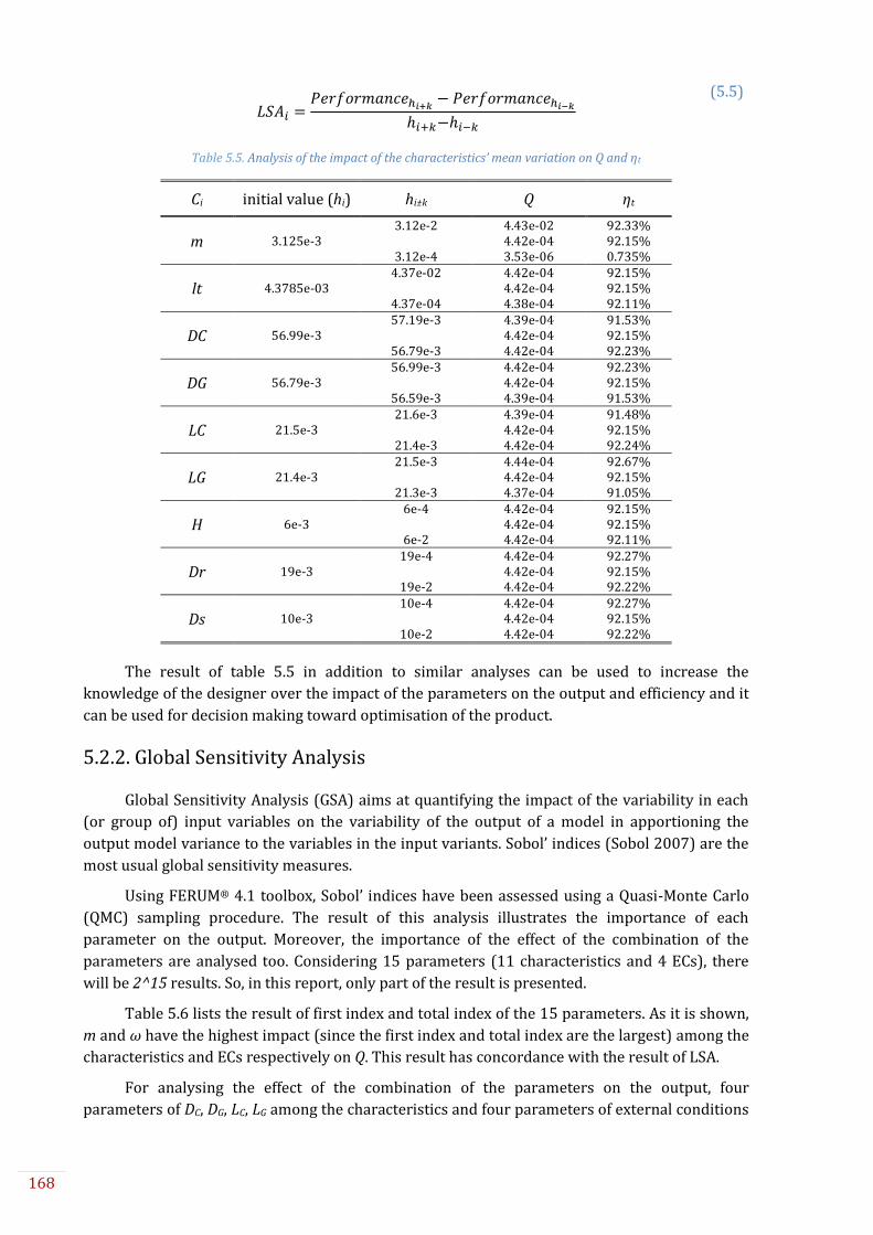
168
𝐿𝑆𝐴𝑖 =
𝑃𝑒𝑟𝑓𝑜𝑟𝑚𝑎𝑛𝑐𝑒ℎ𝑖+𝑘 − 𝑃𝑒𝑟𝑓𝑜𝑟𝑚𝑎𝑛𝑐𝑒ℎ𝑖−𝑘ℎ𝑖+𝑘−ℎ𝑖−𝑘
(5.5)
Table 5.5. Analysis of the impact of the characteristics’ mean variation on Q and ηt
Ci initial value (hi) hi±k Q ηt
m 3.12e-2 4.43e-02 92.33%
3.125e-3 4.42e-04 92.15% 3.12e-4 3.53e-06 0.735%
lt 4.37e-02 4.42e-04 92.15%
4.3785e-03 4.42e-04 92.15% 4.37e-04 4.38e-04 92.11%
DC 57.19e-3 4.39e-04 91.53%
56.99e-3 4.42e-04 92.15% 56.79e-3 4.42e-04 92.23%
DG 56.99e-3 4.42e-04 92.23%
56.79e-3 4.42e-04 92.15% 56.59e-3 4.39e-04 91.53%
LC 21.6e-3 4.39e-04 91.48%
21.5e-3 4.42e-04 92.15% 21.4e-3 4.42e-04 92.24%
LG 21.5e-3 4.44e-04 92.67%
21.4e-3 4.42e-04 92.15% 21.3e-3 4.37e-04 91.05%
H 6e-4 4.42e-04 92.15%
6e-3 4.42e-04 92.15% 6e-2 4.42e-04 92.11%
Dr 19e-4 4.42e-04 92.27%
19e-3 4.42e-04 92.15% 19e-2 4.42e-04 92.22%
Ds 10e-4 4.42e-04 92.27%
10e-3 4.42e-04 92.15% 10e-2 4.42e-04 92.22%
The result of table 5.5 in addition to similar analyses can be used to increase the
knowledge of the designer over the impact of the parameters on the output and efficiency and it
can be used for decision making toward optimisation of the product.
5.2.2. Global Sensitivity Analysis
Global Sensitivity Analysis (GSA) aims at quantifying the impact of the variability in each
(or group of) input variables on the variability of the output of a model in apportioning the
output model variance to the variables in the input variants. Sobol’ indices (Sobol 2007) are the
most usual global sensitivity measures.
Using FERUM® 4.1 toolbox, Sobol’ indices have been assessed using a Quasi-Monte Carlo
(QMC) sampling procedure. The result of this analysis illustrates the importance of each
parameter on the output. Moreover, the importance of the effect of the combination of the
parameters are analysed too. Considering 15 parameters (11 characteristics and 4 ECs), there
will be 2^15 results. So, in this report, only part of the result is presented.
Table 5.6 lists the result of first index and total index of the 15 parameters. As it is shown,
m and ω have the highest impact (since the first index and total index are the largest) among the
characteristics and ECs respectively on Q. This result has concordance with the result of LSA.
For analysing the effect of the combination of the parameters on the output, four
parameters of DC, DG, LC, LG among the characteristics and four parameters of external conditions
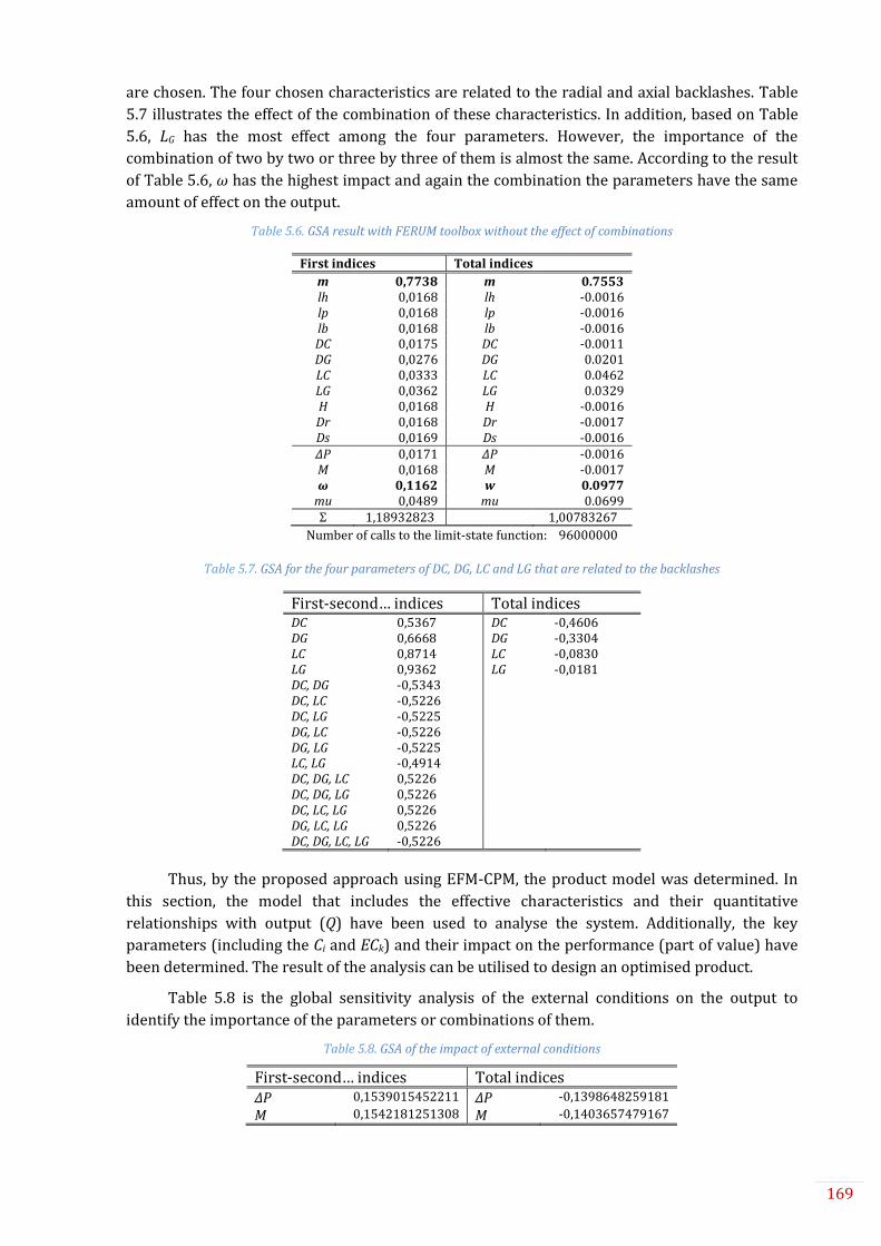
169
are chosen. The four chosen characteristics are related to the radial and axial backlashes. Table
5.7 illustrates the effect of the combination of these characteristics. In addition, based on Table
5.6, LG has the most effect among the four parameters. However, the importance of the
combination of two by two or three by three of them is almost the same. According to the result
of Table 5.6, ω has the highest impact and again the combination the parameters have the same
amount of effect on the output.
Table 5.6. GSA result with FERUM toolbox without the effect of combinations
Number of calls to the limit-state function: 96000000
Table 5.7. GSA for the four parameters of DC, DG, LC and LG that are related to the backlashes
First-second… indices Total indices DC 0,5367 DC -0,4606 DG 0,6668 DG -0,3304 LC 0,8714 LC -0,0830 LG 0,9362 LG -0,0181 DC, DG -0,5343 DC, LC -0,5226 DC, LG -0,5225 DG, LC -0,5226 DG, LG -0,5225 LC, LG -0,4914 DC, DG, LC 0,5226 DC, DG, LG 0,5226 DC, LC, LG 0,5226 DG, LC, LG 0,5226 DC, DG, LC, LG -0,5226
Thus, by the proposed approach using EFM-CPM, the product model was determined. In
this section, the model that includes the effective characteristics and their quantitative
relationships with output (Q) have been used to analyse the system. Additionally, the key
parameters (including the Ci and ECk) and their impact on the performance (part of value) have
been determined. The result of the analysis can be utilised to design an optimised product.
Table 5.8 is the global sensitivity analysis of the external conditions on the output to
identify the importance of the parameters or combinations of them.
Table 5.8. GSA of the impact of external conditions
First-second… indices Total indices ΔP 0,1539015452211 ΔP -0,1398648259181
M 0,1542181251308 M -0,1403657479167
First indices Total indices
m 0,7738 m 0.7553 lh 0,0168 lh -0.0016 lp 0,0168 lp -0.0016 lb 0,0168 lb -0.0016 DC 0,0175 DC -0.0011 DG 0,0276 DG 0.0201 LC 0,0333 LC 0.0462 LG 0,0362 LG 0.0329 H 0,0168 H -0.0016 Dr 0,0168 Dr -0.0017 Ds 0,0169 Ds -0.0016 ΔP 0,0171 ΔP -0.0016 M 0,0168 M -0.0017 ω 0,1162 w 0.0977
mu 0,0489 mu 0.0699 Σ 1,18932823 1,00783267

170
ω 1,0504846846105 ω 0,7559008115511
μ 0,2435982664505 μ -0,0501681046920
ΔP, M -0,1542181251309
ΔP, ω -0,1542181251395
ΔP, μ -0,1534006232225
M, ω -0,1542181251310
M, μ -0,1542181251313
ω, μ -0,1542181251425
ΔP, M, ω 0,1542181251310
ΔP, M, μ 0,1542181251310
ΔP, ω, μ 0,1542181251390
M, ω, μ 0,1542181251310
ΔP, M, ω, μ -0,1542181251299
5.3. Tolerance analysis
The third section of this chapter explains how the approach and the obtained result can
give a runway to the designer for tolerance analysis. In fact, the applicability of the approach in
tolerance analysis is an extension of its applicability in sensitivity analysis that has been
explained in the previous section.
As mentioned in chapter 1, the objective of this thesis is to improve the Value. Value has
been defined in two axes of quality and cost. In our approach the quality of a product is related
to its efficiency. Efficiency is related to the losses in the system. So, if different losses are
reduced, the efficiency can be increased. In many cases, the losses are related to the gaps
between moving parts, assembled parts or any other gaps that are necessary and unavoidable or
avoidable in functioning of the product. Any backlash is related to the dimensions of two or
more parts. This backlash variation can be controlled by limitation of tolerances. Therefore,
taking into account the liaison between efficiency and tolerances, one of the approaches to
improve product quality is tightening tolerances. In this approach, the key point is to find the
related tolerances to the performance of the product.
The second axis is cost. Tightening the tolerances means having smoother surfaces of the
parts. So, the precision of the manufacturing process should be increased. Increasing in the
precision requires modifying the manufacturing steps, increasing machine capability, more
accurate tools, more skilled operators etc. These improvements increase the cost of
manufacturing.
Thus, tightening tolerances leads to increase the quality and higher cost. Some
manufacturers prefer to have low cost of manufacturing even though the result is not a premium
product. Though, other manufacturers prefer better products even if it would increase the cost
and therefore the price of the product. So, a balance needs to be achieved between these two
axes and it is not necessary the same for all manufacturers. However, the question is the same
for all: “Does the level of quality worth the cost?”.
To answer this question, the approach to model a system in concurrent designing will be
presented in chapter 6. In this chapter, the quality-tolerance aspect is focused. Thanks to the
proposed approach, EFM-CPM creates a link between quality and structure and therefore
between performance and tolerances. In the following sub-sections, it is shown how integrating
tolerancing in the proposed approach can help the designer in uncertainty management and
reducing complexity.
5.3.1. Context

171
Tolerancing has an essential role in design and manufacturing. As it is also shows in Figure
5.10 dimensions and tolerances influence almost all aspects of the product development through
the product life cycle (Dantan, 2014; Hong & Chang, 2002).
Figure 5.10. Ubiquitous role of tolerances in a product life cycle (Hong & Chang, 2002)
Commonly, there are four aspects of tolerancing: Tolerance representation, tolerance
specification, tolerance analysis, and tolerance synthesis (Dantan, 2014; Salomons, van Houten,
& Kals, 1998). Here, the focus is in the aspect of tolerance specification which is to identify the
related tolerances to the performance and function of the system. Several approaches are
presented in literature for this aspect (Desrochers & Laperrière, 2003; Johannesson &
Soderberg, 2000; Mathieu & Marguet, 2001; U. Roy, Pramanik, Sudarsan, Sriram, & Lyons, 2001).
The determined relations in these approaches are qualitative. So, two aspects of tolerance
analysis and synthesis are used to have a quantitative model of system based on the identified
qualitative links. Moreover, Dantan, Anwer, & Mathieu (2003) proposed a multi-level approach,
which includes parallel processes of conceptual design and tolerancing process as shown in
Figure 5.11.
In these approaches, the designer studies the functional performance of a product and
then looks for geometrical requirement that might effect on the performance. Then, based on the
geometrical requirements, the related tolerances are identified. So, in tolerance analysis, the
designer needs to model the functional characteristics, component deviations, and
environmental impacts. So, both qualitative and quantitative relations should be in the system’s
model.
Thus, the designer first needs to find the link between system’s function and its
specifications. Second, the impact of related tolerances to each specification is analysed on the
performance of the system. The difficulty is to link the qualitative functional requirements to the
quantitative functional tolerances. So, a multi-physical approach is needed to assure the
transition from function to tolerances taking into account both qualitative and quantitative
aspects.
The proposed approach creates a quantitative link between functional performance and
functional tolerances. In this approach the qualitative functional and tolerance requirements are
combined with quantitative relations. As mentioned, the approach includes two phases. The first
phase, which has been explained in chapter 3, is to create a quantitative model of the product
based on the functional performance, behaviour and structure of the product. The model
establishes a link between functional performance and geometrical dimensions. In the second

172
phase, which is in this chapter, the model is used to analyse the impact of tolerances on
functional performance. So, in this section, it will be explained, how the second phase of the
approach can be used in tolerance analysis.
Figure 5.11. Common approach for function-tolerance analysis (Dantan et al., 2003)
5.3.2. Using the proposed approach in tolerancing
As in sensitivity analysis, the result of the modelling phase which is Eq. 5.2 is applied for
tolerance analysis. As illustrated in section 5.2, thanks to this equation, which is the combination
of the relationships in CPM, one can evaluate the impact of characteristics and external
conditions on the system’s performance. An important group of characteristics in CPM created
by the proposed approach is parts’ geometrical dimensions. These dimensions are the result of
manufacturing process. So, based on the precision of manufacturing process, different tolerance
intervals can be assigned to each Ci as shown in Eq. 5.6.
𝑃𝑗 = 𝑓(𝐶𝑖) 𝑤ℎ𝑒𝑟𝑒 𝑔(𝐶𝑖) ≤ 𝑇𝐼𝑖 (5.6)
In tolerancing point of view, lower precision of process will lead to higher tolerance
interval of these two parameters. Higher tolerance interval means there are more chances of
having product with flow loss higher than accepted. So, there is higher probability of low-quality
products.
Eq. 5.2 is also containing the impact of external conditions (ECk) on the output of the
system. To consider the behaviour of a system, the impact of environmental effects on the
system should be considered as well. By having ECk in the relations of CPM, these effects are
considered in the modelling phase. In analysis phase (phase 2), the impact of these parameters
can be assessed like the impact of Ci. For instance, type of oil used in the oil pump might effect on
Q. As shown in sensitivity analysis oil viscosity (µ) has a direct relationship with oil flow (Q).
Requirement
Function
Behavior
Structure
Decomposed function
Geometrical requirement
Functional tolerance
Conceptual design Tolerancing process
Function, Structure
Geometrical constraints
GeometryTolerance
...
Detail design

173
Unlike Ci, variation of ECk is mostly during the operation of the system. So it is part of the
system’s behaviour. In comparison with Cis, the value of these parameters varied in larger
intervals. So analysis of ECk in phase 2 is important to assure the correct functioning of the
system in different environmental conditions.
The second applicability of the approach in tolerancing is related to the modelling
condition (MCn). All the analyses in phase 2 depend on the modelling conditions which have
been defined by the designer in modelling phase. So, it is important to analyse the probability of
respecting MC as well as the impact of MC on the performance of the system’s model.
MC is to simplify the modelling process or to concentrate on the objective of modelling.
However, it is important not to consider conditions that cause elimination of an important
aspect of the system. Using Eq. 5.7 and Eq. 5.8, the modelling conditions should be verified.
𝑃𝑟𝑜𝑏𝑎. (𝑀𝐶𝑛) ≥ 𝑋 (5.7)
𝑃𝑟𝑜𝑏𝑎. [𝑓(𝐶𝑖, 𝐸𝐶𝑘) ≥ 𝑌|𝑀𝐶𝑛] (5.8)
Eq. 5.7 calculates the probability of respecting specific MC. So X is related to the
probability of the hypothesis. Eq. 5.8 is the probability of having the required performance while
respecting the specific MC. Therefore, Y is related to the impact of hypothesis on the
performance of the system. X and Y in Eq. 5.7 and Eq. 5.8 are defined by the client and/or the
designer. Several examples of tolerance analysis and probability analysis are presented here.
One of the examples of modelling condition in discussed case study is:
MC3: External leakage (EL) is considered as zero.
This condition considers zero tolerance for the surface between two parts of pump casing
(CPHF and CRPH). To verify if this condition is negligible, the probability of MC3 as shown in Eq.
5.9 is calculated.
𝑃𝑟𝑜𝑏𝑎. (𝑀𝐶3) = 1 − 𝑃𝑟𝑜𝑏𝑎. (𝐸𝐿 = 0) = 0.99988 (5.9)
This value is obtained by testing the final product. 12 rejected products out of 100,000
products due to external leakage is an acceptable number for the client to verify MC3. Another
example is MC1: “There is no friction between gears’ teeth and casing.”
This statement means first, the backlash between gears and casing should be more than
zero to make the assembly possible. Negative backlash (gear’s diameter more than the space
containing the gear) might happen after manufacturing of the components and before the
assembly.
Second, the backlash should be more than a specific amount to avoid friction. During
product functioning, because of out-of-round of the gear shaft, asymmetrical manufactured
gears, or/and rough surfaces, friction happens. So, since the designer considered this condition
in modelling process to simplify equations, it should be verified. So;
𝑃𝑟𝑜𝑏𝑎. (𝐸𝑎𝑠𝑦 𝑎𝑠𝑠𝑒𝑚𝑏𝑙𝑦) = 𝑃𝑟𝑜𝑏𝑎. (𝐵𝑎𝑐𝑘𝑙𝑎𝑠ℎ > 0) = 0.9831 (5.10)

174
𝑃𝑟𝑜𝑏𝑎. (𝑁𝑜 𝐹𝑟𝑖𝑐𝑡𝑖𝑜𝑛) = 𝑃𝑟𝑜𝑏𝑎. (𝐵𝑎𝑐𝑘𝑙𝑎𝑠ℎ > 0.001 𝑚𝑚) = 0.9824 (5.11)
Eq. 5.10 as the probability of “easy assembly” is calculated. This means if the backlash is
greater than zero, the assembly is possible. Eq. 5.11 is the possibility of friction during
functioning of the product. Regarding the causes for friction, the value of 0.001 mm is chosen as
the minimum backlash to avoid friction.
𝑃𝑟𝑜𝑏𝑎. (𝑄 ≥ 0.0008𝑚3
𝑠⁄ |𝐸𝑎𝑠𝑦 𝑎𝑠𝑠𝑒𝑚𝑏𝑙𝑦) = 0.9791 (5.12)
𝑃𝑟𝑜𝑏𝑎. (𝑄 ≥ 0.0008𝑚3
𝑠⁄ |𝑁𝑜 𝑓𝑟𝑖𝑐𝑡𝑖𝑜𝑛) = 0.9783 (5.13)
The objective in this case study is having specific oil flow (Q) as output. So, the impact of
these modelling conditions is verified according to the minimum acceptable Q (48 l/min). These
probabilities are shown in Eq. 5.12 and Eq. 5.13.
It is up to the designer and client to accept the modelling condition based on the result of
Eq. 5.10 – Eq. 5.13. Their decision is based on the objective and precision of the model.
In product design process, identifying the link between functional requirement and the
specification of a product is an important issue. The presented systematic approach creates a
pathway for designer from functional requirements to the product characteristics and their
specifications.
Figure 5.12 is based on the schema of our approach compared to Figure 5.11. As this figure
shows, energy flow enables the transition from functional performance to functional structure.
After a multi-physical modelling of the behaviour of the system using energy flow, the model is
created in the template of CPM. Thus the model demonstrates the function-behaviour-structure
link. By this link, the analysis of functional tolerance is possible.
So compared to the common approaches, in our approach, the qualitative and quantitative
approaches are combined and the tolerancing process is integrated in design approach. The
function decomposition is done in energy flow approach. Geometrical requirements are taken
into account in structure modelling using characteristics dependencies in CPM. In this approach
only functional tolerances are taken into account. So, the designer can start the detail design
with knowledge over the minimum requirements of the system.
This approach gives a better perspective for creating a new product or studying an existed
product. For creating a new product, the approach begins with the required function and
decomposes the requirements. Therefore, the designer can deal with smaller and more
manageable design problems. Structural decisions are made step by step systematically. So, it
reduces the uncertainty in decision making.
If the product exists, this approach can be used to improve the product. By identifying the
necessary components of the system, unnecessary costly components (or entities) can be
identified. Thanks to the created relationships, changing of properties by modification of
geometrical dimension is possible. Dimensions are limited by related tolerances. Thus, the link
between functional performance and functional tolerances can be established.

175
In analysis phase of the proposed approach, the impact of tolerances on performance of
product can be evaluated. By applying the approach of chapter 6 and combining tolerance-cost
analysis, the result of this evaluation can help the designer to see if tightening a specific
tolerance is worth the cost compared to performance improvement.
Figure 5.12. Our approach compared to common approach
5.4. Conclusion
This chapter illustrated the application of the proposed approach in three areas:
Uncertainty management, sensitivity analysis, tolerance analysis.
In the first section, toward uncertainty management, it was shown how the approach can
help the designer for elicitation of uncertainty. The approach includes two phases. Phase 1 is the
creation of the model using the approach and phase 2 is the analysis of the solution. So,
uncertainty elicitation was done in both phases.
In the first phase, different types of epistemic uncertainty can be identified using the
proposed approach for system model creation. These types are model uncertainty,
phenomenological uncertainty, ambiguity uncertainty and uncertainty in interactions. In the
second phase, both aleatory and epistemic uncertainties are identified and extracted through the
model. So, in the second phase, aleatory uncertainty in characteristics, along with epistemic
uncertainty in environmental impact, model and interaction by using ECk, MCn and Rm
respectively are exploited.
Regarding the classification of Figure 5.1, the drawback of this approach is to identify the
ambiguity uncertainty and behavioural uncertainty. The approach begins according to the
required function of the system. So, due to ambiguity uncertainty in customer needs, it does not
assure that the required function is exactly the customer need. Moreover, regarding the
Requirement
Function
Behavior
Structure
Decomposed function
Geometrical requirement
Functional tolerance
Conceptual design Tolerancing process
Function, Structure
Geometrical constraints
GeometryTolerance
...
Detail design
CPM
Energy flow
Energy flow

176
behavioural uncertainty, the approach only considers the designer’s decisions during the design
process but it can also be due to the uncertainty in user’s interaction with the system or human
errors while using the product. This work has been published in (Malmiry, Dantan, Antoine, &
Pailhès, 2016).
Another application of the proposed approach toward uncertainty management is to
reduce epistemic uncertainty in design process. This part of the work is published in (Malmiry,
Pailhès, et al., 2016) to show how the approach can help the designer to manage complexity that
is due to epistemic uncertainty.
The second section of this chapter is to use the result of the approach for sensitivity
analysis of the system. Thanks to the mathematical relation that the approach creates between
the function and structure, sensitivity analysis can be done using various types of sensitivity
analysis methods. Two types of local and global sensitivity have been used in this chapter. So,
the impact and importance of the effective characteristics of the system on the output
(performance) has been analysed. The most important characteristic is pinion’s tooth module
(m) and the most important EC is rotational velocity (ω). The impact of these two parameters
along with other parameters has been identified. So, this section focused on the phase 2 of the
approach.
The third section of the approach is also part of phase 2 which is tolerance analysis. This
analysis which can be considered as an extension of the second section (sensitivity analysis)
focuses on how the tolerances of characteristics can effect on the system’s performance.
Considering that the majority of the characteristics are geometrical dimensions, by using the
proposed approach, a link between the functional tolerances and the performance can be
created. This analysis is published in (Malmiry, Dantan, Pailhès, & Antoine, 2016b).
As illustrated, not only the result of the approach can be used for sensitivity analysis
focusing on tolerancing (tolerance analysis), the approach creates a pathway for the designer to
move from conceptual design to functional tolerances (tolerance synthesis). Moreover, the
functional, behavioural and structural descriptions of the system are taken into account. Apart
from that, the advantage of this approach compared to similar approaches is that the result
considers both qualitative and quantitative aspects.

177

178
CHAPTER 6
1) LR: Concurrent design
2) LR: Complexity
3) LR: DTMs
4) Choosing the best
5) Creation of the Product design approach
6) Repetition of step 3 and 4.
7) Experimentation: Product design approach
8) Experimentation: Product design approach on another case study
9) Improvement of the product design approach
10) Concurrent design approach
11) Experimentation: Concurrent design approach
12) Modification on the product approach for concurrent design.
13) Sensitivity analysis
14) Uncertainty management
15) Tolerance optimisation
16) Conclusion
6. IPPM
5. Uncertainty & Complexity management
4. Case study
3. Product
2. Literature Review
1. Introduction
1.1. Context
1.2. Research questions
1.3. Research objectives
1.4. Methodology
1.5. Thesis outline
2.1. Context
2.2. Value
2.3. Concurrent designing
2.4. Complexity
2.5. DTM
3.1. Context
3.2. Extended-CPM
3.3. Energy flow modelling
3.4. Product modelling approach
3.5. Mini case study
4.1. Oil pump
4.2. Product model
4.3. Complementary tools
5.1. Uncertainty management
5.2. Sensitivity analysis
5.3. Tolerance analysis
6.1. Context
6.2. Flows
6.3. CPM in IPPD
6.4. IPPM approach
6.5. Case study
6.6. Tolerance optimisation
Research questions
1. How concurrent designing can profit industry and how to assess value in this concept?
2. What are the sources of complexity in IPPD and how to manage them?
3. How to manage design uncertainty?
4. How to model an integrated product/process system systematically to increase �value ?
5. How the model can be used to analyse and optimise the system?
M e t h o d o l o g y
Conclusion

179
CHAPTER 6:
A Modelling Proposition for Integrated
Product/Process Design
In this chapter, an approach is presented for modelling in concurrent designing environment. The
global objective in concurrent designing is to increase the value. As defined in chapter 1 and 2,
value includes two axes of quality and cost. Focusing on the quality (performance) an approach has
been proposed in chapter 3 for modelling a product. In order to consider the second axis (Cost),
concurrent modelling of product and its process is used. The aim of this approach is to help the
designer making decisions in each level of decomposition while considering both aspects.
First, an approach is proposed for modelling the process of manufacturing. In order to have a
systematic approach for concurrent designing, the same framework as product approach (chapter
3) should be used. So, CPM is used as the framework of the approach for process modelling too.
Instead of energy flow, the flow of material and information is used for identifying the elements of
CPM and transition from function to structure. In process, function is the total cost of
manufacturing and structure is all the modifiable parameters that effect on the total cost. In
addition, productivity and risk should also be included in the modelling process. Therefore, in CPM
ontology, as-is- properties are cost and productivity, and the time, capability and other modifiable
process parameters are the characteristics.
Having the same framework and strategy generates the possibility of using this model in
concurrent designing. So, by combining these two models, one can design or optimise a system in
terms of both quality and cost. As before, in each level of decomposition, the functional model is
created and according to that the decisions regarding the structural model are made. The
difference is that in concurrent design, the decisions are made with consideration of the cost. So, the
approach includes four domains: functional, structural, process and CPM. CPM includes a model for
process as well as for product. In this chapter, to avoid confusion and since it is presented in
chapter 3 and 4, only process model is demonstrated. For better demonstration of the approach, the
same case study as chapter 3 (the oil pump) is used by extending the product modelling approach
to concurrent modelling approach.

180
6.1. Context
In order to have a modelling approach for concurrent design, a common framework and a
similar tool are required. Feng & Song (2000) propose an approach for integration of conceptual
design and process planning. In addition they propose various tools that can be utilised in each
level of this approach. This integration is illustrated in Figure 6.1. In the product domain, a
similar approach as we proposed in chapter 3 is used except the links are only qualitative. In the
same way, in the conceptual process planning domain, process, equipment/skill, time and cost
should be taken into consideration. With aiming at identifying both qualitative and quantitative
links between the process elements, these steps should be integrated in the proposed approach.
Process selection and resource selection are parts of decisions that should be made during the
design process. Time and cost estimations are the factors that affect the decisions regarding the
choices in both product and process design. All these aspects in process design need to be added
to the product design requirements to have both high quality and low cost.
Figure 6.1. Integration of conceptual design and process planning (Feng & Song, 2000)
Thus, in this chapter, in a systematic approach, all these considerations will be taken into
account. With the links between product and process elements that are identified with this
approach, it can help the designer to make decisions in each step of design for both product and
process design.
6.2. Flows in product and process
In Integrated Product/Process Design (IPPD), there are two groups of flows: product flows
and process flows. Product flows have been discussed in chapter 3. The flows that could be used
for modelling a mechanical product were signal, material and energy. Energy flow was used to
model the behaviour of the product and identify the CPM elements. The combination of CPM and
EFM in a systematic zigzag approach made the possibility of transition from function to
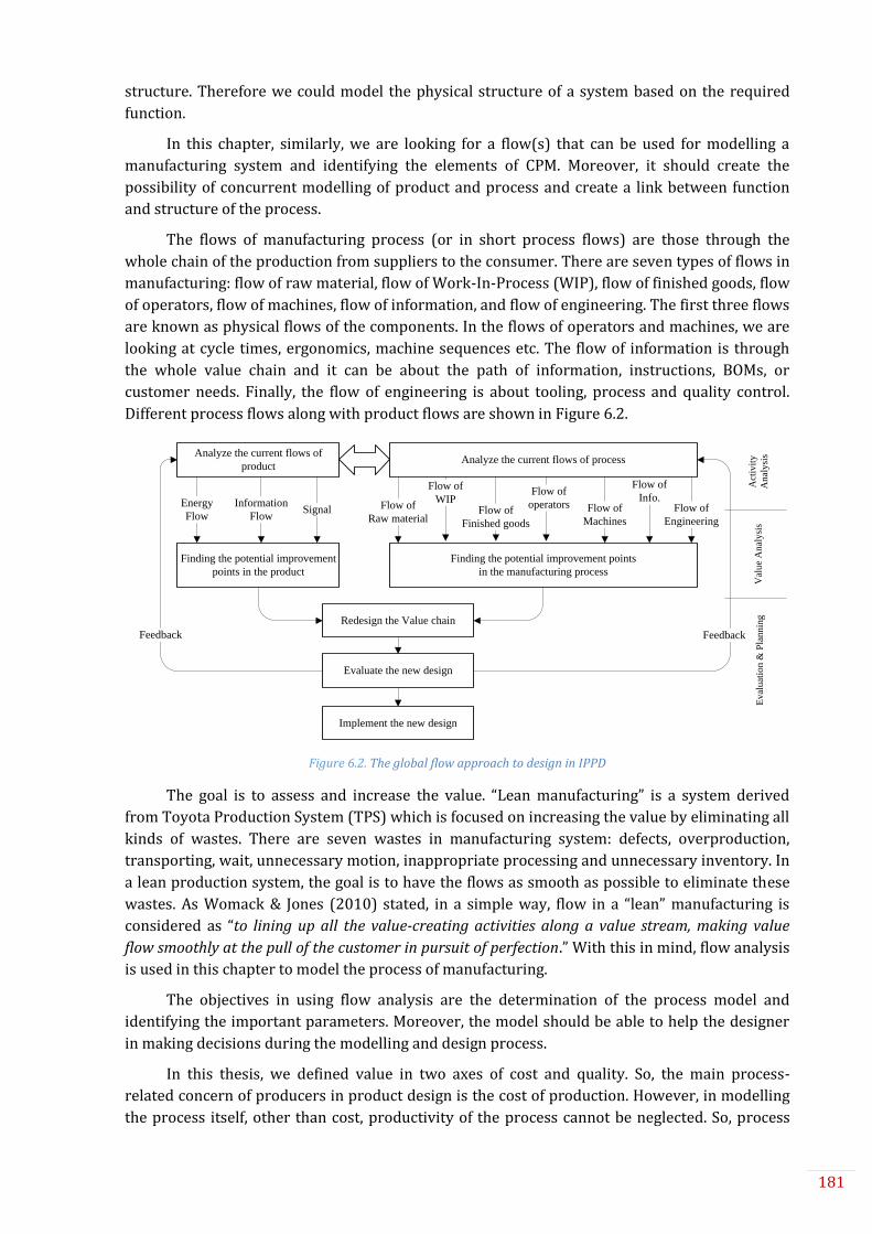
181
structure. Therefore we could model the physical structure of a system based on the required
function.
In this chapter, similarly, we are looking for a flow(s) that can be used for modelling a
manufacturing system and identifying the elements of CPM. Moreover, it should create the
possibility of concurrent modelling of product and process and create a link between function
and structure of the process.
The flows of manufacturing process (or in short process flows) are those through the
whole chain of the production from suppliers to the consumer. There are seven types of flows in
manufacturing: flow of raw material, flow of Work-In-Process (WIP), flow of finished goods, flow
of operators, flow of machines, flow of information, and flow of engineering. The first three flows
are known as physical flows of the components. In the flows of operators and machines, we are
looking at cycle times, ergonomics, machine sequences etc. The flow of information is through
the whole value chain and it can be about the path of information, instructions, BOMs, or
customer needs. Finally, the flow of engineering is about tooling, process and quality control.
Different process flows along with product flows are shown in Figure 6.2.
Analyze the current flows of
productAnalyze the current flows of process
Finding the potential improvement
points in the product
SignalEnergy
FlowFlow of
Finished goods
Finding the potential improvement points
in the manufacturing process
Flow of
Machines
Flow of
Raw material
Flow of
WIPFlow of
operators
Flow of
Info.Flow of
Engineering
Redesign the Value chain
Evaluate the new design
Feedback Feedback
Implement the new design
Information
Flow
Act
ivit
y
Anal
ysi
sV
alue
Anal
ysi
sE
val
uat
ion &
Pla
nnin
g
Figure 6.2. The global flow approach to design in IPPD
The goal is to assess and increase the value. “Lean manufacturing” is a system derived
from Toyota Production System (TPS) which is focused on increasing the value by eliminating all
kinds of wastes. There are seven wastes in manufacturing system: defects, overproduction,
transporting, wait, unnecessary motion, inappropriate processing and unnecessary inventory. In
a lean production system, the goal is to have the flows as smooth as possible to eliminate these
wastes. As Womack & Jones (2010) stated, in a simple way, flow in a “lean” manufacturing is
considered as “to lining up all the value-creating activities along a value stream, making value
flow smoothly at the pull of the customer in pursuit of perfection.” With this in mind, flow analysis
is used in this chapter to model the process of manufacturing.
The objectives in using flow analysis are the determination of the process model and
identifying the important parameters. Moreover, the model should be able to help the designer
in making decisions during the modelling and design process.
In this thesis, we defined value in two axes of cost and quality. So, the main process-
related concern of producers in product design is the cost of production. However, in modelling
the process itself, other than cost, productivity of the process cannot be neglected. So, process

182
cost (PC) and process productivity (PP) are taken as the main parameters (as-is properties) for
process model. These two Pj are added to the Pj of product model which was performance to
have both axes of cost and quality.
A majority of flows in a process as shown in Figure 6.2 are related to material. These flows
are flow of raw material, flow of WIP and flow of finished good. These flows create links between
the machines, operators, operations and inventories. So, material flow is used to model the
process system.
In addition to material flow, information flow is employed for calculation of cost and
productivity. Information flow can be referred to different types of information. Here, the
information about the time of operations, frequency of maintenance, frequency of goods’ import,
availability of operators, … are studied in information flow analysis.
Thus, for process modelling approach, material flow and information flow (denoted as
MF/IF) are used to model the process in CPM and help the designer in decision making process.
The proposition of this chapter is an approach based on MF/IF in the framework of CPM to
create the model of process in a concurrent designing environment and to help the designer in
decision making in a systematic approach.
6.3. CPM in Concurrent designing
In IPPD, there is a two-way relationship between the elements of product and process. In
other words, there are requirements in the process that should be satisfied in the product design
and vice versa. For instance, in product design manufacturability requirements and cost of
production should be considered while in process design the structure of the product regarding
the satisfaction of the function should be taken into account. The links between product and
process in addition to the links in product and process itself create complexity as discussed in
chapter 1. So, in this chapter we propose an approach for modelling product and process that
can help the designer to reduce complexity.
As indicated in the literature review, CPM was presented by Weber for product modelling.
In Integrated Product/Process Modelling (IPPM), we propose to use CPM as the framework for
process modelling too. Using the same framework and similar systematic approach, we create
coherence between product and process.
In this case, there are elements of Ci, Pj, IPj, ECk, MCn and relationships (Rij) for each model
of product and process. So, there is a model of process in CPM as well as one model of product. In
modelling of each product and process, relationships should be identified. However in IPPM, in
addition to the relationships of each model, there are links between the elements of product
with the elements of process. These links are due to the requirements of each domain. These
links are between different types of CPM elements of each model; for instance between Ci of
product and Pj of process or between Ci of process and ECk of product.
Different types of links are discussed here shortly. To demonstrate the links, in each
model, a box that represents a part of model and contains the relations (Rij) is illustrated. As
described in the proposed product modelling approach, the modelling is begun from the
function (RPj and Pj) and models the product until the structure (Ci). So, the inputs for this box
are the properties that are defined based on the requirements. The outputs are the
characteristics since they are related to the structure of the product/process and in other words
it is the result of the design.
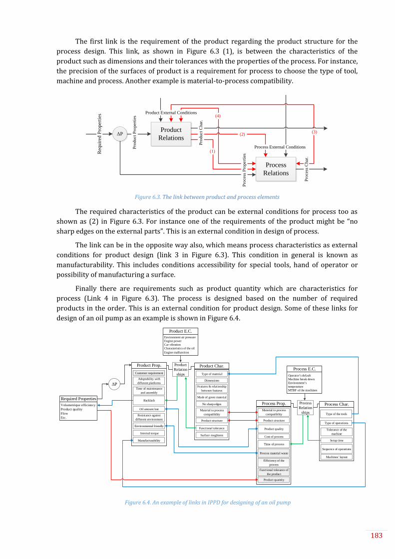
183
The first link is the requirement of the product regarding the product structure for the
process design. This link, as shown in Figure 6.3 (1), is between the characteristics of the
product such as dimensions and their tolerances with the properties of the process. For instance,
the precision of the surfaces of product is a requirement for process to choose the type of tool,
machine and process. Another example is material-to-process compatibility.
ΔPProduct
Relations
Process
Relations
Req
uir
ed P
roper
ties
Pro
du
ct P
rop
erti
es
Pro
cess
Ch
ar.
Product External Conditions
Pro
cess
Pro
per
ties
Process External Conditions
Pro
du
ct C
har
.
(1)
(2)(3)
(4)
Figure 6.3. The link between product and process elements
The required characteristics of the product can be external conditions for process too as
shown as (2) in Figure 6.3. For instance one of the requirements of the product might be “no
sharp edges on the external parts”. This is an external condition in design of process.
The link can be in the opposite way also, which means process characteristics as external
conditions for product design (link 3 in Figure 6.3). This condition in general is known as
manufacturability. This includes conditions accessibility for special tools, hand of operator or
possibility of manufacturing a surface.
Finally there are requirements such as product quantity which are characteristics for
process (Link 4 in Figure 6.3). The process is designed based on the number of required
products in the order. This is an external condition for product design. Some of these links for
design of an oil pump as an example is shown in Figure 6.4.
Customer requirement
Resistance against
different environment
Adoptability with
different platforms
Time of maintenance
and assembly
Oil amount lost
Backlash
Environmental friendly
Manufacturability
Internal torque
Product Prop. Product Char.
Material to process
compatibility
No sharp edges
Product structure
Dimensions
Features & relationship
between features
Made of green material
Type of material
Surface roughness
Functional tolerance
Product
Relation
ships
Process Prop. Process Char.Process
Relation
ships
Efficiency of the
process
Process material waste
Functional tolerance of
the product
Product quality
Cost of process
Time of process
Material to process
compatibility
Product quantity
Product structureType of operations
Machines� layout
Type of the tools
Tolerance of the
machine
Setup time
Sequence of operations
Environment air pressure
Engine power
Car vibration
Characteristics of the oil
Engine malfunction
Product E.C.
Operator�s default
Machine break down
Environment�s
temperature
MTBF of the machines
Process E.C.
ΔP
Volumetrique efficiency
Product quality
Flow
Etc.
Required Properties
Figure 6.4. An example of links in IPPD for designing of an oil pump

184
So, there are different types of links between the elements of product and process in
concurrent designing. All these links have to be considered in the process of design. These links
generate complexity in the design. In addition, there is always certain level of uncertainty in the
links and the elements itself. Uncertainty increases complexity.
So, in order to manage complexity in IPPD regarding CPM, the following requirements
need to be satisfied:
Identifying the required properties (RPj)
Identifying the required characteristics of the product to satisfy RPj
Identifying the relationship between characteristics and properties of product
Formalising the model of product
Identifying the characteristics of the process to build the product
Identifying the relationship between characteristics and properties of process
Identifying the external conditions
Identifying the link between the elements of product with the elements of process
Formalising the model of process
The first four requirements can be achieved by the proposed model of chapter 3. The other
requirements are the focus of this chapter. To be noted, there is no specific order in satisfying
these requirements. Instead, many of the steps should be done simultaneously. For instance, the
eighth requirement can be done while identifying the characteristics of the product.
The following section proposes an approach to help to reduce design complexity by concurrent
modelling. In each level of the design, the approach guides the designer through these
relationships, and therefore the designer can make decisions step by step. After formalising the
process model, a decision making process will be done in each level of decomposition to achieve
the best model for product and process. The resulting model can be used to design, analyse
and/or optimise the system (both product and process).
6.4. The proposed approach for concurrent modelling
Regarding the global objective which is to increase value, in product modelling approach,
the performance aspect has been focused to increase the quality. In in this section, the process
aspect is focused. In process aspect, the goal is to minimise “cost”. While studying the process
alone, productivity of the process should be taken into account too. As mentioned earlier, the
same framework is used for modelling approach in concurrent designing. In product domain,
performance was the output. In process domain, PC and PP are the main outputs. So, the
objective in process modelling is to maximise productivity while minimising cost. Therefore, in
CPM ontology, these objectives are the required properties (RPj). Thus, PC and PP are as-is-
properties (Pj) for process model.
For modelling of product and process in a concurrent designing environment, other than a
common framework, a similar approach is necessary. The objective of the approach (as also in
product) is to help the designer in decision making in the design process. So, the approach
should be able to decompose a system level by level based on the requirements to guide the
designer through the process of design. In addition to the requirements of this approach as
discussed in product model, process requirements should be also considered.

185
Thus, in this section, the process requirements are taken into account in each level of
modelling. Therefore, in addition to the functional and structural domains, process domain is
added to the approach. Figure 6.5 is a general demonstration of the approach with these three
domains and four levels of decomposition. The number of levels depends on the complexity of
the system (both product and process) and the objective of the designer. The approach also
includes two domains of CPM for product and process that are not shown in Figure 6.5. Product
model is as described in chapter 3. Due to the size of the process model, it is shown separately.
Level 1 Level 2 Level 3 Level nF
un
ctio
nS
truct
ure
Pro
cess
Detail designF1
S1
P1
F2
S2
P2
F3
S3
P3
Sn
Pn
DecompositionM
app
ing
Figure 6.5. Integrated product/process modelling domains: Function, Structure and Process
In each section of this figure, a model of system is created. In functional domain, Fn are the
functional models of product in different levels of decomposition. In structure domain, Sn are the
structural models of product to satisfy Fn. These two domains existed in the product modelling
approach. The third domain is process domain which includes models of Pn that are required to
provide Sn.
6.4.1. Determination of process model
In product modelling approach, we proposed EFM for modelling the behaviour of the
system and to assure the transition from function to structure. Here, this transition is assured by
adding process requirements. A similar tool should be used here for modelling the process of
manufacturing. As described earlier, MF/IF is the proposition of this thesis for modelling a
process to be integrated in the IPPM. According to MF/IF a process can be divided into four
elements:
Operate (O): any activity that adds value to the product including manufacturing,
assembly etc.
Transport (T): Moving material, parts, components or product from one place to another
in the value chain from suppliers to customers. It includes internal and external
transports.
Control (C): It insures the functioning of elements as well as the quality of the product.
Storage (S): Anywhere in the supply chain that the material, parts or product is stored or
is waited for the operation is a Storage.
Due to the name of elements, we denote it as “OTCS”. A general representation of this
model in the highest level is illustrated as Figure 6.6.

186
Figure 6.6. A general representation of the OTCS model
According to material flow, input value generally includes resources such as materials,
parts, operators etc. The output value is normally the final product that is delivered to the
customer. Regarding the information flow, the internal flow is the interest of this approach.
However, while modelling and designing a process, information such as management decisions,
suppliers’ information, customers’ requests etc. need to be taken into account also.
In the next level of decomposition, each of these elements can be divided into different
types. Figure 6.7 shows a classification for different types of operate, transport, control and
storage. This classification can also be used for identification of the elements. So, the number and
existence of these elements depend on the case, but the type is placed in one of these categories.
Using the same terminology is important in inter-disciplinarily communications, programming,
and decision making.
Figure 6.7. Different activities of each element
So, by using the model of OTCS in the framework of CPM, and combining the process
requirements to the product approach’s decision making process, the integrated
product/process modelling (IPPM) approach is presented here.
Figure 6.8 shows the domains of the approach including four levels of decomposition
while it shows the product approach as presented in chapter 3. The product approach which is
based on EFM is recalled by illustration of Figure 6.8.
Operate Transport
Control
Transport
Input value Output valueStorage Storage
Process
Operate Manufacturing
Assembly
Transport
Arrival
Internal
Departure
Control
Monitoring
Confirmity
Maintenance
Storage
Raw material
Buffer
Final product

187
Figure 6.8. The product modelling approach in IPPM
In IPPD, the process modelling has a parallel approach with product modelling. In each
level of the approach, the process requirements are added into consideration. So, the approach
creates a model of product by considering the process cost. In addition, a model of process will
be created in CPM framework. This model is used to calculate the total cost and productivity.
In the process domain, the model of process is determined in each level of decomposition
as denoted Pn. P1 is the manufacturing system required to manufacture the required system in
S1. P2 is the decomposition of P1 based on the requirements of S2 and so on. From P3 to Pn
there might be several levels of model decomposition. This decomposition is done to identify the
process characteristics and be able to calculate the process cost and process productivity. This
process is illustrated as a simplified model in Figure 6.9.
Figure 6.9. The process modelling approach in IPPM
So, first it will be explained how each model in process domain is created by using OTCS.
Then, in the mapping axis, it will be shown how these models can be used to determine the
process model in CPM to calculate the total process cost and process productivity. Finally, the
models and the result of CPM will be used to help the designer in decision making process in
each step of the approach.
6.4.2. Mapping: OTCS - CPM
The first level of process model (P1) is created based on S1. This model is shown in Figure
6.10. The inputs of this model are resources including raw material, and the output is the final
product delivered to the client. So, the system as a black box is the required manufacturing
system to produce and deliver the final product.
Level 1 Level 2 Level 3 Level n
Fu
nct
ion
Str
uct
ure
Pro
cess
Detail designF1
S1
P1
F2
S2
P2
F3
S3
P3
Sn
Pn
Level 1 Level 2 Level 3 Level n
Funct
ion
Str
uct
ure
Pro
cess
TI
Detail designF1
S1
P1
F2
S2
P2
F3
S3
P3
Sn
Pn

188
Figure 6.10. First level of process model (P1)
Similar to product modelling approach, in process modelling, in each level of
decomposition, the process model in CPM is determined. Two parameters of PC and PP are the
as-is-properties (Pj). To have coherence with product model, we can consider them as two
parameters of Process Value (PV). So, we can assume the following formula.
𝑃𝑉 = 𝑓(𝑃𝐶, 𝑃𝑃) (6.1)
This is not a precise formula, and it is only used to have an index for process value. Eq. 6.1
can be shown as {PV=PP/PC} to indicate that increasing value can be achieved by minimising PC
and maximising PP. However, PC and PP are dependant and therefore we cannot have two
separated CPM models. Figure 6.11 shows the first level of process model in CPM.
Figure 6.11. Determination of process model in the first level
The second level starts with product model in functional domain. After the determination
of the models F2 and S2, the model P2 is created accordingly. To create P2, the model of OTCS as
shown in Figure 6.6 is used. However, the model is created based on the product model which is
decomposed based on CTOC elements. So, as a general representation, the process model will be
like Figure 6.12.
Delivered Oil pump
Operate:
Transmit system
Assemble
final product
Deliver oil
pump
Operate:
Conversion systemS
Operate:
Operation system
OT2 OC2
OT3 OC3
OT4 OC4
OC1TCTT
OT1
SC
Operate:
Control systemOT5 OC5
Resources
Resources
Resources
Resources
Figure 6.12. Second level of process level (P2)
Resources Manufacturing
System
Delivered
final
productPCPP
PV
PC
PP
R1
Resources Manufacturing
System
Delivered
final
productPCPP

189
In order to provide each element of CTOC, a process is required. So, in Figure 6.12 there
are four elements of “operate” to provide each element of CTOC. In addition, another operate
element is required to assemble these components or group of components. Furthermore,
storage and transport exist in different forms. There might be storage for the final product
before delivering to the client and the product should be delivered to the client. In this level or
any other level of OTCS, the number of elements, their order and their existence are different
from case to case.
The determination of the important parameters in this level is based on OTCS
categorisation as Figure 6.7. As always, the equation between the parameters should be
identified. In this level, the process cost (PC) is divided into the cost of each OTCS element. So the
first general equation is as Eq. 6.2.
𝑃𝐶 = 𝑂𝐶 + 𝑇𝐶 + 𝐶𝐶 + 𝑆𝐶 (6.2)
Where;
OC: Operate cost
TC: Transport cost
CC: Control cost
SC: Storage cost
Other than the cost, productivity (PP) in the process is crucial. PP is considered as the
second Pj. Therefore, it should be calculated as well. Productivity is the number of final products
in a period of time. So, we define productivity as a function of activities’ times.
𝑃𝑃 =
𝑁𝑃
𝑂𝑇 + 𝑇𝑇 + 𝐶𝑇
(6.3)
Where;
NP: Number of final products
OT: Operate time
TT: Transport time
CT: Control time
The storage time is not one of the parameters since the cost of storage in this case is
directly related to the time of storage. However, depending on the case and calculation method,
it can be added. A model of process in the second level is shown in Figure 6.13.
Figure 6.13. Determination of process model in the second level
PV
PC
PP
R1
OC
TC
CC
R2
SC
R3
OT
TT
CT
NP

190
In the same way, P3 is determined based F3 and S3. This approach continues until all the
required parts for the product is determined and the process of “providing” parts is
known/decided. Providing includes manufacturing or buying. In level 3 and the following levels,
the equations are depend on the MF/IF. Here is a list of general equation based on the
classification of Figure 6.7. Table 6.1 is the list of parameters that are used in these equations.
𝑆𝐶 = 𝑆𝐶𝑀 + 𝑆𝐶𝐵 + 𝑆𝐶𝑃 (6.4)
𝑇𝐶 = 𝑇𝐶𝐴 + 𝑇𝐶𝐼 + 𝑇𝐶𝐷 (6.5)
𝐶𝐶 = 𝐶𝐶𝑀𝑜 + 𝐶𝐶𝐶𝑜 + 𝐶𝐶𝑀𝑎 (6.6)
𝑂𝐶 = 𝑂𝐶𝑀 +𝑂𝐶𝐴 + 𝑂𝐶𝑆 (6.7)
𝑂𝑇 = 𝑂𝑇𝑀 + 𝑂𝑇𝐴 + 𝑂𝑇𝑊 (6.8)
𝑇𝑇 = 𝑇𝑇𝐴 + 𝑇𝑇𝐼 + 𝑇𝑇𝐷 + 𝑇𝑇𝑊 (6.9)
𝐶𝑇 = max (𝐶𝑇𝑀𝑜, 𝐶𝑇𝐶𝑜, 𝐶𝑇𝑀𝑎) (6.10)
Table 6.1. The parameters in the equations 6.4 – 6.10
SCM Storage Cost of raw Material OCA Operate Cost – Assembly SCB Storage Cost of Buffers OTM Operate Time – Manufacturing SCP Storage Cost of final Product OTA Operate Time – Assembly TCA Transportation Cost - material Arrival OTW Operate Time – Waste TCI Transportation Cost – Intermediary TTA Transport Time – material Arrival TCD Transportation Cost - product Delivery TTI Transport Time – Intermediary CCMo Control Cost – Monitoring TTD Transport Time – product Delivery CCCo Control Cost – Conformity TTW Transport Time – Waste CCMa Control Cost – Maintenance CTMo Control Time – Monitoring OCS Operate Cost – Scrap CTCo Control Time – Control OCM Operate Cost – Manufacturing CTMa Control Time - Maintenance
The model of process in the third level is illustrated in Figure 6.14. The determination of
the models in CPM for each element is illustrated in appendix B.
ConformityMonitoring Maintenance
Delivered
final productMaterial
Trasport raw
material
T
Manufacturing
O
OCMOTMTCATTA
SCB SCP
Assembly
O
OCAOTA
To assembly
T
TCITTI
Transport
Final product
T
TCDTTD
SCM SCB TTWOCS
CCMoCTMo CCCoCTCo CCMaCTMa
C C C
Figure 6.14. Third level of process level (P3)
So, each element of OTCS can be decomposed based on the type of that element. The
number of decomposition levels for product and process is not necessarily the same. The
product might need more detail analysis while the process cost and time can be easily calculated.
In another case, the process might need more decomposition to analyse the cost and time of
each activity in a very detailed level. The IPPM approach is shown in Figure 6.15.

191
Figure 6.15. IPPM approach to create the model of product and process
To sum up, in each level of decomposition, based on the functional model and structural
model of that level, the process model is determined. One of the most important characteristics
in detail design of product is tolerance. The tolerance allowance of important entities is a
requirement for the process design in detail level. Important entities are those that are identified
in the energy flow because these entities are directly related to the functioning of the system.
The tighter the tolerance, better quality of a product is achieved. On the other side, the lower
tolerance allowance of the system, higher cost of process will be. So, here there is a trade-off
between quality and cost. Tolerancing is one of the means to connect product model to process
model.
Based on the required/chosen level of quality, the tolerance intervals (TI) are determined.
TI is a requirement in process design which can be related to various issues such as machine
precision. TI is the result of process capability as shown in Eq. 6.11.
𝐶𝑝 =
𝑈𝑆𝐿 − 𝐿𝑆𝐿
6𝜎=𝑈𝑇𝐿 − 𝐿𝑇𝐿
6𝜎 (6.11)
Where;
Upper Specification Limit (USL) = Upper Tolerance Limit (UTL)
Lower Specification Limit (LSL) = Lower Tolerance Limit (LTL)
So, the capability of every process should be considered. There might be several processes
for one entity. In this case, TI of that entity becomes the specification limit for the capability of
related processes together. If Cp of process is known, the cost of scrap (OCS) can be calculated
using Eq. 6.12.
𝑂𝐶𝑆 = 𝑁𝑃. 𝑈𝑆𝐶 × (𝐹𝑅. 2 × (1 −1
√2𝜋𝑒−
𝐶𝑝2
2 ) + 𝛼. (1 − 𝐹𝑅) + 𝛽. 𝐹𝑅) (6.12) 5
Where;
NP: Number of Products
USC: Unit Scrap Cost
FR: Failure Rate
α: Error Type-I
β: Error Type-II
Cp: Process Capability
5 This formula is subjected to the hypothesis that manufacturing defaults are independent normal
distributed random variables.
Level 1 Level 2 Level 3 Level n
Fu
nct
ion
Str
uct
ure
Pro
cess
TI
Detail designF1
S1
P1
F2
S2
P2
F3
S3
P3
Sn
Pn

192
Error Type-I is the incorrect rejection of a true hypothesis. In manufacturing process, it
means considering a product as default when it is not actually. Error Type-II is failure to reject a
false hypothesis. In manufacturing process, it happens when after inspection; a default is
considered as a good product.
OCS is one of the parameters in the lowest level of process decomposition to calculate cost.
This parameter along with other parameters like operation time is used to calculate total
process cost (PC). This is a bottom-up approach for cost calculation as shown in Figure 6.16. In
other words, by using the relationships between the elements of P4, P3, P2 and P1, different
types of cost can be calculated and eventually the total cost will be achieved.
Level 1 Level 2 Level 3 Level 4
Fu
nct
ion
Str
uct
ure
Pro
cess
Cost/
Productivity
Calculations
TI
Detail designF1
S1
P1
F2
S2
P2
F3
S3
P3
S4
P4
Figure 6.16. The bottom-up approach for calculating process cost and time
Operations’ time can also be used to calculate PP in a similar bottom-up approach.
Measuring time of tasks in the most decomposed level is more manageable. Using the MF/IF and
the proposed decomposition approach, the designer can know what to look for in each level of
decomposition. After measuring the time and process capability, the total time of each element
and entity of the manufacturing system can be calculated and eventually PP is achieved. The next
sub-section describes how it can help the designer in decision making.
6.4.3. Decision making in IPPM
The decision making is in every part of the approach. As mentioned earlier, the decisions
for structural models are based on the functional requirements. Moreover, based on the
structural model, the decisions related to process model are made. In other words, the structure
model indicates what the product (or any part of the product) needs to satisfy the function, and
in the process model it is decided how to “provide” that. Providing includes producing, partly
producing or completely sub-contracting.
After calculation of process cost, the decisions for structure are being taken according to
the cost of process. This decision making is done in all levels of decomposition. In level 1, the
cost of solution is compared with the required function. For instance, if both product A and
product B can be used to satisfy function X with the same level of quality, the cheaper product is
chosen. Likewise, if the cost of both products is the same, the product that creates higher quality
and better function is chosen. Figure 6.17 shows that process model effects on structural model
of each level in making decisions.
To be noted, if any decision is made to modify the model, it must be based on the
functional model of that level and the models in lower levels should be modified accordingly
(downstream effect).

193
Figure 6.17. Decision making for structural model based on the process model
The decision making between structural model and process model includes a two-way
verification in each level of decomposition as illustrated in Figure 6.18. One of the most
important verification in detail design is tolerance analysis. As indicated, the tolerance
requirements are used to link product model to the process model.
Level 1 Level 2 Level 3 Level 4
Fu
nct
ion
Str
uct
ure
Pro
cess
Cost/
Productivity
Calculations
Detail designF1
S1
P1
F2
S2
P2
F3
S3
P3
S4
P4
Figure 6.18. Two-way verification process in IPPM approach
Another analysis to use in decision making process is risk analysis. A common tool for risk
analysis is Failure Mode, Effects Analysis (FMEA). FMEA is a systematic technique for failure
analysis and it mitigates risk analysis in systems, processes, design or services (H.-C. Liu et al.,
2013). It identifies the potential failure to enhance the reliability of the complex systems. By
FMEA and MF/IF one can identify the importance of the entities in the process. Entities in the
lowest level are the operations. So, the importance of an operation can be interpreted as how
bad the consequences would be in case of malfunction. So, the risk of malfunction needs to be
measured. By analysing the risk in the lowest level, the accumulating risks in the upstream levels
can be calculated or estimated. This analysis and the more detail of calculations are explained
further on the case study.
6.5. Case study
In order to have a better vision toward the proposed approach for concurrent modelling,
the same case as chapter 4 (oil pump) is used. In concurrent modelling there are three domains
of functional, structural and process, plus two models in CPM. For functional and structural
domains, the models of chapter 4 will be used. In process domain, the as-is-properties are cost
and productivity of the manufacturing process of the pump. The data for manufacturing oil
pump provided by Pierburg® is used in this case study.
In this process, only two components of CPHF and CRPH are produced in the factory. Other
components are subcontracted and they only arrive for assembly. There is one station of
Level 1 Level 2 Level 3 Level 4
Fu
nct
ion
Str
uct
ure
Pro
cess
Cost/
Productivity
Calculations
TI
Detail design
F1
S1
P1
F2
S2
P2
F3
S3
P3
S4
P4
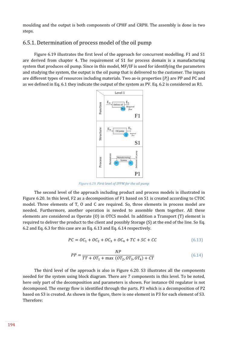
194
moulding and the output is both components of CPHF and CRPH. The assembly is done in two
steps.
6.5.1. Determination of process model of the oil pump
Figure 6.19 illustrates the first level of the approach for concurrent modelling. F1 and S1
are derived from chapter 4. The requirement of S1 for process domain is a manufacturing
system that produces oil pump. Since in this model, MF/IF is used for identifying the parameters
and studying the system, the output is the oil pump that is delivered to the customer. The inputs
are different types of resources including materials. Two as-is properties (Pj) are PP and PC and
as we defined in Eq. 6.1 they indicate the output of the system as PV. Eq. 6.2 is considered as R1.
Figure 6.19. First level of IPPM for the oil pump
The second level of the approach including product and process models is illustrated in
Figure 6.20. In this level, F2 as a decomposition of F1 based on S1 is created according to CTOC
model. Three elements of T, O and C are required. So, three elements in process model are
needed. Furthermore, another operation is needed to assemble them together. All these
elements are considered as Operate (O) in OTCS model. In addition a Transport (T) element is
required to deliver the product to the client and possibly Storage (S) at the end of the line. So Eq.
6.2 and Eq. 6.3 for this case are as Eq. 6.13 and Eq. 6.14 respectively.
The third level of the approach is also in Figure 6.20. S3 illustrates all the components
needed for the system using block diagram. There are 7 components in this level. To be noted,
here only part of the decomposition and parameters is shown. For instance Oil regulator is not
decomposed. The energy flow is identified through the parts. P3 which is a decomposition of P2
based on S3 is created. As shown in the figure, there is one element in P3 for each element of S3.
Therefore:
Fu
nct
ion
Stru
ctu
reP
roce
ss
Deliver oilEm Eh
Oil pumpEm
Eh
RQ
Level 1
Required
flow
Required
flowQ
Res
ou
rces
Del
iver
ed O
il p
um
p
Manufacturing
System
PCPP
F1
S1
P1
𝑃𝐶 = 𝑂𝐶1 + 𝑂𝐶2 +𝑂𝐶3 +𝑂𝐶4 + 𝑇𝐶 + 𝑆𝐶 + 𝐶𝐶 (6.13)
𝑃𝑃 =
𝑁𝑃
𝑇𝑇 + 𝑂𝑇1 +max (𝑂𝑇2, 𝑂𝑇3, 𝑂𝑇4) + 𝐶𝑇 (6.14)

195
𝑂𝐶2 = 𝑂𝐶21 + 𝑂𝐶22 + 𝑂𝐶23 + 𝑂𝐶24 + 𝑂𝐶25 (6.15)
𝑂𝐶3 = 𝑂𝐶31 +𝑂𝐶32 (6.16)
So, the model of process in CPM regarding the identified elements in P1, P2 and P3 is
illustrated in Figure 6.20. This model includes the first and second level parameters and part of
the third level.
Figure 6.20. Second level of IPPM for the oil pump
Figure 6.21. Part of process model of the pump in CPM
Fu
nct
ion
Stru
ctu
reP
roce
ss
Transmit
mechanical
energy
Ø
Generate
hydraulic
energy
Control
Ee EmEm
Eh
R
Generate
oil flow
Deliver oilEm Eh
Oil pumpEm
Eh
RQ
Level 1 Level 2 Level 3
C T O
C
Sprocket+Shaft
+2 pinions
Car
engineØ
2 Pinions +
Casing
Oil
regulator
Hydraulic
hose
Chain
C T OEm Em Em Eh
C
Generate
oil flow
Pump casing
Screws
ibd
Oil pump
Characteristics:
LC, DC, Dr, Db
CPHF
Eh
Characteristics:
Ds, Ls
Big shaftSprocket
Em
Em
Characteristics:
m, Z, H, lp, lh, lb,
LG, DG, Ds
Pinion 1
Em
Oil regulatorEh
Eh
Characteristics:
Ds, Ls
Small shaft
CRPH
Characteristics:
m, Z, H, lp, lh, lb,
LG, DG, Ds
Pinion 2
Em
Eh Eh
VQlMF
Required
flow
Required
flowQ
Eh
Res
ourc
es
Del
iver
ed O
il p
um
p
Manufacturing
SystemPCPR
Del
iver
ed O
il p
um
p
Assemble
final product
Deliver oil
pump
S
Operate:
Sprocket
Operate:
Big shaft
Operate:
Pinions
Operate:
Small shaft
Operate:
CPHF
Operate:
CRPH
Operate:
Regulator
OC21
OC22
OC23
OC24
OC31
OC32
F1
S1
P1
F2
S2
P3
S3
ηvηhm
OC2S
Del
iver
ed O
il p
um
p
Operate:
Trasmit
system
Assemble
final product
Deliver oil
pumpOperate:
Conversion
system
S
Operate:
regulator
OT2 OC2
OT3 OC3
OT4 OC4
OC1TCTT
OT1
P2
SC
Control
CT CC
OC3S
PV
PC
PP
R1
OC1
TC
CC
R2
SC
OC22
OC23
R7
OC21
R3
OT3
TT
CT
NP
OC2
OC3
OC4
OT1
OT2
OT4
OC32
OC2S
OC31
OC2S
R7

196
To calculate time and cost, further decomposition is required and certain decisions should
be made. Figure 6.22 is a schema of the production process of the oil pump from material and
components supply until delivering the final product to the customer. As indicated earlier, a
component can be fully manufactured, partly manufactured or cub-contracted. Two components
of CPHF and CRPH are moulded and machined in the process. However, other components are
prepared and arrive to the assembly line.
Figure 6.22. Process of production of the oil pump
In OTCS the material flow is studied individually for each component to identify the
important parameters of the process. These parameters are used in information flow to calculate
the cost and time of the process assigned to this component. Therefore, regarding the process in
Figure 6.22, the material flow of each component along with the important parameters is shown
in Figure 6.23.
Figure 6.23. Material flow for each component of the oil pump
TAluminum
ArrivalRaw
alu
min
um
O
Molding 1
TMolding to
Machining
O
Machining
TMachining
to Assembly
O
Assembly 1
O
Assembly 2
T Final
product
delivery
Del
iver
ed o
il p
um
p
TMolding to
Machining
O
Machining
TMachining
to Assembly
Co
mp
on
ents
Joints, Cylinder, Spring
TComponent
Arrival
Sprocket, Big shaft, Small shaft, Pinions
CPHF
CRPH
Component
ArrivalAssembly 1 Assembly 2
Final
product
deliveryTCA1TTA1
SC1OTA11OCA11 OTA21OCA21
SC
TCTT
Sprocket
Component
ArrivalAssembly 1 Assembly 2
Final
product
deliveryTCA2TTA2
SC2OTA12OCA12 OTA22OCA22
SC
TCTT
Big shaft
Component
ArrivalAssembly 1 Assembly 2
Final
product
deliveryTCA3TTA3
SC3OTA13OCA13 OTA23OCA23
SC
TCTT
Pinions
Component
ArrivalAssembly 1 Assembly 2
Final
product
deliveryTCA4TTA4
SC4OTA14OCA14 OTA24OCA24
SC
TCTT
Small shaft
Assembly 1 Assembly 2
Final
product
deliverySC7OTA15OCA15 OTA25OCA25
SC
TCTT
Aluminum
Arrival
TTA5
Molding 1Molding to
MachiningMachining
Machining
to Assembly
CPHF
TCI2TTI2OTM12OCM12TCI1TTI1OCM11OCM11TCA5SC6SC5
Assembly 1 Assembly 2
Final
product
deliverySC10OTA16OCA16 OTA26OCA26
SC
TCTT
Aluminum
Arrival
TTA6
Molding 1Molding to
MachiningMachining
Machining
to Assembly
CRPH
TCI2TTI2OTM22OCM22TCI3TTI3OCM21OCM21TCA6SC9SC8

197
The equations and the model of process in CPM until this level of decomposition can be
obtained in the same way as before. Because of the simplicity of the equations, these equations
are not shown here.
Other than different types of operation costs that mentioned in P3, Scrap cost (OCS) needs
to be calculated too. To do that some of the elements in this level, need to be decomposed
further. CPHF was taken as the most important component of the product in chapter 4. The main
operation for this part is machining. So, we decided to decompose this element further.
6.5.2. Detail process model of the oil pump
The part CPHF is shown in Figure 6.24 and its machining process is illustrated in Figure
6.25. The input is the part after molding and transporting to the machining station. Each sub-
operation of the process is an “Operate”. The motions between the operations/machines are part
of the element of “Transport” as shown by “T” in the figure.
Figure 6.24. CPHF and its important entities
Positioning
of the piece
Surface
roughing:
PL100
T
Surface
roughing:
PL101
TFinishing:
CY110T
Roughing:
CY108 &
CY109
TCPHF
Chamfering:
CY108 &
CY109
T
Chamfering:
CY100
Chamfering:
CY101
Finish
boring:
CY101
T
Roughing:
CY102 &
CY103
T
Roughing:
CY111
T
Finishing:
CY108 &
CY109
T
Finishing:
CY102
&CY103
TFinishing:
CY111T
Surface
finishing:
PL100
T
Surface
finishing:
PL101
T T
CpTi Ti Cp Ti Cp Ti Cp Ti
Cp Ti Cp Ti Cp Ti Cp Ti Cp Ti
Cp Ti Cp Ti Cp Ti Cp Ti Cp Ti Cp TiTi
Machined
CPHF
Figure 6.25. Machining process for CPHF
In this level, two most important parameters of each operate box are Time (Ti), and
Process capability (Cp). Using the formula in Eq. 6.12, OCS can be calculated based on NP, USC,
FR, α and β.
Time of each operation can be used for calculation of both cost and productivity. The main
part of the product (CPHF) is studied in this level to demonstrate how it can be calculated for all
of the parts that are produced in the factory. Regarding the process as shown in Figure 6.25,
Table 6.2 shows the time associated with each action. Moreover, the cost of production per unit
of hour and other important costs are as followed:

198
Cost of production = 2.083 € per min
Cost of metrology = 2.25 € per min
Cost of recycling = 1 € per piece
Cost of external failure of the product = 110 € per product
Table 6.2. The order and time of operations for CPHF
Operation Manufacturing
time of one piece (min)
Stage time
(min) Operation
Manufacturing time of one piece (min)
Stage time
(min) Setup 240,000
Tool approach 0,030
25711 Mounting the piece 0,120
Finish boring CY101 0,197 Tool approach 0,030
14769 Tool exit 0,030
Surface roughing PL100 0,088 Changing the piece 0,066 6600 Tool exit 0,030 Tool approach 0,030
12159 Changing the piece 0,066 6600 Roughing CY102 & CY 103 0,062 Tool approach 0,030
16616 Tool exit 0,030
Surface roughing PL101 0,106 Changing the piece 0,066 6600 Tool exit 0,030 Tool approach 0,030
10927 Changing the piece 0,066 6600 Roughing CY111 0,049 Tool approach 0,030
13330 Tool exit 0,030
Finishing CY110 0,073 Changing the piece 0,066 6600 Tool exit 0,030 Tool approach 0,030
13391 Changing the piece 0,066 6600 Finishing CY108 & CY 109 0,074 Tool approach 0,030
15424 Tool exit 0,030
Roughing CY108 & CY 109 0,094 Changing the piece 0,066 6600 Tool exit 0,030 Tool approach 0,030
12159 Changing the piece 0,066 6600 Finishing CY102 & CY103 0,062 Tool approach 0,030
9015 Tool exit 0,030
Chamfering CY108 & CY109 0,030 Changing the piece 0,066 6600 Tool exit 0,030 Tool approach 0,030
12159 Changing the piece 0,066 6600 Finishing CY111 0,062 Tool approach 0,030
25084
Tool exit 0,030 Chamfering CY100 in 45° 0,080 Changing the piece 0,066 6600
Tool approach 0,030 Tool approach 0,030 11674 Chamfering CY101 in 45° 0,080 Surface finishing PL100 0,057
Tool approach 0,030 Tool exit 0,030 Changing the piece 0,066 6600 Changing the piece 0,066 6600
Tool approach 0,030 25711
Tool approach 0,030 12869 Finish boring CY101 0,197 Surface finishing PL101 0,069
Tool Approach 0,030 Tool exit 0,030 Changing the piece 0,066 6600 Changing the piece 0,066 6600
Changing the tool 2,5 550
Since, in our approach, we are looking for the important characteristics and their cost of
production, the cost of each entity is obtained based on Table 6.2. The result is shown in Table
6.3.
Table 6.3. Cost of entities derived from the cost of operations
Surface Operations Time of 100000
operations (min) Cost of surface
manufacturing (€)
PL100 Surface roughing
39644 82578 Surface finishing
PL101 Surface roughing
42685 88913 Surface finishing
CY100 Chamfering 45°
48154 100304 Finish boring
CY101 Chamfering 45°
48154 100304 Finish boring
CY102,CY103 Roughing
37520 78154 Finishing
CY108,CY109 Roughing
57632 120047 Chamfering 45° Finishing
CY110 Finishing 19930 41514
CY111 Roughing
36288 75588 Finishing

199
After identifying the cost of entities, the data can be combined with TAFT analysis that is
illustrated in chapter 4 (Table 4.3) as shown in Table 6.4. In this way, the cost of “FTE” is
obtained. To be noted, the total cost for Table 6.3 and 6.4 stays equal (6.87 €/part).
Table 6.4. Cost of ETFs
The scrap cost is related to process capability. The process of machining CPHF includes
several operations. So, the combination of operations capabilities gives the process capability.
There is no general formula to calculate Cp of the machining process based on the Cp of each
operation. Normally in this case the Cp of the process is taken into account. Here, as an example
we consider the Cp of the process as the minimum of all Cps.
𝐶𝑝 = min (𝐶𝑝𝑖) (6.17)
The other type of parameter is operation time. This parameter can be measured for each
operation or for the whole process. This depends on the objective of the designer. If the designer
aims at optimising a specific operation, or designing operations, the former measurement is
used. If all the operations are done on one single machine for instance, the process time of the
machine is considered.
Another cost that should be calculated is the cost of control (CC). As shown in Eq. 6.6, it
includes monitoring, conformity and maintenance. The cost of each of these parameters can be
calculated based on the cost of each control and its frequency as shown in Eq. 6.18, Eq. 6.19 and
Eq. 6.20.
No. Identification-Action Liaisons - Surfaces Cost
FTE on what Complement Surf.1 Surf.2 Surf. 3 Batch 1 part
1 Positioning CRPH Axially PL100 FI10x € 27,526 € 0.28
2 Prevent the
leakage CRPH Flux PL100 FI10x € 27,526 € 0.28
3 Positioning CRPH With pressure PL100 FI10x € 27,526 € 0.28 7 Positioning Engine casing Axially PL101 CY109 CY108 € 74,468 € 0.74 8 Positioning Engine casing With pressure PL101
€ 44,456 € 0.44
9 Positioning Fixation to engine Axially CY109 CY108 € 30,012 € 0.30 10 Positioning Fixation to engine Angularly CY109 CY108 € 30,012 € 0.30 11 Passing Fixation to engine Radially CY109 CY108 € 30,012 € 0.30 12 Positioning Oil exit Axially CY110
€ 13,838 € 0.14
13 Positioning Oil exit Radially CY110
€ 13,838 € 0.14 14 Positioning Big axis Axially CY111 CY102 € 38,222 € 0.38 15 Positioning Big axis Radially CY111 CY102 CY112 € 38,222 € 0.38 16 Passing Big axis Radially CY111 CY102 CY112 € 38,222 € 0.38 17 Positioning Little Axis Axially CY103
€ 19,539 € 0.20
18 Passing Little Axis Radially CY103
€ 19,539 € 0.20 19 Positioning Little pinion 1 Axially CY100 CH100 € 33,435 € 0.33 20 Positioning Little pinion 1 Angularly CY100 CH100 € 33,435 € 0.33
21 Passing Little pinion 1 Radially CY100 CH100 PL102 PL103 PL104
€ 33,435 € 0.33
22 Positioning Little pinion 2 Axially CY101 CH101 € 33,435 € 0.33 23 Positioning Little pinion 2 Angularly CY101 CH101 € 33,435 € 0.33
24 Passing Little pinion 2 Radially CY101 CH101 PL102 PL103 PL104
€ 33,435 € 0.33
25 Passing Oil with proper
volume & pressure
PL105 CY110 PL102 PL103 PL104
€ 13,838 € 0.14

200
𝐶𝐶𝑀𝑜 = 𝐶𝑀𝑜 × 𝐹𝑀𝑜 (6.18)
𝐶𝐶𝐶𝑜 = 𝐶𝐶𝑜 × 𝐹𝐶𝑜 (6.19)
𝐶𝐶𝑀𝑎 = 𝐶𝑀𝑎 × 𝑛 (6.20)
In these equations CMo, CCo and CMa are the cost of monitoring, conformity and maintenance
respectively. FMo and FCo are the frequency of monitoring and conformity. Since maintenance is
done on all the parts, number of products (n) is the frequency. n is different from NP that is
introduced earlier. n is the number of produced products including the defaults but NP is the
number of final products that are shipped to the customer.
6.5.3. Risk analysis of the process of the oil pump
Other than cost and productivity, risk analysis is required in this stage to reduce
complexity that is caused by uncertainty. As stated, FMEA is used for risk analysis. In product,
the objective of the flow analysis was to assure the passage of oil as smooth as possible with
enough flow and pressure. According to energy flow analysis, assuring the transmission and
conversion of two flows of mechanical energy and hydraulic energy is the function of the system.
Any issue that causes malfunction should be eliminated or at least reduced.
By FMEA we can identify the possible problems in the process that can cause malfunction
in the product. For this analysis, bottom-up approach is used (similar to cost and productivity
calculations). Now that the lowest level entities of the process are determined, FMEA can be
done on the operation regarding the importance (gravity) and capability of each operation. For
this analysis in detail level, the main part (CPHF) is used. The important entities as shown in
Figure 6.24 and the operations for this part are as Figure 6.25.
As Figure 6.25 illustrates, different operations are done on this part. The list of these
operations along with the capability of each operation is listed in Table 6.4. Using Table 6.3, this
information can be sorted by the entities.
Table 6.5. Operations for CPHF and capability of them
Operation Process
Capability (Cp) Process Capability
Index (Pp) Surface roughing PL100 2 1.5 Surface roughing PL101 2 1.5 Finishing CY110 2 1.66 Roughing CY108 & CY 109 1.6 1.33 Chamfering CY108 & CY109 in 45° 2 1.66 Chamfering CY100 & CY101 in 45° 2 1.66 Finish boring CY100 1.5 1.2 Finish boring CY101 1.5 1.2 Roughing CY102 & CY 103 1.66 1.3 Roughing CY111 1.66 1.4 Finishing CY108 & CY 109 1.66 1.4 Finishing CY102 & CY103 1.3 1.1 Finishing CY111 1.3 1 Surface finishing PL100 1.66 1.33 Surface finishing PL101 1.66 1.33

201
Similarly, using TAFT analysis each entity can be analysed regarding the related action(s).
The result is shown in Table 6.6. In this table, the possible failure mode regarding the action can
be predicted. According to that, gravity is assigned.
Table 6.6. TAFT including FMEA
No. Identification-Action Liaisons
- Surfaces
Risk
ETF on what Complement Failure mode Gravity
1 Positioning CRPH Axially PL100 FI10x
Bad position, Crack 8
2 Positioning 4 x Screw Angularly FI10x Bad angle 0
3 Positioning Engine casing Axially PL101 CY109 CY108
Bad position 5
4 Positioning Engine casing With pressure PL101 Bad position, Not enough pressure 1 5 Positioning Oil exit Axially CY110 Bad position, Not smooth enough 2
6 Positioning Big axis Axially CY111 CY102
Bad position, Crack 10
7 Passing Little Axis Radially CY103 Unable to pass, too large to keep 4
8 Positioning Little pinion 1 Axially CY100 CH100
Bad position, Crack 7
9 Positioning Little pinion 2 Axially CY101 CH101
Bad position, Crack 7
10 Passing Oil With proper volume and
pressure
PL105 CY110 PL102 PL103 PL104
Pad position, Leakage, Too large to have enough pressure
4
The values for gravity can be studied in a top-down approach. These values are assigned to
surfaces related to each action. Then it can be assigned to the related operations as it is shown in
Table 6.7.
Table 6.7. List of important entities and the related operations
Surface Operations Gravity Surface Operations Gravity
PL100 Surface roughing
10
CY102,CY103 Roughing
9 Surface finishing Finishing
PL101 Surface roughing
4
CY108,CY109
Roughing
10 Surface finishing Chamfering 45°
CY100 Chamfering 45°
9 Finishing
Finish boring CY110 Finishing 5
CY101 Chamfering 45°
9
CY111 Roughing
8 Finish boring Finishing
Finally using this data and Table 6.5 the importance (gravity) of each operation regarding
the function of the product can be obtained (Table 6.8). There are different ways for assigning
gravity with it includes several entities. Choosing the right method depends on the policy of the
manufacturer/designer.
6.5.4. Finalising and decision making
When all the effective parameters and their relations are identified, the model of process
in CPM can be determined. Unlike in chapter 4, the model for the oil pump manufacturing
process is not presented here since there are so many parameters and relations and it will not
be interesting for the audience. Instead, a general model of the process (which can be the
process of manufacturing the pump) is presented to give an overview of the model and types of
relations and parameters. Although, this model is different case by case, most of the elements

202
can be used as a reference for modelling various processes. This model is illustrated in Figure
6.26.
Table 6.8. Operations for CPHF with their capability and gravity
Operation Process
Capability (Cp) Process Capability
Index (Pp) Gravity
Surface roughing PL100 2 1.5 2 Surface roughing PL101 2 1.5 1 Finishing CY110 2 1.66 5 Roughing CY108 & CY 109 1.6 1.33 1 Chamfering CY108 & CY109 in 45° 2 1.66 1 Chamfering CY100 & CY101 in 45° 2 1.66 3 Finish boring CY100 1.5 1.2 8 Finish boring CY101 1.5 1.2 8 Roughing CY102 & CY 103 1.66 1.3 3 Roughing CY111 1.66 1.4 2 Finishing CY108 & CY 109 1.66 1.4 3 Finishing CY102 & CY103 1.3 1.1 7 Finishing CY111 1.3 1 7 Surface finishing PL100 1.66 1.33 9 Surface finishing PL101 1.66 1.33 3
When achieving this kind of model, all the sub-processes are decomposed and the effective
parameters are identified until the most detail level. However, sometimes the values of
parameters in higher levels are known. So, the model can be simplified. This simplification is
directly related to the available data and the objective. It is important not to remove an essential
links while simplifying.
By using the equations in the model, the total cost (PC) and productivity (PP) can be
calculated. Using cost and productivity in each level of process model, certain decisions can be
made in structure model of product. For instance, if the cost of manufacturing of pinions is less
than buying them, the decision to change this choice can be made in P3-S3. All these decisions
are based on the chosen level of quality.
As another example, looking at the decision making process in P2-S2, if transferring
mechanical energy using two sprocket is cheaper than sprocket-chain, and the function in F2 is
satisfied with the required performance, the decision in the second level can be made. Finally, an
external-gear oil pump might not be the most efficient choice. This decision can be made in P1-
S1 using the information regarding the cost, productivity and satisfying the required function.
So, decisions can be made based on the level of quality and cost.
6.6. Application: Tolerance optimisation
In the previous chapter, the applications of the approach and the resulting model in
sensitivity analysis and tolerancing have been shown. By using the proposed approach of this
chapter, the factor of cost can be added to the decision making criteria. Therefore, by having
both aspects of cost and quality, the model can be used for optimising the product if the
approach is about modelling an existing product. So, in this section, as a result of the IPPM
approach, it is explained how the approach and result of sensitivity analysis can be used for
optimisation. The case study is used to show the application.
There are several algorithms and methods for tolerance optimisation in literature. (Dong,
1997; Sfantsikopoulos, 1990; Zong & Mao, 2015) are some of the works that are focused on cost
of tolerance to model and optimise the product. (Iannuzzi & Sandgren, 1996; J. Lee, 1992;

203
Prabhaharan, Asokan, Ramesh, & Rajendran, 2004; Sampath & Alagumurthi, 2010) used genetic
algorithm for tolerance optimisation. Our proposition is to use the approach of chapter 3 and 5
to determine the mathematical link between tolerances and value. Then, existing optimisation
algorithm in literature can be easily used to optimise the product.
Figure 6.26. A full process model in CPM as an example
Due to the step-by-step decision making process of the approach, the approach can be
used for improving the product in each level of decomposition. In addition, the result of the
approach is a quantitative model that can be used in an optimisation algorithm to improve
quality and reduce cost. By focusing on the second application, in this section, it is shortly
explained how the result of the analyses (sensitivity analysis and tolerance analysis) can be used
to initiate the optimisation phase.
PV
PC
PP
R1
OC
TC
CCR2
SC
OCM
OCA
R7
TCA
TCIR5
CCMo
CCCoR6
CCMa
SCM
SCB
SCP
R4
OCS
Transport
capacity
Storage
capacity
R3
TCD
OT
TT
CT
OTM
OTAR8
TTA
TTIR9
TTW,
Transport capacity
TTD
CTMo
CTCo
CTMa
R10
NP
R11
R12
R13
R14
R26
R27
R15
R17
R18
R19
R20
R21
SCM1
SCM2
SCM3
SCB1
SCB6
...
TCA1
TCA2
SCI1
SCI4
FMo
...
CMo
R28 FCo
CCo
R29
n
CMo
R16
OCM1
OCM2
OCM3
OCA1
OCA2
OTM1
OTM2
OTM3
OTA1
OTA2
TTA1
TTA2
TTI1
TTI4
Storage
capacityR22
Production
planningR23
Transp. type
R24
R25
Cost of
Rail transp.
Cost of
Road transp.
Cost of
Transp. means
Cp
FR, USC, α, β
Molding spec
Machine
dispersion
R31
R32
Assembly
spec
R33
...
Adjustment
parameters
Storage
resources
Transp.
resources
Machining
resources
R30
TI
Number of
workers
R34
R35
R36
R37
Number of
trucks
Factory
facilities
Subcontractor
availability
OTW

204
As described in tolerance analysis section, a compromise must be made between designers
who want tight tolerances to assure product performance and manufacturers who prefer loose
tolerances to reduce production cost. Before, it was shown how tolerancing can create a link
between performance and cost. In this section, the objective is to minimize the Marketable
Product Total Cost (MPTC), by quantifying the best possible geometrical tolerances (mostly
dimensional tolerances). The objective function can be defined by the concept of “value” as
defined to consider both aspects of cost and quality. So, value can be calculated as the opposite
of MPTC (Etienne et al., 2016).
To evaluate this value, both aspects of product and process should be taken into account.
Thus, from product aspect, the characteristics and constraints mainly from the requirements
and from process aspect, process capability and costs of resources are taken into calculations.
6.6.1. Problem formulation
Regarding the discussed case study, the required function of the oil pump is to deliver oil
with required flow. So, the objective is to maximise the flow by modifying the tolerances while
considering the cost.
The manufacture of the oil pump expects an oil flow of 4.45×10⁻⁴ m3/s in a specific given
condition. The designers know that the efficiency and oil flow of the pump are related to
different backlashes. As detailed in chapter 4, these backlashes are between the gears and the
casing as well as between the gears and shafts. Too small backlashes will result in friction and
too much of them will result in internal flow loss and therefore performance reduction.
Achieving precise backlashes is the result of manufacturing precision to obtain tight tolerances.
Cost of tolerance is different for different parts and it is related to the level of chosen quality. For
instance, gears are made of aluminium so the quality level of IT8 (from Table 5.2) is chosen for it.
Therefore, because of the diameter of 31mm, the tolerance interval is 39µm. The casing (CPHF)
is made of sintered steel. So, the quality level of IT6 is chosen for all the entities shown in Figure
6.27. The impact of tolerance level on the performance is not clear for the designer. Moreover,
this impact on the cost of production should be identified as well.
Figure 6.27. CPHF and some of its tolerances
There are of course different aspects for analysing the parameters that effect on the cost
and quality. To carry out the evaluation of the value of a product configuration, the tolerance
allocation is coupled with the process generation and its evaluation regarding both its costs and
the impacts of it on the product quality. Other aspects of this problem are discussed in (Etienne
et al., 2016).
Ax

205
As illustrated in chapter 4 and section 6.4, by utilising the proposed approach, the link
between the performance and tolerances is created. The second aspect is to evaluate the
manufacturing process cost. As explained in chapter 5, when the manufacturing process is
generated, the ABC method assesses this parameter. In this approach the cost of all resources as
well as all the parameters need to be known. (not necessarily the exact value, but at least
relatively). When both quality measures and cost assessment are available the evaluation of the
relevance of one tolerance allocation can be done. The quality weighted cost of both the product
and its manufacturing process is available and can be compared with other solutions. In order to
find the product configuration having the best quality weighted cost, an optimisation loop is
needed. At each step of this loop new tolerance allocation is generated and its cost is assessed.
6.6.2. Results
By using MCS and the relations in product model (performance) and process model (cost),
the performance is increased based on the optimised tolerances. So, the result of tolerance
analysis of the previous section is used to optimise the product in this aspect.
For calculations, Mathematica® software is used. The inputs are the same as Table 5.1. So,
there are 12 inputs (Characteristics) that will be analysed and optimised, and four external
conditions with fixed values. 10000 iterations of MCS for 4000 values of each characteristic are
considered. The following constraints are taken into the simulation:
3. The condition regarding the backlashes individually:
ℎ𝑏 ≥ 0 & ℎ𝑟 ≥ 0 & ℎ𝑎 ≥ 0 (6. 14)
4. The condition regarding the chain of tolerances:
0 < 𝑒 < min(
𝐷𝑏 − 𝐷𝑠2
,𝐷𝐶 −𝐷𝐺2
) − 𝐶𝑥 (6. 15)
Figure 6.28 illustrates the evolution of the MPTC of the product configuration which in fact
represents the opposite of the value. With 4000 iterations, this value is equal to 8.01666.
Figure 6.28. Evolution of fitness values during the Genetic Algorithm iterations
Some of the results are highlighted in this report. The following set of diagrams
demonstrates the evolution and consequently the optimisation of tolerance allocation.
0 500 1000 1500 2000 2500 3000 3500 4000Total Number of Generations0
200
400
600
800
1000
Fitness
Iterations of the genetic algorithm
Val
ues
of
fitn
ess

206
Figure 6.29 illustrates the evolution of the tolerances regarding two characteristics of DC
and DG. These two parameters have important impacts as analysed in section 5.2. The reason is
that they create the axial backlash which is between the pinions and the casing (denoted as hr).
The optimised values for tolerances of these characteristics are as followed:
𝑇∗(𝐷𝐶) = 0.092, 𝑇∗(𝐷𝐺) = 0.086
Figure 6.29. Evolution of tolerance values for DC and DG during the Genetic Algorithm iterations
The evolution of the values for this backlash is illustrated in Figure 6.30. The values in this
diagram are in fact the combination of values for DC and DG. (ℎ𝑟 = 𝐷𝐶 − 𝐷𝐺).
Figure 6.30. Evolution of values for hr during the Genetic Algorithm iterations
As it is evident in Figure 6.30, the optimal value for radial backlash (hr) is not equal as
zero. Although in order to increase the performance, the backlashes should be minimised, hr=0
or even hr→0 is not the optimal value. This is because very tight tolerance in this case generates
friction when the pinions are rotating in the casing. This friction can be due to the
decentralisation of the shaft during the functioning or different surface stiffness on the tip of
each tooth.
The second pair of parameters is LC and LG. Figure 6.31 shows the result of optimisation
algorithm for the tolerances of these two parameters. The optimal values are:
𝑇∗(𝐿𝐶) = 0.076, 𝑇∗(𝐿𝐺) = 0.072
0 500 1000 1500 2000 2500 3000 3500 4000Total Number of Generations0.00
0.05
0.10
0.15
0.20
Tolerance 4
0 500 1000 1500 2000 2500 3000 3500 4000Total Number of Generations0.00
0.05
0.10
0.15
0.20
Tolerance 5
0 500 1000 1500 2000 2500 3000 3500 4000Total Number of Generations0.00
0.05
0.10
0.15
0.20
Jeu nominal 1
Val
ues
of
tole
ran
ce f
or
DG
Val
ues
of
tole
ran
ce f
or
DC
Val
ues
of
hr
Upper range
Lower range
Best solution

207
Figure 6.31. Evolution of tolerance values for LC and LG during the Genetic Algorithm iterations
Similarly, the optimised value for the backlash related to these parameters which is ha, is
obtained as shown in Figure 6.32.
Figure 6.32. Evolution of values for ha during the Genetic Algorithm iterations
Finally the third pair of parameters that are related to the backlashes is Db and Ds. These
parameters are related to the bearing backlash. The optimal value for the tolerances of these
parameters as illustrated in Figure 6.33 is as followed:
𝑇∗(𝐷𝑏) = 0.013, 𝑇∗(𝐷𝑠) = 0.008
Figure 6.33. Evolution of tolerance values for Db and Ds during the Genetic Algorithm iterations
0 500 1000 1500 2000 2500 3000 3500 4000Total Number of Generations0.00
0.05
0.10
0.15
0.20
Tolerance 6
0 500 1000 1500 2000 2500 3000 3500 4000Total Number of Generations0.00
0.05
0.10
0.15
0.20
Tolerance 7
0 500 1000 1500 2000 2500 3000 3500 4000Total Number of Generations0.00
0.05
0.10
0.15
0.20
Jeu nominal 2
0 500 1000 1500 2000 2500 3000 3500 4000Total Number of Generations0.00
0.05
0.10
0.15
0.20
Tolerance 11
0 500 1000 1500 2000 2500 3000 3500 4000Total Number of Generations0.00
0.05
0.10
0.15
0.20
Tolerance 10
Val
ues
of
tole
ran
ce f
or
LG
Val
ues
of
tole
ran
ce f
or
LC
Val
ues
of
ha
Val
ues
of
tole
ran
ce f
or
Db
Val
ues
of
tole
ran
ce f
or
Ds

208
Likewise, the optimised value for bearing backlash (hb) is obtained as shown in Figure
6.34.
Figure 6.34. Evolution of values for hb during the Genetic Algorithm iterations
6.7. Conclusion
IPPD is a known solution for today’s industry to increase “value”. However, the number of
links that concurrent designing creates between the elements of product and process generates
complexity. Other than difficulty in identifying the links, uncertainty in these links increases
complexity. The proposed approach of this chapter aimed at reducing this type of design
complexity.
The proposed approach was an extension of the product approach of chapter 3. The
approach which is based on the framework of CPM studies the system by material and
information flow (MF/IF). The material flow is used to identify the links between the elements of
the process. Information flow is used to calculate cost, productivity and risk of each part of the
process. So, in a top-down approach, the process is analysed using material flow to create the
model of process in CPM. Then, in a bottom-up approach the model is used to calculate the as-is
properties of the process and analyse the system.
Generally, as-is properties for process of manufacturing are cost and productivity. To
calculate the cost, the system is decomposed enough to be calculated. In the case study for
instance, in the lowest level, cost of production per hour and time of each operation are
measured in the process. By assigning the related entities to the operations, the cost per each
entity is obtained. These entities are the characteristics in product model. Using the TAFT
analysis the related sub-function (action) to each entity is identified. Finally, the combination of
these actions is the function that the product needs to satisfy. Time of operations has also been
used to calculate productivity. For this calculation a similar bottom-up approach as cost
calculation is used.
Another important parameter in the lowest level of decomposition is capability of
operations. This parameter is used to calculate part of cost that is related to scrap cost. Scrap
cost is identified in Control element and can be affected the elements of Operate, Transport or
Storage. This approach is illustrated in Figure 6.35. Capability is also used for risk analysis. As
uncertainty is discussed for product modelling, risk analysis has an important role in process
0 500 1000 1500 2000 2500 3000 3500 4000Total Number of Generations0.00
0.05
0.10
0.15
0.20
Jeu nominal 3
Val
ues
of
hb

209
modelling. In this thesis we did not go into the detail of this topic but it can be integrated in the
approach using various risk analysis methods like FMEA.
Figure 6.35. The bottom-up approach for cost calculation
Figure 6.36 illustrates all the sub-approaches in IPPM approach. In this approach, F1
shows the objective of the model. S1 is a possible system to satisfy F1. P1 is the required process
to produce S1. F2 is the decomposition of F1 based on S1. In the same way, all the models in each
level of decomposition are determined. In each level, determining the models includes set of
decisions to make. After the creation of all models, the calculated cost in process and
requirements of the model in functional domain are used to improve the structural models in
each level.
Level 1 Level 2 Level 3 Level 4
Fu
nct
ion
Str
uct
ure
Pro
cess
Cost/
Productivity
Calculations
TI
Detail design
F1
S1
P1
F2
S2
P2
F3
S3
P3
S4
P4
Decomposition
Decision Making
Cost calculation
Process requirements
Figure 6.36. IPPM approach
So, after the creation of the process model, the designer can verify each level of
decomposition and add cost, productivity and risk into consideration. So, the changes can be
made for product or process models.
This resulting model can be used to analyse the change impact of each characteristic on
the output (cost or productivity). This is possible using the identified links in the approach. For
instance machine dispersion is one of the characteristics in process model. It is related to both
product and process. As the impact of tolerancing discussed, machine dispersion is one of the
important factors in the tolerances of the product. Using product model, the impact of tolerance-
quality is verified and using the process model, the impact of machine dispersion and process
value can be assessed (as shown with red links in Figure 6.36)
Thus, the proposed approach assures the link between characteristics of the process with
its output. In the lowest level of product, related tolerances of each characteristic can be
analysed. Tolerance is related to the capability of the operations. Therefore, with this approach,
cost considerations are added to the tolerancing process as it the result was shown in the last
section. It is shown how the result of the approach can be used later for optimisation. So, in this
section, by using an optimisation algorithm, different combination of the characteristic (or their
tolerances) can be checked to find the best values for having the maximum output (Q in this
case). Then again, because of the quantitative link between the performance and structure that
the approach is created, it is a very good basis for optimisation algorithm. Here, the optimisation
Total process
cost
Cost of ETF
Cost of entity
Cost of operation
Time of operaion

210
was with focusing on tolerancing. So, two links of quality-tolerance and cost-tolerance have been
used to obtain the optimal value for Q.

211
Conclusion, limitations and perspective
The global objective of this thesis was to help the industry in increasing value of their
products. The concept of value has various meaning in different industries and it depends on the
point of view. In product development, we defined value based on two axes of quality and cost.
Quality is related to product design aspect and cost is related to process design aspect. In order
to consider both aspects, Integrated Product/Process Design (IPPD) has been chosen as the
domain of this thesis. The first research question was:
“How concurrent designing can profit industry and how to assess value in this concept?”
In product development, two departments of product design and process design are highly
dependent on each other to deliver a good result. So, IPPD proposes concurrent designing of
product and process. Concurrent designing means considering process criteria such as
manufacturability and cost in product design and considering product requirements in process
design. In the beginning of chapter 2, concurrent designing and its related concepts such as FBD,
DfX and CE have been explained. So, the answer to the first research question has been
discussed in this section.
In product design, there are elements such as product characteristics, behaviour and
required function. These elements are related to each other and identifying their relationships is
the key for a good design. Likewise, in process design, there are elements such as cost that have
to be considered in product development. In an IPPD system, in addition to all these relations,
there are also so many links between the elements of product design and the elements of
process design. All these relationships create complexity in design. So, here was the second
question on:
“What are the sources of complexity in IPPD and how to manage them?
In order to answer the first part of the question, complexity’s definitions and its sources
are reviewed from different points of view. These visions have been presented in 2.4. We
focused on three main visions: Suh’s, ElMaraghy’s and Weber’s. Accordingly, uncertainty is
considered as one of the main sources of complexity along with causes such as coupling or lack
of knowledge.
In order to answer the second part of the question and to manage complexity, design
parameters should be identified, designer’s knowledge toward the designing system should be
increased and uncertainty should be managed. So, an approach or methodology is required that
can be used as a design framework, it has a systematic approach, it can be used for both product
and process design, it creates a coherence between product and process, it reduces complexity
in design, it has the ability to integrated mathematical equations, it is easy to understand and
learn, it is robust and it can integrate other methods. So, we look for the answer of the fourth and
main question:
“How to model an integrated product/process system systematically to increase “value”?”

212
Various design theories and methodologies have been reviewed to find or create the
required approach. Among them, Characteristics-Properties Modelling is chosen as the
framework of the approach to create a quantitative model of a system. Apart from a framework,
a systematic approach is required to help the designer in the design process.
To answer the above question, the four sub-questions need to be answered. The first sub-
question is:
“How to achieve a robust approach to model a manufacturable product to satisfy the
customer needs?”
The most important aspect in product design is to insure that the required function of the
product is satisfied. The structure of the product should be designed based on the required
function. So, the main challenge is to identify the link between function and structure of the
product. Therefore, in our approach, both domains of function and structure in every level of
design had to be taken into account. So, the zigzag approach of Axiomatic Design has been used
in a systematic approach. Based on axiomatic design, in this approach, by zigzagging between
functional and structural domain, both aspects are taken into account.
In this framework, the challenge was to find the link and model the structure of the system
based on the required function. This link is a physical link between different elements of system
with each other and with the output of the system. For identifying this link, energy flow was
used. EFM defines a system based on the flow of energy. CTOC is one of the EFMs that was used
in our proposed approach. CTOC focuses on the minimum requirement of a system to satisfy the
required function. Energy flow determines the link that is among the parameters of the system’s
structure. In addition, by creating the link between input and output of the product, it
determines the link between the function and structure. So, it increases the knowledge of the
designer about the behaviour of the product.
Thus, as it is explained in chapter 3, the model of CTOC is used in a systematic approach
while zigzagging between functional and structural domains. Instead of the classical CPM, an
extended version of CPM was proposed. In this extended version, modelling is done in a top-
down systematic approach with several levels of properties. So, while creating a pathway for the
designer for modelling a product step by step, it reduces design complexity and ambiguity.
The proposed approach includes two axes of mapping and decomposition. The mapping
axis includes functional domain, structural domain and CPM. The second axis decomposes the
system level by level. So, in each level of decomposition, the system is modelled based on the
required function. Then, the structural model is determined according to the functional model.
The important parameters of each model are determined and being transferred to the model in
CPM. In each model, by the information that is obtained by the energy flow, the model and the
physical phenomena, the relationships between the parameters are determined.
This approach helps the designer to identify the modifiable parameters that are effective
on the product performance. Due to its systematic nature, it also helps the designer in decision
making in every step of modelling and design process. By following the approach and its set of
rules, transition from function to structure will be assured and a quantitative model of the
system will be achieved.
In chapter 4, an automobile oil pump was used for demonstration of the implementation
of the approach. After a primary study of the case, enough information has been obtained to use
the approach for the determination of the model. Since the approach is applicable for an existing
product as well as for designing a new product, the procedure was explained as if the product

213
does not exist to give a better overview in both cases. So, the modelling begins with identifying
the required output of the product which is to deliver oil with required flow. The functional
model includes the function to satisfy the required output. The structural model is determined
based on the functional model and energy flow, which in this case is the oil pump. In the second
level and the subsequent levels, CTOC is used to decompose the model, identify the sub-
functions and structure of the system. In the final level of decomposition, where the structure is
known, IBD (or Bond Graph) was used to determine the exact structure of the oil pump.
This model is also the solution for the third research question:
“How to manage design uncertainty?”
As it is described in chapter 5, the approach can be used for uncertainty management in
design. So, after an introduction of the uncertainty in design, it was described what types of
uncertainty in design can be elicited by the proposed approach. Different types of epistemic and
aleatory uncertainties can be determined and managed while going through the proposed
hierarchical approach. It can also be used for mitigation of specific type of epistemic uncertainty.
Therefore, complexity that is due to uncertainty can be managed. The process of uncertainty
elicitation and propagation has been shown by using the industrial case study.
The determination of the model by using the proposed approach is the first phase of the
approach. The second phase is to use the determined model to study the system and improve it.
The second and third parts of Chapter 5 focused on the second phase to answer the fifth
research question:
“How the model can be used to analyse and optimize the system?”
Thanks to the CTOC and CPM, the determined model includes a quantitative relation
between the output(s) of the product with the effective characteristics. So, the result was used to
analyse the impact of each characteristic on the output. This sensitivity analysis included both
local and global sensitivity analyses. In local sensitivity analysis, the impact of each
characteristic, a combination of characteristics and their variations have been studied. In the
global sensitivity analysis, the importance of characteristics and external conditions were
compared. So, the key characteristics were identified.
One of the most important analyses is tolerance analysis. In the third section of chapter 5
the concept of tolerancing has been explained. It has also been shown how the approach and the
determined model can be used for analysing the impact of characteristics’ tolerances as well as a
chain of tolerances on the performance of the product. This aim was achieve by determining the
link between function and functional tolerances.
The answer of the main question (question 4) is still not completed. The second sub-
question is about modelling the process of manufacturing:
“How to achieve a robust approach to model the process based on the product
requirements?”
Our proposition became completed in chapter 6 by proposing a concurrent modelling
approach. In this chapter, an extension of the approach was proposed to take the manufacturing
process parameters into account in product development. Material flow and information flow
(MF/IF) have been used to model the process, to identify the important parameters and the link
between them. However, the process model cannot be achieved without considering the
decisions and requirements in product design aspect due to their dependencies. Therefore, by
aiming at reducing complexity in IPPD, the concurrent modelling has been proposed.

214
The approach adds a new domain as process to the existed functional and structural
domains. Hence, based on the required structure, the process model is determined. To
decompose the process model, OTCS was proposed. In a top-down approach the model of
process in CPM is determined. After that, in a bottom-up approach, the model is used to calculate
cost and productivity of the process. By using this approach, decisions can be made in each level
of decomposition regarding the required function, level of quality and cost of production. For
better demonstration of the approach an industrial case study has been used. A general
overview of the IPPM approach is presented in Appendix D.
The other two sub-questions of research question 4 were:
“How to create a link between product and process in concurrent designing?”
“How to create a common approach for both product and process to have coherence in both
aspects?”
The approach gives a systematic framework to the designer for concurrent designing of
product and process. While the approach contains functional, structural and process domain, it
helps the designer to identify the links between product and process. In each level of
decomposition both aspects of product and process (quality and cost) are taken into account.
This model also completes the answer of the fifth research question. The second phase of
IPPM can be used for analysis of the system. This time, both quality and cost are taken into
consideration. The result of the sensitivity analysis and tolerance analysis can be used for
optimising the product. So, in the last section of chapter 6, it is explained how the determined
quantitative link between performance, cost and characteristics (especially tolerances) can be
used in optimisation.
There are some limitations for the proposed approach for product modelling and
concurrent modelling. The approach is systematic to guide the designer in designing complex
systems. It is important not to ignore any important information in the process. So, sometimes
having a complete model of the product leads to high amount of information to deal with.
Therefore, it itself creates another type of complexity. However, addressing this problem, by
concentrating on minimum requirements in CTOC and capitalising the important information,
the approach tries to reduce the amount of information. In this case, a major part of making
decisions about the importance of certain information is completely dependent on the designer’s
idea. So, at the end, the completeness of the information is not guaranteed. Hence, one cannot be
sure if with or without more information the decisions would be different. Another limitation of
the approach is the necessity of the availability of a certain level of information to implement the
approach.
There are several perspectives for this work. First is adding a decision factor about the
granularity of the models. So far, the level of granularity is directly depends on the case and the
objective of the designer. Though, the designer might come up to the question: “Is the model
detailed enough or further decomposition is needed?”.
The second perspective is to integrate the cost of information in IPPM approach. The
proposed approach focused on managing complexity by reducing aleatory and epistemic
uncertainty. However, the cost of reducing epistemic uncertainty has not been calculated.
Similarly, the cost of having the information and the cost of the risk of uncertainty can be
integrated.

215
As the third perspective, the process part of IPPM needs to be developed further. By
keeping the proposed framework for IPPM, the detail of different aspects of process modelling
such as maintenance can be developed. Moreover, the approach can be improved further to be
more and more independent from the individual.
The fourth perspective is the automation of the approach. Using the systematic approach,
a software tool can be developed to facilitate the implementation of the approach. A proper User
Interface (UI) is required to get information step by step in each level of the approach and
inform the designer what decision needs to be made at each point. As the input, the data can be
entered manually or by connecting the software to database. For instance, the software becomes
adoptable with SQL and Excel to get data from PDM and ERP. The developed sensitivity analysis
of this thesis can be easily integrated to the software to implement the second phase of the
approach.

216

217
References
Ahmed, W. B., & Yannou, B. (2003). Polysemy of values or conflict of interests: A multi-disciplinary analysis. International Journal of Value-Based Management 16, 153–179.
Albers, A., & Alink, T. (2007). Support of Design Engineering Activity for a Systematic Improvement of Products. The Future of Product Development. Berlin: Springer.
Albers, A., & Zingel, C. (2013). Extending SysML for Engineering Designers by Integration of the Contact & Channel – Approach (C&C2-A) for Function-Based Modeling of Technical Systems. In Conference on Systems Engineering Research (CSER’13) (Vol. 16, pp. 353–362). Elsevier B.V. https://doi.org/10.1016/j.procs.2013.01.037
Allen, J. K., Seepersad, C. C., Choi, H.-J., & Mistree, F. (2006). Robust Design for Multiscale and Multidisciplinary Applications. Journal of Mechanical Design, 128(July 2006), 832–843. https://doi.org/10.1115/1.2202880
Alting, L., & Hongchao, Z. (1989). Computer aided process planning: the state-of-the-art survey. The International Journal of Production Research, 27(4), 553–585.
Altshuller, G. (1984). Creativity as an Exact Science. New York, NY: Gordon and Breach Science Publishers.
Altshuller, G. (1999). The Innovation Algorithm. Worcester, MA: Technical Innovation Center, Inc.
Altshuller, G. (2008). And Suddenly the Inventor Appeared - TRIZ, the Theory of Inventive Problem Solving (8th ed.). Worcester, MA: Technical Innovation Center, Inc.
Anderson, T. V, & Mattson, C. A. (2012). Propagating Skewness and Kurtosis Through Engineering Models for Low-Cost, Meaningful, Nondeterministic Design. Journal of Mechanical Design, 134(10), 100911. Retrieved from http://dx.doi.org/10.1115/1.4007389
Andreasen, M. M. (1987). Integrated Product Development. New York, NY: Springer.
Andreasen, M. M. (1994). Modelling - The Language of the Designer. Journal of Engineering Design, 5(2), 103–115.
Andreasen, M. M., Hansen, C. T., & Mortensen, N. H. (1996). The Structuring of Products and Product Programmes. In Proceedings of the 2nd WDK Workshop on Product Structuring (pp. 15–40).
Andreasen, M. M., Kähler, S., & Lund, T. (1988). Design for assembly. IFS.
Ashby, M. F., Bréchet, Y. J. M., Cebon, D., & Salvo, L. (2004). Selection strategies for materials and processes. Materials and Design, 25(1), 51–67. https://doi.org/10.1016/S0261-3069(03)00159-6
Ayyub, B., & Chao, R. (1998). Uncertainty modeling in civil engineering with structural and reliability applications. In Uncertainty Modeling and Analysis in Civil Engineering. Boca Raton, FL: CRC Press.
Badhrinath, K., & Rao, J. R. J. (1996). Modeling for Concurrent Design Using Game Theory Formulations. Concurrent Engineering, 4(4), 389–399.
Balazs, M., & Brown, D. (2002). Design simplification by analogical reasoning. In from knowledge intensive CAD to knowledge intensive engineering, by Cugini and Wozny.
Balkau, F., & Sonnemann, G. (2010). Managing sustainability performance through the value-chain. Corporate Governance, 10(1), 46–58. https://doi.org/10.1108/14720701011021102
Blessing, L. T. M., & Chakrabarti, A. (2009). DRM, a Design Research Methodology. Springer.
Boothroyd, G. (1994). Product design for manufacture and assembly, 26(July), 505–520.
Boothroyd, G., & Alting, L. (1992). Design for Assembly and Disassembly. CIRP Annals - Manufacturing Technology, 41(2), 625–636. https://doi.org/10.1016/S0007-8506(07)63249-1
Boothroyd, G., & Dewhurst, P. (1984). Design for Assembly. Penton/IPC.
Boothroyd, G., & Dewhurst, P. (1987). Product design for assembly. Wakefiel.
Borutzky, W. (2010). Bond Graph Methodology: Development and Analysis of Multidisciplinary Dynamic System Models. Journal of Chemical Information and Modeling (Vol. 53). Springer-Verlag London.

218
https://doi.org/10.1017/CBO9781107415324.004
Bosch-Mauchand, M., Siadat, A., Perry, N., & Bernard, A. (2012). VCS: Value chains simulator, a tool for value analysis of manufacturing enterprise processes (a value-based decision support tool). Journal of Intelligent Manufacturing, 23(4), 1389–1402. https://doi.org/10.1007/s10845-010-0452-x
Browning, T. R. (2001). Applying the Design Structure Matrix to System Decomposition and Integration Problems: A Review and New Directions. IEEE Transactions on Engineering Management, 48(3), 292–306.
Brugnach, M., Lindenschmidt, K. E., Filatova, T., Mouton, A., Holtz, G., Keur, P. Van Der, & Gaber, N. (2008). Complexity and Uncertainty : Rethinking the Modelling Activity. Elsevier B.V., 49–68.
Casoli, P., Vacca, A., & Berta, G. L. (2008). Optimization of Relevant Design Parameters of External Gear Pumps. In 7th JFPS International Symposium on Fluid Power. Toyama.
Casoli, P., Vacca, A., & Franzoni, G. (2005). A Numerical Model for the Simulation of External Gear Pumps. In 6th JFPS International Symposium on Fluid Power (pp. 705–710). https://doi.org/10.5739/isfp.2005.705
Chang, K., Silva, J., & Bryant, I. (1999). Concurrent Design and Manufacturing for Mechanical Systems. Concurrent Engineering, 7(4), 290–308.
Changchien, S. W., & Lin, L. (2000). Concurrent design of machined products: A multivariate decision approach. IEEE Transactions on Systems, Man and Cybernetics Part C: Applications and Reviews, 30(2), 252–264. https://doi.org/10.1109/5326.868446
Charpentier, F., & Mathieu, L. (2000). L ’ analyse fonctionnelle technique , une solution pour la recherche des conditions fonctionnelles géométriques, 1–11.
Cherng, J. G., Shao, X.-Y., Chen, Y., & Sferro, P. R. (1998). Feature-Based Part Modeling and Process Planning for Rapid Response Manufacturing. Computers & Industrial Engineering, 34(2), 515–530. https://doi.org/10.1016/S0360-8352(97)00138-1
Choi, H. (2005). A robust design method for model and propagated uncertainty. Georgia Institute of Technology.
Collingnan, A. (2011). Methode d’optimisation et d'aide a la decision en conception mecanique: Application a une srtucture aeronautique. Université Bordeaux 1.
Conrad, J., Deubel, T., Köhler, C., Wanke, S., & Weber, C. (2007). Change Impact and Risk Analysis (CIRA) - Combining the CPM/PDD Theory and FMEA-Methodology for an Improved Engineering Change Management. International Conference on Engineering Design, ICED’07, (28-31 August), 1–12.
Conrad, J., Köhler, C., Wanke, S., & Weber, C. (2008). What Is Design Knowledge From the Viewpoint of CPM/PDD? In International design conference - Design 2008 (pp. 745–752). Dubrovnik - Croatia.
Cutkosky, M. P., & Tenenbaum, J. M. (1990). A Methodology and Computational Framework for Concurrent Product and Process Design. Mechanism and Machine Theory, 25(3), 365–381.
Daaboul, J., Da Cunha, C., Bernard, A., & Laroche, F. (2011). Design for mass customization: Product variety vs. process variety. CIRP Annals - Manufacturing Technology, 60(1), 169–174. https://doi.org/10.1016/j.cirp.2011.03.093
Dantan, J.-Y. (2014). Tolerancing. In L. Laperrière, G. Reinhart, & T. I. A. for E. Production (Eds.), CIRP Encyclopedia of Production Engineering (pp. 1230–1237). Springer.
Dantan, J.-Y., Anwer, N., & Mathieu, L. (2003). Integrated Toleranclng Process for conceptual design. CIRP Annals - Manufacturing Technology, 52(1), 135–138.
Dantan, J.-Y., Qureshi, A. J., Antoine, J. F., Eisenbart, B., & Blessing, L. T. M. (2013). Management of product characteristics uncertainty based on formal logic and characteristics properties model. CIRP Annals - Manufacturing Technology, 62(1), 147–150.
DeLaurentis, D., & Mavris, D. (2000). Uncertainty modeling and management in multidisciplinary analysis and synthesis. AIAA Paper 2000-0422, (January).
Dempster, A. P. (1967). Upper and Lower Probabilities Induced by a Multivalued Mapping. The Annals of Mathematical Statistics, 38(2), 325–339.
Desrochers, A., & Laperrière, L. (2003). Framework proposal for a modular approach to tolerancing. In 7th

219
ClRP International Seminar on Cormputer Aided Tolerancing (pp. 207–216). Cachan, France.
Dixon, J., Duffey, M., Irani, R., Meunier, K., & Orelup, M. (1988). A proposed taxonomy of mechanical design problems. In Computers in engineering conference, ASME (pp. 41–46). San Fransisco.
Domazet, D. S. (1992). Concurrent Design and Process Planning of Rotational Parts. Annals of CIRP 41, 41(1), 181–184.
Dong, Z. (1997). Tolerance synthesis by manufacturing cost modeling and design optimization. In Advanced Tolerancing Techniques. Wiley-Interscience.
Edwards, K. L. (2003). Designing of engineering components for optimal materials and manufacturing process utilisation. Materials and Design, 24(5), 355–366. https://doi.org/10.1016/S0261-3069(03)00041-4
ElMaraghy, H., Schuh, G., ElMaraghy, W., Piller, F., Schönsleben, P., Tseng, M., & Bernard, A. (2013). Product variety management. CIRP Annals - Manufacturing Technology, 62(2), 629–652. https://doi.org/10.1016/j.cirp.2013.05.007
Elmaraghy, W., Elmaraghy, H., Tomiyama, T., & Monostori, L. (2012). Complexity in engineering design and manufacturing. CIRP Annals - Manufacturing Technology, 61, 793–814.
ElMaraghy, W., & Urbanic, R. J. (2003). Modelling of Manufacturing Systems Complexity. CIRP Annals - Manufacturing Technology, 52(1), 363–366. https://doi.org/10.1016/S0007-8506(07)60602-7
Engelhardt, R., Eifler, T., Mathias, J., & Kloberdanz, H. (2011). Linkage of Methods Within the Umea Methodology - an Approach To Analyse Uncertainties in the Product Development Process. In Proceeding of the 18th International conference on engineering design, ICED11. Copenhagen, Denmark: Design Society.
Erbe, T., Paetzold, K., & Weber, C. (2011). Actuation Principle Selection – an Example for Trade-Off Assessment By Cpm-Approach. In 18th International Conference on Engineering Design (ICED 11) (Vol. 4, pp. 222–229). Copenhagen, Denmark.
Esawi, A. M. K., & Ashby, M. F. (2003). Preparation and some properties of SiC particle reinforced aluminium alloy composites. Materials & Design, 24, 605–616. https://doi.org/10.1016/S0261-3069
Etienne, A., Mirdamadi, S., Mohammadi, M., Babaeizadeh Malmiry, R., Antoine, J.-F., Siadat, A., … Martin, P. (2016). Cost engineering for variation management during the product and process development. International Journal on Interactive Design and Manufacturing (IJIDeM), 1–12. https://doi.org/10.1007/s12008-016-0318-3
Feng, S. C., & Song, E. Y. (2000). Information Modeling of Conceptual Design Integrated with Process Planning.
Finger, S., Fox, M. S., Prinz, F. B., & Rinderle, J. R. (1992). Concurrent design. Applied Artificial Intelligence, 6(3), 257–283. https://doi.org/10.1080/08839519208949955
Finger, S., Konda, S., & Subrahmanian, E. (2009). Concurrent design happens at the interfaces. Artificial Intelligence for Engineering, Design, Analysis and Manufacturing, 9(02), 89. https://doi.org/10.1017/S0890060400002146
Friedenthal, S., Moore, A., & Steiner, R. (2012). A practical Guide to SysML (Second edi). Elsevier Inc.
Gero, J. S. (1990). Design Prototypes : A Knowledge Representation Schema for Design. AI Magazine, 11(4).
Gero, J. S., & Kannengiesser, U. (2004). The situated function-behaviour-structure framework. Design Studies, 25(4), 373–391.
Gero, J. S., & Neill, T. M. (1998). An approach to the analysis of design protocols. Design Studies, 19(1), 21–61.
Giudice, F., Ballisteri, F., & Risitano, G. (2009). A Concurrent Design Method Based on DFMA--FEA Integrated Approach. Concurrent Engineering, 17(3), 183–202. https://doi.org/10.1177/1063293X09343337
Godot, X. (2013). Interactions projet/données lors de la conception de produits multitechnologiques en contexte collaboratif. l’École Nationale Supérieure d'Arts et Métiers.
Gogu, C., Qiu, Y., Segonds, S., & Bes, C. (2012). Optimization Based Algorithms for Uncertainty Propagation Through Functions With Multidimensional Output Within Evidence Theory. Journal of Mechanical

220
Design, 134(10), 100914. Retrieved from http://dx.doi.org/10.1115/1.4007393
Grabowski, H., & Lossack, R. (2000). The Axiomatic Approach in the Universal Design Theory. In Proceedings of the First International Conference on Axiomatic Design (pp. 21–23). Cambridge, MA.
Grabowski, H., Rude, S., Grein, G., Meis, E., & El-Mejbir, E. (1998). Universal Design Theory: Elements and Applicability to Computers. In Universal Design Theory (pp. 209–220). Aachen: Shaker Verlag.
Gu, P., Hashemian, M., & Nee, A. Y. C. (2004). Adaptable Design. Annals of CIRP 53, 2, 539–557.
Guo, J., & Du, X. (2007). Sensitivity Analysis with Mixture of Epistemic and Aleatory Uncertainties. AIAA Journal, 45(9), 2337–2349. https://doi.org/10.2514/1.28707
Ha, A. Y., & Porteus, E. L. (1995). Optimal Timing of Reviews in Concurrent Design for Manufacturability. Management Science, 41(9), 1431–1447.
Hale, M. A., Craig, J. I., Mistree, F., & Schrage, D. P. (1995). On the Development of a Computing Infrastructure that Facilitates IPPD from a Decision-Based Design Perspective.
Ham, I., & Lu, S. C. (1988). Computer Aided Process Planning: The Present and the Future. CIRP Annals-Manufacturing Technology, 37(2), 591–601.
Hamby, D. M. (1994). A review of techniques for parameter sensitivity analysis of environmental models. Environmental Monitoring and Assessment, (32), 135–154.
Hamraz, B., Caldwell, N. H. M., & John Clarkson, P. (2012). A Multidomain Engineering Change Propagation Model to Support Uncertainty Reduction and Risk Management in Design. Journal of Mechanical Design, 134(10), 100905. Retrieved from http://dx.doi.org/10.1115/1.4007397
Hansen, F. (1966). Konstruktionssystematik. VEB-Verlag Technik, Berlin, 3rd ed.
Hansen, F. (1974). Konstruktionswissenschaft - Grundlagen und Methoden (2nd ed.). Munchen-Wien: Hanser-Verlag.
Hatchuel, A., & Weil, B. (2003). A new approach of innovative design: an introduction to C-K theory. In Proceedings of the international conference on engineering design (ICED’03) (pp. 109–124). Stockholm, Sweden.
Hatchuel, A., & Weil, B. (2009). C-K design theory: an advanced formulation. Research in Engineering Design, 19, 181–192.
Hazelrigg, G. A. (1998). A framework for decision-based engineering design. ASME Journal of Mechanical Design, 653–658.
Hong, Y. S., & Chang, T. C. (2002). A comprehensive review of tolerancing research. International Journal of Production Research, 40(919435512), 2425–2459. https://doi.org/10.1080/00207540210128242
Hsiao, S. (2002). Concurrent design method for developing a new product. International Journal of Industrial Ergonomics, 29, 41–55. https://doi.org/10.1016/S0169-8141(01)00048-8
Hu, S. J., Ko, J., Weyand, L., ElMaraghy, H., Lien, T. K., Koren, Y., … Shpitalni, M. (2011). Assembly system design and operations for product variety. CIRP Annals - Manufacturing Technology, 60(2), 715–733. https://doi.org/10.1016/j.cirp.2011.05.004
Huang, G. (1996). Design for X: Concurrent Engineering Imperatives. Berlin: Springer.
Hubka, V., & Eder, W. E. (1987). A scientific approach to engineering design. Design Studies, 8(3), 123–137.
Hubka, V., & Eder, W. E. (1996). Design Science. London: Springer.
Iannuzzi, M. P., & Sandgren, E. (1996). Tolerance optimization using genetic algorithms: Benchmarking with manual analysis. In F. Kimura (Ed.), Computer-aided Tolerancing (p. 220). Chapman & Hall.
ISO 286-1:2010. (2010). International Organization for Standardization. Retrieved from https://www.iso.org/obp/ui/#iso:std:45975:en
Johannesson, H., & Soderberg, R. (2000). Structure and Matrix Models for Tolerance Analysis from Configuration to Detail Design. Research in Engineering Design, 12, 112–125. https://doi.org/10.1007/s001630050027
Kaplinsky, R., & Morris, M. (2001). A Handbook for Value Chain Research.
Karne, R., Ball, M., Bahyam, S., Kebed, A., Williams, J., Trichur, V., … Dandekar, S. (1997). Integrated Product

221
and Process Design Environment Tool for Manufacturing T/R Modules. In The Int’l Associasion of Management - 15th Annual International Conference. Montreal, Canada.
Kim, S. (2004). Axiomatic Design of Multi-Scale Systems. In The Third International Conference on Axiomatic Design (pp. 1–5).
Kiureghian, A. Der, & Ditlevsen, O. (2009). Aleatory or epistemic? Does it matter? Structural Safety, 31(2), 105–112. https://doi.org/10.1016/j.strusafe.2008.06.020
Klir, G., & Folger, T. (1988). Types of uncertainty. In Fuzzy Sets, Uncertainty, and Information (pp. 138–139). Englewood Cliffs, NJ: Prentice Hall.
Koening, H. E., Tokad, Y., & Kesavan, H. K. (1967). Analysis of Discrete Physical Systems. New York, NY.: McGraw Hill.
Köhler, C., Conrad, J., Wanke, S., & Weber, C. (2008). A Matrix Representation of the CPM/PDD Approach as a Means for Change Impact Analysis. In International design conference - Design 2008 (pp. 167–174). Dubrovnik - Croatia.
Koller, R. (1998). Konstruktionslehre fur den Maschinenbau (4th ed.). Springer- Verlag.
Koren, Y. (2010). The Global Manufacturing Revolution: Product-Process-Business Integration and Reconfigurable Systems. Hoboken, New Jersey: John Wiley & Sons, Inc. https://doi.org/10.1017/CBO9781107415324.004
Koren, Y., Hu, S. J., Gu, P., & Shpitalni, M. (2013). Open-architecture products. CIRP Annals - Manufacturing Technology, 62(2), 719–729. https://doi.org/10.1016/j.cirp.2013.06.001
Kuo, T.-C., Huang, S. H., & Zhang, H.-C. (2001). Design for manufacture and design for X: concepts, applications, and perspectives. Computers & Industrial Engineering, 41(3), 241–260.
Le Masson, P., Dorst, K., & Subrahmanian, E. (2013). Design theory: history, state of the art and advancements. Research in Engineering Design, 24(2), 97–103. https://doi.org/10.1007/s00163-013-0154-4
Lee, J. (1992). Tolerance optimization using genetic algorithm and approximated simulation.
Lee, Y. T. (1999). Information modeling: From design to implementation. In Proceedings of the second world manufacturing congress. Canada/Switzerland: International Computer Science Conventions.
Li, Y., Jiang, P., Gao, L., & Shao, X. (2013). Sequential optimisation and reliability assessment for multidisciplinary design optimisation under hybrid uncertainty of randomness and fuzziness. Journal of Engineering Design, 24(5), 363–382. https://doi.org/10.1080/09544828.2012.753995
Liping, C., Yan, Z., Fanli, Z., Jianjun, Z., & Xianzhao, T. (2011). Modeling and Simulation of Gear Pumps based on Modelica / MWorks ®, 421–429.
Liu, H.-C., Liu, L., & Liu, N. (2013). Risk evaluation approaches in failure mode and effects analysis: A literature review. Expert Systems with Applications, 40(2), 828–838. https://doi.org/10.1016/j.eswa.2012.08.010
Liu, R., & Yang, X. (2001). Design for Manufacturing. In Handbook of Industrial Engineering Technology (pp. 1311–1331).
Lovatt, a M., & Shercliff, H. R. (1998). Manufacturing process selection in engineering design. Part 2: a methodology for creating task-based process selection procedures. Materials & Design, 19(5–6), 217–230. https://doi.org/http://dx.doi.org/10.1016/S0261-3069(98)00039-9
Lutters, E., Houten, F. J. A. M. Van, Bernard, A., Mermoz, E., & Schutte, S. L. (2014). Tools and techniques for product design. CIRP Annals - Manufacturing Technology, 63, 607–630. https://doi.org/10.1016/j.cirp.2014.05.010
Magrab, E. B., Gupta, S. K., Mccluskey, F. P., Sandborn, P. A., & Group, F. (2010). Integrated Product and Process Design and Development (2nd ed.). Taylor & Francis Group.
Malmiry, R. B., Dantan, J.-Y., Antoine, J.-F., & Pailhès, J. (2016). Uncertainty elicitation during the design process based on Characteristics-Properties Modelling. International Journal of Engineering Design.
Malmiry, R. B., Dantan, J.-Y., Pailhès, J., & Antoine, J.-F. (2016a). A product functional modelling approach based on the energy flow by using characteristics-properties modelling. Journal of Engineering Design, 4828(September), 1–27. https://doi.org/10.1080/09544828.2016.1235261

222
Malmiry, R. B., Dantan, J.-Y., Pailhès, J., & Antoine, J.-F. (2016b). From Functions to Tolerance Analysis Models by Using Energy Flow Model in Characteristics-Properties Modelling. Procedia CIRP, 43, 100–105. https://doi.org/10.1016/j.procir.2016.02.010
Malmiry, R. B., Pailhès, J., Qureshi, A. J., Antoine, J.-F., & Dantan, J.-Y. (2016). Management of product design complexity due to epistemic uncertainty via energy flow modelling based on CPM. CIRP Annals - Manufacturing Technology, 65(1), 169–172. https://doi.org/10.1016/j.cirp.2016.04.048
Malmiry, R. B., & Perry, N. (2013). Complexity Management in Product/Process Simultaneous Design for Implementing a Fresnel Thermodynamic Solar Plant. In M. Abramovici & R. Stark (Eds.), Smart Product Engineering (pp. 411–420). Berlin, Heidelberg: Springer Berlin Heidelberg. https://doi.org/10.1007/978-3-642-30817-8
Mascarenhas, O. A., Kesavan, R., & Bernacchi, M. (2004). Customer value-chain involvement for co-creating customer delight. Journal of Consumer Marketing, 21(7), 486–496. https://doi.org/10.1108/07363760410568707
Mathieu, L., & Marguet, B. (2001). Integrated design method to improve producibility based on product key characteristics and assembly sequences. CIRP Annals - Manufacturing Technology, 50(1), 85–88. https://doi.org/10.1016/S0007-8506(07)62077-0
Mauchand, M., Siadat, A., Bernard, A., & Perry, N. (2008). Proposal for tool-based method of product cost estimation during conceptual design. Journal of Engineering Design, 19(2), 159–172. https://doi.org/10.1080/09544820701802857
Mavris, D., Baker, A. P., & Schrage, D. P. (1997). IPPD Through Robust Design Simulation dor an Affordable Short Haul Civil Tiltrator. Aerospace Systems Design Laboratory (ASDL), 1–12.
McDermott, R. E., Mikulak, R. J., & Beauregard, M. R. (1996). The Basics of FMEA. New York: Productivity Press.
McDowell, D. L., & Olson, G. B. (2009). Concurrent design of hierarchical materials and structures. In Lecture Notes in Computational Science and Engineering (Vol. 68 LNCSE, pp. 207–240). https://doi.org/10.1007/978-1-4020-9741-6_14
McDowell, D. L., Panchal, J. H., Choi, H.-J., Seepersad, C. C., Allen, J. K., & Mistree, F. (2010). Overview of the Framework for Integrated Design of Materials, Products, and Design Processes. In Integrated Design of Multiscale, Multifunctional Materials and Products (pp. 39–64). Butterworth-Heinemann.
McEachern, M. G., & Schröder, M. J. a. (2004). Integrating the voice of the consumer within the value chain: a focus on value-based labelling communications in the fresh-meat sector. Journal of Consumer Marketing, 21(7), 497–509. https://doi.org/10.1108/07363760410568716
Mcguffog, T., & Wadsley, N. (1999). The general principles of value chain management. In Inside from industry (Vol. 4, pp. 218–225). Croydon, UK: Emerald.
McLean, C., & Leong, S. (1995). A Process Model for Production System Engineering.
McPhee, W., & Wheeler, D. (2006). Making the case for the added-value chain. Strategy & Leadership, 34(4), 39–46. https://doi.org/10.1108/10878570610676873
Melchers, R. (1999). Uncertainties in reliability assessment. In Structural Reliability Analysis and Prediction (2nd editio, pp. 34–45). Chichester, United Kingdom: John Wiley & Sons.
Mizuno, S., & Akao, Y. (1993). QFD: The Customer-driven Approach to Quality Planning & Deployment. Tokyo: Asian Productivity Organization.
Mucchi, E., Dalpiaz, G., & Fernàndez Del Rincòn, A. (2015). Elasto-dynamic analysis of a gear pump-Part IV: Improvement in the pressure distribution modelling. Mechanical Systems and Signal Processing, 50-51, 193–213.
Mucchi, E., Rivola, A., & Dalpiaz, G. (2014). Modelling dynamic behaviour and noise generation in gear pumps: Procedure and validation. Applied Acoustics, 77, 99–111.
Muster, D., & Mistree, F. (1986). The decision support problem technique in engineering design. In Annual Conference of the American Society for Engineering Education (pp. 23–33).
Narayana, S., Goh, Y. M., & Harding, J. A. (2012). Characterisation of uncertainties in costing for availability contracts. In Proceedings of the 10th International Conference on Manufacturing Research (ICMR 2012) (pp. 55–60). Aston University, Birmingham.

223
Nguyen, V. D., & Martin, P. (2015). Product design-process selection-process planning integration based on modeling and simulation. International Journal of Advanced Manufacturing Technology, 77(1-4), 187–201. https://doi.org/10.1007/s00170-014-6446-7
Nowak, P., Rose, B., Saint-Marc, L., Callot, M., Eynard, B., Gzara-Yesilbas, L., & Lombard, M. (2004). Towards a design process model enabling the integration of product, process and organization. In th International Conference on Integrated Design and Manufacturing in Mechanical Engineering, IDMME (pp. 5–7).
O’Driscoll, M. (2002). Design for manufacture. Journal of Materials Processing Technology, 122, 318–321. https://doi.org/10.1049/me:19930026
Odell, D. L., & Wright, P. K. (2002). Concurrent Product Design : a Case Study on the Pico Radio Test Bed. In 7th Design for Manufacturing Conference (pp. 1–10). Montreal, Quebec, Canada: ASME 2002 International Design Engineering Technical Conferences and Computers and Information in Engineering Conference. https://doi.org/10.1115/DETC2002/DFM-34154
Oppelt, W. (1972). Kleines Handbuch technischer Regelvorgänge (5th ed.). Weinheim: Verlag Chemie.
Osiński, P., Deptuła, A., & Partyka, M. a. (2013). Discrete optimization of a gear pump after tooth root undercutting by means of multi-valued logic trees. Archives of Civil and Mechanical Engineering, 13(4), 422–431.
Otto, K., & Antonsson, E. (1993). Tuning parameters in engineering design. ASME Journal of Mechanical Design, 115(1), 14–19.
Pahl, G., & Beitz, W. (1996). Engineering design: a systematic approach. New York: Springer.
Pahl, G., Beitz, W., Feldhusen, J., & Grote, K.-H. (2007). Engineering design: A Systematic Approach. (K. Wallace & L. T. M. Blessing, Eds.) (3rd ed.). Springer-Verlag London Limited.
Pahl, G., & Wolfgang, B. (2013). Engineering Design—A Systematic Approach. (K. Wallace & L. Blessing, Eds.). Berlin: Springer.
Pailhès, J. (2013). De l’Analyse Fonctionnelle et Physique à l'Aide à la Decision en Conception. Université Bordeaux 1.
Pailhès, J., Sallaou, M., & Nadeau, J.-P. (2007). Knowledge Base Formulation for Aided Design Tool. Advances in Integrated Design and Manufacturing in Mechanical Engineering II, 231–243.
Pailhès, J., Sallaou, M., Nadeau, J.-P., & Fadel, G. M. (2011). Energy Based Functional Decomposition in Preliminary Design. Journal of Mechanical Design, 133(May), 051011. https://doi.org/10.1115/1.4004193
Parsaei, H. R., & Sullivan, W. G. (1993). Concurrent engineering. Springer-Science+Business Media, B.V. https://doi.org/10.1017/CBO9781107415324.004
Paynter, H. M. (1961). Analysis and design of engineering systems. Cambridge: M.I.T. Press.
Pektas, S. T., & Pultar, M. (2006). Modelling detailed information flows in building design with the parameter-based design structure matrix. Design Studies, 27, 99–122.
Perry, N., Mauchand, M., & Bernard, A. (2006). Integration of Cost Models in Design and Manufacturing. In Advances in Design (pp. 315–323). Springer London.
Pham, D. T., & Ji, C. (1999). A concurrent design system for machined parts. Proceedings of the Institution of Mechanical Engineers Part B Journal of Engineering Manufacture, 213, 841–846.
Porter, M. E. (1985). Competitive Advantage: Creating and Sustaining Superior Performance. Free Press.
Prabhaharan, G., Asokan, P., Ramesh, P., & Rajendran, S. (2004). Genetic-algorithm-based optimal tolerance allocation using a least-cost model. International Journal of Advanced Manufacturing Technology, 24(9-10), 647–660. https://doi.org/10.1007/s00170-003-1606-1
Prasad, B. (1996). Concurrent engineering fundamentals, integrated product and process organization. Saddle River, New Jersey: Prentice Hall PTR.
Pratt, M. J. (1984). Solid Modeling and the Interface Between Design and Manufactur. IEEE COMP. GRAPHICS APPLIC., 4(7), 52–59.
Pugh, S. (1991). Total Design: Integrated Methods for Successful Product Engineering. New York: Prentice

224
Hall.
Quirante, T. (2012). Modelling and numerical optimization methods for decision support in robust embodiment design of products and processes. Université Bordeaux 1.
Qureshi, A. J., Eisenbart, B., Dantan, J.-Y., & Blessing, L. T. M. (2011). Design automation with the characteristics properties model and the property driven design for redesign. In M. Abramovici & R. Stark (Eds.), 23rd CIRP Design Conference (pp. 563–572). Bochum, Germany: Springer Berlin Heidelberg.
Raza, M. A., & Liang, W. (2012). Uncertainty-based computational robust design optimisation of dual-thrust propulsion system. Journal of Engineering Design, 23(8), 618–634. https://doi.org/10.1080/09544828.2011.636011
Redford, A. (1994). Design for assembly. Engineering Designer, 20(5).
Roper, S., Du, J., & Love, J. H. (2008). Modelling the innovation value chain. Research Policy, 37(6-7), 961–977. https://doi.org/10.1016/j.respol.2008.04.005
Roucoules, L., & Tichkiewitch, S. (2015). Knowledge synthesis by least commitment for product design. CIRP Annals - Manufacturing Technology, 64(1), 141–144. https://doi.org/10.1016/j.cirp.2015.04.022
Roy, R., Hinduja, S., & Teti, R. (2008). Recent advances in engineering design optimisation: Challenges and future trends. CIRP Annals - Manufacturing Technology, 57(2), 697–715. https://doi.org/10.1016/j.cirp.2008.09.007
Roy, U., Pramanik, N., Sudarsan, R., Sriram, R. D., & Lyons, K. W. (2001). Function-to-form mapping: model, representation and applications in design synthesis. Computer-Aided Design, 33(10), 699–719. https://doi.org/10.1016/S0010-4485(00)00100-7
Sallaou, M. (2008). Taxonomie des connaissances et exploitation en conception preliminaire: application a un systeme eolien. l’Ecole Nationale Supérieure d'Arts et Métiers.
Salomons, O. W., van Houten, F. J. A. M., & Kals, H. J. J. (1993). Review of research in feature-based design. Journal of Manufacturing Systems, 12(2), 113–132. https://doi.org/10.1016/0278-6125(93)90012-I
Salomons, O. W., van Houten, F., & Kals, H. J. J. (1998). Current status of CAT systems. In H. A. ElMaraghy (Ed.), Geometric design tolerancing: theories, standards and applications (pp. 438–452). Springer US.
Saltelli, A. (2004). Global Sensitivity Analysis : An Introduction. In Proc. 4th International Conference on Sensitivity Analysis of Model Output (SAMO’04).
Saltelli, A., Ratto, M., Andres, T., Campolongo, F., Cariboni, J., Gatelli, D., … Tarantola, S. (2008). Global Sensitivity Analysis - The Primer. John wiley & sons, ltd.
Saltelli, A., Tarantola, S., Campolongo, F., & Ratto, M. (2004). Sensitivity Analysis in Practice: A Guide to Assessing Scientific Models. John wiley & sons, ltd.
Sampath, R., & Alagumurthi, N. (2010). Integrated total cost and Tolerance Optimization with Genetic Algorithm. International Journal of Computer Intelligence Systems, 3(3), 325–333. https://doi.org/10.2991/ijcis.2010.3.3.8
Sapuan, S. M., Osman, M. R., & Nukman, Y. (2006). State of the art of the concurrent engineering technique in the automotive industry. Journal of Engineering Design, 17(2), 143–157. https://doi.org/10.1080/09544820500275511
Savransky, S. D. (2000). Enginnering of Creativity: (Introduction to TRIZ Methodology of Inventive Problem Solving). New York: CRC Press.
Sfantsikopoulos. (1990). A cost-Tolerance Analytical Approach for Design and Manufacturing. The International Journal of Advanced Manufacturing Technology, 5(December 1989), 126–134.
Shafer, G. (1976). A Mathematical Theory of Evidence. Princeton and London: Princton University Press.
Shah, J. J. (1991). Assessment of features technology. Computer-Aided Design, 23(5), 331–343. https://doi.org/10.1016/0010-4485(91)90027-T
Shah, J., Sreevalsan, P., & Mathew, A. (1991). Survey of CAD/ Feature Based Process Planni.ng and NC Programming Techniques. Computer-Aided Engineering Journal, 8(1), 25–33.

225
Shah, L. A. (2012). Value-Risk based Performance Evaluation of Industrial Systems. l’Ecole Nationale Supérieur d'Arts et Métiers.
Shankar, S. R., & Jansson, D. G. (1993). A generalized methodology for evaluating manufacturability. In Concurrent Engineering (pp. 248–263).
Simon, H. A. (1960). The New Science of Management Decision. New York, NY: Harper and Row.
Soize, C. (2010). Some aspects of probabilistic modeling, identification and propagation of uncertainties in computational mechanics. European Journal of Computational Mechanics, 19(1-3), 25–40. https://doi.org/10.3166/ejcm.19.25-40
Soundar, P., & Bao, H. P. (1994). Concurrent design of products for manufacturing system performance. Proceedings of the IEEE 1994 International Engineering Management Conference, 233–240.
Stone, T., Choi, S.-K., & Amarchinta, H. (2013). Structural model refinement under uncertainty using decision-maker preferences. Journal of Engineering Design, 24(9), 640–661. https://doi.org/10.1080/09544828.2013.824560
Suh, N. P. (1990). The Principles of Design. Oxford: OXFORD University Press.
Suh, N. P. (2001). Axiomatic Design - Advances and Applications. OXFORD University Press.
Suh, N. P. (2005a). Complexity - Theory and Applications. (R. C. Abeyaratne & N. P. Suh, Eds.). OXFORD University Press.
Suh, N. P. (2005b). Complexity in Engineering. CIRP Annals - Manufacturing Technology, 54(2), 46–63. https://doi.org/10.1016/S0007-8506(07)60019-5
Sushil, N. (1991). Simplified physical system theory model of a closed chain production system. International Journal of Systems Science, 22(6), 987–999. https://doi.org/10.1080/00207729108910676
Sushil, N. (2002). Physical system theory: fundamentals, recent developments and relationships with system dynamics. Kybernetes, 31(3/4), 496 – 528. https://doi.org/10.1108/03684920210422584
Sushil, N., Singh, S. N., & Jain, B. K. (1988). A physical system theory approach to material flow and productivity analysis. Engineering Costs and Production Economics, 13(3), 207–215.
Swafford, P. M., Ghosh, S., & Murthy, N. N. (2006). A framework for assessing value chain agility. International Journal of Operations & Production Management, 26(2), 118–140. https://doi.org/10.1108/01443570610641639
Swift, K. G., & Booker, J. D. (2003). Process Selection: From Design to Manufacture (second). Butterworth-Heinemann.
Swiler, L., & Giunta, A. (2007). Aleatory and epistemic uncertainty quantification for engineering applications. Proceedings of the Joint Statistical Meetings, American Statistical Association, 1–18.
Taguchi, G. (1987). The System of Experimental Design Engineering Methods to Optimize Quality and Minimize Cost, vols. 1 and 2. Dearborn, MI: American Supplier Institute.
Talukdar, S. N., & Fenves, S. J. (1989). Towards a framework for concurrent design. In D. Sriram, R. Logcher, & S. Fukuda (Eds.), Computer-Aided Cooperative Product Development (pp. 200–228). Cambridge, USA: MIT-JSME Workshop MIT.
Thunnissen, D. P. (2005). Propagating and Mitigating Uncertainty in the Design of Complex Multidisciplinary Systems. California Institute of Technology. Retrieved from http://thesis.library.caltech.edu/53/
Thunnissen, D. P., Engelbrecht, C., & Weiss, J. (2003). Assessing Model Uncertainty in the Conceptual Design of a Monopropellant Propulsion System. In 39th AIAA/ASMME/SAE/ASEE Joint Propulsion Conference and Exhibit. Huntsville, Alabama: American Institute of Aeronautics and Astronautics, Inc.
Thurston, D. L. (1999). Real and perceived limitations to decision-based design. ASME DETC, Design Theory and Methodology.
Thurston, D. L., & Locascio, A. (1993). Multiattribute design optimization and concurrent engineering. In Concurrent Engineering (pp. 207–230).
Tichem, M. (1997). A Design Coordination Approach to Design for X. Delft, The Netherlands: Delft

226
University Press.
Tolio, T., Ceglarek, D., ElMaraghy, H., Fischer, A., Hu, S. J., Laperrière, L., … Váncza, J. (2010). SPECIES: Co-evolution of products, processes and production systems. CIRP Annals - Manufacturing Technology, 59(2), 672–693. https://doi.org/10.1016/j.cirp.2010.05.008
Tomiyama, T. (1997). A Note on Research Directions of Design Studies. In Proceedings of the 11th ICED 1997 (pp. 29–34). Tampere, Finland.
Tomiyama, T., Gu, P., Jin, Y., Lutters, D., Kind, C., & Kimura, F. (2009). Design methodologies: Industrial and educational applications. CIRP Annals - Manufacturing Technology, 58(2), 543–565.
Tseng, M. M., & Jiao, J. (1998). Concurrent design for mass customization. Business Process Management Journal, 4(1), 10–24. https://doi.org/10.1108/14637159810200111
Ullman, D. G. (2002). The Mechanical Design Process. McGraw Hill.
Ulrich, K. T., & Eppinger, S. D. (2007). Product Design and Development. New York: McGraw Hill.
Vacca, A., Franzoni, G., & Casoli, P. (2007). on the Analysis of Experimental Data for External Gear Machines. In ASME International Meachanical Engineering Congress and Exposition (pp. 1–9). Seattle, Washington, USA: IMECE2007. https://doi.org/10.1115/IMECE2007-42664
Wad, P. (2008). The Development of Automotive Parts Suppliers in Korea and Malaysia: A Global Value Chain Perspective. Asia Pacific Business Review, 14(1), 47–64. https://doi.org/10.1080/13602380701661002
Wallentin, G., & Car, A. (2013). A framework for uncertainty assessment in simulation models. International Journal of Geographical Information Science, 27(2), 408–422. https://doi.org/10.1080/13658816.2012.715163
Walter, M., Storch, M., & Wartzack, S. (2014). On uncertainties in simulations in engineering design: A statistical tolerance analysis application. Simulation: Transactions of the Society for Modeling and Simulation International, 90(5), 547–559. https://doi.org/10.1177/0037549714529834
Walters, D., & Lancaster, G. (2000). Implementing value strategy through the value chain. Management Decision, 38(3), 160–178. https://doi.org/10.1108/EUM0000000005344
Wang, B. (1997). Integrated Product , Process and Enterprise Design. Springer-Science+Business Media, B.V.
Wang, F.-C., & Wright, P. K. (1996). A Multidisciplinary Concurrent Design Environment for Consumer Electronic Product Design. Concurrent Engineering, 4(4), 347–359.
Wassenaar, H. J., & Chen, W. (2001). An Approach to Decision-Based Design. In ASME 2001 Design Engineering Technical Conferences and Computers and Information in Engineering Conference (pp. 1–10). Pittsburgh, Pennsylvania.
Weber, C. (2005a). CPM/PDD – An Extended Theoretical Approach to Modelling Products and Product Development Processes. Proceedings of the 2nd German- Israeli Symposium on Advances in Methods and Systems for Development of Products and Processes, 1–19.
Weber, C. (2005b). Simulation Models of Machine Elements as Components of Mechatronic Systems. In AEDS 2005 Workshop. Pilsen, Czech Republic.
Weber, C. (2005c). What Is “Complexity”? In International conference on engineering design, ICED’05 (pp. 1–12). Melbourne.
Weber, C. (2007). Looking at “DFX” and “Product Maturity” from the Perspective of a New Approach to Modelling Product and Product Development Processes. In 17th CIRP Design Conference: The Future of Product Development (pp. 85–104). Berilin: Springer Berlin Heidelberg.
Weber, C. (2008). How to Derive Application-Specific Design Methodologies. In 10th International Design Conference 2008 (Vol. 1, pp. 69–80). Dubrovnik - Croatia.
Weber, C. (2009). Theory of Technical Systems (TTS) - Existing Approaches and Challenges. In 17th International conference on engineering design, ICED’09 (pp. 65–76). California, United States.
Weber, C., Werner, H., & Deubel, T. (2003). A different view on Product Data Management/Product Life-Cycle Management and its future potentials. Journal of Engineering Design, 14(4), 447–464.
Westfechtel, B. (1996). Integrated Product and Process Management for Engineering Design Applications.

227
Integrated Computer-Aided Engineering, 3(1), 20–35.
Wiwatanadate, P., & Claycamp, H. G. (2000). Exact propagation of uncertainties in multiplicative models. Human and Ecological Risk Assessment: An International Journal, 6(2), 355–368. https://doi.org/10.1080/10807030009380068
Womack, J. P., & Jones, D. T. (2010). Lean Thinking: Banish Waste and Create Wealth in Your Corporation. Free Press.
Wood, W. H. (2004). Decision-Based Design : A Vehicle for Curriculum Integration. International Journal of Engineering Education, 20(3), 433–439.
Xu, Y., & Bernard, A. (2011). Quantifying the value of knowledge within the context of product development. Knowledge-Based Systems, 24(1), 166–175. https://doi.org/10.1016/j.knosys.2010.08.001
Yang, P. Y., Luo, L.-M., Li, C.-S. J., Yang, Y.-C., & Lee, S. H. T. (2013). The rise of the manufacturing service industry: the perspective of value-added chain model. Chinese Management Studies, 7(3), 403–418. https://doi.org/10.1108/CMS-Apr-2012-0067
Yannou, B. (1999). Proposition de deux nouveux outils d’aide à la decision en analyse de la valeur basés sur une définition opérationnelle de la valeur.
Zhou, Q., Shao, X., Jiang, P., Zhou, H., Cao, L., & Zhang, L. (2015). A deterministic robust optimisation method under interval uncertainty based on the reverse model. Journal of Engineering Design, 26(10-12), 416–444. https://doi.org/10.1080/09544828.2015.1072763
Zong, Y., & Mao, J. (2015). Tolerance Optimization Design Based on the Manufacturing-costs of Assembly Quality. In 13th CIRP conference on Computer Aided Tolerancing Tolerance (Vol. 27, pp. 324–329). Elsevier B.V. https://doi.org/10.1016/j.procir.2015.04.087

228

229
Appendices
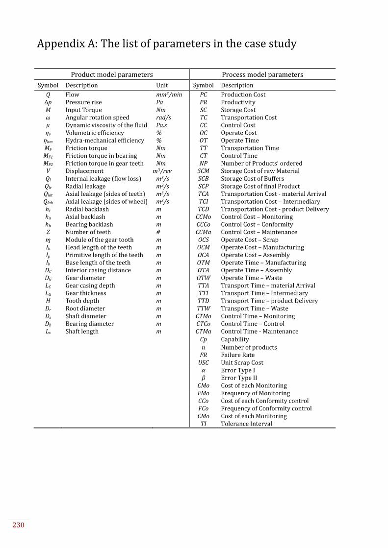
230
Appendix A: The list of parameters in the case study
Product model parameters Process model parameters
Symbol Description Unit Symbol Description
Q Flow mm3/min PC Production Cost Δp Pressure rise Pa PR Productivity M Input Torque Nm SC Storage Cost ω Angular rotation speed rad/s TC Transportation Cost µ Dynamic viscosity of the fluid Pa.s CC Control Cost ηv Volumetric efficiency % OC Operate Cost
ηhm Hydra-mechanical efficiency % OT Operate Time MF Friction torque Nm TT Transportation Time MF1 Friction torque in bearing Nm CT Control Time MF2 Friction torque in gear teeth Nm NP Number of Products’ ordered
V Displacement m3/rev SCM Storage Cost of raw Material Ql Internal leakage (flow loss) m3/s SCB Storage Cost of Buffers Qlr Radial leakage m3/s SCP Storage Cost of final Product Qlat Axial leakage (sides of teeth) m3/s TCA Transportation Cost - material Arrival Qlab Axial leakage (sides of wheel) m3/s TCI Transportation Cost – Intermediary hr Radial backlash m TCD Transportation Cost - product Delivery ha Axial backlash m CCMo Control Cost – Monitoring hb Bearing backlash m CCCo Control Cost – Conformity Z Number of teeth # CCMa Control Cost – Maintenance ɱ Module of the gear tooth m OCS Operate Cost – Scrap lh Head length of the teeth m OCM Operate Cost – Manufacturing lp Primitive length of the teeth m OCA Operate Cost – Assembly lb Base length of the teeth m OTM Operate Time – Manufacturing DC Interior casing distance m OTA Operate Time – Assembly DG Gear diameter m OTW Operate Time – Waste LC Gear casing depth m TTA Transport Time – material Arrival LG Gear thickness m TTI Transport Time – Intermediary H Tooth depth m TTD Transport Time – product Delivery Dr Root diameter m TTW Transport Time – Waste Ds Shaft diameter m CTMo Control Time – Monitoring Db Bearing diameter m CTCo Control Time – Control Ls Shaft length m CTMa Control Time - Maintenance
Cp Capability n Number of products FR Failure Rate USC Unit Scrap Cost α Error Type I β Error Type II CMo Cost of each Monitoring FMo Frequency of Monitoring CCo Cost of each Conformity control FCo Frequency of Conformity control CMo Cost of each Monitoring TI Tolerance Interval

231
Appendix B: OTCS sub-models
Raw
mat
eria
l O
OperateTransport Transport
TransportOperate TransportOperate Operate
OCMOTM
OCAOTA
OCMOTM OCAOTA
OC OT
OCS
PV
PC
PP
R1
OC
TC
CCR2
SC
OCM
OCA
R7
OCS
OTM
OTAR8
R3
OT
TT
CT
NP
Fin
al p
rod
uct
Material
Arrival
Internal
movements
Product
Departure
TCITTI TCDTTDTCATTA
TC TT
Fin
al p
roduct
T
... ...
TTW
Process
value
Production cost
Productivity
R1 OC
TC
CCR2
SC
R3
OT
TT
CT
NP
TCA
TCIR5
Transport capacity
TCD
TTA
TTIR9
TTW,
Transport capacity
TTD

232
Material
StorageBuffers
Product
Storage
SCB SCPSCM
SCR
aw m
ater
ial
Fin
al p
rod
uct
S
... ...
PV
PC
PP
R1 OC
TC
CCR2
SC
R3
OT
TT
CT
NP
SCM
SCB
SCP
R4
Storage
capacity
...
Fin
al p
rod
uct
... ...
Raw
mat
eria
l
ConformityMonitoring Maintenance
CC
C
CT
CCMoCTMo CCCoCTCo CCMaCTMa
PV
PC
PP
R1 OC
TC
CCR2
SC
R3
OT
TT
CT
NP
CCMo
CCCoR6
CCMa
CTMo
CTCo
CTMa
R10

233
Appendix C: Draft of the product in case study

234
Appendix D: An overview of the IPPM approach
Product
CT
OC
Lev
el 1
CT
OC
Lev
el 2
CT
OC
Lev
el 3
CP
M-P
rod
uct
Lev
el 1
CP
M-P
rod
uct
Lev
el 2
CP
M-P
rod
uct
Lev
el 3
Pro
du
ct D
eco
mp
osi
tio
nP
rod
uct
Dec
om
po
siti
on
CT
OC
Lev
el 4
CP
M-P
rod
uct
Lev
el 4
Pro
du
ct D
eco
mp
osi
tio
n
Sy
nth
esis
Pro
du
ct
Mo
del
lin
g
OT
CS
Lev
el 1
OT
CS
Lev
el 2
OT
CS
Lev
el 3
CP
M-P
roce
ss
Lev
el 1
CP
M-P
roce
ss
Lev
el 2
CP
M-P
roce
ss
Lev
el 3
Pro
cess
Dec
om
po
siti
on
Pro
cess
Dec
om
po
siti
on
OT
CS
Lev
el 4
CP
M-P
roce
ss
Lev
el 4
Pro
cess
Dec
om
po
siti
on
Pro
cess
Mo
del
lin
g
Pro
cess
Mo
del
lin
g
Pro
cess
Mo
del
lin
g
ProcessL
evel
1L
evel
2L
evel
3L
evel
4
Pro
du
ct
Mo
del
lin
g
Pro
du
ct
Mo
del
lin
g
Sy
nth
esis
Sy
nth
esis
Sy
nth
esis
Dec
isio
n M
akin
g
Sy
nth
esis
Sy
nth
esis
Sy
nth
esis
Sy
nth
esis
Dec
isio
n M
akin
g
Ex
tern
al C
od
itio
ns
(Dec
isio
n M
akin
g)
Ex
tern
al c
on
dit
ion
s
(Dec
isio
n M
akin
g)
Pro
cess
co
st
(Dec
isio
n M
akin
g)

235
236
Maitrise de la complexité et incertitude pour l'aide à la décision en conception
intégrée produit processus par des approches de modélisations
RESUME : L'objectif principal lors de la conception et du développement de produits est d'augmenter la
valeur de ceux-ci. La Valeur comprend deux aspects : la qualité et le coût. Afin de prendre en compte ces
deux aspects, cette thèse se focalise sur la conception intégrée des produits et des processus, et en particulier
sur la complexité du processus de conception et les incertitudes associées. Cette thèse propose une approche
de modélisation systématique pour maitriser les incertitudes et gérer la complexité. Cette approche comprend
deux phases: détermination du modèle et analyse du système. La première phase contient deux propositions :
une approche de modélisation de produits basée sur la modélisation des flux d'énergie dans le cadre
méthodologique Characteristics-Properties Modelling (CPM). Cette approche donne un cadre qui permet de
facilité la transition d’une vue fonctionnelle à une vue structurelle associée à une modélisation quantitative.
La seconde proposition porte sur l’aide du concepteur lors de la conception concurrente (IPPD) où à la fois
les performances et les coûts sont pris en compte. Cette approche est basée sur le flux du processus en
respectant le même cadre (CPM), elle donne aussi un cadre pour la transition fonctionnelle / structurelle. Les
modélisations structurelles quantitatives permettent l’analyse de sensibilité, l’analyse des tolérances et
l'optimisation. L’application de l'approche est démontrée par une étude de cas industriel. Grâce à cette
approche, les caractéristiques modifiables et pertinentes du produit peuvent être déterminées. Le
tolérancement peut être intégré dans le processus de conception et son impact sur la performance du produit
peut être analysé. Les relations quantitatives du produit, du processus sont identifiées. Les incertitudes dans
les relations et dans toutes les étapes de la modélisation peuvent être élicitées et maitrisées. Cette approche
systématique donne un cadre pour le concepteur à travers le processus de conception pour prendre des
décisions dans tous les niveaux de décomposition sur la base de la fonction requise et le coût de fabrication.
L'approche est applicable tant pour la modélisation d'un produit existant (une approche d'optimisation), tant
pour la modélisation d'un nouveau produit (phase de conception conceptuelle).
Mots clés : Conception intégrée, analyse des flux, complexité, incertitude, modélisation, IPPD
Managing Complexity and Uncertainty by a Modelling Approach for Decision
Making in Integrated Product Process Design
ABSTRACT: The main objective in product design and development is to increase the value of a product.
Value includes two aspects of quality and cost. In order to take into account both aspects, this thesis aims at
Integrated Product and Process Design, especially on product design complexity and its inherent (associated)
complexities. This thesis proposes a systematic modelling approach to reduce uncertainty and manage
complexity. The approach includes two phases: model determination and system analysis. The first phase
contains two propositions: first, a product modelling approach based on energy flow modelling in the
framework of Characteristics-Properties Modelling (CPM). This approach gives a modelling framework for a
smoother transition from functional to structural views, with a quantitative modelling. The second
proposition is to help the designer for decision making in concurrent designing (IPPD) where both
performance and cost are taken into account. This approach is based on the process flows in the same
framework (CPM). The second phase is to use the determined model of phase 1 to analyse the system. So,
phase 2 includes sensitivity analysis, tolerance analysis and optimisation. An application of the approach is
demonstrated through an industrial case study. Thanks to this approach, effective modifiable characteristics
of the product on its performance are determined. Tolerancing can be integrated in design process and its
impact on the product performance can be analysed. Quantitative links in product, in process and between
product elements and process elements are identified. Uncertainty in the links and every step of modelling
can be elicited and managed. This systematic approach gives a pathway to the designer through the design
process to make decisions in every level of decomposition based on the required function and cost of
manufacturing. The approach is applicable for both modelling an existing product (optimisation approach)
and modelling a new product (Conceptual design phase).
Keywords : Product development, flow analysis, complexity, uncertainty, modelling, IPPD