Mahdi H. Almutlaq and Gary F. Margrave · AVO inversion CREWES Research Report — Volume 22 (2010)...

AVO inversion

CREWES Research Report — Volume 22 (2010) 1

Tutorial: AVO inversion

Mahdi H. Almutlaq and Gary F. Margrave

ABSTRACT

This literature review highlights most of the highly referenced work on amplitude variation with offset (AVO) from the past three decades. This review addresses some of the approximations made to the Zoeppritz equations, as well as AVO processing, AVO analysis and inversion. The purpose of this paper is not to provide details of the different AVO methods, but instead to register in chronological order the developments and briefly present the purpose and the outcome of each study. In some instances, I presented a comparison with other methods or listed advantages and disadvantages of one AVO process over the other.

INTRODUCTION

This paper provides a brief history on some of the developments of amplitude variation with offset (AVO), AVO inversion and analyses. After choosing to write a term paper on this topic, I realized that hundreds of papers and a few books have been published on AVO. This made my task very difficult. Therefore, I admit that I did not read all of the publications but I tried my best to cover some of the highly referenced ones and included some of the work done internally within the CREWES project at the University of Calgary.

Variation in seismic amplitude with change in distance between source and receiver is typically associated with changes in lithology and fluid content in rocks above and below the reflector. The term amplitude variation with offset (AVO) was first discussed in literature in 1982 when Ostrander presented his paper "Plane Wave Reflection Coefficients for Gas Sands at Nonnormal Angles of Incidence" at the 52nd annual meeting of the SEG. Since then, the subject gained popularity and became a hot topic in exploration geophysics.

AVO analysis is a technique used by geoscientists to evaluate reservoir’s porosity, density, velocity, lithology and fluid content. But in order to obtain optimum results from AVO analysis, special acquisition, processing, and interpretation techniques of the seismic data are required. The earth’s subsurface is quite complex such that different rocks have different AVO response yet these rocks are filled with the same fluid or have the same porosity.

The definition of AVO and its basic application have been outlined above. This should serve as the starting point for understanding some of what follows. In the subsequent section, I will start with the Zoeppritz equations for reflection coefficients and then highlight some of the developments to present.

1980 – 1989

When incident P-waves propagate through an interface with different medium properties on both sides, the energy of the ray is reflected and transmitted as P-waves and

Almutlaq

2 CREWES Research Report — Volume 22 (2010)

converted S-waves (figure 1). The incident angle, reflection angles, and transmitted angles, together with P and S-wave velocities on both sides of the medium obey Snell’s law as:

( ) = ( ) = ( ) = ( ) = 𝑝. (1)

p is known as the ray parameter, θ is the incident / reflected P-wave angle, 𝜃 is the transmitted P-wave angle, 𝜑 and 𝜑 are the reflected and transmitted S-wave angle respectively, 𝛼 and 𝛽 are the P- and S-wave velocities of medium 1, and finally 𝛼 and 𝛽 are the P- and S-wave velocities for medium 2.

The Zoeppritz equations, which describe the relationship between incident rays and scattered amplitudes for plane waves and a planar interface between two homogenous isotropic elastic welded halfspaces, were at the centre of discussion in the early 1980’s. They’re known to be the exact theoretical solutions for reflection coefficients yet applications to seismic data have proven to be difficult. Some of the reasons mentioned in literature are the high number of unknowns about the subsurface and the complexities of the earth. Therefore, in order to have simple solutions to reflection coefficients, approximation of the Zoeppritz equations are required. For example, Aki and Richards (1980) introduced a first order Zoeppritz approximations for the P-P (incident P-wave and reflected P-wave) reflection coefficient (Rpp) as

𝑅 (θ) ≈ (1 − 4 𝑠𝑖𝑛 𝜃) ∆ + (1 + 𝑡𝑎𝑛 𝜃) ∆ − 4 𝑠𝑖𝑛 𝜃 ∆ (2)

where 𝛼 is the average of the two P-wave velocities on both sides of the reflector, 𝛽 is the average of the two S-wave velocities on both sides of the reflector, 𝜌 is the average of the two densities on both sides of the reflector, and 𝜃 is the average of the incident and transmitted P-wave angles. ∆𝛼 = 𝛼 − 𝛼 , ∆𝛽 = 𝛽 − 𝛽 , and ∆𝜌 = 𝜌 − 𝜌 .

AVO inversion


FIG. 1: Reflection and transmission at an interface for an incident P-wave.

Ostrander (1982, 1984) demonstrated that seismic reflection amplitude versus offset can be used to distinguish gas related amplitude anomalies from other types of amplitude anomalies. He also noticed that a significant change in the Poisson’s ratio between two media has a substantial effect on the reflection coefficient for moderate angles of incidence. His work popularized the method later known as amplitude variation with offset (AVO).

An alternate simplification of the Zoeppritz equations was performed by Shuey (1985) where he transformed the variables in equation (2) from 𝛽 to 𝜎 to display the change in Poisson’s ratio. The new simplification of the Zoeppritz equations is: 𝑅 (𝜃) ≈ 𝑅 + 𝐴 𝑅 + ∆( ) 𝑠𝑖𝑛 𝜃 + ∆ (𝑡𝑎𝑛 𝜃 − 𝑠𝑖𝑛 𝜃) (3)

where 𝑅 gives the reflection coefficient at normal incidence, the second term describes 𝑅 (𝜃) at intermediate angles and the last term explains 𝑅 (𝜃) to the critical angle. 𝐴 is the amplitude at normal incidence and is defined by

𝐴 = 𝐵 − 2(1 + 𝐵 ) , 𝐵 = ∆ ∆ + ∆ (4)

where ∆𝜎 = 𝜎 − 𝜎 and 𝜎 = (𝜎 + 𝜎 )/2. Therefore this simplification includes all the relations between 𝑅 (𝜃) and elastic properties. One requirement for this simplification is a fixed Poisson’s ratio and therefore a smooth background velocity model is required. Equation (4) can also be simplified to

Incident P-wave

Reflected P-wave

θ1

φ2

Medium 1

Medium 2

Transmitted P-wave

Normal incidence =

θ=0o

α1, β1, ρ1

α2, β2, ρ2

θ1

θ2

φ1

Transmitted S-wave

Reflected S-wave

Almutlaq


𝑅 (𝜃) ≈ 𝑅 + 𝐺𝑠𝑖𝑛 𝜃 (5)

where 𝑅 gives the intercept and G is the AVO gradient (slope) obtained by performing a linear regression analysis on the seismic amplitudes.

Smith and Gidlow (1987) also derived another approximation to the Zoeppritz equations based on the Aki and Richards’ simplification. They’ve arranged the terms of equation (2). They assumed that the relative changes in property are small so that the second-order terms can be neglected and the incident angle does not reach the critical angle (90o). With that assumption, Gardner's relationship was used to eliminate the dependency on density, 𝜌 = 𝑎𝛼 / , and the following relationship between density and P-wave velocity was used

∆ ≈ ∆

(6)

such that

𝑅 (𝜃) ≈ ∆ − 4 ∆ + ∆ 𝑠𝑖𝑛 𝜃 + ∆ 𝑡𝑎𝑛 𝜃. (7)

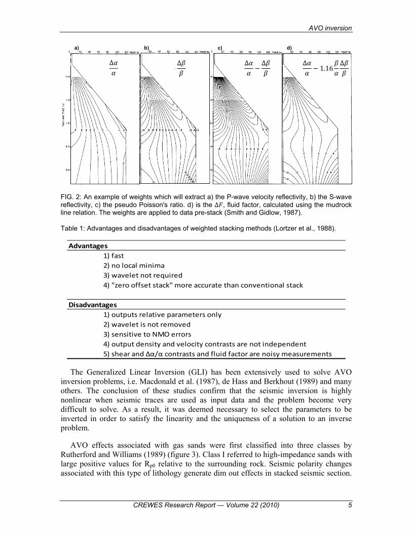
Such simplification allowed them to obtain estimates of rock properties by using a weighted stacking method (or “geo-stack”) using time- and offset-variant weights to the data samples before stacking. AVO variation was calculated using the least squares method by fitting a curve that approximates the Zoeppritz equation to all reflection amplitudes as a function of angle of incidence for each CMP gather. The outputs of this weighted stacking (geo-stack) method, using equation (7), are: ∆α α⁄ , ∆𝛽 𝛽⁄ , and ∆𝜌 𝜌⁄ (or the pseudo Poisson’s ratio) (figure 2). The solution is obtained by using the generalized linear inversion (GLI) which has the following matrix form:

∑ 𝐴 ∑ 𝐴 𝐵∑ 𝐴 𝐵 ∑ 𝐵 ∆∆ = ∑ 𝑎 𝐴∑ 𝑎 𝐵 (8)

where 𝐴 = 5 8⁄ − (1 2⁄ )( 𝛽 𝛼 )⁄ 𝑠𝑖𝑛 𝜃 + (1 2⁄ )𝑡𝑎𝑛 𝜃 and 𝐵 = −4( 𝛽 𝛼 )⁄ 𝑠𝑖𝑛 𝜃 for i = 1 ... n, where n is the number of traces contributing to the NMO-corrected CMP gather and A and B are functions of the P-wave velocity and 𝛽/𝛼 model and not of the data (Smith and Gidlow, 1987). ai is the actual amplitude of each offset sample.

Smith and Gidlow (1987) defined the “fluid factor”, ∆𝐹, as the difference between the observed ∆α α⁄ the predicted ∆α α⁄ from ∆𝛽 𝛽⁄ . Using the ‘mudrock line’ of Castagna et al. (1985), they obtained

∆𝐹 = ∆ − 1.16 ∆. (9)

Figure 2d shows the weights required to estimate ∆𝐹, where it becomes close to zero for all water-bearing rocks, but negative at the top of a gas-filled sand and positive at the bottom. Advantages and disadvantages of weighted stacks were discussed by Lortzer et al. (1988) and displayed in Table 1.

AVO inversion


FIG. 2: An example of weights which will extract a) the P-wave velocity reflectivity, b) the S-wave reflectivity, c) the pseudo Poisson's ratio. d) is the ∆𝐹, fluid factor, calculated using the mudrock line relation. The weights are applied to data pre-stack (Smith and Gidlow, 1987).

Table 1: Advantages and disadvantages of weighted stacking methods (Lortzer et al., 1988).

Advantages1) fast2) no local minima3) wavelet not required4) "zero offset stack" more accurate than conventional stack

Disadvantages1) outputs relative parameters only2) wavelet is not removed3) sensitive to NMO errors4) output density and velocity contrasts are not independent5) shear and ∆α/α contrasts and fluid factor are noisy measurements

The Generalized Linear Inversion (GLI) has been extensively used to solve AVO inversion problems, i.e. Macdonald et al. (1987), de Hass and Berkhout (1989) and many others. The conclusion of these studies confirm that the seismic inversion is highly nonlinear when seismic traces are used as input data and the problem become very difficult to solve. As a result, it was deemed necessary to select the parameters to be inverted in order to satisfy the linearity and the uniqueness of a solution to an inverse problem.

AVO effects associated with gas sands were first classified into three classes by Rutherford and Williams (1989) (figure 3). Class I referred to high-impedance sands with large positive values for Rp0 relative to the surrounding rock. Seismic polarity changes associated with this type of lithology generate dim out effects in stacked seismic section.

∆𝛼𝛼 = ∆𝛽𝛽 ∆𝛼𝛼 − ∆𝛽𝛽 ∆𝛼𝛼 − 1.16 𝛽𝛼 ∆𝛽𝛽a) b) c) d)

Almutlaq


Class II referred to near-zero impedance contrast sands or nearly the same impedance as the surrounding shale where Rp0 values are near zero. Class III referred to low-impedance sands by comparison to the surrounding shale with negative values for Rp0. Typically, class I AVO anomalies are related to dim spots and Class III AVO anomalies are linked to bright spots. On the other hand, Class II AVO responses cover the range of dim spots and phase reversals in a normal incidence (NI) reflectivity analysis which will be discussed later.

FIG. 3: Zoeppritz P-wave reflection coefficients for a shale/gas-sand interface for a range of Rp0 values. The Poisson’s ratio and density of the shale were assumed to be 0.38 and 2.4 g/cm3, respectively. The Poisson’s ratio and density of the gas sand were assumed to be 0.15 and 2.0 g/cm3, respectively (Rutherford and Williams, 1989).

1990 - 1999

Stewart (1990) extended the weighted stacking method (Smith and Gidlow, 1987) that utilized the P-P seismic data only to include P-P and P-SV reflectivities. Though theoretic, Stewart was able to relate rock properties (𝛼, 𝛽, 𝜌) to elastic-wave reflectivities and outlined the advantages of jointly inverting for P-P and P-S data.

Almost all AVO studies found that any attempt of forward modeling to predict AVO responses in field data fails unless shear-wave velocity is available (Burnett, 1990). Processing techniques have advanced to overcome some of the difficulties for AVO analysis. For example, areas with complex structures or significant dips require sophisticated processing technique, such as pre-stack migration (de Bruin et al., 1990). Other challenges faced by geophysicists when working with AVO analysis were those

AVO inversion


studied by Swan (1991) where he pointed out five sources of errors for AVO intercept/gradient measurements, including velocity estimation, the most serious one, and NMO stretch. Further on calculating AVO intercept and gradient, Walden (1991) demonstrated that damage done by outliers to the amplitude profiles can be prevented by using robust regression techniques.

Several Seismic data processing schemes for AVO analysis were reported in the literature and authors like Castagna and Backus (1993) added that when processing seismic data, careful balancing of two objectives: 1) noise suppression versus 2) not biasing or corrupting reflectivity variation with offset, are very critical.

In 1994, Fatti et al. improved the Geo-stack method (first introduced by Smith and Gidlow, 1987) by incorporating the density changes instead of using the empirical relationship between 𝛼 and 𝜌. They also rearranged the Aki-Richard’s approximation so that

𝑅 (𝜃) = (1 + 𝑡𝑎𝑛 𝜃) ∆ − 4 𝑠𝑖𝑛 𝜃 ∆ − 𝑡𝑎𝑛 𝜃 − 2 𝑠𝑖𝑛 𝜃 ∆.(10)

For angle of incidence less than 35 degrees and α β⁄ ratio between 1.5 and 2.0, the above equation simplifies to

𝑅 (𝜃) = (1 + 𝑡𝑎𝑛 𝜃) ∆ − 4 𝑠𝑖𝑛 𝜃 ∆. (11)

Acquisition of converted-wave (P-S) seismology became important in the early 1990's. For example, Lawton (1994) discussed the design of 3C-3D surveys. Processing of converted-waves was reported by Cary (1994) for 3-D surveys. Larson and Stewart (1994) developed techniques of interpreting converted-waves data in 3-D. Moreover, Stewart et al. (1995) calculated changes in Poisson’s ratio, incompressibility, and the Lame’ parameters from the changes in normalized velocity and density from P-P and P-S reflectivity coefficients.

Developments to the Shuey’s approximations were made possible by Verm and Hilterman (1995). They noticed that when the ratio of 𝛽 𝛼⁄ is 0.5 and the terms below 30o are dropped, then the Shuey’s approximation can be reduced to two terms, a normal-incidence reflectivity term (NI), and a far-offset reflectivity term (PR), expressed as:

𝑅(𝜃) ≈ 𝑁𝐼 cos(𝜃) + 𝑃𝑅 sin (𝜃) (12)

where 𝐼 = (𝛼 𝜌 − 𝛼 𝜌 ) (𝛼 𝜌 + 𝛼 𝜌 )⁄ = 𝑅 , and 𝑃𝑅 = (𝜎 − 𝜎 ) (1 − 𝜎 )⁄ .

They noted that plotting NI versus PR reflectivities, figure 4, has the following features:

1) Shale/shale reflections (green) cluster along a -45o line,

2) Shale/water-wet sands and water-wet sands/shale reflections group along the shale line, but on the outside (yellow),

3) Shale/gas sands and gas sands/shale reflections lie near the PR axis (red).

Almutlaq


FIG. 4: Crossplot of NI-PR reflectivity traces representing a gas-saturated model (Verm and Hilterman, 1995).

Verm and Hilterman (1995) noted that lithologic clusters overlapping the NI axis are large and therefore an NI section is not considered a good lithology discriminator. To overcome this color coding of lithology, the authors tested a method that represent the lithology by a range of numerical values. They studied this on a class 2 AVO reflector in a sand/shale sequence. They noted that in order to discriminate class 2 AVO anomalies on the NI*PR section, a transformation is required to the NI and PR reflectivity which is a rotation of about 45o. Such rotation to the NI and PR reflectivities make class 2 gas sand behaves as class 3 (figure 5).

Wet Sands

Gas Sands

Shale

AVO inversion


FIG. 5: NI*PR product before rotation (a), after rotation (b), and the axis of NI and PR before and after rotation (c) where a class 2 AVO response behaved as a class 3 response after rotation (Verm and Hilterman, 1995).

It has been recognized that AVO analysis is often limited to areas of relatively flat structure. Layers with dip and diffractions due to faults are generally not analyzed for AVO. Since migration is routinely used to focus seismic sections for structural effects, it can be utilized so that AVO analysis can be performed in complex structural areas (Mosher et al., 1996). There are several techniques for migrating data in the pre-stack domain, but the one used by Mosher et al. was the common angle migration since it was proven to preserve amplitude as a function of angle. The authors emphasized a special processing flow for the migration-inversion in time domain, but prior to that, two things have to be considered, first the migration is done on the pre-stack data and secondly attention must be given to the characteristics of the seismic amplitude. Generally there are three steps to process the uncollapsed pre-stack time migration:

1) Forward discrete Radon transform (figure 6b) using the following equation

𝑔 = [𝐑𝐑𝐓 ] 𝐑𝑓 (13)

where 𝑔 represents the data in the transform domain, R is a matrix operator defined as

𝑅 = 𝑒 (14)

and f represents the observed seismic data in frequency and space and is defined as follow

a b

c

Almutlaq


𝑓(𝑥, 𝜔) = 𝑹𝑻(𝜔, 𝑝, 𝑥)𝑔(𝜔, 𝑝). (15)

2) Post-stack time migration of common offset ray parameter (p) sections. The velocity used is the stacking velocity divided by the cosine of the incident angle (figure 6c).

3) Inverse discrete Radon transform using equation 15 to return data back to time, offset, and midpoint (Figure 6d).

Figure 7 shows an example of synthetic data before and after migration. After migration, diffractions have been collapsed and dipping reflector is properly located. At the bottom of figure 7, the authors show peak amplitude as a function of offset for a time window containing the dipping reflector before and after migration. The correct amplitude is computed using the relationship given by Shuey in equation 3 (the first two terms only) and is displayed in solid line. AVO response is masked by interference from the point diffractor and residual moveout but after migration a correct response is obtained (Mosher et al., 1996).

FIG. 6: Migration-inversion processing flow. Input data in time, midpoint, and offset (a) are transformed over offset to the (𝜏 − 𝑝) domain (b). Migration of common p sections (c) collapses diffractions and corrects for dip. Data are inverse transformed after migration (d) and then normal moveout is applied (e) (Mosher et al., 1996).

AVO inversion


FIG. 7: Synthetic example with a point diffractor, dipping reflector, and flat reflector. Two stacks are shown above before and after migration. The bottom figures show AVO response of the dipping reflector before and after migration where the correct response is displayed in solid line (Mosher et al., 1996).

On top of the three-category classifications developed earlier by Rutherford and Williams, Castagna and Swan (1997) propose an additional category (Class IV). Class IV describe a low impedance gas sands where reflection coefficients decrease with increasing offset (figure 8). They also suggested that classification of hydrocarbon bearing sands should be based on intercept versus gradient cross plot instead of the NI-PR plot.

Almutlaq


FIG.8: Classification of AVO responses (previously discussed by Rutherford and Williams, 1989) with the addition of Class 4 by Castagna and Swan (1997) (plot modified by Feng and Bancroft, 2006).

At the 1997 CSEG convention, Goodway et al. presented a paper on "Improved AVO fluid detection and lithology discrimination using Lame' Petrophysical Parameters from P and S inversions". They examined the effect hydrocarbon has on Lame's parameters (incompressibility, 𝜆, and shear modulus, 𝜇) where they found that these Lame's parameters were very sensitive to hydrocarbon saturation compared to 𝛼, 𝛽 and 𝛼 𝛽⁄ . Using equation (11), the P and S-wave reflectivities are extracted and employed to calculate the Lame's parameters. Goodway et al. (based on Castagna’s work) indicated that the bulk modulus,𝜿, known to be imbedded into the P-wave velocity term, links the velocity and the rock properties for pore fluid detection. It is also known that this bulk modulus and the P-wave velocity have the most sensitive pore fluid indicator 𝝀 diluted by changing the rock matrix indicator, 𝝁, as given by: α = (𝜆 + 2𝜇) 𝜌⁄ = (𝜅 + (4/3)𝜇) 𝜌⁄ and β = 𝜇 𝜌⁄ . Goodway et al. suggested to use the modulii/density relationship to velocities or impedances instead of the standard approaches which are seen to be either insensitive or complex as rock property indicators. Therefore, the new form is given by: 𝐼 = (α𝜌) = (𝜆 + 2𝜇)𝜌 and 𝐼 = (β𝜌) = 𝜇𝜌. To extract Lame parameters 𝝀 and 𝝁 from logs with measured density 𝝆, or 𝝀𝝆 and 𝝁𝝆 from seismic without known density, the relationship is given by: 𝜆 = α ρ − 2β ρ, 𝜇 =β 𝜌,and λρ = I − 2I , 𝜇𝜌 = I (Goodway et al., 1997).

Interpretation of AVO anomalies and describing the effects on rock and pore fluid properties using slopes and intercept cross-plots was examined by Foster and Keys (1999). They worked an exact expression for intercept (A) and slope (B) given a small perturbation in velocity and density at a reflecting interface:

AVO inversion


𝐴 = ∆ + ∆ (16a)

𝐵 = (1 − 8𝛾 )𝐴 − 4𝛾∆𝛾 + (4𝛾 − 1) ∆ (16b)

and if the ratio 𝛾 (𝛾 = 𝛽/𝛼) is close to 0.5 (assuming small perturbations in elastic properties at the reflecting interface), then

𝐵 = (1 − 8𝛾 )𝐴 − 4𝛾∆𝛾 (17)

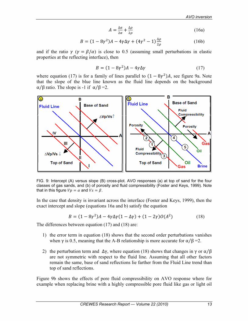
where equation (17) is for a family of lines parallel to (1 − 8𝛾 )𝐴, see figure 9a. Note that the slope of the blue line known as the fluid line depends on the background α β⁄ ratio. The slope is -1 if α β⁄ =2.

FIG. 9: Intercept (A) versus slope (B) cross-plot. AVO responses (a) at top of sand for the four classes of gas sands, and (b) of porosity and fluid compressibility (Foster and Keys, 1999). Note that in this figure 𝑉𝑝 = 𝛼 and 𝑉𝑠 = 𝛽.

In the case that density is invariant across the interface (Foster and Keys, 1999), then the exact intercept and slope (equations 16a and b) satisfy the equation

𝐵 = (1 − 8𝛾 )𝐴 − 4𝛾∆𝛾(1 − ∆𝛾) + (1 − 2𝛾)𝑂(𝐴 ) (18)

The differences between equation (17) and (18) are:

1) the error term in equation (18) shows that the second order perturbations vanishes when γ is 0.5, meaning that the A-B relationship is more accurate for α β⁄ =2.

2) the perturbation term and ∆γ, where equation (18) shows that changes in γ or α β⁄ are not symmetric with respect to the fluid line. Assuming that all other factors remain the same, base of sand reflections lie farther from the Fluid Line trend than top of sand reflections.

Figure 9b shows the effects of pore fluid compressibility on AVO response where for example when replacing brine with a highly compressible pore fluid like gas or light oil

Almutlaq


results in reducing 𝛼. 𝛽 on the other hand is not affected by the type of fluid. Another rock property that alters AVO response is the rock porosity, i.e. an increase in porosity results in a decreasing 𝛼, 𝛽 and density.

AVO analysis is mainly achieved using P-wave data due to the lack or poor quality of S-wave data. But advances in seismic data acquisition made it possible to acquire high-quality S-wave data and use these measurements to obtain rock property. A real data example using P- and S-waves jointly in AVO analysis to estimate elastic parameters for reservoir characterization, particularly fluid contact detection and pore fill distinction was presented by Jin (1999). In his study, the obtained elastic parameters responded differently depending on the nature of lithology and fluid content. Arrows in Figure 10 indicate the bottom of the reservoir. Note that the P-wave data don't explain the reservoir geometry as well as the S-wave data. Note also that more information about the reservoir can be obtained from the S-wave velocity and density.

AVO inversion


FIG. 10: Contrasts of elastic parameters from P-P and P-S AVO inversion (Orange arrows indicate the fluid contact) (Jin, 1999).

Larsen (1999) presented in his thesis the simultaneous inversion of P-P and P-S seismic data as well as obtained estimates of Ip and Is. This method utilized weighted and migrated stacks and recursive inversion. In his work, he was able to demonstrate that this inversion method can be extended and applied to 3-term parameter inversion giving 𝛼, 𝛽 and density estimates of the subsurface. The inversion of the Blackfoot 3C-3D data demonstrated that the P-P weighted stacking method does not effectively predict the size of the upper incised-valley. However, the simultaneous method clearly maps the upper incised valley (Figure 11).

Almutlaq


FIG. 11: Weighted impedance reflectivity stacks for the P-P only (left) and simultaneous inversion methods (right) (Larsen, 1999). The left display illustrates clearly the channel at the lower half of the display with five producing wells (black filled circles) penetrated the channel.

2000 – 2009

Interpretation of AVO cross-plot can be simplified by considering the observed displacements from the background trend (BT) which are the result of summing the displacements related to the specific rock properties contrasts (Kelly and Ford, 2000). They defined the displacement as the vector from the origin to a cross-plot or between two cross-plots. They also considered three types of displacements: 1) interface displacement, 2) spatial displacement (contrast in rock properties between two locations) and 3) temporal displacement (contrast in rock properties between two times at a single location). They argue that cross-plotting the P-S AVO attributes (D0 vs. D1) has several advantages over the traditional P-P attribute cross-plots (slope vs. intercept). One of the advantages is that cross-plot displacement can be decomposed into its components because of the clear distinction between density and shear velocity. The D0 and D1 are the P-S AVO attributes coefficients defined by 𝐷0 = ∆𝜌 𝜌⁄ and 𝐷1 = ∆𝛽 𝛽⁄ .

Figure 12 illustrates the cross-plot displacements associated with the density and shear-wave velocity for two models: shale on top of gas filled reservoir sand and shale on top of brine filled reservoir sand.

AVO inversion


FIG. 12: shows P-S attribute cross-plot displacements for a D0 vs. D1 (a), Shale/Gas-filled Sand displacement and the rock property displacement (b), and Shale/Brine-filled Sand displacement with the additional displacement due to hydrocarbon substitution. The Background Trend (BT) for Shale/Brine Sand is illustrated (Kelly and Ford, 2000).

More progress has also been made on AVO inversion for elastic parameters. The paper by Bale et al. (2001) to estimate the reflectivity as a function of incidence angle is one example of the continuous development. Their approach can simply be described as a time-dependent transformation from offset to incidence angle at the reflector. This is considered a fundamental step in AVO analysis. They have determined the angles used to compute the AVO attributes using the non-hyperbolic moveout equation. For PS reflections, they have used the P-wave equation and information about the shear velocities obtained from common conversion point (CCP) position. The study included the impact of the vertical heterogeneity and VTI on AVO attributes which found to be significant. Figure 13 shows a comparison of hyperbolic and non-hyperbolic offset-to-angle mapping for PP and PS AVO responses.

a b

c

Almutlaq


FIG. 13: AVO responses for (a) PP reflection and (b) for PS conversion. Differences result from the different offset-to-angle mappings: stretches are observed on the non-hyperbolic curve compared to the hyperbolic. For the PS case (b), different results are compared to account for the affect of VTI (Bale et al., 2001).

The intention of processing seismic data for AVO specific analysis is to be able to extract rock properties from seismic data in addition to the structural image. To do an AVO analysis is to fit a gradient to amplitude observations over a range of offsets. Therefore, when processing seismic data, special attention must be considered to preserve this variation to amplitude due to lithology and fluid contents. According to Yilmaz (2001), there are three important processing steps for AVO analysis.

• The relative amplitudes of the seismic data must be preserved throughout the analysis in order to recognize the amplitude variation with offset.

• Broad band signal must be retained in the data with a flat spectrum.

• Pre-stack amplitude inversion must be applied to common-reflection point (CRP) gathers to obtain the AVO attributes.

New linearized AVO inversion using Bayesian technique was developed in order to obtain a posterior P-wave velocity, S-wave velocity and density distributions (Buland and Omre, 2003). Other elastic parameters (acoustic impedance, shear impedance, and ratio of P- and S-wave velocities) distributions can also be obtained (Buland and Omre, 2003). The solution of the AVO inversion was given by a Gaussian posterior distribution. This type of linearized AVO inversion was tested on synthetic and field data where the synthetic data with S/N ratio of 105 show high correlation between the estimated and the correct mode. The same thing with the inversion of the field data where there was a good agreement with the well logs data, but there was also high uncertainty (Buland and Omre, 2003). The inversion results of the synthetic data set are shown in figure 14 with S/N ratio 105 showing the maximum a posteriori model (MAP) solution with 0.95 prediction interval for P- and S-wave velocities, density, acoustic impedance, shear impedance, and P- to S-impedance ratio. The solutions of the first three parameters are analytically obtainable, whereas the stochastic simulation from the posterior distribution is used for the last three (Buland and Omre, 2003). The red dashed line in figure 14 shows the 0.95

AVO inversion


intervals of the prior model. Note that with this low noise level, all inverted parameters are retrieved perfectly with low uncertainty. Figure 15 illustrates the MAP results in the well location and the 0.95 prediction intervals. In this solution, the acoustic impedance and the P-wave velocity are the best solved parameters. The other parameters were inverted and they show good agreement with well logs, but the uncertainty is high due to their dependence on the prior model and the noise level (Buland and Omre, 2003).

FIG. 14: The MAP solution (thick blue line) of the synthetic data with S/N ration 105 and 0.95 prediction interval (thin blue lines), the true model profile (black line), and 0.95 prior model interval (red dotted lines) (Buland and Omre, 2003).

Almutlaq


FIG. 15: The MAP solution (thick blue line) in the well location with 0.95 prediction interval (thin blue lines), the well log (black line), and 0.95 prior model interval (red dotted lines) (Buland and Omre, 2003).

In his PhD thesis, Downton (2005) managed to develop a constrained three term AVO inversion following a Bayesian approach. He found that constraints are influenced by the noise to signal level, where greater influence of constraints is obtained with low noise level. Downton also estimated density reflectivity along with the corresponding reliability displays. His approach was different from others in that he used a linear approximation without including the higher order reflectivity terms in the Zoeppritz equations. In

AVO inversion


addition, he investigated the error associated with the linear operator and showed that random errors in the 𝛼/𝛽 ratio and offset-to-angle mapping lead to second order random error (usually neglected compared to error arising from random noise). Other errors arising from seismic data preconditioning such as the effect of NMO stretch and offset dependent tunning on the AVO inversion were also examined. He found that reflectivity estimates for Class I and II gas sand anomalies were not distorted by the NMO stretch and offset dependent tunning, however Class III and IV gas sand anomalies were significantly distorted for large angles (i.e. greater than 45 degrees).

Linear AVO inversion of compressional and converted shear surface seismic data was examined by Mahmoudian (2006). The purpose was to obtain the physical properties of three parameters - compressional impedance, shear impedance, and density. Due to the ill-posed nature of the inverse problem, damped SVD (singular value decomposition) method, as opposed to least square method, was used to stabilize the AVO inversion. The stability of the three term AVO inversion remains to be an issue. The stability of the two-term solution is obtained by using different constraints which lead to many two-parameter methods (Ursenbach and Stewart, 2008). Ursenbach and Stewart (2008) derived expressions for the inversion error of each method where such expressions allow for conversion of solutions of any two-parameter method to another two-parameter method. According to them, the only condition for such formulas to work is that the maximum angle of incidence be at least a few degrees less than the critical angle.

In a recent study on AVO inversion, Wilson et al. (2009) presented a new technique where from the reflection data, the frequency dependent impedance contrasts can be determined. This study assumes based on recent modeling that layers exhibiting velocity dispersion have reflection coefficients varying with frequency. The hope is to make use of this study in discriminating fluids. The algorithm proved robust on synthetic data, however much work is needed to overcome the effect of tunning and NMO stretch (Wilson et al., 2009).

CONCLUSIONS

A brief presentation of AVO over the past three decades was included in this paper. The topics ranged from simplification of the Zoeppritz equations to AVO analysis, AVO processing and inversion. The summary provided includes, in chronological order from 1980 to 2009, some of the highly referenced work on AVO.

Towards the end of this review, I realized that AVO cannot be perfectly reviewed in a small report like this one. Instead, it requires a book with many chapters discussing the different topics of AVO and how to integrate all of these techniques to give the geoscientist a better image of the subsurface.

So towards the end of this paper, it is fare to ask what is the future trend of AVO? Although not discussed in this paper, time-lapse AVO is a research topic that shows promise. Repeated seismic surveys are conducted to evaluate changes in fluid contacts and AVO techniques can help in this tremendously.

Almutlaq


ACKNOWLEDGMENTS

The first author would like to acknowledge Dr. Gary Margrave for his inversion course and his insightful hints on how to write and tackle a big topic such as AVO. Both authors would like to thank the sponsors of the CREWES project for their continued support.

REFERENCES

Aki, K., and Richards, P.G., 1980, Quantitative seismology: Theory and methods: W. H. Freeman and Co. Bale, R., Leany, S., and Dumitru, G., 2001, 2001, Offset-to-angle transformations for PP and PS AVO

analysis: 71st Ann. Intern. Mtg., SEG, Expanded Abstracts. de Bruin, C.G.M., Wapenaar, C.P.A., and Berkhout, A.J., 1990, Angle-dependent reflectivity by means of

pre-stack migration: Geophysics, 55, 1223-1234. Buland, A. and Omre, H., 2003, Bayesian linearized AVO inversion: Geophysics, 68, 185-198. Burnett, R., 1990, Seismic amplitude anomalies and AVO analysis at Mestena Grande Field, Jim Hogg Co.,

Texas, Geophysics, 55, 1015-1025. Cary, P.W., 1994, 3-D converted-wave seismic processing: CREWES Research Report, Vol. 6. Castagna, J.P. and Backus, M.M., 1993, AVO analysis-tutorial and review, in Castagna, J.P. and Backus,

M.M., eds, Offset-dependent reflectivity - Theory and practice of AVO analysis: SEG, 3-37. Castagna, J.P. and Swan, H.W., 1997, Principles of AVO crossplotting: The Leading Edge, 16, 337-342. Downton, J.E., 2005, Seismic parameter estimation from AVO inversion: Ph.D. Thesis, University of

Calgary, Dept. of Geology and Geophysics. Fatti, J.L., Smith, G.C., Vail, P.J., and Levitt, P.R., 1994, Detection of gas in sandstone resevoirs using

AVO analysis: a 3-D seismic case history using the Geostack technique: Geophysics, 59, 1362-1376.

Feng, H. and Bancroft, J.C., 2006, AVO principles, processing and inversion: CREWES Research Report, Vol. 18.

Foster, D.J., and Keys, R.G., 1999, Interpreting AVO responses: 69th Ann. Intern. Mtg., SEG, Expanded Abstracts, 748-751.

Goodway, B., Chen, T., and Downton, J., 1997, Improved AVO fluid detection and lithology discrimination using Lamé petrophysical parameters; "λρ", "μρ", & "λ/μ fluid stack", from P and S inversions: 67th Ann. Intern. Mtg., SEG, Expanded Abstracts, 183-186.

de Hass, J.C. and Berkhout, A.J., 1989, Practical approach to nonlinear inversion of amplitude versus offset information: 59th Ann. Intern. Mtg., SEG, Expanded Abstracts, 2, 839-842.

Jin, S., 1999, Characterizing reservoir by using jointly P- and S-wave AVO analysis: 69th Ann. Intern. Mtg., SEG, Expanded Abstracts, 687-690.

Kelly, M.C. and Ford, D., 2000, P-S AVO attributes and cross-plotting: 70th Ann. Intern. Mtg., SEG, Expanded Abstracts, 222-223.

Larsen, J.A., 1999, AVO inversion by simultaneous P-P and P-S inversion: M.Sc. Thesis, University of Calgary, Dept. of Geology and Geophysics.

Larson, G.A. and Stewart, R.R., 1994, Analysis of 3-D P-S seismic data: Joffre, Alberta: CREWES Research Report, Vol. 6.

Lawton, D.C., 1994, Acquisition design for 3-D converted waves: CREWES Research Report, Vol. 6. Lortzer, G.J.M., de Hass, J.C., and Berkhout, A.J., 1988, Evaluation of weighted stacking techniques for

inversion: 58th Ann. Intern. Mtg., SEG, Expanded Abstracts, 1204-1208. MacDonald, C., Davis, P. M., and Jackson, D. D., 1987, Inversion of reflection traveltimes and amplitudes:

Geophysics, 52, 606–617. Mahmoudian, F., 2006, Linear AVO inversion of multi-component surface seismic and VSP data: M.Sc.

Thesis, University of Calgary, Dept. of Geology and Geophysics. Mosher, C.C., Keho, T.H., Weglein, A.B. and Foster, D.J., 1996, The impact of migration on AVO:

Geophysics, 61, 1603-1615. Ostrander, W.J., 1982, Plane-wave reflection coefficients for gas sands at nonnormal angles of incidence:

52nd Ann. Intern. Mtg., SEG, Expanded Abstracts, 216-218. Ostrander, W.J., 1984, Plane-wave reflection coefficients for gas sands at nonnormal angles of incidence:

Geophysics, 49, 1637-1648.

AVO inversion


Rutherford, S.R. and Williams, R.H., 1989, Amplitude-versus-offset variations in gas sands: Geophysics, 54, 680-688.

Shuey, R.T., 1985, A simplification of the Zoeppritz equations: Geophysics, 50, 609-614. Smith, G.C. and Gidlow, P.M., 1987, Weighted stacking for rock property estimation and detection of gas:

Geophys. Prosp., 35, 993-1014. Stewart, R.R., Zhang, Q., and Guthoff, F., 1995, Relationships among elastic-wave values (Rpp, Rps, Rss,

Vp, Vs, ρ, σ, κ), CREWES Report, 7, 10, 1-9. Stewart, R.R., 1990, Joint P and P-SV inversion, CREWES Research Report, 2, 1990. Swan, H.W., 1991, Amplitude-versus-offset measurement errors in a finely layered medium: Geophysics,

56, 41-49. Ursenbach, C.P. and Stewart, R.R., 2008, Two-term AVO inversion: Equivalences and new methods:

Geophysics, 73, C31-C38. Verm, R. and Hilterman, F., 1995, Lithology color-coded seismic sections: The calibration of AVO

crossplotting to rock properties: The Leading Edge, 14, 847-853. Walden, A.T., 1991, Making AVO sections more robust: Geophys. Prosp., 39, 915-942. Wilson, A., Chapman, M., and Li, X.Y., 2009, Frequency-dependent AVO inversion: 79th Ann. Intern.

Mtg., SEG, Expanded Abstracts, 341-345. Yilmaz, O., 2001, Seismic Data Processing: Society of Exploration Geophysicists.

Mahdi H. Almutlaq and Gary F. Margrave · AVO inversion CREWES Research Report — Volume 22 (2010)...

Documents

Transcript of Mahdi H. Almutlaq and Gary F. Margrave · AVO inversion CREWES Research Report — Volume 22 (2010)...