Machine Perception and Learning of Complex - Reality Mining

Machine Perception and Learning of Complex Social Systems

by Nathan Norfleet Eagle

B.S., Mechanical Engineering, Stanford University 1999 M.S., Management Science and Engineering, Stanford University 2001

M.S., Electrical Engineering, Stanford University 2003 Submitted to the Program of Media Arts and Sciences,

School of Architecture and Planning, in partial fulfillment of the requirements for the degree of

DOCTOR OF PHILOSOPHY IN MEDIA ARTS AND SCIENCES at the

MASSACHUSETTS INSTITUTE OF TECHNOLOGY

May 2005 © Massachusetts Institute of Technology, 2005. All rights reserved.

Author . . . . . . . . . . . . . . . . . . . . . . . . . . . . . . . . . . . . . . . . . . . . . . . . . . . . . . . . . . . . . . . . . .

Program in Media Arts and Sciences Month Day, 2005

Certified by . . . . . . . . . . . . . . . . . . . . . . . . . . . . . . . . . . . . . . . . . . . . . . . . . . . . . . . . . . . . . .

Alex P. Pentland Professor of Electrical Engineering and Computer Science

Thesis Supervisor

Accepted by . . . . . . . . . . . . . . . . . . . . . . . . . . . . . . . . . . . . . . . . . . . . . . . . . . . . . . . . . . . . . .

Andrew B. Lippman Chair

Departmental Committee on Graduate Students Program in Media Arts and Sciences

2


by Nathan Norfleet Eagle

Submitted to the Program of Media Arts and Sciences, School of Architecture and Planning,

on April, 29, 2005, in partial fulfillment of the requirements for the degree of DOCTOR OF PHILOSOPHY

Abstract

The study of complex social systems has traditionally been an arduous process, involving extensive surveys, interviews, ethnographic studies, or analysis of online behavior. Today, however, it is possible to use the unprecedented amount of information generated by pervasive mobile phones to provide insights into the dynamics of both individual and group behavior. Information such as continuous proximity, location, communication and activity data, has been gathered from the phones of 100 human subjects at MIT. Systematic measurements from these 100 people over the course of eight months have generated one of the largest datasets of continuous human behavior ever collected, representing over 300,000 hours of daily activity. In this thesis we describe how this data can be used to uncover regular rules and structure in behavior of both individuals and organizations, infer relationships between subjects, verify self-report survey data, and study social network dynamics. By combining theoretical models with rich and systematic measurements, we show it is possible to gain insight into the underlying behavior of complex social systems.

Thesis Supervisor: Alex P. Pentland

Title: Toshiba Professor of Media Arts and Sciences, MIT.

3


by Nathan Eagle

Thesis Committee:

Advisor: . . . . . . . . . . . . . . . . . . . . . . . . . . . . . . . . . . . . . . . . . . . . . . . . . . . . . . . . . . . . . . . . . .

Alex (Sandy) Pentland Toshiba Professor of Media Arts and Sciences

Massachusetts Institute of Technology

Thesis Reader . . . . . . . . . . . . . . . . . . . . . . . . . . . . . . . . . . . . . . . . . . . . . . . . . . . . . . . . . . . . . .

Pattie Maes Professor of Media Arts and Sciences

Massachusetts Institute of Technology

Thesis Reader . . . . . . . . . . . . . . . . . . . . . . . . . . . . . . . . . . . . . . . . . . . . . . . . . . . . . . . . . . . . . .

J. Richard Hackman Professor of Social and Organizational Psychology

Harvard University

4

Acknowledgments

This thesis is the product of many collaborations. My primary collaborator over the last few years

has been Alex (Sandy) Pentland. I feel lucky to have landed in his group four years ago and am

looking forward to continuing our collaborations. Additionally, I would like to acknowledge the

rest of Sandy’s Human Dynamics group at the MIT Media Lab: Juan Carlos Barahona, Joost

Bonsen, Ron Caneel, Wen Dong, Jon Gips, Anmol Madan, and Michael Sung – as well as former

members including Martin Martin, Rich DeVaul, Brian Clarkson, Sumit Basu and Tanzeem

Choudhery. While it has been a diverse and evolving group, it has remained unified around our

principle research direction – modeling human dynamics in such a way as to build applications

that better support both the individual and the group.

My many collaborators deserve particular acknowledgement. Mika Raento has been the principal

architect of the software we used to collect the Reality Mining dataset. Tony Pryor, Greg

Sterndale and Pedro Yip have been the driving forces behind the development of Serendipity.

David Lazer, a Political Science professor at Harvard University, has been a wonderful social

science resource to bounce ideas off of. Professor Judith Donath has also been instrumental in my

thinking about the privacy implications of this type of research. Other faculty members that have

shaped my thinking about this research direction include Tom Allen, Pattie Maes, and Richard

Hackman. Aaron Clauset and Leon Dannon have been two great physicist friends and

collaborators on complex network analysis. Push Singh has been a wonderful idea generator and

influenced my thinking in areas from artificial intelligence to social relationships. Caroline

Buckee has proven to be one of the best science editors and writers I have worked with – as well

as someone who shares my enthusiasm for entropy. Stephen Guerin of the Red Fish Group is

responsible for the wonderful visualizations of this dataset, and Mike Lambert has been

responsible for designing our diary application. I’d also like to acknowledge Max Van Kleek, Bo

Morgan, Lauren Oldja, and Sanith Wijesinghe.

This research would not be possible without the generous donations from Nokia. In particular

Harri Pennanen, Kai Mustonen, Hartti Suomela, Saku Hieta, Kari Pulli, Peter Wakim, Franklin

Reynolds, Suvi Hiltunen, Ken Beausang, and Timo Salomaki have all been instrumental in the

research and have certainly played a large role as a Media Lab sponsor.

5

Many people who work at the Media Lab have also played a great role in shaping and supporting

this research direction. The Media Lab administrators (both past and present) are certainly

deserving of recognition: Elizabeth Hartnett, Mary Heckbert, Linda Peterson, and Pat Solakoff.

There are simply too many Media Lab friends to acknowledge, but a partial list would include:

Aisling Kelliher, Andrea Lockerd Thomaz, Andrew Sempere, Anindita Basu, Ashish Kapoor,

Barbara Barry, Ben Vigoda, Brad Lassey, Brian Chow, Cameron Marlow, Cory Kidd, Dave

Merrill, Geva Patz, Jeana Frost, Joannie DiMicco, Josh Lifton, Lily Shirvanee, Mat Laibowitz,

Matt Reynolds, Michael Rosenblatt, Saul Griffith, Stacie Slotnick, and Win Burleson.

Final acknowledgement should go out to both my family, and of course, the intrepid group of

Reality Mining subjects.

6

Table of Contents ABSTRACT .................................................................................................................................................. 2

ACKNOWLEDGMENTS............................................................................................................................ 4

TABLE OF CONTENTS............................................................................................................................. 6

LIST OF FIGURES.................................................................................................................................... 11

PREAMBLE ............................................................................................................................................... 18

CHAPTER 1 INTRODUCTION ......................................................................................................... 20

1.1 TRADE-OFFS IN TRADITIONAL SOCIAL DATA GATHERING ........................................................... 20

1.2 NEW INSTRUMENTS FOR BEHAVIORAL DATA COLLECTION ....................................................... 22

1.3 CONTRIBUTIONS......................................................................................................................... 22

1.4 THESIS ROADMAP ...................................................................................................................... 23

CHAPTER 2 BACKGROUND ............................................................................................................ 26

2.1 COMPLEX SOCIAL SYSTEMS....................................................................................................... 27

2.2 COMPLEX NETWORKS ................................................................................................................ 27

2.3 SOCIAL PROXIMITY SENSING ..................................................................................................... 29

2.3.1 Technology Overview ........................................................................................................... 29

2.3.2 Reality Mining as a Proximity Sensing Technology ............................................................. 32

2.4 SOCIAL SOFTWARE .................................................................................................................... 32

2.4.1 The Opportunity for Mobile Social Software........................................................................ 33

2.5 SHORTCOMINGS IN SOCIAL SCIENCE .......................................................................................... 34

2.5.1 Reliance on Self-Report Measures........................................................................................ 34

2.5.2 Absence of Longitudinal Data .............................................................................................. 35

7

2.5.3 Study of macro-networks ...................................................................................................... 36

CHAPTER 3 METHODOLOGY & RESEARCH DESIGN............................................................. 38

3.1 HUMAN SUBJECTS APPROVAL.................................................................................................... 38

3.2 PARTICIPANTS............................................................................................................................ 39

3.2.1 Recruitment........................................................................................................................... 39

3.2.2 Informed Consent ................................................................................................................. 40

3.2.3 Privacy Implications & Reactions ........................................................................................ 40

3.3 APPARATUS................................................................................................................................ 40

3.4 PROCEDURE ............................................................................................................................... 41

3.4.1 Continuous Bluetooth Scanning............................................................................................ 41

3.4.2 Cell Tower Probability Distributions ................................................................................... 43

3.5 DATA COLLECTION AND VALIDATION ....................................................................................... 46

3.5.1 Data Collection..................................................................................................................... 46

3.5.2 Data Validation .................................................................................................................... 48

3.6 THE FINAL DATASET.................................................................................................................. 51

CHAPTER 4 SENSING COMPLEX SOCIAL SYSTEMS............................................................... 52

4.1 PHONE USAGE STATISTICS ......................................................................................................... 52

4.2 REALITY MINING VS. SELF-REPORT DATA................................................................................. 54

4.3 TEAM DENSITY AND SATISFACTION........................................................................................... 56

4.4 SOCIAL NETWORK EVOLUTION .................................................................................................. 57

4.5 SAMPLING DYNAMIC NETWORKS............................................................................................... 59

8

4.5.1 Overview............................................................................................................................... 59

4.5.2 Network Metrics ................................................................................................................... 60

4.5.3 Sampling Dynamic Networks................................................................................................ 62

CHAPTER 5 ILLUSTRATIVE MODELS AND APPLICATIONS ................................................ 67

5.1 INDIVIDUAL MODELING AND APPLICATIONS.............................................................................. 67

5.1.1 The Entropy of Life ............................................................................................................... 68

5.1.2 Life Log................................................................................................................................. 72

5.1.3 Conversation Gisiting from Context and Common Sense..................................................... 74

5.2 DYADIC INFERENCE ................................................................................................................... 77

5.2.1 Human Landmarks ............................................................................................................... 78

5.2.2 Relationship Inference .......................................................................................................... 78

5.3 MODELING TEAMS & ORGANIZATIONS...................................................................................... 81

5.3.1 Team Dynamics .................................................................................................................... 82

5.3.2 Organizational Modeling & Rhythms................................................................................... 84

CHAPTER 6 EIGENBEHAVIORS..................................................................................................... 89

6.1 OVERVIEW ................................................................................................................................. 89

6.2 COMPUTING EIGENBEHAVIORS .................................................................................................. 90

6.3 EIGENBEHAVIORS OF COMPLEX SOCIAL SYSTEMS ..................................................................... 95

6.3.1 Comparing Members of a Group.......................................................................................... 97

6.3.2 Identifying Group Affiliation ................................................................................................ 98

6.4 EIGENBEHAVIORS AND UBIQUITOUS COMPUTING .................................................................... 100

9

6.4.1 Usage and Behavior-based Clustering ............................................................................... 100

6.4.2 Eigenbehaviors as Biometrics ............................................................................................ 101

6.4.3 Data Interpolation .............................................................................................................. 101

6.5 CONTRIBUTIONS....................................................................................................................... 101

CHAPTER 7 INTERVENTION: SOCIAL SERENDIPITY .......................................................... 103

7.1 THE OPPORTUNITY................................................................................................................... 103

7.1.1 Enterprise ........................................................................................................................... 104

7.1.2 Dating ................................................................................................................................. 105

7.1.3 Conferences ........................................................................................................................ 106

7.2 IMPLEMENTATION .................................................................................................................... 106

7.2.1 Serendipity & Bluedar ........................................................................................................ 107

7.3 USER STUDIES.......................................................................................................................... 107

7.3.1 Initial Deployment .............................................................................................................. 108

7.3.2 Campus Deployment........................................................................................................... 110

7.4 PRIVACY IMPLICATIONS........................................................................................................... 110

7.4.1 Privacy trade-offs for matchmaking services ..................................................................... 111

7.5 BEYOND SERENDIPITY ............................................................................................................. 112

CHAPTER 8 CONCLUSIONS .......................................................................................................... 115

8.1 PRIVACY IMPLICATIONS........................................................................................................... 115

8.1.1 The Dark-Side of Mobile Phones........................................................................................ 116

8.1.2 The Price of Privacy ........................................................................................................... 117

10

8.1.3 Towards a Privacy Compromise......................................................................................... 118

8.2 LESSONS LEARNED .................................................................................................................. 120

8.2.1 Mobile Phones & Social Science ........................................................................................ 120

8.2.2 Machine Learning using Cell Tower and Bluetooth Information....................................... 120

8.2.3 Interventions: The Introduction of an Introduction Service ............................................... 121

8.2.4 Alternate Applications: Contagion Dissemination ............................................................. 121

8.3 FINALE ..................................................................................................................................... 123

REFERENCES ......................................................................................................................................... 125

11

List of Figures

FIGURE 1. THE EVOLUTION OF SOCIAL NETWORK ANALYSIS. FIGURE 1A. WAS GENERATED FROM THE RICH,

LOW-LEVEL RELATIONSHIP DATA COLLECTED BY AN OBSERVER WATCHING THE INTERACTIONS AMONG

TWELVE EMPLOYEES IN THE WESTERN ELECTRIC COMPANY IN 1935. FIGURE 1B IS A REPRESENTATION

OF THE SOCIAL NETWORK OF HUNDREDS OF HEWLETT PACKARD EMPLOYEES COLLECTED FROM SPARSE

EMAIL DATA IN 2003............................................................................................................................ 20

FIGURE 2. THE NOKIA 6600, A SYMBIAN SERIES 60 PHONE. THIS PHONE COMES WITH 6 MB OF INTERNAL

MEMORY AND A 32MB MMC FLASH MEMORY CARD. CUSTOM APPLICATIONS CAN BE LOADED ONTO

THE PHONE FROM THE GRPS DATA NETWORK, BLUETOOTH, MEMORY CARD, OR THE INFRARED PORT.

............................................................................................................................................................ 41

FIGURE 3. METHODS OF DETECTING BLUETOOTH DEVICES – BLUEAWARE AND BLUEDAR. BLUEAWARE

(LEFT) IS RUNNING IN THE FOREGROUND ON A NOKIA 3650. BLUEAWARE IS AN APPLICATION THAT

RUNS ON SYMBIAN SERIES 60 PHONES. IT RUNS IN THE BACKGROUND AND PERFORMS REPEATED

BLUETOOTH SCANS OF THE ENVIRONMENT EVERY FIVE MINUTES. BLUEDAR (RIGHT) IS COMPRISED OF A

BLUETOOTH BEACON COUPLED WITH A WIFI BRIDGE. IT ALSO PERFORMS CYCLIC BLUETOOTH SCANS

AND SENDS THE RESULTING BTIDS OVER THE 802.11B NETWORK TO THE REALITY MINING SERVER. 42

FIGURE 4 CELL TOWER PROBABILITY DISTRIBUTIONS. THE PROBABILITY OF SEEING ONE OF 25 CELL TOWERS

IS PLOTTED ABOVE FOR FIVE USERS WHO WORK ON THE THIRD FLOOR CORNER OF THE SAME OFFICE

BUILDING. EACH TOWER IS LISTED ON THE X-AXIS AND THE PROBABILITY OF THE PHONE LOGGING IT

WHILE THE USER IS IN HIS OFFICE IS SHOWN ON THE Y-AXIS. (RANGE WAS ASSURED TO 10M BY THE

PRESENCE OF A STATIC BLUETOOTH DEVICE.) IT CAN BE SEEN THAT EACH USER ‘SEES’ A DIFFERENT

DISTRIBUTION OF CELL TOWERS DEPENDENT THE LOCATION OF HIS OFFICE, WITH THE EXCEPTION OF

USERS 4 & 5, WHO ARE OFFICEMATES AND HAVE THE SAME DISTRIBUTION DESPITE BEING IN THE

OFFICE AT DIFFERENT TIMES. ............................................................................................................... 44

FIGURE 5. THE TOP TEN BLUETOOTH DEVICES ENCOUNTERED FOR SUBJECT 9 DURING THE MONTH OF

JANUARY. THE SUBJECT IS ONLY REGULARLY PROXIMATE TO OTHER BLUETOOTH DEVICES BETWEEN

9:00 AND 17:00, WHILE AT WORK – BUT NEVER AT ANY OTHER TIMES. THIS PREDICTABLE BEHAVIOR

WILL BE DEFINED IN CHAPTER 4 AS ‘LOW ENTROPY.’ THE SUBJECT’S DESKTOP COMPUTER IS LOGGED

MOST FREQUENTLY THROUGHOUT THE DAY, WITH THE EXCEPTION THE HOUR BETWEEN 14:00 AND

15:00. DURING THIS TIME WINDOW, SUBJECT 9 IS PROXIMATE MORE OFTEN TO SUBJECT 4 THAN HIS

DESKTOP COMPUTER. ........................................................................................................................... 45

12

FIGURE 6. THE NUMBER OF PROXIMATE BLUETOOTH DEVICES FOR SUBJECT 9 FOR EACH DAY BETWEEN

SEPTEMBER 3, 2004 AND JANUARY 21, 2005. WEEKENDS ARE BANDS OF WHITE INDICATIVE OF THE

SUBJECT NOT GOING INTO WORK AND THEREFORE NOT LOGGING ANY BLUETOOTH DEVICES. THE

SUBJECT’S 9:00 – 17:00 WORK SCHEDULE IS RARELY INTERRUPTED, WITH THE EXCEPTION OF SEVERAL

DAYS IN OCTOBER DURING THE LAB’S ‘SPONSOR WEEK,’ DISCUSSED IN CHAPTER 5............................ 46

FIGURE 7. MOVEMENT AND COMMUNICATION VISUALIZATION OF THE REALITY MINING SUBJECTS. IN

COLLABORATION WITH STEPHEN GUERIN OF REDFISH INC, WE HAVE BUILT A MACROMEDIA

SHOCKWAVE VISUALIZATION OF THE MOVEMENT AND COMMUNICATION BEHAVIOR OF OUR SUBJECTS.

LOCATION IS BASED ON APPROXIMATE LOCATION OF CELL TOWERS, WHILE THE LINKS BETWEEN

SUBJECTS ARE INDICATIVE OF PHONE COMMUNICATION. ..................................................................... 52

FIGURE 8. AVERAGE APPLICATION USAGE IN THREE LOCATIONS (HOME, WORK, AND OTHER) FOR 100

SUBJECTS. THE X-AXIS DISPLAYS THE FRACTION OF TIME EACH APPLICATION IS USED, AS A FUNCTION

OF TOTAL APPLICATION USAGE. FOR EXAMPLE, THE USAGE AT HOME OF THE CLOCK APPLICATION

COMPRISES ALMOST 3% OF THE TOTAL TIMES THE PHONE IS USED. THE ‘PHONE’ APPLICATION ITSELF

COMPRISES MORE THAN 80% OF THE TOTAL USAGE AND WAS NOT INCLUDED IN THIS FIGURE............. 53

FIGURE 9. AVERAGE COMMUNICATION MEDIUMS FOR 90 SUBJECTS (APPROXIMATELY 10 OF THE SUBJECTS

DID NOT USE THE PHONES AS A COMMUNICATION DEVICE AND WERE EXCLUDED FROM THIS ANALYSIS).

THE COLORBAR ON THE RIGHT INDICATES THE PERCENTAGE EACH COMMUNICATION MEDIUM (VOICE,

TEXT, AND DATA) IS USED. ALL SUBJECTS USE VOICE AS THE PRIMARY MEANS OF COMMUNICATION,

WHILE ABOUT 20% ALSO ACTIVELY USE THE DATA CAPABILITIES OF THE PHONE. LESS THAN 10% OF

THE SUBJECTS SEND A SIGNIFICANT NUMBER OF TEXT MESSAGES........................................................ 54

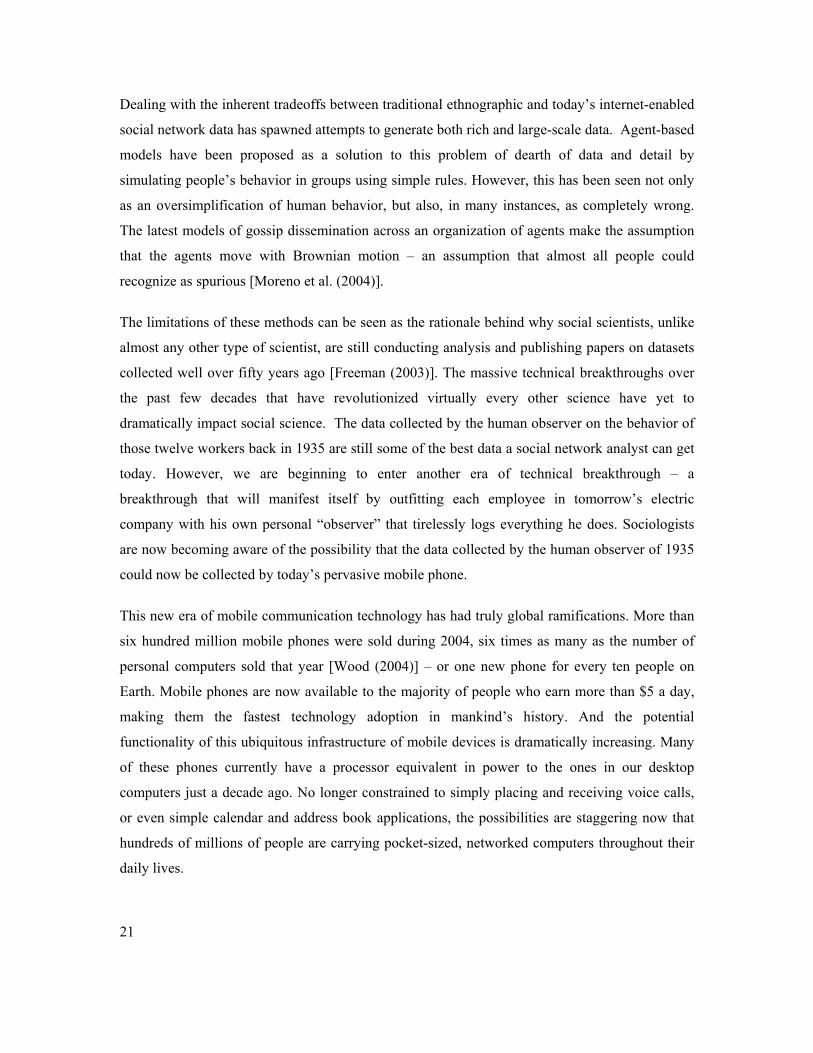
FIGURE 10. IT IS CLEAR THAT THE AVERAGE NUMBER OF UNIQUE PHONE NUMBERS LOGGED FOR THE 15

INCOMING MEDIA LAB STUDENTS AND THE 25 SLOAN STUDENTS DECAYS AT TWO VERY DIFFERENT

RATES. THE INCOMING MEDIA LAB STUDENTS ARE CLOSER TO THEIR NETWORKS’ STEADY-STATE,

WHILE THE AVERAGE GROWTH OF A TYPICAL BUSINESS SCHOOL STUDENT’S NETWORK DOES NOT

APPEAR TO HAVE SLOWED DOWN SIGNIFICANTLY WITHIN THEIR FIRST TWO MONTHS AT MIT............. 58

FIGURE 11. THE (A) MEAN DEGREE k , (B) MEAN CLUSTERING COEFFICIENT C AND (C) COMPLEMENTARY

NETWORK ADJACENCY CORRELATION 1 γ− AS A FUNCTION OF TIME FOR ∆ =1440, 480, 240, 60, 15,

5 (MINUTES) DURING THE WEEK OF 11 OCTOBER THROUGH 17 OCTOBER FOR THE CORE 66 SUBJECTS.

AS ∆ GROWS, UNDER-SAMPLING CLEARLY WASHES OUT HIGHER FREQUENCY FLUCTUATIONS .......... 63

13

FIGURE 12. THE VALUES OF EACH NETWORK METRIC (MEAN DEGREE k n/ , MEAN CLUSTERING COEFFICIENT

C AND MEAN COMPLEMENTARY ADJACENCY CORRELATION 1 γ− ) DURING THE MONTH OF OCTOBER

AS A FUNCTION OF AGGREGATION INTERVAL ∆ ; CLEARLY, THE VALUE OF EACH METRIC IS

PROPORTIONAL TO THE CHOICE OF ∆ .................................................................................................. 64

FIGURE 13. THE POWER SPECTRA OF THERE METRIC TIME SERIES AT 5∆ = MINUTES OVER THE COURSE OF

THE MONTH OF OCTOBER. THE PRINCIPLE PEAKS ARE AT 24 12∆ = , HOURS, WITH ADDITIONAL

MINOR PEAKS AT 8∆ = HOURS FOR THE MEAN DEGREE AND CLUSTERING COEFFICIENT. .................. 65

FIGURE 14. A ‘LOW-ENTROPY’ (H = 30.9) SUBJECT’S DAILY DISTRIBUTION OF HOME/WORK TRANSITIONS AND

BLUETOOTH DEVICES ENCOUNTERS DURING THE MONTH OF JANUARY. THE TOP FIGURE SHOWS THE

MOST LIKELY LOCATION OF THE SUBJECT: “WORK, HOME, ELSEWHERE, AND NO SIGNAL.” WHILE THE

SUBJECT’S STATE SPORADICALLY JUMPS TO “NO SIGNAL,” THE OTHER STATES OCCUR WITH VERY

REGULAR FREQUENCY. THIS IS CONFIRMED BY THE BLUETOOTH ENCOUNTERS PLOTTED BELOW

REPRESENTING THE STRUCTURED WORKING SCHEDULE OF THE ‘LOW-ENTROPY’ SUBJECT. ................. 69

FIGURE 15. A ‘HIGH ENTROPY’ (H = 48.5) SUBJECT’S DAILY DISTRIBUTION OF HOME/WORK TRANSITIONS AND

BLUETOOTH DEVICE ENCOUNTERS DURING THE MONTH OF JANUARY. IN CONTRAST TO FIGURE 14, THE

LACK OF READILY APPARENTLY ROUTINE AND STRUCTURE MAKES THIS SUBJECT’S BEHAVIOR HARDER

TO MODEL AND PREDICT. ..................................................................................................................... 70

FIGURE 16. ENTROPY, H(X), WAS CALCULATED FROM THE WORK, HOME, NO SIGNAL, ELSEWHERE SET OF

BEHAVIORS FOR 100 SAMPLES OF A 7-DAY PERIOD. THE MEDIA LAB FRESHMEN HAVE THE LEAST

PREDICTABLE SCHEDULES, WHICH MAKES SENSE BECAUSE THEY COME TO THE LAB MUCH LESS

REGULAR BASIS. THE STAFF AND FACULTY HAVE THE MOST LEAST ENTROPIC SCHEDULES, TYPICALLY

ADHERING TO A CONSISTENT WORK ROUTINE. ..................................................................................... 71

FIGURE 17. A HIDDEN MARKOV MODEL CONDITIONED ON TIME FOR SITUATION IDENTIFICATION. THE MODEL

WAS DESIGNED TO BE ABLE TO INCORPORATE MANY ADDITIONAL OBSERVATION VECTORS SUCH AS

FRIENDS NEARBY, TRAVELING, SLEEPING AND TALKING ON THE PHONE. ............................................. 72

FIGURE 18. LIFELOG - AUTOMATIC DIARY GENERATION. LIFELOG PROVIDES A VISUALIZATION OF THE DATA

FROM THE REALITY MINING PHONE LOGS AND INFERENCES. IT HAS ALSO INCORPORATED THE ABILITY

TO PERFORM “LIFE QUERIES,” ALLOWING THE USER TO SEARCH THROUGH PREVIOUS EVENTS AND

EXPERIENCES. ...................................................................................................................................... 74

14

FIGURE 19. FRIENDSHIP (LEFT) AND DAILY PROXIMITY (RIGHT) NETWORKS SHARE SIMILAR STRUCTURE.

BLUE CIRCLES REPRESENT INCOMING SLOAN BUSINESS SCHOOL STUDENTS. RED TRIANGLES, ORANGE

DIAMONDS AND WHITE SQUARES REPRESENT THE SENIOR STUDENTS, INCOMING STUDENTS, AND

FACULTY/STAFF/FRESHMAN AT THE MEDIA LAB. ................................................................................ 79

FIGURE 20. PROXIMITY FREQUENCY DATA FOR A FRIEND AND A WORKPLACE ACQUAINTANCE. THE TOP TWO

PLOTS ARE THE TIMES (TIME OF DAY AND DAY OF THE WEEK, RESPECTIVELY) WHEN THIS PARTICULAR

SUBJECT ENCOUNTERS ANOTHER SUBJECT HE HAS LABELED AS A “FRIEND.” SIMILARLY, THE

SUBSEQUENT TWO PLOTS SHOW THE SAME INFORMATION FOR ANOTHER INDIVIDUAL THE SUBJECT HAS

LABELED AS “OFFICE ACQUAINTANCE.” IT IS CLEAR THAT THE WHILE THE OFFICE ACQUAINTANCE

MAYBE ENCOUNTERED MORE OFTEN, THE DISTRIBUTION IS CONSTRAINED TO WEEKDAYS DURING

TYPICAL WORKING HOURS. IN CONTRAST, THE SUBJECT ENCOUNTERS HIS FRIEND DURING THE

WORKDAY, BUT ALSO IN THE EVENING AND ON WEEKENDS. ................................................................ 80

FIGURE 21. PROXIMITY NETWORK SNAPSHOTS FOR A RESEARCH GROUP OVER THE COURSE OF ONE DAY. IN

THIS EXAMPLE, IF TWO OF THE GROUP MEMBERS ARE PROXIMATE TO EACH OTHER DURING A 1-HOUR

WINDOW, AN EDGE IS DRAWN BETWEEN THEM. THE FOUR PLOTS REPRESENT FOUR OF THESE ONE-HOUR

WINDOWS THROUGHOUT THE DAY AT 10:00, 13:00, 17:00, AND 19:00. WE HAVE THE ABILITY TO

GENERATE THESE NETWORK SNAPSHOTS AT ANY GRANULARITY, WITH WINDOWS RANGING FROM 5

MINUTES TO THREE MONTHS. ............................................................................................................... 82

FIGURE 22. PROXIMITY NETWORK DEGREE DISTRIBUTIONS BETWEEN TWO GROUPS. THE LEFT-MOST PLOT

CORRESPONDS TO THE HUMAN DYNAMICS GROUP’S DEGREE DISTRIBUTION (I.E., THE NUMBER OF

GROUP MEMBERS EACH PERSON IS PROXIMATE TO OVER AN AGGREGATE OF NETWORK SNAPSHOTS).

THE SECOND LEFT-MOST PLOT IS SIMPLY ZOOMED-IN ON THE TAIL OF THE PREVIOUS PLOT’S

DISTRIBUTION. LIKEWISE, THE TWO RIGHT-MOST PLOTS ARE OF THE RESPONSIVE ENVIRONMENTS

GROUP’S DEGREE DISTRIBUTION. ......................................................................................................... 83

FIGURE 23. THE DISTRIBUTION OF THE PERSISTENCE OF EDGES IN THE NETWORK, SHOWN AS AN INVERSE

CUMULATIVE DISTRIBUTION ON LOG-LOG AXES, FOR TWO WEEK DURING AND THE FULL MONTH OF

OCTOBER FOR THE CORE 66 SUBJECTS. CLEARLY, THE NETWORK TOPOLOGY IS EVOLVING OVER A WIDE

DISTRIBUTION OF TIME-SCALES. THE BLUE AND RED LINES CORRESPOND TO THE WEEK LEADING UP TO

AND THE WEEK OF (RESPECTIVELY) THE MEDIA LAB’S ‘SPONSOR WEEK’. DURING THESE WEEKS, THE

LAB’S BEHAVIOR IS CHARACTERIZED BY PERIODS OF EXTENDED PROXIMITY. ..................................... 86

FIGURE 24. PROXIMITY TIME-SERIES AND ORGANIZATIONAL RHYTHMS. THE TOP PLOT IS TOTAL NUMBER OF

EDGES EACH HOUR IN THE MEDIA LAB PROXIMITY NETWORK FROM AUGUST 2004 TO JANUARY 2005.

15

WHEN A DISCRETE FOURIER TRANSFORM IS PERFORMED ON THIS TIME SERIES, THE BOTTOM PLOT

CONFIRMS TWO MOST FUNDAMENTAL FREQUENCIES OF THE DYNAMIC NETWORK TO BE (NOT

SURPRISINGLY) 1 DAY AND 7 DAYS. ..................................................................................................... 87

FIGURE 25. A DISCRETE FOURIER TRANSFORM OF THE TIME-SERIES OF PROXIMITY EDGES SHOWN IN FIGURE

24. IT IS CLEAR THAT THE STRONGEST FREQUENCY IS AT 24 HOURS, WHILE THE SECOND STRONGEST IS

A 168 HOURS – CORRESPONDING TO EXACTLY SEVEN DAYS, OR ONE WEEK. ........................................ 87

FIGURE 26. TRANSFORMATION FROM B TO B’ FOR DATA FROM SUBJECT 4. THE PLOT ON THE LEFT

CORRESPONDS TO THE SUBJECT’S BEHAVIOR OVER THE COURSE OF 113 DAYS FOR 5 SITUATIONS. THE

SAME DATA CAN BE REPRESENTED AS A BINARY MATRIX, OF 113 DAYS BY 24 MULTIPLIED BY THE 5

POSSIBLE SITUATIONS. ......................................................................................................................... 91

FIGURE 27. THE TOP THREE EIGENBEHAVIORS, 1 2 3[ , , ]j j ju u u , FOR SUBJECT 4. THE FIRST EIGENBEHAVIOR

(REPRESENTED WITH THE FIRST COLUMN OF THREE FIGURES) CORRESPONDS TO WHETHER IT IS A

NORMAL DAY, OR WHETHER THE INDIVIDUAL IS TRAVELING. IF THE FIRST EIGENVALUE IS POSITIVE,

THEN THIS EIGENBEHAVIOR SHOWS THAT THE SUBJECT’S TYPICAL PATTERN OF BEHAVIOR CONSISTS OF

MIDNIGHT TO 9:00 AT HOME, 10:00 TO 20:00 AT WORK, AND THEN THE SUBJECT RETURNS HOME AT

APPROXIMATELY 21:00. THE SECOND EIGENBEHAVIOR (AND SIMILARLY THE MIDDLE COLUMN OF

THREE FIGURES) CORRESPONDS TO TYPICALLY WEEKEND BEHAVIOR. IT IS HIGHLY LIKELY THE SUBJECT

WILL REMAIN AT HOME PAST 10:00 IN THE MORNING, AND WILL BE OUT ON THE TOWN (‘ELSEWHERE’)

LATER THAT EVENING. THE THIRD EIGENBEHAVIOR IS MOST ACTIVE WHEN THE USER IS IN LOCATIONS

WHERE THE PHONE HAS NO SIGNAL...................................................................................................... 92

FIGURE 28. APPROXIMATION OF BEHAVIOR FROM SUBJECT 9, A ‘LOW ENTROPY’ SUBJECT. THE LEFT-MOST

FIGURE CORRESPONDS TO BEHAVIORAL APPROXIMATION USING ONLY ONE EIGENBEHAVIOR (IN FIGURE

30, IT CAN BE SEEN THAT THIS APPROXIMATION IS CORRECT OVER 75% OF THE TIME). AS THE NUMBER

OF EIGENBEHAVIORS INCREASE, THE MORE ACCURATELY THE ORIGINAL BEHAVIOR CAN BE

APPROXIMATED. .................................................................................................................................. 93

FIGURE 29. BESIDES EIGENDECOMPOSITION AND RECONSTRUCTION OF LOCATION DATA SHOWN IN FIGURE

28, IT IS ALSO POSSIBLE TO PERFORM A SIMILAR RECONSTRUCTION ON THE FREQUENCY OF BLUETOOTH

DEVICES ENCOUNTERED. APPROXIMATION USING VARYING NUMBER OF EIGENBEHAVIORS OF THE

FREQUENCY OF BLUETOOTH DEVICES ENCOUNTERED OVER THE COURSE OF 125 DAYS FROM SUBJECT

23, A ‘HIGH ENTROPY’ SUBJECT, IS SHOWN IN THE PLOTS ABOVE......................................................... 94

16

FIGURE 30. APPROXIMATION ERROR (Y-AXIS) FOR A ‘LOW ENTROPY’ SUBJECT VS. A ‘HIGH ENTROPY’

SUBJECT AS A FUNCTION OF THE NUMBER OF EIGENBEHAVIORS USED (X-AXIS). BECAUSE THE TIME

WHEN THE PHONE IS TURNED OFF OR HAS NO SIGNAL IS FAIRLY RANDOM, WHEN THIS INFORMATION IS

REMOVED FROM THE BEHAVIORAL DATA, RECONSTRUCTION ACCURACIES CAN IMPROVE TO 85% USING

A SINGLE EIGENBEHAVIOR. .................................................................................................................. 94

FIGURE 31. THE AVERAGE NUMBER OF BLUETOOTH DEVICES SEEN, jΨ , FOR THE SENIOR LAB STUDENTS,

INCOMING LAB STUDENTS AND INCOMING BUSINESS SCHOOL STUDENTS. THE VALUES IN THESE PLOTS

CORRESPOND TO THE TOTAL NUMBER OF DEVICES DISCOVERED IN EACH HOUR OF SCANNING OVER THE

COURSE OF A DAY (WITH TIME OF DAY ON THE X-AXIS). ...................................................................... 95

FIGURE 32. THE TOP THREE EIGENBEHAVIORS 1 2 3[ , , ]j j ju u u FOR EACH GROUP, J, COMPRISED OF THE INCOMING

BUSINESS SCHOOL STUDENTS, INCOMING LAB STUDENTS AND SENIOR LAB STUDENTS. THE BUSINESS

SCHOOL COFFEE BREAK AT 10:30 IS HIGHLIGHTED IN THEIR FIRST EIGENBEHAVIOR. COMPARING THE

SECOND EIGENBEHAVIORS FOR THE MEDIA LAB STUDENTS, IT CAN BE SEEN THAT THE INCOMING

STUDENTS HAVE DEVELOPED A ROUTINE OF STAYING LATER IN LAB THAN THE MORE SENIOR STUDENTS.

............................................................................................................................................................ 96

FIGURE 33. VALUES CORRESPONDING TO jε , THE EUCLIDIAN DISTANCE BETWEEN SUBJECT 42 AND OTHER

INCOMING BUSINESS SCHOOL STUDENTS. THIS DISTANCE BETWEEN TWO INDIVIDUALS REFLECTS THE

SIMILARITY OF THEIR BEHAVIOR.......................................................................................................... 98

FIGURE 34. A TOY EXAMPLE OF GROUP BEHAVIOR SPACE. INDIVIDUALS 1 AND 2 ARE ON THE BEHAVIOR

SPACE AND CAN BE AFFILIATED WITH THE GROUP. INDIVIDUAL 1 CAN ALSO BE AFFILIATED WITH THE

PARTICULAR CLIQUE, 3j

Ω . THERE IS MUCH MORE DISTANCE BETWEEN 3 AND 4 AND THE BEHAVIOR

SPACE, AND THEREFORE THEIR PROJECTIONS ONTO THE BEHAVIOR SPACE DO NOT YIELD AN ACCURATE

REPRESENTATION OF THE TWO PEOPLE. ............................................................................................... 99

FIGURE 35. THE DISTANCE jε BETWEEN THE THREE GROUPS OF STUDENTS AND THE BUSINESS SCHOOL

BEHAVIOR SPACE AS DEFINED BY ITS TOP SIX EIGENBEHAVIORS. THIS DISTANCE METRIC CAN BE

CALCULATED WITH ONLY A SMALL AMOUNT OF DATA AND CAN BE USED TO CLASSIFY INDIVIDUALS

INTO SPECIFIC DEMOGRAPHIC BEHAVIORAL GROUPS.......................................................................... 100

17

FIGURE 36. SERENDIPITY AT THE COFFEE MACHINE. ONE OF USES OF THE SERVICE IS TO INCREASE

ORGANIZATIONAL COHESIVENESS BY CREATING CONNECTIONS BETWEEN COLLEAGUES IN DIFFERENT

GROUPS WITHIN THE COMPANY.......................................................................................................... 106

FIGURE 37. SERENDIPITY INTRODUCTION MESSAGES. THE SERENDIPITY SERVER SENDS BACK ‘ICE-

BREAKER’ MESSAGES TO TWO PROXIMATE INDIVIDUALS WHO DON’T KNOW EACH OTHER, BUT

PROBABLY SHOULD............................................................................................................................ 108

FIGURE 38. EXECUTIVES INTRODUCED AT THE CELAB CONFERENCE WITH SERENDIPITY. THIS FIRST ROLLOUT

OF THE SYSTEM PROVIDED THE RESEARCHERS A CHANCE TO COLLECT EXTENSIVE USER FEEDBACK

THAT WAS INCORPORATED INTO LATER VERSIONS OF THE SERVICE. .................................................. 109

FIGURE 39. A SMALL PORTION OF THE PROFILES ON STORED ON MOBULE.NET. THIS SERVICE ALLOWS USERS

TO LOG IN AND CREATE PROFILES DESCRIBING THEMSELVES AS WELL AS THE PEOPLE WITH WHOM THEY

WOULD LIKE TO BE MATCHED. ........................................................................................................... 110

18

Preamble

We live in exciting times.

While estimates differ, most agree that at this very moment there are at least one billion people

who are carrying a mobile telephone, indeed, 1 out of 10 people on the planet bought a new

phone last year. These 600+ million owners of brand new mobile phones did not make their

purchase just for a single-use voice communication device. Text messaging, a seemingly

insignificant feature originally designed to let GSM technicians test their networks, now suddenly

represents a major fraction of many carriers’ revenues, with over 1 billion text messages sent each

day. So for most people around the world, the mobile phone is the personal computer. Even

today’s “free” phones offer a connection to the internet, a variety of input/output and

communication options, and have more computational horsepower than my first desktop PC. And

now that these platforms are becoming open for software programmers to develop additional

applications, today’s phones have a functionality that is increasing at a seemingly faster and faster

rate. The recent ubiquity of these mobile communication devices has launched us into a new era

of wearable computing.

Historically, ‘wearable computing’ has been discussed in the press using quotes. It pertained to

the exotic notion of putting computers into backpacks or jackets, complete with flashing LEDs,

and a heads-up display; it typically had strong connotations with words like ‘the Borg’, and

generated plenty of quizzical stares when taken outside the confines of a research lab. We are

now at the end of this first era of wearable computing. Today over a billion people dispersed

around the globe can be connected to each other at virtually any time and in any place. As a

society we are becoming conditioned to seeing people wearing wireless, ear-mounted

transceivers, linking them via their personal area network to their mobile communication devices.

It is hard to argue that wearable computing has not reached the masses.

Mobile phones have been adopted faster than any technology in human history and now are

available to the majority of people on Earth who earn more than $5 a day. Such an infrastructure

of handheld communication devices is ripe for novel applications, especially considering their

continual increase in processing power. This thesis will discuss some of the repercussions of

19

having a society that is now fully integrated with this pervasive infrastructure of wearable

computers.

One particular ramification of living in this new age of connectivity is related to data gathering in

the social sciences. For almost a century social scientists have studied particular demographics

through surveys or placing human observers in social environments such as the workplace or the

school. Subsequently, the tools to analysis survey and observation data have become increasingly

sophisticated. However, within the last decade, new methods of quantifying interaction and

behavior between people have emerged that no longer require surveys or a human observer. The

new resultant datasets are several orders of magnitude larger than anything before possible.

Initially this data was limited to representing people’s online interactions and behavior, typically

through analysis of email or instant messaging networks.

However, social science is now at a critical point in its evolution as a discipline. The field is about

to become inundated with massive amounts of data that is not just limited to human behavior in

the online world; soon datasets on almost every aspect of human life will become available. And

while social scientists have become quite good at working with sparse datasets involving discrete

observations and surveys of several dozen subjects over a few months, the field is not prepared to

deal with continuous behavioral data from thousands - and soon millions - of people. The old

tools simply won’t scale.

This thesis is inherently multidisciplinary. To deal with the massive amounts of continuous

human behavioral data that will be available in the 21st century, it is going to be necessary to

draw on a range of fields from traditional social network analysis to particle physics and

statistical mechanics. We will be borrowing algorithms developed in the field of computer vision

to predict an individual’s affiliations and future actions. Tools from the burgeoning discipline of

complex network analysis will help us gain a better understanding of aggregate behavior. And it

is my hope as an engineer that these new insights into our own behaviors will enable us to

develop applications that better support both the individual and group. Indeed, by increasing our

understanding of complex social systems, we can better inform the design of social structures

such as organizations, cites, office buildings and schools to conform with how we, as an

aggregate, actually behave, rather than how some CEO, architect, or city planner thinks we do

[Ball (2004)].

20

Chapter 1 Introduction

1.1 Trade-offs in traditional social data gathering

For over a century social scientists have studied relatively small, cohesive social groups [Tönnies

(1887), Cooley (1909)]. Interaction and relationship data collection began in earnest in the 1930s

[Davis et al. (1941)], typically through surveys as well as by placing an observer in a particular

social setting who continuously took notes on the behavior of the group. Figure 1a shows data

collected from a human observer placed in the Western Electric Company who was studying the

interaction patterns between twelve employees [Roethlisberger & Dickson (1939)]. This

traditional method of conducting ethnographic research is still quite prevalent and captures rich

sociological data yet is constrained to a limited number of subjects simply due to its time-

consuming nature. However a new method of collecting data on social systems has emerged with

the prevalence of the internet. Today, physicists such as Lada Adamic can now automatically

collect large-scale social network datasets from digital information such as email, represented in

Figure 1b [Adamic & Huberman (2003)]. These networks represent a large number of people and

have a variety of interesting properties, yet the rich interpersonal relationship information that

was traditionally collected by the human observer has been lost.

Fig 1a. Rich Interaction Data (1935) Fig 1b. Sparse Email Data (2003)

Figure 1. The evolution of social network analysis. Figure 1a. was generated from the rich, low-level relationship data collected by an observer watching the interactions among twelve employees in the Western Electric Company in 1935. Figure 1b is a representation of the social network of hundreds of Hewlett Packard employees collected from sparse email data in 2003.

21

Dealing with the inherent tradeoffs between traditional ethnographic and today’s internet-enabled

social network data has spawned attempts to generate both rich and large-scale data. Agent-based

models have been proposed as a solution to this problem of dearth of data and detail by

simulating people’s behavior in groups using simple rules. However, this has been seen not only

as an oversimplification of human behavior, but also, in many instances, as completely wrong.

The latest models of gossip dissemination across an organization of agents make the assumption

that the agents move with Brownian motion – an assumption that almost all people could

recognize as spurious [Moreno et al. (2004)].

The limitations of these methods can be seen as the rationale behind why social scientists, unlike

almost any other type of scientist, are still conducting analysis and publishing papers on datasets

collected well over fifty years ago [Freeman (2003)]. The massive technical breakthroughs over

the past few decades that have revolutionized virtually every other science have yet to

dramatically impact social science. The data collected by the human observer on the behavior of

those twelve workers back in 1935 are still some of the best data a social network analyst can get

today. However, we are beginning to enter another era of technical breakthrough – a

breakthrough that will manifest itself by outfitting each employee in tomorrow’s electric

company with his own personal “observer” that tirelessly logs everything he does. Sociologists

are now becoming aware of the possibility that the data collected by the human observer of 1935

could now be collected by today’s pervasive mobile phone.

This new era of mobile communication technology has had truly global ramifications. More than

six hundred million mobile phones were sold during 2004, six times as many as the number of

personal computers sold that year [Wood (2004)] – or one new phone for every ten people on

Earth. Mobile phones are now available to the majority of people who earn more than $5 a day,

making them the fastest technology adoption in mankind’s history. And the potential

functionality of this ubiquitous infrastructure of mobile devices is dramatically increasing. Many

of these phones currently have a processor equivalent in power to the ones in our desktop

computers just a decade ago. No longer constrained to simply placing and receiving voice calls,

or even simple calendar and address book applications, the possibilities are staggering now that

hundreds of millions of people are carrying pocket-sized, networked computers throughout their

daily lives.

22

1.2 New Instruments for Behavioral Data Collection

With the rapid technology adoption of mobile phones comes an opportunity to unobtrusively

collect continuous data on human behavior [Himberg (2001), Mäntyjärvi (2004)]. The very nature

of mobile phones makes them an ideal vehicle to study both individuals and organizations: people

habitually carry a mobile phone with them and use them as a medium through which to do much

of their communication. Now that handset manufacturers are opening their platforms to

developers, standard mobile phones can be harnessed as networked wearable sensors. The

information available from today’s phones includes the user’s location (cell tower ID), people

nearby (repeated Bluetooth scans), communication (call and SMS logs), as well as application

usage and phone status (idle, charging, etc). However, because the phones themselves are

networked, their functionality transcends merely a logging device that augments social surveys.

Rather phones can begin to be used as a means of social network intervention – supplying

introductions between two proximate people who don’t know each other, but probably should.

Research is being pursued to develop a new infrastructure of devices that not only are aware of

each other, but also are infused with a sense of social curiosity. Work is ongoing to create devices

that attempt to figure out what is being said, and even to infer the type relationship between the

two people. The mobile devices of tomorrow will see what the user sees, hear what the user hears,

and learn patterns in the user’s behavior. This will enable them to make inferences regarding

whom the user knows, whom the user likes, and even what the user may do next. Although a

significant amount of sensors and machine perception are required, it will only be a matter of a

few years before this functionality will be realized on standard mobile phones.

1.3 Contributions

The thesis makes four principal contributions:

Contribution 1: Mobile Phones as a Data Gathering Instrument. We have developed and

deployed a wearable sensor system consisting entirely of standard mobile phones that

automatically perceive and quantify the dynamics of human behavior. In this thesis we show that

mobile phones can be used to gather daily behavioral data from human subjects and complement

traditional social-science data-collection instruments, such as self-report surveys.

23

Contribution 2: The Dataset. We have generated a dataset consisting of approximately 300,000

hours of daily behavior of 100 co-located people over the course of 9 months. This data contains

logs of location, social proximity, communication, and phone application usage for each subject

in the study. The dataset, along with code for processing it, will be cleaned of any information

relating to the identities of the subjects and be made available to the general academic

community.

Contribution 3: Modeling. We use data collected from the mobile phones to uncover regular

and predictable rules and structure in behavior of both individuals, dyads, teams and

organizations. We have developed discriminative and generative probabilistic graphical models,

as well as models based on eigendecomposition, to classify and predict an individual’s behavior,

relationship with others, as well as affiliation to specific groups. We show applications for such

models and demonstrate how they are able to scale to aggregate behavior of teams and

organizations.

Contribution 4: Intervention. We have designed an intervention to influence directly social

networks in ways informed by the models. We introduce Serendipity, a centralized system for

delivering picture message introductions to proximate individuals who don’t know each other, but

probably should.

1.4 Thesis Roadmap

The content of this thesis is grouped into eight chapters. We will initially provide background on

related work and then introduce the Reality Mining experiment. Subsequently we describe

applications for this data and introduce several different models for its analysis. Finally we

conclude by showing how the system can be used for social network intervention.

Chapter 1 Introduction: We give a brief overview of traditional social science datasets and

introduce a new method of collecting similar data using mobile phones. We overview the main

contributions of this thesis and briefly outline the content in the subsequent chapters.

Chapter 2 Background: An overview of the several related fields is presented including

complex social systems, complex networks, social proximity sensing, social software, and

24

behavioral social science. In each section, we discuss how the work in this thesis relates to the

specific field.

Chapter 3 Methodology & Research Design: This chapter details the experimental design

including human subjects approval, participant recruitment, and the custom logging software. It

then discusses the procedure and data collection techniques, concluding with a section on data

validation and characterization.

Chapter 4 Sensing Complex Social Systems: We show that from our data on a user’s context it

is possible to quantify which applications (Camera, Calendar, etc) are most popular given a

specific situation (at home, at work, etc). When the data is combined with surveys, we find that

while self-report information from senior students about their proximity patterns accurately

reflects their actual behavior, correlations between proximity information and self-report surveys

are surprisingly low for incoming students. Senior students’ satisfaction with their research

groups is shown to be strongly correlated with how often they are proximate to their friends

(while satisfaction has a slight inverse correlation with proximity to friends for incoming

students), which points to the importance of cohesiveness within established research teams. An

alternate method of representing the structure inherent in a complex social system is with

dynamic networks. We show how it is possible to gauge the evolution of an incoming student’s

social network by analyzing communication activity. When the dynamics of a network topology

are traditionally quantified, they are aggregated into a discrete sequence of static network ‘snap-

shots,’ where network parameters are measured for each sample in the sequence. However, using

our high-resolution temporal proximity data, we show that the measured network parameters are a

function of the rate at which the network is sampled. We introduce a similarity metric for

dynamic topologies and demonstrate its usefulness in understanding dynamic structures.

Chapter 5 Illustrative Models and Applications: We demonstrate how more sophisticated

models can be applied for a variety of illustrative example applications. We begin by focusing on

the individual, and introduce both the concept of the ‘entropy of life’ and a conditioned hidden

Markov model as a means of behavior parameterization and prediction. Both an automatic diary

and conversation topic-spotter are subsequently described as applications for the output of these

models. Using statistics generated from proximity patterns and communication activity, we show

that it is possible to infer the nature of the relationship between subjects. Moving from individuals

25

and dyads to teams and organizations, we compare the proximity patterns between different

research groups and quantify how the aggregate behavior of the organization reacts to external

stimuli such as a deadline.

Chapter 6 Eigenbehaviors: In this chapter we shift from the traditional probabilistic models

introduced in Chapter 5, to ones based on eigendecompositions of large amounts of behavioral

data. We show that it is possible to accurately cluster, analyze, and predict multimodal data from

individuals and groups. By reducing the original, high-dimensional data down to its principal

components, we can accurately model many people’s lives with just a few parameters. This can

predict future behavior from limited observations of their current behavior – as well as establish a

similarity metric between individuals and groups to identify group affiliation and behavioral

“style”. We conclude with a discussion of the potential ramifications of eigenbehaviors to the

field of Ubiquitous Computing.

Chapter 7 Intervention: Social Serendipity: We show in the previous chapter that is possible to

identify how a network needs to change to meet some overall goal, and in this chapter we

describe an intervention technique to instigate these changes on a real social network. The

Serendipity system cues informal interactions between nearby users who are unacquainted with

one another. The system uses Bluetooth hardware addresses to detect and identify proximate

people and matches them from a database of user profiles. We show how inferred information

from the mobile phone can augment existing profiles, and we present a novel architecture for

instigating face-to-face interaction designed to meet varying levels of privacy requirements.

Finally, we discuss features that respond to experience in an on-going user study.

Chapter 8 Conclusions: The thesis is concluded with a discussion of the current direction this

technology may be taking society (and vice versa). We theorize potential ramifications of this

type of data on a variety of academic disciplines and speculate on how the research will evolve in

response to changing privacy concerns of the general population.

26

Chapter 2 Background

Technology-driven societal change is a hallmark of our era; this new infrastructure of networked

mobile devices is influencing culture in ways that are unplanned and unprecedented. For example

SMS text messaging now generates a significant fraction of most service providers’ revenue, yet

it is a protocol originally developed by cellular network operators as a way for their service

technicians to test the network. It was released to the public almost by chance. While it has only

recently been possible to send text messages from U.S. carriers, the rest of the world has quickly

embraced the technology, sending more than 1 billion text messages each day [ezmsg.com

(2003)]. Another wireless protocol is on the verge of making a similar explosion into our lives.

Although hyped for sometime, “Bluetooth” is finally seeing mass-market adoption in mobile

electronics - currently over three million Bluetooth devices are sold each week [bluetooth.com

(2004)]. Bluetooth is designed to enable wireless headsets or laptops to connect to phones, but a

byproduct is that Bluetooth devices are becoming aware of other Bluetooth devices carried by

people nearby. It is “accidental” functionalities such as these that will drive the next computing

revolution not in traditional computing environments, but rather in social settings: the bus stop, a

coffee house, the bar, or a conference.

Likewise, this latest technical breakthrough will have both a dramatic impact on everyday

people’s lives, but also on the academic communities that study them. These academics range

from physicists interested in modeling large groups of people using statistical mechanics, to

sociologists looking to quantify the evolution of social networks, to computer scientists

attempting to teach computers common-sense facts about human life, to social psychologists

studying organizational and team behavior, to epidemiologists modeling how a contagion

disseminates across a proximity network. The proliferation of smartphones will have such an

impact on such a wide range of academic disciplines that it is difficult to provide a

comprehensive background on every field. Below is an attempt to summarize a selection of fields

that will benefit from the unique dataset that can come from today’s mobile phones.

27

2.1 Complex Social Systems

Attempting to understand and model the complex collective behavior of organizations and

societies made up of idiosyncratic individuals is certainly a daunting task. Physicists have

recently been quick to jump on the problem with their own set of tools, applying techniques such

as statistical mechanics to ignore the micro-behavior of a system (i.e., the speed of each

individual particle in a balloon or individual in society), and rather provide guidelines for the

behavior of the aggregate (i.e, the air pressure in the balloon or the current cultural fad). Even in

the early 70s, physicists began successfully mapping human movement in groups to Maxwell-

Boltzmann kinetic theory of particle movement in gases [Henderson (1971)]. Today’s physicists

are now taking on much larger social phenomena: decision making, contagion dissemination, the

formation of alliances and organizations, as well as a wide range of other collective behavior

[Newman (2001), Adamic & Huberman (2003), Richardson & Domingos (2002), Albert &

Barabasi (2002), Watts & Strogatz (1998), Eubank et al. (2004)].

2.2 Complex Networks

Complex network topologies have received attention from a wide variety of fields in recent years

[Newman (2003), Albert et al. (2002), Dorogovtsev & Mendes (2002)]. For example, the cell is

now well described as a network of chemicals connected by chemical reactions; the Internet is a

network of routers and computers linked by many physical or wireless links; culture and ideas

spread on social networks, whose nodes are human beings and whose edges represent various

social relationships; the World Wide Web is an enormous network of Web pages connected by

hyperlinks.

Many new concepts and measures have been recently proposed and investigated to characterize

such systems. We define and briefly discuss three of the most important concepts:

Small Worlds. The small world concept describes the fact that in most networks there is a

relatively short path between any two nodes, even if the number of nodes is large. The distance

between two nodes is defined as the number of edges along the shortest path connecting them.

The best known example of small worlds is the “six degrees of separation” found by the social

psychologist Stanley Milgram, who showed that there is an average number of six acquaintances

28

between most pairs of people in the United States [Milgram (1967)]. The small world property

can be observed in most complex networks: the actors in Hollywood are on average within three

costars from each other, or the chemicals in a cell are typically separated by three reactions. The

small world concept, however, is not an indication of any organizing principle. Erdos and Renyi

demonstrated that the typical distance between any two nodes in a random graph scales as the

logarithm of the number of nodes ( )lnd N∝ . Thus, even random graphs are small worlds.

Clustering. A common property of social networks are cliques, circles of friends or

acquaintances in which every member knows every other member. This inherent tendency to

cluster is quantified by the clustering coefficient [Watts and Strogatz (1998)]. Consider a selected

node i in a network, having ik edges connected to ik other nodes. If the first neighbors of the

original node were all connected, there would be ik ( ik - 1)/2 edges between them. The ratio

between the number of edges that actually exist between these ik nodes, iE , and the maximum

number, ik ( ik - 1)/2, gives the value of the clustering coefficient of node i

2( 1)

ii

i i

ECk k

=−

2-1

A network’s clustering coefficient is the average clustering coefficient of its nodes. In a random

graph, since the edges are distributed randomly, the clustering coefficient is C p= , where p is

the probability of a link existing between any pair of nodes. However, Watts and Strogatz pointed

out that in most real networks the clustering coefficient is typically much larger than it is in a

random network of equal number of nodes and edges [Watts & Strogatz (1998)].

Degree distribution. Nodes in a network typically do not all have the same number of links, or

degree. This variation can be characterized by a distribution function ( )P k , which gives the

probability that a randomly selected node has exactly k links. Since in a random graph the links

are placed randomly, the majority of nodes have approximately the same degree, close to the

average degree k of the network. The degree distribution of a random graph is a Poisson

distribution with a peak at ( )P k . However, recent empirical results show that the degree

distributions of most large networks are quite different from a Poisson distribution. In particular,

for a large number of networks, including the World Wide Web [Albert et al. (1999)], the internet

29

[Faloutsos et al. (1999)], and metabolic networks [Jeong et al. (2000)], the degree distribution has

a power law tail.

( )P k k γ−∼ 2-2

Such networks are called scale free. While some networks display an exponential tail, often the

functional form of ( )P k still deviates significantly from the Poisson distribution expected for a

random graph.

The discovery of the power law degree distribution has led to the construction of various scale-

free models that, by focusing on the network dynamics, aim to explain the origin of the power

law tails and other non-Poisson degree distributions seen in real systems. The work listed above

assumes a static network topology; however, complex networks in reality are continuously

changing over time. We will attempt to parameterize the dynamics in complex networks and

identify patterns recurring in the topology of real world networks.

2.3 Social Proximity Sensing

As computation and communication technologies have become mobile, it is possible to repurpose

them for alternate applications. The projects reviewed in this section are primarily custom

prototypes that have remained within the realm of research, or in some cases, commercial

products that have not seen significant adoption. However, while it is initially hard to make a case

for considerable investment in the development and deployment of wearable sensors, by

leveraging new mobile communication infrastructure and hardware we claim that the vision of

these previous researchers can now be realized for the general population.

2.3.1 Technology Overview

Human proximity sensing systems are traditionally associated with a machine-human interface

incorporating technologies such as IR motion sensors or machine vision. However, such sensing

systems can only function in a fixed or limited area. In contrast, social proximity sensing has

almost always involved wearable devices that can detect other proximate people. Over the last

decade there have been many instantiations of social proximity sensing, from badges to keychain

30

electronics. In 1998 Erfolg launched the Lovegety in Japan, consisting of a low-cost keychain-

sized device intended for dating, and using radio frequency (RF) transmission to communicate to

other devices within 5 meters. While the Lovegety lacked a user profile, it did allow the user to

choose one of three modes that represented their current ‘mood.’ If the device detected another

user of the opposite gender who had a matching mood, both devices would begin to flash and

beep. Gaydar, a similar product specifically targeted for the gay community, was launched soon

afterwards in the United States. There are a variety of other applications that use pocketsize

proximity detectors including:

Cell Tower / SMS Locators. Several wireless service providers now offer location-based

services to mobile phone subscribers using celltower IDs. Users of services such as

Dodgeball.com can expose their location to other friends by explicitly naming their location using

SMS.

Social Net. Social Net is a project using RF-based devices (the Cybiko) to learn proximity

patterns between people. When coupled with explicit information about a social network, the

device is able to inform a mutual friend of two proximate people that an introduction may be

appropriate [Terry et al. (2002)].

Hummingbird. The Hummingbird is a custom, mobile RF device developed to alert people in

the same location in order to support collaboration and augment forms of traditional office

communication mediums such as instant messaging and email [Holmquist et al. (1999)].

Jabberwocky. Jabberwocky is a mobile phone application that performs repeated Bluetooth

scans to develop a sense of an urban landscape. It was designed not as an introduction system, but

rather to promote a sense of urban community [Paulos & Goodman (2004)].

Although primarily used for location-based applications, electronic badges can also sense social

proximity. The exposed manner in which they are worn allows line-of-sight sensors, such as

infrared (IR), to detect face-to-face interactions. Some of the earlier badge work to sense human

behavior was done in the 80s and early 90s at EUROPARC and Olivetti Labs [Lamming et al.

(1992), Want et al. (1992)]. GroupWear, a system developed by Richard Borovoy et al. at the

MIT Media Lab, introduced electronic nametags intended for facilitating meeting new people at

large public events, such as conferences [Borovoy et al. (1998)]. The nametags used infrared (IR)

31

to determine whether two people were facing each other. When badges were within range they

displayed an indicator representing the common elements of the two user profiles. Lieberman et

al. extended these profiles to incorporate keywords from people’s homepages and used this

information to make webpage recommendations when multiple users approached a public

terminal [Lieberman et al. (1999)]. Below is a sampling of other examples of proximity-sensing

badges.

The ActiveBadge / ParcTab / Bat. Initially developed over fifteen years ago as a technology to

enable telephone systems to route calls to an individual’s current location, there have now been

many experiments tracking people at the office place using electronic badges. Recent

developments in ultrasound tracking have greatly improved the ability to localize the badge,

enabling a wide range of just-in-time information applications [Want et al. (1992), Schilit et al.

(1993), Addlesee et al. (2001)].

Sociometer. The sociometer is a wearable computer that can accurately infer a person’s

interactions with others in face-to-face conversations, allowing inference of social influence and

status [Choudhury (2004)].

nTag. One of the pioneers in the commercial electronic badges market, nTag designed a badge to

improve networking of event participants. Profiles of the participants are transmitted from a PC

over IR to the badge. When two badges are aligned with one another, text on the badges can

provide introductions and display items the participants have in common. For additional

functionality, the badges can also be enabled with radio frequency identification (RFID). The

nTag technology is derived from Rick Borovy’s doctoral research [Borovoy et al. (1998)].

IntelliBadge. IntelliBadge uses RFID to capture the location of participants. Because the devices

have no visible output, public displays are used to support a variety of applications including

traffic monitoring between conference halls and determining how far a participant has walked

during the conference [Cox et al. (2003)].

SpotMe. SpotMe is not a traditional badge, but rather a small Linux-based device that uses short-

range RF to communicate with similar devices in order to provide services such as introductions,

information about other conference participants, and searches for specific individuals.

32

Ubicomp Experience Project. Using inexpensive RFIDs with traditional conference badges, the

Ubicomp Experience Project was able to link profiles describing many of the conference

participants with their actual locations. When users approached a tag reader and display, relevant

‘talking points’ would appear on the screen [McCarthy et al. (2003)].

2.3.2 Reality Mining as a Proximity Sensing Technology

The work described in this thesis draws on many of the ideas introduced by the projects reviewed

above. Similar to the Jabberwocky project, we rely on repeated Bluetooth scans to get a sense of a

user’s social environment. When deployed in an office setting, we have envisioned similar

applications as described over 15 years previously in the early ActiveBadge / ParcTab work.

Additionally, many of these early proximity-sensing projects have been framed as early

introduction technologies for a variety of environments ranging from dating, to the workplace, to

conferences; our work is no exception, with the Serendipity system described in Chapter 7.

Despite drawing extensively on previous work from the Ubiquitous Computing field, one of the

contributions of this thesis is to show the potential for these ideas to scale. We have developed a

system that can be run on tens of millions of devices already deployed around the world. We have

shown that this system has the potential to generate an unprecedented amount of data and provide

millions of people who are well outside the realm of research with services they find useful.

2.4 Social Software

Although we are empowered by desktop and handheld computers, mobile phones, and soon even

wearable computers in eyeglasses, these innovations empower only the individual. In contrast,

social software augments and mediates a user’s social and collaborative abilities [Coates (2003)]

and has its roots in the early online dating and knowledge management (KM) of the mid-90s. In

some respects, a word processor that enables a team of individuals to write and edit a document is

a form of social software, but more recent applications are able to take greater advantage of

collaboration. One such example is web sites such as www.match.com or www.linkedin.com that

were developed to enable people to find others who, for instance, have common interests. At the

same time knowledge management applications emerged, attempting to identify experts and

quantify the tacit knowledge in an organization.

33

Such technology also has valuable business benefits. Consider a salesperson that needs an

introduction to an executive working for a prospective customer. Companies like Visible Path

have been developing software that automatically finds such connections, using the “six degrees

of separation” principle. The technology might analyze the emails, electronic address books and

Web browsing patterns of employees to uncover not only the shortest but also the strongest path

between two people. Obviously, the technology raises a number of privacy concerns, but various

safeguards can help to minimize them. For example, an “opt-in” methodology could ensure that

no sensitive information about a user is released without her consent. Additionally, intermediaries

(that is, people who could potentially link one person to another) could remain completely

anonymous unless, and until, they explicitly grant their approval for initiating an introduction.

Today, knowledge management has turned into a $7 billion dollar industry [Gilmour (2003)],

while online dating is the most lucrative form of legal, paid online content. Over 40 million

Americans browsed online personal ads during the month of August 2003 [Egan (2003)], creating

another example of rapid technology adoption by individual users with immediate ramifications

on our culture and society. Table 1 shows a sample of the numerous applications that allow users

to create their own profiles and publicize their social circle.

Application Example

Business Networking LinkedIn, Ryze

Knowledge Management Tacit ActiveNet, Lotus KDS,

Research systems SHOCK, ReferralWeb,

Customer Relationship Management Siebel, Peoplesoft, Oracle

Dating - Online Personals Match, Yahoo Personals, Udate, Spring Street

Social Interests MeetUp, Friendster, mySpace, Tribe, Orkut

Table 1. Types of Social Software that are used as Introduction Systems. Social software has a wide range of applications, from business and knowledge management to dating.

2.4.1 The Opportunity for Mobile Social Software

The majority of these millions of profiles are not typically accessed in social environments, but

rather in front of a personal computer. Despite the growing ubiquity of mobile telephony, few

34

researchers have explored ways in which the handsets might be used as a means to foster informal

face-to-face communications by leveraging the vast amount of information stored in today’s

social software profiles. Whether it is for matchmaking at a bar, or introducing two co-located

colleagues who have little, if any, acquaintance to one another, there is an obvious need to bring

information from social software databases into the places it is most useful – social environments.

This is the primary contribution of the thesis to the field of social software.

2.5 Shortcomings in Social Science

While the existing research on team networks offers useful insights into the impact of ties on

performance, it suffers from some critical missing pieces. Most notable is the reliance on self-

report network data, the absence of extensive longitudinal data, and the necessity to limit the size

of the study due to the time-consuming and burdensome nature of the data collection.

2.5.1 Reliance on Self-Report Measures

A series of early studies comparing self-report and observational data found surprisingly large

divergences between the two [Bernard et al. (1977), Bernard et al. (1985), Marsden (1990)].

Since these early studies, researchers have relied almost exclusively on self-reports of network

ties. Some researchers have argued that observational data capture only snapshots of interaction,

while self-report data provide a truer picture of the long-term social structure [Freeman et al.

(1987)]. It is certainly true that self-reported interactions are behaviors mediated by beliefs about

what constitutes a relationship, ability to recall interactions, how memorable certain people are,

etc. These beliefs and recollections about one’s relationships may have a considerable impact on

certain outcomes. In fact, in the extreme, there are some relationships that exist only as a belief

(e.g., unrequited love). Surveys will thus always remain an essential measurement instrument in

social network analysis. However, it is indisputable that, in many circumstances, actual behavior

has an effect independent of people’s beliefs and recollections about that behavior.

Relatively little work has been done to parse the relationship between behavior and beliefs

regarding networks, and much of social network research, especially in the organizational realm,

is written as if self-report data are behavioral data.

35

2.5.2 Absence of Longitudinal Data

Longitudinal data are essential to discriminating between cause and effect in social networks.

Consider the positive findings of a relationship between a team’s internal ties and its

performance. What do these findings really mean? Do ties lead to team success? Or does team

success lead to ties? To answer these questions, it is crucial to collect network data that are

causally antecedent to the outcome that is hypothesized to have been determined by them. There

are two ways to do this: collect temporally antecedent data, or use some instrument for measuring

the network (e.g. spatial propinquity, [Festinger et al. (1950)]) for which there could be no

reciprocal effects. Network data is typically collected after teams and individuals have produced

outputs (and received feedback), making it impossible to say whether these findings are the result

of (1) ties leading to success or (2) success leading to ties.

This lack of clarity is exacerbated by the fact that existing field studies cannot distinguish

between the impact of ties at different stages. In understanding the causal relationships between

ties and team performance, three stages must be considered: a) the ties that exist before the team

is formed; b) the ties while the team does its work and how they interplay with team functioning

and output; and c) the ties once the team has concluded functioning.

Evidence suggests that pre-existing ties may influence communication ties during the team’s task.

In a laboratory experiment, Jehn and Shah (1997) found differences in the amount of self-

reported intra-team communication when they compared teams composed of friends to teams

composed of acquaintances. Furthermore, it is possible that pre-existing ties could have an impact

on team effectiveness independent of the ties established during the team’s life. In other words, it

may be that pre-existing ties affect team functioning over and above the impact of ties established

during the team’s life. We know that network ties tend to have some durability [Newcomb

(1961)], and it seems likely the pattern of pre-existing ties will be correlated with the pattern of

ties established during the team’s life. This could have implications for task accomplishment;

people might communicate most with those teammates they already know, even if the task

demands that they talk mostly with teammates they do not already know. Indeed, Gruenfeld et al.

(1996) conducted a laboratory experiment where they compared teams composed of three

familiars, two familiars and one stranger, or three strangers. Pre-existing ties affected the extent

to which team members shared their unique information.

36

Most of the research on the relationship between team ties and team outcomes looks at ties during

the team’s life (after the launch and before the conclusion of the team). However, since ties are

dynamic and the patterns of collaboration and communication among teammates likely to evolve

over time, there is a significant possibility of a feedback loop between team ties and interim

outcomes. One possibility is that early success results in increased communication, creating a

positive spiral [Hackman (1987), Hackman (1990)]. This is consistent with prior research

indicating that a team’s success or failure can influence subsequent feelings of cohesiveness

among teammates [Turner et al. (1984)]. A related possibility is that misery could breed

company. In other words, poor performance could foster ties. Another alternative is that poor

performance could kick off a vicious cycle, with early failure leading to a drop in communication,

leading in turn to more failure [Lindsley et al.(1995)].

Furthermore, we suspect that the timing of team interactions could be important. A study that

simply asks team members “Who have you communicated with among your teammates?” or

“Who have you worked with?” (two standard approaches to measuring team ties) does not

distinguish among interactions that occurred early versus late in the team’s life. Yet there is a

substantial difference, for example, between intense early interactions that set expectations,

determine roles, develop an understanding regarding who knows what, and so on, and late

interactions that deal with crises that occur because the team did not establish clear norms at the

outset [Hollingshead et al. (1993)].

As Hinds et al. (2000) report, having worked with a particular colleague increases the likelihood

of working with him again. Thus a positive team outcome might lead to an increase in post-team

collaborative ties. The implication here is that ties among teammates may affect not just the

outcome of the immediate team task, but the ongoing social capital of the organization overall.

2.5.3 Study of macro-networks

The reliance on self-reports also presents a practical problem: thorough network data are time-

consuming and burdensome for respondents to report. This limits the size of social systems that

can be studied with self-report data, as well as the number of observations over time that can be

collected. (For a system of size N, where one collects P observations of interactions, the number

of sociometric questions each respondent needs to reply to is (N-1) x P.) Given the need to

37

maintain exceptionally high response rates for social network research, most social network

research is thus limited to a single observation of relatively small systems. This is beginning to

change with the development of electronic devices to measure interaction automatically [Adamic

& Huberman (2003)] however, social network analysis has largely been limited to sharply

bounded groups. In contrast, while we have only 100 subjects, our only constraint is the number

of phones we have available.

38

Chapter 3 Methodology & Research Design

As far as we know, the Reality Mining project represents the largest mobile phone experiment

attempted in academia to date. Our study consists of one hundred Nokia 6600 smart phones pre-

installed with several pieces of software we have developed as well as a version of the Context

application from the University of Helsinki [Raento et al. (2005)]. Seventy-five users are either

students or faculty in the MIT Media Laboratory, while the remaining twenty-five are incoming

students at the MIT Sloan business school adjacent to the laboratory. Of the seventy-five users at

the Media Lab, twenty are incoming master’s students and five are incoming MIT freshman. The

information we are collecting includes call logs, Bluetooth devices in proximity, cell tower IDs,

application usage, and phone status (such as charging and idle), which comes primarily from the

Context application. The study has generated data collected by one hundred human subjects over

the course of nine months and represents over 300,000 hours of data on users’ location,

communication, and device usage behavior. Upon completion of the study, we plan to release a

public, anonymous version of the dataset for other researchers to use.

3.1 Human Subjects Approval

As will be discussed in subsequent sections, this project raises many privacy concerns for both

the participants and the IRB. To receive Human Subjects Approval, the researchers needed to

explicitly describe each type of data collected from both participants and non-participants. We

made it clear that participants have the option to delete any data they are not comfortable

submitting to the study, as well as the ability to disable the logging application at their discretion.

Particular emphasis was placed on the data captured from people who were not participants in the

study. This data includes the Bluetooth hardware addresses, as well as phone numbers logged by

the subjects. We made the point that the Bluetooth hardware address is an anonymous

identification number that does not provide any information about the identity of an individual.

However, this argument does not hold for the communication logs, which include the phone

numbers and (if available) the individuals’ names from the phone’s address book. To be able to

capture this data we used the precedent of ongoing email studies within academia. Similar to call

logs, email headers provide the identity and contact information of individuals not in the study.

As with the email studies, we made the point that these phone logs were the property of the

39

participants in the study, and were submitted with their approval. To ensure additional security,

we performed a one-way (MD5) hash on all of the phone numbers that turned each number into a

unique ID; and made it impossible to get back to the original number. By removing any

identifiable information within the dataset, we were allowed to share the dataset with other

researchers outside the immediate scope of this project.

3.2 Participants

Because we are relying on repeated Bluetooth scans to detect other subjects within 10 meters,

adequate density of subjects is critical. We chose two demographics for the study: students,

faculty, and staff who all work in the same building (the MIT Media Lab), and two working

groups of incoming Sloan business school students. Because of budget constraints, we were

unable to pay for the actual phone service of our subjects, or compensate the subjects monetarily;

rather, we offered the use of a new $400 Nokia 6600 smartphone, at the time only available in

Finland, for the duration of the academic year (generously donated by Nokia). The Nokia 6600 is

a GSM phone that is compatible only with select American service providers including T-mobile,

AT&T, and Cingular Wireless. This precluded potential subjects who were already in service

contracts with alternate providers (such as Sprint or Verizon) from participating. Our study also

incorporated six additional students who had compatible phones and volunteered to participate in

the experiment for no additional compensation.

3.2.1 Recruitment

A secondary requirement to density of the subjects was the desire to maximize the number of

incoming students. To this end, we posted an overview of the opportunity to the incoming Media

Lab student email list at the end of the summer prior to their arrival on campus. In this email we

made clear the types of data collected, provided a link to the project webpage, and also described

the technical specifications of the phone they would be using. During the Media Lab incoming

student orientation in the beginning of September, we again presented the opportunity and

requested that the interested students begin the study immediately.

At approximately the same time we gave several talks to incoming Sloan students and were able

to get a Sloan club to find out how many students in each of the six Sloan “oceans” (working

40

groups comprised of 60 incoming business school students) would like to participate. We

dispersed phones to the students in the two oceans (10 and 15 each, respectively) that had the

most volunteers with a supported wireless service provider.

3.2.2 Informed Consent

Prior to starting the study, each subject had to read and sign a detailed consent form listing the

type of data to be gathered, providing sample data, detailing how the data would be treated, and

describing what it would be used for. A sample of this consent form is available on the project’s

webpage (http://reality.media.mit.edu/pdfs/consent.pdf).

3.2.3 Privacy Implications & Reactions

Upon reading the consent form, subjects were given a phone and instructions on its operation.

Every subject was shown how to disable the logging application and was told that she could do so

freely. (In reality, very few subjects ever used this feature, but just having the functionality

provided piece of mind to many subjects when being introduced to the study.) However, even

with these privacy protection measures, the ability to mine the reality of our one hundred users

raises justifiable concerns. When the study was described to others outside of MIT, reactions

were typically apprehensive. While this experiment may be possible at a technical university

where people are comfortable with the technology and its limitations, there may need to be

significant differences in research design should this scale to a more ‘typical’ demographic.

3.3 Apparatus

This experiment uses 100 Nokia 6600 mobile phones. The 6600 was selected because we are

using a custom version of the Context software [Renanto et al. (2005)], which can only be run on

Symbian Series 60 mobile phones. Over the course of the first two months of the study, we used

over 10 variations of this application; however, as it became more stable, we converged to a final

version that has proven to be adequately robust. The ramifications of this early debugging period

will be discussed in the data validation section.

41

Figure 2. The Nokia 6600, a Symbian Series 60 Phone. This phone comes with 6 MB of internal memory and a 32MB MMC flash memory card. Custom applications can be loaded onto the phone from the GRPS data network, Bluetooth, memory card, or the infrared port.

3.4 Procedure

As described above, each phone continuously logs the cellular towers to which it is connected,

along with the visible Bluetooth devices in its vicinity. This section will go into detail on the

procedure of collecting and analyzing both types of data.

3.4.1 Continuous Bluetooth Scanning

It is possible to exploit the fact that modern phones have both short-range RF network (e.g.,

Bluetooth) and a long-range RF network (e.g., GSM), and that the two networks can augment

each other for location and activity inference. The idea of logging cell tower ID to determine

approximate location will be familiar to readers, but the idea of logging Bluetooth IDs (BTIDs) is

relatively recent and provides very different types of information.

Bluetooth is a wireless protocol in the 2.40-2.48 GHz range, developed by Ericsson in 1994 and

released in 1998 as a serial-cable replacement to connect different devices. Although market

adoption has been initially slow, according to industry research estimates, by 2006 90% of PDAs,

80% of laptops, and 75% of mobile phones will be shipped with Bluetooth [ZelosGroup, (2004)].

Every Bluetooth device is capable of ‘device discovery,’ which allows it to collect information on

other Bluetooth devices within 5-10 meters. This information includes the Bluetooth MAC

address (BTID), device name, and device type. The BTID is a hexadecimal number unique to the

particular device. The device name can be set at the user’s discretion; e.g., “Tony’s Nokia.”

Finally, the device type is a set of three integers that correspond to the device discovered; e.g.,

Nokia mobile phone, or IBM laptop. While Bluetooth device discovery was originally developed

42

to pair two devices owned by the same user, it has also enabled mobile communication devices to

act as online introduction systems, except the introduction is situated in an immediate social

context, rather than asynchronously in front of a desktop computer.

BlueAware is a MIDP2 (Java for mobile devices) application designed to record and timestamp

the BTIDs encountered in a proximity log, similar to the Jabberwocky project [Paulos &

Goodman (2004)]. If a device is detected that has not been recently recorded in the proximity log,

the application automatically sends the discovered BTID over the GPRS network to the

Serendipity server. Continually scanning and logging BTIDs can expend an older mobile phone

battery in about 18 hours. While continuous scans provide a rich depiction of a user’s dynamic

environment, most individuals are used to having phones with standby times exceeding 48 hours.

Therefore BlueAware was modified to scan the environment only once every five minutes,

providing at least 36 hours of standby time.

Figure 3. Methods of detecting Bluetooth devices – BlueAware and Bluedar. BlueAware (left) is running in the foreground on a Nokia 3650. BlueAware is an application that runs on Symbian Series 60 phones. It runs in the background and performs repeated Bluetooth scans of the environment every five minutes. Bluedar (right) is comprised of a Bluetooth beacon coupled with a WiFi bridge. It also performs cyclic Bluetooth scans and sends the resulting BTIDs over the 802.11b network to the Reality Mining server.

BlueAware is automatically run in the background when the phone is turned on, making it

essentially invisible to the user except for an initial dialogue box alert at startup. These types of

alerts were incorporated into the system to remind users the application is indeed logging

Bluetooth devices. Additionally, the application was designed with a user interface that allows the

users to read and delete the specific data being collected, as well as to stop the logging

completely.

43

A variation on BlueAware is Bluedar. Bluedar was developed to be placed in a social setting and

continuously scan for visible devices, wirelessly transmitting detected BTIDs to a server over an

802.11b network. The heart of the device is a Bluetooth beacon designed by Mat Laibowitz

incorporating a class 2 Bluetooth chipset that can be controlled by an XPort web server

[Laibowitz (2004)]. We integrated this beacon with an 802.11b wireless bridge and packaged

them in an unobtrusive box. An application was written to continuously telnet into multiple

Bluedar systems, repeatedly scan for Bluetooth devices, and transmit the discovered proximate

BTIDs to our server. Because the Bluetooth chipset is a class 1 device, it is able to detect any

visible Bluetooth device within a working range of up to twenty-five meters. We are currently

using the system to prototype Serendipity, a proximity-based introduction service described in

Chapter 7.

3.4.2 Cell Tower Probability Distributions

There has been a significant amount of research that correlates cell tower ID with a user’s

location [Bar-Noy and Kessler (1993), Bhattacharya and Das (1999), Kim and Lee (1996)]. For

example, Laasonen et al. describe a method of inferring significant locations from cell tower

information through analysis of the adjacency matrix formed by proximate towers. They showed

reasonable route recognition rates, and most importantly, succeeded in running their algorithms

directly on the mobile phone [Laasonen et al. (2004)].

Obtaining accurate location information from cell towers is complicated by the fact that phones

can detect cell towers that are several miles away. Furthermore, in urban areas it is not

uncommon to be within range of more than a dozen different towers. The inclusion of

information about all the current visible towers as well as their respective signal strengths would

help solve the location classification problem, although multipath distortion may still confound

estimates.

We observe that relatively high location accuracy may also be achieved if the user spends enough

time in one place to provide an estimate of the cell tower probability density function. Phones in

the same location can be connected to different cell towers at different times depending on a

variety of variables, including signal strength and network traffic. Thus, over time, each phone

‘sees’ a number of different cell towers, and the distribution of detected towers can vary

44

substantially with even small changes in location. Figure 4 shows the distribution of cell towers

seen for a given area with a 10m radius. Towers were only included in these distributions if the

common area’s static Bluetooth desktop computer was also visible, ensuring the users’ locations

within 10m (or less). Discrepancies in the distributions are attributed to the users’ typical position

within the 10m radius. Users 2 and 4 both share a window office and have virtually the same cell

tower distribution, despite having a very different distribution of hours spent in the office (as

verified by the Bluetooth and cell tower logs). Users 1 and 5 both spend the majority of their

time in the common area away from the windows and see only half as many towers as the others.

User 3 is in a second office in the same area, and has a distribution of cell towers that is

intermediate between the two other sets of users.

Figure 4 Cell Tower Probability Distributions. The probability of seeing one of 25 cell towers is plotted above for five users who work on the third floor corner of the same office building. Each tower is listed on the x-axis and the probability of the phone logging it while the user is in his office is shown on the y-axis. (Range was assured to 10m by the presence of a static Bluetooth device.) It can be seen that each user “sees” a different distribution of cell towers dependent on the location of his office, with the exception of Users 4 & 5, who are officemates and have the same distribution despite being in the office at different times.

Despite progress in mapping cell tower to location, the resolution simply cannot be as high as

many location-based services require. GPS is an alternative approach that has been used for

location detection and classification [Ashbrook and Starner (2003), Liao et al. (2004), Wolf et al.

(2001)], but the line-of-sight requirements prohibit it from working indoors. We have therefore

45

incorporated the use of static Bluetooth device ID as an additional indicator of location, and

shown that it provides a significant improvement in user localization, especially within office

environments. This fusion of data is particularly appropriate since areas where cellular signals are

weak, such as in the middle of large buildings, often correspond to places where there are many

static Bluetooth devices, such as desktop computers. On average, the subjects in our study were

without mobile phone reception 6% of the time. When they did not have reception, however, they

were within range of a static Bluetooth device or another mobile phone 21% and 29% of their

time, respectively. We expect coverage by Bluetooth devices to increase dramatically in the near

future as they become more common in computers and electronic equipment.

We believe the BTID may become as important as cell tower mapping for estimation of user

location. Figure 5 below shows the ten most frequently detected Bluetooth devices for one subject

averaged over the month of January. This figure not only provides insight into the times the user

is in his office (from the frequencies of the top ‘Desktop’), but as mentioned in Section 4, also

gives insight into the type of relationship with other subjects. For example, the figure suggests the

user leaves his office during the hour of 14:00 and becomes increasingly proximate to Subject 4.

Judging from the strong cut-offs at 9:00 and 17:00, it is clear this subject had very regular hours

during the month, and thus has fairly predictable high-level behavior. This “low entropy”

behavior is also depicted in Figure 6.

Figure 5. The top ten Bluetooth devices encountered for Subject 9 during the month of January. The subject is only regularly proximate to other Bluetooth devices between 9:00 and 17:00, while at work – but never at any other times. This predictable behavior will be defined in Chapter 4 as ‘low entropy.’ The subject’s desktop computer is logged most frequently throughout the day, with the

46

exception of the hour between 14:00 and 15:00. During this time window, Subject 9 is proximate more often to Subject 4 than his desktop computer.

Figure 6. The number of proximate Bluetooth devices for Subject 9 for each day between September 3, 2004 and January 21, 2005. Weekends are bands of white indicative of the subject not going into work and therefore not logging any Bluetooth devices. The subject’s 9:00 – 17:00 work schedule is rarely interrupted, with the exception of several days in October during the lab’s ‘sponsor week,’ discussed in Chapter 5.

3.5 Data Collection and Validation

While the Reality Mining experiment was designed to minimize the amount of time required for

data collection, this section will discuss the reasons why the first several months of the

experiment demanded a significant amount of time from the researchers. It will then go on to

quantify the amount of missing data and describe different data validation methods.

3.5.1 Data Collection

Data were collected from the phones periodically through the first semester. The original version

of the application stored data on the phone’s limited internal memory. This necessitated frequent

collection, typically involving the subjects coming to the researcher’s office for a ‘data dump.’ To

get the data off of the phones with the original application it was necessary to use the infrared

port (Bluetooth proved to be unreliable.). Due to the limited bandwidth of the IRDA (infrared)

47

protocol, this process took approximately five minutes. These visits also typically consisted of an

application ‘upgrade’ which took another five minutes.

While these frequent visits were initially important to debug the application, it quickly became

apparent that this type of collection technique simply took too much time both for the researchers

and the participants. The phone application was subsequently modified to store data on each

phone’s removable 32MB MMC flash memory card. One month of data consists of

approximately 5-10 MB of data, making this solution seemingly ideal. However, we did not

initially account for the read/write limitations of flash memory, and as a result initially lost a

significant amount of data, as described in the following section. When the program was modified

to write more efficiently to the cards, we were able to postpone the data collection until the end of

the semester.

However, we also pursued an alternate approach for data collection for a subset of our subjects

who were T-mobile subscribers. T-mobile offers a limited internet service called ‘t-zones’ for $5

per month that allows users access to email. For fifteen subjects with this service plan, we set up

the application to send data over port 995 (the port T-mobile left open for email) to our proxy

server which would subsequently pass the data over the correct port to our secure data storage

server. Data from the subjects’ phones are automatically sent at 3am each morning when the

phones are typically charging and the complete transfer time consists of less than two minutes. By

automatically sending the data to our server, a variety of additional applications (such as an

online diary) are enabled, in addition to providing researchers virtually real-time feedback on the

status of the application and the subjects.

Besides collecting data from mobile phones, we have also collected self-report data from online

surveys. Over the course of the experiment, three surveys were conducted with a response rate of

70%, 65%, and 95%, respectively. The surveys queried subjects about their mobile phone usage,

their daily behavior patterns, as well as their satisfaction with MIT, their social circle, and their

work group. Finally, the last questions included a list of every subject and asked the informant to

rate her frequency of interaction and whether the subject was in the informant’s ‘circle of

friends.’ We will show in the subsequent sections how this survey data complements the primary

dataset from the phones and how we will be able to use it to learn about informant accuracy.

48

3.5.2 Data Validation

While the custom logging application on the phone crashes occasionally (approximately once

every week), these crashes fortunately do not result in significant data loss. An additional small

application was written to start on boot and continually review the running processes on the

phone, verifying that our logging application is always running. Should there be a time when this

is not the case, the application is immediately restarted. This functionality also ensures that

logging begins immediately once the phone is turned on. However, while this logging application

is now fairly robust and can be assumed to be running anytime the phone is on, the dataset

generated is certainly not without noise. The following section describes errors introduced into

the data in three ways: through data corruption, device detection failures and, most significantly,

through human error.

Data Corruption. The data logs are stored on a flash memory card, which has a finite number of

read-write cycles. Initial versions of our application wrote over the same cells of the memory

card. This led to failure of a new card after about a month of data collection, resulting in the

complete loss of data. When the application was changed to store the incremental logs in RAM

and subsequently write each complete log to the flash memory, our data corruption issues

virtually vanished. However, ten cards were lost before this problem was identified, destroying

portions of the data collected during the months of September and October for six Sloan students

and four Media Lab students.

Bluetooth Errors. One central intent of this research is to verify the accuracy of automatically

collected data from mobile phones for quantifying social networks. We are facing several

technical issues. The ten-meter range of Bluetooth, along with the fact that it can penetrate some

types of walls, means that people not physically proximate may incorrectly be logged as such. By

scanning only periodically every five minutes, shorter proximity events may also be missed.

Additionally, from the 5 million logged Bluetooth scans in our dataset, we have found that there

is a small probability (between 1-3% depending on the phone) that a proximate, visible device

will not be discovered during a scan. Typically this is due to either a low-level Symbian crash of

an application called the “BTServer,” or a lapse in the device discovery protocol. The BT server

crashes and restarts approximately once every three days (at a 5 minute scanning interval) and

49

accounts for a small fraction of the total error. However, to detect other subjects, we can leverage

the redundancy implicit in the system. Because both of the subjects’ phones are actually scanning,

the probability of a simultaneous crash or device discovery error is less than 1 in 1000 scans.

In our tests at MIT, we have empirically found that these errors have little effect on the extremely

strong correlations between interaction (survey data) and the 10m Bluetooth proximity

information. These problems therefore produce a small amount of ‘background noise’ against

which the true proximity relationships can be reasonably measured. However, social interactions

within an academic institution are not necessarily typical of a broader cross-section of society and

the errors may be more severe or more patterned. If testing in a more general population shows

that the level of background noise is unacceptable, there are various technical remedies available.

For instance, the temporal pattern of BTID logs allows us to identify various anomalous

situations. If someone is not involved in a specific group conversation but just walking by, then

she will often enter and leave the log at a different time than the members of the group. Similar

geometric and temporal constraints can be used to identify other anomalous logs.

Human-Induced Errors. The two primary types of human-induced errors in this dataset result

either from the phone being off or separated from the user. The first error comes from the phone

being either explicitly turned off by the user or exhausting the batteries. According to our

collected survey data, users report exhausting the batteries approximately 2.5 times each month.

One fifth of our subjects manually turn the phone off on a regular basis during specific contexts

such as classes, movies, and (most frequently) when sleeping. Immediately before the phone

powers down, the event is timestamped and the most recent log is closed. A new log is created

when the phone is restarted and again a timestamp is associated with the event. Additionally, six

of the hundred phones in the study have been either lost or irreparably destroyed (most notably,

one phone was repeatedly run over by a large bus). The subjects who had these phones were

given spare phones if available, or otherwise were forced to drop out of the experiment.

A more critical source of error occurs when the phone is left on, but not carried by the user. From

surveys, we have found that 30% of our subjects claim never to forget their phones, while 40%

report forgetting them about once each month, and the remaining 30% state that they forget the

phone approximately once each week. Identifying the times when the phone is on, but left at

home or in the office, presents a significant challenge when working with the dataset. To grapple

50

with the problem, we developed a ‘forgotten phone’ classifier. Features include staying in the

same location for an extended period of time, charging, and remaining idle through missed phone

calls, text messages and alarms. When applied to a subsection of the dataset that had

corresponding diary text labels, the classifier was able to identify the day the phone was

forgotten, but also mislabeled a day when the user stayed home sick. By ignoring both days, we

risk throwing out data on outlying days, but have greater certainty that the phone is actually with

the user. A significantly harder problem is to determine whether the user has temporarily moved

beyond ten meters of his or her office without taking the phone. Casual observation indicates that

this appears to happen with many subjects on a regular basis and there doesn’t seem to be enough

unique features of the event to classify it accurately. However, as described in the survey

comparison section, this phenomenon does not diminish the extremely strong correlation between

detected proximity and self-report interactions. Lastly, as discussed in the relationship inference

section, while frequency of proximity within the workplace can be useful, the most salient data

comes from detecting a proximity event outside MIT, where temporarily forgetting the phone is

less likely to repeatedly occur.

Missing Data. Because we know when each subject began the study, as well as the dates that

have been logged, we can know exactly when we are missing data. This missing data is due to

two main errors discussed above: data corruption and powered-off devices. On average we have

logs accounting for approximately 85.3% of the time since the phones have been deployed. Less

than 5% of this is due to data corruption, while the majority of the missing 14.7% is due to almost

one fifth of the subjects turning off their phones at night.

Other Measures: Surveys & Diaries. In return for the use of the Nokia 6600 phones, students

have been asked to fill out web-based surveys regarding their social activities and the people they

interact with throughout the day. Comparison of the logs with survey data has given us insight

into our dataset’s ability accurately to map social network dynamics. Through surveys of

approximately forty senior students, we have validated that the reported frequency of (self-report)

interaction is strongly correlated with the number of logged BTIDs (R=.78, p=.003), and that the

dyadic self-report data has a similar correlation with the dyadic proximity data (R=.74, p<.0001).

Interestingly, as will be discussed in Chapter 4, the surveys were not significantly correlated with

the proximity logs of the incoming students. Additionally, a subset of subjects kept detailed

51

activity diaries over several months. Comparisons revealed no systematic errors with respect to

proximity and location, except for omissions due to the phone being turned off.

3.6 The Final Dataset

Data collection began for six subjects in mid-July of 2004, and the project scaled to

approximately one hundred subjects by the beginning of October. Since then, we have had eleven

subjects drop out of the study and ten new subjects begin. We plan on “cleaning” this data of

identifiable traits such as personal phone numbers and names and providing it to other researchers

in academia.

However, the Reality Mining experiment is still an ongoing research project. Over 80% of the

subjects will remain at MIT for the next (2006-2007) academic year and most are willing to

continue using our phones. We are also in the process of requesting an additional 250 phones

from Nokia, and are looking to launch similar projects at other universities. Now that we have

worked most of the bugs out of the system, it is becoming increasingly easy to run these

experiments remotely, and therefore collecting data from other countries and cultures is now a

possibility. The existing 300,000 hours of continuous human behavior data is only the beginning.

52

Chapter 4 Sensing Complex Social Systems

In this section we discuss five examples of how this data can be used in the social sciences. The

first part of this section will discuss contextualized mobile phone usage patterns. Second, we will

analyze how the data from the phones compare with the responses to survey questions regarding

interaction and proximity. Moving from dyads to teams, we show correlations between outcomes

of interests (namely satisfaction with the team) and proximity. Using communication log activity

we demonstrate the possibility of quantifying the evolution of a user’s social network. Finally we

discuss how sampling rates affect standard structural measures of dynamic networks.

Figure 7. Movement and communication visualization of the Reality Mining subjects. In collaboration with Stephen Guerin of Redfish Inc, we have built a Macromedia Shockwave visualization of the movement and communication behavior of our subjects. Location is based on approximate location of cell towers, while the links between subjects are indicative of phone communication.

4.1 Phone Usage Statistics

The capture of mobile phone usage patterns for one hundred people over an extended period of

time can provide insight into both the users and the ease of use of the device itself. For example,

35% of our subjects use the clock application on a regular basis (primarily to set the alarm clock

and then subsequently to press snooze), yet it takes 10 keystrokes to open the application from the

53

phone’s default settings. Not surprisingly, specific applications, such as the alarm clock, seem to

be used much more often at home than at work. Figure 8 is a graph of the aggregate popularity of

the following applications when both at home and at work. It is interesting to note that despite the

subjects being technically savvy, there was not a significant amount of usage of the sophisticated

features of the phone; indeed, the default game “Snake” was used just as much as the elaborate

Media Player application.

Figure 8. Average application usage in three locations (Home, Work, and Other) for 100 subjects. The x-axis displays the fraction of time each application is used, as a function of total application usage. For example, the usage at home of the clock application comprises almost 3% of the total times the phone is used. The ‘phone’ application itself comprises more than 80% of the total usage and was not included in this figure.

While there is much to be gained from a contextual analysis of new application usage, perhaps

the most important and still most popular use of the mobile phone is as a communication device.

Figure 9 is a break down of the different types of usage patterns from a selection of the subjects.

Approximately 81% of communication on the phone was completed by placing or receiving a

voice call. Data (primarily email) were at 13% of the communication, while text messaging was

5%.

54

Figure 9. Average communication media for 90 subjects (approximately 10 of the subjects did not use the phones as a communication device and were excluded from this analysis). The colorbar on the right indicates the percentage each communication medium (Voice, Text, and Data) is used. All subjects use voice as the primary means of communication, while about 20% also actively use the data capabilities of the phone. Fewer than 10% of the subjects send a significant number of text messages.

Learning users’ application routines can enable the phone to place a well-used application in

more prominent places, for example, as well as to create a better model of the behavior of an

individual [Wolf et al. (2001)]. As we shall show in Chapter 5, these models can also be

augmented with additional information about a user’s social context.

4.2 Reality Mining vs. Self-Report Data

In the past, researchers have relied on data from employee surveys, which can consume an

extensive amount of an organization’s time. Additionally, the surveys typically rely on

participants to self-report their behavior, sometimes leading to biases in the data. Furthermore, the

surveys present just a static view of an organization’s social network. Although by no means a

replacement for survey data, the Reality Mining data have significant advantages as a

complementary method. First, the method doesn’t require any self-reporting, easing the time

demand on participants and ensuring greater data accuracy. Also, the method provides more than

just a “snapshot” of a social network. In fact, continuous information can be obtained to

characterize how a network evolves over time, much like time-lapse photography.

As discussed in Chapter 2, one of the major problems with traditional social science experiments

is the fact that data from survey questions about a subject’s behavior are confounded as the

subject’s actual behavior data. As Bernard et al. have repeatedly shown, self-report data are

seldom strongly correlated with actual behavior, a phenomenon that many within the social

sciences chose to ignore.

55

Through the use of data from mobile phones, we have attempted to quantify how these

automatically generated behavioral “observations” compare with reported behavior from two

different subject demographics: incoming students and senior students.

26 Senior Students --

Average BT Encounters / day

26 Incoming Students –

Average BT Encounters / day

Aggregate Self Report / Proximity Data

R p R p

Self Report Interaction in-degree .72 <.00001 .10 >.1

Self Report Interaction out-degree .60 .0012 .10 >.1

Self Report Friendship in-degree .48 .014 -.12 >.1

Self Report Friendship out-degree .24 >.1 -.21 >.1

Table 2. The table above displays the correlations between the number of Bluetooth encounters with other subjects and self report responses about interaction and friendship networks. Each contains 26 subjects who have submitted at least 750 hours (~30 days) of data. The highest correlations occur between the number of interactions subjects reported having with senior students and their daily average of Bluetooth encounters. Very little correlation exists between the incoming students’ self-report data and the number of Bluetooth encounters.

26 Senior Students --

Dyadic Proximity Data

26 Incoming Students –

Dyadic Proximity Data

Dyadic Correlations

(Correlations between People) R p R p

Dyadic Self Report Interaction .45 <.00001 .62 <.00001

Table 3. This table shows that correlation between the reported and the average number of times their two phones have been recorded as proximate in the Bluetooth logs. It is interesting to note that the self-report data on interactions from the 26 senior students have a markedly lower correlation with the proximity data than the same correlation with the incoming student subjects.

It is not immediately apparent why there is such a discrepancy between the two tables above. In

the first table, it is striking how high the correlation is between the average number of Bluetooth

devices encountered and both the number of interactions the senior students report and the

interactions the senior students have reported about them (in-degree and out-degree,

respectively). Similarly, it is equally striking how little correlation exists when the incoming

students are involved in the same experiment. This phenomenon becomes even stranger in light

of the information from the second table. It is possible to infer from this data that the incoming

56

students appear to be more reliable at reporting with whom they interact, despite the fact that the

number of Bluetooth encounters they have is almost independent of their survey responses.

4.3 Team Density and Satisfaction

While proximity provides one metric for quantifying team dynamics, it is also important to look

at the density of friendship ties within working groups. Not surprisingly, it turns out that

incoming Media Lab students have almost one third the friends in their working group than their

senior counterparts (density of .14 vs. .054). This could be one explanation for the results

regarding correlations between satisfaction and interactions between friends shown below.

20 Senior ML subjects 26 Incoming Students Satisfaction / Proximity and Communication with

Friends Proximity to Friends

R (p)

Communication with friends

R (p)

Proximity to Friends

R (p)

Communication with friends

R (p)

Satisfaction with Group Meetings

.88 (.0001) .69 (.02) -.22 (>.1) -.51 (.08)

Satisfaction with Group Professional Support

.84 (.0007) .69 (.03) -.05 (>.1) -.12 (>.1)

Satisfaction with Group Personal Support

.68 (.01) .31 (>.1) .10 (>.1) -.32 (>.1)

Table 4. This table displays statistics relating research group satisfaction and proximity / communication with friends. The demographic on the left contains the top 20 people who have been at the lab for over a year and have logged over 2000 hours of data. The demographic on the right contains 26 first-year students who have logged at least 750 hours of data.

The findings shown in the table above suggest that the satisfaction the senior Media Lab subjects

have with their research group is correlated with how often they interact with their friends. In

contrast, there is little, if any, correlation between the research group satisfaction and interaction

with friends for the incoming students. This points to the importance of stable, cohesive, teams,

and confirms prior findings in the literature. It has been shown that the more ties teammates have

to one another – that is, the greater the density of team ties -- the better the team performs

(Balkundi & Harrison, 2005). Baldwin, Bedell, & Johnson (1997) examined network ties within

and among 62 small groups of masters students. Baldwin et al. found that the number of

friendship and advice ties within a group was positively associated with perceptions of group

57

effectiveness, which in turn were positively associated with group grade. The results presented in

this section should continue to reemphasize the importance of creating work environments that

encourage cohesiveness and nurture ties that transcend the workplace.

4.4 Social Network Evolution

Thirty-five of the subjects in the Reality Mining experiment are incoming students who began the

experiment soon after arriving at MIT. By selecting incoming students as participants, we have

been able to quantify how each student’s social circle evolves over the course of the semester,

and how quickly it converged to a steady state.

While Bluetooth proximity patterns provide a unique insight into the dynamics of the subset of a

subject’s social network that also carry Bluetooth phones, to fully understand how the network

evolves, it is necessary to incorporate a larger fraction of the subject’s entire network. A phone’s

call log is ideal to quantify a subject’s active social network. Not only do we have communication

duration, context and frequency, but we also have this data over extended periods of time. This is

especially salient for incoming students who, presumably, arrive on campus with a very sparse

social network, and rapidly have it grow over the course of their first semester until it reaches

‘steady-state,’ when the size of the network eventually becomes constant.

The rate of a network’s growth can be indicative of particular demographics. For example, one of

the key benefits of business school is the network that students have upon graduation. It would

follow that these students consciously work at continually expanding their social network to make

the most of their time at school. While the importance of ‘networking’ is not lost on other

incoming students, empirically there does not seem to be as much emphasis on generating new

links in one’s social network.

This hypothesis can be tested through analysis of the communication activity of the two

demographics over the course of their first semester. Figure 9 shows the average number of

unique phone numbers each of the two demographic log between the two months of October and

November.

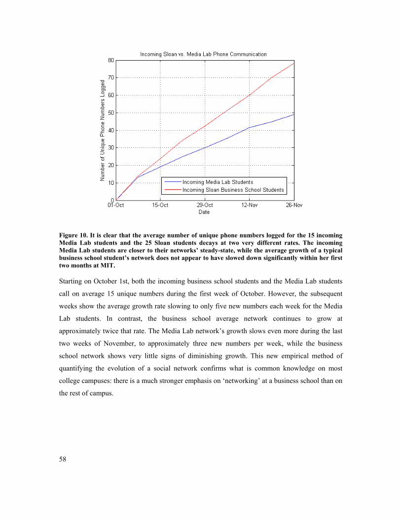
58

Figure 10. It is clear that the average number of unique phone numbers logged for the 15 incoming Media Lab students and the 25 Sloan students decays at two very different rates. The incoming Media Lab students are closer to their networks’ steady-state, while the average growth of a typical business school student’s network does not appear to have slowed down significantly within her first two months at MIT.

Starting on October 1st, both the incoming business school students and the Media Lab students

call on average 15 unique numbers during the first week of October. However, the subsequent

weeks show the average growth rate slowing to only five new numbers each week for the Media

Lab students. In contrast, the business school average network continues to grow at

approximately twice that rate. The Media Lab network’s growth slows even more during the last

two weeks of November, to approximately three new numbers per week, while the business

school network shows very little signs of diminishing growth. This new empirical method of

quantifying the evolution of a social network confirms what is common knowledge on most

college campuses: there is a much stronger emphasis on ‘networking’ at a business school than on

the rest of campus.

59

4.5 Sampling Dynamic Networks

The topology of complex networks, such as that of social and technological networks, is often a

dynamic property with edges and vertices appearing and disappearing in time. Most

characterizations of them, however, assume the topology is fixed in time, or, at best, the changes

are aggregated into a discrete sequence of adjacencies where network parameters are measured as

a function of time. Using an empirical network with high-resolution temporal data, we show that

the size of the sampling interval ∆ determines the value of the measured network parameters. We

then show that spectral analysis can uncover the natural harmonics of topological dynamics and

indicate the correct sampling rate, which we then use to measure several topological statistics of

our network.

4.5.1 Overview

Complex systems of interacting components can often be represented as a network, i.e., n nodes

or vertices joined together in pairs by m links or edges, and the analysis of the resulting

topological structure [Newman (2003), Albert & Barabási (2002), Dorogovtsev & Mendes

(2002)] can yield significant insights into the original system. Recently, systems from a wide

variety of domains, including social [Newman & Park (2003), Scott (2000), Watts & Strogatz

(1998)], technological [Clauset & Moore (2005), Jeong & Barabási (1999), Kleinberg &

Lawrence (2001)] and biological [Shen-Orr et al. (2002), Williams & Martinex (2000), Jeong et

al. (2000)] systems, have been formulated as networks. Two of the most commonly measured and

best studied topological features of networks are the degree distribution, i.e., the probability

( )P k that a randomly selected vertex will have k neighbors, and the clustering coefficient C ,

i.e., the probability that two neighbors y , z of a vertex x will themselves be neighbors. It is

now well documented that many real world networks have highly right-skewed degree

distributions, either exponential ( ) e kP k α−∼ or power-law ( )P k k α−∼ distributions where α is

some constant, and large clustering coefficients, with typical values being 0 1 0 5C. ≤ ≤ . , relative

to a purely random graph.

However, for many networks, the topology is not a static property: both the number of edges and

vertices fluctuate in time. Traditionally, network analysis deals with this variability in one of the

60

following ways: 1) assume that the topology is effectively static, i.e., network structure can be

sampled quickly relative to the speed of the fluctuations, 2) assume that any fluctuations at most

add a small amount of unbiased noise to any measurements, or 3) incorporate the fluctuations into

the analysis by measuring topological features over a sequence of network “snapshots” in which

the interactions are aggregated over sequential periods of length ∆ (where ∆ might be very

small). Generally, this latter approach is the most common one used for the analysis of explicitly

dynamic topologies and has been used to characterize the evolution of a Brazilian soccer

network [Onody & de Castro (2004)], an email exchange, scientific collaboration, and online

dating networks [Holme (2003)], the student affiliation network of a Korean university [Holme et

al. (2004)], as well as the Internet, a co-authorship network and a semantic network [Vazquez et

al. (2005)].

In this section, we address the question of how to analyze the structure of a network with a

dynamic topology. In particular, we characterize the effect of the sampling interval ∆ on the

measured topological parameters, such as degree statistics, the correlation coefficient, and a

topology similarity measure that we introduce. We show choosing a sampling interval ∆

determines the measured network statistics. Additionally, we show that spectral methods can help

us to uncover known natural periodicity in the network dynamics and select an appropriate ∆ by

which to characterize the network’s structure. Finally, we briefly comment on the significance of

our results to other dynamic network studies, and on the implications for future studies as more

dynamic network data become available.

4.5.2 Network Metrics

In this section, we briefly review existing and commonly used network metrics for static

topologies and their extension to network sequences. We also introduce a similar metric for

characterizing the extent of correlation between the topologies of two networks.

Traditional Methods. Networks are often represented as an adjacency matrix A , which is

defined as

1 if vertices and are connected0 otherwisei j

i jA ,

,= .

61

From this, one can calculate the degree of each vertex i by taking the corresponding row (or

column) sum. The distribution of these degrees ( )P k is a ubiquitous first-order representation of

the network’s topological structure. It is notable that the value of the mean degree k is closely

connected with the concept of the excess, which is the number of additional edges in the network

beyond that required to ensure that a path exists between any two vertices. Adjacency matrices

are generalizable to weighted graphs, and the row (column) sum then becomes the strength of the

vertex, with ( )P w the distribution of strengths.

The clustering coefficient C is a measure of the density of triangles in the graph, and represents

the probability that two vertices that have a common neighbor will themselves be neighbors. The

clustering coefficient is given as

1

1 (number of triangles centered on vertex )(number of triples centered on vertex )

n

i

iCn i=

= .∑ 4-1

where n is the number of vertices in the network. Most real world networks exhibit large

clustering coefficients relative to random graphs [Erdős & Rényi (1960)]. Note that a large

average degree k does not necessarily imply a large clustering coefficient, although it may, when

1k n/ ∼ . The clustering coefficient can be generalized to weighted graphs [Barthélemy et al.

(2005)].

Adjacency Correlation. Here, we propose a similarity measure of a vertex’s connectivity at one

moment and another, which we call the adjacency correlation γ . Given a pair of adjacency

matrices 1( )tA and 2( )tA at times 1t and 2t , the similarity of the connectivity for a vertex j

between these two moments is simply the correlation between the adjacency vectors for j .

However, when the graph is sparse, i.e., m n∼ , as is the case for most real world graphs of

interest, most entries in both vectors will remain constant regardless of dynamics. Thus, without

loss of generality, we may compute the correlation calculation simply over those elements that

correspond to neighbors that j connects to in either of the matrices. We denote this set as ( )N j ,

and the adjacency correlation for j to be

62

( ) ( )1 2

1 2

( ) ( )( )

( ) ( )( ) ( )

t ti j i ji N j

jt t

i j i ji N j i N j

A A

A Aγ , ,∈

, ,∈ ∈

=∑

∑ ∑. 4-2

When the adjacency vectors contain no edges, the adjacency correlation is undefined, so for

convenience, we take 1jγ = in this case. We can easily generalize this metric to a sequence

adjacency matrices ( )tA , with 1 2t … T= , , , , where we take ( )N j to be the set of unique

neighbors over all of these matrices. Averaging the adjacency correlation over all vertices yields

the desired measure of topology similarity. Note that the adjacency correlation need not

necessarily be computed between adjacent moments of time t and 1t + , although this is the

convention we adopt throughout this work, nor is it restricted to only unweighted or undirected

networks.

4.5.3 Sampling Dynamic Networks

We now turn to the question of what impact sampling a changing topology has on the structural

measures described in the previous section. As has been convention with studying dynamic

networks, unless otherwise noted, we use the unweighted versions of the metrics. After

demonstrating that the topology of our exemplar dynamic network evolves on a wide variety of

time-scales, we will show that the sampling rate directly determines the calculated topological

properties of the network’s structure.

Sampled Topology. We now generalize the concept of sampling the topology of a dynamic

network, and turn to the question of what effect varying the length of the sampling interval ∆ has

on inferred topological parameters. Given a network with underlying continuous dynamics, in

which edges have both an initiation and termination time, we define the sampled adjacency

matrix ( )tB , which represents the network at moment t , to be

( )

1 if vertices and are ever connectedbetween time and

0 otherwise

ti j

i jB t t,

= + ∆, .

63

This process produces a discrete sequence of T matrices, where 0 0 0 ( 1)t t t … t T= , + ∆, , + − ∆ .

Conceptually, this definition is not unlike a series of time-lapse photographs, where within a

snapshot, multiple transient interactions are seen as a single prolonged interaction; this is akin to

classic under-sampling, and may introduce artificial structure when the sampling period is longer

than the time-scale of the topological dynamics. It is often the case for empirical studies of

dynamic networks that T and ∆ are constrained by the availability of data, the assumption of a

lower bound on the time scale of interactions, or a desire to ensure that a large fraction of vertices

are connected, i.e., a giant component exists.

Figure 11. The (a) mean degree k , (b) mean clustering coefficient C and (c) complementary network adjacency correlation 1 γ− as a function of time for ∆ =1440, 480, 240, 60, 15, 5 (minutes) during the week of 11 October through 17 October for the core 66 subjects. As ∆ grows, under-sampling clearly washes out higher frequency fluctuations.

Sampling Effects. From the high temporal resolution of the dynamic proximity network we may

simulate a near arbitrary choice of ∆ and T , and thus explore the effects of sampling. Using the

intervals 1440 480 240 60 15 5∆ = , , , , , minutes, we compute the mean degree k (Figure 11a),

the clustering coefficient C (Figure 11b), and the complementary network adjacency correlation

1 γ− (Figure 11c) for each adjacency matrix ( )tB over the course of seven days beginning with

11 October. The shortest sampling interval, 5∆ = minutes, exhibits high frequency noise

combined with low frequency structure; this latter arises from the subjects’ professional co-

location. As expected for sampling below the Nyquist rate, as ∆ increases, progressively lower

frequency fluctuations are lost. Indeed, when 1440∆ = minutes (1 day), most days appear

equivalent within a metric, with slight differences emerging on the weekend. This regularity

remains consistent over longer period of time; larger sampling intervals do not accurately reflect

the fact that the topology evolves at a variety of time-scales and that interactions during a given

64

interval are often more typically recurrent than persistent. We attain similar periodic behavior for

the weighted versions of these metrics; however, without loss of generality, we will discuss only

the unweighted results in the subsequent sections.

In Figure 12, we show the measured values of each metric averaged over the entire month of

October as a function of ∆ . The roughly monotonic growth of each illustrates that a choice of

sampling interval completely determines the resulting observed metric value.

Figure 12. The values of each network metric (mean degree k n/ , mean clustering coefficient C and mean complementary adjacency correlation 1 γ− ) during the month of October as a function of aggregation interval ∆ ; clearly, the value of each metric is proportional to the choice of ∆ .

65

Figure 13. The power spectra of three metric time series at 5∆ = minutes over the course of the month of October. The principal peaks are at 24 12∆ = , hours, with additional minor peaks at

8∆ = hours for the mean degree and clustering coefficient.

Discussion. Representing a complex system as a network has been a powerful analytical

paradigm. To date, much of the work done has been on static networks such as biochemical

pathways, predator-prey relationships, and collaboration networks, in which edges are forever

fixed rather than dynamic connections. However, there is great potential benefit in similarly

representing and analyzing inherently dynamic systems such as proximity, social, genetic

expression, and cell signaling networks. In representing these systems, we can only sample their

topology over time; however, until now, there has been no principled study of how such sampling

impacts the statistical results of network analysis. Additionally, there is a dearth of useful tools

for such analysis. Towards improving this latter point, here we introduce a similarity statistic for

comparing the topology of networks at different moments in time, which we call the adjacency

correlation coefficient and denote as γ .

In exploring the effects of the rate of sampling on the observed topology, we demonstrate that

when a network’s structure changes over a broad range of time-scales, the inferred statistics are

66

completely determined by the choice of sampling rate. This determinism is the result of the

largely monotonic increase in the network density k n/ with the length of the sampling interval

∆ ; this result is extremely problematic for a dynamic network because it is not clear which of the

values naturally characterizes the system. To resolve this problem, we show that spectral analysis

techniques can characterize the network dynamics’ natural harmonics. This approach puts

dynamic networks on familiar ground in the company of well-established tools. Additionally, the

concept of dynamic networks having natural harmonics is novel; many previous characterizations

have focused on networks that grow over time rather than on those that appear to be in a dynamic

equilibrium.

In addition to our results on sampling dynamic networks and their harmonic characterization, we

make several comments on the measured properties of dynamic proximity networks. The

broadness of the measured distribution of the persistence of edges is notable; however, it is

clearly not so broad as to be a power law, as is often found in human systems [Newman (2005)].

We look forward to additional high resolution dynamic network data becoming available so as to

determine if such a broad distribution is a ubiquitous feature of real dynamic complex networks.

Although it is true for our dynamic proximity network, the harmonics of various networks

statistics may not be synchronized in other dynamic networks; indeed, asynchronous behavior

may be suggestive of non-equilibrium forces, while synchronous behavior suggests driving forces

such as the period of the day and week, or perhaps self-organizing dynamics. Further work is

needed to answer these and other questions.

67

Chapter 5 Illustrative Models and Applications

In this chapter we will discuss how the data we are collecting can be modeled and applied to

complex human networks on a variety of scales ranging from the single individual to the

aggregate organization. We initially introduce the idea of entropy, or randomness, as a metric that

can be quantified for an individual’s life. The more entropic a subject’s life, the harder it is to

model and predict subsequent behavior. While additional models based on eigendecomposition

are introduced in a subsequent chapter, we introduce the conditioned hidden Markov model in

this chapter as a method of defining a user’s behavior. We then discuss two applications of this

data for the individual: an automatically generated diary and a system for recognizing the gist of a

user’s conversation using contextual information gathered from the phone. Secondly, we turn our

attention to dyads and show that it is possible to infer relationships between subjects based on

patterns in proximity data. Quantifying the dynamics of teams and organizations becomes the last

subject of this chapter. We compare the patterns of two teams within the Media Lab and show

how the lab as an aggregate responds to stimuli such as deadlines.

5.1 Individual Modeling and Applications

Although humans have the potential for relatively random patterns of behavior, there are easily

identifiable routines in every person’s life. These can be found on a range of timescales: from the

daily routines of getting out of bed, eating lunch, and driving home from work, to weekly patterns

such as the Saturday afternoon softball games, to yearly patterns like seeing family during the

holidays in December. While our ultimate goal is to create a predictive classifier that can perceive

aspects of a user’s life more accurately than a human observer (including the actual user), we

begin by building simple mechanisms that can recognize many of the common structures in the

user’s routine. Learning the structure of an individual’s routine has already been demonstrated

using other modalities; however, we present this analysis as a foundation which will then be

extended to demonstrate the learning of social structures.

We begin with a simple model of behavior in three states: home, work, and elsewhere. The data

are obtained from Bluetooth, cell tower, and temporal information collected from the phones. We

then incorporate information from static Bluetooth devices (class 1, such as desktop computers),

68

using them as ‘cell towers’ to identify significant locations and localize the user to a ten meter

radius. We show that most users spend a significant amount of time in the presence of static

Bluetooth devices, particularly when they don’t have cell tower reception (e.g., inside the office

building). This makes them an ideal supplement to cell towers for location classification.

Applications that make use of this recognized structure include a diary that enables users to make

limited queries into their own logged experiences, i.e., “When was the last time I saw Josh?

Where was I? Who else was there?” Additionally, using a database of first-person commonsense

propositions about daily life called LifeNet, we show it is possible to use contextual information

from the phone to augment noisy speech recognition transcripts. For example, by conditioning on

the fact that the user is in a restaurant with a friend, it is much easier to make sense of a

conversation transcript that has only a 33% word recognition accuracy.

5.1.1 The Entropy of Life

Human life is inherently imbued with routine across all temporal scales, from minute-to-minute

actions to monthly or yearly patterns. Many of these patterns in behavior are easy to recognize;

however, some are more subtle. We attempt to quantify the amount of predictable structure in an

individual’s life using an information entropy metric. In information theory, the amount of

randomness in a signal corresponds to its entropy, as defined by Claude Shannon in his 1938

master’s thesis at MIT in the equation below.

21

( ) ( ) log ( )n

iH x p i p i

=

= −∑ 5-1

For a more concrete example, consider the problem of image compression (such as the jpeg

standard) of an overhead photo taken of just an empty checkerboard. This image (in theory) can

be significantly compressed because it does not contain much ‘information.’ Essentially the entire

image could be recreated with the same, simple pattern. However, if the picture was taken during

the middle of a match, the pieces on the board introduce more randomness into image, and

therefore, it will prove to be a larger file because it contains more information, or entropy.

Similarly, people who live entropic lives tend to be more variable and harder to predict, whereas

low-entropy lives are characterized by strong patterns across all time scales. Figure 14 depicts the

69

patterns in cell tower transitions and the total number of Bluetooth devices encountered each hour

during the month of January for Subject 9, a ‘low entropy’ subject.

Figure 14. A ‘low-entropy’ (H = 30.9) subject’s daily distribution of home/work transitions and Bluetooth devices encounters during the month of January. The top figure shows the most likely location of the subject: “Work, Home, Elsewhere, and No Signal.” While the subject’s state sporadically jumps to “No Signal,” the other states occur with very regular frequency. This is confirmed by the Bluetooth encounters plotted below representing the structured working schedule of the ‘low-entropy’ subject.

It is clear that the subject is typically at home during the evening and night until 8:00, when he

commutes to work, and then stays at work until 17:00 when he returns home. We can see that

almost all of the Bluetooth devices are detected during these regular office hours, Monday

through Friday. This is certainly not the case for many of the subjects. Figure 15 displays a

different set of behaviors for Subject 8. The subject has much fewer regular patterns of location

and in the evenings has other mobile devices in close proximity. We will use contextualized

information about proximity with other mobile devices to infer relationships, described in section

5.2.2.

70

Figure 15. A ‘high entropy’ (H = 48.5) subject’s daily distribution of home/work transitions and Bluetooth device encounters during the month of January. In contrast to Figure 14, the lack of readily apparently routine and structure makes this subject’s behavior harder to model and predict.

While calculating life’s entropy can be used as a method of self-reflection on the routines (or ruts)

in one’s life, it can also be used to compare the behaviors of different demographics. Figure 16

shows the average weekly entropy of each of the demographics in our study, based on her

location work, home, no signal, elsewhere each hour. Average weekly entropy was calculated

by drawing 100 samples of a 7-day period for each subject in the study. No surprise to most, the

Media Lab freshman undergraduates are the most entropic of the group. The freshmen do not

come into the lab on a regular basis and have seemingly random behavior with ( ) 47.3H x =

(the entropy of a sequence of 168 random numbers is approximately 60). The graduate students

(Media Lab incoming, Media Lab senior, and Sloan incoming) are next most entropic with

( ) 44.5, 42.8, 37.6H x = respectively. Finally, the Media Lab faculty and staff have most

rigidity in their schedules, reflected in their relatively low average entropy measures,

( ) 31.8, 29.1H x = .

71

Figure 16. Entropy, H(x), was calculated from the work, home, no signal, elsewhere set of behaviors for 100 samples of a 7-day period. The Media Lab freshmen have the least predictable schedules, which makes sense because they come to the lab on a much less regular basis. The staff and faculty have the most least entropic schedules, typically adhering to a consistent work routine.

One similarity between the different demographics shown above is the clear role time plays in

determining user behavior. To account for this, we have developed a simple Hidden Markov

Model conditioned on both the hour of day ( 1 1, 2,3..., 24T ∈ ) as well as weekday or weekend

( 2 1, 2T ∈ ). Observations in the model initially are simply the distribution of cell towers

( 1

11 1, ,..., nY CT CT CT∈ ) and Bluetooth devices ( 2

21 1, ,..., nY BT BT BT∈ ). A straightforward

Expectation-Maximization inference engine was used to learn the parameters in the transition

model, ( )1|t tP Q Q − , and the observation model ( )|t tP Y Q , and performed clustering in which

we defined the dimensionality of the state space. The hidden state is represented in terms of a

single discrete random variable corresponding to three different situations,

, , Q home work other∈ . After training our model with one month of data from several

subjects we were able to provide a good separation of clusters, typically with greater than 95%

accuracy. Examination of the data shows that non-linear techniques will be required to obtain

72

significantly higher accuracy. However, for the purposes of this chapter, this accuracy has

proven sufficient.

Figure 17. A Hidden Markov Model conditioned on time for situation identification. The model was designed to be able to incorporate many additional observation vectors such as friends nearby, traveling, sleeping, and talking on the phone.

5.1.2 Life Log

The last several years have seen search engine companies such as Google, MSN Search, and

Yahoo reinvent themselves from companies that simply perform optimized queries on cached

web content, to multimedia search engines for all types of content including images, email, and

even files on users’ personal computers. With Google’s recent acquisition of Blogger, Yahoo’s

Blog Directories, and MSN Spaces, it is clear that logging and mining the content from users’

blogs (web diaries) has become a major priority for search industry. However, while many

‘bloggers’ relish the opportunity to transcribe and publish the minutia of their lives, most people

don’t take the time to write such diaries.

Nevertheless, simply because most people do not want to spend time manually logging daily

experiences does not imply that the logs themselves are undesired. In 1945, Vannevar Bush laid

out his vision for the “memex” [Bush (1945)], a device that records every detail of human

memory and facilitates simple search and retrieval of experiences. While technically infeasible in

his era, with the advent of wearable sensors and large amounts of disk space, many researchers

today have begun pursuing their own version of the memex [Clarkson (2002), Vemuri (2004),

Gemmell (2005)].

73

In collaboration with Mike Lambert, we have created an interactive, automatically generated

diary application that enables users to query their own life (i.e., “When was the last time I went

out on the town with Mike? Where were we? Who else was there? When did I get home?”) .

Labels for locations can be input by the user through the web interface but are also learned from

the phone application itself. If a user spends a significant amount of time in a specific tower, the

phone vibrates and prompts the user to name the location or situation. Examples of user input

names include “Media Lab, My Dorm, Mike’s Apartment, Club Downtown, etc.”

The original system was Flash-based with a LISP server backend and processed raw text logs

from the phones. The client was written in ActionScript, which limited the scalability and

interaction potential of the application. The current version of LifeLog has been redesigned in

Java to provide much faster load times and easier navigation [Lambert (2005)] and is shown

below.

74

Figure 18. LifeLog - automatic diary generation. LifeLog provides a visualization of the data from the Reality Mining phone logs and inferences. It has also incorporated the ability to perform “life queries,” allowing the user to search through previous events and experiences.

5.1.3 Conversation Gisting from Context and Common Sense

Conditioning on the location and situation information discussed above, it is possible to get a

much better interpretation of other types of data gathered from the user. In collaboration with

Push Singh, we have combined this contextual information from the phone with noisy speech

recognition transcripts, and a database of commonsense information called OMCSNet, in an

effort capture the ‘gist’ or topic of a subject’s conversation. While traditional speech-recognition

rates for conversational speech are typically well under 40%, by conditioning the inference with

knowledge that the conversation is taking place in a restaurant and some commonsense facts

75

about what typically goes on in restaurants, we will show that it is possible to extract the topics of

many conversations.

5.1.3.1 Common Sense Reasoning

For many applications, it can be quite valuable to combine sensor data on human behavior with

higher-level, propositional knowledge about day-to-day problems and work patterns. We have

found that this task can be greatly aided by using commonsense knowledge [Singh (2002)]. For

instance, by combining information from the audio stream and from other available contextual

cues with commonsense knowledge about the activities people engage in and the topics they care

about, we can infer a clearer picture of the content of conversations and the context of their

participants [Eagle et al. (2003), Lieberman & Liu (2002)].

We make use of OMCSNet, a large-scale semantic network built at the Media Lab by aggregating

and normalizing the contributions from over 10,000 people from across the web [Singh (2002)]. It

presently consists of over 250,000 commonsensical semantic relationships of the form ‘a printer

is often found in an office,’ ‘going to a movie requires buying a ticket,’ and so forth. OMCSNet

contains a wide variety of knowledge about many aspects of everyday life: typical objects and

their properties, the effects of ordinary actions, the kinds of things people like and dislike, the

structure of typical activities and events, and many other things. OMCSNet uses a hybrid

knowledge representation strategy where individual concepts are represented linguistically

(lexically and phrasally) and are related by a small set of about twenty specific semantic

relationships such as LocationOf, SubeventOf, HasEffect, and so on.

Our system’s goal is to infer the ‘fine grained topic,’ or gist, of the conversation. A gist is the

class of event that most accurately summarizes the current subject of the conversation. For

example: buying a ticket to a baseball game, looking for a restaurant, scheduling a meeting, and

canceling a meeting. These gists are represented within OMCSNet as simple verb phrases. For

our set of target gists, we use the 700 most richly defined situational aspects within OMCSNet

(those for which at least 10 facts are asserted). One feature that distinguishes commonsense

reasoning from other forms of reasoning is that it involves making inferences using many

different kinds of knowledge: about objects, events, goals, locations, and so forth. Accordingly,

76

our system uses a probabilistic model that incorporates different types of knowledge, as well as

contextual data from the mobile phones.

5.1.3.2 Inference in OMCSNet

Inference over the OMCS network can be done with varying levels of complexity, ranging from

simple network analysis metrics to probabilistic modeling using Bayesian networks. Before the

inference, the transcriptions are preprocessed to reduce the noise of the speech recognition engine

and improve inference performance. The transcriptions are first lemmatized and filtered for stop

words (such as ‘like,’ ‘the,’ ‘a,’ etc.). A second filtering process is then performed using a

clustering metric to reduce the number of weakly connected words. These outliers, words with

very sparse links to the rest of the transcription, are removed from the data set. By flattening the

networks of the different relationship types, a bipartite network can be formed to incorporate all

ties from words to gists. The probability of a specific gist can be modeled as proportional to the

gist’s links to the selected words:

1

( ) ii G

i

i

kP g kk

=

∝∑

5-2

where ik is the number of links between a gist, ig , and the observed transcript, and G is the

number of potential gists (approximately 700). This method is capable of identifying a small

group of potential gists, frequently with the ‘correct’ one dominating the others.

Once the probable topics of conversation have been identified and ranked, contextual information

about the conversation is incorporated into the model. In many instances, information such as

location or participant identity can identify the gist from the small subsection of topics. In our

initial tests we incremented a gist’s score for each of its links to a keyword related to the given

context.

5.1.3.3 Experiments

We ran a series of 20 interaction experiments on speech segments ranging from 50 to 150 words

covering a wide range of topics. Conversational context was limited to location. Using the

method described above, a ranking of the top ten gists for each interaction was created. The

77

model gave a correct gist the number 1 ranking in 40% of the tests. In 70% of the tests, a correct

gist was one of the top-ranking three. However in 25% of the tests, a correct gist was ranked

outside the top ten.

As an example to illustrate the functioning of the system, in one test we captured conversations

from the student center cafeteria mapped as ‘restaurant.’ Using words alone produced a useful

result, but using words along with the contextual information to condition the model greatly

improved our results:

Actual situation: Deciding what to get for lunch in the cafeteria.

Automatic transcription: Store going to stop and listen to type of its cellular and fries he backed a bill in the one everyone get a guess but that some of the past like a salad bar and some offense militias cambers the site fast food them and the styrofoam large chicken nuggets son is a pretty pleased even guess I as long as can’t you don’t have to wait too long its complicity sunrise against NAFTA pact if for lunch.

Automatically selected keywords: Wait type store stop salad past lunch long long listen large fry food fast chicken cellular bill big bar back

Without Location Context With Location Context 5 talk with someone far away 27 eat in fast food restaurant 5 buy beer 21 eat in restaurant 5 Eat in restaurant 18 wait on table 5 eat in fast food restaurant 16 you would go to restaurant because you 5 buy hamburger 16 wait table 4 go to hairdresser 16 go to restaurant 4 wait in line

15 know how much you owe restaurant

4 howl with laughter 12 store food for people to purchase 4 eat healthily

11 sitting down while place order at bar

4 4 play harp 11 cook food

Table 5 Gist classification with and without location information from the phone; the numerical score is the number of links to the gist. By biasing the classifier with the fact that the subject is in a restaurant, it becomes much easier to infer the topic of conversation from noisy transcripts.

5.2 Dyadic Inference

In the previous section we have showed how information regarding a user’s location can be used

for an automatic diary system or to generate better inferences about conversation topic. In this

section we will explore the possibilities associated with logging not only information about a

user’s physical environment, but also the surrounding social environment. As discussed

previously, repeated Bluetooth scans of the vicinity provide information about the subjects within

ten meters of the user. We will show that this information can be used to establish ‘human

78

landmarks,’ people who are strongly correlated with a particular location. When this proximity

information is also coupled with temporal and contextual information, it becomes possible to

infer relationship between members of a given dyad.

5.2.1 Human Landmarks

As shown in Figure 6 and Figure 20, there are people whom users only see in a specific context

(in this instance, at work). If we know the user is at work, information about the time of day, and

optionally the location within the building (using static Bluetooth devices), can be used to

calculate the probability of that user seeing a specific individual by the straightforward

application of Bayes’ rule.

In previous work in the Computer Supported Cooperative Work (CSCW) community, there has

been an emphasis on mobile calendar applications that access everyone’s calendar and can

suggest appropriate times to schedule a meeting scheduling [Beard et al. (1990), Roth and Unger

(2000)]. In contrast to this work that relies on each user keeping his or her calendar up-to-date,

we can generate inferences about whether a person will be seen within the hour, given the user’s

current context, with accuracies of up to 90% for ‘low entropy’ subjects. These predictions can

inform the user of the most likely time and place to find specific colleagues or friends. We

believe that the ability to instigate casual meetings would be of significant value in the workplace.

We must also remember, however, that the ability to predict people’s movements can be put to

less savory uses. Careful consideration must be given to these possibilities before providing free

access to such data.

5.2.2 Relationship Inference

In the first part of this chapter, we discussed how information about location and proximity can

be used to infer a user’s context. In much the same way, knowledge of the shared context of two

users can provide insight into the nature of their association. For example, being near someone at

3pm by the coffee machines confers different meaning than being near her at 11pm at a local bar.

However, even simple proximity patterns provide an indication of the structure of the underlying

friendship network, as shown in Figure 19. The clique on the top right of each network are the

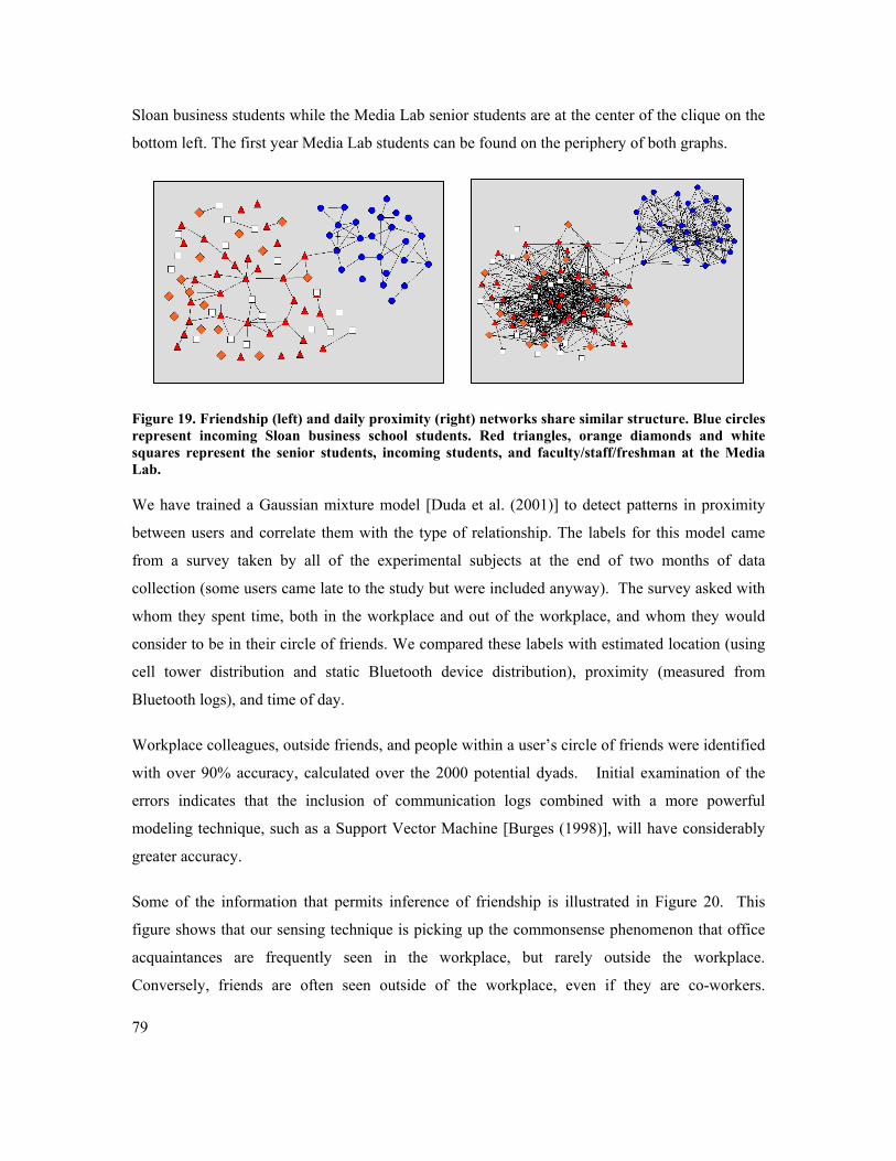
79

Sloan business students while the Media Lab senior students are at the center of the clique on the

bottom left. The first year Media Lab students can be found on the periphery of both graphs.

Figure 19. Friendship (left) and daily proximity (right) networks share similar structure. Blue circles represent incoming Sloan business school students. Red triangles, orange diamonds and white squares represent the senior students, incoming students, and faculty/staff/freshman at the Media Lab.

We have trained a Gaussian mixture model [Duda et al. (2001)] to detect patterns in proximity

between users and correlate them with the type of relationship. The labels for this model came

from a survey taken by all of the experimental subjects at the end of two months of data

collection (some users came late to the study but were included anyway). The survey asked with

whom they spent time, both in the workplace and out of the workplace, and whom they would

consider to be in their circle of friends. We compared these labels with estimated location (using

cell tower distribution and static Bluetooth device distribution), proximity (measured from

Bluetooth logs), and time of day.

Workplace colleagues, outside friends, and people within a user’s circle of friends were identified

with over 90% accuracy, calculated over the 2000 potential dyads. Initial examination of the

errors indicates that the inclusion of communication logs combined with a more powerful

modeling technique, such as a Support Vector Machine [Burges (1998)], will have considerably

greater accuracy.

Some of the information that permits inference of friendship is illustrated in Figure 20. This

figure shows that our sensing technique is picking up the commonsense phenomenon that office

acquaintances are frequently seen in the workplace, but rarely outside the workplace.

Conversely, friends are often seen outside of the workplace, even if they are co-workers.

80

Determining membership in the ‘circle of friends’ requires cross-referencing between friends: is

this person a member of a cluster in the out-of-office proximity data?

Figure 20. Proximity frequency data for a friend and a workplace acquaintance. The top two plots are the times (time of day and day of the week, respectively) when this particular subject encounters another subject he has labeled as a “friend”. Similarly, the subsequent two plots show the same information for another individual the subject has labeled as “office acquaintance.” It is clear that while the office acquaintance may be encountered more often, the distribution is limited to weekdays during typical working hours. In contrast, the subject encounters his friend during the workday, but also in the evening and on weekends.

81

Friends Not Friends

avg std avg std

Total Proximity (minutes / day)

72 150 9.5 36

Saturday Night Proximity (minutes /

week)

7.3 18 .20 1.7

Proximity with no Signal (minutes / day)

12 20 2.9 20

Total Number of Towers Together

20 36 3.5 4.4

Proximity at Home (minutes / day)

3.7 8.4 .32 2.2

Phone Calls / day .11 .27 .001 .017

Table 6. Statistics correlated (.25<R<.8, p<.001) with friendship generated from sixty subjects (comprising 75 friendships) who work together at the Media Lab

5.3 Modeling Teams & Organizations

By continually logging and time-stamping information about many collated individuals’ activity,

location, and proximity to other users, the large-scale dynamics of collective human behavior can

be analyzed. Furthermore, a dataset providing the proximity patterns and relationships within

large groups of people has implications within the computational epidemiology communities, and

may help build more accurate models of airborne pathogen dissemination, as well as other more

innocuous contagions, such as the flow of information.

In the previous section we showed that Bluetooth-enabled mobile phones can be used to discover

a great deal about the user’s context and relationships. In this section we will extend this base of

user modeling to explore modeling complex social systems. We will provide several illustrative

examples how this data can be used to learn more about both team and organizational dynamics.

82

5.3.1 Team Dynamics

By continuously logging the people proximate to an individual, we are able to quantify a variety

of properties about the individual’s work group. Although most research in networks assumes a

static topology, proximity network data is extremely dynamic and sparse. While we go into in-

depth analysis of the dynamics of these networks in Chapter 4, in this section we will compare

aggregate statistics between two different research groups at the Media Lab in an attempt to gain

insight into fundamental characteristics of the research groups themselves.

Figure 21. Proximity network snapshots for a research group over the course of one day. In this example, if two of the group members are proximate to each other during a one-hour window, an edge is drawn between them. The four plots represent four of these one-hour windows throughout the day at 10:00, 13:00, 17:00, and 19:00. We have the ability to generate these network snapshots at any granularity, with windows ranging from five minutes to three months.

83

Figure 22. Proximity Network Degree distributions between two groups. The left-most plot corresponds to the Human Dynamics group’s degree distribution (i.e., the number of group members each person is proximate to over an aggregate of network snapshots). The second left-most plot is simply zoomed-in on the tail of the previous plot’s distribution. Likewise, the two right-most plots are of the Responsive Environments group’s degree distribution.

In Chapter 4, we showed data indicating that a subject’s satisfaction with his research group is

closely tied to the number of friendship ties he has within the group. However, literature on

teams also emphasizes the fact that not only does the number of ties among teammates matter, but

also the pattern of those ties is important. Starting with the groundbreaking experiments in the

1950’s and 1960’s by Bavelas, Leavitt and colleagues at the Group Networks Laboratory at MIT

[Leavitt (1951)], researchers have focused on the issue of centralization: the extent to which ties

form a hub-and-spoke pattern, with one team member serving as the central sender and recipient

of messages. The research suggests that the benefits of centralization depend upon the nature of

the task. When the task is complex, teams with decentralized communication patterns outperform

teams with centralized communication patterns [Cummings & Cross (2003), Sparrowe et al.

(2001)]. What conditions promote the emergence of a centralized pattern of ties? Two

experimental studies have addressed this question and found that a centralized pattern is more

likely to arise on teams assigned to relatively high stress conditions [Argote et al. (1989)] or

relatively low complexity tasks [Brown & Miller (2000)].

While each research group at the Media Lab is centralized around a faculty director, the

proximity networks are not reflective of this static organizational structure. In many instances, the

proximity network’s degree distribution is indicative of a hub-and-spoke formation; however, the

84

roles that are played within this structure are not static. Individuals that are hubs during one

period of time fluidly exchange places with other team members on the periphery of the

proximity network. This type of dynamic may be characteristic of the underlying nature of

research groups at the Media Lab. As deadlines approach for specific individuals, they begin to

spend more time in the Media Lab and increasingly rely on support from the rest of the group.

Upon completion of a project, they resume their normal routines and can provide similar support

to others. As will be discussed in the next section, this pattern of behavior has been shown to

vanish when the entire group (or organization) is working towards the same deadline.

5.3.2 Organizational Modeling & Rhythms

Organizations have been considered microcosms of society, each with its own culture and values

[Wertheim (2003)]. Similar to society, organizational behavior often shows recurrent patterns

despite being the sum of the idiosyncratic behavior of individuals [Begole et al. (2003)]. In this

section we explore the ramifications of the ability to quantify the dynamics of behavior in

organizations in response to both external (stock market performance, a Red Sox World Series

victory) and internal (deadlines, reorganization) stimuli.

5.3.2.1 The Need for Better Organizational Models

Over time, the Reality Mining data can be fine-tuned for studying, tracking, and - perhaps most

importantly - predicting the dynamics of a particular social network. Recently, the CEO of a

multimillion-dollar manufacturing company became interested in the technology as a means to

quantify workplace collaboration. Like many organizations, his company suffers from the “silo

syndrome”, ie: people from different departments tend to keep to themselves, leading to

inefficiencies and missed opportunities.

To address that problem, the CEO had tried a number of initiatives, for example, having dozens

of people from marketing switch offices with their counterparts in engineering; however, he

realized that he did not have a clear understanding about how those changes actually affected the

organization as a whole. The company had conducted extensive surveys, but the data only

provided a snapshot of the current social network. Instead, the CEO said he wanted “footprints in

the sand” to understand the dynamics of the network topology. With such information, he could

then determine signature effects indicative of a successful (or unsuccessful) initiative.

85

Augmenting his existing data collection methods with data from unobtrusive mobile phones could

help capture exactly those types of continuous dynamics.

5.3.2.2 Organizational Rhythms: Patterns in Aggregate Behavior

From the proximity data, we first extract adjacencies for each scan and then infer ongoing

proximity so as to annotate each edge with an initiation and termination time. At the time of

writing, we are not aware of any other network data set with such a large amount of temporal data

or one with such fine granularity. Thus, this data set provides a rich opportunity to explore both

temporal dynamics and the quality of our analytic tools. Here we focus on the latter.

Broad-Scaled Dynamics Given the initiation and termination times of each edge, the difference

gives the edge’s temporal persistence. Here we restrict our analysis to the 24,092 undirected

subject-subject adjacencies between 01 October 2004 and 31 October 2004 of the 66 subjects

who work in the same building at MIT. Figure 23 illustrates the inverse cumulative persistence

distribution ( )P x X> (in minutes) for both two weeks within and the full month of October.

Unsurprisingly, the weekly and monthly distributions are largely similar, with minor variations

far out in the tail, i.e., for persistence greater than 400 minutes, suggesting a system largely in

equilibrium. The typical duration of proximity is relatively small, being only 22 83. minutes,

while there are several (three) edges which persist for more than 1440 minutes (24 hours). The

broadness of these distributions demonstrates that the network’s topology evolves at a wide

variety of time-scales, and we believe such a distribution may be typical of many real world

networks. Indeed, although not well-motivated for our data set, a recent study found a power-law

distribution of relationship lengths [Holme (2003)] when a relationship is defined to continue

from the time of first interaction to the time of last interaction.

86

Figure 23. The distribution of the persistence of edges in the network, shown as an inverse cumulative distribution on log-log axes, for two week during and the full month of October for the core 66 subjects. Clearly, the network topology is evolving over a wide distribution of time-scales. The blue and red lines correspond to the week leading up to and the week of (respectively) the Media Lab’s ‘sponsor week’. During these weeks, the Lab’s behavior is characterized by periods of extended proximity.

During October 2004, the seventy-five Media Lab subjects had been working towards the annual

visit of the Laboratory’s sponsors. Preparation for the upcoming events typically consumes most

people’s free time and schedules shift dramatically to meet deadlines and project goals. It has

been observed that a significant fraction of the community tends to spend much of the night in the

Lab finishing up last minute details just before the event. We are beginning to uncover and model

how the aggregate work cycles expand in reaction to these types of deadlines. The blue and red

lines in Figure 23 represent how the aggregate behavior during the period leading up to this

deadline deviates from the norm with proximity events that have longer duration. The

phenomenon can also be seen in Figure 24, a time series of the maximum number of links in the

Media Lab proximity network during every one-hour window. It can be seen that the number of

links in the Media Lab proximity network remained significantly greater than zero during the

87

third week of October and in early December, representing preparation for the large Media Lab

sponsor event and MIT’s finals week. A Fourier transform (Figure 25) of this times series

uncovers two fundamental frequencies, the strongest, not surprisingly, being at 24 hours (1 day),

and the second at 168 hours (7 days).

Figure 24. Proximity Time-Series and Organizational Rhythms. The top plot is total number of edges each hour in the Media Lab proximity network from August 2004 to January 2005. When a discrete Fourier transform is performed on this time series, the bottom plot confirms two most fundamental frequencies of the dynamic network to be (not surprisingly) 1 day and 7 days.

Figure 25. A discrete Fourier transform of the time-series of proximity edges shown in Figure 24. It is clear that the strongest frequency is at 24 hours, while the second strongest is at 168 hours – corresponding to exactly seven days, or one week.

24 hrs 1/.143 = 168 hrs (7 days)

88

5.3.2.3 The Future Organizational Modeling: Simulation

While we have developed technology that can be immediately applied to the problem of the CEO

interested in better quantifying the ramifications of a reorganization, it may be possible to predict

how a proposed change affects an organization before any action is taken. After logging extensive

amounts of data on the interactions between employees, inference can be preformed to generate

the likely set of actions of an individual given a specific situation. When this inference is

performed in aggregate, it may be possible to predict the outcome of certain initiatives, such as

moving half of the marketing department into offices within the engineering section of the

company. While impossible today, the Reality Mining data could lead to the type of analysis that

would enable the CEO to run various “what if” virtual experiments to determine her most

effective options before implementing a personnel shift.

In the next chapter we will introduce a method of behavioral eigendecomposition that can be used

to generate models of likely behavior for individuals and groups. Although there is still much

work to do before an accurate simulation of organizations can be realized, capturing this rich,

continuous interaction data is a critical first step towards this goal.

89

Chapter 6 Eigenbehaviors

Building models of long-term human behavior has been difficult due to the lack of continuous,

rich data, as well as the perceived complexity of an idiosyncratic individual. Additionally,

traditional Markov models work well for specific set of behaviors, but have difficulty

incorporating temporal patterns across different timescales [Clarkson (2002)]. We present a new

methodology for identifying the repeating structures underlying typical daily human behavior.

These structures are represented by the principal components of the complete behavioral dataset,

a set of vectors of characteristic behaviors we have named eigenbehaviors.

An individual’s behavior over a specific day can be approximated by a weighted sum of his or her

primary eigenbehaviors. When these weights are calculated halfway through a day, they can be

used to predict subsequent behaviors with accuracies for some users of over 90%. This is not only

useful as a predictive tool, but also as a method of filling in gaps in the data set when the user

turned the phone off. Additionally, groups of interacting people can be clustered into different

“behavior spaces” spanned by a set of their aggregate eigenbehaviors. We will show that these

behavior spaces can be used to identify the group affiliations of an individual through a simple

mathematical transformation described in section 6.3.2.

6.1 Overview

Human life is inherently imbued with routine across all temporal scales, from minute-to-minute

actions to monthly or yearly patterns. Many of these patterns in behavior are easy to recognize;

however, some are more subtle. Although many of life’s patterns can be modeled as a Markov

process, whereby the future state depends only on the current state and observational data, these

types of models have difficulty capturing correlations that span beyond several time slices. For

many users, sleeping late in the morning appears to be correlated with going out that evening – a

hard pattern to recognize when using traditional models that are highlighted after an

eigendecomposition of the same behavioral data. As described in detail in Section 906.2, to

capture these characteristic behaviors, we compute the principal components of behavioral data

over a set of days and people. We find that these principal components are a set of vectors that

span a ‘behavior space’ and have commonalities with other similar subjects. These vectors are the

90

eigenvectors of the covariance matrix of behavior data and represent a set of features that

characterizes the variation between people. Each person’s behavior data (such as the type shown

in Figure 26) contribute in some way to these eigenvectors; and when they are plotted, it is clear

that the largest ones are correlated with a type of behavior, such as sleeping in late and going out

on the town. A linear combination of the eigenbehaviors of a group of people can accurately

reconstruct the behavior of each individual in the group. However, the behavior of most people

(especially if they work in a co-located group) can be approximated by using only the ‘top’

eigenbehaviors – the ones that have the largest eigenvalues and account for the largest amount of

variance in the set of people’s behaviors. How well these top eigenbehaviors can approximate an

individual’s behavior depends on how similar the individual’s behavior is to the collective.

While behavior is perhaps not as characteristic a signature of an individual as a face, many

analogies hold between the analysis of an individual’s behavior and his facial features. Just as

digital imaging created a wealth of data to train and test facial analysis tools, the explosive

growth of mobile phones is beginning to enable much more comprehensive computational models

of complex human behavior. In machine vision and computer graphics, eigenrepresentations

have become one of the standard techniques for many tasks. They are used in face and object

recognition [Turk and Pentland (1991)], shape and motion description [Pentland and Sclaroff

(1991)], and data interpolation [Pentland (1992)], and computer animation [Pentland and

Williams (1989)]. More recently they have been used in a wide variety of robotic and control

applications.

6.2 Computing Eigenbehaviors

We initially characterize person I with location data of the type presented in Section 5.1.1, B(x,y),

a two-dimensional D by 24 array of location information, where D is the total number of days that

person I has been in the study. B contains n labels corresponding to behavior, in our case these

labels are Home, Elsewhere, Work, No Signal, Off. To perform the analysis, we transform B

into B’, a D by 24*n array of binary values, shown in Figure 26.

91

Figure 26. Transformation from B to B’ for data from Subject 4. The plot on the left corresponds to the subject’s behavior over the course of 113 days for 5 situations. The same data can be represented as a binary matrix of 113 days by 24 multiplied by the 5 possible situations.

For these experiments we use D=100 days and n=5, so that the dimensionality of vector B’ is

500. This vector represents an individual’s behavior over a single day and can be represented by a

point in a 500-dimensional space. A set of D days can then be described as a collection of points

in this large space.

Due to the significant amount of similar structure in most people’s lives, days are not distributed

randomly though this large space. Rather, they are clustered, allowing the group to be described

by a relatively low dimensional ‘behavior space’. This space is defined by a set of vectors of

dimension 24*n that can best characterize the distribution of people’s behaviors within the

behavior space and are referred to as eigenbehaviors. The top three eigenbehaviors that

characterize the individual shown in Figure 26 are plotted in Figure 27. The first eigenbehavior

corresponds to either a normal day or a day spent traveling (depending on whether the associated

eigenvalue is positive or negative). The second eigenbehavior has an eigenvalue that is typically

positive on weekends and negative on weekdays, corresponding to the characteristic behavior that

sleeping in is correlated with spending that night out somewhere besides home or work. The third

eigenbehavior is emphasized when the user is in locations with poor phone reception.

92

Figure 27. The top three eigenbehaviors, 1 2 3[ , , ]j j ju u u , for Subject 4. The first eigenbehavior (represented with the first column of three figures) corresponds to whether it is a normal day, or whether the individual is traveling. If the first eigenvalue is positive, then this eigenbehavior shows that the subject’s typical pattern of behavior consists of midnight to 9:00 at home, 10:00 to 20:00 at work, and then the subject returns home at approximately 21:00. The second eigenbehavior (and similarly the middle column of three figures) corresponds to typical weekend behavior. It is highly likely the subject will remain at home past 10:00 in the morning and will be out on the town (‘elsewhere’) later that evening. The third eigenbehavior is most active when the user is in locations where the phone has no signal.

Over the course of the Reality Mining study, we have generated a large set of behaviors,

1Γ , 2Γ , 3Γ ... MΓ , for a group of M people, where M is approximately 100 and individual i’s

behavior vector, iΓ , is D by n by 24. Following the same notation as Turk and Pentland, the

average behavior of the group is 1

1 MnnM =

Ψ = Γ∑ . And i iΦ = Γ − Ψ is the deviation of an

individual i’s behavior from the mean. Figure 31 shows the different averages for Bluetooth

device encounters. Principal components analysis is subsequently performed on these vectors

generating a set M orthonormal vectors, nu , which best describes the distribution of the set of

93

behavior data when linearly combined with their respective scalar values, nλ . These vectors and

their corresponding scalars are the eigenvectors and eigenvalues of the covariance matrix of Φ ,

the set’s deviation from the mean.

1

1 M Tn nn

T

CMAA

== Φ Φ

=

∑ 6-1

where the matrix [ ]1 2 3, , ,... MA = Φ Φ Φ Φ . Each eigenbehavior can be ranked by the total amount

of variance in the data for which it accounts, which is essentially the associated eigenvalue.

Figure 28 and Figure 29 show how an individual’s behavior can be reconstructed from the top

eigenbehaviors. As shown in Figure 30, for ‘low entropy’ individuals, over 75% of the data can

be accounted by simply the first eigenbehavior. Additionally, if the classes of “No Signal” and

“Off” are ignored, over 85% of the variance in the behavior of low entropy subjects can be

accounted for.

Figure 28. Approximation of behavior from Subject 9, a ‘low entropy’ subject. The left-most figure corresponds to behavioral approximation using only one eigenbehavior (in Figure 30; it can be seen that this approximation is correct over 75% of the time). As the number of eigenbehaviors increase, the more accurately can the original behavior be approximated.

94

Figure 29. Besides eigendecomposition and reconstruction of location data shown in Figure 28, it is also possible to perform a similar reconstruction on the frequency of Bluetooth devices encountered. Approximation using varying number of eigenbehaviors of the frequency of Bluetooth devices encountered over the course of 125 days from Subject 23, a ‘high entropy’ subject, is shown in the plots above.

Figure 30. Approximation error (y-axis) for a ‘low entropy’ subject vs. a ‘high entropy’ subject as a function of the number of eigenbehaviors used (x-axis). Because the time when the phone is turned off or has no signal is fairly random, when this information is removed from the behavioral data reconstruction accuracies can improve to 85% using a single eigenbehavior.

95

6.3 Eigenbehaviors of Complex Social Systems

In the previous section we have demonstrated that we can use data from Bluetooth-enabled

mobile phones to discover a great deal about a user’s patterns of activities by reducing these

complex behaviors to a set of principal components characteristic of the individual. In this

section we will extend this base of user modeling to modeling complex social systems. By

continually logging and time-stamping information about activity, location, and proximity for 100

individuals at an academic institution, the large-scale dynamics of collective human behavior can

be analyzed. The eigendecomposition process we have implemented supports a variety of data

including a user’s trained transition probability matrix from our conditioned Hidden Markov

Model, proximity patterns, daily communication activity, motion energy and biometric signals

(three of the subjects have been wearing BodyMedia units, collecting galvanic skin response

(GSR), acceleration, and heat-flux). For representation purposes, we will show data related to

solely Bluetooth proximity events for three groups of individuals: incoming business school

students, incoming lab students, and senior lab students. Figure 31 shows the mean behaviors for

each group, jΨ , while Figure 32 depicts the top three eigenbehaviors 1 2 3[ , , ]j j ju u u of each group.

Figure 31. The average number of Bluetooth devices seen, jΨ , for the senior lab students, incoming lab students, and incoming business school students. The values in these plots correspond to the total

96

number of devices discovered in each hour of scanning over the course of a day (with time of day on the x-axis).

Figure 32. The top three eigenbehaviors 1 2 3[ , , ]j j ju u u for each group, j, comprised of the incoming business school students, incoming lab students, and senior lab students. The business school coffee break at 10:30 is highlighted in their first eigenbehavior. Comparing the second eigenbehaviors for the Media Lab students, it can be seen that the incoming students have developed a routine of staying later in lab than the more senior students.

As expected, the top eigenvector in each of the groups corresponds to the mean. For business

school students, there is particular emphasis during the school’s coffee breaks at 10:30. Besides

this emphasis, the other pattern is simply reflective of the standard course times (nine until noon,

a lunch break, and the subsequently afternoon courses). The lab students have less of an enforced

structure on their day. While the entire group of incoming lab students is taking courses, along

with approximately half of the senior students, these courses can be selected by the students from

anywhere in the institution and typically are not attended by many other subjects. However, each

of the lab students has an office within the lab and typically works from there when not in class.

While the two groups of lab students share virtually identical principal eigenbehavior, the

97

secondary eigenbehaviors are more telling about the differences. It is common knowledge around

the lab that incoming students tend to get overwhelmed by over-commitments to coursework and

research leading to late nights at the workplace. This characteristic is emphasized from the

group’s second and third eigenbehaviors with an emphasis from 20:00 to 2:00.

6.3.1 Comparing Members of a Group

When the eigenbehaviors are created from the aggregate behavior of a group of individuals, it

becomes possible to determine how similar group members are to the mean behavior by just

seeing how closely their behavior can be approximated by the group’s top M’ eigenvectors.

Because the Reality Mining dataset contains data for both incoming and senior students, it is

possible to verify the onset of concordance between the incoming lab students and the rest of the

laboratory. Likewise it is possible to distinguish between different groups of behavior, such as

business school students and engineering students. An individual’s behavior ( Γ ) can be projected

onto the j group’s “behavior space” through the following transformation into the group’s

eigenbehavior components ( 1 '[ ,..., ]j jMu u ) shown in Figure 32.

( )j jk k juω = Γ − Ψ 6-2

for k =1,..., M’ and jΨ corresponds to the mean behavior of the group. jΨ for Bluetooth

encounters of senior lab students, incoming lab students, and business school students is shown in

Figure 31.

These weights form a vector 1 2 3 ', , ,...T j j j jj Mω ω ω ω Ω = , which is the optimal weighting scheme to

get the new behavior as close as possible to the “behavior space”. Each element in the vector

gives a scalar value corresponding to the amount of emphasis to place on its respective

eigenbehavior when reconstructing the original behavior Γ . By treating the eigenbehaviors as a

set of basis behaviors, the vector TΩ can be used to determine to which person k the individual

is most similar in a particular group, j. We follow the method of Turk and Pentland by using

Euclidian distance as our metric for describing similarity.

22k

j jj kε = Ω −Ω 6-3

98

where jkΩ are the reconstruction weights for the kth person in group j. Figure 33 shows values for

jε , the distance between one business school student and his peers. This method can also be

applied to data from a single individual to determine which days are most like the ongoing one.

We are starting to use this Euclidian distance metric ε to help predict the subsequent actions of

the user.

Figure 33. Values corresponding to jε , the Euclidian distance between Subject 42 and other incoming business school students. This distance between two individuals reflects the similarity of their behavior.

6.3.2 Identifying Group Affiliation

Instead of comparing an individual to people within a group, it is also possible to determine how

much an individual ‘fits in’ with the group as a whole by determining the distance ε as the

difference between the projection of the individual onto the ‘behavior space’ of a group, j, and the

original behavior. We again use Euclidian distance to calculate the difference between the mean-

adjusted behavior, j jΦ = Γ − Ψ , and its projection onto the group’s behavior space '

1jMj j j

b i iiuω

=Φ =∑ .

22 j jj bε = Φ − Φ 6-4

When determining the affiliation of an individual, there can be four possible outcomes, as shown

in Figure 34. The dark gray plane represents the group behavior space, containing any set of

behaviors that would constitute being part of the group. The first option has the input behavior on

the behavior space as well as proximate to other individuals, 3j

Ω , within the behavior space. The

second example can be approximated accurately by the behavior space, but there are no other

99

individuals in the same area of the space. Input three appears to have something in common with

some members in the group’s behavior space, yet contains behavioral elements that cannot be

reconciled within the behavior space. Lastly, four is a disparate input, near neither the behavior

space nor any individual in the space.

Figure 34. A toy example of group behavior space. Individuals 1 and 2 are on the behavior space and can be affiliated with the group. Individual 1 can also be affiliated with the particular clique,

3jΩ .

There is much more distance between 3 and 4 and the behavior space, and therefore their projections onto the behavior space do not yield an accurate representation of the two people.

When classifying users into groups based solely on Bluetooth frequency data as shown in Figure

29, this approach works reasonably well. Using six eigenbehaviors to define the business school

behavior space, all twenty-five of the business school students are quite proximate to the behavior

space. However, as shown in Figure 35, projections of laboratory students are an average of three

times further from the business school behavior space. This yields a classification accuracy of

92%. When the behavior space is defined only by the top eigenbehavior, classification accuracy

remains a respectable 81%.

2

2ju

1jΩ

2ju

2jΩ

3jΩ

4jε

1

3 4

1ju

Group j Behavior Space

100

Figure 35. The distance jε between the three groups of students and the business school behavior space as defined by its top six eigenbehaviors. This distance metric can be calculated with only a small amount of data and can be used to classify individuals into specific demographic behavioral groups.

6.4 Eigenbehaviors and Ubiquitous Computing

While we have shown that eigenbehaviors can be used effectively for extracting the underlying

structure in the daily patterns of individuals and groups, they also enable a variety of potential

applications:

6.4.1 Usage and Behavior-based Clustering

Currently handset manufacturers sell the same mobile phone to every demographic, from pre-

teen, to power-executive, to grandmother. If the phones came with preset behavior spaces

corresponding to different demographics, with only a limited amount of usage data, the phone

would have the ability to approximate the distance from the user to a given behavior space. By

classifying the user into a particular space such as “texting teenager”, the phone can harness a

much greater set of knowledge than what could have been gleaned from only a few days of

standalone behavioral analysis, no matter how sophisticated. With this type of information about

the user, the phone should be able to adjust its interface and functionality accordingly [Weld et al.

101

(2003)]. Likewise, these types of clustering can be used in a matchmaking algorithm that

incorporates both explicit profile information about a user, as well as implicit behavioral data to

identify proximate individuals the user doesn’t know but probably should [Eagle and Pentland

(2005)].

6.4.2 Eigenbehaviors as Biometrics

Just as the eigenvalues associated with a set of eigenfaces are somewhat unique signatures of an

individual’s face, so can eigenbehaviors be used to recognize a specific user by characteristic

behaviors. Detecting incidents that are far from the user’s behavior space could be useful in a

warning system for the elderly who have boarded the wrong bus, or an automotive alarm that can

detect when the owner isn’t behind the wheel.

6.4.3 Data Interpolation

A significant problem that occurs when building models from many human subjects is missing

data. On average we have logs accounting for approximately 85.3% of the time since the phones

have been deployed. Approximately 5% of this is due to data corruption, while the majority of the

missing 14.7% is due to the phones being turned off. However, with a set of these characteristic

eigenbehaviors defined for each user, it now becomes possible to generate a rich synthetic dataset

from the approximations of the user’s eigenvalues over a particular time window of interest. We

have shown in initial experiments over 80% accuracy when attempting to generate five-hour

chunks of location data for low entropy individuals. Similarly, this type of interpolation works

equally well for behavior prediction.

6.5 Contributions

It is inevitable that mobile devices of tomorrow will become both more powerful and more

curious about their user and his or her context. We have distributed a fleet of one hundred

“curious” mobile phones throughout an academic campus. We currently have hundreds of

thousands of hours of continuous human activity data which require fundamentally new

techniques for analysis. To analyze data of such magnitude, eigendecompositions are useful

because they provide a low-dimensional characterization of complex phenomena. This is because

102

the first few eigenvectors of the decomposition typically account for a very large percentage of

the overall variance in the signal. Because only few parameters are required, it becomes easier to

analyze the individual and group behavior, and thus possible to predict the behavior of the

individual elements as well as the behavior of the system as a whole.

These unique properties make eigenbehaviors ideal as a representation of peoples’ daily

movements, interactions, and their communication behaviors. The low dimensional

representation provided by the eigendecomposition will allow us to characterize people quickly,

match them to similar people, and predict their behavior in the near future. These capabilities

will in turn allow us to build interfaces that can accurately guess the users’ preferences, social

connections, and their daily plans.

103

Chapter 7 Intervention: Social Serendipity

The explosion of communication technologies has made long-range interactions between

individuals increasingly easy. Paradoxically this ‘virtual’ shrinking of the world, through constant

access to contacts across the globe, often isolates us from those in our immediate vicinity. While

digital communications have enabled everything from telecommuting to long-distance

relationships across different continents, they have done little to encourage interactions of co-

located people. However, as mobile phones break computing free of the desktop and firmly root

itself in daily life, we have an opportunity to mediate, mine, and now even augment our current

social reality. We are beginning to see advances in communication technology that will enable

face-to-face connections between strangers that may make a profound impact on our society. In

this chapter we describe the Serendipity system, an architecture that leverages technology

designed for communication at a distance to connect people across the room, rather than across

the country.

Serendipity leverages the Bluetooth device discovery protocols described earlier to facilitate

dyadic interactions of physically proximate people through a centralized server. A survey of fifty

mobile phone users shows that if it becomes possible to instigate introductions to nearby strangers

with similar interests using their phone, 90% of the respondents will use the service regularly. We

present such a system in this chapter.

7.1 The Opportunity

Today’s social software is not very social. From standard CRM systems to Friendster.com, these

services require users to be in front of a computer in order to make new acquaintances.

Serendipity embeds these applications directly into everyday social settings: on the bus, around

the water cooler, in a bar, at a conference.

Serendipity consists of a central server containing information about individuals in a user’s

proximity and several methods of matchmaking. These profiles are similar to those stored in other

social software programs such as Friendster and Match.com. However, Serendipity users also

provide weights that determine each piece of information’s importance when calculating a

104

similarity score. The similarity score is calculated by extracting the commonalities between two

users’ profiles and summed using user-defined weights. If the score is above the threshold set by

both users, the server alerts the users that there is someone in their proximity who might be of

interest. The thresholds and the weighting scheme that define the similarity metric can be set on

the phones and correspond to the existing profile types such as meeting, outdoors, silent mode,

etc. When it has been determined that the two individuals should have an interaction, an alert is

sent to the phones with each user’s picture and a list of talking points.

Once we have quantified the social network amongst the subjects, we then would like to have a

method for connecting people who aren’t already associates. The Serendipity application was

developed to facilitate dyadic interactions of two physically proximate people though an

introduction situated in the immediate social context. A central server contains profiles about

individuals in a user’s proximity and several methods of matchmaking. These profiles are similar

to those stored in other social software programs such as Friendster and Match.com; however,

they can also contain (at the user’s discretion) implicit information about an individual’s sleeping

schedule, common hang-outs, inferred friendships, even the usage of games like “Snake”. If a

user-defined similarity score is above the threshold set by both users, an alert is sent to the phones

with each user’s picture and a list of talking points. In response to the feedback from an initial

trial with forty participants and over one hundred introductions, our next version will incorporate

several other introduction techniques, such as the approach described by Terry et al., which relies

on a mutual friend to make the introduction [Terry et al. (2002)]. Alternatively, to preserve a

user’s privacy and to minimize disruption we also have enabled a feature of sending only an

anonymous text message alert that there is a person nearby who shares similar interests; both

users must respond “yes” to actuate the dissemination of any personal information.

7.1.1 Enterprise

Disconnect with colleagues in the workplace is a widespread syndrome at many companies, but

“social software” is helping to change that. Social software technologies have the potential to

dramatically transform the ways in which companies conduct business. But despite the growing

ubiquity of mobile telephony, few researchers have explored ways in which the handsets might be

used as a means to foster informal face-to-face communications of co-located colleagues who

have little, if any, acquaintance with one another.

105

Today, knowledge management is a five billion dollar industry, but despite the benefits of such

systems, most people interact with the social software in the isolation of their offices. That,

however, might soon change with the growing popularity of mobile applications that support the

desire of individuals to affiliate with others. Such technology could enable companies to untether

knowledge management systems from the desktop so that they can be used in social situations

where they might be most beneficial: nearby the water cooler, in the hallway, around the coffee

machine.

For example, when a critical mass of people in the same group gather together in the lounge, we

have a setting that automatically “messages” the remaining members of the group that an ad hoc

meeting may be taking place. These alerts can be for additional aspects of lab life as well. For

example, it is now possible to send an email alert every time the number of people in the kitchen

exceeds a threshold. This has turned out to be a good indicator that there is free food.

Although static employee surveys can be easily analyzed, the output reflects a severely limited

view of an organization’s social network. We propose that the dynamics of the social network can

be inferred from proximity data. Additionally, incorporating Serendipity into the workplace could

instigate synergistic collaborations by connecting people who may be working on similar

material, or someone who may have related expertise to another employee’s current problem.

Finally, forming groups based on their inherent communication behavior rather than on a rigid

hierarchy may yield significant insights to the field of organizational behavior.

7.1.2 Dating

The growth of online dating has soared over recent years as the stigma associated with personal

ads diminishes. Serendipity provides users an alternative to encounters with people that they have

only seen on a computer screen. Although we need many more users than our current number in

order to test the efficacy of Serendipity as a dating tool, we are dialoguing with several online

dating companies about the possibility of integrating a similar system in their own product line

involving millions of active participants.

106

7.1.3 Conferences

It has been well established that there is a need for introduction systems at events such as large

conferences and tradeshows [Borovoy et al. (1998)]. Salesmen can generate their own proximity

webpages similar to the one described above to publicize their products and expertise (rather than

interests and photos). Conference participants can customize their profiles to be connected only

with individuals who can address their specific area of interest. As we have shown during the

initial deployment in May, Serendipity can be an effective tool for networking at conferences.

7.2 Implementation

Serendipity receives the BTID and threshold variables from the phones and queries a MySQL

database for the user’s profile associated with the discovered BTID address. If the profile exists,

another script is called to calculate a similarity score between the two users. When this score is

above both users’ thresholds, the script returns the commonalities as well as additional contact

information (at each user’s discretion) back to the phones.

Figure 36. Serendipity at the coffee machine. One of the uses of the service is to increase organizational cohesiveness by creating connections between colleagues in different groups within the company.

Feedback. By replying to the introduction message with a number value from one to ten, users

can give feedback about the value of the introduction. Although this information is currently only

107

being used as guidance for the system designers, it lays the foundation for a future personalized

matchmaking architecture based on reinforcement learning for each individual user.

7.2.1 Serendipity & Bluedar

While we have a client running on all 100 phones, Serendipity depends on having a critical mass

of users. To expand the number of potential people beyond simply those with a specific model of

phone, we have deployed Bluedar in many social setting settings on campus (the Media Lab

coffee machine, the Sloan student lounge, the Infinite Corridor, the Muddy Charles pub…). These

devices repeatedly scan for any visible Bluetooth device and send back the device type and

unique hardware address to our server. This enables anyone with a Bluetooth device to participate

in Serendipity by simply registering the BTID of the device and linking to an online profile.

When Serendipity detects two people nearby each other at the coffee machine, it sends an

introduction message to each person’s phone. These introductions are not designed to create

strong links between individuals, but rather serve as ice-breakers. These informal interactions

have been recognized as a valuable source for professional “weak ties” - critical for individuals as

well as organizations. It has been shown that an individual’s opportunities for upward mobility in

society are frequently the result of these types of relationships. In organizations, a social structure

that incorporates extensive weak ties is thought to maximize cohesiveness and adaptability to

change while encouraging cross-organizational internal collaboration [Granovetter (1983)].

7.3 User Studies

Although only started recently, the reactions of the initial users have been overwhelmingly

positive. The most enthusiastic response has come from the introduction between specific

engineers and business school students interested in the commercial potential of their research

projects. There has also been positive response when introducing members of the technical lab to

each other. Five percent of the subjects have elected not to participate in the matchmaking

process due primarily to time issues (not wanting to be interrupted) as well as privacy concerns.

108

Figure 37. Serendipity Introduction Messages. The Serendipity server sends back ‘ice-breaker’ messages to two proximate individuals who don’t know each other but probably should.

7.3.1 Initial Deployment

Serendipity was initially deployed in early May 2004 at an elite conference consisting of senior

corporate executives and professors. Personal profiles were created for forty of the conference

participants who picked up their assigned phone upon arrival in the morning. Over one hundred

introductions were made over the course of the day, primarily during the intersession coffee

breaks. As it was the first time the system was deployed, a significant amount was learned about

these types of situated introductions that helped refine the system in subsequent versions.

The conference setting necessitated several modifications from our original design of Serendipity.

Because all the subjects were proximate to each other during the talks, it was necessary to

develop a method for preventing introductions to be made while the talks were progressing.

Simply hard-coding the conference break schedule into phones was not advisable due to the

uncertainty in the talk lengths as well as the fact that it would then also prevent introductions

between people who both happened to be outside during a particular talk. Instead, we were able to

use several personal Bluetooth devices of our research group to prevent these unwanted

introductions. We had volunteers disperse themselves throughout the auditorium each carrying a

visible Bluetooth device whose name was changed to “BLOCK”. Any of the forty phones inside

the auditorium during the talks were able to detect at least one of these “BLOCK” devices. When

109

this name was detected, the Serendipity application was paused and no information was recorded

about devices in proximity or was sent to our server.

While we succeeded in preventing introductions during the talks when we knew they were not

appropriate, we had not taken into account the density of people mingling during the breaks.

Several users complained of receiving multiple introductions to people within only a few minutes

of each other. This led to a social disruption as one conversation was just getting underway and

another conversation was initiated. One user solved the problem by simply turning his phone off

while in conversation and then turning it back on when he was ready to meet someone else. In our

subsequent version of the software we formalized this feature as “Hidden Mode” and imposed a

maximum of one introduction every ten minutes.

Figure 38. Executives introduced at the CELab conference with Serendipity. This first rollout of the system provided the researchers a chance to collect extensive user feedback that was incorporated into later versions of the service.

Some other surprising results included many users working for large corporations who

appreciated being introduced to other coworkers in the same company. For a couple of the

participants, the introduction component of the application was not clear; they did not know what

the picture messages about people nearby were meant to accomplish. However, besides the

comments about the disruption of multiple introductions, the initial user feedback was primarily

positive. Most of the initial subjects did not voice any privacy concerns; however, this turned out

not to be the case for a longer longitudinal study that was scheduled to last for the duration of the

2004-2005 academic year.

110

7.3.2 Campus Deployment

Currently Serendipity is running on the phones of one hundred users on an academic campus.

Seventy of the users are either students or faculty in the same technical lab, while the remaining

thirty are incoming students at the business school adjacent to the laboratory. We are currently

receiving information from the devices regarding the other subjects typically observed over the

course of the day. The profiles of users from the technical lab are currently bootstrapped from

information available within their public project directory. Users also have the opportunity to

input personal information and change any aspect of their profile.

Figure 39. A small portion of the profiles on stored on mobule.net. This service allows users to log in and create profiles describing themselves as well as the people with whom they would like to be matched.

7.4 Privacy Implications

According to a forecast by the International Data Corp., nearly 80% of new mobile phones sold

will have Bluetooth capability by 2006. If that prediction holds true, applications like Serendipity

would have the potential to transform dramatically the ways in which people meet and connect

with each other. As technologies converge, new mobile phones can identify each other with

Bluetooth and can recreate the functionality of the Lovegety by leveraging the information

already stored in existing online profiles. For that to happen, though, researchers need to address

111

a number of privacy concerns. Specifically, many people might prefer eating their meals or riding

an elevator in the silence of their own thoughts, and they could easily take offense at having their

movements tracked by a Big Brother-like system.

7.4.1 Privacy trade-offs for matchmaking services

While a service such as Serendipity collects data on user behavior, it is our hope that users will be

willing to give up a portion of their privacy in exchange for the ability to connect with relevant,

proximate people. The popularity of social software, and online dating in particular, shows that

not only are people willing to provide very detailed information about themselves but are also

willing to pay (upwards of $50 for some online dating companies) to be matched with others

nearby. Although we don’t expect that the value of the service will be worth giving up personal

information for everyone, it is our hope that most people will find Serendipity worth the

perceived privacy cost.

Within an organization, the company itself could motivate employees to use the service.

Employees might, for example, be compensated (in financial or other terms) for playing active

roles as intermediaries. Already many companies offer small bonuses (or “finder’s fees”) to

employees who refer their friends and acquaintances to fill certain jobs at their organizations.

Such approaches could help applications like Serendipity gain widespread acceptance within a

corporate setting.

Obviously, an application like Serendipity introduces a significant number of privacy concerns,

particularly if deployed outside of a carefully controlled experiment with human subjects

approval. It is clear these privacy implications need to be reviewed in extensive detail before

releasing this service to the general public. In the research project at MIT, all subjects will have

given their explicit consent to participate and will know that, when their device is consciously

turned to “visible” mode, others will be able to detect their presence. If users want to prevent their

phones from logging data, they could simply choose the “invisible” mode. (But, of course, if

everyone were to do so for extended periods of time, then that would defeat the whole purpose of

the function.) In addition, centralized (instead of peer-to-peer) control helps ensure that people

share only the information that they want to share. With Serendipity, a server helps mediate

which people have access to certain data. A user might, for example, specify that certain pieces of

112

information be shared only with those who have the same interests. Or the user could specify a

hierarchical level of sharing (with friends, for instance, but not with friends of friends).

BlueAware / Bluedar. While all subjects in our experiment will have given their explicit consent

to participate, data is also being collected about devices carried by people who are not directly

participating in the experiment. However, we are operating under the assumption that when a

device is consciously turned to ‘visible’ mode, the user is aware and accepting of the fact that

others can detect his or her presence.

Serendipity. The privacy concerns involving Serendipity are numerous. Providing a service that

supplies nearby strangers with a user’s name and picture is rife with liability and privacy issues.

Utmost care must be made to ensure this service never jeopardizes a user’s expectation of

privacy. Whether it is through proximity webpages (discussed below), anonymous SMS chat, or

simply limiting interactions to users within a friends-of-friends trust-network, it is clear that

Serendipity needs to make as many privacy-protecting tools available as possible in order to

maintain user diversity, and most importantly, keep everyone safe.

7.5 Beyond Serendipity

Serendipity’s main use may not involve any of the previously mentioned applications but rather

something less expected. Perhaps by leveraging trust networks the system could dramatically

change the trade-offs of hitchhiking. Additionally, providing notifications of nearby resources

(e.g., taxis, restrooms), or coordinating mobile platforms with embedded computers (e.g., cars,

buses) could facilitate other ridesharing and carpooling.

Bridging social software introduction systems with current mobile phone technology enables a

diverse suite of applications. Conference participants will be able to find the right people during

the event; large companies interested in facilitating internal collaboration could use Serendipity to

introduce people who are working on similar projects, but not within one another’s social circles;

single individuals could go to a bar and immediately find people of potential interest.

Proximity Webpages. The application provides the user the option to view any information a

proximate person has deemed public, regardless of her similarity score. While most interactions

113

instigated by Serendipity require information to be sent to both users, proximity webpages allow

users to see public profiles of nearby people without disclosing information about themselves.

Alternate Introduction Mediation Techniques. Although the current matching algorithm

simply looks at similarity thresholds and scores described above, there are many other methods of

matchmaking. One such approach described by Terry et al (2002) relies on a mutual friend to

make the introduction. Such a method can be incorporated into Serendipity by alerting the mutual

friend rather than the two individuals. Alternatively, to preserve a user’s privacy and to minimize

disruption we also have provided a feature of sending only an anonymous text message alert that

there is a person nearby who shares similar interests; both users must respond “yes” to actuate the

dissemination of any personal information.

Human-Machine Interactions. By equipping physical infrastructure with embedded computing

and a Bluetooth transceiver, a variation on this system can be used to notify human users of

nearby resources or facilities. For instance, the system can notify the user of an approaching free

taxi, or a nearby public restroom. If instead of human users we consider mobile platforms with

embedded computers (e.g., trucks, buses) we can envision other applications. For instance,

busses could wait until passengers from other busses had gotten on-board, or delivery vehicles

could more efficiently service pickup/drop-off requests.

Role-Based Access Control (RBAC) is a technique used to assign user permissions that

correspond to functional roles in an organization [Sandhu et al. (2000)]. By capturing extensive

user behavior patterns over time, our system has the potential to infer not only relationships

between users, but also their permissions. For example, if two students working in different labs

begin Tuesday collaborations at a coffee shop, they would, by implication, be permitted limited

access to each other’s lab.

Public Release of Serendipity. While Symbian Series 60 phones have become a standard for

Nokia’s high-end handsets, they represent a small fraction of today’s Bluetooth devices. We are

in the final stages of developing a MIDP (Java) version of the BlueAware application that will

run on a wider range of mobile phones. The final test of Serendipity will be its public launch on

www.mobule.net. We hope that the application will prove to be popular within the realms

described above, as well as those unanticipated.

114

Our society is more connected than ever before due to two parallel paradigm shifts in computing:

movement from desktop to mobile computing and from individual to social software. Mobile

phones have become standard attire across the globe. In millions of pockets and purses are

wireless transceivers, microphones, and the computational horsepower of a desktop computer of

just a few years ago. Today the majority of this processing power goes unused. However, once

the emphasis of mobile applications shifts towards supporting the desire of individuals to affiliate

with others to achieve their personal goals, this will soon change. We are catching glimpses of

introduction services with the advent of online dating and knowledge management, yet the real

potential of these new applications will be realized by an infrastructure of socially “curious”

mobile devices, allowing us to untether social software from the desktop and imbue it into

everyday life. If that were to happen, the technology would finally enable social software to be

used where it could potentially have the greatest benefits - in social settings. It is our belief that

the mobile phone market is at a critical tipping point when functionality will shift from the

traditional telephone paradigm to a much broader social-centric perspective. We hope that this

work represents a step further in that direction.

115

Chapter 8 Conclusions

Mobile phones are permeating the globe faster than any other technology in mankind’s history.

One in six people on Earth are currently carrying one of these “personal computers” in pockets

and purses, tucked into saris, or even dangling around the neck (as is common for both Japanese

school girls and African villagers). Perhaps originally purchased as single-use technology much

like a television or radio, in contrast to those technologies, the functionality of today’s mobile

phones is continuing to grow. While previous wearable sensors designed to capture data on

complex social systems have had a limited ability to scale, most people in the Western world

already have the habit of carrying a mobile phone. We have shown in this thesis that today’s

mobile phones can be harnessed as a set of wearable sensors providing us detailed behavioral

data.

It is inevitable that the mobile devices of tomorrow will become both more powerful and more

curious about the context of their users. We have distributed a fleet of one hundred curious

mobile phones within a laboratory and a business school at MIT. These phones have the ability to

gather continuous, long-term, objective data on virtually an unlimited number of co-located or

distributed human subjects. We have used this system to collect approximately 300,000 hours of

daily behavior of 100 co-located people over the course of nine months. From this data have

emerged a variety of models of different aspects of this complex social system, ranging from the

individual to the aggregate. Finally, we show how it is possible to repurpose this passive data

collection hardware to generate additional edges within a complex human network.

8.1 Privacy Implications

To some, the privacy implications of this thesis are more salient than any of our results. There are

inherent connotations with machine perception of human behavior and the George Orwell

concept of “Big Brother”. Regardless of whether this is a fair comparison, researchers interested

in becoming involved with this field should become well versed in the privacy literature.

Mining the reality of our one hundred users raises justifiable concerns over privacy. However,

the work in this thesis is a social science experiment, conducted with human subject approval and

116

consent of the users. Outside the lab we envision a future where phones will have greater

computation power and will be able to make relevant inferences using only data available to the

user’s phone. In this future scenario, the inferences are done in real-time on the local device or on

a user’s personal computer, making it unnecessary for private information to be shared with a

central system.

8.1.1 The Dark-Side of Mobile Phones

The privacy implications of this thesis scare some people, and perhaps with reason. However this

type of analysis is not going to remain within the confines of academia. For this experiment, each

of these subjects read and signed a detailed consent form approved by MIT’s Committee on

Using Human Subjects (COUHES), describing all the types of information we were gathering.

However, mobile phone service providers have much of the data required to perform many of the

inferences in this thesis. These service providers are already continuously logging every mobile

phone user’s communication behavior as well as location from nearby cell towers - and many

people are not even cognizant of it.

With a democratic and open society, the argument that privacy concerns can be balanced by

various benefits of convenience can be plausibly made. However, benevolent governments are

not guaranteed indefinitely, and putting in place a vast system for information gathering has some

rather disturbing consequences in a less than benevolent society. It’s interesting to note that there

are over 300 million people in China who daily carry what is essentially an always-on

surveillance device, feeding massive amounts of data to a not-so-benevolent government. It still is

unclear what these particular governments will begin to do with this type of data, and what kind

of backlash it will have on the user population.

A pervasive information gathering system could be put to nefarious uses, especially in the hands

of an unscrupulous government. But while we could (and perhaps should) raise attention to those

obvious dangers - at the end of the day, having a centralized cellular infrastructure implicitly

creates such an information gathering system. And if the system exists, why not use it for public

service applications? Currently society’s use for this new type of data from mobile phones is to

place an individual at the scene of a crime. If we, as a society, agree that it is acceptable to use

117

this data against an individual, then using it to better support the individual does not appear as

controversial.

There does not appear to be a conclusive answer to the question about whether or not the privacy

concerns surrounding mobile phones outweigh their potential benefits. The case that this thesis

has tried to make is that assuming we do live in a society (benevolent or not) that does have a

ubiquitous cellular infrastructure, it makes sense to start thinking about beneficial ways we (as

engineers / designers / politicians / scientists / ...) can start using the resultant data.

8.1.2 The Price of Privacy

In general, companies have found that people are usually willing to relinquish a portion of their

privacy in exchange for something of (typically surprisingly small) value [Huberman et al.

(2005)]. Consumers, for example, have been willing to divulge personal information, such as the

names of their friends and relatives, to receive free gifts or reduced rates for a service. For the

majority of people, the benefits of paying with a credit card outweigh the perceived intrusion of

providing a company access to information on the location and content of each purchase. To

track the buying behavior of specific demographics, many retail stores issue personalized

coupons. Loyalty-reward cards are another example of consumers trading information about their

shopping behavior for discounts on purchases.

In the ecommerce space, many web retailers ask customers to ‘log on’ to receive personalized

recommendations. For most consumers, the personalization that results from logging on to a

website such as Amazon.com is worth having the enormous amount of data that is generated from

their visit linked to their identity; this information ranges from the products they browsed, links

they clicked, to the duration (down to the millisecond) that they spent on each page. Simply a

look-up of an IP address gives the store information about a web browser’s location. In the mid-

90’s when this information gathering was just becoming broadly deployed, companies began

testing the limits of what they could do with this information. It turned out that while customers

didn’t complain about the actual data collection (although it seems reasonable to assume that

many were unaware it was even taking place), there was a large reaction against sharing this data.

In one example, Amazon’s early website gave users information such as, “Other people from

Stanford University also purchased these products …”. While this information was useful to

118

many, the perceived privacy violation led to a vocal group insisting that this type of functionality

be permanently removed.

8.1.3 Towards a Privacy Compromise

This thesis has introduced several applications for this new type of data on a variety of scales

ranging from individual, to dyad, to group. These different focuses each have their own unique

privacy implications. While not all of the applications will appeal to the most privacy sensitive

amongst us, the trade-offs of sharing private information and the potential benefit of an

application may yield a successful compromise for the most people.

8.1.3.1 Privacy and the Individual

For individual applications, such as the automatically generated diary, very little private

information needs to go beyond an individual’s phone and personal computer. The inferences

about a user’s context and situation can be completed as a client application rather than by using

the existing server-based model. Instead of uploading the phone logs to our central server, we can

send them to a user’s trusted personal computer. This modified application will be able to display

named locations and the people associated with the phones numbers already in the phone’s

address book. However, because there is no central repository mapping BTIDs to individual

names, establishing the identity of the proximate people becomes a more difficult task. Inferring

these mappings will be addressed in the next section.

8.1.3.2 Dyadic Privacy Implications

Using the friendship correlations described in Table 6, it is possible for a phone to infer a

relationship between its user and another person’s mobile phone. When the next time that

particular BTID is logged, the phone could open a dialogue box alerting the user that a friend

with a Bluetooth phone might be nearby. If the user agrees that there is a friend nearby with a

mobile phone, a list of names from the phone’s address book could present itself and the user

could select a particular contact to associate the discovered BTID.

119

8.1.3.3 Data Aggregation of the Group

Inherent to the nature of group behavior analysis is the fact that behavioral data is disclosed.

While applications such as the six-person research group’s proximity network shown in Figure 40

would require complete disclosure of proximity data, it may be feasible to collect statistics about

a larger aggregate while keeping the individual researchers’ identities anonymous. Given an

adequately large sample size, an individual may be able to compare his behavior with

organizational averages. Initially, assuming that this aggregate data can be submitted

anonymously, the dynamics of organizational rhythms can still be analyzed without violating the

privacy of the individual.

8.1.3.4 Privacy Guardrails: Context vs. Content

While compromises can be made regarding particular privacy trade-offs, there are some specific

societal norms regarding privacy that should always be adhered to. These privacy ‘guardrails’ are

related to the general public’s expectation of privacy. Data should remain private if there is a

reasonable expectation that the data is private, and while seemingly circular definition, this often

relates to content vs. context. The content of interactions, whether they are face-to-face, over the

phone, or email, typically has the expectation of being private. Just as it is against societal norms

to eavesdrop on a conversation between two people, so is it not appropriate (or legal in many

states) to record a conversation unless both parties are formally notified. However context is

different from content. If two people are talking in an office with the door open, while it is

unacceptable to stand at the entrance listening to the conversation, it is not socially inappropriate

to wait outside the office, out of earshot, but still in view of the two people engaged in

conversation. In this case, by leaving the door open, the two people have acknowledged that their

context is public information. The public can see that both people are inside the office and

therefore that contextual information is not private. Similarly, information about approximate

location and proximity is contextual and carries less of an expectation of privacy. However, while

content is inherently much more sensitive than context, users should always have the option of

keeping their contexts private as well. Just as individuals have the right to close their office door

to establish that their current context is private, they should always have the right to disable the

logging software on their phone.

120

8.2 Lessons Learned

By using mobile phones in this way, we’ve generated a massive dataset on complex human

behavior. This data consists of continuous information about subjects’ location, proximity, and

communication behavior. While many of the results that came out of this analysis were not

especially surprising, they nonetheless validate both the technology and the system.

8.2.1 Mobile Phones & Social Science

In Chapter 4, we have shown how this data can provide insight into how different demographics

use the phone’s functionality in different ways. Moving beyond usages patterns, we discuss how

data collected from phones can augment self-report surveys. We found that the proximity patterns

of senior students are correlated with their responses to survey questions, and that this is not the

case for incoming students. Similarly we also showed how objective outcomes such as

satisfaction with one’s work group are correlated with how often the senior lab members are

proximate to their friends, while again there is no correlation for incoming students. Looking at

the communication patterns of two different groups of incoming students, it is clear that there is a

distinct difference between the social network evolution of incoming business school students and

their Media Lab counterparts. However, there is still an extensive amount of information that can

be gleaned from this rich behavioral information. We are planning on ‘cleaning’ the data of

identifiable characteristics and providing it, along with code for analysis, to researchers from a

wide range of fields.

8.2.2 Machine Learning using Cell Tower and Bluetooth Information

In Chapters 5 and 6, we use this data to uncover regular and predictable rules and structure in

behavior of individuals, dyads, teams, and organizations. We have introduced a generative model

that can incorporate multiple data streams from sensors, and, when conditioned on the time of day

and day of week, can provide a general classification of a particular situation. We developed

applications that create an automatically generated diary of experiences using the output of this

model, and even log the topics of previous conversations. Additionally, from eigendecomposition

of daily behavior, it is possible to uncover specific long-term patterns, such as the fact that

‘sleeping in’ can be used as a signal that a subject will be out on the town that evening. Through

121

an analysis of contextualized proximity patterns, we have also been able to identify the

individuals within a subject’s circle of friends. Moving from individual to aggregate proximity

patterns, we compare the dynamics of two Media Lab research groups and subsequently show

that proximity network analysis can also provide insight into how the organization responds to

stimuli such as deadlines. By introducing the concept of a group’s ‘behavior space’, we show it is

possible to classify an individual’s affiliation to a particular group with very little data. While we

limited our analysis to only linear techniques, employing non-linear methods is certainly possible

should the complexity of the data increase.

8.2.3 Interventions: The Introduction of an Introduction Service

Chapter 7 introduces a method to make interventions in a real human network with an automatic

‘introduction’ system, Serendipity, which sends relevant messages to two proximate people

whom we would like to connect. The system was initially deployed at a conference with forty

users and was subsequently scaled to the 100 subjects in this experiment. Initial feedback from

the trial mainly consisted of users expressing that the introduction came too quickly. One user

simply turned the phone off until he wished to be introduced again. We formalized this feature as

hidden mode. There has been such a significant positive reaction to Serendipity that we are in the

process of expanding the service beyond MIT to help people connect with potential dates,

customers, colleagues, or whomever else they choose.

8.2.4 Alternate Applications: Contagion Dissemination

One of the additional application areas for these temporal proximity networks is to model the

dissemination of a contagion, whether it is an airborne pathogen or a Bluetooth virus. The

majority of epidemiological models are based on a compartmental, SIR framework; the host

population is partitioned into those that are susceptible, infected, or immune to a particular

pathogen [Anderson (1982)]. These deterministic models assume that the rate at which new

infections are acquired is proportional to the number of encounters between susceptible and

infected individuals, and leads to an effective reproductive ratio that is dependent on a threshold

density of susceptibles [Kermack & McKendrick (1991)]. Thus, the reproductive ratio is

dependent not only on parameters intrinsic to the disease such as latent and infectious periods, but

also on contacts between infectious and susceptible hosts. However, compartmental models of

122

this kind implicitly assume that the host population is well mixed, such that the probability of

infection is equal for all.

Social network structures are clearly not always well mixed, however, and the complexities of

host interactions may have profound implications for the interpretation of epidemiological models

and clinical data. Standard mean-field models do not account for heterogeneities of risk between

individuals due to the finite number, variability, and clustering of social contacts. Studies have

shown that network structure can significantly affect the processes occurring on social networks,

including the dynamics and evolution of infectious diseases. Some have investigated the effect of

network structure on the evolution of disease traits such as infectious period and transmission

rates, as well as invasion thresholds for epidemics, for example [Read & Keeling (2003)]. Others

have explored the role of spatial contact structure in the evolution of virulence [van Baalen

(2002), CDC (2003), O’Keefe & Antonovics (2002)].

The accurate quantification of the host contacts, and therefore the associated variability in the

probability of infection, is clearly of great importance. Hypothetical models are valuable for

understanding the kind of effect different social network structures would have on disease spread;

however, we suggest that the proximity information that can be captured with today’s mobile

phones gives a much more realistic interpretation of human social network dynamics. With

detailed data on mixing parameters within a social network, epidemiologists will be armed with

more information to make predictions about our vulnerability to the next SARS, as well as greater

insight into preventing future epidemics.

We note that our high resolution dynamic proximity network data have a great potential to

contribute to the growing body of research on epidemiology from the network perspective, i.e.,

proximity is a major contributing factor in infection. In particular, traditional network

epidemiology concerns itself with the question of percolation; however, we show here that the

mean degree does not rise above the threshold for a connected graph 2k = until ∆ is roughly a

few hours in length. However, information (and pathogens such as mobile phone or biological

viruses, or even rumors) can obviously still spread by virtue of the sequential nature of the

adjacency matrices.

123

However, one of the reasons why this subject has been relegated to future work is due to the

nature of the particular system. The standard SIR models are able to account for the spread of a

disease through an entire system; however, with only proximity network information from a set

number of subjects, it is impossible to model accurately how the contagion would spread outside

the particular subject group. In order to run an epidemiological experiment with these mobile

phones, it is therefore critical to select an isolated social system. Epidemiologists have

recommended social systems such as cruise ships or boarding schools to run the proximity study.

While these types of closed studies are necessary because of the difficulty of estimating the

number of potential disease vectors (in this case people) surrounding an individual by the number

of visible Bluetooth devices, this is not true to estimate the spread of a Bluetooth virus. Indeed

this dataset represents exactly the network through which a Bluetooth virus would propagate, and

the first time to our knowledge that such a network has been quantified.

8.3 Finale

The work in this thesis should not be thought of as a quest to find a universal equation for human

behavior; we are not trying to create something whereby it is possible to feed data in, and to have

emerge an elegant deterministic description of human behavior. Rather, as Ball (2004) notes,

increased understanding of complex social systems will be actualized by an accumulation of

examples of how patterns of behavior emerge from the idiosyncratic actions of many individuals.

This understanding may not only lead us to building applications that better support the individual

and group, but also better inform the design of organizations, schools, and office buildings so as

to conform with how we actually behave and enhance and encourage beneficial social

interactions.

The examples we have presented include ethnographic studies of devices usage, self-report data

validation, relationship inference, individual behavior modeling, and group behavior analysis. We

have discussed issues to do with conducting these next-generation social science experiments,

including privacy, human-subjects and data validation constraints. However, this is just the

beginning. It is our hope that this new type of data will inspire research in a variety of fields

ranging from qualitative social science to theoretical artificial intelligence.

124

In the very near future, social science will become inundated with similarly massive amounts of

data on individual, dyadic, team, and organizational behavior. This deluge of data will have

dramatic repercussions on a field that has had the same state-of-the-art data gathering instruments

for nearly a century. New methods and metrics of analysis will need to be developed to deal with

the behavioral data collected in the 21st century. And while these new datasets will certainly not

replace the traditional surveys, we hope this thesis has shown how they can complement self-

report data to enable researchers to ask questions never before possible.

125

References

Adamic, L., and Huberman, B. (2003). Information dynamics in a networked world. In: Eli Ben-

Naim, Hans Frauenfelder, Zoltan Toroczkai, (Eds.), Complex Networks, Lecture Notes in

Physics, Springer.

Addlesee, M., Curwen, R., Hodges, S., Newman, J., Steggles, P., Ward, A., and Hopper, A.

(2001). Implementing a Sentient Computing System. IEEE Computer Magazine, Vol. 34, No. 8,

50-56.

Albert, R. and Barabasi, A.L. (2002). Statistical mechanics of complex networks. Reviews of

Modern Physics 74, 47.

Albert, R., Jeong, H. and Barabasi, A.-L. (1999). Diameter of the world-wide web. Nature 401,

130.

Anderson, R.M., ed. (1982). Population Dynamics of Infectious Diseases, Theory and

Applications. London: Chapman & Hall.

Argote, L., Turner, M., & Fichman, M. (1989). To centralize or not to centralize: The effects of

uncertainty and threat on group structure and performance. Organizational Behavior and Human

Decision Processes, 43 (1), 58-74.

Ashbrook D., Starner T. (2003). Using GPS to learn significant locations and predict movement

across multiple users, Personal & Ubiquitous Computing 7: 275-286.

Baldwin, T. T., Bedell, M. D., and Johnson, J. L. (1997). The social fabric of a team-based

M.B.A. program: Network effects on student satisfaction and performance. Academy of

Management Journal, 40: 1369-1397.

Balkundi, P. and Harrison, D. A. (2005). Ties, leaders, and time in teams: Strong inference about

network structure’s effects on team viability and performance. Academy of Management

Journal.

Ball, P. (2004). Critical Mass, Farrar, Straus and Giroux, New York.

126

Bar-Noy, A., Kessler, I. (1993). Tracking mobile users in wireless communication networks.

IEEE Transactions on Information Theory, 39(6): 1877-1886, November.

Barthélemy, A., Barrat, A., Pastor-Satorras, R. and Vespignani, A. (2005). Characterization and

modeling of weighted networks. Physica A , 34-43.

Beard, D., Palanappian, M., Humm A., Banks, D., Nair, A. (1990). A visual calendar for

scheduling group meetings, Proceedings of the Conference on Computer Supported Cooperative

Work (CSCW ’90). October.

Beaver, C. (2004). The phone that knows you better than you do, New Scientist, November 27-

December 3, 21.

Begole, J., Tang, J., Hill, R. (2003). Rhythm modeling, visualizations and applications,

Proceedings of the UIST 2003. 11-20.

Bernard, H.R., and Killworth, P.D. (1977). Informant Accuracy in Social Network Data II.

Human Communications Research, 4: 3-18.

Bernard, H.R., Killworth, P.D., Kronenfeld, D., and Sailer, L. (1985). The Problem of Informant

Accuracy: The Validity of Retrospective Data. Annual Review of Anthropology, 13: 495-517.

Bhattacharya A, Das S.K. (1999). LeZi-update: an information-theoretic approach to track

mobile users in PCS networks. In: Proceedings of the International Conference on Mobile

Computing and Networking, Seattle, WA, August.

Borovoy, R. et al. (1998). Meme Tags and Community Mirrors: Moving from Conferences to

Collaboration. ACM CSCW 1998.

Borvoy, R., et al. (1998). GroupWear: Name tags that tell about relationships. In Proceedings of

ACM 1998 Conference on Human Factors in Computing Systems, ACM Press.

Brown, T. M., and Miller, C. E. (2000). Communication networks in task-performing groups:

Effects of task complexity, time pressure, and interpersonal dominance. Small Group Research,

31(2): 131-157.

127

Burges, C. J. C. (1998). A tutorial on support vector machines for pattern recognition. Data

Mining and Knowledge Discovery. 2(2): 121-167.

Bush, V. (1945). As We May Think, The Atlantic Monthly. 176(1), 101-108.

Clarkson, B. (2002). Life Patterns: structure from wearable sensors. Ph. D. Thesis, Program in

Media Arts and Sciences, Massachusetts Institute of Technology, September.

Clauset, A. and Moore, C. (2005). Accuracy and Scaling Phenomena in Internet Mapping. Phys.

Rev. Letters, 018701.

CDC. Update: Severe Acute Respiratory Syndrome - Singapore, (2003). MMWR 52(18): 405-

11.

Choudhury, T. (2004). Sensing and Modeling Human Networks. Ph. D. Thesis, Program in

Media Arts and Sciences, Massachusetts Institute of Technology, February.

Coates, T. (2003). My working definition of social software. May.

http://www.plasticbag.org/archives/2003/05/my_working_definition_of_social_software.shtml

Cooley, C. H. (1909). Social Organization: A Study of the Larger Mind. New York: Schocken.

Cox, D., Kindratenko, V., and Pointer, D. (2003). IntelliBadge™: Towards Providing Location-

Aware Value-Added Services at Academic Conferences, UbiComp 2003: Ubiquitous

Computing, 5th International Conference, Lecture Notes in Computer Science, vol. 2864, 264-

280.

Cummings, J., Cross, R. (2003). Structural properties of work groups and their consequences for

performance. Social Networks 25(3 ) 197 –210.

Davis, Gardner and Gardner. (1941). Deep South. Chicago: The University of Chicago Press.

Dorogovtsev, S.N., and Mendes, J.F.F. (2002). Evolution of networks. Advances in Physics 51,

1079-1187.

128

Dorogovtsev, S.N., Mendes, J.F. and Samukhin, A.N. (2003). Principles of Statistical Mechanics

of Random Networks., cond-mat/0204111.

Duda Ro, Hart PE and Stork DG. (2001). Pattern classification. Wiley, New York.

Eagle, N. (2004). Can Serendipity Be Planned? MIT Sloan Management Review, Vol. 46, No. 1,

10-14.

Eagle, N., and Pentland, A. (2005). Reality Mining: Sensing Complex Social Systems. Personal

and Ubiquitous Computing. (in press).

Eagle, N., and Pentland, A. (2005). Social Serendipity: Mobilizing Social Software. IEEE

Pervasive Computing. April-June. 10-16.

Eagle, N., and Pentland, A. (2003). The Organization Life Log. In: Proceedings of the Seventh

IEEE International Symposium on Wearable Computing (ISWC), 256-257.

Eagle, N. and Pentland, A. (2003). Social Network Computing. Ubicomp 2003: Ubiquitous

Computing, Springer-Verlag Lecture Notes in Computer Science 2864, 289-296.

Eagle, N., Singh, P., Pentland, A. (2003). Common Sense Conversations: Understanding Casual

Conversation using a Common Sense Database. In: Proceedings of Artificial Intelligence,

Information Access, and Mobile Computing Workshop at the 18th International Joint

Conference on Artificial Intelligence (IJCAI). Acapulco, Mexico. August.

Egan, J. (2003). Love in the Time of No Time. The New York Times, Nov 23, 2003.

http://query.nytimes.com/gst/abstract.html?res=F20610F63A5C0C708EDDA80994DB404482

Erdős, P. and Rényi, A. (1960). On the evolution of random graphs. Publ. Math. Inst. Hung.

Acad. Sci., 17-61.

Eubank, S., Guclu, H., Kumar, V. S. A., Marathe, M. V., Srinivasan, A., Toroczkai, Z., Wang,

N., and The EpiSims Team. (2004). Modeling disease outbreaks in realistic urban social

networks. Nature, 429:180--184.

129

Faloutsos, M., Faloutsos P., and Faloutsos, C. (1999). On Power-Law Relationships of the

Internet Topology. Proc. ACM SIGCOMM, Comput. Commun. Rev. 29, 251.

Festinger, L. (1950). Informal Social Communication. Psychological Review 57: 271-82.

Freeman, L. (2003). Finding social groups: A meta-analysis of the southern women data. In

Ronald Breiger, Kathleen Carley and Philippa Pattison (eds.) Dynamic Social Network Modeling

and Analysis. Washington, D.C.:The National Academies Press.

Freeman, L. (2000). Visualizing Social Groups. American Statistical Association, Proceedings

of the Section on Statistical Graphics, 2000, 47-54.

Freeman, L., Romney A. K., and Freeman S. (1987). Cognitive structure and informant

accuracy. American Anthropologist, 89: 310-325.

Gemmell, J., Aris, A., and Lueder, R. (2005). Telling Stories With MyLifeBits, Submitted for

publication, January.

Gilmour, D. (2003). How to fix Knowledge Management. Harvard Business Review, 81 (10)

Oct: 16-17.

Gleiser, P. M., Dannon, L. (2004). Community structure in Jazz cond-mat/0307434.

Granovetter, M. The Strength of Weak Ties. Sociological Theory, Vol. 1. (1983), 201-233.

Gruenfeld, D. H., Mannix, E. A., Williams, K. Y., and Neale, M. A. (1996). Group composition

and decision making: how member familiarity and information distribution affect process and

performance. Organizational Behavior and Human Decision Processes, 67, 1-15.

Guimera, R., Danon, L., Dýaz-Guilera, A., Giralt, F., and Arenas, A. (2004). Self-similar

community structure in organizations. cond-mat/0211498.

Hackman, J. R. (1987). The Design of Work Teams. In: Handbook of Organizational Behavior,

Jay W. Lorsch (ed.). Englewood Cliffs: Prentice-Hall, 315-342.

130

Hackman, J. R. (1990). Groups that Work (and Those that Don’t), Jossey-Bass, San Francisco,

CA.

Henderson, L.F., (1971). The statistics of crowd fluids. Nature 229, 381.

Himberg J, Korpiaho K, Mannila H, Tikanmäki J, and Toivonen H.T.T. (2001). Time series

segmentation for context recognition in mobile devices. In: Proceedings of the IEEE

International Conference on Data Mining (ICDM 2001), 203-210, San Jose, California.

Hinds, P. J., Carley, K. M., Krackhardt, D. and Wholey, D. (2000). Choosing work group

members: Balancing similarity, competence, and familiarity. Organizational Behavior and

Human Decision Processes, 81, 226-251.

Hollingshead, A. B., McGrath, J.E., and O’Connor, K. M. (1993). Group Task Performance and

Communications Technology: A Longitudinal Study of Computer-Mediated vs. Face-to-Face

Work Groups. Small Group Res., 24, 307–333.

Holme, P. (2003). Network dynamics of ongoing social relationships, Europhys. Lett., 427-433.

Holme, P., Park, S. M., Kim, B. J. & Edling, C. R. (2004). Korean university life in a network

perspective: Dynamics of a large affiliation network, in submission.

Holmquist, L.E., Falk, J., and Wigström, J. (1999). Supporting Group Collaboration with

Inter-Personal Awareness Devices. Journal of Personal Technologies 3(1-2).

Huberman, B., Adar, E., and Fine, L. (2005). Valuating Privacy. To appear in IEEE Security &

Privacy.

Jehn, K., & Shah, P. (1997). Interpersonal relationships and task performance: and examination

of mediating processes in friendship and acquaintance groups. Journal of Personality and Social

Psychology 72, 775-790.

Jeong, H., Tombor, B., Albert, R., Oltvai, Z. N., Barabasi, A. (2000). The Large-Scale

Organization of Metabolic Networks. Nature 407, 651.

131

Kermack W. O., McKendrick A. G. (1991). Contributions to the mathematical theory of

epidemics--I. Bull Math Biol. 53(1-2):33-55.

Kim S. J., and Lee C.Y. (1996). Modeling and analysis of the dynamic location registration and

paging in microcellular systems. IEEE Transactions on Vehicular Technology, 45(1):82-90,

February.

Kleinberg, J. and Lawrence, S. (2001). The structure of the web, Science , 1849.

Laasonen K., Raento, M., Toivonen, H. (2004). Adaptive On-Device Location Recognition. In:

Proceedings for Pervasive, 287-304.

Laibowitz, M. (2004). Parasitic Mobility for Sensate Media. MS Thesis in Media Arts and

Sciences. Cambridge, MIT.

LaMarca, A. et al. (2005). Place Lab: Device Positioning Using Radio Beacons in the Wild. To

appear, Pervasive 2005, Munich, Germany.

Lambert, M. (2005). Auto-Diary. MEng Thesis, Massachusetts Institute of Technology, 2005.

Lamming M., Newman W. (1992). Activity-based Information Retrieval: Technology in Support

of Personal Memory. IFIP Transactions; Vol. A-14, 68-81, 1992.

Leavitt, H. J. (1951). Some effects of certain communication patterns on group performance.

Journal of Abnormal and Social Psychology, 46, 38-50.

Liao L., Fox D., Kautz H. (2004). Learning and Inferring Transportation Routines. In:

Proceedings for the National Conference on Artificial Intelligence (AAAI-04), San Jose, CA,

July.

Lieberman, H, et al. (1999). Let’s Browse: A Collaborative Web Browsing Agent. In:

International Conference on Intelligent User Interfaces.

Lieberman, H., and Liu, H. (2002). Adaptive linking between text and photos using common

sense reasoning. Conference on Adaptive Hypermedia and Adaptive Web Systems, Malaga,

Spain, May.

132

Lindsley, H., Brass, D. J. and Thomas, J. B. (1995). Efficacy-performance spirals: A multi-level

perspective. Academy of Management Review, 20(3): 645-678.

Mäntyjärvi, J., Himberg, J., Kangas, P., Tuomela, U., Huuskonen, P. (2004). Sensor signal data

set for exploring context recognition of mobile devices. In: Workshop “Benchmarks and a

database for context recognition” in conjunction with the 2nd Int. Conf. on Pervasive Computing

(PERVASIVE 2004), April 18-23, Linz/Vienna, Austria.

Marsden, P. V. (1990). Network data and measurement. Annual Review of Sociology, 16: 435-

463.

McCarthy, et al. (2003). Proactive Displays & The Experience UbiComp Project. UbiComp

2003.

Milgram, S. (1967). The small world problem. Psych. Today. 2, 60.

Moreno, Y., Nekovee, M., and Vespignani, A. (2004). Dynamics of rumor spreading in complex

networks. Phys. Rev. E 69, 055101(R) .

Newcomb, T.M. (1961). The acquaintance process. New York: Holt, Reinhart & Winston.

Newman, M.E.J. (2001) The structure of scientific collaboration networks.

Newman, M.E.J. (2003). The structure and function of complex networks. SIAM Review 45,

167-256.

Newman, M. E. J., and Park, J. (2003). Why social networks are different from other types of

networks. Phys. Rev. E. 68, 036122.

Newman, M. E. J. (2005). Power laws, Pareto distributions and Zipf’s law. Contemporary

Physics, in press.

O’Keefe, K. J., & Antonovics, J. (2002). Am. Nat. 159, 579-605.

Onody, R. N. & de Castro, P. A. (2004). Optimization and self-organized criticality in a

magnetic system. Phys. Rev. E 037103.

133

Paulos, E., Goodman, E. (2004). The familiar stranger: anxiety, comfort, and play in public

places. CHI 2004 223-230.

Pentland, A. and Sclaroff, S. (1991). Closed-Form Solutions for Physically Based Shape

Modeling and Recognition. IEEE Trans. Pattern Analysis and Machine Intelligence, Vol. 13,

No. 7, 715-730.

Pentland, A. (1992). Fast solutions to physical equilibrium and interpolation problems. The

Visual Computer. Vol. 8, No. 5-6., 303-314.

Pentland, A., and Williams, J., (1989). Good Vibrations: Modal Dynamics for Graphics and

Animation. ACM Computer Graphics, Vol. 23, No. 4., 215-222.

Raento, M., Oulasvirta, A., Petit, R., Toivonen, H. (2005). ContextPhone – A prototyping

platform for context-aware mobile applications. IEEE Pervasive Computer. To appear: April

2005.

Read, J.M., & Keeling, M.J. (2003). Disease evolution on networks: the role of contact structure.

Proc. R. Soc. Lond. B. 270, 699-708.

Richardson, M., and Domingos, P. (2002). Mining knowledge-sharing sites for viral marketing.

Conference on Knowledge Discovery in Data, Edmonton, Alberta, Canada. 61-70.

Roethlisberger, F.J., and Dickson, W.J. (1939), Management and the Worker, Cambridge, MA:

Harvard University Press.

Roth J., Unger C. (2000). Using handheld devices in synchronous collaborative scenarios. In:

Proceedings of the Second International Symposium on Handheld and Ubiquitous Computing

(HUC), Bristol, UK, 25-27, September.

Sandhu, R., Ferraiolo, D., Kuhn, R. (2000). The NIST Model for Role Based Access Control:

Towards a Unified Standard. In: Proceedings, 5th ACM Workshop on Role Based Access

Control, July 26-27.

134

Schilit, B., Adams, N., Gold, R., Tso, M., and Want, R. (1993). The ParcTab mobile computing

system. In: Proceedings of the Fourth Workshop on Workstation Operating Systems, pp. 34-39,

October.

Scott, J. (2000). Social Network Analysis: A Handbook (Sage, London), 2nd Ed.

Shen-Orr, S. S., Milo, R., Mangan, S. and Alon, U. (2002). Network motifs in the transcriptional

regulation network of Escherichia coli, Nature Genetics , 64-68.

Singh, P. (2002). OpenMind Common Sense Database: http://commonsense.media.mit.edu

Singh, P. and Williams, W. (2003). LifeNet: a propositional model of ordinary human activity.

In: Proceedings of the Workshop on Distributed and Collaborative Knowledge Capture (DC-

KCAP) at K-CAP 2003.

Sparrowe, R. T., Liden, R. C., Wayne, S. J., and Kraimer, M. L. (2001). Social networks and the

performance of individuals and groups. Academy of Management Journal, 44(2): 316-325.

Terry, M., Mynatt, E., Ryall, K., and Leigh, D. (2002) Social net: Using patterns of physical

proximity over time to infer shared interests. In: Proceedings of Human Factors in Computing

Systems, CHI 2002.

Turk, M., and Pentland, A. (1991). Eigenfaces for Recognition. J. of Cognitive Neuroscience.

Vol 3, Number 1, 71-86.

Turner, J., Hogg, M, Turner, P., and Smith, P. (1984). Failure and defeat as determinants of

group cohesiveness. British Journal of Social Psychology, 23:97-111.

Tönnies, F. (1955 [1887]). Community and Organization [Gemeinschaft und Gesellschaft].

London: Routledge and Kegan Paul.

van Baalen, M. (2002). in The Adaptive Dynamics of Infectious Diseases: In Pursuit of

Virulence Management,eds.Dieckman, U.,Metz, J.A.J., Sabelis, M.W. & Sigmund., K.

(Cambridge, Cambridge University Press), 85-103.

135

Vazquez, A., Oliveira, J. G. & Barabási, A.-L. (2005). The inhomogeneous evolution of

subgraphs and cycles in complex networks. Phys. Rev. E 71, 025103(R).

Vemuri, S. (2004). Personal Long-Term Memory Aids. Massachusetts Institute of Technology.

Want, R., Hopper, A., Falcao, V., and Gibbons, J. (1992). The active badge location system.

ACM Transactions on Information Systems, vol. 10, 91-102, January.

Watts, D. J. and Strogatz, S. (198). Collective dynamics of ’small-world’ networks. Nature 393,

440.

Weld, D., Anderson, C., Domingos, P., Etzioni, O., Gajos, K., Lau, T., Wolfman, S. (2003).

Automatically Personalizing User Interfaces. In: Proceedings of the International Joint

Conference on Artificial Intelligence, (IJCAI03), Acapulco, Mexcio.

Wertheim E. (2003). Historical Background of Organizational Behavior.

http://www.business.com/directory/management/management_theory/organization_behavior_an

d_culture/

Williams, R. J. and Martinez, N. D. (2000). Simple rules yield complex food webs. Nature, 180-

183.

Wolf J., Guensler R., and Bachman W. (2001). Elimination of the travel diary: an experiment to

derive trip purpose from GPS travel data. In: Proceedings from the Transportation Research

Board 80th annual meeting, Washington, DC, 7-11 January.

Wood, B. et al. (2004). Mobile Terminal Market Shares: Worldwide, 4Q03 and 2003. Gartner

Group, March. http://www.mobile-mind.com/htm/mmsexcerpt.htm

http://news.bbc.co.uk/1/hi/business/4257739.stm

http://www.bluetoothsig.com/emailfiles/Zelos.pdf

http://www.bluetooth.com/news/releases.asp

http://www.ezmsg.com/origins_of_free_sms_text_messaging.htm

136

http://www.wired.com/news/culture/0,1284,12899,00.html

Machine Perception and Learning of Complex - Reality Mining

Documents

Transcript of Machine Perception and Learning of Complex - Reality Mining