
M T 3 D - University of Alabama · M T 3 D A Modular Three-Dimensional Transport Model for...
169
M T 3 D A Modular Three-Dimensional Transport Model for Simulation of Advection, Dispersion and Chemical Reaction of Contaminants in Groundwater Systems By C. Zheng S.S. Papadopulos & Associates, Inc Rockville, Maryland 20852 Prepared for The United States Environmental Protection Agency Robert S. Kerr Environmental Research Laboratory Ada, Oklahoma 74820 October 17, 1990
Transcript of M T 3 D - University of Alabama · M T 3 D A Modular Three-Dimensional Transport Model for...
M T 3 D
A Modular Three-Dimensional Transport Modelfor Simulation of Advection, Dispersion and Chemical Reaction
of Contaminants in Groundwater Systems
By C. ZhengS.S. Papadopulos & Associates, Inc
Rockville, Maryland 20852
Prepared forThe United States Environmental Protection AgencyRobert S. Kerr Environmental Research Laboratory
Ada, Oklahoma 74820
October 17, 1990

Disclaimer
This is a scanned reproduction of the original document for distribution purposes via electronicformat. Effort has been made to provide an accurate and correct document. The document issupplied "as-is" without guarantee or warranty, expressed or implied. A hard copy of the originalcan be provided upon request.
Readme
The following will be consistent throughout the documents distributed by the Center forSubsurface Modeling Support via Acrobat Reader:
C Red text signifies a link.
C Bookmarks have been developed and will vary from document to document andwill usually include table of contents, figures, and/or tables.
C Most figures/graphics will be included at the end of the document.
ii
TABLE OF CONTENTS
ABSTRACT . . . . . . . . . . . . . . . . . . . . . . . . . . . . . . . . . . . . . . . . . . . . . . . . . . . . . . . . . . . . . . . . . . v
Chapter 1 INTRODUCTION . . . . . . . . . . . . . . . . . . . . . . . . . . . . . . . . . . . . . . . . . . . . . . . . 1 - 11.1 PURPOSE AND SCOPE . . . . . . . . . . . . . . . . . . . . . . . . . . . . . . . . . . . . . . . . . . . . . . . . . . . 1 - 11.2 SOLUTION TECHNIQUES . . . . . . . . . . . . . . . . . . . . . . . . . . . . . . . . . . . . . . . . . . . . . . . . 1 - 21.3 ORGANIZATION OF THIS REPORT . . . . . . . . . . . . . . . . . . . . . . . . . . . . . . . . . . . . . . . . 1 - 31.4 ACKNOWLEDGEMENTS . . . . . . . . . . . . . . . . . . . . . . . . . . . . . . . . . . . . . . . . . . . . . . . . . 1 - 4
Chapter 2 FUNDAMENTALS OF THE TRANSPORT MODEL . . . . . . . . . . . . . . . . . . . . 2 - 12.1 GOVERNING EQUATIONS . . . . . . . . . . . . . . . . . . . . . . . . . . . . . . . . . . . . . . . . . . . . . . . . 2 - 12.2 ADVECTION . . . . . . . . . . . . . . . . . . . . . . . . . . . . . . . . . . . . . . . . . . . . . . . . . . . . . . . . . . . 2 - 42.3 DISPERSION . . . . . . . . . . . . . . . . . . . . . . . . . . . . . . . . . . . . . . . . . . . . . . . . . . . . . . . . . . . 2 - 5
2.3.1 Dispersion Mechanism . . . . . . . . . . . . . . . . . . . . . . . . . . . . . . . . . . . . . . . . . . . . . . . . 2 - 52.3.2 Dispersion Coefficient . . . . . . . . . . . . . . . . . . . . . . . . . . . . . . . . . . . . . . . . . . . . . . . . . 2 - 5
2.4 SINKS AND SOURCES . . . . . . . . . . . . . . . . . . . . . . . . . . . . . . . . . . . . . . . . . . . . . . . . . . . 2 - 72.5 CHEMICAL REACTIONS . . . . . . . . . . . . . . . . . . . . . . . . . . . . . . . . . . . . . . . . . . . . . . . . . 2 - 8
2.5.1 Linear or Non-linear Sorption . . . . . . . . . . . . . . . . . . . . . . . . . . . . . . . . . . . . . . . . . . . 2 - 82.5.2 Radioactive Decay or Biodegradation . . . . . . . . . . . . . . . . . . . . . . . . . . . . . . . . . . . . . 2 - 10
2.6 INITIAL CONDITIONS . . . . . . . . . . . . . . . . . . . . . . . . . . . . . . . . . . . . . . . . . . . . . . . . . . 2 - 102.7 BOUNDARY CONDITIONS . . . . . . . . . . . . . . . . . . . . . . . . . . . . . . . . . . . . . . . . . . . . . . 2 - 11
Chapter 3 EULERIAN-LAGRANGIAN SOLUTION . . . . . . . . . . . . . . . . . . . . . . . . . . . . . . 3 - 13.1 EULERIAN-LAGRANGIAN EQUATIONS . . . . . . . . . . . . . . . . . . . . . . . . . . . . . . . . . . . . 3 - 13.2 METHOD OF CHARACTERISTICS (MOC) . . . . . . . . . . . . . . . . . . . . . . . . . . . . . . . . . . . 3 - 23.3 MODIFIED METHOD OF CHARACTERISTICS (MMOC) . . . . . . . . . . . . . . . . . . . . . . . 3 - 43.4 HYBRID METHOD OF CHARACTERISTICS (HMOC) . . . . . . . . . . . . . . . . . . . . . . . . . . 3 - 6
Chapter 4 NUMERICAL IMPLEMENTATION . . . . . . . . . . . . . . . . . . . . . . . . . . . . . . . . . . 4 - 14.1 SPATIAL DISCRETIZATION . . . . . . . . . . . . . . . . . . . . . . . . . . . . . . . . . . . . . . . . . . . . . . 4 - 14.2 TEMPORAL DISCRETIZATION . . . . . . . . . . . . . . . . . . . . . . . . . . . . . . . . . . . . . . . . . . . . 4 - 24.3 EVALUATION OF THE ADVECTION TERM . . . . . . . . . . . . . . . . . . . . . . . . . . . . . . . . . 4 - 2
4.3.1 Velocity Interpolation . . . . . . . . . . . . . . . . . . . . . . . . . . . . . . . . . . . . . . . . . . . . . . . . . . 4 - 24.3.2 Particle Tracking . . . . . . . . . . . . . . . . . . . . . . . . . . . . . . . . . . . . . . . . . . . . . . . . . . . . . 4 - 54.3.3 The MOC Procedure . . . . . . . . . . . . . . . . . . . . . . . . . . . . . . . . . . . . . . . . . . . . . . . . . . 4 - 74.3.4 The MMOC Procedure . . . . . . . . . . . . . . . . . . . . . . . . . . . . . . . . . . . . . . . . . . . . . . . . 4 - 114.3.5 The HMOC Procedure . . . . . . . . . . . . . . . . . . . . . . . . . . . . . . . . . . . . . . . . . . . . . . . . 4 - 13
4.4 EVALUATION OF THE DISPERSION TERM . . . . . . . . . . . . . . . . . . . . . . . . . . . . . . . . 4 - 154.5 EVALUATION OF THE SINK/SOURCE TERM . . . . . . . . . . . . . . . . . . . . . . . . . . . . . . . 4 - 194.6 EVALUATION OF THE CHEMICAL REACTION TERM . . . . . . . . . . . . . . . . . . . . . . . 4 - 204.7 MASS BUDGET . . . . . . . . . . . . . . . . . . . . . . . . . . . . . . . . . . . . . . . . . . . . . . . . . . . . . . . 4 - 224.8 A NOTE ON THE PURE FINITE-DIFFERENCE METHOD . . . . . . . . . . . . . . . . . . . . . . 4 - 24
iii
Chapter 5 PROGRAM STRUCTURE AND DESIGN . . . . . . . . . . . . . . . . . . . . . . . . . . . . . 5 - 15.1 OVERALL STRUCTURE . . . . . . . . . . . . . . . . . . . . . . . . . . . . . . . . . . . . . . . . . . . . . . . . . . 5 - 15.2 MEMORY ALLOCATION . . . . . . . . . . . . . . . . . . . . . . . . . . . . . . . . . . . . . . . . . . . . . . . . . 5 - 45.3 INPUT STRUCTURE . . . . . . . . . . . . . . . . . . . . . . . . . . . . . . . . . . . . . . . . . . . . . . . . . . . . . 5 - 55.4 OUTPUT STRUCTURE . . . . . . . . . . . . . . . . . . . . . . . . . . . . . . . . . . . . . . . . . . . . . . . . . . . 5 - 65.5 COMPUTER PROGRAM DESCRIPTION . . . . . . . . . . . . . . . . . . . . . . . . . . . . . . . . . . . . . 5 - 7
5.5.1 Main Program -- MTMAIN . . . . . . . . . . . . . . . . . . . . . . . . . . . . . . . . . . . . . . . . . . . . . 5 - 85.5.2 Basic Transport Package -- MTBTN1 . . . . . . . . . . . . . . . . . . . . . . . . . . . . . . . . . . . . . . 5 - 95.5.3 Flow Model Interface Package -- MTFMI1 . . . . . . . . . . . . . . . . . . . . . . . . . . . . . . . . . 5 - 95.5.4 Advection Package -- MTADV1 . . . . . . . . . . . . . . . . . . . . . . . . . . . . . . . . . . . . . . . . . . 5 - 95.5.5 Dispersion Package -- MTDSP1 . . . . . . . . . . . . . . . . . . . . . . . . . . . . . . . . . . . . . . . . 5 - 105.5.6 Sink & Source Mixing Package -- MTSSM1 . . . . . . . . . . . . . . . . . . . . . . . . . . . . . . . 5 - 105.5.7 Chemical Reaction Package -- MTRCT1 . . . . . . . . . . . . . . . . . . . . . . . . . . . . . . . . . . 5 - 115.5.8 Utility Package -- MTUTL1 . . . . . . . . . . . . . . . . . . . . . . . . . . . . . . . . . . . . . . . . . . . . 5 - 11
Chapter 6 INPUT INSTRUCTIONS . . . . . . . . . . . . . . . . . . . . . . . . . . . . . . . . . . . . . . . . . . . 6 - 16.1 GENERAL INFORMATION . . . . . . . . . . . . . . . . . . . . . . . . . . . . . . . . . . . . . . . . . . . . . . . . 6 - 1
6.1.1 Input Forms . . . . . . . . . . . . . . . . . . . . . . . . . . . . . . . . . . . . . . . . . . . . . . . . . . . . . . . . . 6 - 16.1.2 Array Readers RARRAY and IARRAY . . . . . . . . . . . . . . . . . . . . . . . . . . . . . . . . . . . 6 - 2
6.2 UNITS OF INPUT AND OUTPUT VARIABLES . . . . . . . . . . . . . . . . . . . . . . . . . . . . . . . . 6 - 66.3 INTERFACE WITH THE FLOW MODEL . . . . . . . . . . . . . . . . . . . . . . . . . . . . . . . . . . . . . 6 - 76.4 INPUT INSTRUCTIONS FOR THE BASIC TRANSPORT PACKAGE . . . . . . . . . . . . . . 6 - 86.5 INPUT INSTRUCTIONS FOR THE ADVECTION PACKAGE . . . . . . . . . . . . . . . . . . . . 6 - 146.6 INPUT INSTRUCTIONS FOR THE DISPERSION PACKAGE . . . . . . . . . . . . . . . . . . . . 6 - 176.7 INPUT INSTRUCTIONS FOR SINK & SOURCE MIXING PACKAGE . . . . . . . . . . . . . 6 - 176.8 INPUT INSTRUCTIONS FOR THE CHEMICAL REACTION PACKAGE . . . . . . . . . . 6 - 206.9 START OF A SIMULATION RUN . . . . . . . . . . . . . . . . . . . . . . . . . . . . . . . . . . . . . . . . . 6 - 216.10 CONTINUATION OF A PREVIOUS SIMULATION RUN . . . . . . . . . . . . . . . . . . . . . . 6 - 22
Chaper 7 VERIFICATION AND APPLICATION . . . . . . . . . . . . . . . . . . . . . . . . . . . . . . . . 7 - 17.1 ONE-DIMENSIONAL TRANSPORT IN A UNIFORM FLOW FIELD . . . . . . . . . . . . . . . 7 - 17.2 TWO-DIMENSIONAL TRANSPORT IN A UNIFORM FLOW FIELD . . . . . . . . . . . . . . 7 - 27.3 TWO-DIMENSIONAL TRANSPORT IN A RADIAL FLOW FIELD . . . . . . . . . . . . . . . . 7 - 47.4 CONCENTRATION AT AN INJECTION/EXTRACTION WELL . . . . . . . . . . . . . . . . . . . 7 - 67.5 THREE-DIMENSIONAL TRANSPORT IN A UNIFORM FLOW FIELD . . . . . . . . . . . . . 7 - 77.6 TWO-DIMENSIONAL TRANSPORT IN A HETEROGENEOUS AQUIFER . . . . . . . . . 7 - 87.7 A THREE-DIMENSIONAL FIELD APPLICATION . . . . . . . . . . . . . . . . . . . . . . . . . . . . 7 - 10
References . . . . . . . . . . . . . . . . . . . . . . . . . . . . . . . . . . . . . . . . . . . . . . . . . . . . . . . . . . . . . . . . . . 8-1
Appendix A SPACE REQUIREMENTS . . . . . . . . . . . . . . . . . . . . . . . . . . . . . . . . . . . . . . . . . . A - 1A. BASIC TRANSPORT PACKAGE (BTN) . . . . . . . . . . . . . . . . . . . . . . . . . . . . . . . . . . . . A - 2B. ADVECTION PACKAGE (ADV) . . . . . . . . . . . . . . . . . . . . . . . . . . . . . . . . . . . . . . . . . A - 2C. DISPERSION PACKAGE (DSP) . . . . . . . . . . . . . . . . . . . . . . . . . . . . . . . . . . . . . . . . . . A - 2
iv
D. SINK & SOURCE MIXING PACKAGE (SSM) . . . . . . . . . . . . . . . . . . . . . . . . . . . . . . . A - 2E. CHEMICAL REACTION PACKAGE (RCT) . . . . . . . . . . . . . . . . . . . . . . . . . . . . . . . . . A - 3
Appendix B LINKING MT3D WITH A FLOW MODEL . . . . . . . . . . . . . . . . . . . . . . . . . . . . . B - 1
Appendix C SAMPLE INPUT AND OUTPUT FILES . . . . . . . . . . . . . . . . . . . . . . . . . . . . . . . C - 1
Appendix D POST-PROCESSING PROGRAMS . . . . . . . . . . . . . . . . . . . . . . . . . . . . . . . . . . . D - 1D.1 POSTMT3D . . . . . . . . . . . . . . . . . . . . . . . . . . . . . . . . . . . . . . . . . . . . . . . . . . . . . . . . . D - 2D.2 SAVELAST . . . . . . . . . . . . . . . . . . . . . . . . . . . . . . . . . . . . . . . . . . . . . . . . . . . . . . . . . D - 5
Appendix E ABBREVIATED INPUT INSTRUCTIONS . . . . . . . . . . . . . . . . . . . . . . . . . . . . E - 1BASIC TRANSPORT PACKAGE . . . . . . . . . . . . . . . . . . . . . . . . . . . . . . . . . . . . . . . . . . . . E - 2ADVECTION PACKAGE . . . . . . . . . . . . . . . . . . . . . . . . . . . . . . . . . . . . . . . . . . . . . . . . . . E - 3DISPERSION PACKAGE . . . . . . . . . . . . . . . . . . . . . . . . . . . . . . . . . . . . . . . . . . . . . . . . . . E - 3SINK & SOURCE MIXING PACKAGE . . . . . . . . . . . . . . . . . . . . . . . . . . . . . . . . . . . . . . . E - 4CHEMICAL REACTION PACKAGE . . . . . . . . . . . . . . . . . . . . . . . . . . . . . . . . . . . . . . . . . E - 5

v
ABSTRACT
mt3d: a modular three-dimensional transport model
This documentation describes the theory and application of a modular three dimensionaltransport model for simulation of advection, dispersion and chemical reactions of dissolvedconstituents in groundwater systems. The model program, referred to as MT3D, uses modularstructure similar to that implemented in MODFLOW, the U. S. Geological Survey (1988). Thismodular three-dimensional finite-difference groundwater flow model (McDonald and Harbaugh1988). This modular structure makes it possible to simulate advection, dispersion, sink/sourcemixing, and chemical reactions independently without reserving computer memory space unusedoptions. New transport processes and options can be added to the model readily without having tomodify the existing code.
The MT3D transport model uses a mixed Eulerian-Lagrangian approach to the solution ofthe three-dimensional advective-dispersive-reactive equation, in three basic options: the method ofcharacteristics (referred to as MOC), the modified method of characteristics (referred to asMMOC), and a hybrid of these two methods (referred to as HMOC). This approach combines thestrength of the method of characteristics for eliminating numerical dispersion and thecomputational efficiency of the modified method of characteristics. The availability of both MOCand MMOC options, and their selective use based on an automatic adaptive procedure under theHMOC option, make MT3D uniquely suitable for a wide range of field problems.
T'he MT3D transport model is intended to be used in conjunction with any block-centeredfinite-difference flow model such as MODFLOW and is based on the assumption that changes inthe concentration field wifl not affect the flow field measurably. This allows the user to constructand calibrate a flow model independently. MT3D retrieves the hydraulic heads and the variousflow and sink/source terms saved by the flow model, automatically incorporating the specifiedhydrologic boundary conditions. Currently, MT3D accommodates the following spatialdiscretization capabilities and transport boundary conditions: (1) confined, unconfined variablyconfined/unconfined aquifer layers; (2) inclined model layers and variable cell thickness withinthe same layer, (3) specified concentration or mass flux boundaries; and (4) the solute transporteffects of extemal sources and sinks such as wells, drains, rivers, areal rechargeevapotranspiration.
1 - 1
Chapter 1
INTRODUCTION
1.1 PURPOSE AND SCOPE
Numerical modeling of contaminant transport, especially in three dimensions, is considerablymore difficult than simulation of groundwater flow. Transport modeling not only is morevulnerable to numerical errors such as numerical dispersion and artificial oscillation, but alsorequires much more computer memory and execution time, making it impractical for many fieldapplications, particularly in the micro-computer environment. There is obviously a need for acomputer model that is virtually free of numerical dispersion and oscillation, simple to use andflexible for a variety of field conditions, and also efficient with respect to computer memory andexecution time so that it can be run on most personal computers.
The new transport model documented in this report, referred to as MT3D, is a model forsimulation of advection, dispersion and chemical reactions of contaminants in groundwater flowsystems in either two or three dimensions. The model uses a mixed Eulerian-Lagrangianapproach to the solution of the advective-dispersive-reactive equation, based on combination ofthe method of characteristics and the modified method of characteristics. This approach combinesthe strength of the method of characteristics for eliminating numerical dispersion and thecomputational efficiency of the modified method of characteristics. The model program uses amodular structure similar to that implemented in the U.S. Geologic Survey modular three-dimensional finite-difference groundwater flow model, referred to as MODFLOW, (McDonaldand Harbaugh, 1988). The modular structure of the transport mode makes it possible to simulateadvection, dispersion, source/sink mixing, or chemical reactions independently without reservingcomputer memory space for unused options; new packages involving other transport processes canbe added to the model readily without having to the existing code.
The MT3D transport model was developed for use with any block-centered finite-differenceflow model such as MODFLOW and is based on the assumption that changes in concentrationfleld will not affect the flow field significantly. After a flow model is developed and calibrated,the information needed by the transport model can be saved in disk files which are then retrievedby the transport model. Since most potential users of a transport model are likely to have beenfamiliar with one or more flow models, MT3D provides an opportunity to simulate contaminanttransport without having to learn a new flow model or to modify an existing flow model to fit thetransport model. In addition, separate flow simulation and calibration outside the transport modelresult in substantial savings in computer memory. The model structure also saves execution timewhen many transport runs are required while the flow solution remains the same. Although thisreport describes only the use of MT3D in conjunction with MODFLOW, MT3D can be linked toany other block-centered finite-difference flow model in a simple and straightforward fashion.
1 - 2
The MT3D transport model can be used to simulate changes in concentration of single--species miscible contaminants in groundwater considering advection, dispersion and some simplechemical reactions, with various types of boundary conditions and external sources or sinks. Thechemical reactions included in the model are equilibrium-controlled linear or non-linear sorptionand first-order irreversible decay or biodegradation. More, sophisticated chemical reactions canbe added to the model without changing the existing code. Currently, MT3D accommodates thefollowing spatial discretization capabilities and transport boundary conditions: (1) confined,unconfined or variably confined/unconfined aquifer layers; (2) inclined model layers and variablecell thickness within the same layer; (3) specified concentration or mass flux boundaries; and (4)the solute transport effects of external sources and sinks such as wells, drains, rivers, arealrecharge and evapotranspiration.
1.2 SOLUTION TECHNIQUES
The advective-dispersive-reactive equation describes the transport of miscible contaminantsin groundwater flow systems. Most numerical methods for solving the advective-dispersive-reactive equation can be classified as Eulerian, Lagrangian or mixed Eulerian-Lagrangian(Neuman 1984). In the Eulerian approach, the transport equation is solved with a fixed gridmethod such as the finite-difference or finite-element method. The Eulerian approach offers theadvantage and convenience of a fixed grid, and handles dispersion/reaction dominated problemseffectively. For advection-dominated problems which exist in many field conditions, however, anEulerian method is susceptible to excessive numerical dispersion or oscillation, and limited bysmall grid spacing and time steps. In the Lagrangian approach, the transport equation is solved ineither a deforming grid or deforming coordinate in a fixed grid. The Lagrangian approachprovides an accurate and efficient solution to advection dominated problems with sharpconcentration fronts. However, without a fixed grid or coordinate, a Lagrangian method can leadto numerical instability and computational difficulties in nonuniform media with multiplesinks/sources and complex boundary conditions (Yeh, 1990). The mixed Eulerian-Lagrangianapproach attempts to combine the advantages of both the Eulerian and the Lagrangian approachesby solving the advection term with a Lagrangian method and the dispersion and reaction termswith an Eulerian method.
The numerical solution implemented in MT3D is a mixed Eulerian-Lagrangian method. TheLagrangian part of the method, used for solving the advection term, employs the forward trackingmethod of characteristics (MOC), the backward-tracking modified method of characteristics(MMOC), or a hybrid of these two methods. The Eulerian part of the method, used for solvingthe dispersion and chemical reaction terms, utilizes a conventional block-centered finite-differencemethod.
The method of characteristics, which was implemented in the U.S. Geological Survey two-dimensional solute transport model (Konikow and Bredehoeft, 1978), has been use extensively infield studies. The MOC technique solves the advection term with a set of moving particles, andvirtually eliminates numerical dispersion for sharp front problems. One major drawback of this

1 - 3
technique is that it needs to track a large number of moving particles, especially for three-dimensional simulations, consuming a large amount of both computer memory and executiontime. The modified method of characteristics (MMOC) (e.g., Wheeler and Russell, 1983; Chenget. al., 1984) approximates the advection term by directly tracking the nodal points of a fixed gridbackward in time, and by using interpolation techniques. The MMOC technique eliminates theneed to track and maintain a large number of moving particles; therefore, it requires much lesscomputer memory and generally is more efficient computationally than the MOC technique. Thedisadvantage of the MMOC technique is that it introduces some numerical dispersion when sharpconcentration fronts are present. The hybrid MOC/MMOC technique (e.g., Neuman, 1984;Farmer, 1987) attempts to combine the strengths of the MOC and the MMOC techniques based onautomatic adaptation of the solution process to the nature of the concentration field. Theautomatic adaptive procedure implemented in MT3D is conceptually similar to the one proposedby Neuman (1984). When sharp concentration fronts are present, the advection term is solved bythe forward-tracking MOC technique through the use of moving particles dynamically distributedaround each front. Away from such fronts, the advection term is solved by the MMOC techniquewith nodal points directly tracked backward in time. When a front dissipates due to dispersionand chemical reactions, the forward tracking stops automatically and the corresponding particlesare removed.
The MT3D transport model uses an explicit version of the block-centered finite-differencemethod to solve the dispersion and chemical reaction terms. The limitation of an explicit schemeis that there is a certain stability criterion associated with it, so that the size of time steps cannotexceed a certain value. However, the use of an explicit scheme is justified by the fact that it savesa large amount of computer memory which would be required by a matrix solver used in animplicit scheme. In addition, for many advection-dominated problems, the size of transport stepsis dictated by the advection process, so that the stability criterion associated with the scheme forthe dispersion and reaction processes is not a factor. It should be noted that a solution packagebased on implicit schemes for solving dispersion and reactions could easily be developed andadded to the model as an alternative solver for mainframes, more powerful personal computers, orworkstations with less restrictive memory constraints.
1.3 ORGANIZATION OF THIS REPORT
This report covers the theoretical, numerical and application aspects of the MT3D transportmodel. Following this introduction, Chapter 2 gives a brief overview of the mathematical-physical basis and various functional relationships underlying the transport model. Chapter 3explains the mixed Eulerian-Lagrangian solution schemes used in MT3D in more detail. Chapter4 discusses implementational issues of the numerical method. Chapter 5 describes the structureand design of the MT3D model program, which has been divided into main program and anumber of packages, each of which deals with a single aspect of the transport simulation. Chapter6 provides detailed model input instructions and discusses how to set up a simulation. Chapter 7describes the example problems that were used to verify and test the MT3D program Theappendices include information on the computer memory requuements of the MT3D model and its

1 - 4
interface with a flow model; printout of sample input and files; explanation of several post-processing programs and tables of abbreviated input instructions.
1.4 ACKNOWLEDGEMENTS
I am deeply indebted to Dr. Charles Andrews, Mr. Gordon Bennett and Dr. StavrosPapadopulos for their support and encouragement, and for reviewing the manuscript. I am alsovery grateful to Mr. Steve Larson and Mr. Daniel Feinstein, with whom I have had many helpfuldiscussions. The funding for this documentation was provided, in part, by the United StatesEnviromnental Protection Agency.
2 - 1
Chapter 2FUNDAMENTALS OF THE TRANSPORT MODEL
2.1 GOVERNING EQUATIONS
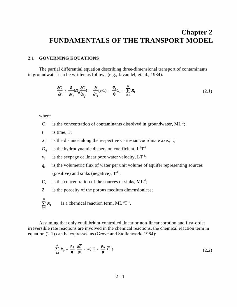
The partial differential equation describing three-dimensional transport of contaminantsin groundwater can be written as follows (e.g., Javandel, et. al., 1984):
(2.1)
where
C is the concentration of contaminants dissolved in groundwater, ML ;-3
t is time, T;
X is the distance along the respective Cartesian coordinate axis, L;i
D is the hydrodynamic dispersion coefficient, L Tij2 -1
v is the seepage or linear pore water velocity, LT ;j-1
q is the volumetric flux of water per unit volume of aquifer representing sourcess
(positive) and sinks (negative), T ;-1
C is the concentration of the sources or sinks, ML ;s-3
2 is the porosity of the porous medium dimensionless;
is a chemical reaction term, ML T .-3 -1
Assuming that only equilibrium-controlled linear or non-linear sorption and first-orderirreversible rate reactions are involved in the chemical reactions, the chemical reaction term inequation (2.1) can be expressed as (Grove and Stollenwerk, 1984):
(2.2)
2 - 2
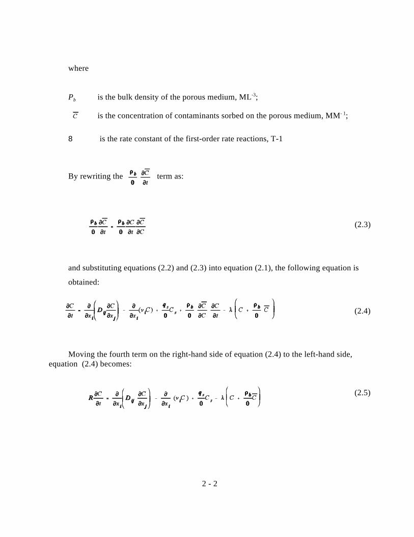
where
P is the bulk density of the porous medium, ML ;b-3
is the concentration of contaminants sorbed on the porous medium, MM ; - 1
8 is the rate constant of the first-order rate reactions, T-1
By rewriting the term as:
(2.3)
and substituting equations (2.2) and (2.3) into equation (2.1), the following equation is
obtained:
(2.4)
Moving the fourth term on the right-hand side of equation (2.4) to the left-hand side,equation (2.4) becomes:
(2.5)

2 - 3
where R is called the retardation factor, defined as
(2.6)
Equation (2.5) is the governing equation underlying in the transport model. The transportequation is linked to the flow equation through the relationship:
(2.7)
where
K is a principal component of the hydraulic conductivity tensor, LT ii-1
h is hydraulic head, L.
The hydraulic head is obtained from the solution of the three-dimensional groundwaterflow equation:
(2.8)
where
S, is the specific storage of the porous materials, L .-1
Note that the hydraulic conductivity tensor (K) actually has nine components. However,it is generally assumed that the principal components of the hydraulic conductivity tensor (K ,ii
or K , K , K .) are aligned with the x, y and z coordinate axes so that non-principalxx yy zz
components become zero. This assumption is incorporated in most commonly used flowmodels, including MODFLOW.
2 - 4
2.2 ADVECTION
The second term on the right-hand side of equation (2.5), , is referred to as the
advection term. The advection term describes the transport of miscible contaminants at thesame velocity as the groundwater. For many practical problems concerning contaminanttransport in groundwater, the advection term dominates. To measure the degree of advectiondomination, a dimensionless Peclet number is usually used. The Peclet number is defined as:
(2.9)
where
is the magnitude of the seepage velocity vector, LT ;-1
L is a characteristic length, commonly taken as the grid cell width, L;
D is the dispersion coefficient, L T .2 -l
In advection-dominated problems, also referred to as sharp front problems, the Pecletnumber has a large value. For pure advection problems, the Peclet number becomes infinite.
For advection-dominated problems, the solution of the transport equation by manystandard numerical procedures is plagued to some degree by two types of numerical problemsas illustrated in Fig. 2.1. The first type is numerical dispersion, which has an effect similar tothat of physical dispersion, but is caused by truncation error. When physical dispersion is smallor negligible, numerical dispersion becomes a serious problem, leading to the smearing ofconcentration fronts which should have a sharp appearance (Fig. 2. la). The second type ofnumerical problem is artificial oscillation, sometimes also referred to as overshoot andundershoot, as illustrated in Fig. 2.lb. Artificial oscillation is typical of many higher-orderschemes designed to eliminate numerical dispersion, and tends to become more severe as theconcentration front becomes sharper.
The mixed Eulerian-Lagrangian method implemented in the MT3D transport model isvirtually free of numerical dispersion and artificial oscillation and is capable of handling theentire range of Peclet numbers from 0 to as discussed in the next chapter.

2 - 5
2.3 DISPERSION
2.3.1 Dispersion Mechanism
Dispersion in porous media refers to the spreading of contaminants over a greaterregionthan would be predicted solely from the groundwater velocity vectors. As described byAnderson (1984), dispersion is caused by mechanical dispersion, a result of deviations of actualvelocity on a microscale from the average groundwater velocity, and molecular diffusion, aresult of concentration variations. The molecular diffusion effect is generally secondary andnegligible compared to the mechanical dispersion effect, and only becomes important whengroundwater velocity is very low. The sum of the mechanical dispersion and the moleculardiffusion is termed hydrodynamic dispersion.
Fig. 2.1. Illustration of common numerical errors in contaminant transport modeling.
Although the dispersion mechanism is generally understood, the representation ofdispersion phenomena in a transport model is the subject of intense continuing research. The
dispersion term in equation (2.5), represents a pragmatic approach through which
realistic transport calculations can be made without fully describing the heterogeneous velocityfield, which, of course, is impossible to do in practice. While many different approaches andtheories have been developed to represent the dispersion process, equation (2.5) is still the basisfor most practical simulations.
2.3.2 Dispersion Coefficient
The hydrodynamic dispersion tensor for isotropic porous media is defined, according toBear (1979), in the following component forms:
(2.9a)
2 - 6
(2.9b)
(2.9c)
(2.9d)
(2.9e)
(2.9f)
where
" is the longitudinal dispersivity, L;L
" is the transverse dispersivity, L;T
D* is the effective molecular diffusion coefficient, L T ;2 -1
v , v , v , are components of the velocity vector along the x, y, and z axes, LT ; x y z- 1
is the magnitude of the velocity vector, LT .- 1
Strictly speaking, the dispersion tensor defined by two independent dispersivities forisotropic media as in equations (2.9a) to (2.9f) is not valid for anisotropic porous media, whichrequire five independent dispersivities (Bear, 1979). Unfortunately, it is generally not feasibleto obtain all five dispersivities in the field. As a result, the usual practice in transport modelingis to assume that the isotropic dispersion coefficient is also applicable to anisotropic porousmedia.

2 - 7
In addition to the isotropic dispersion described above, the MT3D transport modelsupports an alternative form which allows the use of two transverse dispersivities, a horizontaltransverse dispersivity (" ) and a vertical transverse dispersivity (" ), as proposed by BurnettTH TV
and Frind (1987):
(2.10a)
(2.10b)
(2.10c)
(2.10d)
(2.10e)
(2. 10f)
Equations (2.10a) to (2.10f) become equivalent to equations (2.9a) to (2.9f) when the twotransverse dispersivities are set equal.
2.4 SINKS AND SOURCES
The third term in the governing equation, , is the sink/source term, which
represents solute mass dissolved in water entering the simulated domain through sources, orsolute mass dissolved in water leaving the simulated domain through sinks.
Sinks or sources may be classified as areally distributed or point sinks or sources. Theareally distributed sinks or sources include recharge and evapotranspiration. The point sinks or
2 - 8
sources include wells, drains, and rivers. Constant-head and general head dependentboundaries in the flow model are also treated as point sinks or sources because they function inexactly the same way as wells, drains, or rivers in the transport model.
For sources, it is necessary to specify the concentration of source water. For sinks, theconcentration of sink water is generally equal to the concentration of groundwater in theaquffer and should not be specified. However, there is one exception where the concentrationof sinks may differ from that of groundwater. The exception is evapotranspiration, which maybe assumed to take only pure water away from the aquifer so that the concentration of theevapotranspiration flux is zero.
2.5 CHEMICAL REACTIONS
The chemical reactions included in the MT3D transport model are equilibrium-controlledlinear or non-linear sorption and first-order irreversible rate reactions -- most commonly,radioactive decay or biodegradation. More sophisticated chemical reactions can be added tothe model when necessary without modifying the existing program.
2.5.1 Linear or Non-linear Sorption
Sorption refers to the mass transfer process between the contaminants dissolved ingroundwater (solution phase) and the contaminants sorbed on the porous medium (solid phase). It is generally assumed that equilibrium conditions exist between the solution-phase and solid--phase concentrations and that the sorption reaction is fast enough relative to groundwatervelocity so that it can be treated as instantaneous. The functional relationship between thedissolved and sorbed concentrations is called the sorption isotherm. Sorption isotherms aregenerally incorporated into the transport model through the use of the retardation factor (e.g.,Goode and Konikow, 1989). Three types of sorption isotherms are considered in the MT3Dtransport model: linear, Freundlich and Langmuir.
The linear sorption isotherm assumes that the sorbed concentration ( ) is directly
proportional to the dissolved concentration (C):
(2.11)
where ,K is called the distribution coefficient, L M . The retardation factor is defined asd3 -1
(2.12)

2 - 9
The Freundlich isotherm is a non-linear isotherm, expressed in the following form:
(2.13)
where
K is the Freundlich constant, (L M ) ;f3 -1 a
a is the Freundlich exponent, dimensionless.
Both K and a are empirical coefficients. When a is equal to 1, the Freundlich isotherm isf
equivalent to the linear isotherm. The retardation factor for the Freundlich isotherm is definedaccordingly as:
(2.14)
Another non-linear sorption isotherm is the Langmuir isotherm, described by
(2.15)
where
K is the Langmuir constant, L Ml3 -1
is the total concentration of sorption sites available, MM .-1
The retardation factor defined for the Langrnuir isotherm is then
(2.16)

2 - 10
2.5.2 Radioactive Decay or Biodegradation
The first-order irreversible rate reaction term included in the governing
equation, , represents the mass loss of both the dissolved phase (C) and the
sorbed phase with the same rate constant rate (8). The rate constant is usually given in
terms of the half-life:
(2.17)
where t is the half-life of radioactive or biodegradable materials, or the time required1/2for the concentration to decrease to one-half of the original value.
For certain types of biodegradation, the rate constant for the dissolved and sorbed phasesmay be different. Thus, in the MT3D model, two general rate constants are used: one for thedissolved phase (8 ) and the other for the sorbed phase (8 ) as shown below:1 2
(2.18)
The two constants should be set equal if the rate reaction simulated is radioactive decay,since radioactive decay generally occurs at the same rate in both phases. If the simulatedreaction is biodegradation, the two rate constants can be entered as different values.
It should be noted that the biodegradation process in the subsurface is complex and oftendoes not follow the first-order rate reaction equation (e.g., Suflita, et. al., 1987). Alternativeformulation for simulating biodegradation could be developed and added to the MT3D modelas a new option in the future.
2.6 INITIAL CONDITIONS
The governing equation of the transport model describes the transient changes of soluteconcentration in groundwater. Therefore, initial conditions are necessary to obtain a solution ofthe governing equation. The initial condition in general form is written as
(2.19)

2 - 11
where
CE (x, y, z) is a known concentration distribution and œ denotes the simulated domain.
2.7 BOUNDARY CONDITIONS
The solution of the governing equation also requires specification of boundary conditions. Three general types of boundary condition are considered in the MT3D transport model: (a)concentration known around a boundary (Dirichlet Condition), (b) concentration gradientknown across a boundary (Neumann Condition); and (c) a combination of (a) and (b).
For the first type of boundary condition, the concentration is specified along the boundaryand remains unchanged throughout the simulation, or,
(2.20)
where ' , denotes the specified-concentration boundary, and CE(x,y,z) is the specified1concentration along ' .1
In a flow model, a Dirichlet boundary is a specified-head boundary which acts as a sourceor sink of water entering or leaving the simulated domain. Similarly, a specified-concentrationboundary in a transport model acts as a source providing solute mass to the unulated domain, oras a sink taking solute mass out of the simulated domain. A specified-head boundary in theflow model may or may not be a specified-concentration boundary in the transport model.
For the second type of boundary condition, the concentration gradient is specified acrossthe boundary, or,
(2.21)
where q(x, y, z, t) is a known function representing the dispersive flux normal to theboundary ' . A special case is along impermeable boundaries where q(x, y, z, t) = 0.2
For the third type of boundary condition, both the concentration and concentration gradientare specified, or,
(2.22)
2 - 12
where g(x, y, z, t) is a known function representing the total flux (dispersive and advective)normal to the boundary ' . For impermeable boundaries, both dispersive and advective fluxes3are equal to zero so that g(x, y, z, t) = 0. On inflow or outflow boundaries, it is customary toassume that the advective flux dominates over the dispersive flux so that the above equationcan be simplified to
(2.23)
Equation (2.23) can be accommodated readily in the sink/source term of the governingequation.

3 - 1
Chapter 3EULERIAN-LAGRANGIAN SOLUTION
3.1 EULERIAN-LAGRANGIAN EQUATIONS
According to the chain rule, the advection term in governing equation (2.5) can beexpanded to
(3.1)
Substituting equation (3. 1) into equation (2.5) and dividing both sides by the retardationfactor, the governing equation becomes
(3.2)
where, , represents the "retarded" velocity of a contaminant particle.
Equation (3.2) is an Eulerian expression in which the partial derivative, , indicates
the rate of change in solute concentration (C) at a fixed point in space. Equation (3.2) can
also be expressed in the Lagrangian form as
(3.3)
where the substantial derivative, , indicates the rate of change in solute
concentration (C) along the pathline of a contaminant particle (or a characteristic curve of thevelocity field).
By introducing the finite-difference algorithm, the substantial derivative in equation(3.3) can be approximated as
(3.4)
3 - 2
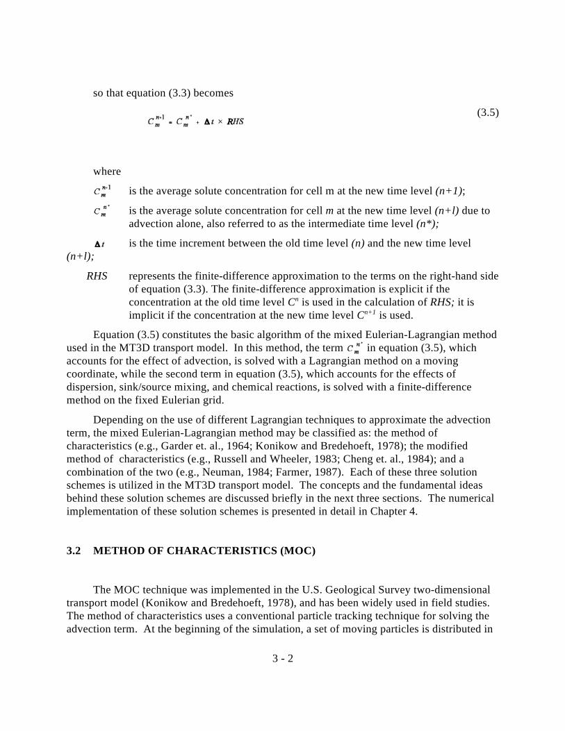
so that equation (3.3) becomes
(3.5)
where
is the average solute concentration for cell m at the new time level (n+1);
is the average solute concentration for cell m at the new time level (n+l) due toadvection alone, also referred to as the intermediate time level (n*);
is the time increment between the old time level (n) and the new time level(n+l);
RHS represents the finite-difference approximation to the terms on the right-hand sideof equation (3.3). The finite-difference approximation is explicit if theconcentration at the old time level C is used in the calculation of RHS; it isn
implicit if the concentration at the new time level C is used.n+1
Equation (3.5) constitutes the basic algorithm of the mixed Eulerian-Lagrangian methodused in the MT3D transport model. In this method, the term in equation (3.5), whichaccounts for the effect of advection, is solved with a Lagrangian method on a movingcoordinate, while the second term in equation (3.5), which accounts for the effects ofdispersion, sink/source mixing, and chemical reactions, is solved with a finite-differencemethod on the fixed Eulerian grid.
Depending on the use of different Lagrangian techniques to approximate the advectionterm, the mixed Eulerian-Lagrangian method may be classified as: the method ofcharacteristics (e.g., Garder et. al., 1964; Konikow and Bredehoeft, 1978); the modifiedmethod of characteristics (e.g., Russell and Wheeler, 1983; Cheng et. al., 1984); and acombination of the two (e.g., Neuman, 1984; Farmer, 1987). Each of these three solutionschemes is utilized in the MT3D transport model. The concepts and the fundamental ideasbehind these solution schemes are discussed briefly in the next three sections. The numericalimplementation of these solution schemes is presented in detail in Chapter 4.
3.2 METHOD OF CHARACTERISTICS (MOC)
The MOC technique was implemented in the U.S. Geological Survey two-dimensional transport model (Konikow and Bredehoeft, 1978), and has been widely used in field studies. The method of characteristics uses a conventional particle tracking technique for solving theadvection term. At the beginning of the simulation, a set of moving particles is distributed in
3 - 3
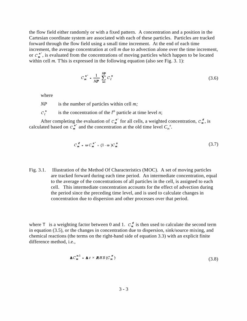
the flow field either randomly or with a fixed pattern. A concentration and a position in theCartesian coordinate system are associated with each of these particles. Particles are trackedforward through the flow field using a small time increment. At the end of each timeincrement, the average concentration at cell m due to advection alone over the time increment,or , is evaluated from the concentrations of moving particles which happen to be locatedwithin cell m. T'his is expressed in the following equation (also see Fig. 3. 1):
(3.6)
where
NP is the number of particles within cell m;
is the concentration of the l particle at time level n;th
After completing the evaluation of for all cells, a weighted concentration, , iscalculated based on and the concentration at the old time level C .m
n
(3.7)
Fig. 3.1. Illustration of the Method Of Characteristics (MOC). A set of moving particlesare tracked forward during each time period. An intermediate concentration, equalto the average of the concentrations of all particles in the cell, is assigned to eachcell. This intermediate concentration accounts for the effect of advection duringthe period since the preceding time level, and is used to calculate changes inconcentration due to dispersion and other processes over that period.
where T is a weighting factor between 0 and 1. is then used to calculate the second termin equation (3.5), or the changes in concentration due to dispersion, sink/source mixing, andchemical reactions (the terms on the right-hand side of equation 3.3) with an explicit finitedifference method, i.e.,
(3.8)
3 - 4
The use of the weighted concentration in equation (3.8) represents an averagedapproach because the precesses of dispersion, sink/source mixing, and/or chemical reactionsoccur throughout the time increment.
The concentration for cell m at the new time level (n+1) is then the sum of the and terms. The concentrations of all moving particles are also updated to reflect the change
due to dispersion, sink/source mixing, and chemical reactions. This completes the calculationof one transport step for the method of characteristics. The procedure is repeated until the endof a desired time period is reached.
One of the most desirable features of the MOC technique is that it is virtually free ofnumerical dispersion, which creates serious difficulty in many standard numerical schemes. The major drawback of the MOC technique is that it can be slow and requires a large amountof computer memory when it is necessary to track a large number of moving particles,especially in three dimensions. The MOC technique can also lead to large mass balancediscrepancies under certain situations because the MOC technique, like other mixed Eulerian-Lagrangian solution techniques, is not entirely based on the principle of mass conservation. In the MT3D transport model, the computer memory requirement for the MOC technique isdramatically reduced through the use of a dynamic approach for particle distribution. Themass balance discrepancy problem is also overcome to a large extent through the use ofconsistent velocity interpolation schemes and higher-order particle tracking algorithms. Further discussion of these topics is given in the next chapter.
3.3 MODIFIED METHOD OF CHARACTERISTICS (MMOC)
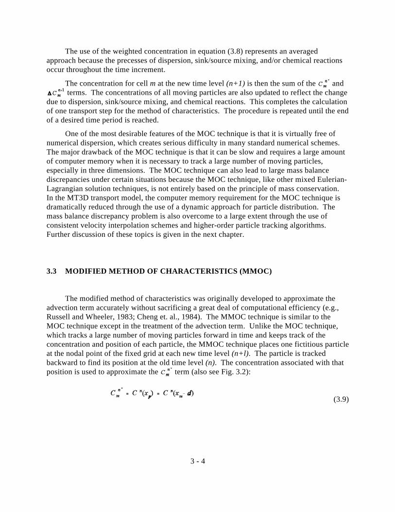
The modified method of characteristics was originally developed to approximate theadvection term accurately without sacrificing a great deal of computational efficiency (e.g.,Russell and Wheeler, 1983; Cheng et. al., 1984). The MMOC technique is similar to theMOC technique except in the treatment of the advection term. Unlike the MOC technique,which tracks a large number of moving particles forward in time and keeps track of theconcentration and position of each particle, the MMOC technique places one fictitious particleat the nodal point of the fixed grid at each new time level (n+l). The particle is trackedbackward to find its position at the old time level (n). The concentration associated with thatposition is used to approximate the term (also see Fig. 3.2):
(3.9)
3 - 5
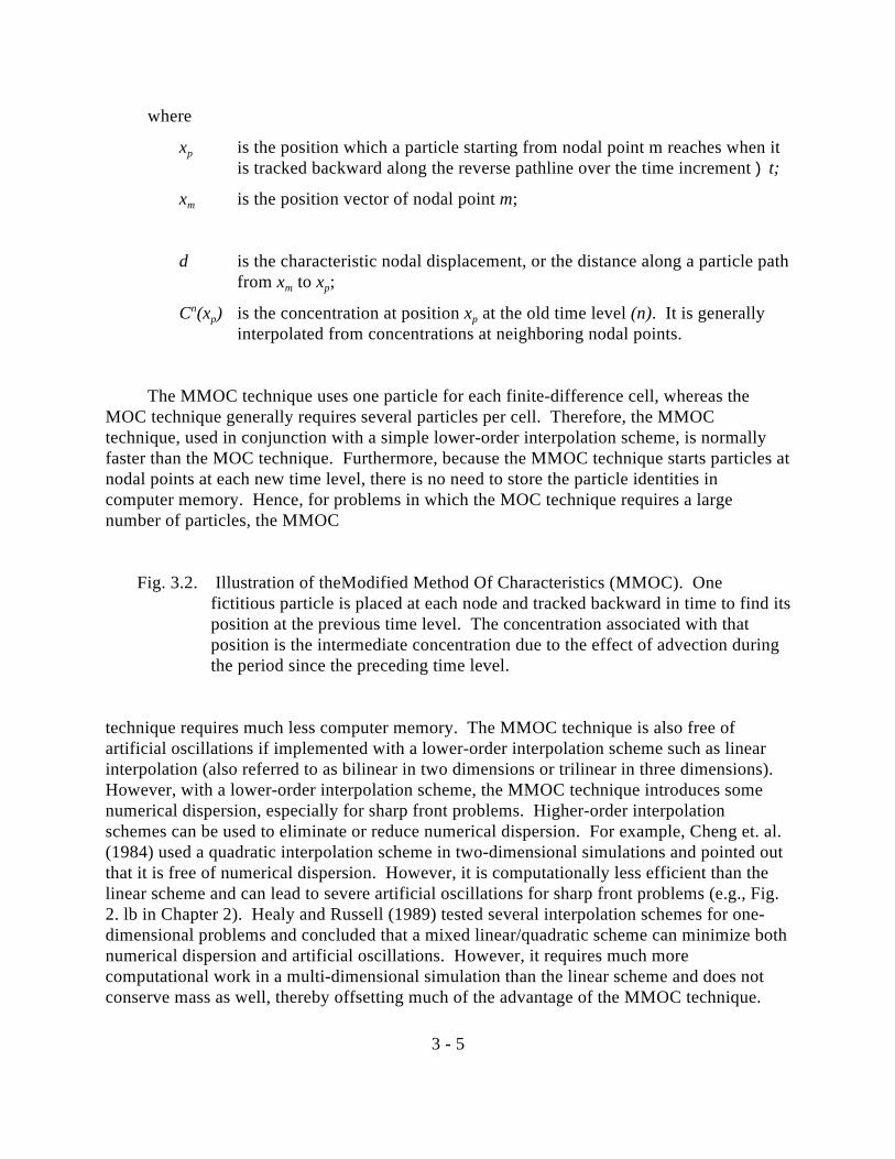
where
x is the position which a particle starting from nodal point m reaches when itp
is tracked backward along the reverse pathline over the time increment )t;
x is the position vector of nodal point m;m
d is the characteristic nodal displacement, or the distance along a particle pathfrom x to x ;m p
C (x ) is the concentration at position x at the old time level (n). It is generallynp p
interpolated from concentrations at neighboring nodal points.
The MMOC technique uses one particle for each finite-difference cell, whereas theMOC technique generally requires several particles per cell. Therefore, the MMOCtechnique, used in conjunction with a simple lower-order interpolation scheme, is normallyfaster than the MOC technique. Furthermore, because the MMOC technique starts particles atnodal points at each new time level, there is no need to store the particle identities incomputer memory. Hence, for problems in which the MOC technique requires a largenumber of particles, the MMOC
Fig. 3.2. Illustration of theModified Method Of Characteristics (MMOC). Onefictitious particle is placed at each node and tracked backward in time to find itsposition at the previous time level. The concentration associated with thatposition is the intermediate concentration due to the effect of advection duringthe period since the preceding time level.
technique requires much less computer memory. The MMOC technique is also free ofartificial oscillations if implemented with a lower-order interpolation scheme such as linearinterpolation (also referred to as bilinear in two dimensions or trilinear in three dimensions). However, with a lower-order interpolation scheme, the MMOC technique introduces somenumerical dispersion, especially for sharp front problems. Higher-order interpolationschemes can be used to eliminate or reduce numerical dispersion. For example, Cheng et. al.(1984) used a quadratic interpolation scheme in two-dimensional simulations and pointed outthat it is free of numerical dispersion. However, it is computationally less efficient than thelinear scheme and can lead to severe artificial oscillations for sharp front problems (e.g., Fig.2. lb in Chapter 2). Healy and Russell (1989) tested several interpolation schemes for one-dimensional problems and concluded that a mixed linear/quadratic scheme can minimize bothnumerical dispersion and artificial oscillations. However, it requires much morecomputational work in a multi-dimensional simulation than the linear scheme and does notconserve mass as well, thereby offsetting much of the advantage of the MMOC technique.
3 - 6
For these reasons, the MMOC technique in the MT3D transport model is implemented onlywith a lower-order interpolation scheme and is intended for use in situations where sharpfronts are not present, so that any numerical dispersion error resulting from the solutionscheme is insignificant.
3.4 HYBRID METHOD OF CHARACTERISTICS (HMOC)
As shown in the preceding discussions, either the MOC or the MMOC scheme may beutilized to solve the mixed Eulerian-Lagrangian equation. The selection of the method isbased on such considerations as field conditions (whether the concentration field has sharp orsmooth fronts) and computer resources available (generally the MOC solution requires morememory space and longer execution time). A third option is to use a hybrid of the twomethods; this option is referred to here as the hybrid method of characteristics (HMOC).
The HMOC technique attempts to combine the strengths of the MOC and the MMOCtechniques by using an automatic adaptive scheme conceptually similar to the one proposedby Neuman (1984). The fundamental idea behind this scheme is automatic adaptation of thesolution process to the nature of the concentration field. When sharp concentration fronts arepresent, the advection term is solved by the MOC technique through the use of movingparticles dynamically distributed around each front. Away from such fronts, the advectionterm is solved by the MMOC technique with fictitious particles placed at the nodal pointsdirectly tracked backward in time. When a front dissipates due to dispersion and chemicalreactions, the forward tracidng stops automatically and the corresponding particles areremoved. By selecting an appropriate criterion for controlling the switch between the MOCand MMOC schemes, the adaptive procedure can provide accurate solutions to transportproblems over the entire range of Peclet numbers fiom 0 to4 with virtually no numericaldispersion, while at the same time using far fewer particles than would be required by theMOC scheme alone.
Under certain circumstances, the choice for the adaptive criterion used in the HMOCscheme may not be obvious and the adaptive procedure may not lead to an optimal solution. In these cases, manual selection of either the MOC or the MMOC scheme may be moreefficient. Therefore, all of the these three solution schemes are included in the current versionof the MT3D transport model.
4 - 1
Chapter 4NUMERICAL IMPLEMENTATION
4.1 SPATIAL DISCRETIZATION
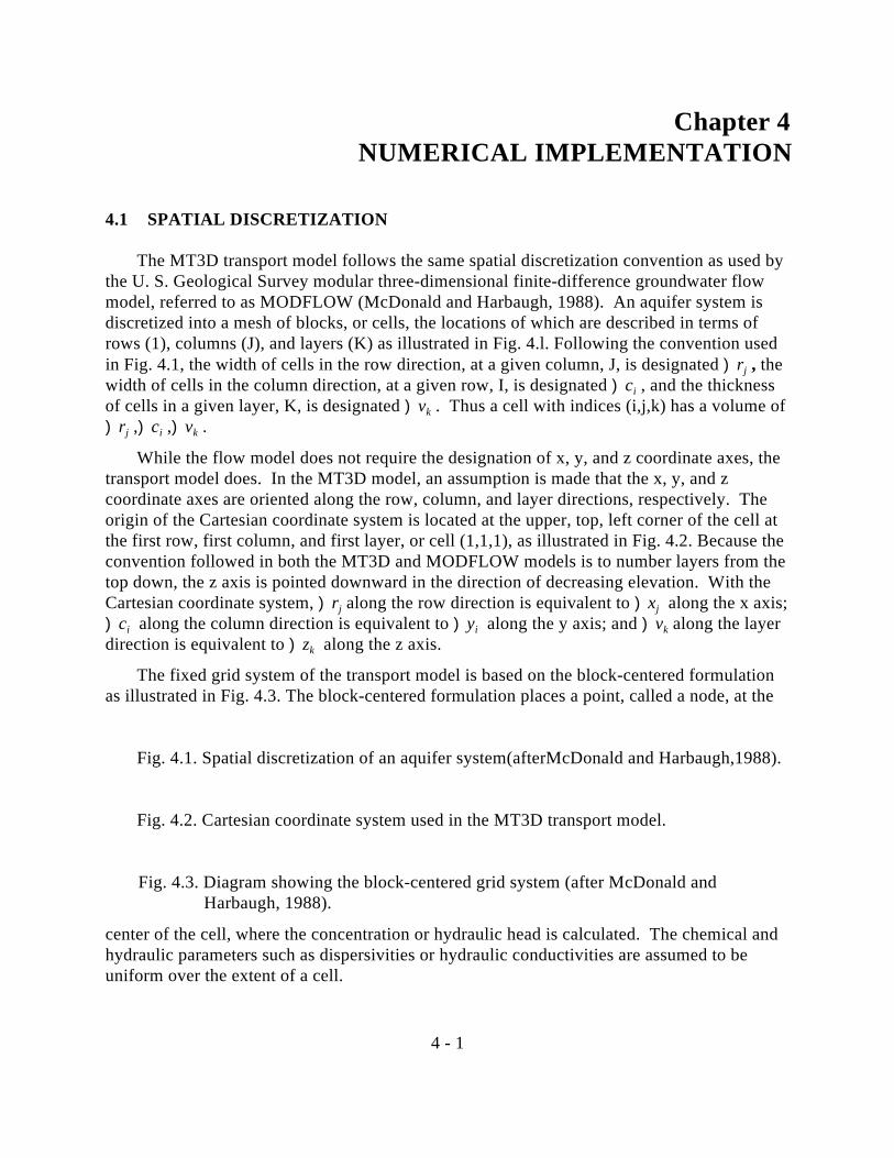
The MT3D transport model follows the same spatial discretization convention as used bythe U. S. Geological Survey modular three-dimensional finite-difference groundwater flowmodel, referred to as MODFLOW (McDonald and Harbaugh, 1988). An aquifer system isdiscretized into a mesh of blocks, or cells, the locations of which are described in terms ofrows (1), columns (J), and layers (K) as illustrated in Fig. 4.l. Following the convention usedin Fig. 4.1, the width of cells in the row direction, at a given column, J, is designated )r , thej
width of cells in the column direction, at a given row, I, is designated )c , and the thicknessi
of cells in a given layer, K, is designated )v . Thus a cell with indices (i,j,k) has a volume ofk
)r ,)c ,)v .j i k
While the flow model does not require the designation of x, y, and z coordinate axes, thetransport model does. In the MT3D model, an assumption is made that the x, y, and zcoordinate axes are oriented along the row, column, and layer directions, respectively. Theorigin of the Cartesian coordinate system is located at the upper, top, left corner of the cell atthe first row, first column, and first layer, or cell (1,1,1), as illustrated in Fig. 4.2. Because theconvention followed in both the MT3D and MODFLOW models is to number layers from thetop down, the z axis is pointed downward in the direction of decreasing elevation. With theCartesian coordinate system, )r along the row direction is equivalent to )x along the x axis;j j
)c along the column direction is equivalent to )y along the y axis; and )v along the layeri i k
direction is equivalent to )z along the z axis.k
The fixed grid system of the transport model is based on the block-centered formulationas illustrated in Fig. 4.3. The block-centered formulation places a point, called a node, at the
Fig. 4.1. Spatial discretization of an aquifer system(afterMcDonald and Harbaugh,1988).
Fig. 4.2. Cartesian coordinate system used in the MT3D transport model.
Fig. 4.3. Diagram showing the block-centered grid system (after McDonald andHarbaugh, 1988).
center of the cell, where the concentration or hydraulic head is calculated. The chemical andhydraulic parameters such as dispersivities or hydraulic conductivities are assumed to beuniform over the extent of a cell.
4 - 2
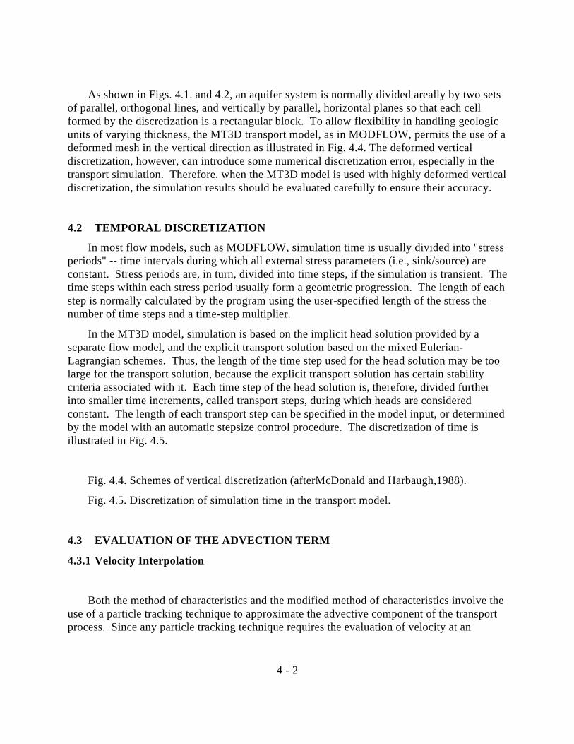
As shown in Figs. 4.1. and 4.2, an aquifer system is normally divided areally by two setsof parallel, orthogonal lines, and vertically by parallel, horizontal planes so that each cellformed by the discretization is a rectangular block. To allow flexibility in handling geologicunits of varying thickness, the MT3D transport model, as in MODFLOW, permits the use of adeformed mesh in the vertical direction as illustrated in Fig. 4.4. The deformed verticaldiscretization, however, can introduce some numerical discretization error, especially in thetransport simulation. Therefore, when the MT3D model is used with highly deformed verticaldiscretization, the simulation results should be evaluated carefully to ensure their accuracy.
4.2 TEMPORAL DISCRETIZATION
In most flow models, such as MODFLOW, simulation time is usually divided into "stressperiods" -- time intervals during which all external stress parameters (i.e., sink/source) areconstant. Stress periods are, in turn, divided into time steps, if the simulation is transient. Thetime steps within each stress period usually form a geometric progression. The length of eachstep is normally calculated by the program using the user-specified length of the stress thenumber of time steps and a time-step multiplier.
In the MT3D model, simulation is based on the implicit head solution provided by aseparate flow model, and the explicit transport solution based on the mixed Eulerian-Lagrangian schemes. Thus, the length of the time step used for the head solution may be toolarge for the transport solution, because the explicit transport solution has certain stabilitycriteria associated with it. Each time step of the head solution is, therefore, divided furtherinto smaller time increments, called transport steps, during which heads are consideredconstant. The length of each transport step can be specified in the model input, or determinedby the model with an automatic stepsize control procedure. The discretization of time isillustrated in Fig. 4.5.
Fig. 4.4. Schemes of vertical discretization (afterMcDonald and Harbaugh,1988).
Fig. 4.5. Discretization of simulation time in the transport model.
4.3 EVALUATION OF THE ADVECTION TERM
4.3.1 Velocity Interpolation
Both the method of characteristics and the modified method of characteristics involve theuse of a particle tracking technique to approximate the advective component of the transportprocess. Since any particle tracking technique requires the evaluation of velocity at an

4 - 3
arbitrary point from hydraulic heads calculated at nodal points, it is necessary to use avelocity interpolation scheme in the particle tracking calculations.
The velocity interpolation scheme used in this transport model is simple piecewise linearinterpolation (e.g., Pollock, 1988; Zheng, 1988). This scheme assumes that a velocitycomponent varies linearly within a finite-difference cell with respect to the direction of thatcomponent. Thus, the x-component of the Darcy velocity at an arbitrary point within a cell(i,j,k) can be expressed in terms of the fluxes on cell interfaces in the same direction (Fig.4.6):
(4.1)
where
, is the flux, or the specific discharge, through the
interface between cells (i,j-l,k) and (i,j,k), and K is the harmonic mean ofi,,j-1/2,k
hydraulic conductivity between the two cells. The flux at the cell interface iscalculated in the flow model and directly used in the transport model;
is the flux through the interface between cells
(i,j,k) and (i,j+l,k);
is the linear interpolation factor for the x component;
x , y , z , are the Cartesian coordinates of the particle location;p p p
is the x coordinates of the left and right interfaces of the cell (i,j,k);
x is the x coordinates of the node (i,j,k); andj
)x is the cell width along the x-axis at cell (i,j,)j
Fig. 4.6. The velocity interpolation scheme used in particle tracking.

4 - 4
The x-component of the linear or pore water velocity, v , is then obtained from:x
(4.2)
where 2 is the porosity value at cell (i,j,k).i, j,k
Similarly, the y- and z- components of the velocity are calculated as:
(4.3)
(4.4)
where is the linear interpolation factor for the y-component; and
(4.5)
(4.6)
where is the linear interpolation factor for the z- component.
The velocity field generated with this scheme is consistent with the block-centered finite-difference formulation of the three-dimensional flow equation, and thus conserves masslocally within each finite-difference block. It also preserves the velocity discontinuitiescaused by changes in hydraulic conductivities present in heterogeneous media.
It is noted that this velocity scheme differs from the multi-linear scheme used in earliermethod-of-characteristics models (e.g., Garder et. al., 1964; Konikow and Bredehoeft, 1978). The multi-linear scheme in a three-dimensional flow field assumes that velocity components
4 - 5
vary linearly in all three directions, and thus generates a continuous velocity field in everydirection. Goode (1990) notes that the multi-linear scheme may result in more satisfactoryresults in homogeneous media. However, the multi-linear scheme is not consistent with thecell-by-cell mass balance described by the block-centered finite-difference formulation anddoes not preserve the velocity discontinuities present in heterogeneous media, unlike thepiecewise linear scheme. Because of this and because the piecewise linear scheme iscomputationally much more efficient, the piecewise linear scheme has been utilized in theMT3D model.
4.3.2 Particle Tracking
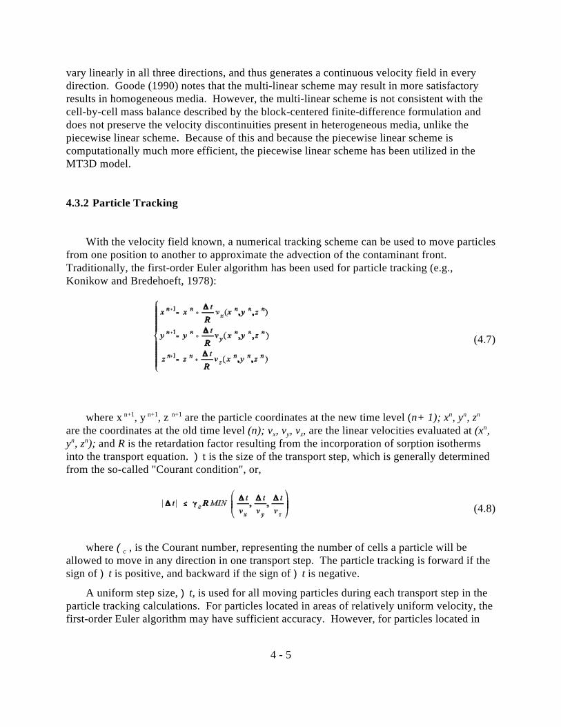
With the velocity field known, a numerical tracking scheme can be used to move particlesfrom one position to another to approximate the advection of the contaminant front. Traditionally, the first-order Euler algorithm has been used for particle tracking (e.g.,Konikow and Bredehoeft, 1978):
(4.7)
where x , y , z are the particle coordinates at the new time level (n+ 1); x , y , z n+1 n+1 n+1 n n n
are the coordinates at the old time level (n); v , v , v , are the linear velocities evaluated at (x ,x y zn
y , z ); and R is the retardation factor resulting from the incorporation of sorption isothermsn n
into the transport equation. )t is the size of the transport step, which is generally determinedfrom the so-called "Courant condition", or,
(4.8)
where ( , is the Courant number, representing the number of cells a particle will bec
allowed to move in any direction in one transport step. The particle tracking is forward if thesign of )t is positive, and backward if the sign of )t is negative.
A uniform step size, )t, is used for all moving particles during each transport step in theparticle tracking calculations. For particles located in areas of relatively uniform velocity, thefirst-order Euler algorithm may have sufficient accuracy. However, for particles located in

4 - 6
areas of strongly converging or diverging flows, for example, near sources or sinks, the first--order algorithm may not be sufficiently accurate, unless )t is very small. In these cases ahigher-order algorithm such as the fourth-order Runge-Kutta method may be used (e.g.,Zheng, 1988). The basic idea of the fourth-order Runge-Kutta method is to evaluate thevelocity four times for each tracking step: once at the initial point, twice at two trialmidpoints, and once at a trial end point (Fig. 4.7). A weighted velocity based on valuesevaluated at these four points is used to move the particle to the new position ( x , y , zn+1 n+1
). This process may be expressed as follows:n+1
(4.9)
where

4 - 7
Fig. 4.7. The fourth-order Runge-Kutta method. In each step, the velocity is evaluated fourtimes: once at the initial point, twice at trial midpoints, and once at a trial endpoint. From these velocities a weighted velocity is calculated which is used to compute thefinal position of the particle (shown as a filled dot). (Modified from Press el. al.,1986).
The fourth-order Runge-Kutta algorithm is more accurate and permits the use of largertracking steps. However, the computational effort required by the fourth-order Runge-Kuttaalgorithm is considerably more than that required by the Euler algorithm, making the formerless efficient than the latter for three-dimensional simulations when a very large number ofparticles are used. For these reasons, the MT3D model provides three options: a first-orderEuler algorithm, a fourth-order Runge-Kutta algorithm, and a combination of these two. These options, when used properly, allow sufficient accuracy throughout the finite-differencegrid without using exceedingly small stepsizes.
4.3.3 The MOC Procedure
The first step in the method of characteristics is to generate representative particles in the finite-difference grid. Instead of placing a uniform number of particles in every cell of thegrid, a dynamic approach is used in the MT3D transport model to control the distribution ofmoving particles. The number of particles placed at each cell is normally set either at a highlevel or at a low level, according to the so-called "relative cell concentration gradient", or,DCCELL, defined as:
(4.10)
where
, is the maximum concentration in the immediatevicinity of the cell (i,j,k);
, is the minimum concentration in the immediatevicinity of the cell (ijk);
CMAX is the maximum concentration in the entire grid; and
CMIIV is the minimum concentration in the entire grid.

4 - 8
With the dynamic approach, the user defines the criterion, DCEPS, which is a smallinteger number near zero; the higher number of particles, NPH, is placed in cells where therelative concentration gradient is greater than DCEPS, and the lower number of particles,NPL, in cells where the relative concentration gradient is less than DCEPS, i.e.,
(4.11)
where NPi,j,k is number of particles placed in cell (i,j,k).
Initially, if the concentration gradient at a cell is zero or small, (i.e., the concentrationfield is relatively constant near that cell), the number of particles placed in that cell is NPL,which may be zero or some small integer number, this is done because the concentrationchange due to advection between that cell and the neighboring cells will be insignificant. Ifthe concentration gradient at a cell is large, which indicates that the concentration field nearthat cell is rapidly changing, then the number of particles placed in that cell is NPH.
As particles leave source cells or accumulate at sink cells, it becomes necessary to insertnew particles at sources, or remove particles at sinks. At non-source or non-sink cells, it alsobecomes necessary to insert or remove particles as the cell concentration gradient changeswith time. This is done in the dynamic insertion-deletion procedure by specifying theminimum and maximum numbers of particles allowed per cell, called NPMIN and NPMAX,respectively. When the number of particles in any cell, (source or non-source), becomessmaller than the specified minimum, or NPMIN, new particles equal to NPL or NPH areinserted into that cell without affecting the existing particles. On the other hand, when thenumber of particle in any cell, (sink or non-sink), exceeds the specified maximum, or NP ,particles are removed from that cell until the maximum is met. To save computer storage,memory space occupied by the deleted particles is reused by newly inserted particles.
Fig. 4.8. Comparison of the uniform and dynamic appoaches in controlling thedistribution of moving particles.
Fig. 4.8 illustrates the dynamic particle distribution approach in contrast with the uniformapproach in simulating two-dimensional solute transport from a continuous point source in auniform flow field. Whereas the uniform approach inserts and maintains an approximatelyuniform particle distribution throughout the simulated domain, the dynamic approach adjuststhe distribution of moving particles dynamically, adapting to the changing nature of theconcentration field. In many practical problems involving contaminant transport modeling,the contaminant plumes may occupy only a small fraction of the finite-difference grid and theconcentrations may be changing rapidly only at sharp fronts. In these cases, the number of
4 - 9
total particles used is much smaller than that required in the uniform particle distributionapproach, thereby dramatically increasing the efficiency of the method-of-characteristicsmodel with little loss in accuracy.
Particles can be distributed either with a fixed pattern or randomly, as controlled by theuser-specified option (see Fig. 4.9). If the fixed pattern is chosen, the user determines not onlythe number of particles to be placed per cell, but also the pattern of the particle placement inplan view and the number of vertical planes on which particles are placed within each cellblock. If the random pattern is chosen, the user only needs to specify the number of particlesto be placed per cell. The program then calls a random number generator and distributes therequired number of particles randomly within each cell block. (The selection of these optionsis discussed in Chapter 6: Input Instructions). The fixed pattern may work better if the flowfield is relatively uniform. On the other hand, if the flow field is highly nonuniform withmany sinks or sources in largely heterogeneous media, the random pattern may capture theessence of the flow field better than the fixed pattern does.
Fig. 4.9. Initial placement of moving particles.
Each particle is associated with a set of attributes, that is, the x-, y-, and z-coordinates andthe concentration. The initial concentration of the particle is assigned as the concentration ofthe cell where the particle is initialized. At the beginning of each transport step, all particlesare moved over the time increment, At, using the particle tracking techniques describedpreviously. The x-, y-, and z-coordinates of the moving particles are then updated to reflecttheir new positions at the end of the transport step. The average concentration of a finite-difference cell at the end of the transport step due to advection alone, , is obtained byaccumulating the concentrations of all particles that are located at that cell, divided by thenumber of particles:
(4.12)
If the number of particles at the cell is zero, then the average concentration after particletracking is set equal to the cell concentration at the previous time level because theconcentration change at that cell over the time increment is either negligible or dominated byan external source:
(4.13)

4 - 10
It is necessary to locate the cell indices of any particle in the tracking and averagingcalculations as described above. If the finite-difference grid is regular, it is straightforward toconvert particle coordinates (x , y , z ,) to cell indices (JP, IP, KP) according to the followingp p p
formulas:
(4.14)
where INT(X) is a FORTRAN function, equal to the truncated value of x; and )x, )y, )zare the uniform grid spacings along the x-, y-, and z-axes. If the finite-difference grid isirregular, then, an efficient bisection routine is used to locate the cell indices from the x-, y-,and z-coordinates as illustrated in Fig. 4. 1 0.
Fig.4.10. To determine in which cell a particle P is located in an irregular mesh, asearching procedure is first started from a guessed position, either up ordown, in increments of one, two, then four, etc., until the desired value isbracketed. Second, a bisection routine is used to bisect the nodal points inthe immediate vicinity of the particle position, JLO and JHI. Finally, thecoordinate of the particle is compared with that of the interface between JLOand JHI to find out whether P is located in cell JW or cell JHI. In thisexample, if the guessed position were J = 7 instead of J = 2, the cell index ofP would have been located in far fewer steps. In the particle trackingcalculations, the next particle to be moved is usually adjacent to the particlethat has just been moved; thus the cell indices of the particle just moved areused as the guessed indices for the particle to be moved next.
After the term is evaluated at every cell, it is used to calculate the concentrationchange due to dispersion, sink/source mixing and/or chemical reactions ( ) using thefinite-difference method as discussed in Sections 4.4, 4.5 and 4.6. The concentration of allactive particles is then updated by adding the concentration change ( ) Calculated at thecell where each particle is located. Therefore, for moving particles located at cell (i,j,k):

4 - 11
(4.15)
where is the concentration of the l particle which is located at cell (i,j,k) at the newth
time level. If ) is positive, equation (4.15) is applied directly. However, if isnegative, the concentration of the moving particle may become negative if its concentration atthe old time level, , is zero or small. To prevent this from happening, a weightingprocedure, similar to the one used in Konikow and Bredehoeft (1978), is implemented whichplaces more weight on particles with higher concentrations than particles with lowerconcentrations in the same cell:
(4.16)
4.3.4 The MMOC Procedure
The first step in the MMOC procedure is to move a particle located at the nodal point ofthe cell backward in time using the particle tracking techniques. The purpose of thisbackward tracking is to find the position from which a particle would have originated at thebeginning of the time step so as to reach the nodal point at the end of the time step. Theconcentration associated withe that position, denoted as ( ) is the concentration of the celldue to advection alone over the time increment )t.
The position ( ) generally does not coincide with a nodal point. Thus, it is necessaryto interpolate the concentration at ( ) from concentrations at neighboring nodal points. The interpolation scheme used in the MT3D transport model is first-order polynomialinterpolation, also referred to as bilinear in two dimensions or trilinear in three dimensions. The general equation for first-order polynomial interpolation is as follows, assuming that islocated between nodes X and x , between , and y , and between z , and z (also see Fig. j-1 j i-1 k-1 k
4.1 1):
(4.17)

4 - 12
where T ,T , and T are interpolation factors as given below:x y z
(4.18)
If the x-, y-, or z-dimension is not simulated, the weighting factor in the respectivedirection is zero. If any cell is inactive, the cell is skipped in the calculation. The low-orderinterpolation represented by equation (4.17) is computationally very efficient and has smallmass balance error. It is also virtually free of artificial oscillation. However, this linearscheme does not eliminate numerical dispersion. As the concentration fronts become sharper,the amount of numerical dispersion increases. However, in the MT3D transport model, theMMOC scheme is only intended for problems with relatively smooth concentration fronts(sharp front problems are handled by the MOC technique). When the concentration field isrelatively smooth, the numerical dispersion resulting from the MMOC technique isinsignificant.
Fig. 4.11 Interpolation of the concentration at point P from the concentrations atneighboring nodes using the trilinear scheme in three dimensions.
Sinks or sources create special problems for the MMOC scheme, and thus have to betreated differently. First, examine a sink cell with inward hydraulic gradients on all of the cellinterfaces as illustrated in Fig. 4.12. If the sink is symmetric, the velocity at the nodal point iszero. Therefore, instead of placing one particle at the nodal point, the MT3D program placesmultiple particles within the cell. The number and distribution of these particles arecontrolled by the user-specified options in a manner similar to those described in the MOCprocedure. Each particle is tracked backward over )t, and its concentration is interpolated forneighboring nodes. The cell concentration is then averaged from the concentrations of allparticles, based on the reverse distance algorithm:
(4.19)

4 - 13
where d is the distance between the nodal point and the position where the l particle islth
initially placed. The reverse distance algorithm differs from the simple average algorithmused in the MOC scheme, in that the former gives more weight to particles that are locatedcloser to the node whereas the latter gives the same weight to all particles in the same cell.
Next, consider a source cell with outward hydraulic gradients on all cell interfaces. Backward tracking will cause particles placed in the source cell to converge toward the nodalpoint so that:
(4.20)
With the MMOC scheme, particles are restarted at each time step, and thus, there is noneed to store the particle locations and concentrations in computer memory. Thus, theMMOC solution normally requires far less computer memory, and is generally more efficientcomputationally than the MOC solution.
(a) At a sink cell with inward gradients on all interfaces
(b) Instead of placing one single particle at the node, multiple particles are placed andtracked backward. In this example, 8 particles distributed with a fixed pattern areused. However, both the number and the pattern can be changed in the user-specified options.
Fig. 4.12. Special treatment of sink cells in the MMOC scheme.
4.3.5 The HMOC Procedure
The forward-tracking MOC scheme is uniquely suitable for sharp front problems (pureadvection or largely advection-dominated problems) because it virtually eliminates numericaldispersion, a serious problem plaguing many standard numerical procedures. The MOCscheme implemented with dynamic particle distribution is also very efficient computationallyfor many practical problems where the contaminant plume occupies only a small fraction ofthe finite-difference grid, and the concentration field is changing rapidly only at sharp fronts. However, as the degree of advection domination over dispersion and chemical reactionsdecreases, the advantage of the MOC scheme is less obvious because as physical dispersionincreases, numerical dispersion becomes less of a problem. Furthermore, as large physicaldispersion causes the contaminant plume to spread through a large portion of the simulateddomain, the number of moving particles needed by the MOC scheme can become very large
4 - 14
for a three-dimensional simulation, pushing the memory requirement beyond the limits ofmany personal computers. The backward-tracking MMOC scheme tends to complement theMOC scheme for smooth front problems because the MMOC scheme requires far lesscomputer memory, is generally more efficient computationally and introduces very littlenumerical dispersion.
If the flow field and the dispersivity parameters are relatively constant, and the spatialdiscretization is fairly regular, it may be straightforward to select either the MOC or theMMOC scheme to be used in the simulation based on the mesh Peclet number:
(4.21)
where is the magnitude of the seepage velocity component; )x is the cell width along thei
i direction and D is the component of the dispersion coefficient with respect to that direction. ii
The MOC scheme is suitable for problems with large mesh Peclet numbers while the MMOCscheme can be used for problems with small mesh Peclet numbers. As a rule of thumb, theMOC scheme may be used effectively for problems with a mesh Peclet number greater than10 while the MMOC scheme may be used for problems with a mesh Peclet number smallerthan 0.1 without introducing any significant amount of numerical dispersion. It should bepointed out that this rule of thumb is based on a limited number of numerical experiments andmay not be true for all situations.
Under certain circumstances, the use of the MOC scheme alone may require too muchcomputer memory and execution time while the use of the MMOC scheme may lead tonoticeable numerical dispersion, so that neither provides a satisfactory solution. In thesecases, a hybrid scheme combining the MOC and MMOC schemes (or HMOC) may workbest. The fundamental idea behind the hybrid MOC/MMOC scheme is to combine thestrengths of the MOC and the MMOC techniques by using an automatic adaptive procedure,which causes MOC to be used in areas of steep concentration gradients and MMOC to beused in areas of low concentration gradients. The automatic selection is based on thesharpness of the concentration fronts, measured by the relative concentration gradientbetween the cell being considered and its neighboring cells as defined in equation 4.10. Theimplementation of the hybrid scheme is through the use of a user-specified criterionDCHMOC:
(4.22)

4 - 15
At the beginning of each transport step, the value of DCCELL calculated at each cell iscompared to DCHMOC. If DCCELL > DCHMOC, the advection term at that cell is solvedi,j,k,
using the MOC technique with the aid of moving particles. If there are no particles present atthat cell, new particles are inserted. On the other hand, if DCCELL < DCHMOC, thei,j,k
advection term at that cell is solved using the MMOC technique. If there are still particlespresent at that cell, these particles are removed. The DCHMOC criterion is empirical, butvalues between 0.001 and 0.01 have been found to be generally adequate for the test problemsdiscussed in Chapter 7. By selecting an appropriate valve for DCHMOC, the adaptiveprocedure can provide accurate solutions to the transport problems over the entire range ofmesh Peclet numbers from 0 to 4 with virtually no numerical dispersion, while at the sametime using far fewer moving particles than would be required by the MOC scheme alone.
4.4 EVALUATION OF THE DISPERSION TERM
After completing the evaluation of the cell concentration due to pure advection at theintermediate time level, or, , for all cells using the procedures described in Section 4.3, aweighted concentration, , is calculated based on and the concentration at the oldtime level :
(4.23)
The weighted concentration is then used to calculate the changes in concentrationdue to dispersion, sink/source mixing, and/or chemical reactions with the explicit finite-difference method. This is done because the processes of dispersion, sink/source mixing,and/or chemical reaction occur neither at the beginning of step, nor at the end of the step, butthroughout the step. The weighted concentration, thus, represents an averaged approach.
The concentration change due to dispersion alone can be written as (see Section 3.1):
(4.24)
Equation 4.24 is solved with the fully explicit central finite-difference scheme. The finite
difference equation for this scheme is given below:

4 - 16
(4.25)

4 - 17
where
is the concentration change due to dipersion from old time level n to new timelevel n + 1
D , D , D , D , D , D , D , D , and D are components of the hydrodynamicxx xy xz yx yy yz zx zy zz
dispersion coefficient, evaluated at the cell interfaces;
T , T , and T are cell interface weighting factors used to compute the concentrationx y z
value at the cell interface from values at the two neighboring nodal points in their repectivedirections.
If the gird spacing of two neighboring cells is the same along any direction, the weightingfactor in that direction is equal to 0.5. The general formulas for the cell interface weightingfactors are listed below:
The components of the dispersion coefficient are calculated from the velocitycomponents and the dispersivities according to equations given in Section 2.3. For example,the values of D , D and D are evaluated at the cell interfaces between (i,j,k) and i, j+1,k)xx xy xz
along the x direction. The x-component of the Darcy velocity is known directly from the flowmodel. The y- and z-components are interpolated from Darcy velocities at the interfacesalong the y- and z-directions ( see Fig. 4.13):
(4.27a)
(4.27b)
(4.27c)
(4.27d)

4 - 18
where is the porosity at the interface between cell( i, j, k)and (i, j + 1, k).
The longitudinal and transverse dispersivities are entered into the model on a cell-by-cellbasis. Their values at the cell interfaces are interpolated accordingly using the cell weightingfactors:
(4.27e)
(4.27f)
(4.27g)
The values of D D and D at the cell interface (i, j + 1 / 2, k) can be computed as:xx xy xz
(4.27h)
(4.27i)
(4.27j)
Similarly, the components of D , D , and D , are calculated at the cell interfaces alongyx yy yz
the y-direction and D , D , and D at the cell interfaces along the z-direction, using the samezx zy zz
procedure as listed from equations 4.27a to 4.27j.
Fig. 4.13. Evaluation of the velocity components at the cell interfaces in the x direction forcalculating components of the dispersion coefficients D , D , and D .xx xy xz
Note that equation 4.25 is solved with the explicit method; therefore, there is a certainstability criterion associated with it. That is, the stepsize can not exceed an upper limit in one
4 - 19
transport step. According to Peaceman (1977), the stepsize criterion for equation 4.25 may beexpressed as follows:
(4.28)
In the MT3D transport model, equation 4.28 is calculated for each active cell and theminimum )t is taken as the maximum allowed stepsize for solving the dispersion term. Thiscriterion is compared with other time stepsize constraints, if any, to determine the appropriatestepsize for use in the simulation. Obviously, if dispersion is not simulated, then the stabilitycriterion associated with dispersion has no effect on the stepsize in the simulation of othertransport processes.
4.5 EVALUATION OF THE SINK/SOURCE TERM
The concentration change due to fluid sink and/or source mixing alone can be written as(see Section 3. 1):
(4.29)
Equation 4.29 is solved with the fully explicit finite-difference scheme, as in theevaluation of the dispersion term, with the following formula:
(4.30)
where is the concentration change due to sink/source mixing from old timelevel (n) to new time level (n + 1) at sink or source cell (i, j, k). With this explicit scheme,
cannot exceed the difference between the aquifer concentration , andsink/source concentration, that is,

4 - 20
(4.31)
or
(4.32)
where is the flux of the sink or source per unit volume.
4.6 EVALUATION OF THE CHEMICAL REACTION TERM
Chemical reactions currently supported by the MT3D transport model includeequilibrium-controlled sorption reactions and first-order irreversible rate reactions, such asradioactive decay or biodegradation.
Sorption is implemented in the model program through use of the retardation factor (R). The retardation factor is incorporated into the transport equation in such a way that it becomesa basic parameter in transport simulations. If the sorption isotherms are not simulated in themodel, the retardation factor is set to the default value of 1.
If the sorption isotherms are to be simulated, the user must specify the type of sorptionisotherm and must input two general sorption equilibrium constants, S and S .1 2
For the linear isotherms the retardation factor is calculated as:
(4.33)
where D , is bulk density of the porous medium, and S represents the distribution coefficientb 1
K (S is not used). Since the retardation factor for linear sorption is independent of thed 2
concentration field, it is calculated only once in the beginning of the simulation. Its valuesremain unchanged throughout the simulation.
4 - 21
For the Freundlich isotherm, the retardation factor is calculated as:
(4.34)
where S represents the Freundlich constant K and S represents the Freundlich exponent (see1 f 2
Section 2.5). The Freundlich isotherm is non-linear depending on the concentration field. Therefore, the retardation factor for Freundlich sorption is updated at the beginning of eachtransport step.
For the Langmuir isotherm, the retardation factor is calculated as:
(4.35)
where S represents the Langmuir constant K and S represents the total concentration of1 l 2
sorption sites available (see Section 2.5). The values of the retardation factor are updated atthe beginning of each transport step as the concentration changes.
The concentration change due to the first-order irreversible rate reactions alone can beexpressed as:
(4.36)
which reflects the loss of both solute and sorbed mass, or masses gained if the sign of the rateconstants, 8 and 8 is negative for simulation of first-order production.1 2
Equation 4.36 is solved using the fully explicit finite-difference scheme as in theevaluation of the dispersion, and sink/source terms:
(4.37)

4 - 22
where is the concentration change due to the chemical reaction from old time
level (n) to new time level (n + 1) at cell (i, j, k); and is the
sorbed concentration in equilibrium with solute concentration in
the same cell:
(4.38)
The stability criterion associated with this explicit scheme is,
(4.39)
4.7 MASS BUDGET
A mass budget is calculated at the end of each transport step and accumulated to providesummarized information on the total mass into or out of the groundwater flow system. Thediscrepancy between the total mass in and out also serves as an indicator of the accuracy ofthe simulation results.
Sources that release mass into the aquifer system, and sinks that remove mass from theaquifer system, include constant-concentration boundaries, constant-head boundaries,generalhead-dependent boundaries, wells, drains, rivers, recharge, evapotranspiration andchemical reactions. In addition, mass release from aquifer storage and mass accumulation inaquifer storage are also considered as sources and sinks inasmuch as release from massstorage effectively adds mass to the groundwater flow system and accumulation in mass
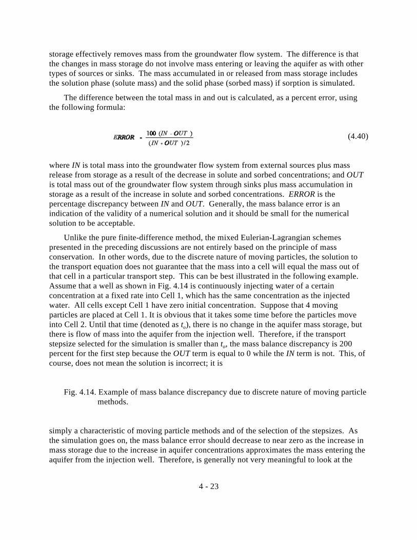
4 - 23
storage effectively removes mass from the groundwater flow system. The difference is thatthe changes in mass storage do not involve mass entering or leaving the aquifer as with othertypes of sources or sinks. The mass accumulated in or released from mass storage includesthe solution phase (solute mass) and the solid phase (sorbed mass) if sorption is simulated.
The difference between the total mass in and out is calculated, as a percent error, usingthe following formula:
(4.40)
where IN is total mass into the groundwater flow system from external sources plus massrelease from storage as a result of the decrease in solute and sorbed concentrations; and OUTis total mass out of the groundwater flow system through sinks plus mass accumulation instorage as a result of the increase in solute and sorbed concentrations. ERROR is thepercentage discrepancy between IN and OUT. Generally, the mass balance error is anindication of the validity of a numerical solution and it should be small for the numericalsolution to be acceptable.
Unlike the pure finite-difference method, the mixed Eulerian-Lagrangian schemespresented in the preceding discussions are not entirely based on the principle of massconservation. In other words, due to the discrete nature of moving particles, the solution tothe transport equation does not guarantee that the mass into a cell will equal the mass out ofthat cell in a particular transport step. This can be best illustrated in the following example. Assume that a well as shown in Fig. 4.14 is continuously injecting water of a certainconcentration at a fixed rate into Cell 1, which has the same concentration as the injectedwater. All cells except Cell 1 have zero initial concentration. Suppose that 4 movingparticles are placed at Cell 1. It is obvious that it takes some time before the particles moveinto Cell 2. Until that time (denoted as t ), there is no change in the aquifer mass storage, buto
there is flow of mass into the aquifer from the injection well. Therefore, if the transportstepsize selected for the simulation is smaller than t , the mass balance discrepancy is 200o
percent for the first step because the OUT term is equal to 0 while the IN term is not. This, ofcourse, does not mean the solution is incorrect; it is
Fig. 4.14. Example of mass balance discrepancy due to discrete nature of moving particle methods.
simply a characteristic of moving particle methods and of the selection of the stepsizes. Asthe simulation goes on, the mass balance error should decrease to near zero as the increase inmass storage due to the increase in aquifer concentrations approximates the mass entering theaquifer from the injection well. Therefore, is generally not very meaningful to look at the

4 - 24
mass balance at a particular step with moving particle methods; rather, it is the averaged andaccumulated mass balance information that is more indicative of the overall acceptability ofthe simulation.
The mixed Eulerian-Lagrangian solution schemes implemented in the MT3D transportmodel provides many options which can be adjusted to achieve minimal mass balancediscrepancy. These options include the number and initial distribution pattern of movingparticles, different particle tracking schemes, and the selection of optimal stepsizes.
4.8 A Note on the Pure Finite-Difference Method
The pure finite-difference method solves all terms in the transport equation using thefinite-difference scheme. The word "pure" is used to distinguish it from the mixed Eulerian-Lagrangian method utilized in the MT3D transport model which solves the advection termusing one of the method-of-characteristics schemes and the other terms using the finite-difference scheme. The pure finite-difference method can lead to significant numericaldispersion for problems having very sharp concentration fronts. However, because the purefinite-difference method does not involve any particle tracking calculation or concentrationinterpolation, it is normally more efficient computationally. Furthermore, because the finite-difference method is entirely based on the principle of mass conservation, it should have verysmall mass balance discrepancy at every step. For these reasons, a finite-difference routinehas also been provided in the MT3D model to supplement the MOC, MMOC or HMOCscheme for solving the advection term.
The finite-difference routine solves the unexpanded advection term and the sink/sourcedirectly based on an upstream weighting scheme as given below:
(4.41)
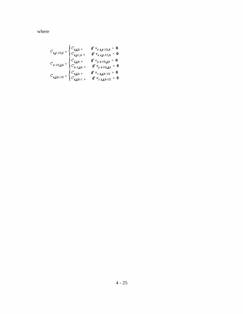
4 - 25
where

5 - 1
Chapter 5PROGRAM STRUCTURE AND DESIGN
5.1 OVERALL STRUCTURE
The computer program of the MT3D transport model uses a modular structure similar tothat implemented in the U. S. Geological Survey modular three-dimensional finite-differencegroundwater flow model, or MODFLOW, (McDonald and Harbaugh, 1988). Like theMODFLOW model, the MT3D model consists of a main program and a large number ofhighly independent subroutines, called modules, which are grouped into a series of"packages". Each of these packages deals with a single aspect of the transport simulation. The similarity between MT3D and MODFLOW in the program structure and design isintended to facilitate the use of the MT3D transport model in conjunction with MODFLOW,one of the more widely used flow models.
The general procedures performed in the transport model for a typical simulation run areillustrated in Fig. 5.1. The simulation time is divided into "stress periods", also referred to as"pumping periods", within which the stress (i.e., the sink/source) parameters are constant. Each stress period, in turn, is divided into a series of time steps. The hydraulic heads andfluxes at each time step are solved by the flow model and used by the transport model. Sincethe flow equation is generally solved using an implicit interactive method whereas thetransport equation is solved in the MT3D model with an explicit direct method, the length ofeach time step for the head solution may exceed the limitation required for stability in thetransport solution. Thus, each time step used in obtaining the head solution is further dividedinto a number of smaller time increments, termed transport steps, within which the hydraulicheads and fluxes are assumed to be constant.
Fig. 5.1. General procedures for a typical transport simulation.
Prior to entering the stress period loop, the program executes three procedures whichpertain to the simulation as a whole (see Fig.5.1). In the Define procedure, the simulationproblem is defined; that is, the size of the model, the number of stress periods, and the varioustransport options to be used in the simulation are specified. In the Allocate procedure,computer memory is allocated for the data arrays whose dimensions depend on the parametersspecified in the Define procedure. In the Read & Prepare procedure, input data that areconstant throughout the simulation are read and processed. These input data include spatialand temporal discretization information, boundary conditions, initial conditions, transportparameters, solution parameters, and output control options.
5 - 2
The first procedure within the stress period loop is the Stress procedure which obtainstiming information for the current stress period: the length of the stress period, the number oftime steps within the stress period, and the length of each time step. A second Read &Prepare procedure then reads and prepares input data which are constant within the currentstress period, i.e., the concentrations of those sources or sinks that need to be specified. Thetransport model obtains the location, type, and flow rates of all sources and sinks simulated inthe flow model from an unformatted head and flow file saved by the flow model. Sourceconcentrations are automatically set equal to zero unless the user specifies a differentconcentration through this Read & Prepare procedure. Sink concentrations are always setequal to the concentration in the aquifer at the sink location, except for evapotranspiration,whose concentration can be specified through this Read & Prepare procedure.
Within the time step loop, A third Read & Prepare procedure reads and processes thehydraulic heads and flow terms saved by the flow model, automatically incorporating thespecified hydrologic boundary conditions. The Coefficient procedure then calculates certaincoefficients that are constant within each time step of the head solution, such as the dispersioncoefficient.
The transport step loop contains four procedures. The Advance procedure determines anappropriate stepsize for use in the current transport step. The Solve procedure solves each transport component with an explicit mixed Eulerian-Lagrangian solution scheme andcalculates the mass into or out of the aquifer through each component. The Budget procedurecalculates and prepares global mass balance information; and the Output procedure prints orsaves simulation results as needed according to the user-specified output control options.
The general procedures outlined in the preceding discussion are implemented for each ofthe four components in the transport equation: advection, dispersion, sink/source mixing, andchemical reactions. The implementation is done through the use of individual modules, orhighly independent subroutines, each of which performs one particular procedure. Forexample, the advection component is implemented through 3 modules, named ADV1AL,ADV1RP, and ADV1SV, respectively, where ADV indicates the transport component(advection) for which these modules are implemented. The number (1) indicates the currentversion number of the computer code. AL (abbreviation for Allocate) , RP (abbreviation forRead & Prepare), and SV (abbreviation for Solve) indicate the procedures these modulesperform. These modules, which are called by the main program, are termed primary modulesto distinguish them from secondary modules, which are used only inside the primary modulesto which they belong. The primary modules ADV1AL, ADV1RP, and ADV1SV and theirassociated secondary modules are grouped into a "package", called the Advection Package(abbreviated as ADV) (see Fig. 5.2). Dispersion, sink/source mixing, and chemical reactionsare similarly implemented and grouped into the Dispersion Package (DSP), Sink & SourceMixing Package (SSM), and Chemical Reaction Package (RC7).
In addition to the four transport component packages, the MT3D model program includesthree additional packages: the Basic Transport Package (BTN), the Flow Model InterfacePackage (FMI), and the Utility Package (UTL). The Basic Transport Package handles basic
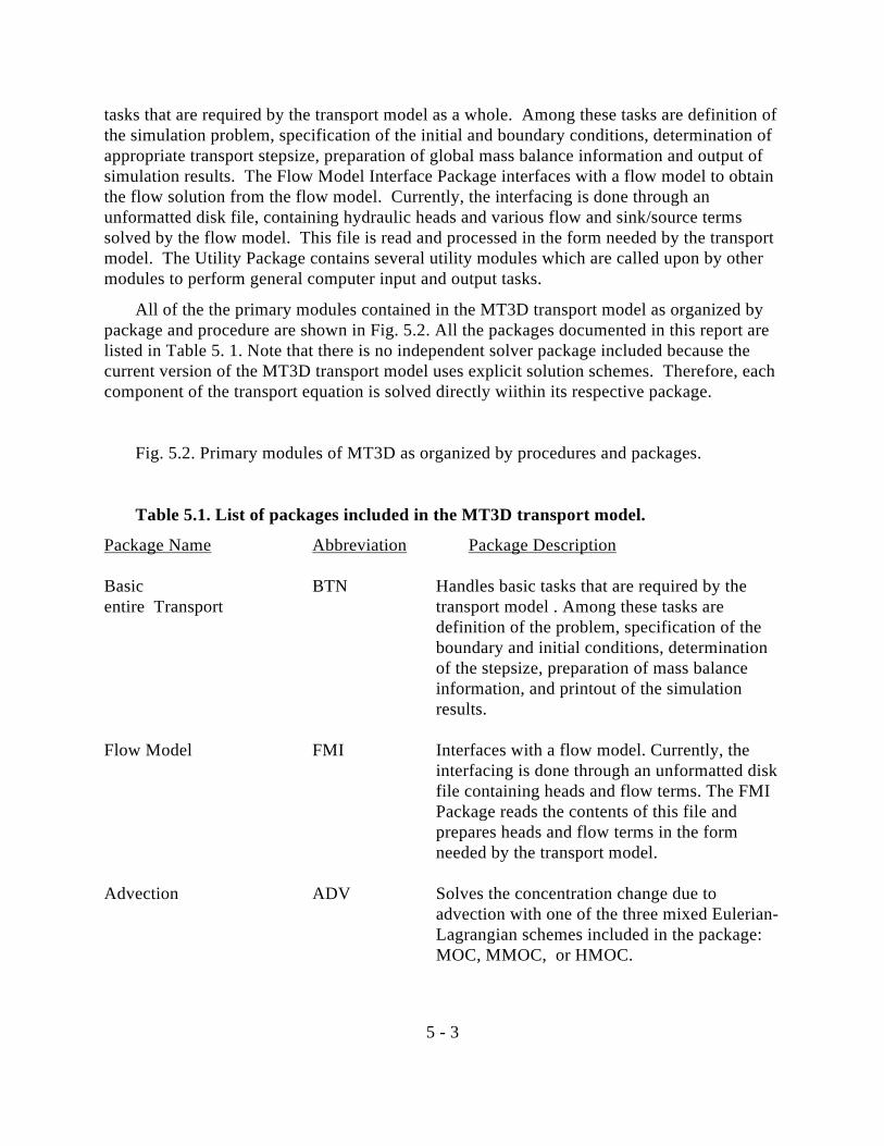
5 - 3
tasks that are required by the transport model as a whole. Among these tasks are definition ofthe simulation problem, specification of the initial and boundary conditions, determination ofappropriate transport stepsize, preparation of global mass balance information and output ofsimulation results. The Flow Model Interface Package interfaces with a flow model to obtainthe flow solution from the flow model. Currently, the interfacing is done through anunformatted disk file, containing hydraulic heads and various flow and sink/source termssolved by the flow model. This file is read and processed in the form needed by the transportmodel. The Utility Package contains several utility modules which are called upon by othermodules to perform general computer input and output tasks.
All of the the primary modules contained in the MT3D transport model as organized bypackage and procedure are shown in Fig. 5.2. All the packages documented in this report arelisted in Table 5. 1. Note that there is no independent solver package included because thecurrent version of the MT3D transport model uses explicit solution schemes. Therefore, eachcomponent of the transport equation is solved directly wiithin its respective package.
Fig. 5.2. Primary modules of MT3D as organized by procedures and packages.
Table 5.1. List of packages included in the MT3D transport model.
Package Name Abbreviation Package Description
Basic BTN Handles basic tasks that are required by theentire Transport transport model . Among these tasks are
definition of the problem, specification of theboundary and initial conditions, determinationof the stepsize, preparation of mass balanceinformation, and printout of the simulationresults.
Flow Model FMI Interfaces with a flow model. Currently, the interfacing is done through an unformatted diskfile containing heads and flow terms. The FMIPackage reads the contents of this file andprepares heads and flow terms in the formneeded by the transport model.
Advection ADV Solves the concentration change due toadvection with one of the three mixed Eulerian-Lagrangian schemes included in the package:MOC, MMOC, or HMOC.

5 - 4
Dispersion DSP Solves the concentration change due todispersion with the explicit finite differencemethod.
Sink & Source SSM Solves the concentration change due to fluid Mixing sink/source mixing with the explicit finite
difference method. Sink/source terms mayinclude wells, drains, rivers, recharge andevapotranspiration. The constant-headboundary and general-head-dependentboundary are also handled as sink/source termsin the transport model.
Chemical RCT Solves the concentration change due tochemical Reactions reactions. Currently, the chemical reactions
include linear or nonlinear sorption isothermsand first-order irreversible rate reactions(radioactive decay or biodegradation).
Utility UTL Contains a number of utility modules that arecalled upon by primary modules to performsuch general-purposed tasks as input/output ofdata arrays.
5.2 MEMORY ALLOCATION
The main computer memory required to run the MT3D model is allocated at programexecution time in two one-dimensional storage arrays called the "X" array for real variablesand the "IX" array for integer variables. The real X and integer IX arrays are then partitionedto store individual date arrays whose dimensions depend on the problems to be simulated. The sizes of individual arrays are calculated and accumulated by the Allocate procedure oftheir respective packages; the accumulated sizes serve as pointers indicating the locations ofindividual arrays within the X or IX array. If the accumulated sizes of the individual arraysexceed the length of the X or IX array which is preset at program compilation, programexecution stops. If this happens, the length of the X or IX array must be increased bymodifying the following parameter statement in the main program:
PARAMETER (LENX=450000, LENIX=36000)
where LENX is the length of the X array and LENIX the length of the IX array. Thelengths of the X and IX arrays required for a specific problem depend on the type and numberof packages used. The length of the X array will generally range from 10 to 30 times the
5 - 5
number of cells in the grid plus 4 times the maximum number of moving particles allowed;the length for the IX array is approximately 2 to 4 times the number of cells. The exact sizesof the X and IX arrays can be calculated according to the instructions in Appendix A. Theycan also be known by simply running the program, which will print out the required X and IXsizes before it stops execution if either one or both of these arrays are dimensioned too small.
The MT3D model program is written for three-dimensional simulation. When theprogram is used for one- or two-dimensional applications, some arrays are not needed and tosave memory storage, these arrays are not allocated space in the X or IX array. For example,array QZ is intended for storing fluxes between vertical layers. If the program is used tosimulate a two-dimensional problem in plan view, QZ is not needed and thus is not allocatedstorage space; and as a result, it is never used, or operated upon, in any way in the program. This is important to keep in mind when the user wants to modify the computer code.
5.3 INPUT STRUCTURE
The input structure of the model program is designed to gather input data from as manydifferent files as needed in a simulation. This structure is similar in many ways to that ofMODFLOW. Therefore, the users who are familiar with MODFLOW should find it very easyand straightforward to prepare input for the MT3D model.
The Basic Transport Package is always used in every simulation. Thus, an input file forthe Basic Transport Package is required every time the program is run. In the input file to theBasic Transport Package, there is a record containing the logical TRNOP array. Each elementof the TRNOP array corresponds to a major option, generally a package (see Fig. 5.3). Anoption is invoked by setting the value of its corresponding TRNOP element to T (for True),and turned off by setting the value to F (for False). When an option is used, an input filecontaining data exclusively for that option is then required. For example, the second elementof the TRNOP array corresponds to the Dispersion Option (or Package). If it is necessary tosimulate dispersion, the second TRNOP array element must be entered as T. An input filecontaining dispersion parameters must be created and read by the program.
In addition to the main input file for the Basic Transport Package and the input files forthe various transport component packages which are used, the transport model alwaysrequires another input file which contains hydraulic heads, fluxes across cell interfaces, andthe location and flow rate of sinks and/or sources. This file is generated by a flow model usedin conjunction with the transport model, and read by the Flow Model Interface Package of theMT3D model. The structure and form of this file are discussed in Chapter 6.
In the standard ANSI FORTRAN 77 language, a data file must be opened with aFORTRAN unit number and a file name before it can be accessed by the program. This isdone in the subroutine OPENFL which is included in the Utility Package. The file names canbe entered interactively from the monitor screen or through a response file in a batch mode as
5 - 6
discussed in the next chapter. The unit numbers associated with major input files are preset inthe main program. They can be changed, if necessary, by modifying the following parameterstatement in the main program:
PARAMETER (INBTN=l,INADV=2,INDSP=3,INSSM=4,INRCT=9,INUHF=10)
where
INBTN is the unit number for the Basic Transport Package;
INADV is the unit number for the Advection Package;
INDSP is the unit number for the Dispersion Package;
INSSM is the unit number for the Sink & Source Mixing Package;
INRCT is the unit number for the Chemical Reaction Package; and
INUHF is the unit number for the unformatted head & flow file, read by the FlowModel Interface Package.
Once the unit number associated with a package is used in the simulation, it must not beused again elsewhere.
5.4 OUTPUT STRUCTURE
The program generates a standard output file and several optional output files. Thestandard output file is generated every time the model is run. The optional output files aregenerated only if they are requested. The amount, type, and frequency of information to bewritten on the output files are controlled by the user-specified options in the input file to theBasic Transport Package. The functions of these output files are listed below:
1. The Standard Output File: contains echo of input data to ensure they are read in properly, printout of simulated concentrations, and some other essential informationsuch as model-calculated parameters and mass budget at user-specified times and atthe end of the simulation.
2 . The Unformatted Concentration File (default name: MT3D.UCN): containsconcentrations saved at user-selected times in the unformatted form for acontinuation run or for post-processing purposes.
3. The Observation Point File (default name: NMD.OBS): contains concentrationsversus total elapsed time at user-specified observation points at every transport step.
4. The Mass Balance Summary File (default name: MT3D.MAS): contains a one-linesummary of mass budget at every transport step for checking purposes.

5 - 7
5. The Model Grid Configuration File (default name: MT3D.CNF): contains modelspatial discretization information to be used by the post-processor for graphicpresentation.
The unit numbers associated with these output files are preset in the following parameterstatement in the main program:
PARAMETER (IOUT=ll, IUCN=12, IOBS=13, IMAS=14, IUCN=15)
where
IOUT istheunitnumberfortheStandardOutputFile;
IUCN is the unit number for the Unfonnatted Concentration File, MT3D.UCN;
IOBS is the unit number for the Observation Point File, MT3D.OBS;
IMAS is the unit number for the Mass Balance Summary File, MT3D.MAS;
ICNF is the unit number for the Model Grid Configuration File, MT3D.CNF.
These unit numbers can be changed, ff necessary, by modifying the above parameterstatement.
5.5 COMPUTER PROGRAM DESCRIPTION
The computer program of the MT3D transport model is written in the standardFORTRAN 77 language as defined by the American National Standards Institute (ANSI). Tomaximize the portability of the computer program, only language features pertaining to theANSI standard are used except the IMPLICIT NONE statement. The use of this statementrequires the explicit declaration of all variables' types and is extremely helpful in preventingvariable names from being misspelled, a common error in writing or modifying programs. Ifthe compiler the user has does not support this extension, the IMPLICIT NONE statement inall subroutines should be commented out. Furthermore, all real variables in the program aredeclared as single precision. If it is necessary to run the model in double precision, modify allstatements starting with REAL * 4 in each subroutine to REAL * 8.
The main program and all subroutines of the MT3D program (including primary andsecondary modules) are described briefly in the following sections. For more information, theuser may refer to the extensively commented source code included in the disk and listed inAppendix F.

5 - 8
5.5.1 Main Program -- MTMAIN
The main program controls the overall execution of the entire program. A flow chartshowing all the primary modules called by the main program is provided in Fig. 5.4. Thebasic steps of the main program for each simulation are:
1. Set the lengths of the X and DC arrays.
2. Assign unit numbers to major input and output files and open these files.
3. Define the simulation problem in terms of layers, rows, columns, stress periods, andmajor transport options to be used.
4. Allocate space in the X and IX arrays for all individual data arrays.
5 . If either X or IX array is not dimensioned large enough, stop.
6 . Read and process input data which are constant throughout the simulation.
7 . For each stress period:
(a) Obtain stress period timing information.
(b) Read and process the concentrations of sources or sinks that need to be specified.
(c) For each time step:
(1) Read hydraulic heads, fluxes across cell interfaces, and the locations and flowrates of sinks or sources.
(2) Calculate coefficients that are constant within the current dm step.
(3) For each transport step:
(i) Determine an appropriate stepsize for the current transport step.
(ii) Solve each component of the transport equation.
(iii) Prepare mass balance information.
(iv) Print or save simulation results.
(v) If the number of transport steps exceeds the specified maximum, stop.
8. End program.
Fig. 5.4. Flow chart for the main program showing all modules.

5 - 9
5.5.2 Basic Transport Package -- MTBTNI
The Basic Transport Package consists of eight primary modules, each of which isdescribed below in the order of execution:
BTNLDF Define the simulation problem by reading the number of layers, rows, columnsand stress periods as well as the transport options to be used;
BTNLAL Allocate space for basic data arrays needed by the model as a whole;BTNLRP Read and prepare basic data arrays used by the entire model;BTNLST Read stress period timing information;BTNLAD Determine an appropriate stepsize for each transport step;BTNLSV Update cell concentrations and prepare for simulation of the next step;BTNLBD Prepare global mass balance information;BTN10T Print or save simulation results according to the user-specified options.
5.5.3 Flow Model Interface Package -- MTFMI]
The Flow Model Interface Package consists of two primary modules and three secondarymodules:
FM11RP1 Read and prepare hydraulic heads and fluxes across cell interfaces in thecolumn, row and layer directions on a cell-by-cell basis by calling secondarymodule READHQ.
FM11RP2 Read and prepare the locations and flow rates of the various sink/source termsby calling secondary modules READPS (for reading point sinks or sources) andREADDS (for reading areally distributed sinks or sources).
5.5.4 Advection Package -- MTADVI
The Advection Package consists of three primary modules and a number of secondarymodules:
ADVLAL Allocate space for data arrays needed by the Advection Package;ADVLRP Read and prepare input data needed for solving the advection term;ADVISV Solve the advection term. This primary module includes the following
secondary modules, which are named according to the function they perform:LOCATE: Find cell indices (J,I,K) of a particle located at coordinates (x,y,z);VPOINT: Interpolate particle velocity at an arbitrary point based on the
piecewise linear scheme;EULER: Perform particle tracking with the first-order Euler algorithm;RK4: Perform particle tracking with the fourth-order Runge-Kutta
algorithm;

5 - 10
PARMGR: Manage the distribution of moving particles dynamically, insertingor deleting particles as necessary;
CNGRAD: Calculate relative concentration gradient of a cell with itsneighboring cells;
GENPTN: Insert particles in a finite-difference cell according to fixedpatterns;GENPTR: Insert particles in a finite-difference cell randomly;CPOINT. Calculate concentration at an arbitrary point from neighboring
nodes with the first-order polynomial interpolation;QCFLUX Compute mass flux into or out of a finite-difference cell based on
finite-difference formulation.
5.5.5 Dispersion Package -- MTDSPI
The Dispersion Package consists of four primary modules, each of which is describedbelow in the order of execution:
DSPLAL Allocate space for data arrays needed by the Dispersion Package;DSPLRP Read and prepare dispersion parameters;DSPLCF Calculate components of the hydrodynamic dispersion coefficient;DSPI SV Solve the dispersion term using the explicit finite difference
formulation;
5.5.6 Sink & Source Mixing Package -- MTSSMI
The Sink & Source Mixing Package consists of three primary modules, each of which isdescribed below in the order of execution:
SSM1AL Allocate space for data arrays needed by the Sink & Source MixingPackage;
SSM1RP Read and prepare concentrations of sources and/or sinks that need tobe specified;
SSM1SV Solve the concentration change due to sink/source mixing using theexplicit finite difference formulation.
5 - 11
5.5.7 Chemical Reaction Package -- MTRCTI
The Chemical Reaction Package consists of three primary modules and a secondarymodule:
RCT1AL Allocate space for data arrays needed by the Chemical ReactionPackage;
RCT1RP Read and prepare chemical reaction parameters;RCT1SV Solve the concentration change due to chemical reactions using the
explicit finite difference formulation.Both RCTLRP and RCTLSV use the following secondary module:
RFCOEF: Calculate retardation factor for linear or non-linearsorption isotherms.
5.5.8 Utility Package -- MTUTLI
The Utility Package consists of the following utility subroutines called upon by othermodules to perform general computer input/output tasks:
OPENFL Open an input or output file;RARRAY Read a one- or two-dimensional REAL data array using the block,
zonal, list-directed, unformatted, or any user-specified format;IARRAY Read a one- or two-dimensional INTEGER data array with the
block, zonal, list-directed, unformatted, or any user-specified format;RPRINT Print a one- or two-dimensional REAL data array with the wrap or
strip format;IPRINT Print a one- or two-dimensional INTEGER data array with the wrap
or strip format.

6 - 1
Chapter 6INPUT INSTRUCTIONS
6.1 GENERAL INFORMATION
The MT3D model program uses a combination of formatted, list-directed andunformatted input forms, and calls two general array readers to enter data arrays. These inputforms and the array readers are described in this section for easy reference in the preparationof input files.
6.1.1 Input Forms
Formatted
If an input value is entered using the formatted form, the type of value and the space itoccupies must agree with its format specifier. Four types of input variables are used in theprogram: Integer, Real, Character and Logical.
In the input instructions to be followed, the format specifier for integer variables iswritten as Iw where I implies that the variable must have the form of an integer (it must notcontain a decimal point or exponent); and w is the number of spaces reserved for the variable. If the input value is less than w spaces wide, the unoccupied spaces are treated as blanks bydefault. It is always good practice to enter the value right-justified.
The format specifier for real variables is written as Fw.d where w is the number of spacesreserved for the entire input value, with the fractional part taking d spaces. When a decimalpoint is present, it overrides the d specified in the format. Thus, even though the specifier forreal variables is written as F10.0 in the input instructions, input values can be entered insuch forms as 12.345 or 0.12345. Furthermore, input values in the exponential form, suchas 1.2345E-5, are also acceptable.
The format specifier for the character variable is written as Aw where w is the number ofspaces reserved for the character variable. If the character string is less than w characterswide, unfilled spaces are treated as blanks.
Finally, the format specifier for the logical variables is written as Lw where w is thenumber of spaces reserved for the logical variable. The logical variable must be enteredeither as T (for True) or as F (for False), leaving unoccupied spaces blank.
List-Directed
List-directed input (also referred to as free format) has several characteristics: (1) a list-directed record is a sequence of values separated by either commas or blanks with multipleblanks allowed; (2) a list-directed record terminates when the number of the input values
6 - 2
equals the number of items in the input list or until a slash (/) is encountered; (3) a list-directed record may occupy several lines of an input file, but each new record should start at anew line; and finally, (4) list-directed input permits the use of a repeat count in the form,
n*d
where n is an unsigned-nonzero integer constant, and the input n*d causes n consecutivevalues of d to be entered.
Unformatted
An unformatted file is a sequence of unformatted records in the form of binary characters. An unformatted file cannot be visually examined, but is smaller in size and faster to processthan a formatted file. The model program uses the unformatted form to enter the hydraulicheads and flow terms saved by a flow model.
6.1.2 Array Readers RARRAY and IARRAY
Most of the input data to be entered to the model by the user will consist of one- or two-dimensional real or integer arrays. Three-dimensional arrays are treated as a series of two-dimensional arrays, each of which corresponds to an individual model layer and is entered insequence according to the layer number.
In the MT3D model, arrays are entered as an "array-control record", plus, optionally, aseries of records containing the array elements. If all the elements of an array have the samevalue, the value is specified on the control record and it is not necessary to read the associatedarray. If the array elements vary, records containing the array values are read using thevarious input forms as specified on the array-control record. To perform these tasks, twoutility subroutines, RARRAY for reading one- or two-dimensional real arrays, and IARRAYfor reading one- or two-dimensional integer arrays, are provided in the program. These twoarray readers are compatible to array readers U2DREL and U2DINT provided in theMODFLOW model (McDonald and Harbaugh, 1988). However, RARRAY and IARRAYalso permit the input of array values by block, zonal and list-directed (or free) formats.
For each array to be entered, RARRAY or IARRAY reads an array-control record firston the unit reserved for the major option which calls the array reader. For example, unit 1 ispreset for the Basic Transport Package, thus, RARRAY or IARRAY reads the array-controlrecord in the input file for the Basic Transport Package from unit 1. The content and form ofthe array control record are as follows:
FOR REAL ARRAY READER (RARRAY):
Record: IREAD CNSTNT FMTIN IPRNFormat: I10 F10.0 A20 I10
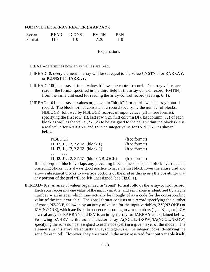
6 - 3
FOR INTEGER ARRAY READER (IAARRAY):
Record: IREAD ICONST FMTIN IPRNFormat: I10 I10 A20 I10
Explanations
IREAD--determines how array values are read.
If IREAD=0, every element in array will be set equal to the value CNSTNT for RARRAY,or ICONST for IARRAY.
If IREAD=100, an array of input values follows the control record. The array values areread in the format specified in the third field of the array-control record (FMTIN),from the same unit used for reading the array-control record (see Fig. 6. 1).
If IREAD=101, an array of values organized in "block" format follows the array-controlrecord. The block format consists of a record specifying the number of blocks,NBLOCK, followed by NBLOCK records of input values (all in free format),specifying the first row (Il), last row (I2), first column (Jl), last column (J2) of eachblock as well as the value (ZZ/IZ) to be assigned to the cells within the block (ZZ isa real value for RARRAY and IZ is an integer value for IARRAY), as shownbelow:
NBLOCK (free format)I1, I2, J1, J2, ZZ/IZ (block 1) (free format)I1, I2, J1, J2, ZZ/IZ (block 2) (free format). . . . . . . .I1, I2, J1, J2, ZZ/IZ (block NBLOCK) (free format)
If a subsequent block overlaps any preceding blocks, the subsequent block overrides thepreceding blocks. It is always good practice to have the first block cover the entire grid andallow subsequent blocks to override portions of the grid as this averts the possibility thatany portion of the grid will be left unassigned (see Fig.6. 1).
If IREAD=102, an array of values organized in "zonal" format follows the array-control record.Each zone represents one value of the input variable, and each zone is identified by a zonenumber -- an integer which may actually be thought of as a code for the correspondingvalue of the input variable. The zonal format consists of a record specifying the numberof zones, NZONE, followed by an array of values for the input variables, ZV(NZONE) orIZV(NZONE), which are listed in sequence according to zone numbers (1, 2, 3, ..., etc); ZVis a real array for RARRAY and IZV is an integer array for IARRAY as explained below.Following ZV/IZV is the zone indicator array A(NCOL,NROW)/IA(NCOL,NROW)specifying the zone number assigned to each node (cell) in a given layer of the model. Theelements in this array are actually always integers, i.e., the integer codes identifying thezone for each cell. However, they are stored in the array reserved for input variable itself,

6 - 4
and thus follow the format of the input variable. Hence, the zone indicators are read usingthe format as specified in the third field of the array-control record (FMTIN) which mustbe a real format specifier for RARRAY and an integer format specifier for IARRAY. If thezone indicator for a cell is equal to zero, the value for that cell is set to zero (see Fig. 6. 1).
The zonal format for RARRAY:
NZONES (free format)ZV(l),.ZV(2).......... ZV(NZONE) (free format)A(NCOL,NROW) (using format FMTIN)
The zonal format for IARRAY:
NZONE (free format)IZV(l), IZV(2)........ IZV(NZONE) (free format)IA(NCOL,NROW) (using format FMTIN)
If IREAD=103, an array of values follows the array-control record. The array values are
read using list-directed or free format (see Fig. 6. 1).
If IREAD=any value other than 0, 100, 101, 102, and 103, array values are read from aseparate file.
If IREAD>O, it is the unit number on which the external file is read using the formatspecified in FMTIN.
If IREAD<O, the absolute value of IREAD gives the unit number on which the arrayvalues are read from an external unformatted file. The unformatted filecontains one dummy record, followed by an unformatted record ofNCOL*NROW values.
CNST'NT/ICONST--is a constant. Its use depends of the value of IREAD.
If IREAD=0,every element in the array is set equal to CNSTNT/ICONST.
If IREAD…0, and CNSTNT/ICONST…0, elements in the array are multiplied byCNSTNT/ICONST.
FMTIN--is the format specifier used to read array values or the zonal indicator array. Theformat must be enclosed in parentheses; for example, (15F5.0) for real values and(15I5) for integer input values.
IPRN--is a flag indicating whether the array being read should be printed out for checkingand also serves as a code indicating the format that should be used in printing. It isused only if IREAD is not equal to zero. IPRN is set to zero if the specified valueexceeds those defined in Table 6.1 as shown below. If IPRN is less than zero, thearray will not be printed.

6 - 5
Table 6.1. Printing formats corresponding to the EPRN code.
(After McDonald and Harbaugh, 1988)
IPRN RARRAY IARRAY
0 10G11.4 10I111 11G10.3 60Il2 9G13.6 40I23 l5F7.1 30I34 15F7.2 25I45 15F7.3 20156 15F7.47 20F5.08 20F5.19 20F5.2
10 20F5.311 20F5.412 l0G11.4
CNSTNT FMTIN IRPNIREAD
100 0. (l0F5.1) 32.1 2.1 2.1 2.1 2.1 2.1 2.1 2.1 2.1 2.12.1 2.1 2.1 2.1 2.1 2.1 2.1 2.1 2.1 2.1
10.2 10.2 10.2 10.2 10.2 10.2 10.2 10.2 10.2 10.210.2 10.2 10.2 10.2 10.2 10.2 10.2 10.2 10.2 10.223.5 23.5 23.5 23.5 23.5 23.5 23.5 0.4 0.4 0.423.5 23.5 23.5 23.5 23.5 23.5 23.5 0.4 0.4 0.423.5 23.5 23.5 23.5 23.5 23.5 23.5 0.4 0.4 0.423.5 23.5 23.5 23.5 23.5 23.5 23.5 0.4 0.4 0.423.5 23.5 23.5 23.5 23.5 23.5 23.5 0.4 0.4 0.4
0 0 0 0 0 0 0 0.4 0.4 0.4
(a) An array of 10 x 10 is read with the user-specified format (l0F5.1) (IREAD= 100).
101 0. (FMTIN not used) 35 <------------- NBLOCK
1 10 1 10 0
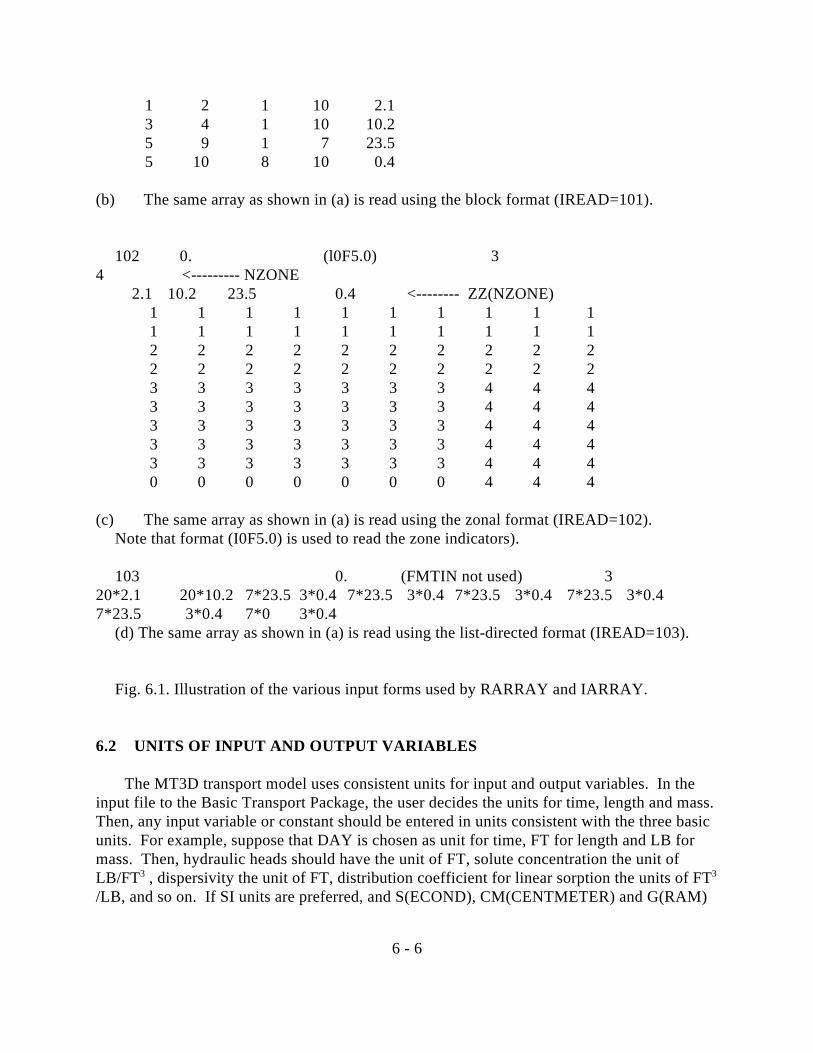
6 - 6
1 2 1 10 2.13 4 1 10 10.25 9 1 7 23.55 10 8 10 0.4
(b) The same array as shown in (a) is read using the block format (IREAD=101).
102 0. (l0F5.0) 34 <--------- NZONE
2.1 10.2 23.5 0.4 <-------- ZZ(NZONE)1 1 1 1 1 1 1 1 1 11 1 1 1 1 1 1 1 1 12 2 2 2 2 2 2 2 2 22 2 2 2 2 2 2 2 2 23 3 3 3 3 3 3 4 4 43 3 3 3 3 3 3 4 4 43 3 3 3 3 3 3 4 4 43 3 3 3 3 3 3 4 4 43 3 3 3 3 3 3 4 4 40 0 0 0 0 0 0 4 4 4
(c) The same array as shown in (a) is read using the zonal format (IREAD=102).Note that format (I0F5.0) is used to read the zone indicators).
103 0. (FMTIN not used) 320*2.1 20*10.2 7*23.5 3*0.4 7*23.5 3*0.4 7*23.5 3*0.4 7*23.5 3*0.47*23.5 3*0.4 7*0 3*0.4
(d) The same array as shown in (a) is read using the list-directed format (IREAD=103).
Fig. 6.1. Illustration of the various input forms used by RARRAY and IARRAY.
6.2 UNITS OF INPUT AND OUTPUT VARIABLES
The MT3D transport model uses consistent units for input and output variables. In theinput file to the Basic Transport Package, the user decides the units for time, length and mass. Then, any input variable or constant should be entered in units consistent with the three basicunits. For example, suppose that DAY is chosen as unit for time, FT for length and LB formass. Then, hydraulic heads should have the unit of FT, solute concentration the unit ofLB/FT , dispersivity the unit of FT, distribution coefficient for linear sorption the units of FT3 3
/LB, and so on. If SI units are preferred, and S(ECOND), CM(CENTMETER) and G(RAM)

6 - 7
are selected as the units for time, length and mass, respectively, then, heads should have theunit of CM, concentration the units of G/CM , dispersivity the unit of CM, distribution3
coefficient for linear sorption the units of CM /G, and so on.3
A special note on the unit for concentration. Sometimes, it is more convenient to workwith relative concentration. In that case, all concentrations input into the model can be scaledaccording to the maximum concentration (Co) of either aquifer or fluid sources. Subsequently, the model simulates the changes in the relative concentration (C/Co).
It should be emphasized that the unit names entered are used for identification purposesonly, and do not affect the model simulation results in any way.
6.3 INTERFACE WITH THE FLOW MODEL
MT3D is designed to be used in conjunction with a block-centered finite-differenceflowmodel. This allows the user to construct and calibrate a flow model independently. Priorto running MT3D, the heads, fluxes across cell interfaces in all directions, and locations andflow rates of the various sinks/sources, as solved by the flow model, should be saved in anunforrnatted head and flow file. This file should be saved in such a way that it can beretrieved by MT3D correctly through the Flow Model Interface Package. Appendix B,Linking MT3D with a Flow Model, gives more detailed information on the structure and formof the unformatted head and flow file.
In many cases, the U. S. Geological Survey modular three-dimensional finite-differencegroundwater flow model (MODFLOW) will be used for the head solution; a package hastherefore been written for use with MODFLOW to save heads and flow terms needed byMT3D. T'he package is named LKMT and included in the disk labelled Flow Model, whichcontains a version of the MODFLOW program already incorporating the LKMT package. Ifit is preferred to use a version of MODFLOW other than the one included in the Flow Modeldisk, do the followmg to add the LKMT package mto MODFLOW:
1. Insert the statements in file LKMT.INC into the MODFLOW main program betweenthe following two statements:
CALL BAS10C (... )
IF(CNVG .EQ. 0) STOP
and recompile the main program. Then, compile file LKMT.FOR and link it with therest of the MODFLOW files. Both files LKMT.INC and LKMT.FOR are included inthe Flow Model Disk.
2. Insert a positive integer number in the 22 element of the IUNIT array in the input nd
file for the MODFLOW Basic Package. This instructs the MODFLOW program tosave the unformatted heads and flow terms for use in MT3D. It also serves as the

6 - 8
unit number on which the heads and flow terms will be saved. If the IUNIT(22) isentered as zero, no file will be saved by the LKMT Package.
It should be pointed out that the MODFLOW program already has the option to saveheads andcell-by-cell flow terms in unformatted files. However, the MODFLOW programdoes not calculate fluxes between constant-head cells, which are required in the MT3Dtransport model. Furthermore, the MODFLOW program writes all the sink/source termsusing three-dimensional arrays, thereby taking larger disk space than necessary. For thesereasons, the MT3D program does not use the unformatted flow and cell-by-cell flow files inthe forms saved by invoking the MODFLOW output control options.
6.4 INPUT INSTRUCTIONS FOR THE BASIC TRANSPORT PACKAGE
Input to the Basic Transport Package is read on unit 1, which is preset in the mainprogram. Since the BTN Package is needed for every simulation, this input file is alwaysrequired.
FOR EACH SIMULATION:A1 Record: HEADNG(1)
Format: A80HEADNG(1) is the first line of any title or heading for the simulation run. Theline should not be longer than 80 characters.
A2 Record: HEADNG(2)Format: A80HEADNG(2) is the second line of any title or heading for the simulation run. Theline should not be longer than 80 characters.
A3 Record: NLAY, NROW, NCOL, NPERFormat: 4110NLAY is the total number of layers;NROW is the total number of rows;NCOL is the total number of columns; andNPER is the total number of stress periods.
A4 Record: TUNIT, LUNIT, MUNITFormat: 3A4TUNIT is the name of unit for time, such as DAY or HOUR;LUNIT is the name of unit for length, such as FT or CM;MUNIT is the name of unit for mass, such as LB or KG.These names are used for identification purposes only, and do not affect the modeloutcome.

6 - 9
A5 Record: TRNOP(10)(ADV DSP SSM RCT XXX XXX XXX XXX XXX XXX)Format: 10L2
TRNOP array contains logical flags for major transport options.TRNOP(L) to (4) corresponds to Advection, Dispersion, Sink & Source Mixing,and Chemical Reaction Options, respectively. If any of these options is used,enter its corresponding TRNOP element as T, otherwise as F. TRNOP(5) to (10)are not used in the current version.
A6 Record: LAYCON(NLAY)Format: 40I2LAYCON is the model layer-type code. Enter one value for each layer. EnterLAYCON in as many lines as necessary if NLAY>40.If LAYCON=0, the model layer is confined.If LAYCON…0, the model layer is either unconfined or convertible between
confined and unconfined. (Note that this corresponds to the LAYCONvalues of 1, 2, and 3 in MODFLOW; however, there is no need todistinguish between these layer types in the transport simulation.)
A7 Array: DELR(NCOL)Reader: RARRAY
DELR is the cell width along rows (or )x). Enter one value for eachcolumn in the grid.
A8 Array: DELC(NROW)Reader: RARRAY
DELC is the cell width along columns (or )y). Enter one value for eachrow in the grid.
A9 Array: HTOP(NCOL,NROW)Reader: RARRAY
HTOP is the top elevation of cells in the first layer relative to the samedatum as the heads. If the first layer is unconfined, HTOP can be setmost conveniently to a uniform elevation above the water table (Fig.6.2a). Note that the concentration for cells in the first layer is calculatedat nodes assumed to be midway between HTOP and the bottom of thefirst layer.HTOP should not be set much higher than the water table. If the firstlayer is confined, then, HTOP is equal to the bottom elevation of theconfining unit overlying the first layer (Fig. 6.2b).

6 - 10
A10 Array: DZ(NCOL,NROW) (one array for each layer in the grid)Reader: RARRAY
DZ is the cell thickness in each layer. DZ is a three-dimensional array.The input to three-dimensional arrays is handled as a series of two-dimensional arrays with one array for each layer, entered in the sequenceof layer 1, 2, .... NLAY. The thickness of the first layer should beentered as the difference between HTOP and its bottom elevation. Undermost circumstances, the grid is discretized into horizontal layers so thatHTOP for the first layer and DZ within each layer are uniform (see Fig.6.3a). However, if a distorted grid in the vertical direction is used, then,both HTOP and DZ are different for cells within the same layer (see Fig.6.3b).
A11 Array: PRSITY(NCOL,NROW) (one array for each layer)Reader: RARRAY
PRSITY is the effective porosity of the porous medium for each cell ofthe grid.
A12 Array: ICBUND(NCOL,NROW) (one array for each layer)Reader: IARRAY
ICBUND is the boundary indicator array for the concentration field.If ICBUND=0, then the cell is an inactive concentration cell. Note that
no-flow or dry cells are automatically converted into inactiveconcentration cells. Furthermore, active head cells can betreated as inactive concentration cells to minimize the areaneeded for transport simulation, as long as the solute transportis insignificant near those cells.
If ICBUND<O, then the cell is a constant-concentration cell. Thestarting concentration remains the same at the cell throughoutthe simulation. Note that a constant-head cell may or may notbe a constant-concentration cell.
If ICBUND>O, then the cell is a variable (active) concentration cell.
A13 Array: SCONC(NCOL,NROW) (one array for each layer)Reader. RARRAY
SCONC is the starting concentration at the beginning of the simulation.
A14 Record: CINACTFormat: F10.0
CINACT is the value for indicating an inactive concentration cell(ICBUND=0). Even if it is not anticipated to have inactive cells in themodel, a value for CINACT still must be submitted.

6 - 11
A15 Record: IFMTCN, IFMTNP, IFMTRF, IFMTDP, SAVUCNFormat: I10, I10, I10, I10, L10
IFMTCN is a flag indicating whether the calculated concentration shouldbe printed and also serves as a printing-format code if it is printed. Thecodes forprint-formats are the same as those listed in Table 6. 1.If CN>0, concentration is printed in the wrap form (Fig. 6.4a).
<0, concentration is printed in the strip form (Fig. 6.4b).=0, concentration is not printed.
IFMTNP is a flag indicating whether the number of particles in each cell(integers) should be printed and also serves as a printing-format code ifthey are printed. The convention is the same as that used for IFMTCN.IFMTRF is a flag indicating whether the model-calculated retardationfactor should be printed and also serves as a printing-format code if it isprinted. The convention is the same as that used for IFMTCN.IFMTDP is a flag indicating whether the model-calculated distance-weighted dispersion coefficient should be printed and also serves as aprinting-format code if it is printed. The convention is the same as thatused for IFMTCN.SAVUCN is a logical flag indicating whether the concentration shouldbe saved in a default unformatted file (MT3D.UCN) for a continuationrun or for post-processing purposes.If SAVUCN=T, the concentration will be saved in file MT3D.UCN. In
addition, the model spatial discretization information will also besaved in another default file named MT3D.CNF, to be used inconjunction with MT3D.UCN for post-processing.
If SAVUCN=F, neither MT3D.UCN nor MT3D.CNF is created.
A16 Record: NPRSFormat: 110
NPRS is a flag indicating the frequency of the output, and also indicatingwhether the output frequency is specified in terms of total elapsedsimulation time or the transport step number. Note that what are actuallyprinted or saved is controlled by the input values entered in the precedingrecord (Record A15).If NPRS>0, simulation results will be printed or saved at times as
specified in record TIMPRS(NPRS) to be entered in the nextrecord.
If NPRS=0, simulation results will not be printed nor saved except at theend of simulation.
If NPRS<0, simulation results will be printed or saved whenever thenumber of transport steps is an even multiple of NPRS.

6 - 12
(Enter A17 only if NPRS > 0)A17 Record: TIMPRS(NPRS)
Format: 8F10.0TIMPRS is the total elapsed time at which simulation results are printedto the standard output file or saved in the default unformattedconcentration file MT3D.UCN.If NPRS > 8, enter TIMPRS in as many lines as necessary.
A18 Record: NOBSFormat: I10
NOBS is the number of observation points at which the concentrationwill be printed or saved at every transport step in the default observationpoint file MT3D.OBS.
(Enter A19 NOBS times if NOBS > 0)A19 Record: KOBS, IOBS, JOBS
Format: 3I10KOBS, IOBS and JOBS are the cell indices (layer, row, column) inwhich the observation point or monitoring well is located and for whichthe concentration is to be printed or saved at every transport step in fileMT3D.OBS. Enter one set of KOBS, IOBS, JOBS for each observationpoint.
A20 Record: CHKMASFormat: L10
CHKMAS is a logical flag indicating whether a one-line summary ofmass balance information for each transport step should be saved in thedefault file named MT3D.MAS for checking purposesIf CHKMAS=T, the mass balance information for each transport step
will be saved in file MT3D.MASIf CHKMAS=F, file MT3D.MAS is not created.
FOR EACH STRESS PERIOD:
A21 Record: PERLEN, NSTP, TSMULTFormat: F10.0, I10, F10.0
PERLEN is the length of the current stress period.NSTP is the number of time steps in the current stress period. TSMULT is the multiplier for the length of successive time steps. If TSMULT>0, the length of each time step within the current stress
period is calculated using the geometric progression as inMODFLOW.
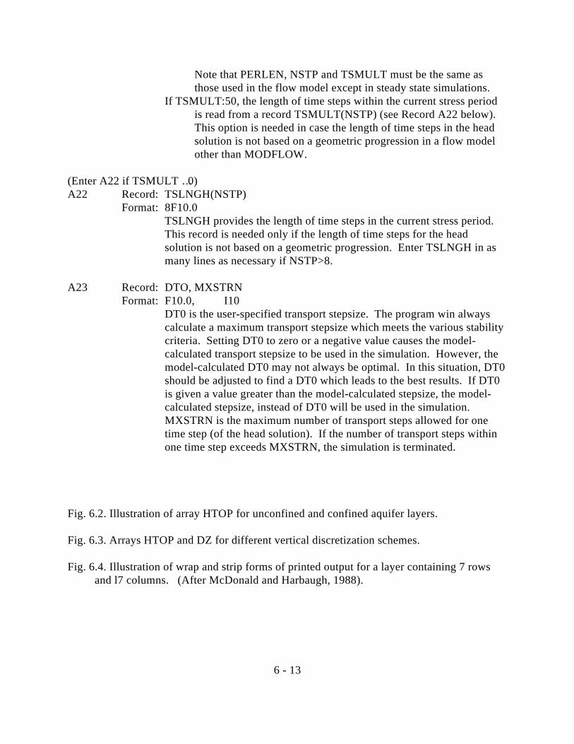
6 - 13
Note that PERLEN, NSTP and TSMULT must be the same asthose used in the flow model except in steady state simulations.
If TSMULT:50, the length of time steps within the current stress periodis read from a record TSMULT(NSTP) (see Record A22 below). This option is needed in case the length of time steps in the headsolution is not based on a geometric progression in a flow modelother than MODFLOW.
(Enter A22 if TSMULT …0)A22 Record: TSLNGH(NSTP)
Format: 8F10.0TSLNGH provides the length of time steps in the current stress period. This record is needed only if the length of time steps for the headsolution is not based on a geometric progression. Enter TSLNGH in asmany lines as necessary if NSTP>8.
A23 Record: DTO, MXSTRNFormat: F10.0, I10
DT0 is the user-specified transport stepsize. The program win alwayscalculate a maximum transport stepsize which meets the various stabilitycriteria. Setting DT0 to zero or a negative value causes the model-calculated transport stepsize to be used in the simulation. However, themodel-calculated DT0 may not always be optimal. In this situation, DT0should be adjusted to find a DT0 which leads to the best results. If DT0is given a value greater than the model-calculated stepsize, the model-calculated stepsize, instead of DT0 will be used in the simulation.MXSTRN is the maximum number of transport steps allowed for onetime step (of the head solution). If the number of transport steps withinone time step exceeds MXSTRN, the simulation is terminated.
Fig. 6.2. Illustration of array HTOP for unconfined and confined aquifer layers.
Fig. 6.3. Arrays HTOP and DZ for different vertical discretization schemes.
Fig. 6.4. Illustration of wrap and strip forms of printed output for a layer containing 7 rowsand l7 columns. (After McDonald and Harbaugh, 1988).
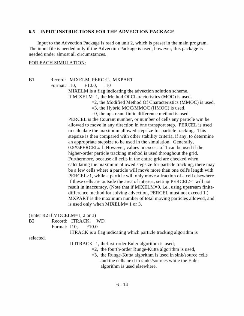
6 - 14
6.5 INPUT INSTRUCTIONS FOR THE ADVECTION PACKAGE
Input to the Advection Package is read on unit 2, which is preset in the main program. The input file is needed only if the Advection Package is used; however, this package isneeded under almost all circumstances.
FOR EACH SIMULATION:
B1 Record: MIXELM, PERCEL, MXPARTFormat: I10, F10.0, I10
MIXELM is a flag indicating the advection solution scheme.If MIXELM=1, the Method Of Characteristics (MOC) is used.
=2, the Modified Method Of Characteristics (MMOC) is used.=3, the Hybrid MOC/MMOC (HMOC) is used.=0, the upstream finite difference method is used.
PERCEL is the Courant number, or number of cells any particle win beallowed to move in any direction in one transport step. PERCEL is usedto calculate the maximum allowed stepsize for particle tracking. Thisstepsize is then compared with other stability criteria, if any, to determinean appropriate stepsize to be used in the simulation. Generally,0.5#5PERCEL# l. However, values in excess of 1 can be used if thehigher-order particle tracking method is used throughout the grid. Furthermore, because all cells in the entire grid are checked whencalculating the maximum allowed stepsize for particle tracking, there maybe a few cells where a particle will move more than one cell's length withPERCEL>1, while a particle will only move a fraction of a cell elsewhere. If these cells are outside the area of interest, setting PERCEL>1 will notresult in inaccuracy. (Note that if MIXELM=0, i.e., using upstream finite-difference method for solving advection, PERCEL must not exceed 1.)MXPART is the maximum number of total moving particles allowed, andis used only when MIXELM= 1 or 3.
(Enter B2 if MDCELM=1, 2 or 3)B2 Record: ITRACK, WD
Format: I10, F10.0ITRACK is a flag indicating which particle tracking algorithm is
selected.If ITRACK=1, thefirst-order Euler algorithm is used;
=2, the fourth-order Runge-Kutta algorithm is used,=3, the Runge-Kutta algorithm is used in sink/source cells
and the cells next to sinks/sources while the Euleralgorithm is used elsewhere.

6 - 15
WD is a concentration weighting factor between 0 and 1. The value of0.5 is normally a good choice. This number can be adjusted to achievebetter mass balance. Generally, it can be increased toward 1 asadvection becomes more dominant.
(Enter B3 ff MIXELM=1 or 3)B3 Record: DCEPS, NPLANE, NPL, NPH, NPMIN, NPMAX, SRMULT
Format: F10.0, I10, I10, I10, I10, I10, F10.0DCEPS is a small relative concentration gradient (DCCELL), such as 10-
, which is considered to be negligible.5
NPLANE is a flag indicating whether the random or fixed pattern isselected for initial placement of moving particles.If NPLANE=O, the the random pattern is selected for initial placement.
particles are distributed randomly by calling a random numbergenerator in both the horizontal and vertical directions (refer toFig. 4.9b). This option generally leads to smaller mass balancediscrepancy in nonuniform or diverging/converging flow fields.
If NPLANE>O, the fixed pattern is selected for initial placement. Thevalue of NPLANE serves as the number of vertical "planes" onwhich initial particles are placed within each cell block (refer toFig. 4.9a). This fixed pattern works well in relatively uniformflow fields. For two-dimensional simulations in plan view, setNPLANE=1. For cross sectional or three-dimensionalsimulations, NPLANE=2 is normally adequate. IncreaseNPLANE if more resolution in the vertical direction is desired.
NPL is number of initial particles per cell to be placed at cells whereDCCELL#DCEPS. Generally, NPL can be set to 0 since advection isinsignificant under the condition DCCELL#DCEPS. Setting NPL equalto NPH causes a uniform number of particles to be placed in every cellover the entire gdd (i.e., the uniform approach).
NPH is number of initial particles per cell to be placed at cells whereDCCELL>DCEPS. The selection of NPH depends on the nature of theflow field and also the computer memory limitation. Generally, use asmaller number in relatively uniform flow fields and a larger number inrelatively nonuniform flow fields. However, values exceeding 16 intwo-dimensional simulation or 32 in three-dimensional simulation arerarely necessary. If the random pattern is chosen, NPH particles arerandomly distributed within the cell block. If the fixed pattern is chosen,NPH is divided by NPLANE to yield the number of particles to beplaced per vertical plane, which is rounded to one of the values shown inFig. 6.5 NPMIN is the minimum number of moving particles allowed per

6 - 16
cell. If the number of particles in a cell at the end of a transport step isfewer than NPMIN, new particles are inserted into that cell to maintain asufficient number of particles. NPMIN can be set to 0 in relativelyuniform flow fields, and a number greater than zero indiverging/converging flow fields. Generally, 0# NPMIN# 4 is adequate.NPMAX is the maximum number of particles allowed per cell. If thenumber of particles in a cell exceeds NPMAX, particles are removedfrom that cell until NP is met. Generally, NPMAX can be set to a valueapproximately twice the value of NPH.SRMULT is a multiplier for the particle number at source cells(SRMULT$ l ). In most cases, SRMULT=1 is sufficient. However,better results may be obtained by increasing SRMULT.
(Enter B4 if MIXELM=2, or 3)B4 Record: INTERP, NLSINK, NPSINK
Format: 3110INTERP is a flag indicating the concentration interpolation method foruse in the MMOC solution scheme. Currently, only linear interpolationis implemented. Enter INTERP=L.NLSINK is a flag indicating whether the random or fixed pattern isselected for initial placement of particles to approximate sink cells in theMMOC scheme. The convention is the same as that for NPLANE.NPSINK is the number of particles used to approximate sink cells in theMMOC scheme. The convention for is the same as that for NPH.
(Enter B5 if MDCELM=3)B5 Record: DCHMOC
Format: F10.0DCHMOC is the critical relative concentration gradient for controllingthe selective use of either MOC or MMOC in the HMOC solutionscheme.The MOC solution is selected at cells where DCCELL>DCHMOC.The MMOC solution is selected at cells where DCCELL< DCHMOC.
Fig. 6.5. Distribution of initial particies using the fixed pattern. If the fixed pattern is chosen,the number of particles placed per cell (NPL and NPH) is divided by the numberof vertlcal "planes', or NPLANE, to yield the number of particles to be pieced oneach vertical plane, which is then rounded to one of the values shown here.

6 - 17
6.6 INPUT INSTRUCTIONS FOR THE DISPERSION PACKAGE
Input to the Dispersion Package is read on unit 3, which is preset in the main program. The input file is needed only if the Dispersion Package is used in the simulation.
FOR EACH SIMULATION:C1 Array: AL(NCOL,NROW) (One array for each layer).
Reader: RARRAYAL is the longitudinal dispersivity (% ) for each cell in the grid. (Unit: L).L
C2 Array: TRPT(NLAY)Reader: RARRAY
TRPT is the ratio of the horizontal transverse dispersivity (% ) to theTH
longitudinal dispersivity (% ) One value is specified for each layer.L
C3 Array: TRPV(NLAY)Reader: RARRAY
TRPV is the ratio of the vertical transverse dispersivity (% ) to theTV
longitudinal dispersivity (% ). One value is specified for each layer. SetL
TRPV equal to TRPT to use the standard isotropic dispersion model(equation 2.9 in Section 2.3.2). If TRPV is entered not equal to TRPT,the modified isotropic dispersion model is used (equation 2.10).
C4 Array: DMCOEF(NLAY)Reader: RARRAY
DMCOEF is the effective molecular diffusion coefficient. (Unit: L T ). 2 -1
Set DMCOEF=0 if the effect of molecular diffusion is consideredunimportant. One value is specified for each layer.
6.7 INPUT INSTRUCTIONS FOR SINK & SOURCE MIXING PACKAGE
Input to the Sink & Source Mixing Package is read on unit 4, which is preset in the mainprogram. The input file is needed if any sink or source option is used in the flow model,including the constant-head or general-head-dependent boundary conditions. Theclassification of the sink/source type used in MT3D is the same as that used by MODFLOW(McDonald and Harbaugh, 1988).
6 - 18
FOR EACH SIMULATION:
Dl Record: FWEL, FDRN, FRCH, FEVT, FRIV, FGHBFormat: 6L2
FWEL is a logical flag for the Well option;FDRN is a logical flag for the Drain option;FRCH is a logical flag for the Recharge option;FEVT is a logical flag for the Evapotranspiration option;FRIV is a logical flag for the River option; andFGHB is a logical flag for General-Head-Dependent Boundary option.If any of these options is used in the flow model, its respective flag mustbe set to T, otherwise, set to F.
D2 Record: MXSSFormat: I10
MXSS is the maximum number of all point sinks and sources simulatedin the flow model. Point sinks and sources include constant-head cells,wells, drains, rivers, and general-head-dependent boundary cells. Recharge and evapotranspiration are treated as areally distributed sinksand sources; thus, they should not be counted as point sinks and sources. MXSS should be set close to the actual number of total point sinks andsources in the flow model in order to minimize the computer memoryallocated to store sinks and sources.
FOR EACH STRESS PERIOD:
(Enter D3 if FRCH=T)D3 Record: INCRCH
Format: I10INCRCH is a flag indicating whether an array containing theconcentration of recharge fluxwill be read for the current stress period.If INCRCH>O, an array containing the concentration of recharge
flux will be read.<O, the concentration of recharge flux will be reused
from the last stress period. If INCRCH<O isentered for the first stress period, theconcentration of recharge flux is set to zero bydefault.
(Enter D4 if FRCH=T and INCRCH > 0)D4 Array: CRCH(NCOL,NROW)
Reader: RARRAY
6 - 19
CRCH is the concentration of recharge flux. If the recharge flux ispositive, the recharge acts as a source whose concentration can bespecifled as desired. If the recharge flux is negative, the recharge acts asa sink (or discharge) whose concentration is always set equal to theconcentration of the aquifer at the cell where discharge occurs. Note thatthe location and flow rate of recharge/discharge are obtained from theflow model directly through the unformatted head and flow file.
(Enter D5 if FEVT=T)D5 Record: INCEVT
Format: I10INCEVT is a flag indicating whether an array containing theconcentration of evapotranspiration flux will be read for the currentstress period. If INCEVT $ 0, and array containing the concentration of
evapotranspiration flux will be read.<0, the concentration of evapotranspiration flux will
be reused from the last stress period.
(Enter D6 if FEVT=T and INCEVT $ 0)D6 Array: CEVT(NCOL,NROW)
Reader: RARRAYCEVT is the concentration of evapotranspiration flux. Evapotranspiration is the only sink whose concentration can be specifiedexternally. Note that the concentration of a sink cannot be greater thanthat of the aquifer at the sink cell. Thus, if the sink concentration isspecified greater than that of the aquifer, it is automatically set equal tothe concentration of the aquifer. Note that the location and flow rate ofevapotranspiration are obtained from the flow model directly through theunfonmtted head and flow file.
D7 Record: NSSFormat: I10
NSS is the number of point sources whose concentrations need to bespecified. Unspecified point sources are assumed to have a zeroconcentration by default.(Note that the concentration of point sinks are always set equal to theconcentration of the aquifer).
(Enter D8 if NSS>O)D8 Record: KSS, ISS, JSS, CSS, ITYPE
Format: I10, I10, I10, F10.0,I10

6 - 20
KSS, ISS, JSS are the cell indices (layer, row, column) of the pointsource for which a concentration is to be specified. CSS is the specifiedconcentration. E is an integer number indicating the type of the pointsource as listed below. Enter one record for each point source ofspecified concentration. Note that the location and flow rate of pointsources/sinks are obtained from the flow model directly through theunformatted head and flow file.ITYPE =1, constant-head cell;
=2, well;=3, drain;=4, river;=5, general-head-dependent boundary cell.
6.8 INPUT INSTRUCTIONS FOR THE CHEMICAL REACTION PACKAGE
Input to the Chemical Reaction Package is read on unit 5, which is preset in the mainprogram. The input file is needed only if a sorption isotherm or a first-order rate reaction (decayor biodegradation) is simulated.
FOR EACH SIMULATION:E1 Record: ISOTHM, IREACT
Format: 2I10ISOTHM is a flag indicating whether, or if any, which sorption type issimulated.If ISOTHM =l, Linear isotherm is simulated.
=2, Freundlich isotherm is simulated.=3, Langmuir isotherm is simulated.=0, no sorption isotherm is simulated.
IREACT is a flag indicating whether the first-order rate reaction issimulated.
If IREACT =1, radioactive decay or biodegradation is simulated.=0, no first-order rate reaction is simulated
(Enter E2 if ISOTHM>0)E2 Array: RHOB(NLAY)
Reader: RARRAYRHOB is the bulk density of the porous medium in the aquifer. (Unit: ML-
). One value is specified for each layer.3
(Enter E3 if ISOTHM>O)E3 Array: SP1 (NLAY)
6 - 21
Reader: RARRAYSP1 is the first sorption constant. One value is specified each layer. The
use of SP 1 depends on the type of sorption selected (i.e.,ISOTHM).
For linear sorption, SP1 is the distribution coefficient (K ). (Unit: L M ).d3 -1
For Freundlich sorption, SP1 is the Freundlich sorption equilibriumconstant (K ). (Unit depends on the Freundlich exponent a).f
For Langmuir sorption, SP1 is the Langmuir sorption equilibrium constant(K ). (Unit: L M ).1
3 -l
(Enter E4 if ISOTHM>O)E4 Array: SP2(NLAY)
Reader: RARRAYSP2 is the second sorption constant. One value is specified for each layer.The use of SP2 depends on the type of sorption selected (i.e., ISOTHM).For linear sorption, SP2 is not used, but still must be entered.For Freundlich sorption, SP2 is the Freundlich exponent (a).For Langmuir sorption, SP2 is the total concentration of sorption sites
available ( ). (Unit: MM ).-1
(Enter E5 ff IREACT>0)E5 Array: RC1(NLAY)
Reader: RARRAYRC1 is the first-order rate constant for the dissolved phase. (Unit: T ). One-1
value is specified for each layer.
(Enter E6 if IREACT >0 )E6 Array: RC2(NLAY)
Reader: RARRAYRC2 is the first-order rate constant for the sorbed phase. (Unit: T ). One-l
value is specified for each layer. Generally, if the reaction is radioactivedecay, SP2 should be set equal to SP1. However, for certain types ofbiodegradation, SP2 may be different from SP1.
6.9 START OF A SIMULATION RUN
There are two ways to start a simulation run. The first method is simply to type the name ofthe executable file. The program will prompt the user for the names of various input and outputfiles. An example is given below, where "C:\>" is the command prompt and "MT3D" is the nameof the executable file of the MT3D program:
C: \>MT3D

6 - 22
M T 3 DA Modular Three-Dimensional Transport Model
For Simulation Advection, Dispersion and Chemical Reactionsof Contaminants in Groundwater Systems
Enter Name for Standard Output File: MT3D.OUTEnter Name for Basic Transport Input File: BTN.INPEnter Name for Advection Input File: ADV. INPEnter Name for Dispersion Input File: DSP.INPEnter Name for Sink & Source Input File: SSM.INPEnter Name for Chemical Reaction Input File: RCT.INPEnter Name for Unformatted Head & Flow File: MOD.FLOPrint out Heads and Flow Terms for Checking (Y/N)? N
STRESS PERIOD NO. 1TIME STEP NO. 1FROM TIME = 0.00000 TO 100.00Transport Step: 10 step size: 10.000 Tota1 Elapsed Time: 100.000Program Completed.
The second method is to create a response file which contains the names of input and outputfiles in the order required by the program. The content of such a response file (RUN.RL) forthe example shown above would be as follows:
MT3D.OUTBTN. INPADV. INPDSP.INPSSM. INPRCT. INPMOD.FLONThen, at the command prompt,
C:\> MT3D < RUN.FIL
6.10 CONTINUATION OF A PREVIOUS SIMULATION RUN
Sometimes it may be necessary to break a long simulation run into several shorter ones. For example, if the flow model has many stress periods and time steps, the unformatted headand flow file generated by the flow model can be quite large. If there is not enough diskspace, one has to break the simulation time into several intervals, with each interval having aseparate head and flow file. Then, one needs to run the transport model once for each interval

6 - 23
of the flow solution. The continuation of a previous simulation run in the MT3D transportmodel is imiiar to the continuation of a flow simulation in the MODFLOW flow model.
First, save the concentrations from the final step of the preceding run on the defaultunformatted file MT3D.UCN. Next, re-name the file and use it as the starting concentrationflle for the next run. (If there is more than one step of concentrations saved in the MT3D.UCNfile, extract the concentrations at the last step using a program called SAVELAST included inthe Postprocessing Program Disk.) The array reader which reads the starting concentrations(RARRAY) is capable of reading a model-generated unformatted concentration file with nomodification. Because mass budget terms are always set to zero at the start of a simulationrun, the printed budget on a simulation run represents only that single run. Therefore, if atotal budget for a series of continuation runs is desired, the totals from each run can be addedexternally. Similarly, the model program keeps track of simulation time only for singlesimulation runs; total simulation time for a series of continuation runs must be calculatedexternally by adding the simulation times of each run.
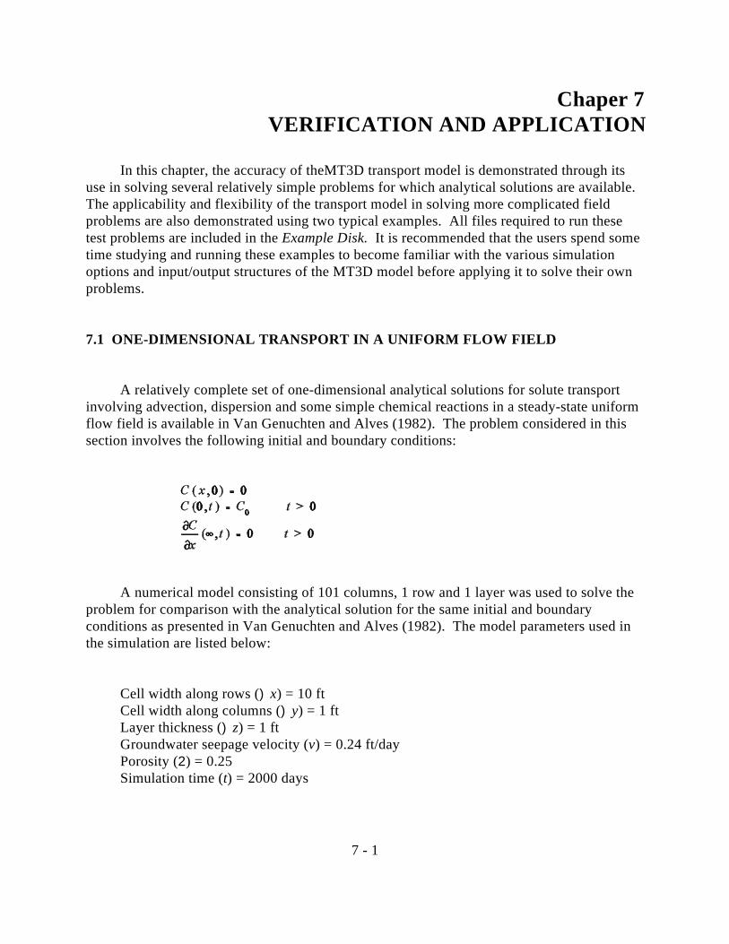
7 - 1
Chaper 7VERIFICATION AND APPLICATION
In this chapter, the accuracy of theMT3D transport model is demonstrated through itsuse in solving several relatively simple problems for which analytical solutions are available. The applicability and flexibility of the transport model in solving more complicated fieldproblems are also demonstrated using two typical examples. All files required to run thesetest problems are included in the Example Disk. It is recommended that the users spend sometime studying and running these examples to become familiar with the various simulationoptions and input/output structures of the MT3D model before applying it to solve their ownproblems.
7.1 ONE-DIMENSIONAL TRANSPORT IN A UNIFORM FLOW FIELD
A relatively complete set of one-dimensional analytical solutions for solute transportinvolving advection, dispersion and some simple chemical reactions in a steady-state uniformflow field is available in Van Genuchten and Alves (1982). The problem considered in thissection involves the following initial and boundary conditions:
A numerical model consisting of 101 columns, 1 row and 1 layer was used to solve theproblem for comparison with the analytical solution for the same initial and boundaryconditions as presented in Van Genuchten and Alves (1982). The model parameters used inthe simulation are listed below:
Cell width along rows ()x) = 10 ftCell width along columns ()y) = 1 ftLayer thickness ()z) = 1 ftGroundwater seepage velocity (v) = 0.24 ft/dayPorosity (2) = 0.25Simulation time (t) = 2000 days
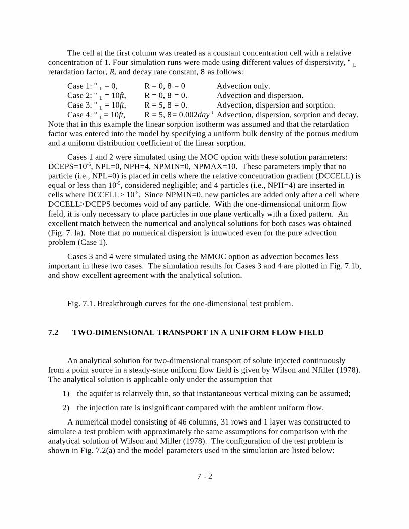
7 - 2
The cell at the first column was treated as a constant concentration cell with a relativeconcentration of 1. Four simulation runs were made using different values of dispersivity, "L
retardation factor, R, and decay rate constant, 8 as follows:
Case 1: " = 0, R = 0, 8 = 0 Advection only.L
Case 2: " = 10ft, R = 0, 8 = 0. Advection and dispersion.L
Case 3: " = 10ft, R = 5, 8 = 0. Advection, dispersion and sorption.L
Case 4: " = 10ft, R = 5, 8= 0.002day Advection, dispersion, sorption and decay. L -1
Note that in this example the linear sorption isotherm was assumed and that the retardationfactor was entered into the model by specifying a uniform bulk density of the porous mediumand a uniform distribution coefficient of the linear sorption.
Cases 1 and 2 were simulated using the MOC option with these solution parameters:DCEPS=10 , NPL=0, NPH=4, NPMIN=0, NPMAX=10. These parameters imply that no-5
particle (i.e., NPL=0) is placed in cells where the relative concentration gradient (DCCELL) isequal or less than 10 , considered negligible; and 4 particles (i.e., NPH=4) are inserted in-5
cells where DCCELL> 10 . Since NPMIN=0, new particles are added only after a cell where-5
DCCELL>DCEPS becomes void of any particle. With the one-dirnensional uniform flowfield, it is only necessary to place particles in one plane vertically with a fixed pattern. Anexcellent match between the numerical and analytical solutions for both cases was obtained(Fig. 7. la). Note that no numerical dispersion is inuwuced even for the pure advectionproblem (Case 1).
Cases 3 and 4 were simulated using the MMOC option as advection becomes lessimportant in these two cases. The simulation results for Cases 3 and 4 are plotted in Fig. 7.1b,and show excellent agreement with the analytical solution.
Fig. 7.1. Breakthrough curves for the one-dimensional test problem.
7.2 TWO-DIMENSIONAL TRANSPORT IN A UNIFORM FLOW FIELD
An analytical solution for two-dimensional transport of solute injected continuouslyfrom a point source in a steady-state uniform flow field is given by Wilson and Nfiller (1978). The analytical solution is applicable only under the assumption that
1) the aquifer is relatively thin, so that instantaneous vertical mixing can be assumed;
2) the injection rate is insignificant compared with the ambient uniform flow.
A numerical model consisting of 46 columns, 31 rows and 1 layer was constructed tosimulate a test problem with approximately the same assumptions for comparison with theanalytical solution of Wilson and Miller (1978). The configuration of the test problem isshown in Fig. 7.2(a) and the model parameters used in the simulation are listed below:

7 - 3
Cell width along rows ()x) = 10 mCell width along columns ()y) = 10 mLayer thickness ()z) = 10 mGroundwater seepage velocity (v) = 1/3 m/dayPorosity (2) = 0.3Longitudinal dispersivity = 10 mRatio of transverse to longitudinal dispersivity = 0.3Volumetric injection rate = 1 m /day3
Concentration of the injected water = 1000 ppmSimulation time (t) = 365 days
The hybrid MOC/MMOC, or HMOC option was used in the simulation, withDCHMOC set to 10 and the rest of the solution parameters as follows:-3
(for the MOC scheme):
DCEPS=10 , NPLANE=1, NPL=0, NPH=9, NPMIN=0, NPMAX=16-5
(for the MMOC scheme):
INTERP=l NLSINK=1, NPSINK=9
Thus, in the solution process, the MOC scheme was automatically selected in cellswhere DCCELL>10 ; and the MMOC scheme was automatically selected in cells where-3
DCCELL # 10 . When the MOC scheme was used, 9 particles were placed in cells with a-3
fixed pattern on one vertical plane (NPLANE=l) where DCCELL is greater than the specifiednegligible limit. When the MMOC scheme was used, 1 fictitious particle was placed at thenodal point for backward tracking except at a sink cell where 9 particles were placed (i.e.,NPSINK=9) on one (1) vertical plane within the sink cell block (i.e., NLSINK=l). The optionselected for particle tracking is ITRACK=3. In other words, the fourth-order Runge-Kuttamethod is used in the vicinity of the point source whereas the first Euler method is usedelsewhere.
The contour map of the concentration field at the end of the 365-day simulation periodobtained for this test problem is shown in Fig. 7.2. The numerical solution agrees well withthe analytical solution.
The HMOC option offered some advantage over either MOC or MMOC option alone inthis example. The MMOC option alone can lead to some numerical dispersion with the Pecletnumber (Pe) equal to 1 along the x-direction. The MOC option alone requires about 7000particles at the end of the 1-year simulation period. One the other hand, the HMOC optionvirtually eliminates the numerical dispersion while using approximately half the total numberof moving particles required by the MOC option alone. The DCHMOC criterion is a

7 - 4
empirical value, and requires some trial and error before an optimal number may bedetermined. However, as found in this and subsequent test examples, values between 0.01and 0.001 are normally adequate.
Fig. 7.2. Comparison of the numerical and analytical solutions for two-dimensional froma point source in a uniform flow field.
7.3 TWO-DIMENSIONAL TRANSPORT IN A RADIAL FLOW FIELD
The problem considered in this section concerns the two-dimensional transport of soluteinjected from a fully penetrating well. The assumptions for this problem are:
1) the injection rate of the well is constant;
2) the ambient groundwater velocity is negligible relative to the velocity created by theinjection;
3) the aquifer is homogeneous, isotropic, and infinite in areal extent; and
4) the flow field is steady-state.
The initial and boundary conditions for this problem are
where r is the well radius. An approximate analytical solution for this problem is given byw
Moench and Ogata (1981) and available in a computer program (LTIRD) provided byJavandel et. al. (1984).
A numerical model consisting of 31 columns, 31 rows and 1 layer was used to solve thisproblem for comparison with the analytical solution of Moench and Ogata (1981). The modelparameters used in the simulation are listed below:
Cell width along rows ()x) = 10 ftCell width along columns ()y) = 10 ftLayer thickness ()z) = 1 ft
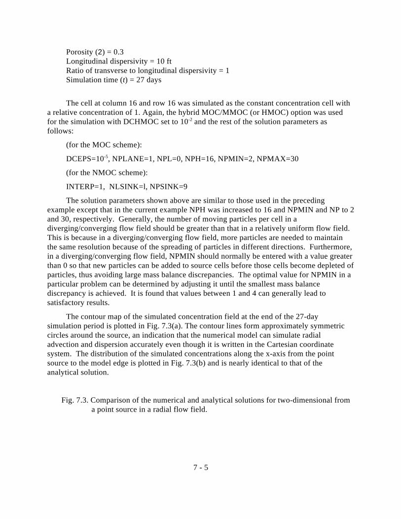
7 - 5
Porosity (2) = 0.3Longitudinal dispersivity = 10 ftRatio of transverse to longitudinal dispersivity = 1Simulation time (t) = 27 days
The cell at column 16 and row 16 was simulated as the constant concentration cell witha relative concentration of 1. Again, the hybrid MOC/MMOC (or HMOC) option was usedfor the simulation with DCHMOC set to 10 and the rest of the solution parameters as-2
follows:
(for the MOC scheme):
DCEPS=10 , NPLANE=1, NPL=0, NPH=16, NPMIN=2, NPMAX=30 -5
(for the NMOC scheme):
INTERP=1, NLSINK=l, NPSINK=9
The solution parameters shown above are similar to those used in the precedingexample except that in the current example NPH was increased to 16 and NPMIN and NP to 2and 30, respectively. Generally, the number of moving particles per cell in adiverging/converging flow field should be greater than that in a relatively uniform flow field. This is because in a diverging/converging flow field, more particles are needed to maintainthe same resolution because of the spreading of particles in different directions. Furthermore,in a diverging/converging flow field, NPMIN should normally be entered with a value greaterthan 0 so that new particles can be added to source cells before those cells become depleted ofparticles, thus avoiding large mass balance discrepancies. The optimal value for NPMIN in aparticular problem can be determined by adjusting it until the smallest mass balancediscrepancy is achieved. It is found that values between 1 and 4 can generally lead tosatisfactory results.
The contour map of the simulated concentration field at the end of the 27-daysimulation period is plotted in Fig. 7.3(a). The contour lines form approximately symmetriccircles around the source, an indication that the numerical model can simulate radialadvection and dispersion accurately even though it is written in the Cartesian coordinatesystem. The distribution of the simulated concentrations along the x-axis from the pointsource to the model edge is plotted in Fig. 7.3(b) and is nearly identical to that of theanalytical solution.
Fig. 7.3. Comparison of the numerical and analytical solutions for two-dimensional froma point source in a radial flow field.

7 - 6
7.4 CONCENTRATION AT AN INJECTION/EXTRACTION WELL
Injection/extraction wells are commonly used in practice to contain and clean upcontaminants in groundwater. Therefore, in many practical transport simulations involvingevaluation of the effectiveness of remedial alternatives, it is important for the transport modelto have the ability to approximate closely the concentrations at injection/extraction wells.
A problem involving an injection/pumping cycle for a fully penetrating well in aconfined aquifer was used to test this capability of the MT3D transport model. Water of aconstant concentration (C ) was injected into the well. After a certain period of time (t ), the0 1
flow was reversed, and the contaminated water was pumped out. Assuming that the flow fieldreaches steady state instantaneously after the injection and pumping cycles start, anapproximate analytical solution for this problem is given by Gelhar and Collins (1971).
A numerical model consisting of 31 columns, 31 rows and 1 layer was used to simulatethe concentration change at the injection/extraction well for comparison with the approximateanalytical solution of Gelhar and Collins (1971). The model parameters used in thesimulation were the same as those used by El-Kadi (1988) to test the U.S. Geological Surveytwo-dimensional solute transport model (Konikow and Bredehoeft, 1978) as listed below:
Cell width along rows ()x) = 900 ftCell width along columns ()y) = 900 ftLayer thickness ()z)= 20 ftHydraulic conductivity of the aquifer = 0.005 ft/sPorosity (2) = 0.3Longitudinal dispersivity = 100 ftRatio of transverse to longitudinal dispersivity =1Volumetric injection/extraction rate = 1 ft /s3
Relative concentration of the injected water = 100 percentLength of the injection period = 2.5 yearsLength of the extraction period = 7.5 years
The MOC option was used in the simulation as the transport process is largelydominated by advection, with cell Peclet numbers in the vicinity of 10. The solutionparameters for the MOC scheme are NPL=16, NPH=16, NPMIN=4 and NPMAX=30. Because NPL is set equal to NPH, a uniform distribution of 16 particles per cell wasinitialized over the entire grid. Initial particles were placed randon-fly within each cell block. The selection of the random pattern over the fixed pattern leads to a smaller mass balancediscrepancy due to the strongly diverging/converging nature of the flow field. The fourth-order Runge-Kutta particle tracking algorithm was selected to increase the accuracy of thesolution.
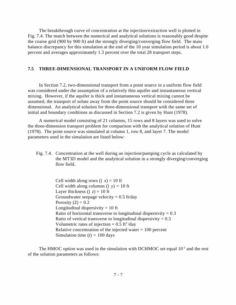
7 - 7
The breakthrough curve of concentration at the injection/extraction well is plotted inFig. 7.4. The match between the numerical and analytical solutions is reasonably good despitethe coarse grid (900 by 900 ft) and the strongly diverging/converging flow field. The massbalance discrepancy for this simulation at the end of the 10 year simulation period is about 1.0percent and averages approximately 1.3 percent over the total 28 transport steps.
7.5 THREE-DIMENSIONAL TRANSPORT IN A UNIFORM FLOW FIELD
In Section 7.2, two-dimensional transport from a point source in a uniform flow fieldwas considered under the assumption of a relatively thin aquifer and instantaneous verticalmixing. However, if the aquifer is thick and instantaneous vertical mixing cannot beassumed, the transport of solute away from the point source should be considered threedimensional. An analytical solution for three-dimensional transport with the same set ofinitial and boundary conditions as discussed in Section 7.2 is given by Hunt (1978).
A numerical model consisting of 21 columns, 15 rows and 8 layers was used to solvethe three-dimension transport problem for comparison with the analytical solution of Hunt(1978). The point source was simulated at column 1, row 8, and layer 7. The modelparameters used in the simulation are listed below:
Fig. 7.4. Concentration at the well during an injection/pumping cycle as calculated bythe MT3D model and the analytical solution in a strongly diverging/convergingflow field.
Cell width along rows ()x) = 10 ftCell width along columns ()y) = 10 ftLayer thickness ()z) = 10 ftGroundwater seepage velocity = 0.5 ft/dayPorosity (2) = 0.2Longitudinal dispersivity = 10 ftRatio of horizontal transverse to longitudinal dispersivity = 0.3Ratio of vertical transverse to longitudinal dispersivity = 0.3Volumetric rates of injection = 0.5 ft /day3
Relative concentration of the injected water = 100 percentSimulation time (t) = 100 days
The HMOC option was used in the simulation with DCHMOC set equal 10 and the rest-2
of the solution parameters as follows:
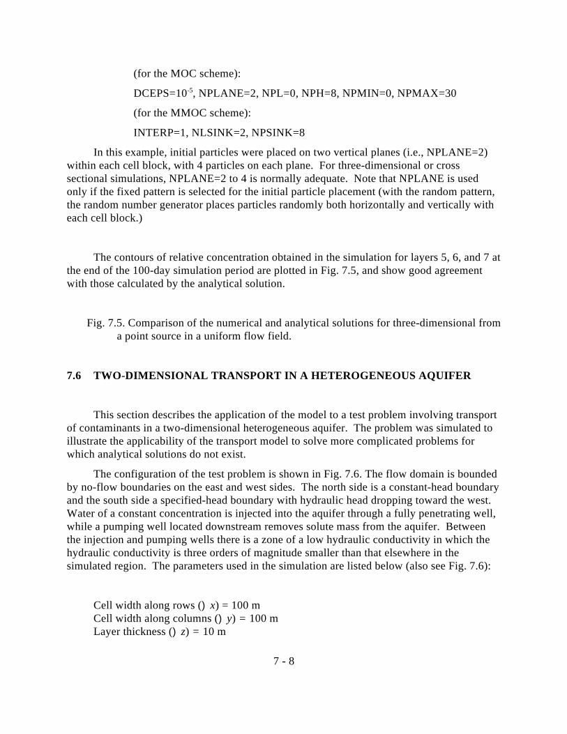
7 - 8
(for the MOC scheme):
DCEPS=10 , NPLANE=2, NPL=0, NPH=8, NPMIN=0, NPMAX=30 -5
(for the MMOC scheme):
INTERP=1, NLSINK=2, NPSINK=8
In this example, initial particles were placed on two vertical planes (i.e., NPLANE=2)within each cell block, with 4 particles on each plane. For three-dimensional or crosssectional simulations, NPLANE=2 to 4 is normally adequate. Note that NPLANE is usedonly if the fixed pattern is selected for the initial particle placement (with the random pattern,the random number generator places particles randomly both horizontally and vertically witheach cell block.)
The contours of relative concentration obtained in the simulation for layers 5, 6, and 7 atthe end of the 100-day simulation period are plotted in Fig. 7.5, and show good agreementwith those calculated by the analytical solution.
Fig. 7.5. Comparison of the numerical and analytical solutions for three-dimensional froma point source in a uniform flow field.
7.6 TWO-DIMENSIONAL TRANSPORT IN A HETEROGENEOUS AQUIFER
This section describes the application of the model to a test problem involving transportof contaminants in a two-dimensional heterogeneous aquifer. The problem was simulated toillustrate the applicability of the transport model to solve more complicated problems forwhich analytical solutions do not exist.
The configuration of the test problem is shown in Fig. 7.6. The flow domain is boundedby no-flow boundaries on the east and west sides. The north side is a constant-head boundaryand the south side a specified-head boundary with hydraulic head dropping toward the west. Water of a constant concentration is injected into the aquifer through a fully penetrating well,while a pumping well located downstream removes solute mass from the aquifer. Betweenthe injection and pumping wells there is a zone of a low hydraulic conductivity in which thehydraulic conductivity is three orders of magnitude smaller than that elsewhere in thesimulated region. The parameters used in the simulation are listed below (also see Fig. 7.6):
Cell width along rows ()x) = 100 mCell width along columns ()y) = 100 mLayer thickness ()z) = 10 m
7 - 9
Porosity (2) = 0.3Longitudinal dispersive = 20 ftRatio of horizontal transverse to longitudinal dispersive = 0.2Simulation time (t) = 1 year
The flow and transport models consist of 16 columns, 20 rows, and 1 layer. Theboundary conditions for the transport model are no-mass flux boundaries on the east, west,and north borders of the model. The south border was treated as a line of point sinks takingmass out of the aquifer.
Fig. 7.6. Configuration of the heterogeneous aquifer simulated in the test problem.
The HMOC option was used in the transport simulation with DCHMOC set equal to2xl0 and the rest of the solution parameters as follows:-3
(for the MOC scheme):
DCEPS=10 , NPLANE=0, NPL=0, NPH=16, NPMIN=2, NPMAX=30 -5
(for the MMOC scheme):
INT'ERP=1, NLSINK=0, NPSINK=16
Initial particles were distributed using the random pattern (NPLANE=0). The fourth-order Runge-Kutta algorithm (i.e., ITRACK=2) was selected to move all particles to ensurethe accuracy of the particle tracking calculations in the heterogeneous aquifer. In the previousexamples, the number of cells a particle was allowed to move in any direction (i.e., PERCEL)was always set equal to a value between 0.5 and 1.0. In other words, no particles wereallowed to move more than one cell's length in any direction. However, in the currentexample, PERCEL=1.5 was found to give better mass balance results than PERCEL=1.0, withall other parameters held the same.
T'he simulated concentration field at the end of 1-year simulation period is plotted inFig. 7.7. The mass balance discrepancy for this simulation is shown in Fig. 7.8. While thediscrepancy tends to be relatively large at early times, it decreases to near zero as simulationcontinues. The average for the full simulation (28 transport steps) is less than 0.3%,indicating that the mass injected into the aquifer is largely conserved.
It is interesting to compare Fig. 7.7 with Fig. 7.9 which shows the concentration fieldfor this problem as simulated by the pure finite difference method. While the general patternsof these two simulated plumes are quite similar, it is clear that the pure finite differencesolution introduces a certain amount of numerical dispersion, which causes artificial smearingof the plume.

7 - 10
Fig. 7.7. Distribution of solute concentrations as solved by the hybrid MOC/MMOC (HMOC)solution.
Fig. 7.8. Plot of the mass balance discrepancy error at each rt step for the test probleminvolving a heterogeneous aquifer.
Fig. 7.9. Distribution of solute concentrations as solved by the finite difference solution forcomparison with those solved by the hybrid MOC/MMOC (HMOC)solution (Fig.7.7).
7.7 A THREE-DIMENSIONAL FIELD APPLICATION
This section describes the application of the MT3D transport model to an actual fieldproblem involving evaluation of the effectiveness of proposed groundwater remediationschemes; the discussion is intended to demonstrate the performance of the model in arepresentation of real world problems. The geologic setting of the site is illustrated in Fig. 7.10. The aquifer is unconfined and consists mostly of medium-grained sand exhibiting twodistinctive hydraulic conductivities, about 60 ft/day in the shallow zone and approximately600 ft/day in the deeper zone. The recharge rate estimated for the site is 5 inches per year. The porosity value is approximately 30 percent. Several organic compounds have beendetected in groundwater beneath the site. Among them is 1,2-dichloroethane (1,2-DCA),which is found over an area of more than 2200 feet by 1300 feet, with the maximumconcentration exceeding 200 ppb.
A numerical model was developed for this site to investigate the effectiveness andperformance of various remedial scenarios designed to clean up the aquifer. The modelconsisted of four layers in the vertical direction as shown in Fig. 7.10. In plan view, 61 rowsand 40 columns were used (see Fig. 7.11). The boundaries were set sufficiently far awayfrom the site to minimize their effect on flow and transport in the immediate vicinity of thesite. Most of the cers were concentrated in the central part of the mesh, denoted ABCD inFig. 7.11, in the area of the contaminant plume. The flow field was simulated using theMODFLOW flow model assuming the steady-state condition.
The present distribution of 1,2-dichoroethane (time=0) is shown in Fig. 7.12a. One ofthe scenarios for cleanup is to use 8 extraction wells (shown in the figure as squares labelledfrom Wl to W8) to pump contaminated groundwater out of the aquifer for treatment. Thelongitudinal dispersivity used for the modeling is 10 feet, with horizontal and verticaltransverse dispersivities of 2 feet. A uniform retardation factor equal to 2 was calculated from
7 - 11
the uniform bulk density and distribution coefficient selected. The proposed total extractionrate for the eight wells was about 700 gpm, all from layer 3.
The IMOC option was used in the transport simulation with DCHMOC set to 10 and-2
the rest of the solution parameters as follows:
(for the MOC scheme):
DCEPS=10 , NPLANE=0, NPL=0, NPH=10, NPMIN=2, NP =30-5
(for the MMOC scheme):
INTERP=1, NLSINK=0, NPSINK=10
Initial particles were distributed using the random pattern (NPLANE=0). The randompattern was found to be superior to the fixed pattern in this application due to the nature of theflow field. The mixed first-order Euler and fourth-order Runge-Kutta algorithm (i.e.,ITRACK=3) was selected for particle tracking in the heterogeneous aquifer. The Courant
number (i.e., PERCEL) was set equal to 1.0. The concentration weighting factor (i.e., WD)was entered as 0.5.
The concentration distributions in layer 3 within area ABCD after 500, 750 and 1000days from the time when pumping starts, as predicted by the MT3D transport model, areshown in Figs. 7.12b, 7.12c and 7.12d, respectively. The concentration breakthrough curvesat pumping wells Wl, W4 and W6, which are located in the the northern end, middle point,and southern end of the plume, respectively, are plotted in Fig. 7.13. The mass balancediscrepancy at the end of the 1000-day simulation period was about 2.7 percent, and averaged3.8 percent over the 128 transport steps in the entire simulation.
Fig. 7.10. Setting and vertical discretization in the field example.
Fig. 7.11. Plan view of the finite difference mesh for the field example.
Fig. 7.12. Present distribution of the disolved l,2-DCA and the model-predicted concentrationchanges at selected times after pumping starts
Fig. 7.13. Concentration breakthrough curves at pumping wells W1, W4 and located at thenorthern end, middle area and southern end of the plume, respectively. (Concentrations are shown in the plot every five steps.)

8-1
References
Anderson, M.P. 1979. Using models to simulate the movement of contaminants throughgroundwater flow systems. CRC Critical Rev. Environ. Control., 9(2), p. 97-156.
Anderson, M.P. 1984. Movement of contaminants in groundwater: groundwater transport--advection and dispersion. Groundwater Contamination. National Academy Press,Washington, D.C. p. 37-45.
Bear, J. 1972. Dynamics of Fluids in Porous Media. Elsvier Scientific Publishing Company. 764 pp.
Bear J. 1979. Hydraulics of Groundwater. McGraw-Hill, New York. 210 pp.
Beljin, S.B. 1990. SOLUTE--a program package of analytical models for solute transport ingroundwater, version 2.0 users's manual. International Ground Water ModelingCenter. 93 pp.
Burnett, R.D. and E.O. Frind. 1987. An alternating direction Galerkin technique for simula-tion of groundwater contaminant transport in three dimensions, 2, Dimensionalityeffects. Water Resour. Res., 23(4), p. 695-705.
Cheng, R.T., V. Casulli and S.N. Milford. 1984. Eulerian-Lagrangian solution of theconvection-dispersion equation in natural coordinates. Water Resour. Res., 20(7), p.944-952.
El-Kadi, A.I. 1988. Applying the USGS mass-transport model (MOC) to remedial actions byrecovery wells. Ground Water, 26(3), p. 281-288.
Farmer, C.L. 1987. Moving particle techniques, In Advances in transport phenomena inporous media. J. Bear and M.Y. Corapcioglu (eds.), NATO ASI Series #128, Nijhoff,Boston. p. 952-1004.
Garder, A.O., Jr., D.W. Peaceman and A.L. Pozzi, Jr. 1964. Numerical calculation of multidi-mensional miscible displacement by the method of characteristics. Soc. Pet. Eng. J.,6(2), p. 175-182.
Golden Software, Inc. 1989. SURFER® Version 4.0 Reference Manual. Golden, CO.
Gelhar, L.W. and M.A. Collins. 1971. General analysis of longitudinal dispersion in nonuni-form flow. Water Resour. Res., 7(6), p. 1511-1521.

8-2
Goode, D.J. 1990. Particle velocity interpolation in block-centered finite difference ground-water flow models. Water Resour. Res., 26(5), p. 925-940.
Goode, D.J. and L.F. Konikow. 1989. Modification of a method-of-characteristics solutetransport model to incorporate decay and equilibrium-controlled sorption and ionexchanges. U.S. Geological Survey Water-Resources Investigations Report 89-4030. 65 pp.
Grove, D.B. and K.G. Stollenwerk. 1984. Computer model of one-dimensional equilibrium-controlled sorption processes. U.S. Geological Survey Water-Resources InvestigationsReport 84-4059. 58 pp.
Healy, R.W. and T.F. Russell. 1989. Efficient implementation of the modified method ofcharacteristics in finite-difference models of solute transport. In Proceedings of 4th Int.Conf. on the use of models to analyze and find working solutions to groundwaterproblems. NWWA.
Hunt, B. 1983. Mathematical Analysis of Groundwater Resources. Butterworths, Cambridge.
Javandel. I., C. Doughty and C.F. Tsang. 1984. Groundwater Transport: Handbook ofMathematical Models. American Geophysical Union Water Resources Monogram 10.228 pp.
Konikow, L.F. and J.D. Bredehoeft. 1978. Computer model of two-dimensional solutetransport and dispersion in ground water. U.S. Geol. Surv. Water Resour. Invest. Book7, Chapter C2, 90 pp.
McDonald, J.M. and A.W. Harbaugh. 1988. A modular three-dimensional finite-differenceflow model. Techniques of Water Resources Investigations of the U.S. GeologicalSurvey, Book 6. 586 pp.
Moench, A.F. and A. Ogata. 1981. A numerical inversion of the Laplace transform solution toradial dispersion in a porous medium. Water Resour. Res., 17(1), p. 250-253.
Neuman, S.P. 1981. A Eulerian-Lagrangian numerical scheme for the dispersion-conversionequation using conjugate space-time grids. J. of Computational Physics, v. 41, p. 270-294.
Neuman, S.P. 1984. Adaptive Eulerian-Lagrangian finite element method for advection-dispersion. Int. J. Numerical Methods in Engineering, v. 20, p. 321-337.
Peaceman, D.W. 1977. Fundamentals of Numerical Reservoir Simulation. Elsvier ScientificPublishing Company. 74 pp.

8-3
Pollock, D.W. 1988. Semianalytical computation of path lines for finite-difference models.Ground Water, 26(6), p. 743-750.
Press, W.H., B.P. Flannery, S.A. Teukolsky and W.T. 1986. Numerical Recipes. UniversityCambridge Press. 818 pp.
Russell, T.F. and M.F. Wheeler. 1983. Finite element and finite difference methods forcontinuous flow in porous media. SIAM The Mathematics of Reservoir Simulation.R.E. Ewing (ed.), Chapter II., p. 35-106.
Van Genuchten, M.Th. and W.J. Alves. 1982. Analytical solutions of the one-dimensionalconvective-dispersive solute transport equation. U.S. Department of AgricultureTechnical Bulletin No. 1661, 151 pp.
Wilson, J.L. and P.J. Miller. 1978. Two-dimensional plume in uniform ground-water flow. J. Hyd. Div., ASCE, v.4, p. 503-514.
Yeh, G.T. 1990. A Lagrangian-Eulerian method with zoomable hidden fine-mesh approach tosolving advection-dispersion equations. Water Resour. Res., 26(6), p. 1133-1144.
Zheng, C. 1988. New solution and model for evaluation of groundwater pollution control.Ph.D. Dissertation, Univ. of Wisc.-Madison, 149 pp.
Zheng, C. 1989. PATH3D--a ground-water path and travel-time simulator, version 2.0 user'smanual. S.S. Papadopulos & Associates, Inc. 50 pp.

Appendix A
SPACE REQUIREMENTS

A - 2
Appendix ASPACE REQUIREMENTS
The elements of the X and IX arrays required by each package for a given problem are alwaysprinted by the model program every time it is run. They can also be calculated according tothe formulas given below. Variables used in the formulas are defined as follows:
NCOL = the total number of columns;NROW= the total nuumber of rows;NLAY = the total umber of layers;NODES= NCOL*NROW*NLAY, the total number of cells in the model;MXSS = the number of all point sinks and sources present in the flow
model, including constant-head and general-head-dependentboundary cells, but excluding recharge and evapotranspirationcells;
MXPART= the maximum number of moving particles allowed;ND = the number of dimensions in the given problem (ND=l for a one-
dimensional problem; 2 for a two-dimensional problem and 3 for a three-dimensional problem).
A. BASIC TRANSPORT PACKAGE (BTN)I. X Array
(ND+9)*NODES+2*NROW+2*NCOLII. IX Array
NODES+NLAYB. ADVECTION PACKAGE (ADV)
I. X Array(ND+l)*MXPART
II. IX ArrayNODES
C. DISPERSION PACKAGE (DSP)I. X Array
(ND +1)*NODES+3*NLAY2
II. DC ArrayNone
D. SINK & SOURCE MIXING PACKAGE (SSM)I. X Array
6*MXSSIf recharge is simulated, add 2*NROW*NCOLIf evapotranspiration is simulated, add 2*NROW*NCOL
II. IX ArrayIf recharge is simulated and NLAY>1, NROW*NCOLIf evapotranspiration is simulated and NLAY>1, add NROW*NCOL

A - 3
E. CHEMICAL REACTION PACKAGE (RCT)I. X Array
If sorption is simulated, 4*NLAYIf first-order rate reaction is simulated, add 2*NLAY
II. IX Array None
Appendix B
LINKING MT3D WITH A FLOW MODEL

B - 2
Appendix BLINKING MT3D WITH A FLOW MODEL
The Flow Model Interface Package of MT3D reads the hydraulic heads, fluxes across cellinterfaces in the row, column and layer directions, and locations and flow rates of the varioussources and sinks from an unformatted file saved by the flow model used in conjunction withthe MT3D transport model. If the U.S. Geological Survey modular flow model(MODFLOW) is used for the flow simulation, a package named LKMT, which is included inthe Flow Model Disk, can be linked to the MODFLOW program to save the followinginformation as explained in Section 6.2. If a flow model other than MODFLOW is used in theflow simulation, the flow model can be modified to save the heads and flow terms asinstructed below.
FOR EACH TIME STEP OF THE HEAD SOLUTION:
Fl. Record: KPER, KSTP, NCOL, NROW, NLAY, LABELF2. Record: H(NCOL,NROW,NLAY)
KPER--the stress period number at which the head and flow terms are saved KSTP--the time step number at which the head and flow terms are savedNCOL, NROW, NLAY--number of columns, rows and layers H--hyaulic heads. Heads at inactive cells must be set equal to l.E30.LABEL--'HEAD', identifying character label for heads
(If NCOL=l, skip F3 and F4)F3. Record: KPER, KSTP, NCOL, NROW, NLAY, LABELF4. Record: QX(NCOL,NROW,NLAY)
QX--volumetric fluxes between cells at cell interfaces along rows (or the x-axis).Positive in the direction of increasing J index.LABEL='QXX', identifying character label for QX
(If NROW= 1, skip F5 and F6)F5. Record: KPER, KSTP, NCOL, NROW, NLAY, LABELF6. Record: QY(NCOL,NROW,NLAY)
QY--volumetric fluxes between cells at cell interfaces along columns(or the y-axis). Positive in the direction of increasing I index.
LABEL='QYY', identifying character label for QYY (If NLAY=1, skip F7 and F8)F7. Record: KPER, KSTP, NCOL, NROW, NLAY, LABELF8. Record: QZ(NCOL,NROW,NLAY)
QZ--volumetric fluxes between cells at cell interfaces along layers (or the z-axis).Positive in the direction of increasing K index.LABEL='QZZ', identifying character label for QZ
F9. Record: KPER, KSTP, NCOL, NROW, NLAY, LABEL, NCNH NCNH--number of constant-head cells
B - 3
LABEL='CNH', identifying character label for constant head (If NCHN>0, there must be NCNH records of F10)F10. Record: KCNH,ICNH,JCNH,QCNH
KCNH,ICNH,JCNH-cell indices of each constant-head cellQCNH--volumetric net flow rate out of or into the constant-head cell, including
exchange between constant-heads (this is different from the net flowrate calculated at a constant-head cell in MODFLOW). Positive if flowis out of the constant head cell, negative otherwise.
(If wells are not present in the flow model, skip F11 and F12)F11. Record: KPER, KSTP, NCOL, NROW, NLAY, LABEL, NWEL
NWEL--number of wellsLABEL='WEL', identifying character label for well
(If NWERL>0, there must be records of F12)F12. Record: KWEL,IWEL, JWEL,QWEL
KWEL,IWEL,JWEL--cell indices of each wellQWEL--volumetric flow rate of the well. Positive if into the cell, negativeotherwise. (The same convention is followed by the remaining sink/source terms).
(If drains are not present in the flow model, skip F13 and F14)F13. Record: KPER, KSTP, NCOL, NROW, NLAY, LABEL,NDRN
NDRN--number of drainsLABEL='DRN', identifying character label for drain
(If NDRN>0, there must be NDRN records of F14)F14. Record: KDRN,IDRN,JDRN,QDRN KDRN,IDRN,JDRN--cell indices of each drain
QDRN--volumetric flow rate of the drain(If recharge is not present in the flow model, skip F15, F16 and F17)F15. Record: KPER, KSTP, NCOL, NROW, NLAY, LABEL
LABEL--'RCH', identifying character label for recharge(If NLAY= 1, skip F16)F16. Record: IRCH(NCOL,NROW)
IRCH--layer indices of the recharge fluxF17. Record: RECH(NCOL,NROW)
RECH--volumetric rate of recharge(If evapotranspiration is not present in the flow model, skip F18, F19, and F20)F18. Record: KPER,KSTP,NCOL,NROW,NLAY,LABEL
LABEL--'EVT', identifying character label for evapotranspiration(If NLAY=1, skip F19)F19. Record: IEVT(NCOL,NROW)
IEVT--layer indices of the evapotranspiration fluxF20. Record: EVTR(NCOL,NROW) EVTR--volumetric rate of evapotranspiration(If rivers are not present in the flow model, skip F21 and F22)F21. Record: KPER, KSTP, NCOL, NROW, NLAY, LABEL,NRIV

B - 4
NRIV--number of riversLABEL='RIV', identifying character label for river
(If NRIV>0, there must be NRIV records of F22)F22. Record: KRIV,IRIV,JRIV,QRIV
KRIV,IRIV,JRIVN--cell indices of each riverQRIV--volumetric flow rates of the river reaches
(If general-head-dependent boundaries not present in the flow model skip F23 and F24)F23. Record: KPER, KSTP, NCOL, NROW, NLAY, LABEL,NGHB
(If NGHB>0, there must be NGHB records of F24)F24. Record: KGHB,IGHB,JGHB,QGHBKGHB,IGHB,JGHB--cell indices of each general-head-dependent boundary cell QGHB--volumetric flow rates of the general-head-dependent boundary cells
Appendix CSAMPLE INPUT AND OUTPUT FILES
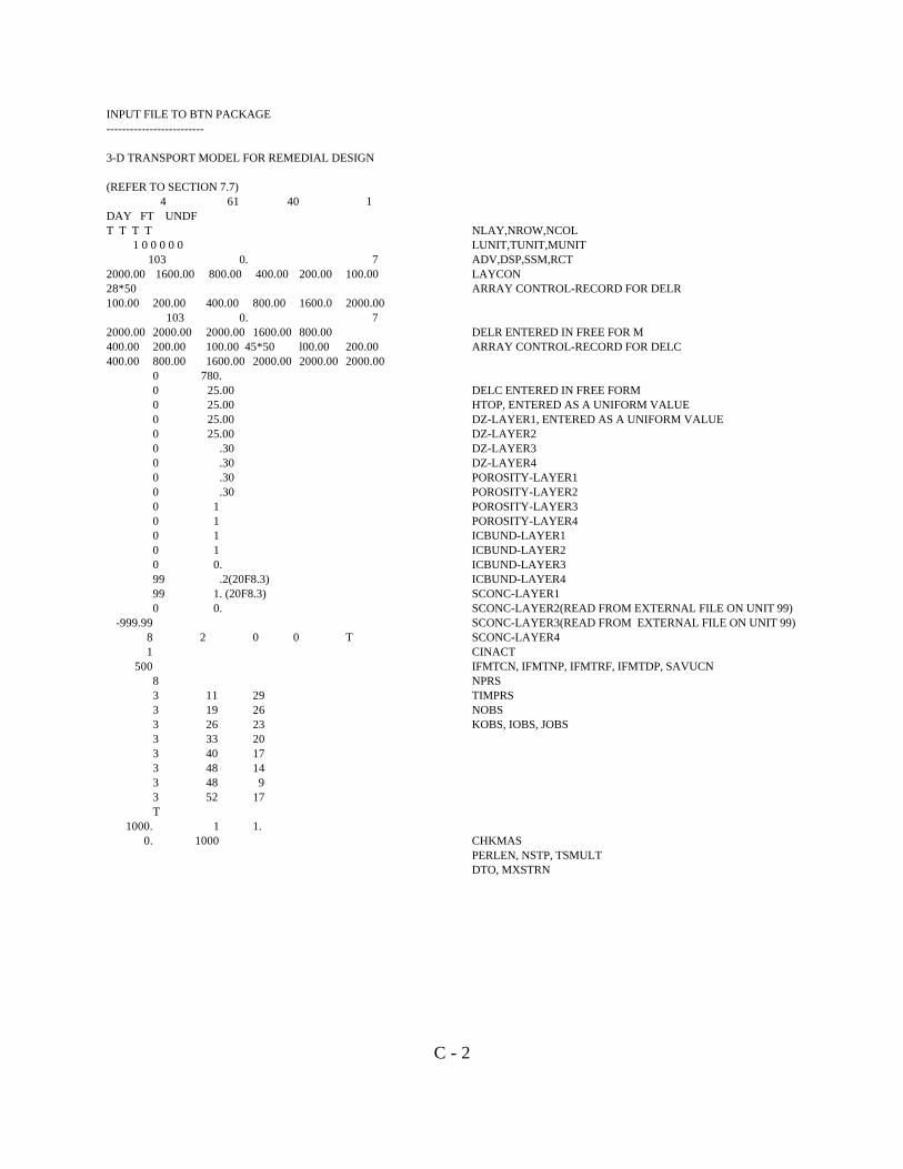
C - 2
INPUT FILE TO BTN PACKAGE-------------------------
3-D TRANSPORT MODEL FOR REMEDIAL DESIGN
(REFER TO SECTION 7.7)4 61 40 1
DAY FT UNDFT T T T
1 0 0 0 0 0103 0. 7
2000.00 1600.00 800.00 400.00 200.00 100.0028*50100.00 200.00 400.00 800.00 1600.0 2000.00
103 0. 72000.00 2000.00 2000.00 1600.00 800.00400.00 200.00 100.00 45*50 l00.00 200.00400.00 800.00 1600.00 2000.00 2000.00 2000.00
0 780.0 25.000 25.000 25.000 25.000 .300 .300 .300 .300 10 10 10 10 0.99 .2(20F8.3)99 1. (20F8.3)0 0.
-999.998 2 0 0 T1
50083 11 293 19 263 26 233 33 203 40 173 48 143 48 93 52 17T
1000. 1 1.0. 1000
NLAY,NROW,NCOLLUNIT,TUNIT,MUNITADV,DSP,SSM,RCTLAYCONARRAY CONTROL-RECORD FOR DELR
DELR ENTERED IN FREE FOR MARRAY CONTROL-RECORD FOR DELC
DELC ENTERED IN FREE FORMHTOP, ENTERED AS A UNIFORM VALUEDZ-LAYER1, ENTERED AS A UNIFORM VALUEDZ-LAYER2DZ-LAYER3DZ-LAYER4POROSITY-LAYER1POROSITY-LAYER2POROSITY-LAYER3POROSITY-LAYER4ICBUND-LAYER1ICBUND-LAYER2ICBUND-LAYER3 ICBUND-LAYER4SCONC-LAYER1SCONC-LAYER2(READ FROM EXTERNAL FILE ON UNIT 99)SCONC-LAYER3(READ FROM EXTERNAL FILE ON UNIT 99)SCONC-LAYER4CINACTIFMTCN, IFMTNP, IFMTRF, IFMTDP, SAVUCNNPRSTIMPRSNOBSKOBS, IOBS, JOBS
CHKMASPERLEN, NSTP, TSMULTDTO, MXSTRN
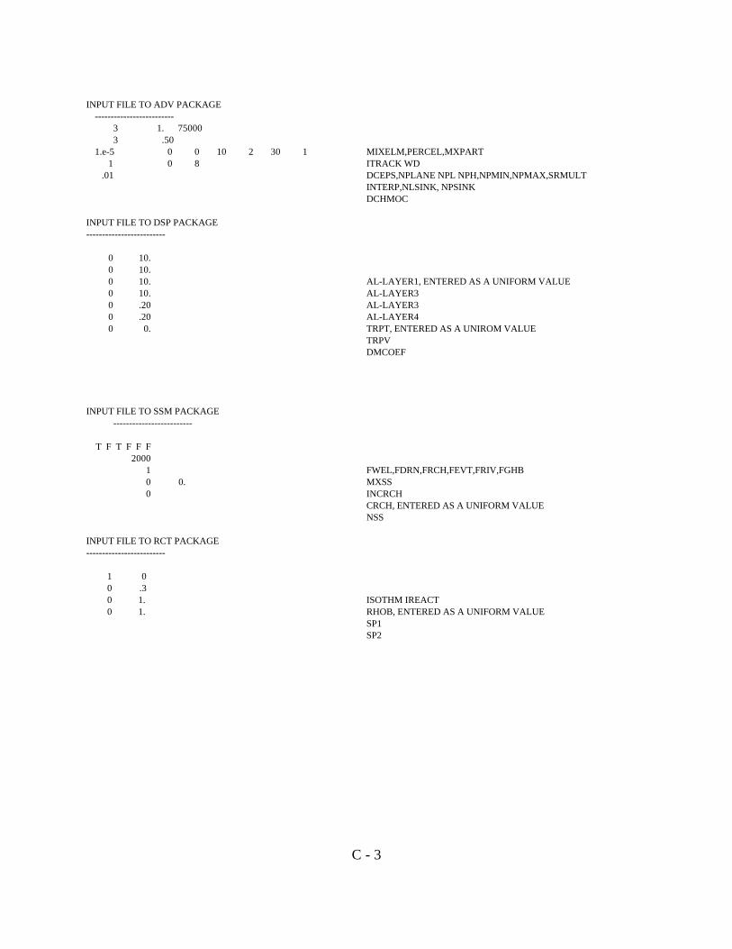
C - 3
INPUT FILE TO ADV PACKAGE-------------------------
3 1. 750003 .50
1.e-5 0 0 10 2 30 11 0 8
.01
INPUT FILE TO DSP PACKAGE-------------------------
0 10.0 10.0 10.0 10.0 .200 .200 0.
INPUT FILE TO SSM PACKAGE-------------------------
T F T F F F2000
10 0.0
INPUT FILE TO RCT PACKAGE-------------------------
1 00 .30 1.0 1.
MIXELM,PERCEL,MXPARTITRACK WDDCEPS,NPLANE NPL NPH,NPMIN,NPMAX,SRMULTINTERP,NLSINK, NPSINKDCHMOC
AL-LAYER1, ENTERED AS A UNIFORM VALUEAL-LAYER3AL-LAYER3AL-LAYER4TRPT, ENTERED AS A UNIROM VALUETRPVDMCOEF
FWEL,FDRN,FRCH,FEVT,FRIV,FGHBMXSSINCRCHCRCH, ENTERED AS A UNIFORM VALUENSS
ISOTHM IREACTRHOB, ENTERED AS A UNIFORM VALUESP1SP2

C - 4
M T 3 DA Modular Three-Dimensional Transport ModelFor Simulation of Advection, Dispersion and Chemical Reactionsof Contaminants in Groundwater Systems
M T 3-D TRANS MODEL F0R REMEDIAL DESIGN3 D (REFER TO SECTION 7.7)
THE TRANSPORT MODEL CONSISTS OF 4 LAYER(S) 61 ROW(S) 41 COLUMN(S)NUMBER OF STRESS PERI OD (S) I N SIMULA T ION = 1UNIT FOR TIME IS DAY ; UNIT FOR LENGTH IS FT ; UNIT FOR MASS IS UNDFM AJOR TRAANSPORT COMPONENTS TO BE SIMULATED:
1 ADVECTION2 DISPERSION3 SINK AND SOURCE MIXING4 CHEMICAL REACTIONS (DECAY AND/OR SORPTION)
BTN1 -- BASIC TRANPORT PACKAGE, VER 1.0, AUGUST 1990, INPUT READ FROM UNIT 1117322 ELEMENTS OF THE X ARRAY USED BY THE BTN PACKAGE 9764 ELEMENTS OF THE IX ARRAY USED BY THE BTN PACKAGE
ADV1 -- ADVECTION PACKAGE, VER 1.0, AUGUST 1990, INPUT READ FRO14 UNIT 2ADVECTION IS SOLVED WITH THE HYBRID [MOC]/ [MMOC] SCHEMECOURANT NUMBER ALLOWED IN SOLVING THE ADVECTION TERM = l.00MAXIMUM NUMBER OF MOVING PARTICLES ALLOWED = 75000
300000 ELEMENTS OF THE X ARRAY USED BY THE ADV PACKAGE 9760 ELEMENTS OF THE IX ARRAY USED BY THE ADV PACKAGE
DSP1 -- DISPERSION PACKAGE, VER 1.0, AUGUST 1990, INPUT READ FROM UNIT 397612 ELEMENTS OF THE X ARRAY USED BY THE DSP PACKAGE 0 ELEMENTS OF THE IX ARRAY USED BY THE DSP PACKAGE
SSM1 --SINK & SOURCE MIXING PACKAGE, VER 1.1 AUGUST 1990, INPUT READ FROM UNIT 4MAJOR STRESS COMPONENTS PRESENT IN THE FLOW MODEL:
1 WELL2 RECHARGE
MAXIMUM NUMBER OF POINT SINKS/SOURCES = 200016880 ELEMENTS OF THE X ARRAY USED BY THE SSM PACKAGE 2440 ELEMENTS OF THE IX ARRAY BY THE SSM PACKAGE
RCT1 -- CHEMICAL REACTIONS PACKAGE, VER 1.0, AUGUST 1990, INPUT READ FROM UNIT 9TYP E OF SORPTION SELECTED IS [LINEAR]NO FIRST-ORDER RATE REACTION IS SIMULATED
12 ELEMENTS OF THE X ARRAY USED BY THE RCT PACKAGE 0 ELEMENTS OF THE IX ARRAY USED BY THE RCT PACKAGE
............................................................531826 ELEMENTS OF THE X ARRAY USED OUT OF 800000 21964 ELEMENTS OF THE IX ARRAY USED OUT OF 80000............................................................LAYER NUMBER AQUIFER TYPE----------------------- ----------------------
1 12 03 04 0

C - 5
WIDTH ALONG ROWS (DELR) READ ON UNIT 1 USING FREE FORMAT---------------------------------------------------------------------------------------------------
1 2 3 4 5 6 7 8 9 10 11 12 13 14 15 16 17 18 19 2021 22 23 24 25 26 27 28 29 30 31 32 33 34 35 36 37 38 39 40
.....................................................................................................................................................................................................................1 2000. 1600. 800. 400. 200. 100. 50. 50. 50. 50. 50. 50. 50. 50. 50. 50. 50. 50. 50. 50.
50. 50. 50. 50. 50. 50. 50. 50. 50. 50. 50. 50. 50. 50. 100. 200. 400. 800. 1600. 2000.
WIDTH ALONG COLS (DELC) READ ON UNIT 1 USING FREE FORMAT-----------------------------------------------------------------------------------------------------
1 2 3 4 5 6 7 8 9 10 11 12 13 14 15 16 17 18 19 2021 22 23 24 25 26 27 28 29 30 31 32 33 34 35 36 37 38 39 4041 42 43 44 45 46 47 48 49 50 51 52 53 54 55 56 57 58 59 6061
..........................................................................................................................................................................................................1 2000. 2000.2000.1600. 800. 400. 200. 100. 50. 50. 50. 50. 50. 50. 50. 50. 50. 50. 50. 50.
50. 50. 50. 50. 50. 50. 50. 50. 50. 50. 50. 50. 50. 50. 50. 50. 50. 50. 50. 50.50. 50. 50. 50. 50. 50. 50. 50. 50. 50. 50. 50. 50. 100. 200. 400. 800. 1600. 2000. 2000.
2000.TOP ELEV. OF 1ST LAYER = 780.0000CELL THICKNESS (DZ) = 25.00000 FOR LAYER 1CELL THICKNESS (DZ) = 25.00000 FOR LAYER 2CELL THICKNESS (DZ) = 25.00000 FOR LAYER 3CELL THICKNESS (DZ) = 25.00000 FOR LAYER 4EFFECTIVE POROSITY = 0.3000000 FOR LAYER 1EFFECTIVE POROSITY = 0.3000000 FOR LAYER 2EFFECTIVE POROSITY = 0.3000000 FOR LAYER 3EFFECTIVE POROSITY = 0.3000000 FOR LAYER 4CONCN. BOUNDARY ARRAY= 1 FOR LAYER 1CONCN. BOUNDARY ARRAY= 1 FOR LAYER 2CONCN. BOUNDARY ARRAY= 1 FOR LAYER 3CONCN. BOUNDARY ARRAY= 1 FOR LAYER 4INITIAL CONCENTRATION = 0.0000000 FOR LAYER 1
INITIAL CONCENTRATION FOR LAYER 2 READ ON UNIT 99 USING FORMAT: "(20F8.3) "-----------------------------------------------------------------------------------------------------------------------------------------INITIAL CONCENTRATION FOR LAYER 3 READ ON UNIT 99 USING FORMAT: "(20F8.3) "-----------------------------------------------------------------------------------------------------------------------------------------
INITIAL CONCENTRATION = 0.0000000 FOR LAYER 4
VALUE INDICATING INACTIVE CONCENTRATION CELLS = -999.9900
OUPUT CONTROL OPTIONS----------------------PRINT CELL CONCENTRATION USING FORMAT CODE: 8PRINT PARTICLE NUMBER IN EACH CELL USING FORMAT CODE: 2PRINT RETRDATION FACTOR USING FORMAT CODE: 0DO NOT PRINT DISPERSION COEFFICIENTSAVE CONCENTRATION IN UNFORMATED FILE [MT3D.UCN] ON UNIT 18
NUMBER OF TIMES AT WHICH SIMULATION RESULT ARE SAVED = 1TOTAL ELAPSED TIMES AT WHICH SIMULATION RESULTS ARE SAVED:
500.00

C - 6
NUMBER OF OBSERVATION POINTS = 8CONCENTRATION AT OBSERVATION POINTS SAVED IN FILE [MT3D.OBS] ON UNIT 17LOCATION OF OBSERVATION POINTS.....................................................................NUMBER LAYER ROW COLUMN
1 3 11 292 3 19 263 3 26 234 3 33 205 3 40 176 3 48 147 3 48 98 3 52 17
A ONE-LINE SUMMRY OF MASS BALANCE FOR EACH STEP SAVED IN FILE [MT3D.MAS] ON UNIT 19
MAXIMUM LENGTH ALONG THE X (J) AXIS = 11600.00MAXIMUM LENGTH ALONG THE Y (I) AXIS = 20450.00MAXIMUM LENGTH ALONG THE Z (K) AXIS = 100.0000
ADVECTION SOLUTION OPTIONS-----------------------------------------------
METHOD FOR PARTICLE TRACKING IS [MIXED ORDER]CONCENTRATION WEIGHTING FACTOR = 0.5 00THE CONCENTRATION GRADIIENT CONSIDERED NEGLIGIBLE [DCEPS] = 0.1000000E-04INITIAL PARTICLES ARE PLACED RANDOMLY WITHIN CELL BLOCKPARTICLE NUMBER PER CELL IF DCCELL =< DCEPS = 0PARTICLE NUMBER PER CELL IF DCCELL > DCEPS = 10MINIMUM PARTICLE NUMBER ALLOWD PER CELL = 2MAXIMUM PARTICLE NUMBER ALLOWD PER CELL = 30MULTIPLIER OF PARTICLE NUMBER AT SOURCE = 1.00SCHEME FOR CONCENTRATION INTERPOLATION IS [LINEAR]PARTICLES FOR APPROXIMATING A SINK CELL IN THE [MMOC] SCHEMEARE PLACED RANDOMLY WITHIN CELL BLOCKNUMBER OF PARTICLES USED TO APPROXIMATE A SINK CELL IN THE [MMOC] SCHEME = 8CRITICAL CONCENTRATION GRADIENT USED IN THE "HMOC" SCHEME [DCHMOC]= 0.1000E-01THE "MOC" SOLUTION IS USED WHEN DCCELL > DCHMOCTHE "MMOC" SOLUTION IS USED WHEN DCCELL =< DCHMOC
DISPERSION PARAMETERS--------------------------------------
LONG. DISPERSIVITY (AL) = 10.00000 FOR LAYER 1LONG. DISPERSIVITY (AL) = 10.00000 FOR LAYER 2LONG. DISPERSIVITY (AL) = 110.00000 FOR LAYER 3LONG. DISPERSIVITY (AL) = 110.00000 FOR LAYER 1H. TRANS./LONG. DISP = 0.2000000V. TRANS./LONG. DISP = 0.2000000DIFFUSION COEFFICIENT = 0.0000000
SORPTION AND 1ST ORDER RATE REACTION PARAMETERS------------------------------------------------------------------------------------
BULK DENSITY (RHOB) = 0.3000000SORPTION CONSTANT NO.1 = 1.000000SORPTION CONSTANT NO.2 = 1.000000

C - 7
STRESS PERIOD NO. 001
LENGTH OF CURRENT STRESS PERIOD = 1000.000NUMBER OF TIME STEPS FOR CURRENT STRESS PERIOD = 1TIME STEP MULTIPLIER = 1.000000USER-SPECIFIEDTRANSPORT STEPSIZE = 0.0000000 DAYMAXIMUM NUMBER OF TRANSPORT STEP ALLOWED IN ONE TIME STEP = 1000
CONCENTRATION OF RECHARGE FLUXES WILL BE READ IN STRESS PERIOD 1CONC. OF RECH. FLUX = 0.0000000
NO. OF POINT SINKS/SOURCES OF SPECIFIED CONCONCENTRATIONS = 0 IN STRESS PERIOD 1
--------------------------TIME STEP NO. 001--------------------------
FROM TIME = 0.00000 To 1000.0
"HEAD " FLOW TERMS FOR TIME STEP 1, STRESS PERIOD 1 READ UNFORMATTED ON UNIT 10---------------------------------------------------------------------------------------------------------------------------------------------------"QXX " FLOW TERMS FOR TIME STEP 1, STRESS PERIOD 1 READ UNFORMATTED ON UNIT 10---------------------------------------------------------------------------------------------------------------------------------------------------"QYY " FLOW TERMS FOR TIME STEP 1, STRESS PERIOD 1 READ UNFORMATTED ON UNIT 10---------------------------------------------------------------------------------------------------------------------------------------------------"QZZ " FLOW TERMS FOR TIME STEP 1, STRESS PERIOD 1 READ UNFORMATTED ON UNIT 10---------------------------------------------------------------------------------------------------------------------------------------------------
MAXIMUM STEPSIZE DURING WHICH ANY PARTICLE CANNOT MOVE MORE THAN ONE CELL = 4.822 (WHEN MIN. R.R. = 1) AT K= 3, I= 10, J= 29
"CNH " FLOW TERMS FOR TIME STEP 1, STRESS PERIOD 1 READ UNFORMATTED ON UNIT 10---------------------------------------------------------------------------------------------------------------------------------------------------"WEL " FLOW TERMS FOR TIME STEP 1, STRESS PERIOD 1 READ UNFORMATTED ON UNIT 10---------------------------------------------------------------------------------------------------------------------------------------------------"RCH " FLOW TERMS FOR TIME STEP 1, STRESS PERIOD 1 READ UNFORMATTED ON UNIT 10---------------------------------------------------------------------------------------------------------------------------------------------------
TOTAL NUMBER OF POINT SOtJRCES/SINKS PRESENT IN THE FLOW MODEL = 800
MAXIMUM STEPSIZE WHICH MEETS STABILITY CRITERION OF THE SINK & SOURCE TERM= 558.2 ( WHEN MIN. R.F.= 1) AT K = 4, I = 1, J = 7
MAXIMUM STEPSIZE WHICH MEETS STABILITY CRITERION OF THE DISPERSION TERM= 3.959 (WHEN MIN. R.F.=l) AT K = 3, I = 48, J = 14
-------------------------------------------TRANSPORT STEP No. 64-------------------------------------------TOTAL ELAPSED TIME SINCE BEGINNING OF SIMULATION = 500.0000 DAY .....................................................................
CONCENTRATIONS IN LAYER 1 AT END OF TRANSPORT STEP 64, TIME STEP 1, STRESS PERIOD 1------------------------------- -------------------------------------------------------CONCENTRATIONS IN LAYER 2 AT END OF TRANSPORT STEP 64, TIME STEP 1, STRESS PERIOD 1 -------------- -- ----- - -- --- -- --------- ---- ----------------------------------CONCENTRATIONS IN LAYER 3 AT END OF TRANSPORT STEP 64, TIME STEP 1, STRESS PERIOD 1 ------------------------------------------------------------------------------------------CONCENTRATIONS IN LAYER 4 AT END OF TRANSPORT STEP 64, TIME STEP 1, STRESS PERIOD 1 ------------------------------------------------------------------------------------------
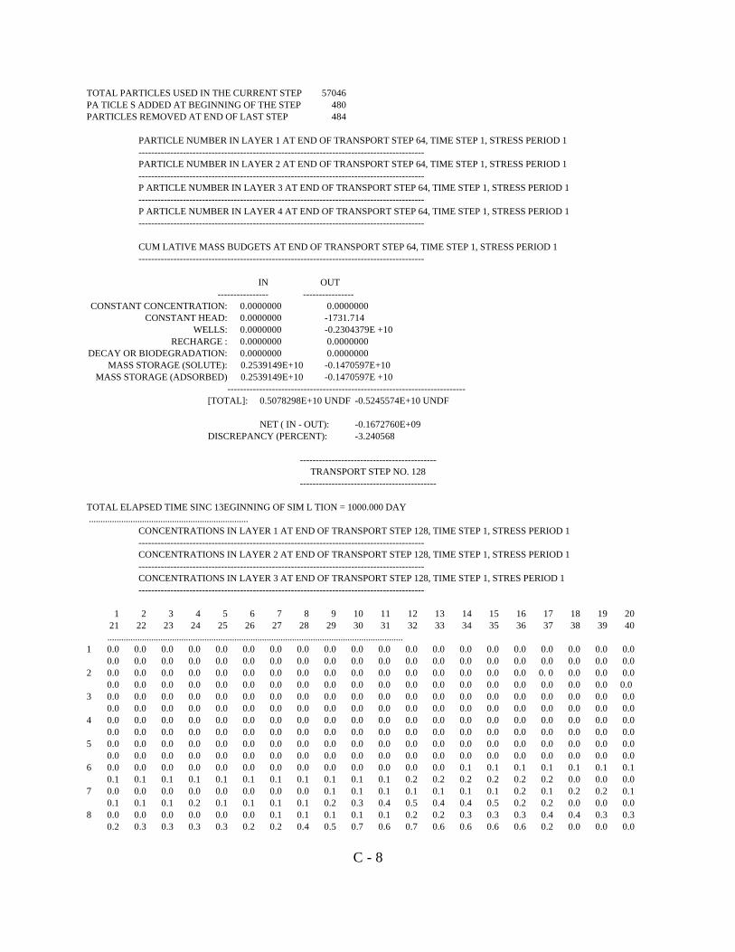
C - 8
TOTAL PARTICLES USED IN THE CURRENT STEP 57046PA TICLE S ADDED AT BEGINNING OF THE STEP 480PARTICLES REMOVED AT END OF LAST STEP 484
PARTICLE NUMBER IN LAYER 1 AT END OF TRANSPORT STEP 64, TIME STEP 1, STRESS PERIOD 1 ------------------------------------------------------------------------------------------PARTICLE NUMBER IN LAYER 2 AT END OF TRANSPORT STEP 64, TIME STEP 1, STRESS PERIOD 1 ------------------------------------------------------------------------------------------P ARTICLE NUMBER IN LAYER 3 AT END OF TRANSPORT STEP 64, TIME STEP 1, STRESS PERIOD 1 ------------------------------------------------------------------------------------------P ARTICLE NUMBER IN LAYER 4 AT END OF TRANSPORT STEP 64, TIME STEP 1, STRESS PERIOD 1 ------------------------------------------------------------------------------------------
CUM LATIVE MASS BUDGETS AT END OF TRANSPORT STEP 64, TIME STEP 1, STRESS PERIOD 1 ------------------------------------------------------------------------------------------
IN OUT---------------- ----------------
CONSTANT CONCENTRATION: 0.0000000 0.0000000CONSTANT HEAD: 0.0000000 -1731.714
WELLS: 0.0000000 -0.2304379E +10RECHARGE : 0.0000000 0.0000000
DECAY OR BIODEGRADATION: 0.0000000 0.0000000MASS STORAGE (SOLUTE): 0.2539149E+10 -0.1470597E+10
MASS STORAGE (ADSORBED) 0.2539149E+10 -0.1470597E +10---------------------------------------------------------------------------
[TOTAL]: 0.5078298E+10 UNDF -0.5245574E+10 UNDF
NET ( IN - OUT): -0.1672760E+09DISCREPANCY (PERCENT): -3.240568
-------------------------------------------TRANSPORT STEP NO. 128
-------------------------------------------
TOTAL ELAPSED TIME SINC 13EGINNING OF SIM L TION = 1000.000 DAY .....................................................................
CONCENTRATIONS IN LAYER 1 AT END OF TRANSPORT STEP 128, TIME STEP 1, STRESS PERIOD 1 ------------------------------------------------------------------------------------------CONCENTRATIONS IN LAYER 2 AT END OF TRANSPORT STEP 128, TIME STEP 1, STRESS PERIOD 1 ------------------------------------------------------------------------------------------CONCENTRATIONS IN LAYER 3 AT END OF TRANSPORT STEP 128, TIME STEP 1, STRES PERIOD 1------------------------------------------------------------------------------------------
1 2 3 4 5 6 7 8 9 10 11 12 13 14 15 16 17 18 19 2021 22 23 24 25 26 27 28 29 30 31 32 33 34 35 36 37 38 39 40
................................................................................................................................1 0.0 0.0 0.0 0.0 0.0 0.0 0.0 0.0 0.0 0.0 0.0 0.0 0.0 0.0 0.0 0.0 0.0 0.0 0.0 0.0
0.0 0.0 0.0 0.0 0.0 0.0 0.0 0.0 0.0 0.0 0.0 0.0 0.0 0.0 0.0 0.0 0.0 0.0 0.0 0.02 0.0 0.0 0.0 0.0 0.0 0.0 0.0 0.0 0.0 0.0 0.0 0.0 0.0 0.0 0.0 0.0 0. 0 0.0 0.0 0.0
0.0 0.0 0.0 0.0 0.0 0.0 0.0 0.0 0.0 0.0 0.0 0.0 0.0 0.0 0.0 0.0 0.0 0.0 0.0 0.0 3 0.0 0.0 0.0 0.0 0.0 0.0 0.0 0.0 0.0 0.0 0.0 0.0 0.0 0.0 0.0 0.0 0.0 0.0 0.0 0.0
0.0 0.0 0.0 0.0 0.0 0.0 0.0 0.0 0.0 0.0 0.0 0.0 0.0 0.0 0.0 0.0 0.0 0.0 0.0 0.04 0.0 0.0 0.0 0.0 0.0 0.0 0.0 0.0 0.0 0.0 0.0 0.0 0.0 0.0 0.0 0.0 0.0 0.0 0.0 0.0
0.0 0.0 0.0 0.0 0.0 0.0 0.0 0.0 0.0 0.0 0.0 0.0 0.0 0.0 0.0 0.0 0.0 0.0 0.0 0.05 0.0 0.0 0.0 0.0 0.0 0.0 0.0 0.0 0.0 0.0 0.0 0.0 0.0 0.0 0.0 0.0 0.0 0.0 0.0 0.0
0.0 0.0 0.0 0.0 0.0 0.0 0.0 0.0 0.0 0.0 0.0 0.0 0.0 0.0 0.0 0.0 0.0 0.0 0.0 0.06 0.0 0.0 0.0 0.0 0.0 0.0 0.0 0.0 0.0 0.0 0.0 0.0 0.0 0.1 0.1 0.1 0.1 0.1 0.1 0.1
0.1 0.1 0.1 0.1 0.1 0.1 0.1 0.1 0.1 0.1 0.1 0.2 0.2 0.2 0.2 0.2 0.2 0.0 0.0 0.07 0.0 0.0 0.0 0.0 0.0 0.0 0.0 0.0 0.1 0.1 0.1 0.1 0.1 0.1 0.1 0.2 0.1 0.2 0.2 0.1
0.1 0.1 0.1 0.2 0.1 0.1 0.1 0.1 0.2 0.3 0.4 0.5 0.4 0.4 0.5 0.2 0.2 0.0 0.0 0.08 0.0 0.0 0.0 0.0 0.0 0.0 0.1 0.1 0.1 0.1 0.1 0.2 0.2 0.3 0.3 0.3 0.4 0.4 0.3 0.3
0.2 0.3 0.3 0.3 0.3 0.2 0.2 0.4 0.5 0.7 0.6 0.7 0.6 0.6 0.6 0.6 0.2 0.0 0.0 0.0

C - 9
9 0.0 0.0 0.0 0.0 0.0 0.0 0.1 0.1 0.2 0.2 0.2 0.3 0.3 0.4 0.4 0.4 0.5 0.5 0.5 0.60.4 0.4 0.4 0.4 0.3 0.3 0.4 0.5 0.6 0.8 1.0 0.9 0.8 0.6 0.7 0.7 0.3 0.0 0.0 0.0
10 0.0 0.0 0.0 0.0 0.0 0.0 0.1 0.1 0.2 0.2 0.3 0.4 0.5 0.5 0.5 0.7 0.6 0.8 0.6 0.80.6 0.6 0.6 0.5 0.5 0.5 0.4 0.6 0.7 1.1 1.1 1.2 1.1 0.9 0.8 0.8 0.4 0.0 0.0 0.0
11 0.0 0.0 0.0 0.0 0.0 0.1 0.1 0.2 0.2 0.3 0.4 0.4 0.6 0.6 0.7 0.8 0.8 0.8 0.8 0.90.7 0.8 0.8 0.8 0.6 0.7 0.7 0.9 1.1 1.2 1.5 1.2 1.3 1.2 1.1 1.0 0.5 0.0 0.0 0.0
12 0.0 0.0 0.0 0.0 0.0 0.1 0.1 0.2 0.3 0.4 0.4 0.6 0.7 0.8 0.9 1.3 1.3 1.1 1.1 1.21.0 1.2 1.0 1.0 0.9 1.3 1.1 0.8 1.5 2.1 1.7 1.3 1.5 1.4 1.2 1.1 0.5 0.0 0.0 0.0
13 0.0 0.0 0.0 0.0 0.0 0.1 0.2 0.3 0.4 0.4 0.6 0.8 0.9 1.0 1.2 1.5 1.4 1.4 1.5 1.51.4 1.4 1.4 1.3 1.3 1.5 1.4 1.9 2.5 2.7 2.2 1.9 1.8 1.6 1.5 1.3 0.6 0.0 0.0 0.0
14 0.0 0.0 0.0 0.0 0.0 0.1 0.3 0.4 0.5 0.6 0.8 1.0 1.1 1.3 1.5 1.7 1.7 1.8 2.4 1.81.7 1.7 1.7 1.8 1.8 2.4 2.4 2.8 2.7 3.1 2.9 2.4 2.1 1.9 1.8 1.8 0.6 0.0 0.0 0.0
15 0.0 0.0 0.0 0.0 0.0 0.2 0.4 0.5 0.7 0.8 1.0 1.1 1.4 1.6 1.9 2.2 2.1 2.2 2.3 2.32.2 2.9 2.3 2.5 2.5 2.8 3.9 4.2 3.8 3.6 3.0 2.7 2.5 2.2 1.9 1.5 0.6 0.0 0.0 0.0
16 0.0 0.0 0.0 0.0 0.0 0.3 0.5 0.6 1.0 0.9 1.2 1.4 1.7 1.8 2.2 2.8 2.6 2.6 2.8 2.62.8 2.8 2.9 3.0 2.9 4.1 5.2 5.1 5.0 4.7 3.5 3.3 2.7 2.7 2.1 1.5 0.7 0.0 0.0 0.0
17 0.0 0.0 0.0 0.0 0.1 0.3 0.6 0.8 1.0 1.3 1.5 1.7 2.1 2.3 2.6 3.1 3.2 3.1 3.4 4.03.7 3.3 3.4 3.8 3.5 4.1 6.5 5.5 6.0 4.7 4.6 3.8 3.4 2.8 2.6 1.9 0.7 0.0 0.0 0.0
18 0.0 0.0 0.0 0.0 0.1 0.4 0.7 1.0 1.2 1.5 1.8 2.2 2.5 2.8 3.2 3.5 3.8 3.7 4.0 4.24.0 5.0 4.2 4.5 4.4 5.2 6.4 6.1 5.8 5.2 4.9 4.3 3.6 3.5 2.7 1.9 0.8 0.0 0.0 0.0
19 0.0 0.0 0.0 0.0 0.1 0.5 0.9 1.2 1.5 2.0 2.2 2.5 3.0 3.4 3.8 4.0 4.4 4.6 4.8 5.04.9 5.1 5.2 4.5 4.4 6.8 8.1 6.4 6.5 5.9 5.1 4.4 4.2 3.3 2.9 2.0 0.7 0.0 0.0 0.0
20 0.0 0.0 0.0 0.0 0.1 0.6 1.0 1.4 1.7 2.2 2.7 3.0 3.5 4.2 4.8 4.5 5.2 5.4 5.8 5.86.2 5.8 6.6 5.8 5.2 7.6 7.9 7.6 6.8 6.3 5.2 4.6 4.1 3.8 3.4 2.0 0.6 0.0 0.0 0.0
21 0.0 0.0 0.0 0.0 0.2 0.7 1.3 1.7 2.2 2.6 3.3 3.6 3.7 4.7 5.0 5.8 6.3 6.4 6.7 6.56.9 6.8 7.9 6.3 11.7 9.3 8.9 8.0 7.3 6.8 5.8 5.0 4.5 4.2 3.6 1.9 0.7 0.0 0.0 0.0
22 0.0 0.0 0.0 0.0 0.2 0.9 1.5 2.0 2.5 3.0 3.5 4.2 5.0 6.7 6.0 6.5 6.5 7.5 7.6 8.27.8 8.2 7.1 9.0 11.7 10.9 10.0 8.6 7.7 7.0 6.1 5.4 4.6 4.1 3.8 2.1 0.7 0.0 0.0 0.0
23 0.0 0.0 0.0 0.0 0.3 1.1 1.8 2.2 2.9 3.5 4.2 5.1 5.5 6.4 6.5 7.1 7.7 8.3 8.8 9.38.5 9.5 9.5 11.4 13.5 11.5 10.3 9.0 8.1 7.2 6.5 5.6 4.8 4.4 3.9 2.1 0.6 0.0 0.0 0.0
24 0.0 0.0 0.0 0.0 0.4 1.3 2.1 2.7 3.3 4.1 4.6 5.7 6.4 7.2 8.0 8.8 8.4 9.6 10.0 10.311.0 11.2 11.1 12.3 12.3 11.4 11.7 9.5 8.4 7.6 6.8 6.1 5.2 4.6 3.7 2.5 0.6 0.0 0.0 0.0
25 0.0 0.0 0.0 0.0 0.4 1.5 2.5 3.2 3.9 4.6 6.0 6.4 7.1 8.6 8.4 10.3 11.1 10.7 11.6 11.311.4 11.5 12.0 16.3 13.5 13.1 10.5 9.9 8.8 7.9 7.2 6.2 5.2 5.1 4.3 2.0 0.6 0.0 0.0 0.0
26 0.0 0.0 0.0 0.0 0.5 1.8 2.8 3.6 4.2 5.7 6.1 7.2 8.5 9.0 9.9 11.0 11.9 12.2 13.0 13.213.6 14.2 13.0 14.5 13.2 12.4 11.5 9.9 8.9 8.3 7.3 6.4 5.6 4.8 4.1 2.5 0.6 0.0 0.0 0.0
27 0.0 0.0 0.0 0.1 0.6 2.1 3.0 3.8 5.4 6.1 7.6 8.2 9.4 10.3 11.1 12.0 13.2 13.7 14.6 15.114.6 14.5 15.2 14.4 13.5 12.4 11.6 9.8 9.5 8.0 7.3 6.5 4.9 4.2 3.0 2.4 0.4 0.0 0.0 0.0
28 0.0 0.0 0.0 0.1 0.7 2.3 3.5 4.6 5.8 6.8 8.1 9.4 10.0 10.9 12.7 14.5 14.7 15.8 16.2 19.016.6 18.8 16.5 14.5 14.2 12.1 11.6 9.6 8.7 7.7 6.8 6.0 4.5 4.2 3.3 1.2 0.1 0.0 0.0 0.0
29 0.0 0.0 0.0 0.1 0.8 2.7 4.1 5.4 6.5 7.7 9.0 9.8 11.3 12.6 14.2 14.7 16.3 17.4 17.5 20.821.8 21.7 17.3 14.5 13.3 12.9 10.7 9.8 8.6 7.2 6.2 5.3 4.7 3.5 2.6 1.2 0.3 0.0 0.0 0.0
30 0.0 0.0 0.0 0.1 0.8 2.6 4.5 5.4 7.4 8.5 10.1 11.2 12.6 14.4 15.5 16.9 20.4 19.0 20.3 20.521.7 19.1 17.6 14.3 13.2 11.5 10.8 9.3 7.8 6.9 6.0 5.0 4.4 3.4 2.5 1.2 0.1 0.0 0.0 0.0
31 0.0 0.0 0.0 0.1 1.0 2.7 4.9 6.5 7.8 10.4 11.6 12.5 14.4 15.6 17.0 18.7 19.9 21.8 21.4 22.622.2 19.8 15.8 13.9 12.0 10.8 9.5 8.3 7.1 6.2 5.1 4.8 3.8 3.1 2.4 0.8 0.1 0.0 0.0 0.0
32 0.0 0.0 0.0 0.1 1.1 2.8 5.5 7.0 8.9 9.9 11.3 13.1 15.3 17.2 18.2 19.4 21.3 21.7 23.3 22.519.9 16.8 14.8 12.9 11.0 9.9 8.5 7.5 6.4 5.5 4.9 4.2 3.1 2.7 2.2 1.0 0.1 0.0 0.0 0.0
33 0.0 0.0 0.0 0.1 1.1 3.7 6.6 7.2 9.0 10.8 13.1 14.4 16.9 17.4 19.8 22.0 22.2 23.0 23.8 21.117.5 15.7 13.9 12.5 10.7 9.2 8.0 6.8 5.7 4.9 4.2 3.2 2.5 2.4 1.5 0.4 0.1 0.0 0.0 0.0
34 0.0 0.0 0.0 0.1 1.4 3.5 5.9 7.7 9.8 12.0 13.6 15.3 16.9 19.4 20.9 22.4 23.7 25.3 25.6 15.915.4 14.0 14.0 11.2 9.5 8.0 6.8 5.9 5.0 4.0 3.5 2.7 2.2 1.3 1.1 0.4 0.1 0.0 0.0 0.0
35 0.0 0.0 0.0 0.1 1.3 4.4 6.5 7.9 10.3 12.5 14.4 16.3 18.5 20.3 21.8 23.7 25.8 28.1 26.4 17.714.5 12.7 11.8 10.3 8.2 7.1 6.1 5.1 4.3 3.5 2.5 1.6 1.4 1.2 0.4 0.3 0.1 0.0 0.0 0.0
36 0.0 0.0 0.0 0.1 1.6 4.6 6.3 8.7 11.1 12.8 15.0 17.0 19.2 21.2 23.2 25.9 27.4 28.5 21.4 15.813.9 12.3 10.3 8.8 7.7 6.6 5.8 4.5 3.6 2.6 2.2 1.5 1.1 0.8 0.5 0.2 0.1 0.0 0.0 0.0
37 0.0 0.0 0.0 0.1 1.8 5.3 6.8 8.9 11.1 13.3 15.2 17.6 20.3 21.8 24.6 26.7 29.2 28.7 21.0 15.413.2 11.1 10.0 7.9 7.0 5.7 4.7 3.6 3.0 2.1 1.6 1.1 0.7 0.6 0.4 0.1 0.1 0.0 0.0 0.0
38 0.0 0.0 0.0 0.1 1.8 4.2 7.0 8.4 10.8 13.3 16.0 18.2 21.0 22.8 24.8 27.2 29.7 26.6 17.7 14.513.2 10.3 9.3 7.6 6.2 5.0 3.9 3.1 2.2 1.7 1.1 0.8 0.5 0.4 0.2 0.1 0.1 0.0 0.0 0.0
39 0.0 0.0 0.0 0.1 2.2 4.4 7.3 8.5 11.5 14.0 16.4 18.4 20.6 23.5 26.0 27.6 27.7 21.9 15.7 13.712.1 9.7 8.3 7.1 5.6 4.5 3.4 2.4 1.8 1.4 1.0 0.6 0.4 0.3 0.2 0.1 0.0 0.0 0.0 0.0

C - 10
40 0.0 0.0 0.0 0.1 2.4 3.4 7.4 8.6 11.1 13.7 16.1 18.9 20.8 22.9 25.4 24.7 23.2 16.3 14.5 12.311.0 9.0 7.5 6.0 5.0 3.7 2.7 2.1 1.8 1.1 0.6 0.4 0.3 0.2 0.1 0.1 0.0 0.0 0.0 0.0
41 0.0 0.0 0.0 0.1 2.2 3.4 7.4 8.9 10.9 14.0 16.7 18.6 21.3 23.4 24.2 25.9 18.1 13.4 12.4 11.19.3 7.9 7.0 5.3 4.1 3.0 2.2 1.7 1.2 0.7 0.6 0.4 0.3 0.1 0.1 0.1 0.0 0.0 0.0 0.0
42 0.0 0.0 0.0 0.1 2.2 3.6 7.2 8.4 11.5 13.7 16.1 18.8 21.8 23.3 26.1 24.0 14.3 12.0 11.0 9.88.3 7.0 5.7 4.5 3.2 2.4 1.8 1.1 0.9 0.6 0.4 0.3 0.2 0.1 0.1 0.1 0.0 0.0 0.0 0.0
43 0.0 0.0 0.0 0.0 1.4 3.4 7.1 8.0 10.2 13.1 16.1 19.0 21.5 23.7 24.6 19.5 12.4 11.2 9.8 8.97.3 6.3 4.8 3.7 2.6 2.0 1.4 1.1 0.7 0.5 0.3 0.2 0.1 0.1 0.1 0.0 0.0 0.0 0.0 0.0
44 0.0 0.0 0.0 0.0 1.1 3.3 4.9 7.9 9.9 12.8 15.8 18.9 21.8 24.0 24.7 15.3 12.1 10.2 8.9 7.86.2 4.9 3.9 3.1 2.2 1.7 1.1 0.8 0.5 0.4 0.3 0.2 0.1 0.1 0.1 0.0 0.0 0.0 0.0 0.0
45 0.0 0.0 0.0 0.0 1.2 2.9 4.2 6.9 9.4 12.6 15.8 19.0 22.0 24.3 22.3 14.2 11.0 9.5 8.1 6.15.0 4.1 3.2 2.5 1.7 1.2 0.9 0.6 0.4 0.3 0.2 0.1 0.1 0.1 0.1 0.0 0.0 0.0 0.0 0.0
46 0.0 0.0 0.0 0.0 0.9 2.6 3.1 4.6 8.3 12.1 15.5 18.5 22.1 24.0 19.1 12.6 9.9 8.0 6.5 5.24.2 3.4 2.6 1.7 1.2 0.9 0.7 0.4 0.3 0.2 0.2 0.1 0.1 0.1 0.0 0.0 0.0 0.0 0.0 0.0
47 0.0 0.0 0.0 0.0 0.4 1.9 2.6 4.0 8.0 11.9 15.3 18.0 21.4 21.5 13.7 11.2 8.1 6.9 5.2 4.23.0 2.4 1.9 1.5 1.1 0.6 0.5 0.3 0.2 0.2 0.1 0.1 0.1 0.1 0.0 0.0 0.0 0.0 0.0 0.0
48 0.0 0.0 0.0 0.0 0.2 1.2 1.9 2.4 6.3 11.9 15.0 16.6 16.7 14.9 10.4 8.5 7.8 5.5 4.2 3.32.4 1.8 1.2 1.0 0.6 0.4 0.3 0.2 0.1 0.1 0.1 0.1 0.1 0.0 0.0 0.0 0.0 0.0 0.0 0.0
49 0.0 0.0 0.0 0.0 0.2 0.7 0.7 1.0 1.8 6.0 12.7 13.8 12.3 9.5 7.9 7.4 5.5 4.2 3.2 2.31.8 1.3 0.9 0.6 0.5 0.3 0.2 0.2 0.1 0.1 0.1 0.1 0.0 0.0 0.0 0.0 0.0 0.0 0.0 0.0
50 0.0 0.0 0.0 0.0 0.1 0.2 0.3 0.3 0.7 1.1 3.0 4.9 5.5 6.7 7.3 6.2 4.3 3.0 2.2 1.51.0 0.8 0.6 0.4 0.3 0.2 0.2 0.1 0.1 0.1 0.1 0.0 0.0 0.0 0.0 0.0 0.0 0.0 0.0 0.0
51 0.0 0.0 0.0 0.0 0.1 0.1 0.2 0.3 0.3 1.0 2.3 3.5 3.6 4.3 6.4 5.6 3.1 2.2 1.2 0.80.6 0.5 0.3 0.3 0.2 0.2 0.1 0.1 0.1 0.1 0.0 0.0 0.0 0.0 0.0 0.0 0.0 0.0 0.0 0.0
52 0.0 0.0 0.0 0.0 0.1 0.1 0.1 0.2 0.3 0.9 1.8 3.9 2.7 3.0 5.1 3.1 1.7 0.9 0.6 0.50.4 0.3 0.2 0.2 0.2 0.1 0.1 0.1 0.1 0.0 0.0 0.0 0.0 0.0 0.0 0.0 0.0 0.0 0.0 0.0
53 0.0 0.0 0.0 0.0 0.1 0.1 0.1 0.2 0.3 0.8 2.5 4.2 2.7 2.1 1.2 1.0 0.4 0.4 0.3 0.30.2 0.2 0.2 0.2 0.1 0.1 0.1 0.1 0.0 0.0 0.0 0.0 0.0 0.0 0.0 0.0 0.0 0.0 0.0 0.0
54 0.0 0.0 0.0 0.0 0.0 0.1 0.1 0.2 0.5 1.8 3.4 3.7 3.2 0.8 0.2 0.2 0.2 0.2 0.2 0.20.1 0.1 0.1 0.1 0.1 0.1 0.0 0.0 0.0 0.0 0.0 0.0 0.0 0.0 0.0 0.0 0.0 0.0 0.0 0.0
55 0.0 0.0 0.0 0.0 0.0 0.1 0.1 0.3 1.1 1.3 0.9 0.7 0.2 0.1 0.1 0.1 0.1 0.1 0.1 0.10.1 0.0 0.0 0.0 0.0 0.0 0.0 0.0 0.0 0.0 0.0 0.0 0.0 0.0 0.0 0.0 0.0 0.0 0.0 0.0
56 0.0 0.0 0.0 0.0 0.0 0.1 0.1 0.2 0.3 0.2 0.2 0.2 0.2 0.1 0.0 0.0 0.0 0.0 0.0 0.00.0 0.0 0.0 0.0 0.0 0.0 0.0 0.0 0.0 0.0 0.0 0.0 0.0 0.0 0.0 0.0 0.0 0.0 0.0 0.0
57 0.0 0.0 0.0 0.0 0.0 0.0 0.0 0.1 0.1 0.1 0.1 0.1 0.0 0.0 0.0 0.0 0.0 0.0 0.0 0.00.0 0.0 0.0 0.0 0.0 0.0 0.0 0.0 0.0 0.0 0.0 0.0 0.0 0.0 0.0 0.0 0.0 0.0 0.0 0.0
58 0.0 0.0 0.0 0.0 0.0 0.0 0.0 0.0 0.0 0.0 0.0 0.0 0.0 0.0 0.0 0.0 0.0 0.0 0.0 0.00.0 0.0 0.0 0.0 0.0 0.0 0.0 0.0 0.0 0.0 0.0 0.0 0.0 0.0 0.0 0.0 0.0 0.0 0.0 0.0
59 0.0 0.0 0.0 0.0 0.0 0.0 0.0 0.0 0.0 0.0 0.0 0.0 0.0 0.0 0.0 0.0 0.0 0.0 0.0 0.00.0 0.0 0.0 0.0 0.0 0.0 0.0 0.0 0.0 0.0 0.0 0.0 0.0 0.0 0.0 0.0 0.0 0.0 0.0 0.0
60 0.0 0.0 0.0 0.0 0.0 0.0 0.0 0.0 0.0 0.0 0.0 0.0 0.0 0.0 0.0 0.0 0.0 0.0 0.0 0.00.0 0.0 0.0 0.0 0.0 0.0 0.0 0.0 0.0 0.0 0.0 0.0 0.0 0.0 0.0 0.0 0.0 0.0 0.0 0.0
61 0.0 0.0 0.0 0.0 0.0 0.0 0.0 0.0 0.0 0.0 0.0 0.0 0.0 0.0 0.0 0.0 0.0 0.0 0.0 0.00.0 0.0 0.0 0.0 0.0 0.0 0.0 0.0 0.0 0.0 0.0 0.0 0.0 0.0 0.0 0.0 0.0 0.0 0.0 0.0
CONCENTRATIONS IN LAYER 4 AT END OF TRANSPORT STEP 128, TIME STEP 1, STRESS PERIOD 1------------------------------------------------------------------------------------------
TOTAL PARTICLES USED IN THE CURRENT STEP = 56074PARTICLES ADDED AT BEGINNING OF THE STEP = 570PARTICLES REMOVED AT END OF LAST STEP = 431
PARTICLE NUMBER IN LAYER 1 AT END OF TRANSPORT STEP 128, TIME STEP 1, STRESS PERIOD 1------------------------------------------------------------------------------------------PARTICLE NUMBER IN LAYER 2 AT END OF TRANSPORT STEP 128, TIME STEP 1, STRESS PERIOD 1------------------------------------------------------------------------------------------PARTICLE NUMBER IN LAYER 3 AT END OF TRANSPORT STEP 128, TIME STEP 1, STRESS PERIOD 1------------------------------------------------------------------------------------------
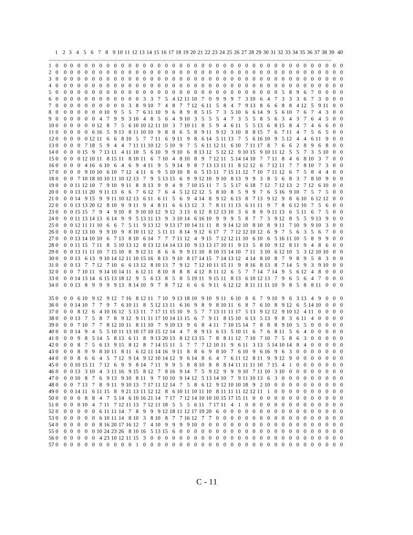
C - 11
1 2 3 4 5 6 7 8 9 10 11 12 13 14 15 16 17 18 19 20 21 22 23 24 25 26 27 28 29 30 31 32 33 34 35 36 37 38 39 40..........................................................................................................................................................................................................................1 0 0 0 0 0 0 0 0 0 0 0 0 0 0 0 0 0 0 0 0 0 0 0 0 0 0 0 0 0 0 0 0 0 0 0 0 0 0 0 02 0 0 0 0 0 0 0 0 0 0 0 0 0 0 0 0 0 0 0 0 0 0 0 0 0 0 0 0 0 0 0 0 0 0 0 0 0 0 0 03 0 0 0 0 0 0 0 0 0 0 0 0 0 0 0 0 0 0 0 0 0 0 0 0 0 0 0 0 0 0 0 0 0 0 0 0 0 0 0 04 0 0 0 0 0 0 0 0 0 0 0 0 0 0 0 0 0 0 0 0 0 0 0 0 0 0 0 0 0 0 0 0 0 0 0 0 0 0 0 05 0 0 0 0 0 0 0 0 0 0 0 0 0 0 0 0 0 0 0 0 0 0 0 0 0 0 0 0 0 0 0 5 8 9 6 7 0 0 0 06 0 0 0 0 0 0 0 0 0 0 0 0 3 3 7 5 4 12 11 10 7 0 9 9 9 7 3 10 6 4 7 3 3 3 6 7 3 0 0 07 0 0 0 0 0 0 0 0 0 0 3 8 9 10 7 4 8 7 7 12 6 11 5 8 4 7 9 13 8 6 6 8 8 4 12 5 9 11 0 08 0 0 0 0 0 0 0 10 9 5 5 7 6 11 10 9 6 8 9 8 5 15 7 3 5 10 6 6 14 9 5 6 10 7 6 7 4 3 0 09 0 0 0 0 0 0 4 7 9 9 3 10 4 8 5 6 4 9 10 3 5 5 5 4 7 3 5 5 8 5 6 3 4 3 7 6 4 5 0 010 0 0 0 0 0 0 12 8 7 5 6 10 10 12 11 10 3 7 10 11 8 5 9 4 6 11 5 5 13 6 8 15 8 4 7 4 6 6 0 011 0 0 0 0 0 6 16 5 9 13 8 11 10 10 9 8 8 6 5 8 9 11 9 12 3 10 8 8 15 7 6 7 11 4 7 5 6 5 0 012 0 0 0 0 0 12 11 6 6 8 10 5 7 7 11 6 9 11 9 8 6 14 5 11 13 7 5 6 16 10 9 5 12 4 4 6 11 9 0 013 0 0 0 0 7 18 5 9 4 4 7 11 11 10 12 5 10 9 7 5 6 11 12 11 6 10 7 11 17 8 7 6 6 2 8 9 6 8 0 014 0 0 0 0 15 9 7 13 11 4 11 10 5 6 10 9 9 10 6 8 13 12 5 12 12 9 10 15 9 10 11 12 5 5 7 3 5 10 0 015 0 0 0 0 12 10 11 8 15 11 8 10 11 6 7 10 4 8 10 8 9 7 12 11 5 14 14 10 7 7 11 8 4 6 8 10 3 7 0 016 0 0 0 0 4 16 6 10 6 4 6 9 4 11 9 5 9 14 9 8 7 13 13 11 11 8 12 12 6 7 12 11 7 7 8 10 7 3 0 017 0 0 0 0 9 10 10 6 10 7 12 4 11 6 9 5 10 10 8 6 5 15 11 7 15 11 12 7 10 7 11 12 6 7 5 8 4 4 0 018 0 0 0 7 10 18 10 10 11 10 12 13 7 9 5 13 15 6 9 9 12 10 9 10 8 13 9 9 3 8 5 6 8 3 7 8 10 9 0 019 0 0 0 11 12 10 7 9 10 9 11 8 8 13 9 9 4 9 7 10 15 11 7 5 5 17 6 18 7 12 7 12 13 2 7 12 6 10 0 020 0 0 0 13 11 20 9 11 13 6 6 7 6 12 7 6 4 5 12 12 12 5 8 10 8 5 9 9 7 6 5 16 9 10 7 5 7 5 0 021 0 0 0 14 9 15 9 9 11 10 12 13 6 11 6 11 5 6 9 4 14 8 9 12 6 13 8 7 13 9 12 9 8 6 10 6 12 12 0 022 0 0 0 13 13 20 12 8 10 9 9 11 9 4 8 11 6 6 13 12 3 7 8 11 11 13 6 11 11 9 7 8 6 12 10 7 5 6 0 023 0 0 0 15 15 7 9 4 9 10 8 9 10 10 12 9 12 3 13 6 12 8 12 13 10 3 6 8 9 9 11 13 6 5 11 6 7 5 0 024 0 0 0 11 13 14 13 6 14 9 9 5 13 11 13 9 3 10 14 6 16 10 9 9 9 5 8 7 7 3 9 12 8 5 5 9 13 9 0 025 0 0 0 12 11 11 10 6 6 7 5 11 9 13 12 9 13 17 10 14 11 11 8 9 14 12 10 8 10 8 9 11 7 10 9 9 10 3 0 026 0 0 0 12 13 10 9 9 10 9 8 10 11 12 5 11 11 8 14 9 12 6 17 7 7 12 12 10 12 6 9 7 5 6 3 5 6 7 0 027 0 0 0 13 14 10 10 6 7 13 8 10 6 14 7 7 7 11 12 4 9 15 7 12 12 11 10 6 10 6 5 16 11 10 5 8 9 9 0 028 0 0 0 11 15 7 11 8 5 10 13 12 8 13 12 14 14 13 10 9 13 13 17 10 11 9 13 5 8 10 9 12 8 11 9 4 8 6 0 029 0 0 0 13 11 11 10 7 15 10 8 9 12 11 8 6 6 9 9 11 10 8 10 15 14 10 7 11 3 10 6 12 10 5 3 12 10 10 0 030 0 0 0 13 6 13 9 10 14 12 11 10 15 16 8 13 9 10 8 17 14 15 7 14 13 12 4 14 8 10 8 7 9 8 9 5 8 3 0 031 0 0 0 13 7 7 12 7 10 6 6 13 12 8 10 13 7 9 12 7 12 10 11 15 11 9 8 16 8 13 8 7 14 5 9 3 9 10 0 032 0 0 0 7 10 11 9 14 10 14 11 6 12 11 8 10 8 8 8 4 12 8 11 12 6 5 7 7 14 7 14 9 5 6 12 4 8 0 0 033 0 0 0 14 13 14 6 15 13 18 12 9 5 6 13 8 5 8 5 19 11 9 15 11 8 13 6 10 12 13 7 9 6 5 6 4 7 0 0 034 0 0 0 13 8 9 9 9 9 13 8 14 10 9 7 8 7 12 6 6 6 9 11 6 12 12 8 11 11 11 10 9 8 5 8 8 11 0 0 0
35 0 0 0 6 10 9 12 9 12 7 16 8 12 11 7 10 9 13 18 10 9 10 9 11 6 10 8 6 7 9 10 9 6 3 13 4 9 0 0 036 0 0 0 14 10 7 7 9 7 6 10 11 8 5 12 13 11 6 16 9 8 9 8 10 11 6 8 7 6 10 8 9 12 6 5 14 10 0 0 037 0 0 0 8 12 6 4 10 16 12 5 13 11 7 17 11 15 10 9 5 7 7 13 11 11 17 5 13 9 12 12 9 10 12 4 11 0 0 0 038 0 0 0 13 7 5 8 7 8 9 12 9 11 11 17 10 14 13 15 6 7 9 11 8 15 10 6 13 5 13 9 8 3 6 11 4 0 0 0 039 0 0 0 7 10 7 7 8 12 10 11 8 11 10 7 9 10 13 9 6 8 4 11 7 10 15 14 7 8 8 8 9 10 5 5 0 0 0 0 040 0 0 0 14 9 4 5 5 10 11 13 10 17 10 15 12 14 4 7 8 9 13 6 13 5 10 11 6 7 6 8 11 5 6 4 0 0 0 0 041 0 0 0 9 8 5 14 5 8 13 6 11 8 9 13 20 13 8 12 13 15 7 8 8 11 12 7 10 7 10 7 5 8 6 3 0 0 0 0 042 0 0 0 8 7 5 6 13 9 15 8 12 8 7 14 15 11 5 7 7 7 12 10 11 9 6 11 3 13 5 14 10 14 8 4 0 0 0 0 043 0 0 0 8 9 9 8 10 11 8 11 6 12 11 14 16 9 11 8 8 6 9 8 10 7 6 10 9 6 16 9 6 3 0 0 0 0 0 0 044 0 0 0 8 6 6 4 5 7 12 9 14 9 12 10 14 12 9 6 14 8 6 4 7 6 11 12 8 11 9 9 12 9 0 0 0 0 0 0 045 0 0 0 10 15 11 7 12 6 9 9 8 14 7 11 9 9 5 8 8 10 8 8 8 14 11 11 11 10 7 15 4 1 0 0 0 0 0 0 046 0 0 0 13 3 10 4 3 11 16 9 15 8 12 7 8 16 9 14 7 5 9 12 9 9 9 10 7 11 10 3 10 0 0 0 0 0 0 0 047 0 0 0 10 8 7 6 9 13 9 10 8 11 9 7 10 10 9 14 12 5 13 14 10 7 9 11 10 13 6 3 0 0 0 0 0 0 0 0 048 0 0 0 7 13 7 8 9 11 9 10 13 7 17 11 12 14 7 5 8 6 12 9 12 10 10 18 9 2 10 0 0 0 0 0 0 0 0 0 049 0 0 0 14 11 6 11 15 8 9 21 13 11 12 12 8 6 10 11 10 11 10 8 11 11 11 12 12 11 1 0 0 0 0 0 0 0 0 0 050 0 0 0 0 8 8 4 7 5 14 6 10 16 21 14 7 17 7 12 14 10 10 10 15 17 15 11 0 0 0 0 0 0 0 0 0 0 0 0 051 0 0 0 0 10 4 7 11 7 12 11 13 7 12 11 18 5 5 5 6 11 7 17 11 4 1 0 0 0 0 0 0 0 0 0 0 0 0 0 052 0 0 0 0 0 0 6 11 11 14 7 8 9 9 9 12 18 11 12 17 19 20 6 0 0 0 0 0 0 0 0 0 0 0 0 0 0 0 0 053 0 0 0 0 0 0 6 10 11 14 8 10 3 8 10 8 7 7 16 12 7 7 0 0 0 0 0 0 0 0 0 0 0 0 0 0 0 0 0 054 0 0 0 0 0 0 8 16 20 17 16 12 7 4 10 9 9 9 9 10 0 0 0 0 0 0 0 0 0 0 0 0 0 0 0 0 0 0 0 055 0 0 0 0 0 0 10 24 23 26 8 10 16 5 13 15 6 0 0 0 0 0 0 0 0 0 0 0 0 0 0 0 0 0 0 0 0 0 0 056 0 0 0 0 0 0 4 23 10 12 11 15 3 0 0 0 0 0 0 0 0 0 0 0 0 0 0 0 0 0 0 0 0 0 0 0 0 0 0 057 0 0 0 0 0 0 0 0 0 0 0 1 0 0 0 0 0 0 0 0 0 0 0 0 0 0 0 0 0 0 0 0 0 0 0 0 0 0 0 0
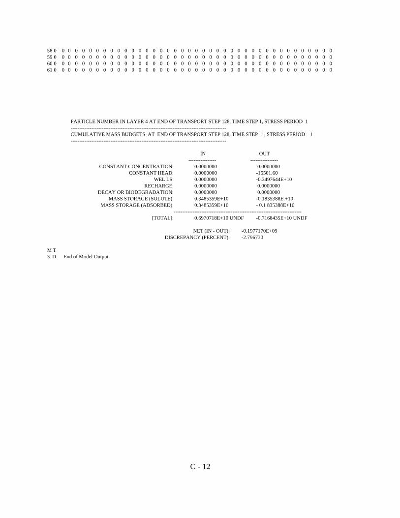
C - 12
58 0 0 0 0 0 0 0 0 0 0 0 0 0 0 0 0 0 0 0 0 0 0 0 0 0 0 0 0 0 0 0 0 0 0 0 0 0 0 0 059 0 0 0 0 0 0 0 0 0 0 0 0 0 0 0 0 0 0 0 0 0 0 0 0 0 0 0 0 0 0 0 0 0 0 0 0 0 0 0 060 0 0 0 0 0 0 0 0 0 0 0 0 0 0 0 0 0 0 0 0 0 0 0 0 0 0 0 0 0 0 0 0 0 0 0 0 0 0 0 061 0 0 0 0 0 0 0 0 0 0 0 0 0 0 0 0 0 0 0 0 0 0 0 0 0 0 0 0 0 0 0 0 0 0 0 0 0 0 0 0
PARTICLE NUMBER IN LAYER 4 AT END OF TRANSPORT STEP 128, TIME STEP 1, STRESS PERIOD 1------------------------------------------------------------------------------------------CUMULATIVE MASS BUDGETS AT END OF TRANSPORT STEP 128, TIME STEP 1, STRESS PERIOD 1------------------------------------------------------------------------------------------
IN OUT---------------- ----------------
CONSTANT CONCENTRATION: 0.0000000 0.0000000CONSTANT HEAD: 0.0000000 -15501.60
WEL LS: 0.0000000 -0.3497644E+10RECHARGE: 0.0000000 0.0000000
DECAY OR BIODEGRADATION: 0.0000000 0.0000000MASS STORAGE (SOLUTE): 0.3485359E+10 -0.1835388E.+10
MASS STORAGE (ADSORBED): 0.3485359E+10 - 0.1 835388E+10--------------------------------------------------------------------------
[TOTAL]: 0.6970718E+10 UNDF -0.7168435E+10 UNDF
NET (IN - OUT): -0.1977170E+09DISCREPANCY (PERCENT): -2.796730
M T3 D End of Model Output

Appendix D
POST-PROCESSING PROGRAMS
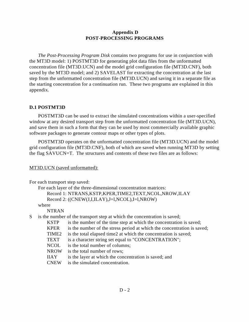
D - 2
Appendix DPOST-PROCESSING PROGRAMS
The Post-Processing Program Disk contains two programs for use in conjunction withthe MT3D model: 1) POSTMT3D for generating plot data files from the unformattedconcentration file (MT3D.UCN) and the model grid configuration file (MT3D.CNF), bothsaved by the MT3D model; and 2) SAVELAST for extracting the concentration at the laststep from the unformatted concentration file (MT3D.UCN) and saving it in a separate file asthe starting concentration for a continuation run. These two programs are explained in thisappendix.
D.1 POSTMT3D
POSTMT3D can be used to extract the simulated concentrations within a user-specifiedwindow at any desired transport step from the unformatted concentration file (MT3D.UCN),and save them in such a form that they can be used by most commercially available graphicsoftware packages to generate contour maps or other types of plots.
POSTMT3D operates on the unformatted concentration file (MT3D.UCN) and the modelgrid configuration file (MT3D.CNF), both of which are saved when running MT3D by settingthe flag SAVUCN=T. The structures and contents of these two files are as follows:
MT3D.UCN (saved unformatted):
For each transport step saved:For each layer of the three-dimensional concentration matrices:
Record 1: NTRANS,KSTP,KPER,TIME2,TEXT,NCOL,NROW,ILAYRecord 2: ((CNEW(J,I,ILAY),J=l,NCOL),I=l,NROW)
whereNTRAN
S is the number of the transport step at which the concentration is saved;KSTP is the number of the time step at which the concentration is saved;KPER is the number of the stress period at which the concentration is saved; TIME2 is the total elapsed time2 at which the concentration is saved;TEXT is a character string set equal to "CONCENTRATION";NCOL is the total number of columns;NROW is the total number of rows;IIAY is the layer at which the concentration is saved; and CNEW is the simulated concentration.

D - 3
MT3D.CNF (saved in free format):
Record 1: NLAY, NROW, NLAYRecord 2: (DELR(J), J=l,NCOL)Record 3: (DELC(l),I=l,NROW)Record 4: ((HTOP(J,I), J=l,NCOL),I=l,NROW)Record 5: (((DZ(J,I,K), J=l,NCOL),I=l,NROW),K=l,NLAY)Record 6: CINACT
whereNLAY is the total number of layers;DELR is the cell width along the row direction;DELC is the cell width along the column direction;HTOP is the top elevation of the first model layer,DZ is the thickness of each cell in the grid; andCINACT is the value used in the model for indicating inactive concentration cells.
POSTMT3D is an interactive program. To run it, simply type the name of its executable file.The program will prompt the user for the various input items. The user can select theconcentration at the desired step by specifying either the number of the transport step, time stepand stress period, or the total elapsed time, which ever is more convenient. The user can alsodefine a "window" within which the graphic data files are desired by specifying the cell indices(column, row and layer) at the upper left and lower right corners of the window. For example,to generate a data file for a cross sectional contour map along the 5th column, from row 20 to row40 and from layer 1 to 10, enter the (J,I,K) indices at the upper left comer as 5,20, 1, and at thelower right corner as 5,40,10. Similarly, to generate a data file for a cross sectional contour mapalong the 5th row, from column 20 to column 40 and from layer 1 to 10, enter the (J,I,K) indicesat the upper left corner as 20,5,1, and at the lower right corner as 40, 5,10. Moreover, to generatea data file for a contour map on the 5th layer, from column 20 to column 40 and from row 1 torow 10, enter the (J,I,K) indices at the upper left corner as 20,1,5 and at the lower right corner as40,10,5. Finally, to generate a data file for a contour map on the water table, i.e., the cells in theuppermost active layers instead of a specific layer, from column 20 to column 40 and from row1 to row 10, enter the (J,I,K) indices at the upper left corner as 20,1,0 and at the lower rightcorner as 40, 10,0.
For output, POSTMT3D can write data files in two formats, referred to as the "TOPO"format and the "GRID" format, according to the convention used by Golden Software'sSURFER® graphic package. The TOPO format as listed below writes the concentration withina user-defined window of regular model mesh spacing to an output file, directly useable forgenerating contour maps by a contouring program such as the TOPO program included inSURFER®. The GRID format as listed below writes the concentration at each node with thenodal coordinates within the user-defmed window to the output file. This format is useful forgenerating data files of irregular model mesh spacing to be used by a gridding program such as
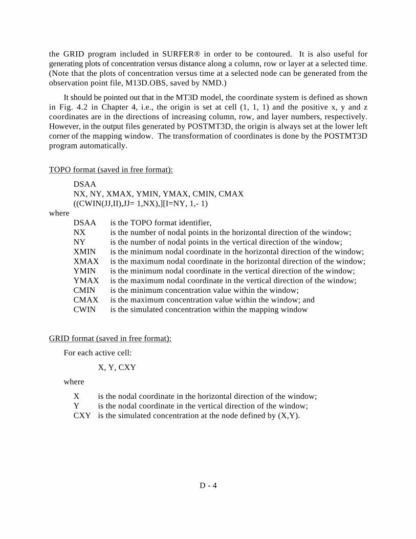
D - 4
the GRID program included in SURFER® in order to be contoured. It is also useful forgenerating plots of concentration versus distance along a column, row or layer at a selected time.(Note that the plots of concentration versus time at a selected node can be generated from theobservation point file, M13D.OBS, saved by NMD.)
It should be pointed out that in the MT3D model, the coordinate system is defined as shownin Fig. 4.2 in Chapter 4, i.e., the origin is set at cell (1, 1, 1) and the positive x, y and zcoordinates are in the directions of increasing column, row, and layer numbers, respectively.However, in the output files generated by POSTMT3D, the origin is always set at the lower leftcorner of the mapping window. The transformation of coordinates is done by the POSTMT3Dprogram automatically.
TOPO format (saved in free format):
DSAANX, NY, XMAX, YMIN, YMAX, CMIN, CMAX ((CWIN(JJ,II),JJ= 1,NX),][I=NY, 1,- 1)
whereDSAA is the TOPO format identifier,NX is the number of nodal points in the horizontal direction of the window;NY is the number of nodal points in the vertical direction of the window;XMIN is the minimum nodal coordinate in the horizontal direction of the window;XMAX is the maximum nodal coordinate in the horizontal direction of the window;YMIN is the minimum nodal coordinate in the vertical direction of the window;YMAX is the maximum nodal coordinate in the vertical direction of the window;CMIN is the minimum concentration value within the window;CMAX is the maximum concentration value within the window; andCWIN is the simulated concentration within the mapping window
GRID format (saved in free format):
For each active cell:
X, Y, CXY
where
X is the nodal coordinate in the horizontal direction of the window;Y is the nodal coordinate in the vertical direction of the window;CXY is the simulated concentration at the node defined by (X,Y).
D - 5
D.2 SAVELAST
If a continuation run as described in Section 6.10 is desired, the concentration from the finalstep of the preceding run can be used as the starting concentration for the continuation run. Theconcentration is saved in the default unformatted concentration ffle, MT3D.UCN, which isdirectly readable by the array reader RARRAY. If there is more than one step of concentrationsaved in MT3D.UCN, then SAVEIAST can be used to extract the concentration at the final stepand put it in a separate unformatted file . To run it, simply type the SAVELAST executable filename and enter the names of input and output files.
Appendix E
ABBREVIATED INPUT INSTRUCTIONS

E - 2
BASIC TRANSPORT PACKAGE
ID VARIABLE NAME FORMAT EXPLANATION
Al HEADING(1) A80 First line of title for simulation runA2 HEADING(2) A80 Second line of the titleA3 NLAY, NROW,NCOL,NPER 4I10 Number of layers, rows, columns
and stress periodsA4 TUNIT, LUNIT, MUNIT 3A4 Unit names for time, length, and
massA5 TRNOP(10) 10L2 Transport options (ADV, DSP,
SSM, RCT)A6 LAYCON(NLAY) 40I2 Model layer type codeA7 DELR(NCOL) RARRAY Cell width along rows (or x-axis)A8 DELC (NROW) RARRAY Cell width along columns (or y-
axis)A9 HTOP (NCOL, NROW) RARRAY Top elevation of the first model
layerA10 DZ (NCOL, NROW) (One array for each layer) RARRAY Cell thicknessA11 PRSITY (NCOL, NROW) (One array for each layer) RARRAY PorosityA12 ICBUND (NCOL, NROW) (One array for each layer) IARRAY Concentration boundary indicator
arrayA13 SCONC (NCOL, NROW) (One array for each layer) RARRAY Starting concentrationsA14 CINACT F10.0 Value indicating inactive
concentration cellsA15 IFMTCN,IFMTNP,IFMTRF,IFMTDP,SAVUCN 4I10, L10 Output control optionsA16 NPRS I10 Interval for printing or saving
simulation results(Enter A17 if NPRS > 0)A17 TIMPRS (NPRS) 8F10.0 Total elapsed times at which
simulation results should be printedor saved
A18 NOBS I10 Number of observation points(Enter A19 NOBS times if NOBS > 0)A19 KOBS, IOBS, JOBS 3I10 Location of observation points
(layer, row, column)A20 CHKMAS L10 Flag for saving mass balance
summary file(Repeat A21 through A23 for each stress period)A21 PERLEN, NSTP, TSMULT F10.0, I10, F10.0 Length of stress period, number of
time steps, time step multiplier(Enter A22 if TSMULT < or = 0)A22 TSLNGH (NSTP) 8F10.0 Length of time steps if geometric
progression of time steps is not usedin flow model
A23 DTO, MXSTRN F10.0, I10 Transport stepsize, maximumtransport steps allowed in one timestep

E - 3
ADVECTION PACKAGE
ID VARIABLE NAME FORMAT EXPLANATION
B1 MIXELM, PERCEL, MXPART I10, F10.0, I10 Advection solution flag; number of cells that anyparticle is allowed to move in one transport step;maximum number of moving particles allowedMIXELM = 1, MOC
= 2, MMOC= 3, HMOC= 0, Finite difference
(Enter B2 if MIXELM = 1, 2 or 3)B2 ITRACK, WD I10, F10 Particle tracking option, concentration weighting
factor(Enter B3 if MIXELM=1 or 3)B3 DCEPS,NPLANE,NPL,NPH,NPMIN,
NPMAX,SRMULT F10.0, 5I10, F10.0 Particle distribution control parameters for theMOC scheme
(Enter B4 of MIXELM=2, or 3)B4 INTERP, NLSINK, NPSINK 3I10 Solution flags for the MMOC scheme(Enter B5 if MIXELM=3)B5 DCHMOC F10.0 Critical cell concentration gradient for controlling
the selective use of the MOC or MMOC scheme:MOC is used if DCCELL > DCHMOC;MMOC is used if DCCELL < or = DCHMOC
DISPERSION PACKAGE
ID VARIABLE NAME FORMAT EXPLANATION
C1 AL (NCOL, NROW) (One array for each layer) RARRAY Longitudinal dispersivityC2 TRPT (NLAY) RARRAY Ratio of horizontal transverse
dispersivity to longitudinal dispersivityC3 TRPV (NLAY) RARRAY Ratio of vertical transverse dispersivity
to longitudinal dispersivityC4 DMCOEF (NLAY) RARRAY Effective molecular diffusion
coefficient

E - 4
SINK & SOURCE MIXING PACKAGE
ID VARIABLE NAME FORMAT EXPLANATION
D1 FWEL, FDRN, FRCH, FEVT, FRIV, FGHB 6L2 Flags for well, drain, recharge, evapotranspiration,river,general-head-dependent boundary, respectively
D2 MXSS I10 Maximum number of all point sources and sinksin the flow model
(Repeat D3 through D8 for each stress period)(Enter D3 if FRCH=T)D3 INCRCH I10 Flag indicating whether concentration of recharge
flux should be read(Enter D4 if FRCH=T and INCRCH > or = 0)D4 CRCH (NCOL, NROW) RARRAY Concentration of recharge flux(Enter D5 if FEVT = T)D5 INCEVT I10 Flag indicating whether concentration of
evapotranspiration fluxes should be read(Enter D6 if FEVT = T and INCEVT > or = 0)D6 CEVT (NCOL, NROW) RARRAY Concentration of evapotranspiration fluxD7 NSS I10 Number of point sources of specified
concentrations(Enter D8 NSS times if NSS > 0)D8 KSS, ISS, JSS, CSS, ITYPE 3I10, F10.0,I10 Layer, row, column, concentration, and type of
point sources which are of specificconcentrations
ITYPE = 1, constant-head cell= 2, well= 3, drain= 4, river= 5, general-head-dependent
boundary cell

E - 5
CHEMICAL REACTION PACKAGE
ID VARIABLE NAME FORMAT EXPLANATIONEl ISOTHM, IREACT 2I10 Flags indicating type of sorption and first order rate
reactionsISOTHM =1, Linear
= 2, Freundlich= 3, Langmuir= 0, None
IREACT = 1, Decay or biodegradation= 0, None
(Enter E2, E3 and E4 if ISOTHM > 0)E2 RHOB (NLAY) RARRAY Bulk density of the porous mediuinE3 SP1 (NLAY) RARRAY First sorption constantE4 SP2 (NLAY) RARRAY Second sorption constant(Enter E5 and E6 if IREACT > 0)E5 RC1 (NLAY) RARRAY First-order rate reaction constant for the dissolved
phaseE6 RC2 (NLAY) RARRAY First-order rate reaction constant for the sorbed phase
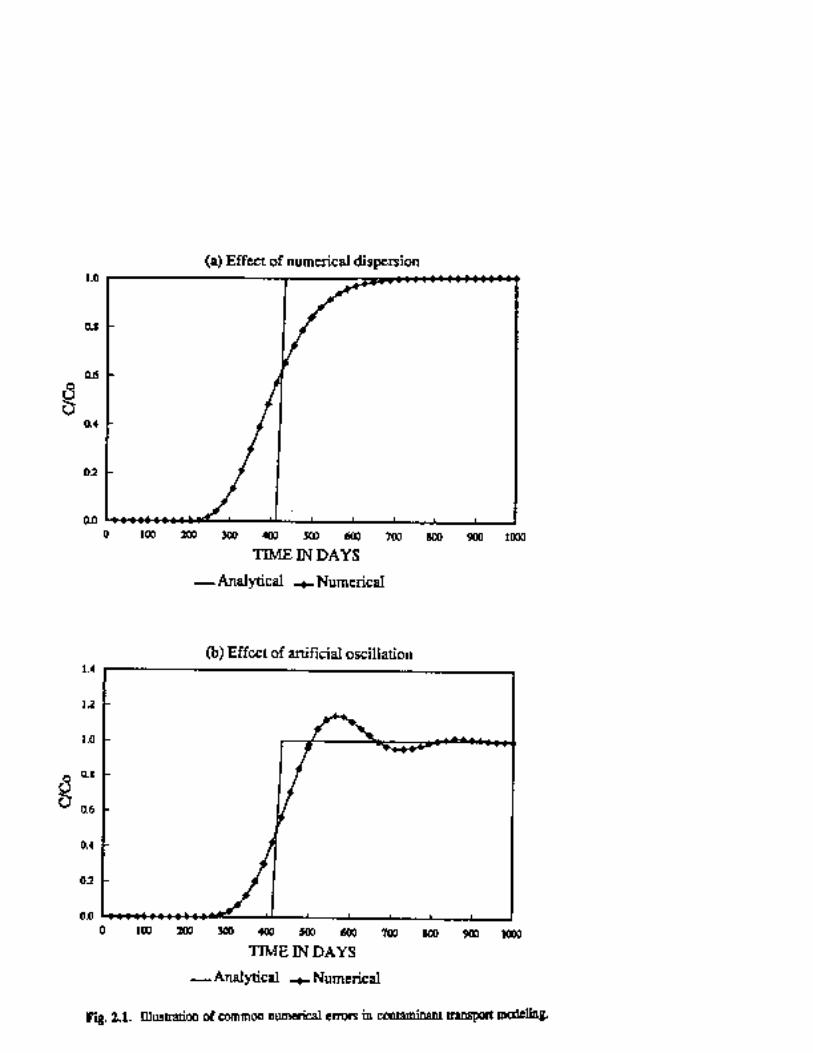
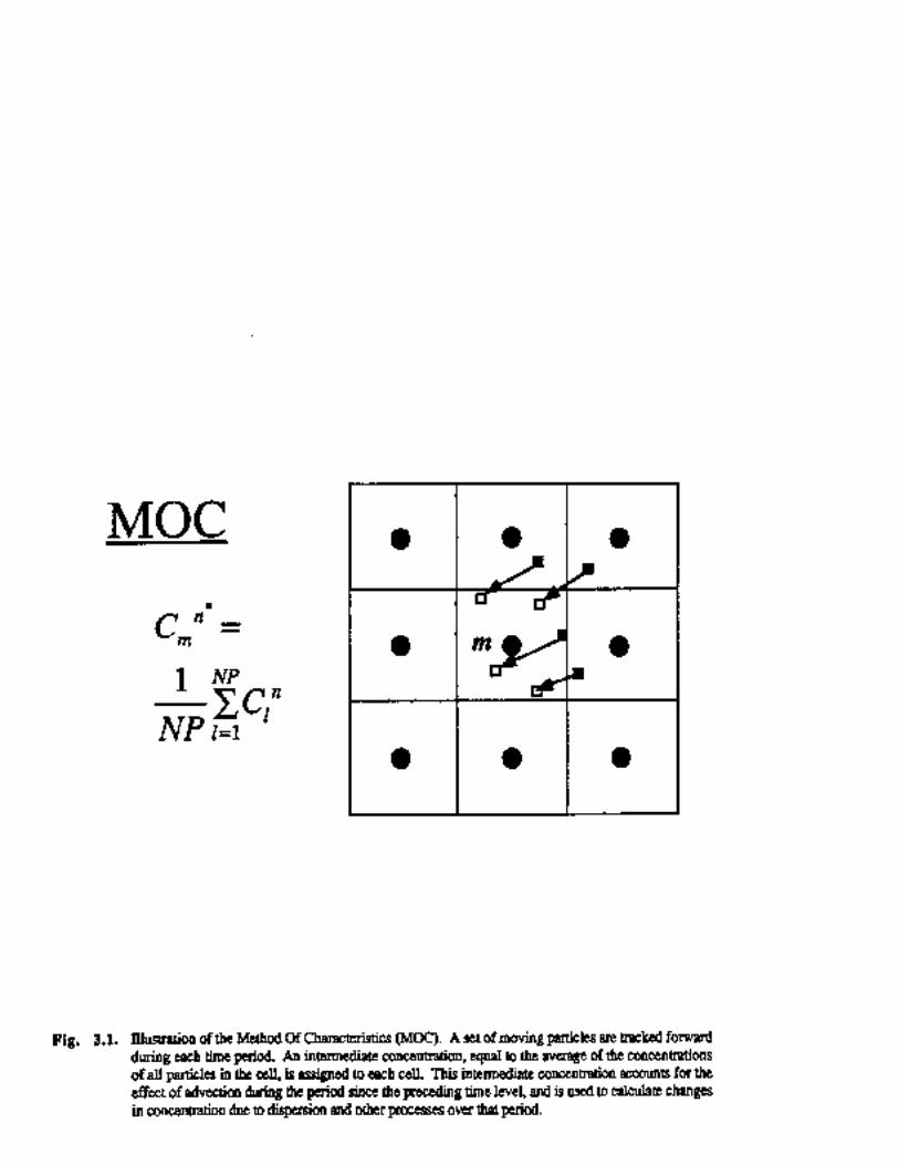

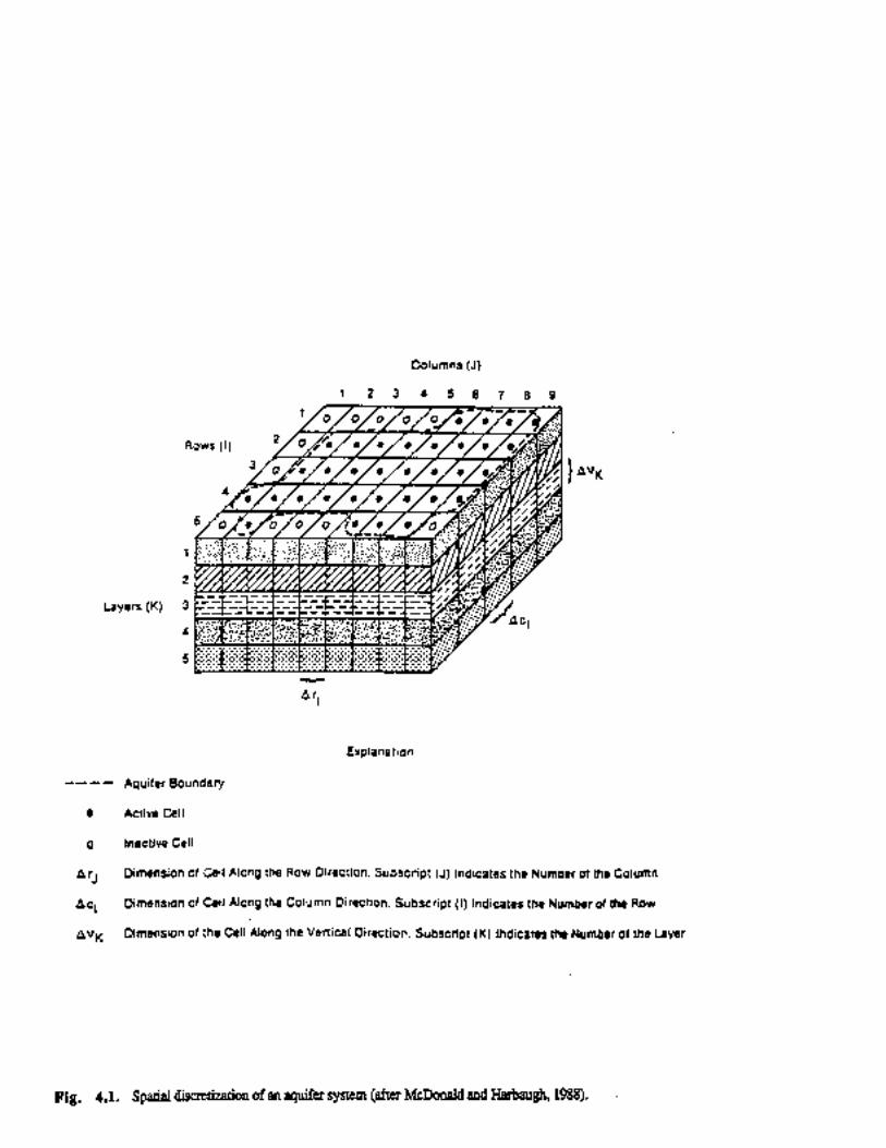

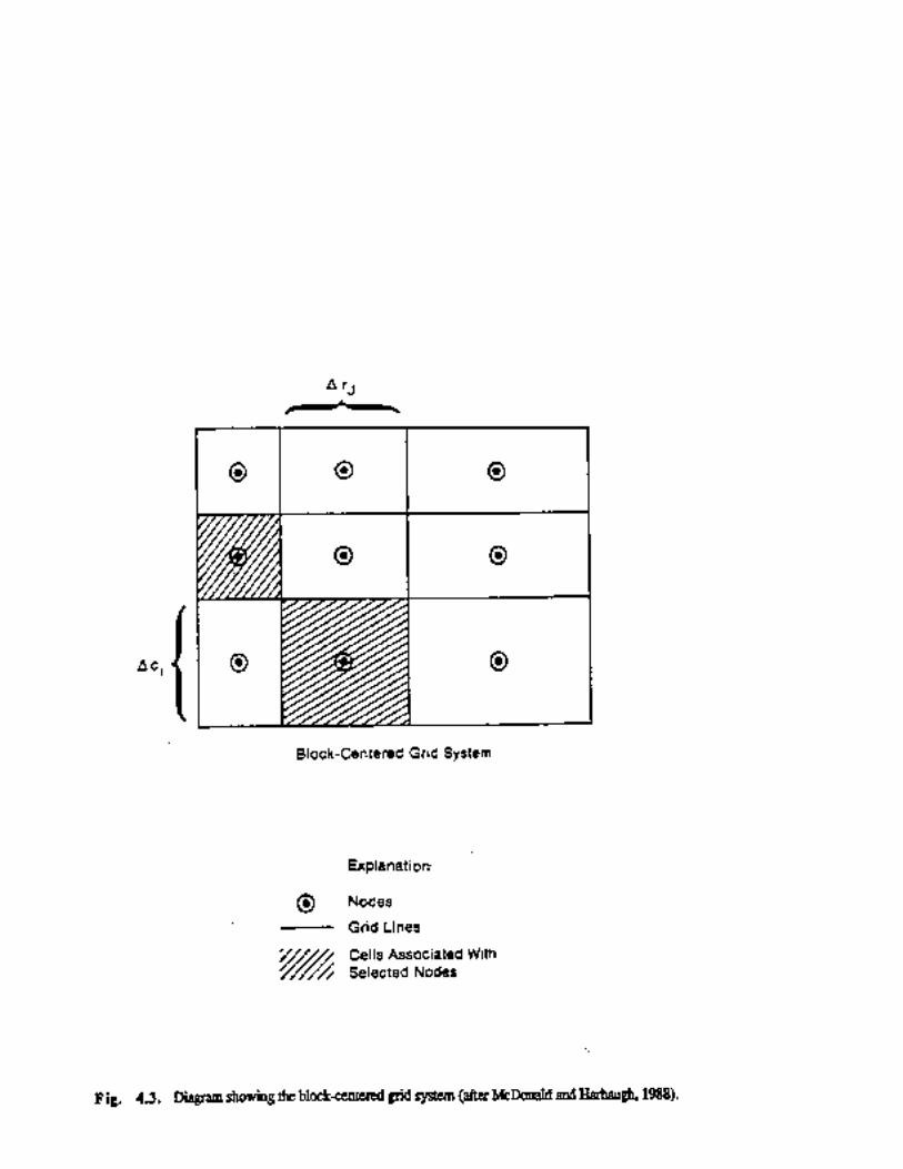


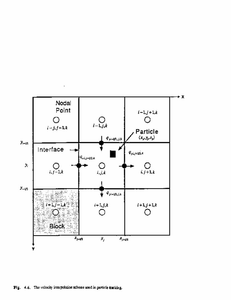

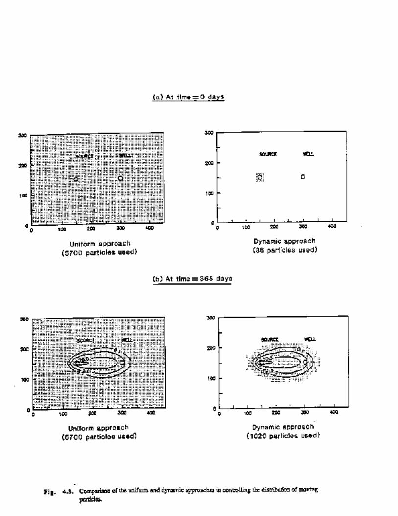
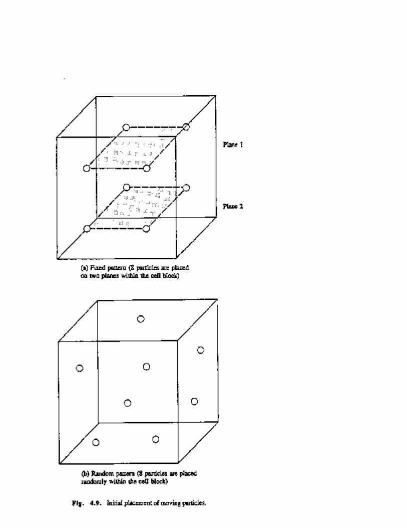

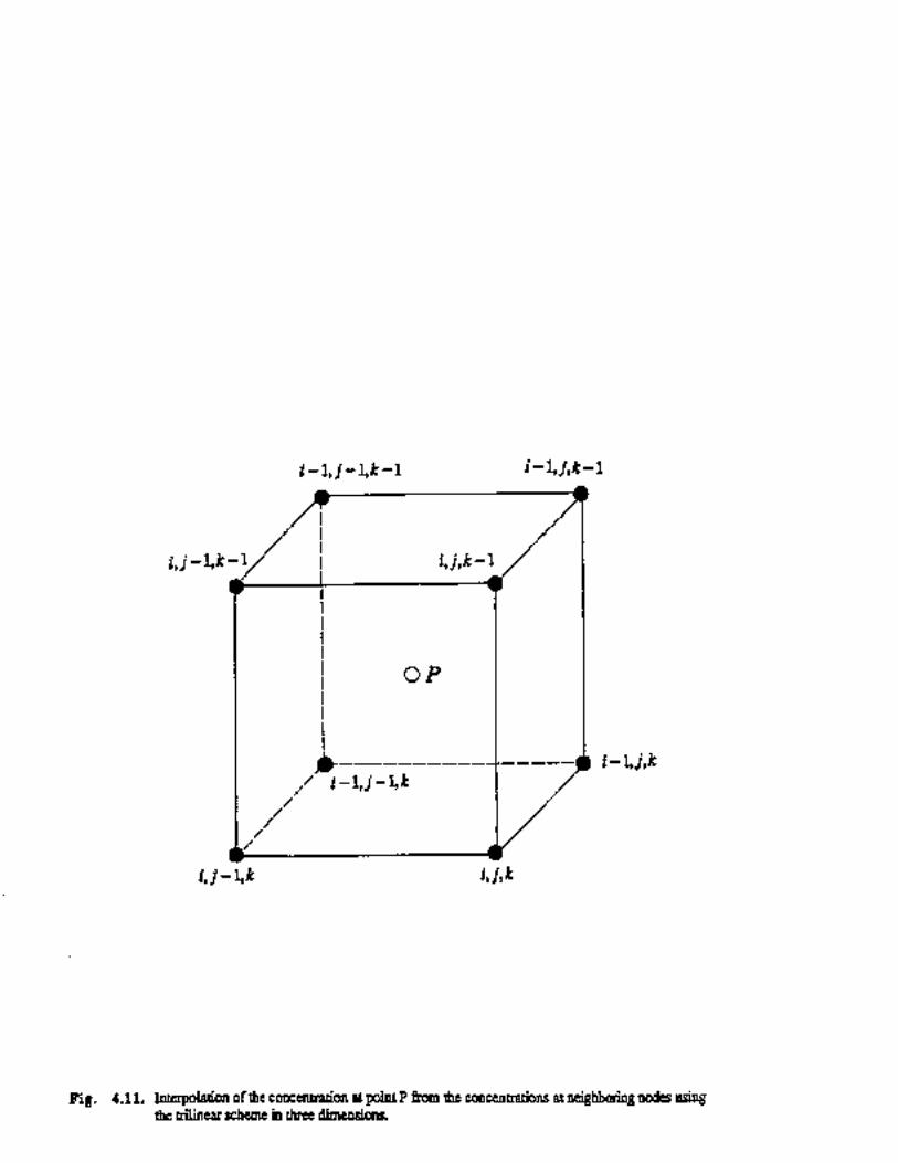
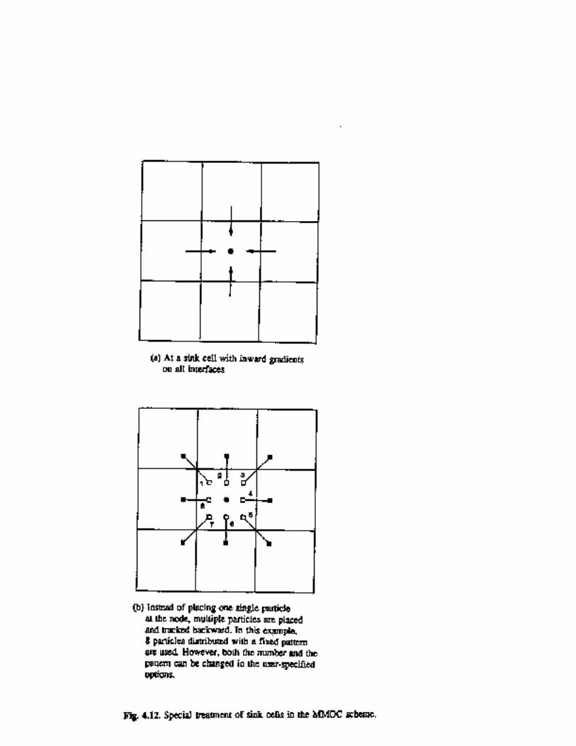


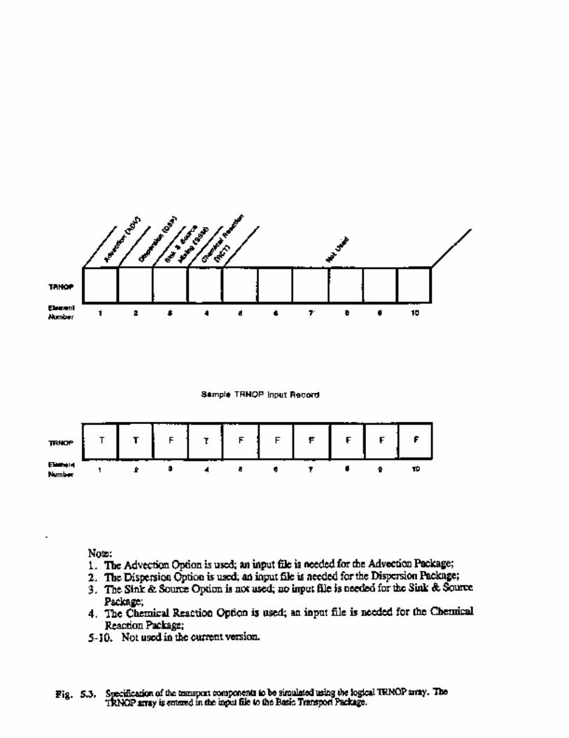
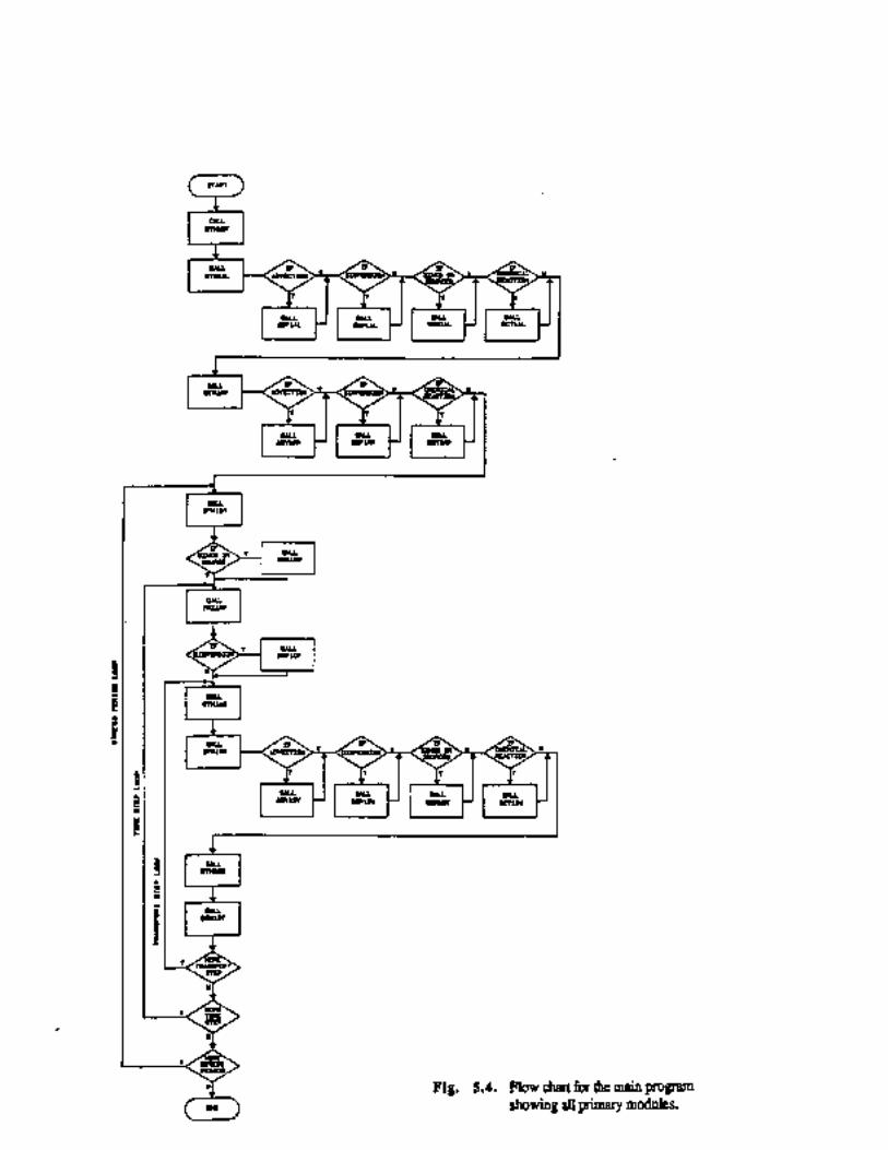


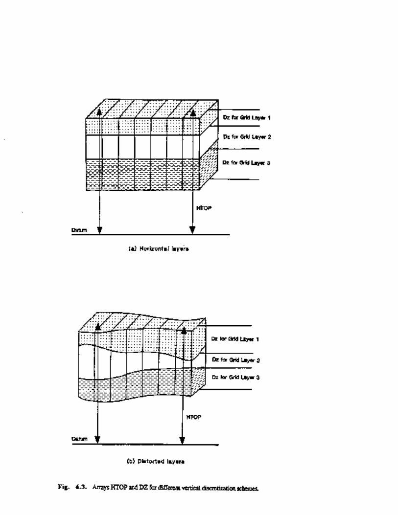


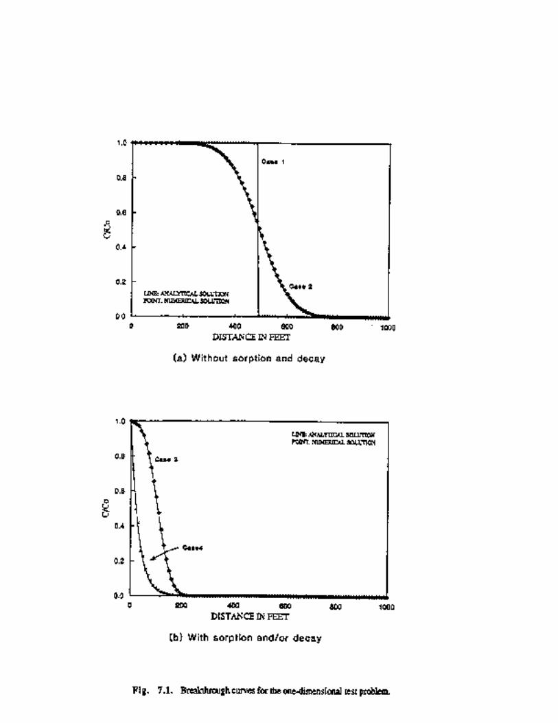
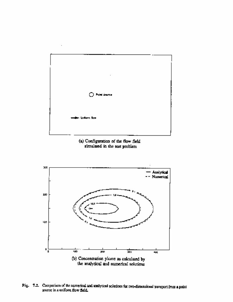

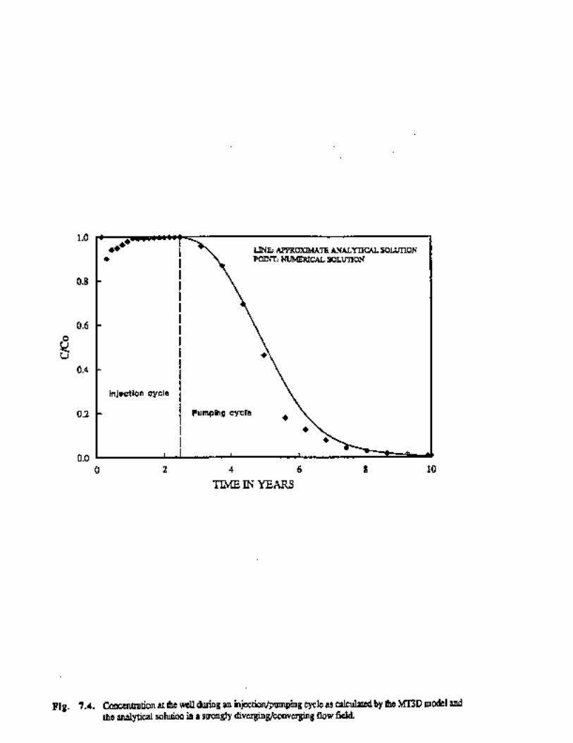
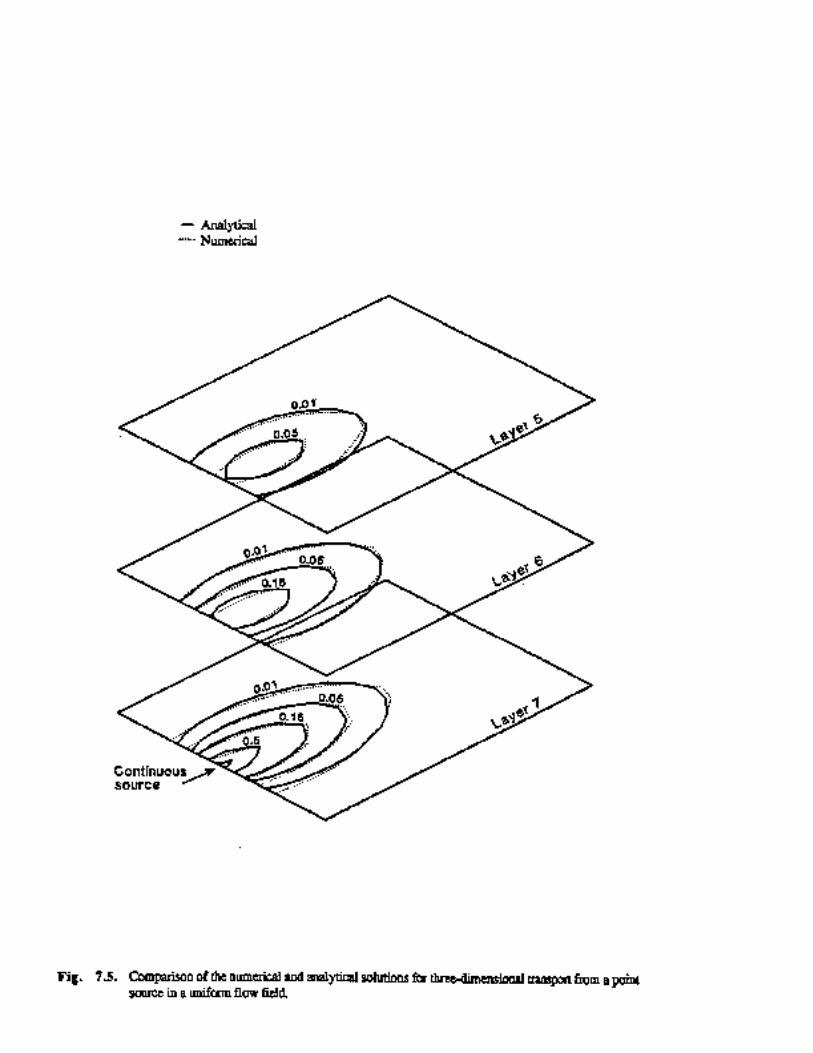


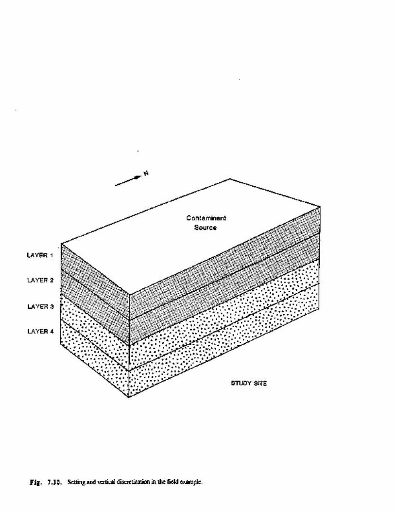


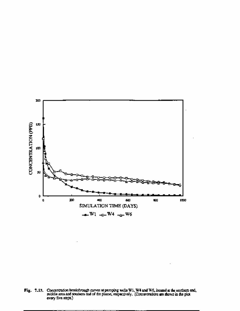


![3D Texture-Based Flow Visualization...[Weiskopf & Ertl 04] D. Weiskopf, T. Ertl. GPU-based 3D texture advection for the visualization of unsteady flow fields. In Proceedings of WSCG](https://static.fdocuments.us/doc/165x107/5f6973d0319edd387c3cb14e/3d-texture-based-flow-visualization-weiskopf-ertl-04-d-weiskopf-t.jpg)