M. Salahi, F. Mehrdoust, F. Piri

University of Guilan, Rasht, Iran

CVaR Robust Mean-CVaR Portfolio Optimization

Abstract:

One of the most important problems faced by every investor is asset allocation. An investor during

making investment decisions has to search for equilibrium between risk and returns. Risk ‎and ‎return are

uncertain parameters in ‎the ‎suggested portfolio optimization models and should be estimated to solve

the‎‎problem. The estimation might‎ lead ‎to ‎large ‎error in the final decision. One of the widely used and

effective approaches for optimization with data uncertainty is robust optimization. In this paper, we

present a new robust portfolio optimization technique for mean-CVaR portfolio selection problem

under the estimation risk in mean return. We additionally use CVaR as risk measure, to measure the

estimation risk in mean return. Moreover, to solve the model efficiently, we use the smoothing

technique of Alexander et al. [1]. We compare the performance of the CVaR robust mean-CVaR model

with robust mean-CVaR models using interval and ellipsoidal uncertainty sets. It is observed that the CVaR robust mean-CVaR portfolios are more diversified. Moreover, we study the impact of the value

of confidence level on the conservatism level of a portfolio and also on the value of the maximum

expected return of the portfolio.

Keywords: Portfolio Optimization; Robust Optimization; Value at Risk; Conditional Value at Risk;

Smoothing

1 Introduction

Portfolio optimization is one of the best known approaches in financial portfolio selection. The earliest

technique to solve the portfolio selection problem was developed by Harry Markowitz in the 1952. In

this method that is called mean-variance (MV) portfolio optimization model, the portfolio return is

measured by the expected return of the portfolio and the associated risk is measured by the variance of

portfolio returns [16].

Variance as the risk measure has its weaknesses. Controlling the variance does not only lead to low

deviation from the expected return on the downside, but also on the upside [17]. Hence, alternative risk

measures have been suggested to replace the variance such as Value at Risk (VaR ) that manage and

control risk in terms of percentiles of loss distribution. Instead of regarding the both upside and

downside of the expected return, VaR considers only the downside of the expected return as risk and

represents the predicted maximum loss with a specified confidence level (e.g. 95%) over a certain

period of time (e.g. one day) [5, 6, 15].

VaR is a popular risk measure. However, VaR may have drawbacks and undesirable properties that limit

its

use [2, 11, 14]. Such as lack of subadditivity, i.e., VaR of two different investment portfolios may be

greater than the sum of the individual VaR s. Also, VaR is nonconvex and nonsmooth and has multiple

local minimum, while we seek the global minimum [6, 10, 14]. So alternative risk measures was

introduced such as Conditional Value at Risk ( CVaR ) - the conditional expected value of loss, under the

condition that it exceeds the value at risk [5]. VaR implies that “what is the maximum loss that we

realize?” but CVaR asks: “How do we expect to incur losses when situation is undesirable?”. Numerical

experiments show that minimum CVaR often lead to optimal solutions close to the minimum VaR ,

because VaR never exceeds CVaR [15]. CVaR has better properties than VaR . CVaR optimization is a

convex optimization problem and thus it is easy to optimize [6]. It is demonstrated that linear

programming techniques can be used for optimization of CVaR risk measure [10, 15].

The rest of the paper is arranged as follows. In Section 2, we state the mean- CVaR portfolio selection

problem. Then because of the inevitable estimation error of the mean return of the assets, we present

robust optimization by CVaR in Section 3. To solve the model efficiently, we use the smoothing

technique of Alexander et al. [1]. Finally, in Section 4, we compare the performance of the CVaR

robust mean-CVaR model with robust mean-CVaR models using interval and ellipsoidal uncertainty

sets on an example. We have observed that the CVaR robust mean-CVaR portfolios are more

diversified and they are sensitive to initial data used to generate each set of samples. Moreover, we

demonstrate the value of confidence level affects on the conservatism level, diversification and also on

the value of the maximum expected return of the resulting portfolios.

2 Mean-Conditional Value at Risk

Consider assets 1, ..., nS S, 2n , with random returns. Suppose i denote the expected return of asset iS

and also consider ix as the proportion of holding in the ith asset. We can represent the expected return

of the resulting portfolio x as follows:

1 1[ ] ... . (1)T

n nE x x x x

Also, we will assume that the set of feasible portfolios is a nonempty polyhedral set and represent that

as | , x Ax b Cx d where A is a m n matrix, b is an m -dimensional vector, C is a p n

matrix and d is a p -dimensional vector [6]. In particular, one of the constraints in the set is

1

1 = n

i

i

x

.

Let ( , )f x y denote the loss function when we choose the portfolio x from a set of feasible portfolios

and y is the realization of the random events (the vector of the asset returns of n assets). We consider

the portfolio return loss, ( , )f x y , the negative of the portfolio return that is a convex (linear) function of

the portfolio variables x :

1 1( , ) [ ... ]. (2)T

n nf x y y x y x y x

We assume that the random vector y has a probability density function denoted by ( )p y . For a fixed

decision vector x , the cumulative distribution function of the loss associated with that vector is

computed as follows:

( , )( , ) ( ) . (3)

f x yx p y dy

Then, for a given confidence level , the VaR associated with portfolio x is represented as

( ) min | , . (4)VaR x x

Also, we define the CVaR associated with portfolio x as:

( , ) ( )

1( ) ( , ) ( ) . (5)

(1 ) f x y VaR xCVaR x f x y p y dy

Theorem 1-2. We always have: ( ) ( )CVaR x VaR x

, that means CVaR of a portfolio is always at least

as big as its VaR . Consequently, portfolios with small CVaR also have small VaR . However, in general

minimizing CVaR and VaR are not equivalent.

Proof: See [6].

Since the definition of CVaR implies the VaR function clearly, it is difficult to work with and optimize

this function. Instead, the following simpler auxiliary function is considered:

( , )

1( , ) ( ( , ) ) ( ) , (6)

(1 )

f x yF x f x y p y dy

and or

1( , ) ( ( , ) ) ( ) , (7)

(1 ) F x f x y p y dy

where max , 0a a

. This function, considered as a function of , has the following important

properties that makes it useful for the computation of VaR and CVaR [6]:

1. F is a convex function of .

2. VaR is a minimizer over of

F .

3. The minimum value over of the function F is

CVaR .

As a consequence of the listed properties, we immediately deduce that, in order to minimize ( )CVaR x

over x , we need to minimize the function ( , )F x

with respect to x and simultaneously:

,min ( ) min ( , ). (8)

x xCVaR x F x

Consequently, we can optimize CVaR directly, without needing to compute VaR first. Since we

assumed that the loss function ( , )f x y is the convex (linear) function of the portfolio variables x , so

( , )F x is also a convex (linear) function of x . In this case, provided the feasible portfolio set is

also convex, the optimization problems in equation (8) are convex optimization problems that can be

solved using well known optimization techniques for such problems.

Instead of using the density function ( )p y of the random events in formulation (7) that it is often

impossible or undesirable to compute it, we can use a number of scenarios in the names of iy for

1,...,i T . In this case, we consider the following approximation to the function( , )F x

:

1

1( , ) ( ( , ) ) . (9)

(1 )

T

i

F x f x yiT

Now, in the problemmin ( )

xCVaR x

, we replace ( , )F x

with ( , )F x

:

,1

1min ( ( , ) ) . (10)

(1 )

T

xi

f x yiT

To solve this optimization problem, we introduce artificial variables iz to replace

( ( , ) )if x y

. To do

so, we add the constraints 0iz

and ( , )i iz f x y

to the problem [15]:

, ,1

1min

(1 )

. . 0, 1, ..., (11)

( , ) , 1, ...,

.

T

ix z

i

i

i i

zT

s t z i T

z f x y i T

x

It should be noted that risk managers often try to optimize risk measure while expected return is more

than a threshold value. In this case, we can represent mean- CVaR model as follows:

, ,1

1min

(1 )

. . , (12)

0, 1, ...,

( , ) , 1, ...,

,

T

ix z

i

T

i

i i

zT

s t x R

z i T

z f x y i T

x

or

, ,1

1min (

(1 )

. . 0, 1, ..., (13)

( , ) , 1, ...,

,

)

TT

ix z

i

i

i i

x zT

s t z i T

z f x y i T

x

where the first constraint of problem (12) indicates that the expected return is no less than the target

value R and 0 used in problem (13) is risk aversion parameter that adapts the balance between

expected return and ( )CVaR x . It is important to note that there is an equivalence between R and so

that the problems (12) and (13) generate the same efficient frontiers. Since ( , )f x y is linear in x , all the

expressions ( , )i iz f x y

represent linear constraints and therefore the problem is a linear

programming problem that can be efficiently solved using the simplex or interior point methods.

3 CVaR robust mean- CVaR model

One of the uncertain parameters for mean- CVaR model is and using estimations for this parameter

leads to an estimation risk in portfolio selection. In particular, small differences in the estimations of

can create large changes in the composition of an optimal portfolio. One way to reduce the sensitivity

of mean- CVaR model to the parameter estimations is using robust optimization to determine the optimal

portfolio under the worst case scenario in the uncertainty set of the expected return. To this end, we

represented robust mean- CVaR models with interval and ellipsoidal uncertainty sets in the previous

studies that have been demonstrated in formulations (14) and (15) respectively.

, ,1

1min

(1 )

. . ( ) , (14)

0, 1, ...,

( , ) , 1, ...,

,

T

ix z

i

L T

i

i i

zT

s t x R

z i T

z f x y i T

x

, ,1

1min

(1 )

. . || || , (15)

0, 1, ...,

( , ) , 1, ...,

,

T

ix z

i

T T

i

i i

zT

s t M x x R

z i T

z f x y i T

x

where L

is a given vector and M is a n -dimensional matrix.

Now, we present CVaR robust mean- CVaR portfolio optimization problem that estimation risk in mean

return is measured by CVaR . The CVaR robust mean- CVaR model specifies an optimal portfolio based

on the tail of the mean loss distribution and the adjustment of the confidence level with regard to the

preference of the investor corresponds to the adjustment of the conservative level with considering the

uncertainty of the mean return [18].

In this model, CVaR is used to measure the risk of the portfolio return as before. In addition, when

using the mean- CVaR model, we consider the uncertainty of the expected return that can be considered

as estimation risk and use CVaR to measure estimation risk. CVaR with this perspective is denoted as

CVaR

(We use y

CVaR to denote the CVaR risk measure discussed in Section 2 in order to differentiate

it from CVaR

and also we use ( , )

yF x

to denote its associated ( , )F x

). Thus, considering the

problem (13), a CVaR robust mean- CVaR portfolio will be determined as the solution of the following

optimization problem:

, ,1

1min ( ) ( )

(1 )

. . 0, 1, ..., (16)

( , ) , 1, ...,

.

TT

ix z

i

i

i i

CVaR x zT

s t z i T

z f x y i T

x

For a portfolio of n assets, we assumen

is the random vector of the expected returns of the assets

with a probability density function ( )p . To determine the mean loss of the portfolio, we define mean

loss function, ( , )f x , as follows [18]:

1 1( , ) [ ... ]. (17)T

n nf x x x x

So, for confidence level ,( )

TCVaR x

can be defined as follows:

1( ) min( ([ ( , ) ] )). (18)

1

TCVaR x E f x

According to the definition of CVaR

and CVaR robust mean- CVaR model, we find that CVaR

will

increase as the value of increases. This corresponds to taking more pessimism on the estimation risk

in in the model and to optimize the portfolio under worse cases of the mean loss. Thus, the resulting

CVaR robust portfolio is more conservative. Conversely, conservatism of the portfolio is reduced as the

value of decreases [18]. In section 4, we will illustrate the impact of the value of on the

conservatism level of a portfolio and also on the value of the maximum expected return of the portfolio.

As before, we can consider an auxiliary function to simplify the computations:

1( , ) ( ( , ) ) ( ) , (19)

(1 )n

F x f x p d

and use the following approximation to the function( , )F x

:

1

1( , ) ( ) , (20)

(1 )

mT

i

i

F x xm

Where 1, ..., m are a collection of m independent samples for based on its density function ( )p .

We can show that [15]:

,min ( ) min ( , ). (21)

T

x xCVaR x F x

So, with introducing artificial variables iv to replace

( ( , ) )if x

in ( , )F x

and adding the

constraints 0iv

and ( , )i iv f x

to the problem to do so, the CVaR robust mean-CVaR portfolio

optimization problem becomes

, , , ,1 1

1 1min (

(1 ) (1 )

. . 0, 1, ...,

( , ) , 1, ...,

0, 1, ...,

)

m T

i ix z v

i i

i

i i

i

v zm T

s t z i T

z f x y i T

v i m

(22)

( , ) , 1, ...,

.

i iv f x i m

x

This problem has ( )O m n T variables and ( )O m n T constraints that m is the number of -samples,

n is the number of assets and T is the number of y -scenarios. When the number of y -scenarios and

-samples increase, the approximations is getting closer to the exact values. But the computational cost

significantly increases and thus makes the method inefficient.

Instead of this method, we can more efficiently determine the CVaR robust mean- CVaR portfolios

using the smoothing method suggested by Alexander [1]. Alexander presented the following function

to approximate( , )F x

:

1

1ˆ ( , ) ( ), (23)

(1 )

mT

i

i

F x xm

where( )a is defined as follows:

2

,

1 1( ) , (24)

4 2 4

0 . .

a a

aa a a

o w

For a given resolution parameter 0 , ( )a is continuous differentiable, and approximates the

piecewise linear function max( , 0)a [1]. We can also use this function to approximate ( , )

yF x

as

follows:

1

1ˆ ( , ) ( ( , ) ) (25)

(1 ).

Ty

i

i

F x f x yT

Using smoothing method, the CVaR robust mean- CVaR model is as follows:

, ,1

1

1min ( )

(1 )

1 ( ( ))

(1 )

. . . (26)

mT

ix

i

TT

i

i

xm

y xT

s t x

In this paper, we assume 0.005 for both smoothing functions. Formulation (26) has ( )O n variables

and ( )O n constraints. Thus, the number of variables and constraints do not change as the size of -

samples ( )m and y -scenarios ( )T increase. The efficiency of the smoothing approach is shown in the

next section.

4 Numerical results

In this section, first we will compare the performance of the CVaR robust mean- CVaR model with

robust mean- CVaR models using interval and ellipsoidal uncertainty sets by actual data. Then, we will

compare time required to compute the CVaR robust portfolios using problems (22) and (26). The

dataset used here is available returns for eight assets that expected return and covariance matrix of the

return of assets have been given in tables (1) and (2) [19]. In addition, the computations are based on

10,000 -samples generated from the Monte Carlo re-sampling (RS) method introduced in [13] and

96 y -scenarios obtained via computer simulation. It should be further noted that the computation is

performed in MATLAB version 7.12, and ran on a Core i5 CPU 2.40 GHz Laptop with 4 GB of RAM.

Problems are solved using CVX [3] and function “fmincon” in Optimization Toolbox of MATLAB.

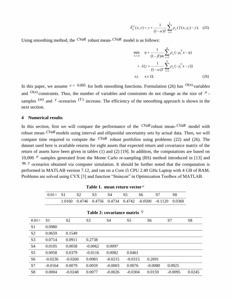
Table 1. mean return vector

0.01× S1 S2 S3 S4 S5 S6 S7 S8

1.0160 0.4746 0.4756 0.4734 0.4742 -0.0500 -0.1120 0.0360

Table 2: covariance matrix Q

0.01× S1 S2 S3 S4 S5 S6 S7 S8

S1 0.0980

S2 0.0659 0.1549

S3 0.0714 0.0911 0.2738

S4 0.0105 0.0058 -0.0062 0.0097

S5 0.0058 0.0379 -0.0116 0.0082 0.0461

S6 -0.0236 -0.0260 0.0083 -0.0215 -0.0315 0.2691

S7 -0.0164 0.0079 0.0059 -0.0003 0.0076 -0.0080 0.0925

S8 0.0004 -0.0248 0.0077 -0.0026 -0.0304 0.0159 -0.0095 0.0245

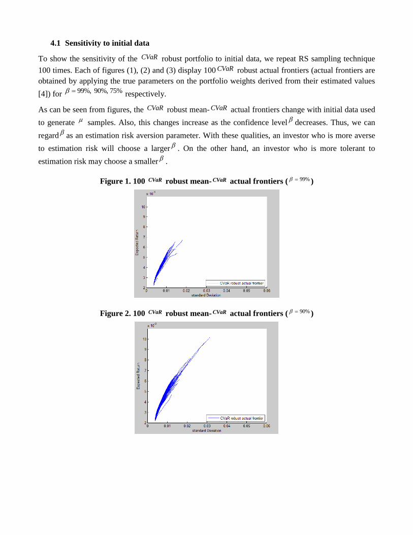
4.1 Sensitivity to initial data

To show the sensitivity of the CVaR robust portfolio to initial data, we repeat RS sampling technique

100 times. Each of figures (1), (2) and (3) display 100 CVaR robust actual frontiers (actual frontiers are

obtained by applying the true parameters on the portfolio weights derived from their estimated values

[4]) for 99%, 90%, 75% respectively.

As can be seen from figures, the CVaR robust mean- CVaR actual frontiers change with initial data used

to generate samples. Also, this changes increase as the confidence level decreases. Thus, we can

regard as an estimation risk aversion parameter. With these qualities, an investor who is more averse

to estimation risk will choose a larger . On the other hand, an investor who is more tolerant to

estimation risk may choose a smaller .

Figure 1. 100 CVaR robust mean- CVaR actual frontiers ( 99% )

Figure 2. 100 CVaR robust mean- CVaR actual frontiers ( 90% )

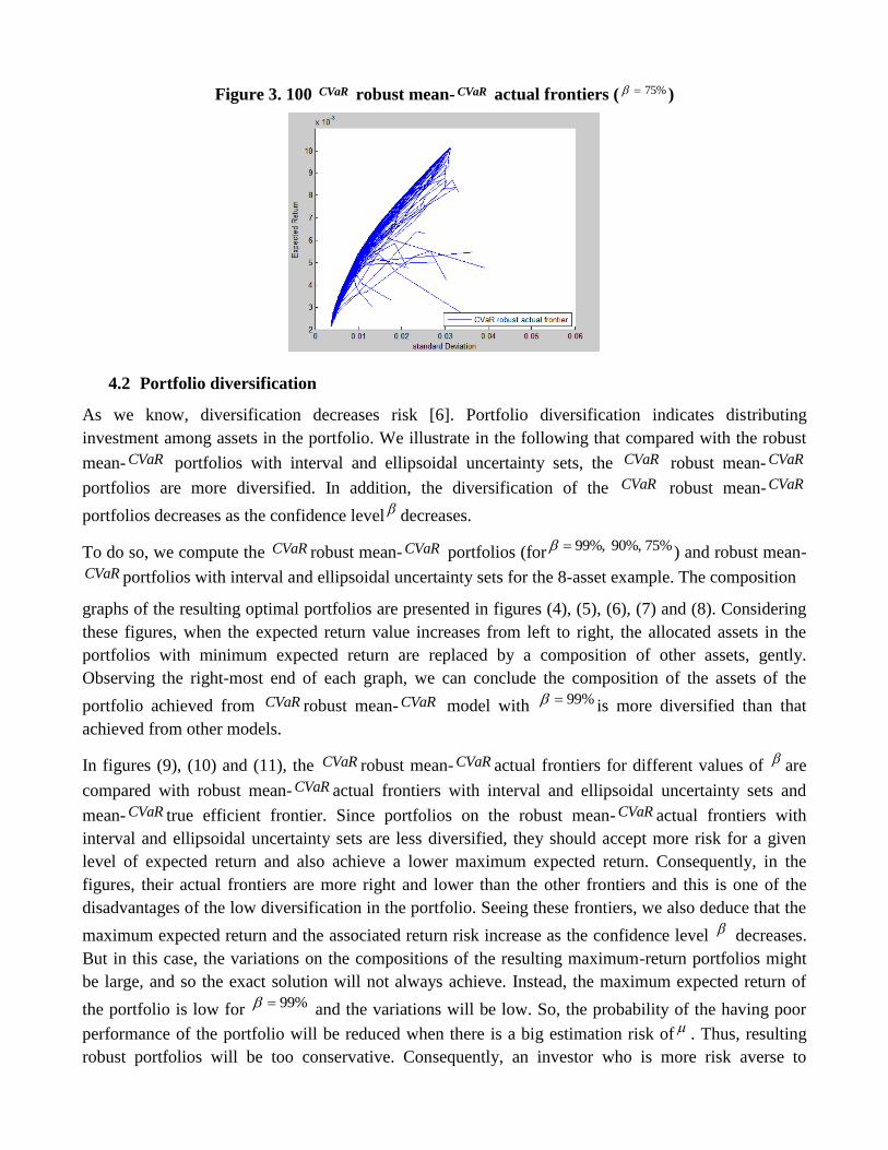
Figure 3. 100 CVaR robust mean- CVaR actual frontiers ( 75% )

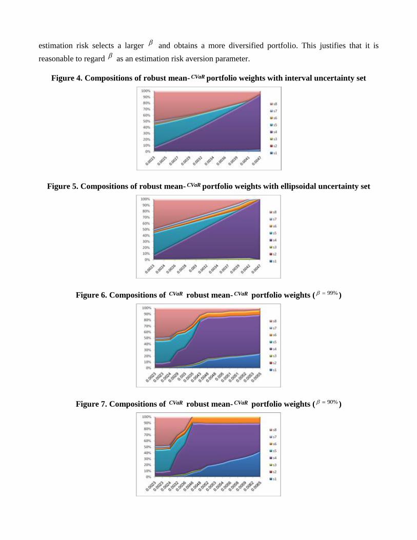
4.2 Portfolio diversification

As we know, diversification decreases risk [6]. Portfolio diversification indicates distributing

investment among assets in the portfolio. We illustrate in the following that compared with the robust

mean- CVaR portfolios with interval and ellipsoidal uncertainty sets, the CVaR robust mean- CVaR

portfolios are more diversified. In addition, the diversification of the CVaR robust mean-CVaR

portfolios decreases as the confidence level decreases.

To do so, we compute the CVaR robust mean- CVaR portfolios (for 99%, 90%, 75% ) and robust mean-

CVaR portfolios with interval and ellipsoidal uncertainty sets for the 8-asset example. The composition

graphs of the resulting optimal portfolios are presented in figures (4), (5), (6), (7) and (8). Considering

these figures, when the expected return value increases from left to right, the allocated assets in the

portfolios with minimum expected return are replaced by a composition of other assets, gently.

Observing the right-most end of each graph, we can conclude the composition of the assets of the

portfolio achieved from CVaR robust mean- CVaR model with 99% is more diversified than that

achieved from other models.

In figures (9), (10) and (11), the CVaR robust mean- CVaR actual frontiers for different values of are

compared with robust mean- CVaR actual frontiers with interval and ellipsoidal uncertainty sets and

mean- CVaR true efficient frontier. Since portfolios on the robust mean- CVaR actual frontiers with

interval and ellipsoidal uncertainty sets are less diversified, they should accept more risk for a given

level of expected return and also achieve a lower maximum expected return. Consequently, in the

figures, their actual frontiers are more right and lower than the other frontiers and this is one of the

disadvantages of the low diversification in the portfolio. Seeing these frontiers, we also deduce that the

maximum expected return and the associated return risk increase as the confidence level decreases.

But in this case, the variations on the compositions of the resulting maximum-return portfolios might

be large, and so the exact solution will not always achieve. Instead, the maximum expected return of

the portfolio is low for 99% and the variations will be low. So, the probability of the having poor

performance of the portfolio will be reduced when there is a big estimation risk of . Thus, resulting

robust portfolios will be too conservative. Consequently, an investor who is more risk averse to

estimation risk selects a larger and obtains a more diversified portfolio. This justifies that it is

reasonable to regard as an estimation risk aversion parameter.

Figure 4. Compositions of robust mean- CVaR portfolio weights with interval uncertainty set

Figure 5. Compositions of robust mean- CVaR portfolio weights with ellipsoidal uncertainty set

Figure 6. Compositions of CVaR robust mean- CVaR portfolio weights ( 99% )

Figure 7. Compositions of CVaR robust mean- CVaR portfolio weights ( 90% )

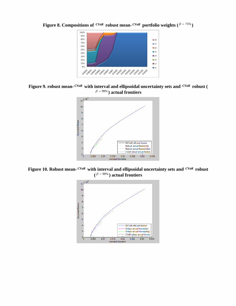
Figure 8. Compositions of CVaR robust mean- CVaR portfolio weights ( 75% )

Figure 9. robust mean- CVaR with interval and ellipsoidal uncertainty sets and CVaR robust (99% ) actual frontiers

Figure 10. Robust mean- CVaR with interval and ellipsoidal uncertainty sets and CVaR robust

( 90% ) actual frontiers

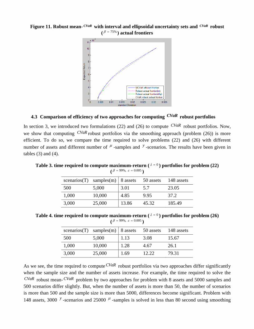
Figure 11. Robust mean- CVaR with interval and ellipsoidal uncertainty sets and CVaR robust

( 75% ) actual frontiers

4.3 Comparison of efficiency of two approaches for computing CVaR robust portfolios

In section 3, we introduced two formulations (22) and (26) to compute CVaR robust portfolios. Now,

we show that computing CVaR robust portfolios via the smoothing approach (problem (26)) is more

efficient. To do so, we compare the time required to solve problems (22) and (26) with different

number of assets and different number of -samples and y -scenarios. The results have been given in

tables (3) and (4).

Table 3. time required to compute maximum-return ( 0 ) portfolios for problem (22)

( 99%, 0.005 )

scenarios(T) samples(m) 8 assets 50 assets 148 assets

500 5,000 3.01 5.7 23.05

1,000 10,000 4.85 9.95 37.2

3,000 25,000 13.86 45.32 185.49

Table 4. time required to compute maximum-return ( 0 ) portfolios for problem (26)

( 99%, 0.005 )

scenarios(T) samples(m) 8 assets 50 assets 148 assets

500 5,000 1.13 3.08 15.67

1,000 10,000 1.28 4.67 26.1

3,000 25,000 1.69 12.22 79.31

As we see, the time required to compute CVaR robust portfolios via two approaches differ significantly

when the sample size and the number of assets increase. For example, the time required to solve the

CVaR robust mean- CVaR problem by two approaches for problem with 8 assets and 5000 samples and

500 scenarios differ slightly. But, when the number of assets is more than 50, the number of scenarios

is more than 500 and the sample size is more than 5000, differences become significant. Problem with

148 assets, 3000 y -scenarios and 25000 -samples is solved in less than 80 second using smoothing

technique, while by (22) it took over 185 seconds. These comparisons show that when the number of

scenarios and samples become larger, the smoothing approach is more computationally efficient to

determine CVaR robust portfolios than other approach.

References

S. Alexander‎, T.F. Coleman and Y. Li, “Minimizing VaR and CVaR for a portfolio of

derivatives,” ‎Journal of Banking and Finance‎, ‎Vol. 30, No. 2, 2006, pp. 583–605‎.

P. Artzner, F. ‎Delbaen‎‎, J. Eber and D. Heath, “Thinking coherently, ” Risk‎, Vol. ‎10, 1997, pp. 68–71‎.

S. Boyd and M. Grant, “Cvx users, guide for cvx version 1.21,” 2010. www.Stanford.edu/~boyd/cvx.

M. Broadie, “Computing efficient frontiers using estimated parameters,” Annals of Operations

Research, Vol. 45, 1993, pp. 21–58.

W.N. Cho‎, “Robust Portfolio Optimization Using Conditional Value At Risk‎,” ‎Imperial College

London‎, ‎Department of Computing‎, ‎Final Report, 2008‎‎‎.

G. Cornuejols and R. Tutuncu, “Optimization Methods in Finance,” ‎Cambridge ‎University Press, 2006.‎

L. Garlappi‎‎, R. ‎Uppal and T. Wang,‎ “‎Portfolio selection with parameter and model uncertainty‎: ‎A

multi-prior approach‎,” ‎Review of Financial Studies‎, Vol. ‎20, 2007, pp. 41–81‎‎.

D. Goldfarb‎‎ and ‎G. Iyengar, “Robust portfolio selection problems,‎” Mathematics of Operations

Research‎, ‎Vol. 28, No. 1, 2003, pp. 1–38‎‎‎.

S. Heusser, “Robust Mean-Modified Value at Risk Portfolio Optimization: An Empirical Application

with Hedge Funds, ” Diploma Thesis, University of Zurich, 2009.

P. Krokhmal, J. ‎Palmquist‎ and S. Uryasev, “Portfolio ‎o‎ptimization with ‎c‎onditional‎ V‎‎alue-at-‎R‎‎isk‎

o‎bjective and ‎c‎onstraints, ” Journal of Risk, ‎Vol. 4, 2002, pp. 43-48.

M. Letmark, “Robustness of Conditional Value at Risk when Measuring Market Risk Across Different

Asset Classes‎,” ‎Master Thesis‎, ‎Royal Institute of Technology‎,‎2010.

H. Markowitz, “Portfolio selection,” Journal of Finance‎, ‎Vol. 7, 1952, pp. 77–91‎‎.

R.O. Michaud, “Efficient Asset Management,‎” Harvard Business School Press, Boston, 1998.

A.G‎. Quaranta and A. Zaffaroni‎, “‎‎Robust Optimization of Conditional Value at Risk and Portfolio

Selection,‎” Journal of Banking and Finance‎, ‎Vol. 32, 2008, pp. 2046–2056‎.

R.T‎.‎ Rockafellar and S. Uryasev‎, “Optimization of conditional value-at-risk,” Journal of Risk‎, Vol. 2,

No. 3, 2000, pp. 21–41.

R.H. Tutuncu and M. Koenig, “Robust Asset Allocation,” Annals of Operations Research, Vol. 132,

2004, pp. 157-187.

J. Wang, “Mean-Variance-VaR Based Portfolio Optimization,” Valdosta State University, 2000.

L. Zhu, T.F. Coleman and Y. Li, “Min-max robust and CVaR robust mean-variance portfolios,”

Journal of Risk, Vol. 11, No. 3, 2009, pp. 1-31.

L. Zhu, “Optimal portfolio selection under the estimation risk in mean return,” MSc thesis, University

of Waterloo, Canada, 2008.