Lund University

School of Economics and Management

Department of Economics

Master thesis, October 2010

Exploring the properties of CVaR and

Mean-Variance for portfolio optimization

A comparative study from a practical perspective

Author: Peter Bengtsson Tutor: Hans Byström

1

Abstract

In this thesis some of the properties of Conditional Value at Risk and Mean-Variance for

portfolio optimization are explored, from a particularly practical perspective. The portfolio

optimizations are performed for data in two different time periods: 2006 and 2008. These

periods were chosen to capture both positive and negative financial market episodes, with

2006 representing a period of generally good results, while 2008 was a period dominated by

recession. The most important conclusion from this study is that there is a difference in how

the two risk measures under evaluation here perform under different market conditions. For

the settings imposed on this study, the MV portfolio is showing signs of state dependency.

However, even if the indications of state dependency are clear under these circumstances, the

results are not definitive. The finding is nonetheless interesting and should be further

investigated.

2

Contents

1. Introduction.............................................................................................................................3

1.1 Background.........................................................................................................................3

1.2 Purpose................................................................................................................................5

1.3 Outline.................................................................................................................................6

2. Portfolio Theory......................................................................................................................6

2.1 Market Risk……………………………………………………………………………….6

2.2 Minimum variance portfolio……………………………………………………………...7

2.3 Value-at-Risk......................................................................................................................9

2.4 Conditional Value-at-Risk………………………………………………………………..9

3. Methodology and data……………………………………………………………………...11

3.1 Data……………………………………………………………………………………...12

3.2 Methodology…………………………………………………………………………….12

3.2.1 Optimization of Conditional Value-at-Risk…………………………………………...13

3.2.2 Optimization of Global Minimum Variance Portfolio………………………………...16

3.2.3 Optimization constraints………………………………………………………………16

4. Results……………………………………………………………………………………...17

4.1 Results for 2006…………………………………………………………………………18

4.2 Results for 2008…………………………………………………………………………21

4.3 Comparison between the two periods…………………………………………………...23

5. Discussion and conclusion…………………………………………………………………25

References…………………………………………………………………………………….27

Appendix……………………………………………………………………………………...29

A. Weekly returns…………………………………………………………………………...29

B. Portfolio weights…………………………………………………………………………30

C. OMXS30…………………………………………………………………………………39

D. Matlab code………………………………………………………………………………40

3

1. Introduction

In the first section of the thesis I will describe the general background and history of portfolio

optimization. I also discuss the purpose of this study and outline the structure of the reminder

of the thesis.

1.1 Background

Measuring market risk is an important task for banks and other participants in the financial

markets, and in the light of the recent global financial market crisis, it is very topical.

Portfolio optimization has a long history which has been the subject of research and

discussion since the publication of Markowitz's seminal paper “Portfolio Selection” in 1952.

This showed how it was possible to generate investment portfolios which had the largest

expected return for a given level of risk (See, for example, Haugen, 2001). Markowitz's mean-

risk approach for portfolio selection use variance as a measure to describe the risk of the

portfolio (Markovitz, 1952). Although it is straightforward to compute the variance of a

portfolio, Markowitz highlighted several drawbacks, the most important being: that the

variance measure penalizes gains and losses symmetrically; and that it is not a suitable

measure to capture events of low probability, such as default risk. Despite the shortcomings of

the variance measure, Markowitz's paper has had a huge impact on the theory and practice of

portfolio optimization and risk management over the last 50 years.

It was not until 1994 and the introduction of the concept of Value-at-Risk (VaR) by

JP Morgan that a real alternative to the variance measure became available (See, for example,

Cheng, et al., 2004). VaR quickly became the standard for measuring market risk and the

Basel Committee for Banking Supervision recognised the role of the measure in determining

regulatory capital requirements (Basel Committee on Banking Supervision, 1996). It did not

take long, however, before questions were raised about the VaR measure's suitability for

portfolio optimization. Artzner, et al. (1997) introduced the concept of coherent risk

measures, based on a given risk measure's fulfilment of four axioms. It was shown that VaR

does not fulfil the sub-additivity axiom which implies that a portfolio's VaR might be higher

than the sum of its components. The lack of sub-additivity in the VaR measure, which goes

4

against the concept of diversification, and the fact that the optimization process with VaR is

complex, made the search for an alternative measure an important issue.

In this regard, Artzner, et al. (1997) proposed the use of a risk measure often called

Conditional Value-at-Risk (CVaR), otherwise known as Expected Shortfall (ES). This

measure is defined as the expected value of losses exceeding VaR. In other words, it is the

average of all the losses below the considered quantile (5% for the CVaR 95% which will be

used in this study). As opposed to the CVaR measure, the VaR measure does not tell you

anything about how bad things can get in the worst cases. Furthermore, Uryasev and

Rockafellar (1999) and Acerbi and Tasche (2001) have shown that CVaR fulfils the axioms of

coherence introduced by Artzner, et al. From its definition, it follows that the CVaR measure

will always be greater or equal to the VaR measure for a given portfolio, so, for example, a

portfolio with a low CVaR will also have a low VaR. Figure 1 illustrates the relationship

between VaR and CVaR.

Figure 1: VaR versus CVaR

Uryasev and Rockafellar (1999) developed a model for portfolio optimization under CVaR-

constraints using linear programming. This method is straightforward to use and has the

advantage of calculating a portfolio's VaR as a by-product. Furthermore, optimized CVaR

portfolios have been shown to be almost optimal in terms of VaR under this method.

Since its introduction, CVaR has been the subject of extensive research, which has primarily

aimed at understanding its properties. Uryasev and Rockafellar's (1999) model can compute

optimal portfolios under a number of different constraints. They have also shown that CVaR

is a coherent risk measure. CVaR's coherent properties were also investigated by Acerbi and

5

Tasche (2001) amongst others. Acerbi and Tasche concluded that CVaR were both coherent

and that it shared a lot of the advantages of VaR, for example it is universal and can be

applied to any instrument and any source of risk. In the literature, comparative studies of

CVaR's performance have for the most part focused on VaR.1 Yamai and Yoshiba (2002)

compare CVaR and VaR in three different aspects; estimation errors, decomposition into risk

factors and their performance in optimizations. They conclude that CVaR is easily

decomposed and optimized while VaR is not. De Giorgi (2002) study the efficient frontiers

obtained by solving the portfolio selection problem for CVaR, VaR and the variance. He

concludes that under the assumption of normal distribution the efficient frontiers obtained by

optimizing CVaR and VaR are subsets of the mean-variance efficient frontier. There have

also been studies about the CVaR measure's robustness and its properties for optimization of

hedge funds.

1.2 Purpose

The purpose of this thesis is to explore some of the properties of Conditional Value at Risk for

portfolio optimization, from a particularly practical perspective. The portfolios that are

computed by minimizing CVaR are compared to the Global Minimum Variance Portfolio.

Considering all the positive properties of CVaR and the known shortcomings of the variance,

it seems like an easy task to determine which one is best suited for portfolio optimization.

When one keep in mind that the situation is similar to when VaR was first introduced, the

solution to the problem might not be as clear as it first seemed. Mean-variance optimization is

straightforward, but how easy is it to use CVaR for portfolio optimization in practice? If the

two methods where used in practical application, which would present the best portfolios? A

large scale simulation would probably be the best way to fully understand the properties of the

methods, but given the complexity of undertaking such an exercise, and given the fact that the

results may not help understanding the practical use of the methods, this was beyond the

scope of this work. The aim of this study is to explore which method is best to use from a

practical point of view.

1 Although Tasche, et al. (2001) even go so far as to suggest that VaR is not a risk measure, since it does not fulfil the axioms of coherence.

6

1.3 Outline

The structure of the remainder of this thesis is as follows. In Section 2 some necessary

definitions are introduced, including that of market risk, along with the two methods of

portfolio optimization considered here. Section 3 provides a discussion of the methodology

used in the empirical analysis and also provides details of the data employed. Section 4

presents the results, while Section 5 completes the thesis with a discussion of the results and

conclusions.

2. Portfolio Theory

This section of the thesis introduces some important concepts and definitions that will be used

throughout the remainder of the work. It begins by discussing market risk before turning to

methods for portfolio optimization. Market risk is relevant for the topic of this thesis since it

plays a huge role during one of the time periods that are studied. Both the minimum variance

and Conditional Value at Risk methods are introduced in some detail. There is also a short

description of Value-at-Risk since it is extensively referred to throughout the thesis.

2.1 Market risk

Market risk, also known as systematic risk, is the risk that is common to an entire class of

assets or liabilities. Portfolios or other investments can suffer losses over a given time period,

due to macroeconomic impacts that broadly influence the financial markets. Market risk can

have a big impact on securities with high price volatility, while stable securities such as

treasury bills are not affected to the same extent (See, for example, Copeland et al., 2005).

Long term investments in securities are often not concerned since market risk fluctuates in a

cycle. As documented by the Basel Committee on Banking Supervision, there are primarily

four sources of market risk that may arise from the movement of market prices: interest rate

risk, foreign exchange risk, commodity position risk and equity position risk (Basel

Committee on Banking Supervision, 1996).

The development of the financial markets in recent years, with additional and more advanced

financial instruments, along with the globalisation of trading markets, has made market risk

7

an important issue for investors. Diversification remains the best method for protecting

against market risk, as this risk tends to affect different market segments at different times

(See, for example, Copeland et al., 2005). The latest financial crisis, however, affected many

market segments simultaneously, or at least sequentially. It is doubtful if diversification

would have had much effect in this rare event.

While the diversification of, for example, a portfolio of stocks may be intuitively appealing,

methods by which to choose a well diversified portfolio may not be so clear. Since Markovitz

(1952) showed how to create a frontier of portfolios, such that each of them had the biggest

feasible return given their level of risk, a large number of risk measures have been used and

then rejected when their shortcomings were exposed. Regardless of which method to use, all

risk managers seem to agree that diversification is the best way to reduce risk. There is,

however, decreasing returns to diversification. In a well balanced stock portfolio the risk is

reduced when you add another stock, but when the portfolio has reached about 20 stocks, the

portfolio approaches optimal diversity (see, for example, Elton and Gruber, 2006). This

implies that risk can only be reduced to a certain degree, after which there is no further benefit

from diversification.

2.2 Minimum variance portfolio

Even though portfolio optimization and risk management have progressed significantly since

the introduction of Markowitz’s framework, methods that are typically employed are still

based on the mean-risk approach introduced in that framework. Mean-variance optimization,

as developed by Markowitz, aims to find the set of optimal portfolios which have the highest

rate of return for a given level of risk. The portfolio with the lowest level of risk is referred to

as the Global Minimum Variance Portfolio. Finding the Global Minimum Variance Portfolio

is rather straightforward, as it is the solution to the following minimization problem (See, for

example, Kempf and Memmel, 2002):

(2.1)

8

where is a column vector of ones and is a vector of portfolio weights and

is the covariance matrix of the returns. The weights of the

global minimum variance portfolio are given by:

(2.2)

The expected return and the portfolio variance of the Global Minimum Variance Portfolio are

given by:

(2.3)

and

(2.4)

The MVP method is easy to understand and straightforward to compute, and these features

enhance its appeal. The method has some important drawbacks, and from a practical

perspective, it is important that these are well understood and that results derived from the

methods are seen in the context of these limitations. Most importantly the variance measure

symmetrically penalizes gains and losses, which from a risk management perspective may not

be optimal. Furthermore, the method is not suitable to describe events of low probability, such

as default risk (See, for example, Copeland et al., 2005).

Despite these shortcomings, the Global Minimum Variance portfolio method has been

frequently preferred for portfolio optimization in recent years. This is due to the fact that

expected portfolio returns are difficult to estimate and that estimation errors can lead to sub-

optimal portfolio selection (Jorion, 1991). By assuming that all stocks have the same expected

returns, all stock portfolios differ only with respect to their risk. The Global Minimum

Variance portfolio depends only on the covariance matrix of stock returns. This covariance

matrix can be estimated much more precisely than expected returns (See, for example, Kempf

and Memmel, 2002). Given the assumption that all stocks have the same expected returns, and

the further assumption that variance is an appropriate measure of risk, the Global Minimum

9

Variance portfolio will be the only efficient stock portfolio. This makes this method very

powerful, notwithstanding the assumptions outlined.

Despite the power of the MVP approach, other methods have gained in importance in recent

times and have increasingly been used in practical applications. In this regard, value-at-risk

has been the most prominent.

2.3 Value-at-Risk

Value-at-Risk (VaR) can be defined as the maximum loss not exceeded with a given

probability defined as the confidence level, over a given period of time (Jorion 1997). Under

the assumption that the portfolio return is normally distributed, VaR for the 95% confidence

level is given by:

(2.5)

Where pV is the initial value, pµ is the expected value and pσ the standard deviation.

VaR was first introduced 1994 by JP Morgan and its use quickly spread. VaR was soon to be

considered the standard for measuring market risk and it seemed that there finally was a risk

measure that did not share the limitations of the variance measure. The Basel Committee for

Banking Supervision, therefore, recognised the role of the measure in determining regulatory

capital requirements. VaR is easy to understand and simplify risk analysis, making it

attractive for risk managers. It only took a few years, however, before concern was raised

over some of VaR:s properties. As described in previous sections, Artzner et al. (1997)

showed that VaR does not fulfil the sub-additivity axiom, which implies that a portfolio's VaR

might be higher than the sum of its components. Artzner and the axioms will be further

discussed in the next section.

2.4 Conditional value-at-risk

Conditional value-at-risk (CVaR) is an alternative measure of expected loss that was

introduced by Uryasev and Rockafellar (1999). The measure is considered to be more

consistent than VaR and is measuring the expected loss given that the loss is greater than

10

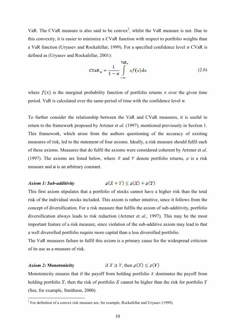
VaR. The CVaR measure is also said to be convex2, whilst the VaR measure is not. Due to

this convexity, it is easier to minimize a CVaR function with respect to portfolio weights than

a VaR function (Uryasev and Rockafellar, 1999). For a specified confidence level CVaR is

defined as (Uryasev and Rockafellar, 2001):

(2.6)

where is the marginal probability function of portfolio returns over the given time

period. VaR is calculated over the same period of time with the confidence level .

To further consider the relationship between the VaR and CVaR measures, it is useful to

return to the framework proposed by Artzner et al. (1997), mentioned previously in Section 1.

This framework, which arose from the authors questioning of the accuracy of existing

measures of risk, led to the statement of four axioms. Ideally, a risk measure should fulfil each

of these axioms. Measures that do fulfil the axioms were considered coherent by Artzner et al.

(1997). The axioms are listed below, where and denote portfolio returns, is a risk

measure and is an arbitrary constant.

Axiom 1: Sub-additivity

This first axiom stipulates that a portfolio of stocks cannot have a higher risk than the total

risk of the individual stocks included. This axiom is rather intuitive, since it follows from the

concept of diversification. For a risk measure that fulfils the axiom of sub-additivity, portfolio

diversification always leads to risk reduction (Artzner et al., 1997). This may be the most

important feature of a risk measure, since violation of the sub-additive axiom may lead to that

a well diversified portfolio require more capital than a less diversified portfolio.

The VaR measures failure to fulfil this axiom is a primary cause for the widespread criticism

of its use as a measure of risk.

Axiom 2: Monotonicity if , then

Monotonicity ensures that if the payoff from holding portfolio dominates the payoff from

holding portfolio , then the risk of portfolio cannot be higher than the risk for portfolio

(See, for example, Smithson, 2000).

2 For definition of a convex risk measure see, for example, Rockafellar and Uryasev (1999).

11

Axiom 3: Translation invariance

Translation invariance axiom requires that the addition of liquid cash, and therefore risk free

assets to a portfolio, reduces the risk of the portfolio accordingly.

Axiom 4: Positive homogeneity

Positive homogeneity implies that the portfolio risk always is related to the size of the

portfolio.

These axioms have come to be considered the minimum standard for any risk measure. The

failure to fulfil any one axiom could likely lead to incorrect results, and therefore, inferences

being drawn from a particular risk measure (See, for example, Acerbi and Tasche, 2001). The

CVaR measure has been proven to be coherent and is, therefore, a good alternative to the use

of VaR and perhaps MVP (see Acerbi and Tasche, 2001). Uryasev and Rockafellar (1999)

have developed a model for portfolio optimization under CVaR-constraints using linear

programming. This method is easy to use and will be further explored under the methodology

section.

3. Methodology and data

This section provides an overview of the methods used to comparatively assess the relative

practical performances of the MVP and CVaR methods in portfolio optimization, as outlined

in Section 1. This section also provides details of the data employed for the computation of

the portfolios. In order to explore some of the properties of Conditional Value at Risk for

portfolio optimization, a range of suitable data was gathered and a suitable methodological

approach set out. Details of both are provided in this chapter, which first discusses data and

related issues. Recall that a key aim of this project is to evaluate the relative performance of

the portfolio optimization methods from a practical perspective. Details of the methodological

approach taken are then outlined. In particular, the novel approach taken to overcome the

challenges in comparing the minimum variance approach - which requires just returns data –

and the CVaR method - which also requires a target return level – is explained in some detail.

12

3.1 Data

To implement this methodology in comparatively assessing the relative practical

performances of the MVP and CVaR methods in portfolio optimization, data from Thompson

Financial Datastream was gathered. Specifically, time series data for ten stocks, quoted on the

Stockholm Stock Exchange, were obtained, from which portfolios were constructed. As the

data provider is reputable and the source is widely used in both academic and practical

applications, the quality of the data was deemed to be sufficient. Nevertheless, rudimentary

checks of the data were undertaken to ensure its quality and the absence of errors and outliers.

The criteria by which the ten stocks were chosen ensured that different stock-market segments

were represented. To some extent, this gave the resultant portfolios a degree of

diversification. For each, a time series of daily stock prices was obtained, for each of two

distinct time periods, to allow for the comparative performance of the risk measures to be

gauged over different time periods. The stock prices were converted to daily returns, which

formed the basis for the portfolio optimizations.

The stocks included were those of: Alfa Laval, ABB, Axfood, Elektrolux, Ericsson, Investor,

Nordea, Skanska, Swedish Match and Volvo. They were chosen to represent different

segments of the stock market. For the first time period studied, all stocks generated a positive

rate of return. The highest rate of return was attributable to Alfa Laval, at almost 67 per cent,

while at the other end, Ericsson’s rate of return was just 4 per cent. During the second period

included in the study, all stocks generated negative rates of return, in light of the economic

climate during that year. The worst result for 2008 was Volvo, which lost more than 74 per

cent. The next section describes the methodological approach used for this study.

3.2 Methodology

The portfolio optimizations were performed for data in two different time periods: 2006 and

2008. These periods were chosen to capture both positive and negative financial market

episodes, with 2006 representing a period of generally good results, while 2008 was a period

dominated by recession. Including such relatively distinct periods ensures that general

differences in the methods related to the data characteristics were observed and controlled.

Furthermore, two estimation windows were also employed: 125 trading days and 250 trading

13

days, which correspond to six months and twelve months of historical daily returns. The

Swedish Financial Supervisory Authority recommends an estimation window of at least

twelve months, given that low probability events should not impact significantly on portfolio

weights (Finansinspektionen, 2004). Nevertheless, the estimation windows used here are

deemed to be sufficient, as 1) the study has a practical focus and understanding the methods’

characteristics for shorter periods may be of practical interest; and 2) comparing longer

periods may render differences between the methods more difficult to observe.

For each data sample, the resultant portfolio was rebalanced weekly, giving 208 portfolios

from minimizing the variance, 208 portfolios from minimizing conditional Value-at-Risk and

a total of 416 portfolios. The portfolio weights derived in each case were used to calculate the

weekly returns for actually holding each portfolio during the periods of time considered. This

allows for a practical comparison to be made between the two very different methods for

portfolio optimization. In terms of comparison, both the level of returns, as well irregularities

between the two different sets of portfolio returns were considered.

The model derived by Uryasev and Rockafellar (1999) for portfolio optimization under

CVaR-constraints requires a target return level as an input in order to compute the optimal

portfolio weights. This requirement makes the comparison with the minimum variance

portfolio, which requires just returns data, difficult from a practical perspective. To make a

comparison possible, a novel approach was taken. Rather than computing the optimized

portfolio weights using CVaR for a specific target return, the procedure was nested; that is,

the portfolio optimization was conducted within another optimization framework, which

sought to minimise the level of CVaR for a given portfolio across a range of return levels.

This approach avoided the need to choose a particular target return level a priori and ensured

that the results obtained from CVaR were not unduly influenced by the choice of target return

value. The next section elaborates in detail on how the CVaR portfolios were optimized

within this nested procedure.

3.2.1 Optimization of CVaR

Rockafellar and Uryasev (1999) developed a method for the optimization of CVaR portfolios

and it is this method which will be used in this thesis. With their approach, the optimization

14

problem can be solved with linear programming of a smooth and convex function. This

section elaborates on the derivation of the function to be minimised and details the constraints

that will be used in the practical application reported on in Sections 4 and 5. Further details on

Rockafellar and Uryasev’s (1999) results can be found in selected papers detailed in the

reference list. The following exposition is largely based on Rockafellar and Uryasev (1999)

and Uryasev (2000).

Let be the loss associated with the decision vector , itself chosen from the specific

subset of and the random vector in . Then, the vector can be interpreted as

representing a portfolio, with as the set of obtainable portfolios. The underlying probability

distribution of , represented by the density function , and the probability of , not

exceeding some threshold , is given by:

(3.1)

where , as a function of for fixed , is the cumulative distribution function for the loss

related with portfolio . is non-decreasing with respect to and, as with , is also

continuous. The VaR and CVaR values can be denoted as and respectively and

in Rockafellar and Uryasev's (1999) settings they are given by:

, (3.2)

and

(3.3)

The CVaR function in Equation 3.3 is difficult to handle, as it is a function of the VaR

function. Using for the optimization of CVaR implies that VaR would have to first be

calculated. The primary contribution by Rockafellar and Uryasev (1999) was the derivation of

a CVaR function that was independent of the VaR function, making the optimization process

much less complicated. Their function is given by:

15

(3.4)

where

which can be used instead of the CVaR measure. It has been proved that the function

is convex with respect to α and that minimizing the function gives the same result as solving

(Uryasev and Rockafellar, 1999).

(3.5)

This follows from the derivative of the function with respect to equals:

(3.6)

the proof of which can be found in Uryasev and Rockafellar (1999). By equating this

derivative to zero, it is possible to find the VaR that minimizes the function with

respect to . From this, it follows that the minimization of the function with respect to both

variables optimizes CVaR, and at the same time, delivers VaR as a by-product. This

simplification of the CVaR function makes the optimization problem much easier, as there is

no need to calculate the portfolio’s VaR measure. A more detailed explanation of the

derivation of the method is available in Rockafellar and Uryasevs papers, which are detailed

in the reference list.

From a practical perspective, the optimizations are carried out using Matlab. The code is

based on an existing program, which has been adapted to suit the work conducted here.3

Furthermore, the portfolios were minimized with respect to the CVaR measure for .

No short sales were permitted in the analysis and individual portfolio weights were restricted

to less or equal to 25 per cent of the entire portfolio. The later constraint ensures a degree of

diversification in the optimized portfolios.

3 Link to original code: http://www.mathworks.com/matlabcentral/fileexchange/19907

16

3.2.2 Optimization of Global Minimum Variance Portfolio

Optimizing the Minimum Variance Portfolio simply requires minimizing the variance of the

portfolio, subject to a number of constraints. This optimization problem is quite

straightforward and is well understood. Details concerning this approach are not, therefore,

elaborated here; just a short description of the approach employed is provided.

Mathematically, the minimization problem can be stated as:

(3.7)

where is an column vector of portfolio weights and is the covariance matrix

of returns. Optimizations to obtain the minimum variance portfolios were also carried out in

Matlab.4 This code included the constraints presented in the next subsection.

3.2.3 Optimization constraints

The same set of constraints was applied to all portfolios and implemented for both

methodological approaches, to ensure comparability in the outputs. The first constraint, which

ensures that short sales are not permitted, can be formulated as:

(3.8)

There are several reasons to impose this constraint. The most important, from a practical point

of view, is the many regulations concerning short sales in financial markets around the world.

For example, the short sale of a particular stock is, in many cases, not permitted once the price

of that stock has already started to decline.

The second restriction to be imposed is intuitive, since it ensures that the portfolio weights

sum to unity:

4 The Matlab code for optimizing the minimum variance portfolios, written by the author, was tested to ensure accuracy and reliability, and is available in the appendix.

17

(3.9)

The final mutual constraint:

(3.10)

ensures that no portfolio weight exceeds 25 per cent. This constraint imposes a degree of

diversification in the optimized portfolios. For portfolios constructed by minimizing CVaR, a

confidence level was also required. The most common levels of confidence chosen are

typically 90 per cent, 95 per cent and 99 per cent. For this study, the 95 per cent level was

chosen. Just one level was used to simply the exercise and to keep the number of portfolios to

a manageable level.

4. Results

In this section the results of the study are presented. The outputs from the study consist of

portfolios, based on the two methods under evaluation, and portfolio weights for each stock

included in the data sample. From these, rates of return for the optimized portfolios, in the

form of weekly returns, expressed in percentage terms, were calculated. These rates of return

are presented in Appendix.

The design of the study allows for multiple comparisons of the CVaR and MVP methods to

be made. First, the results derived from both methods are compared for 2006 and then 2008.

This comparison includes two estimation windows for each year.5 The aim of this comparison

is to evaluate the relative performance of the risk measures. Further comparisons between the

measures can be drawn by comparing performances across the two different periods, 2006

and 2008, given the very different characteristics of those periods. This adds a further

dimension to the comparative study, which may reveal a degree of state dependency in the

measures’ performance, i.e., the performance of the measures may be impacted by the

contemporary state of some exogenous factor, such as the general condition of financial

5 As described in Section 3, the optimizations were carried out for estimation windows of 125 and 250 trading days, which corresponds to six months and twelve months, respectively, of historical daily returns.

18

markets. While such results could not hope to be definitive, based on the comparison of just

two years, it may reveal or at least hint at some state dependency. Such a finding would,

notwithstanding its tentative nature, be extremely interesting and relevant. In making a

comparison, however, there is little to gain from comparing the absolute levels of the

optimized portfolios returns over the periods chosen, given the very different characteristics

of those periods. By making comparisons with the OMXS30 index, however, it is possible to

obtain an indication of the measures relative performance.6

4.1 Results for 2006

The year 2006 was a generally favourable period in terms of stock market returns: the rate of

return for most stocks was positive. Unsurprisingly, therefore, both the portfolio sets that

result from the MVP and CVaR selection methods yielded a significant return for the period

as a whole. Despite the fact that both sets of portfolios are constructed by minimizing their

respective risk measure, it is interesting to note that they both outperformed the OMXS30

index over the period.

The MVP method yielded a total rate of return of 34 per cent for the shorter estimation

window and 32 per cent for the longer window. These results refer to the whole period

studied, although weekly rates of return can be found in Appendix A. These results suggest

that the length of the estimation window, at least under these circumstances, does not appear

to affect the result to a great extent. The shorter estimation window did, however, provide a

rate of return approximately 2 per cent higher than the longer window, and while the

statistical significance of this result could not be considered here, in financial applications

even relatively small differences may be significant from a practical perspective. During this

period, the OMXS30 index yielded a return of 19 per cent. It is notable that the MV portfolios

offered a much higher return than the index, since they are, at least in theory, less risky. The

reason is not, however, that the composition of the index differed from the stocks chosen for

this study. Of the ten stocks selected for inclusion in this study, nine were included in the

index during 2006. The explanation of the significant difference in rate of return can be found

in the method by which the portfolio weights of the stocks were chosen. The index is value

6 The OMXS30 is a market value weighted index that consists of the 30 most traded stocks on Stockholm Stock Exchange. The composition of stocks is changed twice each year, based on the previous six months of trading. Usually, however, there is little or no change in the composition of stocks.

19

weighted, while the MV portfolios’ weights were chosen to minimize the portfolios’ variance.

This means that the index at all times is made up of different weights of all the 30 constituent

stocks, whereas the MV portfolios’ composition, under the constraints imposed in this study,

can vary between four and all ten stocks. The consequence is that the MVP method results in

a more rapid reaction to changes in the return of individual stocks.

The CVaR portfolio yielded a total rate of return of 27 per cent for the shorter estimation

window and 24 percent for the longer estimation window. As for the MVP, these results refer

to the entire period studied. Once again, the length of the estimation window, as indicated by

the returns, appears to have a small but significant impact on the relative performance of the

risk measure used for the optimizations. In this case, the shorter estimation window results in

a more than 3 per cent increase in the total rate of return. A comparison with the OMXS30

index shows that the CVaR portfolio yielded a higher return, and even though the difference

is not very large, it is nonetheless significant. To explain this difference in rate of return, the

same analysis outlined in the previous paragraph, can be applied. The difference relates to the

method by which the portfolio weights were chosen and the constraints imposed on the CVaR

portfolio, as well as the index.

On the basis of these results, it is clear that the MVP method out-performs the CVaR method

during the period studied and for this selection of data. This result remains regardless of

whether the portfolios were computed on the basis of an estimation window of 125 or 250

trading days. For both estimation window lengths, the MV portfolios yielded a larger rate of

return than the CVaR portfolios. As can be observed in figures 4.1 and 4.2, the weekly returns

do not vary much between the different portfolios for most weeks. The most significant

difference is that: 1) the CVaR portfolios show more weeks with large losses; and 2) that

these losses are larger than those of the MV portfolios. For both estimation window lengths,

the MV portfolios generate a higher rate of return in just 56 per cent of the weeks studied,

which implies that the large difference in yearly rate of return is due to the large losses for the

CVaR portfolios. This is noteworthy and will be discussed further in the next section.

20

Figure 4.1

2006 125-days estimation window

-0,08-0,06-0,04-0,02

00,020,040,06

1 4 7 10 13 16 19 22 25 28 31 34 37 40 43 46 49 52

MVP

CVaR

Figure 4.2

2006 250-days estimation window

-0,08

-0,06

-0,04

-0,02

0

0,02

0,04

0,06

1 4 7 10 13 16 19 22 25 28 31 34 37 40 43 46 49 52MVP

CVaR

It should also be mentioned that the weekly returns for both sets of portfolios show a

relatively high volatility, something that may stem from the length of the estimation window

used. The volatility may be less significant for a larger estimation window, as discussed in the

methodology section. As also mentioned in that section, such a reduction in volatility may

come at the expense of highlighting the differences between the two methods used for

portfolio selection in this study.

Having compared the performances of both risk measures with data from 2006 - a relatively

positive period for financial markets - the next section describes the results obtained for a very

different period, 2008, which was dominated by financial crisis.

21

4.2 Results for 2008

The second period chosen for this study, 2008, was dominated by financial crisis. It may be

argued that 2008 represented the worst period of the crisis to date, as it spread from money

markets in late summer 2007 to affect financial markets more broadly. That year saw the

rescue-takeover of Bear Stearns and the bankruptcy of Lehman Brothers, two large and

important financial institutions in the United States. Risk aversion in financial markets

reached high levels with few if any sectors escaping as many global economies entered

recession. Not until March 2009 did a recovery in stock markets generally take hold. As a

result, the period chosen for this aspect of the study was one that can be characterised by

falling stock prices and provides an excellent example of the effects of a materialisation of

market risk. Due to macroeconomic impacts, many market segments were simultaneously

affected. In light of the economic climate, it is unsurprising, therefore, that both sets of

portfolios derived from the methods under examination yielded large losses during this

period. In contrast to the previous period studied, however, a much larger difference was

observed between the portfolios optimized with an estimation window length of 125 days and

those minimized using an estimation window length of 250 days. The longer estimation

window generated better results for both methods of portfolio optimization studied.

The MVP method yielded a total rate of return for the whole period of -38 per cent for the

shorter estimation window and -32 per cent for the longer estimation window, a difference of

more than 6 per cent. This is intuitive, since historical observations during the financial crisis

period had a greater impact when the shorter estimation window length was used for the

optimizations. A comparison with the OMXS30 index, which had a total rate of return of -38

per cent over the period, shows that the MV portfolios computed with the longer estimation

window yielded a significantly higher rate of return than the index. The portfolios derived

from the shorter window performed similarly to the index. As for the previous period studied,

nine of the ten stocks selected for the optimizations were included in the index during 2008. It

is surprising, therefore, that the optimized portfolios derived from the longer window showed

a much higher rate of return than the index. In figures 4.3 and 4.4, a very large loss for the

MV portfolio can be seen in Week 41. This loss is about 21 per cent for both estimation

window lengths. It can most likely be explained by the bankruptcy of the large US investment

bank Lehman Brothers in September of that year.

22

Figure 4.3

2008 125-days estimation window

-0,25-0,2

-0,15-0,1

-0,050

0,050,1

0,15

1 4 7 10 13 16 19 22 25 28 31 34 37 40 43 46 49 52MVPCVaR

Figure 4.4

2008 250-days estimation window

-0,25-0,2

-0,15-0,1

-0,050

0,050,1

0,15

1 4 7 10 13 16 19 22 25 28 31 34 37 40 43 46 49 52MVPCVaR

The portfolio obtained by minimizing the CVaR measure yielded a total rate of return of -39

per cent for the shorter estimation window and -34 per cent for the longer estimation window,

a difference of almost 5 per cent. The results are similar to those of the MVP, in regard to the

difference in rates of return between the two estimation window lengths. As discussed earlier,

this discrepancy in the rates of return can be expected when historical observations during the

financial crisis period are given a greater weight. When compared to the OMXS30 index, the

longer estimation window shows a much higher rate of return, while the shorter window

performed slightly worse than the index. The large loss during Week 41 due to the bankruptcy

23

of Lehman Brothers that could be observed for the MVP, was also present for the CVaR

portfolio.

Even though the difference between the MV and CVaR portfolios is less significant than that

observed for 2006, the MV portfolios still show somewhat better returns for both estimation

window lengths. The most important finding in comparing the performance of the risk

measures during this period is that the difference in rates of return is much smaller than

during the previous period studied. This may reveal a degree of state dependency in the

measures’ performance which will be further discussed in the next section. Another

interesting result is the large difference observed between the two estimation windows used,

even if this can be explained by the fact that historical observations during the financial crisis

period had a greater impact on the optimizations using shorter estimation window length. In

figures 4.3 and 4.4, it can be observed that the CVaR portfolios result in a higher number of

weeks with large losses and since this is the case for both periods under examination, it will

be addressed in the next section.

Having completed the analysis for both the 2006 and 2008 periods individually, the next

section considers the relative performance of the risk measures across both periods, with a

view to understanding how the measures may perform in different financial market ‘states’.

4.3 Comparison between the two periods

The main purpose of this study was to observe differences, if any, in how the two sets of

optimized portfolios performed under different market conditions. To ensure that the financial

market conditions where sufficiently diverse, the first period chosen was characterised by

flourishing stock markets, while the second period was dominated by financial crisis. This

gives the comparative study a further dimension, which may reveal a degree of state

dependency in the measures’ performance, i.e., the performance of the measures may be

impacted by the contemporary state of some exogenous factor, such as the general condition

of financial markets.

The MVP method yielded a total rate of return for 2006 of 34 per cent for the shorter

estimation window and 32 per cent for the longer window. During this period, the OMXS30

24

index yielded a return of 19 per cent. This difference in rate of return is significant and, as

discussed in previous sections, noteworthy for obvious reasons. For the second period studied,

the MVP method yielded a total rate of return of -38 per cent for the shorter estimation

window and -32 per cent for the longer estimation window. A comparison with the OMXS30

index, which had a total rate of return of -38 per cent over the period, shows that the MV

measure and the index yielded a similar result for 2008. The comparison with the index

reveals a significant difference in the MV portfolios performance during the two periods

studied. The relative performance of the MV measure is much better during the first period

included in the study, than during the financial crisis that characterizes the second period.

Even though this result is indicative only and in no way definitive, being based on the

comparison of just two years, it does at least hint towards the existence of some state

dependency. The difference is significant and is present for both estimation window lengths.

The CVaR portfolio yielded a total rate of return for 2006 of 27 per cent for the shorter

estimation window and 24 percent for the longer estimation window. A comparison with the

OMXS30 index shows that the CVaR portfolio yielded a higher return, and even though the

difference is not very large, it is nonetheless significant. For 2008, the portfolio obtained by

minimizing the CVaR measure, yielded a total rate of return of -39 per cent for the shorter

estimation window and -34 per cent for the longer estimation window. This reveals that the

CVaR measure’s relative performance is, as was the case for the MV portfolio, better during a

favourable period for stock market returns. The difference in performance is, however, not as

significant as for the MV measure. Market conditions appear to have a somewhat lesser affect

on the performance of the CVaR measure. Furthermore, it should be noted that the CVaR

portfolios contain more weeks with large losses, a result which holds for both periods. This

will be discussed further in the final section of the thesis.

The most important finding, in comparing the relative performance of the risk measures

across the two periods of time, is the very different results for the MV portfolio. This

indicates the existence of some degree of state dependency in the measures performance, and

is an interesting finding. This implies that the relative performance of the MV measure is

impacted by the general condition of financial markets, and therefore, its suitability for use

may be questioned under certain market conditions. The result is, however, not definitive as it

25

is based on the comparison of just two years of data; further investigation in this regard is

warranted.

Having completed the analysis of the relative performance of the risk measures across both

periods, the next section concludes the thesis and attempts to interpret more carefully the

results of the optimizations.

5. Discussion and conclusion

The purpose of this thesis was to explore some of the properties of Conditional Value at Risk

for portfolio optimization, from a mainly practical perspective. The portfolios that were

computed by minimizing CVaR were compared to the Global Minimum Variance Portfolio.

The portfolio optimizations were performed for two different time periods: 2006 and 2008.

These periods were chosen to capture both positive and negative financial market conditions,

with 2006 representing a period of favourable results, while 2008 was dominated by

recession. Including such distinct periods ensured that general differences in the methods

related to the data characteristics were observed and controlled.

The results for 2006 show that both portfolio sets yielded a significant return for the period as

a whole. Even though the positive rate of return was expected, considering the settings, it is

interesting to note that they both outperformed the OMXS30 index over the period. The most

significant difference between the two sets of optimized portfolios over the period was that

the CVaR portfolios showed more weeks with large losses, and that these losses are larger

than those of the MV portfolios. In contrast to the previous period studied, 2008 was a year of

widespread recession and that was reflected in the optimized portfolios. Both sets of

portfolios derived from the methods under examination here yielded large losses during this

period. The difference between the MV and CVaR portfolios were less significant than for

2006, but the MV portfolios still showed somewhat better returns for both estimation window

lengths. The most important finding during this period was that the difference in rates of

return was much smaller than during the previous period studied.

26

Two estimation windows were employed for the optimizations, 125 trading days and 250

trading days, which correspond to six months and twelve months of historical daily returns.

The length of the estimation window does not seem to have a significant impact on the results

of the optimizations, even though there is a small difference for the second period under

evaluation. As discussed earlier, this difference might stem from the fact that historical

observations during the financial crisis period had a greater impact on the optimizations using

a shorter estimation window length. The most important consequence of the choice of

estimation window length may be the rather high volatility shown by both sets of portfolios.

A longer estimation window could have reduced the volatility; however, such a reduction in

volatility could have come at the expense of highlighting the differences between the two

methods used in this study. The conclusion to be drawn is that the choice of estimation

window length has a small, but nonetheless significant, effect on the result of the

optimizations.

As outlined in previous sections, the main purpose with this study was to observe if there

were any differences in how the two sets of optimized portfolios performed under different

market conditions. The most interesting discovery, when comparing the relative performance

of the risk measures across the two periods of time, was the significant difference in rate of

return for the MV portfolio. This may point to a degree of state dependency in the measures

performance, and is an extremely interesting finding. From a practical perspective, this result

implies that the performance of the MV measure is impacted by the general condition of

financial markets, and therefore, is more suited as a measure of risk under specific market

conditions. For this selection of data, and with the constraints imposed for the optimizations

in this study, the MV method’s relative performance is superior during favourable market

conditions. The reason for this is beyond the scope of this work, but might be due to the way

the MV measure penalizes gains and losses symmetrically.

The most important conclusion from this study is that there is a difference in how the two risk

measures under evaluation here perform under different market conditions. For the settings

imposed on this study, the MV portfolio is showing signs of state dependency. However, even

if the indications of state dependency are clear under these circumstances, this study is based

on the comparison of just two years, and therefore the results are not definitive. The finding is

nonetheless interesting and should be further investigated.

27

References

Printed Sources

Copeland, Thomas; Shastri, Kuldeep and Weston, Fred (2005). Financial Theory and

Corporate Policy. Pearson Education. USA

Elton, Edwin and Gruber, Martin (2006). Modern Portfolio Theory and Investment Analysis.

John Wiley & Sons. USA.

Haugen, Robert (2001). Modern Investment Theory. Prentice Hall, New Jersey, USA.

Jorion, Philippe (1997). Value at Risk. McGraw-Hill. USA

Articles

Acerbi, Carlo and Tasche, Dirk (2001). Expected Shortfall: a natural coherent alternative to

Value at Risk.

Artzner, Philippe; Delbaen, Freddy; Eber, Jean-Marc and Heath, David (1997). Thinking

Coherently. Risk Vol. 10

Artzner, Philippe; Delbaen, Freddy; Eber, Jean-Marc and Heath, David (1999). Coherent

Measures of Risk. Mathematical Finance Vol. 9 No 3.

Cheng, Siwei; Liu, Yanhui and Wang, Shouyang (2004). Progress in Risk Measurement.

AMO – Advanced Modelling and Optimization, Vol. 6.

De Giorgi, Enrico (2002). A Note on Portfolio Selection under Various Risk Measures.

Finansinspektionen (2004). Intern VaR-modell för beräkning av kapitalkrav för marknadsrisk

28

Kempf, Alexander and Memmel, Christoph (2002). On the Estimation of the Global Minimum

Variance Portfolio. CFR-Working Paper No. 05-02.

Markovitz, Harry (1952). Portfolio Selection. Journal of Finance Vol 7.

Rockafellar, R.T and Uryasev, Stanislav (1999). Optimization of Conditional Value-at-Risk.

Working Paper

Smithson, Charles and Pearson, Neil (2000). Value at Risk. Financial Analysts Journal, Vol.

2.

Uryasev, Stanislav (2000). Conditional Value-at-Risk: Optimization algorithms and

applications. Financial Engineering News, Issue 14.

Yamai, Yasuhiro and Yoshiba, Toshianao (2002). On the Validity of Value-at-Risk:

Comparative Analyses with Expected Shortfall. Monetary and Economic Studies, Bank of

Japan.

Yamai, Yasuhiro and Yoshiba, Toshianao (2001). Comparative Analyses of Expected

Shortfall and Value-at-Risk. IMES Discussion Papers series 2001-E-14.

Webb pages

Basel Committee on Banking Supervision (1996). Amendment to the Capital Accord to

Incorporate Market Risks. http://www.bis.org/publ/bcbs24.htm

Vogiatzoglou, Manthos (2008). Matlab code to estimate the optimal portfolio by minimizing

CVaR. http://www.mathworks.com/matlabcentral/fileexchange/19907

29

Appendix

A. Weekly returns MVP 2006 250-days estimation window

CVaR 2006 250-days estimation window

MVP 2006 125-days estimation window

CVaR 2006 125-days estimation window

MVP 2008 250-days estimation window

CVaR 2008 250-days estimation window

MVP 2008 125-days estimation window

CVaR 2008 125-days estimation window

0,024 0,020 0,023 0,018 -0,040 -0,045 -0,041 -0,052 -0,002 -0,003 -0,003 -0,007 -0,008 -0,014 -0,011 -0,021 -0,032 -0,039 -0,031 -0,033 -0,048 -0,049 -0,050 -0,049 0,013 0,015 0,012 0,007 -0,010 -0,015 -0,007 -0,015 0,001 -0,001 0,001 -0,003 -0,023 -0,003 -0,023 0,002 0,006 0,002 0,009 0,010 -0,027 -0,052 -0,026 -0,051 0,030 0,031 0,026 0,027 0,012 0,021 0,013 0,022 0,031 0,016 0,030 0,029 -0,002 -0,006 0,004 -0,006 0,003 0,008 0,000 0,003 0,022 0,019 0,021 0,016

-0,010 -0,020 -0,008 -0,007 -0,050 -0,040 -0,046 -0,037 0,012 0,014 0,013 0,016 0,002 0,010 -0,002 0,010 0,022 0,027 0,025 0,017 -0,042 -0,054 -0,039 -0,059

-0,006 -0,011 -0,005 -0,008 0,064 0,072 0,064 0,070 -0,007 -0,009 -0,008 -0,002 0,003 0,004 -0,005 0,004 -0,004 0,000 -0,003 -0,006 0,005 -0,005 0,011 -0,005 0,027 0,010 0,021 0,034 -0,015 -0,007 -0,033 -0,016

-0,006 -0,009 -0,005 0,007 0,011 0,016 0,009 0,010 0,015 0,015 0,018 0,021 0,038 0,029 0,031 0,027

-0,022 -0,020 -0,025 -0,025 0,014 0,013 0,015 0,007 -0,060 -0,066 -0,064 -0,069 0,008 0,009 0,010 0,011 0,027 0,032 0,025 0,034 -0,021 -0,027 -0,019 -0,026 0,000 -0,003 0,005 -0,002 0,002 0,009 -0,001 0,003

-0,018 -0,035 -0,013 -0,034 -0,014 -0,014 -0,012 -0,030 0,024 0,006 0,028 0,010 -0,015 -0,032 -0,021 -0,040 0,009 0,015 0,010 0,015 -0,008 -0,014 -0,011 -0,026 0,014 0,016 0,014 0,016 -0,058 -0,051 -0,053 -0,060 0,003 0,003 0,005 0,003 -0,023 -0,033 -0,027 -0,032

-0,018 -0,014 -0,011 -0,029 -0,011 0,000 -0,016 -0,011 0,024 0,018 0,018 0,015 0,044 0,059 0,050 0,096 0,029 0,028 0,028 0,028 -0,015 -0,018 -0,027 -0,038

-0,015 -0,015 -0,015 -0,015 -0,011 -0,021 -0,011 -0,018 -0,005 -0,007 -0,006 -0,007 0,042 0,038 0,043 0,064 0,039 0,040 0,041 0,040 -0,013 -0,020 -0,004 -0,029

-0,003 -0,006 -0,003 -0,006 -0,004 -0,011 0,000 -0,006 0,026 0,028 0,028 0,028 0,037 0,028 0,036 0,023 0,007 0,008 0,008 0,008 -0,036 -0,039 -0,044 -0,024 0,012 0,014 0,014 0,014 0,007 0,013 -0,005 0,025

-0,002 -0,004 -0,005 -0,004 -0,010 0,006 -0,009 0,005 0,006 0,007 0,008 0,007 -0,008 -0,024 -0,011 -0,010

-0,002 -0,001 -0,002 -0,001 -0,023 -0,014 -0,024 -0,034 0,035 0,035 0,037 0,035 -0,216 -0,205 -0,211 -0,225

-0,018 -0,016 -0,017 -0,016 0,017 -0,016 0,003 -0,017 0,024 0,020 0,021 0,020 -0,035 -0,035 -0,051 -0,063

30

0,010 0,008 0,007 0,008 0,037 0,042 0,061 0,110 0,029 0,029 0,030 0,029 0,083 0,066 0,084 0,079

-0,007 -0,007 -0,007 -0,007 -0,044 -0,040 -0,043 -0,045 0,007 0,009 0,007 -0,008 -0,048 -0,052 -0,043 -0,055

-0,030 -0,032 -0,029 -0,036 0,104 0,098 0,101 0,080 0,041 0,040 0,041 0,042 -0,058 -0,063 -0,060 -0,051 0,037 0,035 0,040 0,034 0,062 0,096 0,059 0,090

-0,019 -0,018 -0,016 -0,003 -0,003 0,012 -0,006 0,012 0,023 0,023 0,025 0,020 0,008 0,018 0,002 0,000

B. Portfolio weights MVP 2006 – 125 days estimation window

AlfaLaval ABB Axfood Elektrolux Ericsson Investor Nordea Skanska SwedishMatch Volvo 0,0067 0,0887 0,1769 0,1108 0,138 0 0,2289 0 0,25 0 0,0119 0,0858 0,1578 0,119 0,1488 0 0,2139 0 0,25 0,0129 0,0014 0,066 0,153 0,163 0,151 0 0,2021 0 0,25 0,0135 0,0596 0,0185 0,146 0,1336 0,1489 0 0,2064 0 0,25 0,037 0,0534 0 0,1594 0,1308 0,1427 0 0,2227 0 0,25 0,041 0,0588 0 0,1094 0,1115 0,1727 0 0,2262 0 0,25 0,0714 0,0122 0,0079 0,1149 0,1154 0,1814 0 0,2451 0 0,25 0,0732 0,0078 0,0051 0,1105 0,1173 0,1686 0 0,25 0 0,25 0,0909 0,0075 0 0,1176 0,1418 0,175 0,0053 0,2075 0 0,25 0,0952 0,0036 0 0,137 0,1566 0,1605 0,0158 0,1782 0 0,25 0,0984

0 0 0,1207 0,163 0,1552 0 0,204 0 0,25 0,1071 0 0 0,1247 0,1837 0,1376 0 0,1889 0 0,25 0,1152 0 0 0,1268 0,1651 0,121 0,0098 0,2048 0 0,25 0,1225 0 0 0,1377 0,1777 0,0998 0 0,1935 0 0,25 0,1413 0 0 0,1348 0,1905 0,1269 0,0264 0,1768 0 0,25 0,0946 0 0 0,1408 0,1994 0,1036 0,0294 0,1688 0 0,25 0,1079 0 0 0,0834 0,2307 0,1103 0,0396 0,178 0 0,25 0,108

0,0208 0 0,089 0,2408 0,0955 0,0634 0,141 0,0005 0,2368 0,1124 0,0197 0 0,096 0,2085 0,101 0,0835 0,1307 0,0363 0,2206 0,1036

0 0 0,0988 0,2442 0,0648 0,0801 0,1241 0,0478 0,2366 0,1036 0 0 0,1387 0,1758 0,0933 0,0437 0,1196 0,0637 0,25 0,1152 0 0 0,2054 0,239 0,1592 0 0,0068 0 0,25 0,1396 0 0 0,2063 0,248 0,1553 0 0 0 0,25 0,1404 0 0 0,223 0,2443 0,1442 0 0 0 0,25 0,1385 0 0 0,25 0,1141 0,1702 0 0,0317 0 0,25 0,184 0 0 0,25 0,1166 0,1717 0 0,0315 0 0,25 0,1802 0 0 0,25 0,1027 0,1832 0 0,0433 0 0,25 0,1707 0 0 0,25 0,0818 0,1849 0 0,0631 0 0,25 0,1703 0 0 0,25 0,0722 0,1827 0 0,062 0 0,25 0,1831 0 0 0,25 0,0262 0,2131 0 0,057 0 0,25 0,2037 0 0 0,25 0,0357 0,2274 0 0,0322 0 0,25 0,2047 0 0 0,25 0,0494 0,2285 0 0,0356 0 0,25 0,1865 0 0 0,25 0,0544 0,2261 0 0,0022 0,0092 0,25 0,2081 0 0 0,25 0,0619 0,2081 0 0,0028 0,0311 0,25 0,1961 0 0 0,25 0,0575 0,2054 0 0,0188 0,0289 0,25 0,1894

31

0 0 0,25 0,0641 0,1884 0 0,0273 0,0338 0,25 0,1865 0 0 0,25 0,0672 0,1827 0 0 0,0605 0,25 0,1896 0 0 0,25 0,0591 0,1997 0 0 0,0534 0,25 0,1878 0 0 0,25 0,052 0,2213 0 0 0,0401 0,25 0,1866 0 0 0,25 0,0566 0,2321 0 0 0,0381 0,25 0,1732 0 0 0,25 0,0367 0,2337 0 0 0,0317 0,25 0,1979 0 0 0,25 0,0331 0,2322 0 0 0,0492 0,25 0,1855 0 0 0,25 0,0321 0,25 0 0 0,0573 0,25 0,1607 0 0 0,25 0,0055 0,25 0 0 0,0534 0,25 0,1911 0 0 0,25 0,0048 0,25 0 0,0109 0,0314 0,25 0,2028 0 0 0,25 0,0085 0,25 0 0 0,0355 0,25 0,206 0 0 0,25 0 0,2085 0 0,0177 0,0473 0,25 0,2265 0 0 0,25 0 0,1487 0 0,0901 0,1209 0,25 0,1403 0 0 0,25 0 0,1522 0 0,0899 0,1265 0,25 0,1314 0 0,0056 0,25 0 0,1389 0,0188 0,0501 0,1892 0,25 0,0974 0 0,0408 0,25 0 0,1479 0 0,0007 0,2014 0,25 0,1092

0,0081 0,0374 0,25 0 0,1475 0 0,0048 0,181 0,25 0,1211

CvaR 2006 – 125 days estimation window

AlfaLaval ABB Axfood Elektrolux Ericsson Investor Nordea Skanska SwedishMatch Volvo 0 0 0,25 0,2048 0,1257 0 0,1695 0 0,25 0 0 0 0,25 0,205 0,1256 0 0,1693 0 0,25 0

0,0129 0 0,1593 0,25 0,1175 0 0,2103 0 0,25 0 0,0061 0 0,25 0,1117 0,0435 0 0,25 0,0887 0,25 0 0,0061 0 0,25 0,1116 0,0437 0 0,25 0,0886 0,25 0 0,0271 0 0,1576 0,1666 0,0568 0,0395 0,25 0,0524 0,25 0 0,0512 0 0,1607 0,0872 0,0936 0,0754 0,25 0,0318 0,25 0 0,0394 0 0,1596 0,123 0,0761 0,0601 0,25 0,0418 0,25 0 0,0384 0 0,1593 0,1257 0,0767 0,0575 0,25 0,0425 0,25 0 0,0454 0 0,1606 0,1082 0,0816 0,067 0,25 0,0371 0,25 0 0,0532 0 0,1607 0,0853 0,0883 0,0786 0,25 0,0265 0,25 0,0074 0,0258 0 0,1574 0,1688 0,0568 0,0381 0,25 0,053 0,25 0 0,029 0 0,1576 0,1603 0,0615 0,0412 0,25 0,0503 0,25 0

0,0189 0 0,1562 0,1899 0,0489 0,0273 0,25 0,0589 0,25 0 0,0186 0 0,1562 0,1991 0,0415 0,0247 0,25 0,0599 0,25 0 0,0012 0 0,1524 0,2476 0,0256 0 0,25 0,0731 0,25 0 0,1383 0 0,161 0,0444 0,1177 0 0,25 0,021 0,25 0,0176 0,1081 0 0,1817 0,0348 0,0282 0,0515 0,25 0,0162 0,25 0,0796 0,1156 0 0,1763 0,0382 0,062 0,0242 0,25 0,0155 0,25 0,0682

0 0 0,1843 0,25 0 0,0301 0,0781 0,1736 0,25 0,0339 0,0034 0 0,25 0 0,1238 0 0 0,25 0,25 0,1229

0 0 0,25 0,018 0,25 0 0 0,232 0,25 0 0 0 0,25 0,0181 0,25 0 0 0,2319 0,25 0

0,048 0 0,25 0,0101 0,2491 0 0,0725 0,1202 0,25 0 0 0 0,25 0,0119 0,25 0 0,0481 0,0542 0,25 0,1358 0 0 0,25 0,0098 0,25 0 0,0548 0,0533 0,25 0,1321 0 0 0,25 0,0274 0,25 0 0 0,0618 0,25 0,1608

0,0512 0 0,25 0,0189 0,25 0 0,0542 0,0681 0,25 0,0575 0,0292 0 0,25 0,0819 0,2036 0 0 0 0,25 0,1854

0 0 0,25 0,0278 0,25 0 0 0,0619 0,25 0,1603 0 0 0,25 0,0274 0,25 0 0 0,0617 0,25 0,1609

32

0 0 0,25 0,0273 0,25 0 0 0,0616 0,25 0,1611 0 0 0,25 0,0273 0,25 0 0 0,0618 0,25 0,1609 0 0 0,25 0,0274 0,25 0 0 0,0617 0,25 0,1609 0 0 0,25 0,0274 0,25 0 0 0,0617 0,25 0,1609 0 0 0,25 0,0274 0,25 0 0 0,0617 0,25 0,1609 0 0 0,25 0,0273 0,25 0 0 0,0619 0,25 0,1609 0 0 0,25 0,0274 0,25 0 0 0,0617 0,25 0,1609 0 0 0,25 0,0274 0,25 0 0 0,0617 0,25 0,1609 0 0 0,25 0,0274 0,25 0 0 0,0617 0,25 0,161 0 0 0,25 0,0274 0,25 0 0 0,0616 0,25 0,161 0 0 0,25 0,0273 0,25 0 0 0,0617 0,25 0,1609 0 0 0,25 0,0274 0,25 0 0 0,0617 0,25 0,1609 0 0 0,25 0,0273 0,25 0 0 0,0618 0,25 0,1609 0 0 0,25 0,0273 0,25 0 0 0,0617 0,25 0,161 0 0 0,25 0,0274 0,25 0 0 0,0617 0,25 0,1609 0 0 0 0,25 0,25 0 0 0 0,25 0,25 0 0 0 0,25 0,25 0 0 0 0,25 0,25

0,0982 0,25 0 0 0,25 0,1163 0 0 0,0355 0,25 0 0,25 0,2111 0 0 0,25 0 0 0,0389 0,25 0 0,25 0,2137 0 0 0,25 0 0 0,0363 0,25 0 0,25 0,1252 0 0 0,25 0,0579 0 0,0669 0,25 MVP 2006 – 250 days estimation window

AlfaLaval ABB Axfood Elektrolux Ericsson Investor Nordea Skanska SwedishMatch Volvo 0,0163 0,1089 0,1248 0,1326 0,076 0,0112 0,2013 0,0421 0,25 0,0367 0,0162 0,105 0,1185 0,1324 0,0809 0,015 0,2029 0,0421 0,25 0,0369 0,0158 0,1042 0,118 0,133 0,0845 0 0,2021 0,0433 0,25 0,0491 0,023 0,0879 0,1209 0,1297 0,0904 0 0,2074 0,0504 0,25 0,0402

0,0187 0,0765 0,1857 0,1256 0,0813 0 0,2115 0,0342 0,25 0,0164 0,0152 0,0798 0,1575 0,1233 0,0891 0 0,2158 0,0284 0,25 0,0409

0 0,0731 0,1552 0,1544 0,1069 0 0,2072 0,0085 0,25 0,0447 0,0001 0,0612 0,1568 0,1491 0,1024 0 0,2094 0,0095 0,25 0,0616 0,0008 0,058 0,1626 0,154 0,1165 0 0,176 0,0182 0,25 0,064 0,0031 0,0437 0,1669 0,1568 0,117 0,0042 0,1782 0,0161 0,25 0,064

0 0,0308 0,1573 0,1535 0,1328 0 0,2059 0,0079 0,25 0,0618 0 0,0169 0,1583 0,1588 0,1283 0 0,2145 0,0118 0,25 0,0613 0 0,0187 0,1556 0,1566 0,1155 0 0,2229 0,0213 0,25 0,0594

0,002 0,0225 0,1581 0,1602 0,1016 0,0005 0,2346 0,0109 0,25 0,0595 0 0,0244 0,1555 0,1696 0,1024 0,0167 0,2153 0,0232 0,25 0,0428

0,0033 0,0292 0,1579 0,1645 0,0839 0,0265 0,2123 0,0265 0,25 0,0459 0,0089 0,0409 0,1081 0,1748 0,0875 0,0257 0,2119 0,0424 0,25 0,05 0,0265 0,0338 0,1129 0,1663 0,0791 0,0275 0,22 0,0303 0,25 0,0537 0,0208 0,0311 0,1105 0,1668 0,0895 0,0307 0,2202 0,0323 0,25 0,0482 0,0098 0,0237 0,118 0,1733 0,084 0,0387 0,2108 0,0384 0,25 0,0533 0,0152 0,0011 0,1486 0,1537 0,1036 0,0162 0,2119 0,0385 0,25 0,0612

0 0 0,2 0,1859 0,156 0 0,132 0 0,25 0,076 0 0 0,2017 0,1851 0,1587 0 0,1249 0 0,25 0,0796 0 0 0,2221 0,2059 0,1441 0 0,0923 0 0,25 0,0857 0 0 0,2451 0,124 0,1509 0 0,1225 0 0,25 0,1074 0 0 0,2448 0,115 0,1589 0 0,1255 0 0,25 0,1058

33

0 0 0,25 0,1046 0,1695 0 0,1272 0 0,25 0,0987 0 0 0,25 0,0944 0,1752 0 0,1215 0 0,25 0,1089 0 0 0,25 0,093 0,1672 0 0,1152 0 0,25 0,1246 0 0 0,25 0,0649 0,1854 0 0,0855 0 0,25 0,1642 0 0 0,25 0,0612 0,1931 0 0,0815 0 0,25 0,1642 0 0 0,25 0,0661 0,1914 0 0,08 0 0,25 0,1625 0 0 0,25 0,0637 0,1992 0 0,0783 0 0,25 0,1588 0 0 0,25 0,0703 0,1865 0 0,0849 0 0,25 0,1583 0 0 0,25 0,0709 0,1838 0 0,0872 0 0,25 0,158 0 0 0,25 0,0789 0,1747 0 0,0927 0 0,25 0,1537 0 0 0,25 0,0878 0,1707 0 0,0776 0 0,25 0,1639 0 0 0,25 0,082 0,1748 0 0,0807 0 0,25 0,1626 0 0 0,25 0,0765 0,182 0 0,0711 0 0,25 0,1705 0 0 0,25 0,0794 0,1871 0 0,0684 0 0,25 0,1652 0 0 0,25 0,0718 0,1938 0 0,063 0 0,25 0,1714 0 0 0,25 0,0701 0,188 0 0,071 0 0,25 0,1709 0 0 0,25 0,0735 0,1896 0 0,0767 0 0,25 0,1601 0 0 0,25 0,0625 0,1929 0 0,0813 0,0041 0,25 0,1592 0 0 0,25 0,0505 0,1989 0 0,0677 0,0257 0,25 0,1571 0 0 0,25 0,0525 0,1897 0 0,0688 0,0322 0,25 0,1568 0 0 0,25 0,0486 0,1902 0 0,0697 0,0366 0,25 0,155 0 0 0,25 0,049 0,1873 0 0,0738 0,0365 0,25 0,1534 0 0 0,25 0,0445 0,1873 0 0,0798 0,0331 0,25 0,1553 0 0 0,25 0,0433 0,1841 0 0,0837 0,0329 0,25 0,156 0 0 0,25 0,0501 0,189 0 0,0511 0,0481 0,25 0,1618 0 0 0,25 0,04 0,1917 0 0,0549 0,0497 0,25 0,1637 CvaR 2006 – 250 days estimation window

AlfaLaval ABB Axfood Elektrolux Ericsson Investor Nordea Skanska SwedishMatch Volvo 0 0,0938 0,1283 0,1908 0,1984 0,1152 0,0235 0 0,25 0 0 0,0883 0,1289 0,1867 0,1973 0,1244 0,0244 0 0,25 0 0 0,0007 0,1409 0,1465 0,1845 0,25 0,0273 0 0,25 0 0 0,0685 0,1312 0,1793 0,1945 0,1512 0,0253 0 0,25 0 0 0,0772 0,2427 0,0976 0,1986 0,1238 0,0101 0 0,25 0 0 0,0413 0,2189 0,1062 0,1905 0,1851 0,0078 0,0003 0,25 0 0 0,0788 0,1712 0,1389 0,2369 0,1242 0 0 0,25 0 0 0,0806 0,1699 0,1402 0,2394 0,1199 0 0 0,25 0 0 0,1387 0,1826 0,1454 0,25 0,028 0,0053 0 0,25 0 0 0,1122 0,1916 0,1321 0,2445 0,069 0,0006 0 0,25 0 0 0 0,1775 0,1879 0,25 0 0,1346 0 0,25 0 0 0 0,1772 0,1888 0,25 0 0,134 0 0,25 0 0 0 0,1774 0,1878 0,25 0 0,1348 0 0,25 0 0 0 0,1772 0,1885 0,25 0 0,1344 0 0,25 0 0 0 0,1751 0,1898 0,25 0 0,1351 0 0,25 0 0 0 0,1758 0,189 0,25 0 0,1351 0 0,25 0

0,0218 0 0,1585 0,25 0,0097 0 0,2258 0,0843 0,25 0 0,0224 0 0,1584 0,25 0,0093 0 0,225 0,0849 0,25 0 0,022 0 0,1584 0,25 0,0097 0 0,2255 0,0844 0,25 0

0 0 0,1837 0,25 0 0 0,1038 0,1554 0,25 0,057 0,1506 0 0,2366 0 0 0 0,0926 0,2163 0,25 0,0538

0 0 0,25 0,0047 0,25 0 0 0,2453 0,25 0

34

0 0 0,25 0 0,25 0 0 0,25 0,25 0 0 0 0,25 0,0225 0,25 0 0 0,2275 0,25 0 0 0 0,25 0,0273 0,25 0 0 0,0618 0,25 0,1608 0 0 0,25 0,0274 0,25 0 0 0,0618 0,25 0,1608 0 0 0,25 0,0275 0,25 0 0 0,0615 0,25 0,161 0 0 0,25 0,0272 0,25 0 0 0,0615 0,25 0,1613 0 0 0,25 0,0274 0,25 0 0 0,0617 0,25 0,1609 0 0 0,25 0,0275 0,25 0 0 0,0616 0,25 0,1609 0 0 0,25 0,0274 0,25 0 0 0,0615 0,25 0,1611 0 0 0,25 0,0275 0,25 0 0 0,0615 0,25 0,161 0 0 0,25 0,027 0,25 0 0 0,0605 0,25 0,1625 0 0 0,25 0,0274 0,25 0 0 0,0621 0,25 0,1606 0 0 0,25 0,0273 0,25 0 0 0,0617 0,25 0,1611 0 0 0,25 0,0274 0,25 0 0 0,0616 0,25 0,161 0 0 0,25 0,0273 0,25 0 0 0,0615 0,25 0,1612 0 0 0,25 0,0274 0,25 0 0 0,0617 0,25 0,161 0 0 0,25 0,0273 0,25 0 0 0,0618 0,25 0,1609 0 0 0,25 0,0273 0,25 0 0 0,0617 0,25 0,161 0 0 0,25 0,0273 0,25 0 0 0,0618 0,25 0,1608 0 0 0,25 0,0275 0,25 0 0 0,0616 0,25 0,1609 0 0 0,25 0,0274 0,25 0 0 0,0619 0,25 0,1607 0 0 0,25 0,0274 0,25 0 0 0,0617 0,25 0,1609 0 0 0,25 0,0274 0,25 0 0 0,0619 0,25 0,1608 0 0 0,25 0,0274 0,25 0 0 0,0617 0,25 0,1609 0 0 0,25 0,0273 0,25 0 0 0,0616 0,25 0,161 0 0 0,25 0,0274 0,25 0 0 0,062 0,25 0,1607 0 0 0,25 0,0274 0,25 0 0 0,0617 0,25 0,1609 0 0 0,25 0,0275 0,25 0 0 0,0615 0,25 0,161 0 0 0,25 0,0274 0,25 0 0 0,0619 0,25 0,1607 0 0 0,25 0,0274 0,25 0 0 0,0618 0,25 0,1609 MVP 2008 – 125 days estimation window

AlfaLaval ABB Axfood Elektrolux Ericsson Investor Nordea Skanska SwedishMatch Volvo 0,0199 0,0984 0,25 0 0,0664 0,019 0,25 0 0,25 0,0463 0,0155 0,0939 0,25 0 0,0612 0,0448 0,25 0 0,25 0,0347 0,0094 0,1223 0,25 0 0,0698 0,0391 0,25 0 0,25 0,0093 0,0137 0,12 0,25 0 0,0786 0,0272 0,25 0 0,25 0,0105 0,0301 0,0105 0,25 0 0,0645 0,1449 0,25 0 0,25 0 0,0249 0,0039 0,25 0,0042 0,0665 0,1506 0,25 0 0,25 0 0,0102 0,0236 0,25 0 0,0536 0,1626 0,25 0 0,25 0 0,0086 0,0298 0,25 0 0,0545 0,1263 0,25 0,0308 0,25 0 0,0092 0,0345 0,25 0 0,0574 0,121 0,25 0,0279 0,25 0 0,0044 0,0209 0,25 0 0,0599 0,1149 0,2475 0,0523 0,25 0

0 0,0414 0,25 0 0,0433 0,1417 0,2135 0,0601 0,25 0 0 0,0353 0,25 0 0,0512 0,1418 0,1938 0,0779 0,25 0 0 0,0122 0,25 0 0,0689 0,0923 0,1861 0,1406 0,25 0 0 0,0389 0,25 0 0,0695 0,0495 0,1784 0,1637 0,25 0

0,005 0,0758 0,25 0 0,0751 0,0137 0,2015 0,1289 0,25 0 0,0024 0,0706 0,25 0 0,0732 0,0152 0,2012 0,1374 0,25 0 0,0178 0,0586 0,25 0 0,119 0,0031 0,1786 0,1228 0,25 0 0,0553 0,0407 0,25 0 0,0931 0,0022 0,1806 0,1281 0,25 0

35

0,0624 0,0498 0,25 0 0,092 0 0,1662 0,1296 0,25 0 0,0493 0,0478 0,25 0 0,0849 0 0,1726 0,1454 0,25 0 0,0556 0,0458 0,25 0 0,0839 0 0,174 0,1408 0,25 0 0,0517 0,0637 0,25 0 0,0658 0,0176 0,108 0,1791 0,25 0,0141 0,0239 0,0648 0,25 0 0,0743 0,0909 0,0616 0,1828 0,25 0,0017 0,0338 0,0692 0,25 0 0,0677 0,0831 0,0615 0,1849 0,25 0 0,0059 0,0595 0,25 0 0,074 0,1491 0 0,208 0,25 0,0036 0,0232 0,0662 0,25 0 0,0673 0,1266 0,0045 0,2121 0,25 0 0,0089 0,0961 0,25 0 0,0593 0,1213 0 0,2144 0,25 0 0,0197 0,0947 0,25 0 0,0735 0,0761 0,0193 0,2167 0,25 0 0,0197 0,0855 0,25 0 0,0669 0,0739 0,0728 0,1813 0,25 0 0,0437 0,1018 0,25 0,0085 0,0605 0,1289 0,0319 0,1247 0,25 0 0,0505 0,1055 0,25 0,029 0,0471 0,0918 0,0818 0,0515 0,25 0,0428 0,029 0,1327 0,25 0,0322 0,0392 0,1104 0,0734 0,0538 0,25 0,0293

0,1062 0,1366 0,25 0,0131 0,0392 0,1434 0,0088 0,0226 0,25 0,03 0,0881 0,1551 0,25 0 0,0311 0,168 0,0037 0 0,25 0,0541 0,0573 0,205 0,25 0 0,0254 0,1549 0 0 0,25 0,0575 0,0518 0,1956 0,25 0,0045 0,0158 0,1326 0 0 0,25 0,0996 0,0355 0,1985 0,25 0,0039 0,0211 0,1564 0 0 0,25 0,0846 0,0248 0,215 0,25 0 0,0204 0,1602 0 0 0,25 0,0796 0,0036 0,2371 0,25 0,0596 0,0318 0,1662 0 0,0017 0,25 0 0,0102 0,2219 0,25 0,0391 0,0291 0,1997 0 0 0,25 0 0,0041 0,1972 0,25 0,044 0,0349 0,2197 0 0 0,25 0 0,0859 0,2343 0,25 0,1192 0,0403 0,0143 0 0,006 0,25 0 0,2203 0,0681 0,25 0,0545 0,0882 0 0,0639 0,0051 0,25 0 0,2251 0,025 0,25 0,0579 0,0681 0 0,0735 0,0504 0,25 0 0,198 0,0285 0,25 0,0265 0,1082 0 0,1189 0,0199 0,25 0

0,0911 0,0333 0,25 0,0569 0,0711 0,0649 0,145 0,0377 0,25 0 0,0836 0,026 0,25 0,0577 0,0738 0,0647 0,1447 0,0495 0,25 0 0,0852 0,0319 0,25 0,076 0,0694 0,0657 0,1266 0,0453 0,25 0 0,0577 0,0202 0,25 0,1109 0,068 0,1391 0,0885 0,0156 0,25 0 0,0609 0,0289 0,25 0,1153 0,0715 0,1601 0,0632 0 0,25 0 0,057 0,0364 0,25 0,1063 0,0981 0,2022 0 0 0,25 0 0,055 0,0238 0,25 0,0817 0,1224 0,2171 0 0 0,25 0

CvaR 2008 – 125 days estimation window

AlfaLaval ABB Axfood Elektrolux Ericsson Investor Nordea Skanska SwedishMatch Volvo 0,0084 0 0,2059 0,1392 0,1127 0 0,25 0 0,2014 0,0824 0,0821 0,0113 0,25 0 0,0271 0 0,25 0 0,25 0,1295 0,0229 0 0,2356 0,0613 0,009 0,0845 0,25 0 0,25 0,0866

0 0 0,2188 0 0,128 0 0,1939 0,066 0,25 0,1434 0,2336 0 0,25 0,0731 0,1132 0 0,0266 0,0535 0,25 0 0,2357 0 0,25 0,0289 0,104 0,0061 0,053 0,0055 0,25 0,0668 0,2337 0 0,25 0,0734 0,114 0 0,0262 0,0527 0,25 0 0,2337 0 0,25 0,0735 0,1139 0 0,0262 0,0527 0,25 0 0,2337 0 0,25 0,0736 0,1141 0 0,026 0,0527 0,2498 0 0,2337 0 0,25 0,0732 0,1133 0 0,0267 0,0532 0,25 0 0,2337 0 0,25 0,0734 0,1134 0 0,0264 0,0531 0,25 0 0,2335 0 0,25 0,073 0,1136 0 0,0268 0,0531 0,25 0 0,1332 0 0,1331 0 0 0,25 0,25 0,2338 0 0 0,1329 0 0,1334 0 0 0,25 0,25 0,2337 0 0

36

0,1253 0 0,1411 0 0 0,25 0,25 0,2025 0 0,0312 0,1252 0 0,1419 0 0 0,25 0,25 0,2026 0 0,0303 0,1253 0 0,141 0 0 0,25 0,25 0,2025 0 0,0312 0,125 0 0,1426 0 0 0,25 0,25 0,2026 0 0,0298

0,1253 0 0,1416 0 0 0,25 0,25 0,2024 0 0,0307 0,1253 0 0,141 0 0 0,25 0,25 0,2025 0 0,0313 0,1251 0 0,1421 0 0 0,25 0,25 0,2024 0 0,0305 0,1496 0 0 0 0 0,25 0,25 0,1819 0 0,1684 0,1499 0 0 0 0 0,25 0,25 0,1817 0 0,1684 0,1496 0 0 0 0 0,25 0,25 0,1819 0 0,1685 0,1495 0 0 0 0 0,25 0,25 0,1819 0 0,1686 0,1326 0 0,0991 0 0 0,25 0,25 0,1963 0 0,0721 0,146 0 0,0196 0 0 0,25 0,25 0,1841 0 0,1503

0,1497 0 0 0 0 0,25 0,25 0,1819 0 0,1684 0,1496 0 0 0 0 0,25 0,25 0,1817 0 0,1687 0,1497 0 0 0 0 0,25 0,25 0,182 0 0,1683

0 0 0,2257 0 0 0,25 0,25 0,0538 0,0506 0,1699 0 0 0,2251 0 0 0,25 0,25 0,0539 0,0507 0,1702 0 0 0,2247 0 0 0,25 0,25 0,0395 0 0,2358 0 0 0,0015 0 0 0,25 0,25 0,1363 0,1471 0,215 0 0 0,25 0 0 0,25 0,25 0,1733 0,0767 0 0 0 0,25 0 0 0,25 0,25 0,1733 0,0767 0 0 0 0,25 0 0 0,25 0,25 0,1732 0,0768 0 0 0 0,25 0 0 0,25 0,25 0,1732 0,0768 0 0 0,21 0,25 0 0,1303 0,2382 0 0 0,1716 0

0,0122 0,139 0,25 0 0,1315 0,25 0 0 0,2173 0 0 0 0,25 0 0,2096 0,25 0 0 0,25 0,0404 0 0 0,25 0,25 0 0 0 0,25 0,25 0 0 0 0,25 0,2168 0,083 0 0 0,25 0,1852 0,015 0 0 0,25 0,221 0,0894 0 0 0,25 0,1701 0,0196 0 0 0,25 0,1912 0,0497 0 0 0,25 0,25 0,0091 0 0 0,25 0,1934 0,0566 0 0 0,25 0,25 0 0 0 0,25 0,1908 0,0494 0 0 0,25 0,25 0,0098 0 0 0,25 0,1908 0,0494 0 0 0,25 0,25 0,0098

0,0042 0,0697 0,1958 0,2237 0,1609 0 0,0764 0,0173 0,2298 0,0221 0 0 0,25 0,191 0,0496 0 0 0,25 0,25 0,0094

0,0453 0 0,25 0,1153 0,1397 0 0 0,1997 0,25 0 0 0 0,25 0,1908 0,0495 0 0 0,25 0,25 0,0097 MVP 2008 – 250 days estimation window

AlfaLaval ABB Axfood Elektrolux Ericsson Investor Nordea Skanska SwedishMatch Volvo 0 0,0761 0,25 0,0009 0,1038 0,0416 0,25 0 0,25 0,0276 0 0,0787 0,25 0 0,0995 0,053 0,25 0 0,25 0,0187 0 0,1013 0,25 0 0,1037 0,0396 0,25 0 0,25 0,0055 0 0,0956 0,25 0 0,11 0,0358 0,25 0 0,25 0,0086

0,0022 0,0586 0,25 0 0,1072 0,082 0,25 0 0,25 0 0,0076 0,0508 0,25 0 0,116 0,0757 0,25 0 0,25 0 0,0074 0,0646 0,25 0 0,1185 0,0596 0,25 0 0,25 0 0,015 0,0599 0,25 0 0,1203 0,0548 0,25 0 0,25 0

0,0098 0,0565 0,25 0 0,1236 0,0563 0,25 0,0038 0,25 0 0,0127 0,0561 0,25 0 0,1215 0,0429 0,25 0,0167 0,25 0

37

0,0177 0,054 0,25 0 0,1011 0,0772 0,25 0 0,25 0 0,0216 0,0526 0,25 0 0,094 0,0817 0,25 0 0,25 0 0,0195 0,0426 0,25 0 0,104 0,0691 0,25 0,0148 0,25 0 0,0177 0,0621 0,25 0 0,1034 0,0562 0,25 0,0106 0,25 0 0,0242 0,0856 0,25 0 0,1046 0,0461 0,2396 0 0,25 0 0,028 0,0837 0,25 0 0,1046 0,0431 0,2407 0 0,25 0

0,0358 0,0762 0,25 0 0,1015 0,0355 0,2381 0,013 0,25 0 0,043 0,0855 0,25 0 0,0856 0,0154 0,25 0,0181 0,25 0,0024

0,0437 0,0836 0,25 0 0,0878 0,0166 0,2446 0,0237 0,25 0 0,0413 0,0877 0,25 0 0,0835 0,0018 0,2442 0,0307 0,25 0,0108 0,0405 0,0823 0,25 0 0,0829 0 0,2492 0,0292 0,25 0,016 0,0383 0,0773 0,25 0 0,0802 0 0,2427 0,0418 0,25 0,0196 0,0382 0,0783 0,25 0 0,079 0 0,2367 0,0439 0,25 0,024 0,0384 0,0757 0,25 0 0,0755 0,0029 0,2356 0,0487 0,25 0,0232 0,0349 0,0761 0,25 0 0,0723 0,02 0,2297 0,0452 0,25 0,0218 0,0366 0,071 0,25 0 0,0735 0,019 0,2336 0,0436 0,25 0,0227 0,0356 0,0855 0,25 0 0,0646 0,0336 0,2273 0,0453 0,25 0,0081 0,037 0,0833 0,25 0 0,0685 0,0281 0,2353 0,0435 0,25 0,0043

0,0313 0,0877 0,25 0 0,0674 0,0382 0,2433 0,0233 0,25 0,0088 0,0336 0,1057 0,25 0,0013 0,0663 0,067 0,217 0,001 0,25 0,0081 0,0372 0,0756 0,25 0,0124 0,0574 0,1096 0,1915 0 0,25 0,0162 0,0289 0,0838 0,25 0,0156 0,0549 0,1186 0,1941 0 0,25 0,0042 0,0387 0,1106 0,25 0 0,0504 0,1221 0,1781 0 0,25 0 0,0353 0,1151 0,25 0 0,0483 0,1437 0,1537 0,0038 0,25 0 0,0281 0,144 0,25 0 0,048 0,1589 0,121 0 0,25 0 0,027 0,1354 0,25 0 0,0483 0,1568 0,1208 0,0091 0,25 0,0026

0,0147 0,1411 0,25 0 0,0425 0,1655 0,1141 0,0222 0,25 0 0,0051 0,1533 0,25 0 0,0444 0,1869 0,0819 0,0284 0,25 0

0 0,157 0,25 0 0,0599 0,18 0,0454 0,0576 0,25 0 0,0032 0,1503 0,25 0 0,0567 0,1813 0,0562 0,0523 0,25 0 0,0013 0,1436 0,25 0 0,0612 0,2127 0,026 0,0553 0,25 0 0,0407 0,159 0,25 0,0224 0,0715 0,0783 0,0479 0,0802 0,25 0 0,1006 0,0776 0,25 0 0,1177 0 0,1404 0,0637 0,25 0 0,1419 0,0476 0,25 0 0,0836 0 0,1418 0,0851 0,25 0 0,1257 0,0442 0,25 0 0,1045 0 0,1511 0,0745 0,25 0 0,076 0,0423 0,25 0,002 0,0847 0,0494 0,1558 0,0898 0,25 0

0,0795 0,0324 0,25 0,0029 0,0839 0,0502 0,1542 0,0969 0,25 0 0,0773 0,0396 0,25 0,0092 0,0795 0,0779 0,114 0,1025 0,25 0 0,0576 0,0356 0,25 0,0315 0,0784 0,1362 0,0776 0,083 0,25 0 0,058 0,0376 0,25 0,0534 0,0791 0,1634 0,048 0,0604 0,25 0

0,0596 0,0459 0,25 0,0593 0,0906 0,2156 0,0055 0,0234 0,25 0 0,0547 0,0461 0,25 0,0456 0,0995 0,2132 0 0,0408 0,25 0

CvaR 2008 – 250 days estimation window

AlfaLaval ABB Axfood Elektrolux Ericsson Investor Nordea Skanska SwedishMatch Volvo 0 0 0,2059 0 0,1205 0 0,25 0 0,25 0,1736 0 0 0,2067 0 0,1206 0 0,25 0 0,2499 0,1728 0 0,1336 0,2485 0,0006 0,0709 0,0002 0,2481 0 0,2499 0,0483 0 0 0,2212 0 0,1257 0 0,2488 0,0222 0,2365 0,1457

0,2311 0 0,25 0,0333 0,115 0 0,048 0 0,25 0,0727 0,2298 0 0,25 0,0338 0,1149 0 0,0468 0 0,25 0,0747 0,227 0 0,25 0,0352 0,1149 0 0,0432 0 0,25 0,0797

38

0,2289 0 0,25 0,0348 0,1146 0 0,046 0 0,25 0,0758 0,2349 0 0,25 0,0312 0,1149 0 0,053 0 0,25 0,066 0,2296 0 0,25 0,0001 0,1178 0 0,1237 0,0288 0,25 0 0,2296 0 0,25 0 0,1178 0 0,1238 0,0288 0,25 0 0,2214 0 0,25 0,0131 0,1132 0 0,0739 0,0581 0,25 0,0204 0,1864 0 0,25 0 0 0,25 0,25 0,0405 0,0231 0 0,1861 0 0,25 0 0 0,25 0,25 0,0406 0,0233 0 0,1862 0 0,25 0 0 0,25 0,25 0,0406 0,0233 0 0,1862 0 0,25 0 0 0,25 0,25 0,0406 0,0232 0 0,1863 0 0,25 0 0 0,25 0,25 0,0406 0,0231 0 0,1862 0 0,25 0 0 0,25 0,25 0,0405 0,0232 0 0,1863 0 0,25 0 0 0,25 0,25 0,0405 0,0233 0 0,1862 0 0,25 0 0 0,25 0,25 0,0407 0,0231 0 0,1862 0 0,25 0 0 0,25 0,25 0,0406 0,0232 0 0,1875 0 0,25 0 0 0,25 0,25 0,0425 0,02 0 0,1861 0 0,25 0 0 0,25 0,25 0,0407 0,0232 0 0,1829 0 0,25 0 0 0,25 0,2385 0,053 0 0,0256 0,1824 0 0,25 0 0,0002 0,25 0,2372 0,054 0 0,0262 0,184 0 0,25 0 0 0,25 0,2454 0,0507 0 0,0198

0,2181 0 0,25 0 0 0,1303 0,25 0,0122 0,1393 0 0,1832 0 0,25 0 0 0,25 0,2404 0,0524 0 0,024 0,1828 0 0,25 0 0 0,25 0,238 0,0529 0 0,0263 0,1836 0 0,25 0 0 0,25 0,2423 0,0514 0 0,0227 0,1827 0 0,25 0 0 0,25 0,2375 0,0532 0 0,0266 0,1835 0 0,25 0 0 0,25 0,242 0,0516 0 0,023 0,177 0 0,25 0 0 0,25 0,2429 0,0801 0 0 0,177 0 0,25 0 0 0,25 0,2429 0,0801 0 0

0,1802 0 0,25 0 0 0,25 0,1395 0,0476 0,1327 0 0,1259 0 0,25 0 0 0,25 0,1709 0,0485 0,1501 0,0046 0,1803 0 0,25 0 0 0,25 0,1418 0,0462 0,1316 0 0,1802 0 0,25 0 0 0,25 0,1397 0,0473 0,1328 0 0,1802 0 0,25 0 0 0,25 0,1407 0,047 0,132 0 0,1722 0 0,25 0 0 0,25 0,1569 0,0531 0,114 0,0038 0,1083 0 0,25 0,0127 0 0,2468 0,1145 0,0147 0,2482 0,0049

0 0 0,25 0,2034 0 0 0,1451 0,25 0,1515 0 0 0,0734 0,25 0,0319 0,0735 0,0512 0,25 0,0279 0,242 0

0,0037 0 0,25 0,0262 0,0456 0,2184 0,1596 0,0418 0,25 0,0047 0 0,1436 0,25 0,108 0 0 0 0,25 0,2484 0 0 0,1521 0,25 0,1055 0 0 0 0,25 0,2424 0 0 0,1412 0,25 0,1088 0 0 0 0,25 0,25 0 0 0,143 0,25 0,1078 0 0 0 0,25 0,2492 0 0 0,1457 0,25 0,1051 0 0 0 0,25 0,2493 0 0 0,1516 0,25 0,1056 0 0 0 0,25 0,2429 0 0 0,1473 0,25 0,107 0 0 0 0,25 0,2457 0

0,1517 0,1033 0,1836 0,0158 0 0,1807 0,1522 0,1003 0,1123 0

39

C. OMXS30

Daily returns (%) - OMXS30 2006

-0,06

-0,04

-0,02

0

0,02

0,04

0,06

0,08

1 17 33 49 65 81 97 113 129 145 161 177 193 209 225 241

Daily returns (%) - OMXS30 2008

-0,1-0,08-0,06-0,04-0,02

00,020,040,060,08

0,10,12

1 17 33 49 65 81 97 113 129 145 161 177 193 209 225 241

40

D. Matlab code

Matlab code for portfolio optimization under CVaR constraints

%load portfolio_data.mat; J = size(portfolio_data,1); nAssets = size((portfolio_data),2); %[J, nAssets]=size(portfolio_data); w0=[(1/nAssets)*ones(1,nAssets)]; if isempty(LB) LB=0; end if isempty(UB) UB=0.25; end if isempty(beta) beta=.99; end if isempty(VaR0) VaR0=quantile(portfolio_data*w0',.99); end if beta>1|beta<0.9 error('The confidence level beta = 1 - alpha, should be in (0.9 0.99)') end if LB>=UB error('The LB has to be smaller than UB') end if UB>1 error('The upper bound should be less than 1') end if LB<-1 error('The lower bound should be greater than -1') end i=1:nAssets; % the objective function Riskfun=@(w) w(nAssets+1)+(1/J)*(1/(1-beta))*sum(max(-w(i)*portfolio_data(:,i)'-w(nAssets+1),0)); w0=[w0 VaR0]; % the (linear) equalities and unequalities matrixes A=[-mean(portfolio_data) 0]; A=[A; -eye(nAssets) zeros(nAssets,1)]; A=[A; eye(nAssets) zeros(nAssets,1)]; b=[-return_space -LB*ones(1,nAssets) UB*ones(1,nAssets)]; b=b'; Aeq=[ ones(1,nAssets) 0]; beq=[1]; options=optimset('LargeScale','off'); options=optimset(options,'MaxFunEvals',5000); % The VaR of the optimal portfolio equals w(nassets+1) [w,fval,exitflag,output]=fmincon(Riskfun,w0,A,b,Aeq,beq,LB,UB,[],options)

Amendment to code for portfolio optimization under CVaR constraints

rand('seed',0); randn('seed',0); return_space = load('r_s.txt'); portfolio_data = load('p_d.txt');

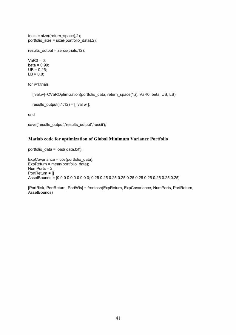
41

trials = size((return_space),2); portfolio_size = size((portfolio_data),2); results_output = zeros(trials,12); VaR0 = 0; beta = 0.99; UB = 0.25; LB = 0.0; for i=1:trials [fval,w]=CVaROptimization(portfolio_data, return_space(1,i), VaR0, beta, UB, LB); results_output(i,1:12) = [ fval w ]; end save('results_output','results_output','-ascii'); Matlab code for optimization of Global Minimum Variance Portfolio portfolio_data = load('data.txt'); ExpCovariance = cov(portfolio_data); ExpReturn = mean(portfolio_data); NumPorts = 2 PortReturn = [] AssetBounds = [0 0 0 0 0 0 0 0 0 0; 0.25 0.25 0.25 0.25 0.25 0.25 0.25 0.25 0.25 0.25] [PortRisk, PortReturn, PortWts] = frontcon(ExpReturn, ExpCovariance, NumPorts, PortReturn, AssetBounds)