LUNA:Analgorithmfor generatingdynamic planet-moon · PDF fileLUNA:Atransitalgorithmforexomoons...

arX

iv:1

105.

3499

v2 [

astr

o-ph

.EP]

23

Apr

201

2

Mon. Not. R. Astron. Soc. 000, 1–?? (2011) Printed 25 April 2012 (MN LATEX style file v2.2)

LUNA: An algorithm for generating dynamic planet-moon

transits

David M. Kipping1,2⋆⋆1Harvard-Smithsonian Center for Astrophysics, Garden St., Cambridge, MA 02138, USA2University College London, Dept. of Physics & Astronomy, Gower St., London, WC1E 6BT, UK

Accepted 2011 May 16. Received 2011 May 11; in original form 2011 February 26

ABSTRACT

It has been previously shown that moons of extrasolar planets may be detectablewith the Kepler Mission, for moon masses above ∼ 0.2M⊕ (Kipping et al. 2009c).Transit timing effects have been formerly identified as a potent tool to this end, ex-ploiting the dynamics of the system. In this work, we explore the simulation of transitlight curves of a planet plus a single moon including not only the transit timing effectsbut also the light curve signal of the moon itself. We introduce our new algorithm,LUNA, which produces transit light curves for both bodies, analytically accounting forshadow overlaps, stellar limb darkening and planet-moon dynamical motion. By build-ing the dynamics into the core of LUNA, the routine automatically accounts for transittiming/duration variations and ingress/egress asymmetries for not only the planet,but also the moon.We then generate some artificial data for two feasibly detectable hypothetical systemsof interest: a i) prograde and ii) retrograde Earth-like moon around a habitable-zoneNeptune for a M-dwarf system. We fit the hypothetical systems using LUNA and demon-strate the feasibility of detecting these cases with Kepler photometry.

Key words: techniques: photometric — planets and satellites: general — planetarysystems — eclipses — methods: analytical

1 INTRODUCTION

In recent years, the possibility of detecting the moons ofextrasolar planets, so-called “exomoons”, has received in-creased attention (Sartoretti & Schneider 1999; Han & Han2002; Szabo et al. 2006; Simon et al. 2009; Lewis et al. 2008;Kipping 2009a,b; Sato & Asada 2009; Kipping 2010b). Ex-trasolar moons may be frequent, temperate abodes for lifeand a determination of their prevalence would mould ourunderstanding of the abundance of life in the Universe. Al-though many techniques have been proposed, it is the tran-sit method which seems to offer the greatest potential to de-tect habitable-zone moons in the near-future (Kipping et al.2009c).

In general, there are two ways in which a moon canbe identified using transits. The first of these is the moon’sown transit light curve (Sartoretti & Schneider 1999) andthe second is the family of techniques known as “transittiming effects”. This includes both transit timing variations(TTV) (Sartoretti & Schneider 1999) and transit durationvariations (TDV). Further, TDV has two different compo-

⋆ E-mail: [email protected]

nents; one due to velocity variations (TDV-V) (Kipping2009a) and one due to transit impact parameter variations(TDV-TIP) (Kipping 2009b). TTV and TDV-TIP are bothdue to the position of the planet varying in response to themoon’s presence (positional wobble). In contrast, TDV-V isdue to velocity variation of the host planet in response to themoon’s presence (velocity wobble). Combining all of theseeffects allows for a unique solution (see Kipping 2009b fordetails) for the moon-to-planet mass ratio and exomoon pe-riod (and therefore orbital semi-major axis through Kepler’sThird Law).

To perform the observations, highly precise, contin-uous photometry is required and the Kepler Mission isthought to be the best instrument currently available toconduct such a search (Kipping et al. 2009c). So far, twosearches for exomoons have been conducted using the Ke-pler photometry, utilizing the transit timing techniques onKepler-4b through 8b (Kipping & Bakos 2011a) and TrES-2b (Kipping & Bakos 2011b). Despite null-results (whichwas expected as all of these planets are hot-Jupiters), thestudies indicate sensitivity into the sub-Earth mass regime,as predicted by Kipping et al. (2009c). The transit timingequations are all built around the premise of a constant

http://arxiv.org/abs/1105.3499v2

2 David M. Kipping

planet-star separation and constant planetary velocity dur-ing the timescale of the transit. Whilst this is generally agood approximation except for moons on very short peri-ods, there is an obvious desideratum to make the expressionsdynamic.

A possible problem with the current technique is that ifthe moon’s light curve is detectable directly, then not onlyis this an extra piece of data we are ignoring but also itcould fundamentally invalidate many of the transit timingmethods. The ideal solution would be to simulate both theplanet and moon transit light curves, including limb darken-ing which is critical for Kepler. In addition, these light curvescould be computed with the TTV and TDV effects inher-ently built into the model in a dynamic way. Not only wouldthis improve upon the static approximations made in theTTV/TDV equations, but it would also bring in TTV/TDVof the moon itself.

Before constructing such an algorithm, one must keepthe purpose of such a routine in mind. This algorithm willbe used to search for exomoons which will be done by fittinglight curves with the new algorithm. Given the large numberof free parameters and inevitable intricate inter-parameterdependencies, a Monte Carlo based method seems required.Since such methods are inherently computationally expen-sive making often millions of calls to the simulation rou-tine, then it is clear that any algorithm we design must bevery fast to execute. This essentially excludes methods basedupon pixelating the star or other numerical methods. Theclear requirement then, is a completely analytic algorithm.The list of requirements are:

Analytic (absolutely no numerical components) Dynamic (inherently accounts for all timing effects) Limb darkening incorporated (including non-linear

laws) All orbital elements accounted for (e.g. eccentricity, lon-

gitude of the ascending node, etc)

In summary, such an approach would not only offermany advantages over the previous timing methods, butwould also be highly practical for conducting a batch-stylesearch for exomoons in archival data. In this paper, we in-troduce the fundamental equations needed to construct thisalgorithm, known as LUNA, and apply it in some hypotheticalexamples.

In §2, we describe the framework for computing thetransit light curves of a planet with a moon and outline theassumptions made. Accompanying details on the model usedfor the sky-projected motions of the planet and moon can befound in the Appendix (§A). In §3, we provide expressionsfor the eclipsing area of the moon in front of the star in all27 possible principal configurations. In §4, example transitslight curves are generated and re-fitted for habitable-zoneexomoons detectable with Kepler -class photometry. Finally,we discuss comparison to previous methods proposed in theliterature and provide concluding remarks in §5.

2 LIGHT CURVE GENERATION

2.1 Converting Time to True Anomaly

To generate a light curve, the relative positions of the star,planet and moon must be calculated at every time stamp in

the photometric data set in question. In particular, one re-quires the sky-projected separation between the planet andstar, SP∗, the moon and the star, SS∗ and the planet and themoon, SPS . We direct the reader to the Appendix (§A) fordetails on the derivation of the expressions for these terms,where we employ an analytic approximation for the three-body problem which we dub as the nested two-body model(Kipping 2010b). The coordinate system employed through-out is also defined in the Appendix (§A). It can be shownthat these three S terms are a function of fB∗ and fSB whichmay be written, in general, as a function of time alone. Notethat we define fB∗ as the true anomaly of the planet-moonbarycentre around the star and fSB as the true anomalyof the satellite around the planet-moon barycentre. There-fore, a necessary prerequisite is to convert time stamps totrue anomalies. Let us begin with considering the standardpractice for a planet by itself.

2.1.1 The Planet-Only Case

The planet-only case is a very familiar one. However, wewill cover the conversion of time to true anomaly carefully.Writing out the steps explicity will allow us to identify thenecessary procedure for the more complicated planet-mooncase we will soon face.

Typically, we have a time series running from an initialtime stamp of t1 up to tN (where N is the total numberof measurements) with the time of transit minimum occur-ring at τ . Our first task is to convert the time array intoan f array. To accomplish this we must define a referencepoint in time at which the true anomaly is known. Whilstwe are free to use any reference point we so desire, a typ-ical choice is the time of transit minimum, τ . In the ex-ample above, this choice it will change our array to runfrom t′1(= t1 − τ ) → t′N (= tN − τ ) with the transit cen-tred at time t′ = 0. The true anomaly at the time of transitminimum can be found by solving dS/df = 0 for f . Foreven a planet-only case, this is non-trivial and leads to a bi-quartic equation (Kipping 2008). The solution may be foundby a series expansion about the point of inferior conjunctionf(t = τ ) = π/2− ω + η, where η represents a perturbationterm, which is given up to 6th-order in Kipping (2011).

The third and final step is the application of Kepler’sEquation. With the reference true anomaly known, this isconverted to a reference mean anomaly via the usual rela-tions (Murray & Dermott 1999). Then, the mean anomaliesat all times may be calculated since this parameter scales lin-early with time. Finally, the mean anomalies are convertedinto true anomalies using Kepler’s Equation.

So to summarize we have three steps: i) subtract thetime of transit minimum from all times ii) define the ref-erence anomaly as the time of transit minimum iii) assignmean anomalies for all times, which are then converted totrue anomalies using Kepler’s Equation.

For data spanning multiple transits, the reference timeshould be close to the weighted mean transit number. Thisselection typically minimizes the correlation between the or-bital period and reference time. In such a case, the range ofallowed values for the fitting routine to explore vary fromτ = (τguess − P/2) → (τguess + P/2). Moving outside of thisrange would cause the fitting routine to assign a differenttransit epoch as the reference transit instead.

LUNA: A transit algorithm for exomoons 3

2.1.2 The Planet-Moon Case

Now consider a planet with a moon. The barycentre of theplanet-moon system essentially behaves in the same waywhich was used to describe the planet-only case. The ob-served time of transit minimum of the planet is displacedfrom a linear ephemeris by a small time δt, due to transittiming variations (Kipping 2009a). However, the barycentrebehaves identically to before and still passes the star at aminimum when fB∗ = (π/2− ωB∗ + η). Therefore, there isno need to change anything here except that it is understoodthat the τ value we fit for is not the time of transit mini-mum of the planet but the time of transit minimum of theplanet-moon barycentre across the star, and thus we denoteit as τB∗.

For the moon, an analogous logic may be followed.There must exist a second time shift, τSB, to account for thephasing between the moon in its orbit around the barycen-tre. It also seems clear that this phase time has a range ofPSB (orbital period of the moon around the barycentre), inanalogy to the τB∗ case. Let us imagine we have subtractedτB∗ from all of our times so are left with times running from,say, t′1 → t′N . The obvious deduction is that we must nowsubtract a value τSB to get to a new time frame t′′, just aswe did for τB∗.

A natural choice for τSB is the instant whendSSB/dfSB = 0. In analogy to the previous case, this occursat fSB = π/2− ωSB + ηSB , where ηSB is the perturbationterm. Because this parameter is a phasing term, we preferto use φSB = (2πτSB)/PSB as a definition, to decrease thecorrelations with the orbital period.

2.2 Retrograde Orbits

A unique problem with LUNA is that exomoons can be eitherprograde or retrograde. Whilst for planets this is also true,it actually makes no difference to the transit light curve (al-though the Rossiter-McLaughlin phenomenon is affected).However, for a moon the sense of motion is distinguishablevia the TTV and TDV effects (Kipping 2009b), meaning itdoes affect the transits and so cannot be neglected.

We tackle this by treating retrograde moons as havingπ < iSB < 2π and prograde moons as having 0 < iSB < π.It is shown in Kipping (2011) that this definition producesthe correct retrograde behaviour for the selected coordinatesystem1.

We point out that the asymmetry between progradeand retrograde moons is small. The source of the asymmetrycomes from the relative phase difference between the TDV-V and TDV-TIP effects, which is 0 for prograde moons andπ for retrograde (Kipping 2009b). Therefore, the determina-tion of the sense of orbital motion is only generally possibleif both TDV-V and TDV-TIP effects are observable.

2.3 Small-Moon Approximation

From a naive perspective, one might start by consideringthat the transit light curve of a planet and a moon can be

1 Note that the longitude of the ascending node of the moonin its orbit around the planet-moon barycentre has the range0 6 ΩSB < 2π

computed by calculating the light curve of both separatelyand then simply adding the signals together. However, thereexists numerous scenarios where this would break down. Forexample, the moon could be eclipsing the star but fully in-side the planetary disc and thus the change in flux causedby the moon would be zero.

To overcome this, we start by generating the planetarylight curve in the normal way. This can be done using theMandel & Agol (2002) routine with any limb darkening lawwe wish and not making any size approximations. Havingcomputed this curve, we need to add on the contributionfrom the moon. What really matters is what part of themoon is “actively” transiting the star. We define this asthe area of the moon which overlaps the star but does notoverlap the planet. If we can find this area, then we couldcompute a light curve for a planet + moon without any limbdarkening effects immediately, which is a necessary first step.The subject of the moon’s actively transiting area will bederived later in §3.

For now, let us assume we know what this area is andcontinue to think about how the limb darkened light curve ofthe actively transiting moon can be computed. In general, weare interested in achieving two things i) focussing on moonsrather than, say, binary-planets2 ii) actually detecting suchsignals. The first of these means we are dealing with smallobjects such that s . 0.1 in all cases and most likely s . 0.01in most cases (where s is the ratio of the satellite-to-starradii). The second point means that we need to be ableto perform fits of transit light curves including all of theplanet and moon properties. The inevitably large amount ofparameter space necessitates computationally efficient andexpedient algorithms. Putting these two arguments togetherindicates that the best way forward is to employ the small-planet approximation case used in Mandel & Agol (2002).This will ensure accurate modelling of the limb darkeningbut very fast algorithms.

We stress that the planet is still modelled using thefull equations since the host planet could be a Jupiter sizedobject, yielding p > 0.1 (where p is the ratio of the planet-to-star radii). Therefore, we assume the moon is small and theplanet is not. One limitation of this assumption is “binary-Jupiters”. If we have a binary-planet system for which thesmaller body satisfies s > 0.1 then the algorithm we develophere will be limited in accuracy. However, the current focusof LUNA is solely to detect small bodies.

2.4 Limb Darkened Light Curve for the Actively

Transiting Lunar Component

2.4.1 Uniform source

Let us assume that the component of the moon’s area whichactively transits the star is known and equals AS,transit. Be-fore we can compute the resulting limb darkened light curvefrom this component, we must first consider the case for auniform source.

We start by assuming the actively transiting componentof the moon is equal to that which would transit in the ab-sence of a planet. In other words, we here ignore the planet

2 Although we intend to extend LUNA to binary-planets in future-work.

4 David M. Kipping

and will re-introduce it later. We follow the methodology ofMandel & Agol (2002), where the ratio of obscured to unob-scured flux is given as F e

S(s, SS∗) = 1−λeS(s, SS∗) (replacing

the appropriate symbols for the exomoon case):

λeS(s, SS∗) =

0 1 + s < SS∗

1π

[

s2κ0 + κ1 − κ2

]

|1− s| < SS∗ 6 1 + ss2 SS∗ 6 1− s1 SS∗ 6 s− 1,

(1)where κ1 = cos−1[(1 − s2 + S2

S∗)/2SS∗], κ0 = cos−1[(s2 +S2S∗ − 1)/2sSS∗] and κ2 = 0.5

√

4S2S∗

− (1 + S2S∗

− s2)2.The most interesting case is clearly (1 − s) 6 SS∗ 6

(1 + s), where only a portion of the moon transits the star.The area of the moon which transits the star may be denotedas αS∗ where the subscript indicates S is transiting ∗.

In this case, λeS = αS∗/π, but α really generally de-

scribes the area of intersection between any two circles. Weprefer to generalize the equations at this stage, which willprove useful later. Therefore, the area of intersection causedby object of radius r transiting object of radius R, withseparation S, is:

α(R, r, S) = r2κ0(R, r, S) +R2κ1(R, r, S)− κ2(R, r, S)

(2)

κ0(R, r, S) = arccos[S2 + r2 −R2

2Sr

]

(3)

κ1(R, r, S) = arccos[S2 +R2 − r2

2SR

]

(4)

κ2(R, r, S) =

√

4S2R2 − (R2 + S2 − r2)2

4(5)

Let us now re-introduce the planet. The consequencesare that in various circumstances the portion of the moon’sshadow which actively transits the star is diminished due tooverlap between the planet and the moon. We will discussthe derivation of the actively transiting lunar area in §3, butfor now it is sufficient to say that for a uniform source theloss of light due to the lunar component is:

F eS(s, SS∗) = 1− AS,transit

π(6)

As an example, in the case of no overlap between theplanet and the moon, but the moon fully inside the stellardisc, AS,transit = πs2 and thus we recover the expected formshown in Equation 1.

2.4.2 List of Cases

Looking at the equations for a uniform source (Equation 1),one may identify three distinct cases: i) moon fully outsidethe stellar disc ii) moon partially inside the stellar disc iii)moon fully inside the stellar disc. The first of these is triv-ial; there is no transit occurring. The third is also trivial fora uniform source but not so for a limb darkened one. Forreasons which become clearer later, it is necessary to sepa-rate ii) into two different cases dependent upon whether themoon overlaps the stellar centre or not (cases III and IX inthe original Mandel & Agol (2002) assignment). To summa-

Table 1. List of cases identified by Mandel & Agol (2002). Weuse the same case notation in this work, but modifying them toemphasise the focus on moons.

Case Condition Area of star which is eclipsed

I 1 + s < SS∗ < ∞ 0II 1− s < SS∗ < 1 + s αS∗

III s < SS∗ < 1− s πs2

IX 0 < SS∗ < s πs2

rize the different cases of interest, we direct the reader toTable 1.

2.4.3 Case III

Under the assumption of a small ratio-of-radii (s ≪ 1) onemay assume the surface brightness of the star is constantunder the disc of the transiting body (Mandel & Agol 2002).We will here assume non-linear limb darkening of the formI(r) = 1 −∑4

n=1cn(1 − µn/2), where I(r) represents the

radial intensity distribution from the star with I(0) = 1, µ =cos θ =

√1− r2 and r is the normalized radial coordinate

on the disc of the star. The non-linear limb darkening law(Claret 2000) is chosen as it may be easily used to computelower order limb darkening laws, specifically quadratic andlinear laws.

Let us draw an annulus inside the star with width 2s atradius SS∗ to represent this surface. We begin by consideringcase III, where the body is fully inside the star but does notcover the stellar centre (i.e. s < SS∗ < 1− s). We have:


Ftotal =

∫ 1

0

2rI(r) dr

= 1−4∑

n=1

ncnn+ 4

(7)

F IIIS,annulus(SS∗, s) =

∫ SS∗+s

SS∗−s

2rI(r) dr

=4

5c1

[

s2(

4√1− bm − 4

√1− am

)

+(

S2S∗ − 1

)

(

4√1− bm − 4

√1− am

)

+ sSS∗

(

2 4√1− am + 2 4

√1− bm − 5

)

]

+2

21

[

7c2[

(s2(√

1− bm −√1− am

)

+(

S2S∗ − 1

)

(√1− bm −

√1− am

)

+ 2sSS∗

(√1− am +

√1− bm − 3

) ]

− 6[

c3(

s2(

(1− am)3/4 − (1− bm)3/4)

+ S2S∗

(

(1− am)3/4 − (1− bm)3/4)

+ sSS∗

(

−2 (1− am)3/4 − 2(1− bm)3/4 + 7)

− (1− am)3/4 + (1− bm)3/4)

+ 7sSS∗

(

c4(

s2 + S2S∗

)

− 1)

]

]

(8)

where am = (SS∗ − s)2 and bm = (SS∗ + s)2 and the msubscript denotes this definition comes from Mandel & Agol(2002). A further simplification is possible by using amr =(1− am)1/4 and bmr = (1− bm)1/4.

F IIIS,annulus(SS∗, s) =

4

5

[

s2(bmr − amr) + (S2S∗ − 1)(bmr − amr)

+ 2sSS∗

(

− 5

2+ amr + bmr

)]

c1

+2

21

[

7(

s2(b2mr − a2mr) + (S2S∗ − 1)(b2mr − a2mr)

+ 2sSS∗(−3 + a2mr + b2mr))

c2

− 6

(

(

b3mr − a3mr + 2sSS∗(7

2− a3mr − b3mr)

+ s2(a3mr − b3mr) + S2S∗(a

3mr − b3mr)

)

c3

+ 7sSS∗(−1 + (s2 + S2S∗)c4)

)]

(9)

The final step is to acknowledge that the transitingbody does not transit an area equal to that of the annulus,but in general, a smaller area. Therefore, we must multiplythe flux from the annulus by a ratio-of-areas given by:

AIIIS =

AS,transit

AIIIS,annulus

(10)

=AS,transit

π[(SS∗ + s)2 − (SS∗ − s)2]

AIIIS =

AS,transit

π(bm − am)(11)

The final flux is given by:

F eS = 1−Ae

S

(F eS,annulus

Ftotal

)

(12)

2.4.4 Case IX

If the transiting body has an equatorial orbit, such thatSS∗ < s, the setup for case III is invalid since one of theintegration limits is negative and r is strictly defined to ber > 0. This gives us case IX:

F IXS,annulus =

∫ SS∗+s

0

2rI(r) dr

=4

5

[

1− bmr + (s+ SS∗)2(

− 5

4+ bmr

)

]

c1

+2

3

[

1− b2mr + (s+ SS∗)2(

− 3

2+ b2mr

)

]

c2

+1

14

[

14(s + SS∗)2 − 7(s+ SS∗)

4c4

+ 2(

4− 4b3mr + (s+ SS∗)2(−7 + 4b3mr)

)

c3

]

(13)

For the ratio of the annulus to actively-transiting-lunararea we have:

AIX =AS,transit

πbm(14)

2.4.5 Case II

The final case we need is case II. This is when the body isin the ingress/egress portion i.e. (1− s) < SS∗ < (1 + s). Inthis case the annulus flux is given by:

F IIS,annulus =

∫ 1

SS∗−s

2rI(r) dr

=1

5(−5 + 4amr)a

4mrc1

+am − 1

42

[

− 42 + (42− 28a2mr)c2 + 6(7− 4a3mr)c3

+ 21(1 + am)c4

]

(15)

The ratio of the annulus to actively-transiting-lunararea is:

6 David M. Kipping

AII =AS,transit

π(1− am)(16)

2.5 Summary

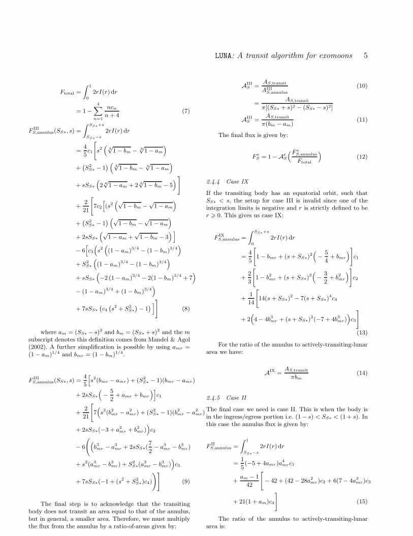
The light curve of the actively-transiting-lunar compo-nent has now been evaluated, but we have not yet de-rived AS,transit: the sky-projected area of this component.The planetary light curve is computed using the usualMandel & Agol (2002) routine, utilizing SP∗. The only re-maining task is therefore to find AS,transit, which we dealwith next in §3.

3 ACTIVELY TRANSITING LUNAR AREA

3.1 Principal Cases

The one-body case is described by one parameter, S, whichcan have three states. As we saw in §2, the light curve ofthe actively-transiting-lunar component can be generated ineach case by just knowing SS∗ and AS,transit, in the smallmoon approximation. In what follows, we always assumes2 < p2 < 1 where s = RS/R∗. It is therefore clear thatour task is to find AS,transit in all possible configurations i.e.the actively transiting area. This will enable us to computeAe in cases II, III and IX and thus produce limb darkenedtransit light curves for the moon.

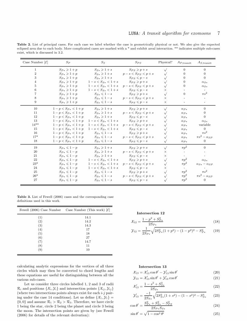
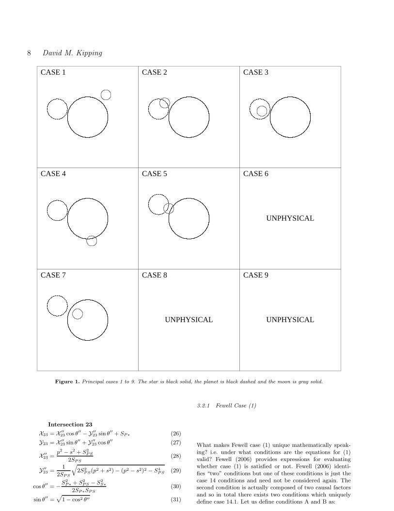
With three S values now in play (SP∗, SS∗ & SSP )more cases are possible than before. In total 33 = 27 prin-cipal cases exist, but many of these are unphysical underthe conditions that R > p > s (where R = 1) and thatSPS < |SP∗ − SS∗|. In Table 2, we list all the possible casesby permuting each S parameter into each of their respectivethree states. The cases which are unphysical are marked ac-cordingly. Figures 1, 2 & 3 illustrate example configurationsfor each principal case.

Table 2 shows that for some cases, the amount of lunararea actively transiting the star is dependent upon the posi-tion of the planet (these case are marked with a *). This isbecause the planet’s shadow overlaps with the lunar shadowand so the the moon cannot block out to its full potential.We label these cases as exhibiting “areal interaction”.

3.1.1 Case 26

We start by considering the simplest of the areal interac-tion cases, case 26 (see Figure 3). We denote this as E26 inmathematical notation (and likewise for the other case num-bers). E is chosen in analogy to the case notation e used byMandel & Agol (2002). For case 26, the planet and moonare both completely inside the stellar disc but are inter-acting with each other. This is very similar to the case IIsituation for a one-body transit where the star has becomethe planet and the transiting-body has become the moon.So R, p, S → p, s, SPS. The area of the moon which leftactively transiting the star is given by AE26

S,transit = πs2−αSP .

3.1.2 Case 17

The next most complicated case is case 17. Here the planetis on the limb of the star and the moon is on the limb of theplanet, but completely within the star. It can be seen thatAE27

S,transit = AE26S,transit = πs2−αSP and thus we already have

the required equation in hand.

3.1.3 Case 23

The third most complicated case is when the planet is com-pletely inside the star but the moon sits on the planetarylimb and coincidentally the stellar limb. If the planet wasnot present, the moon would eclipse an area given by αS∗.

However, the planet is present, and it blocks out a por-tion of this area. Under the conditions of case 23, the over-lapping area between the planet and moon must always liecompletely within the stellar disc since the planet alwayslies completely within the stellar disc. It can be therefore beseen that the overlapping area, αSP , will always be less thanαS∗. Therefore, the final area which is actively transiting thestar from the moon alone is:

AE23S,transit = αS∗ − αSP (17)

3.2 The Sub-Cases of Case 14

Case 14 is the most complicated case to consider. Indeed,case 14 actually has multiple sub-cases which define the var-ious possible behaviours. Although similar to case 23, theplanet’s shadow now does not completely eclipse the starand so the overlapping area between the moon and planetalso does not necessarily have to lie completely within thestellar disc. As a consequence, multiple different states existand a singular expression is not possible for AS,transit.

The first key question is: how many sub-cases actuallyexist? The problem we are thinking of is that of three cir-cles interacting to give an overlapping region, for which werequire the associated area. The problem of finding the areaof overlap between three circles was studied extensively inthe pioneering work of Fewell (2006). Indeed, an analytic so-lution for the overlap of three circles did not exist until 2006when Fewell presented the solution. Fewell (2006) identifiednine possible cases in total, which we label as Fewell case(1) → (9) and viewable in Figure 5 of Fewell (2006). To as-sign identities in our framework, we label the biggest circlethe star, the middle-sized circle the planet and the smallestcircle the moon in Figure 5 of Fewell (2006).

Going through the Fewell (2006) scenarios with our as-signed identities, the first thing we notice is that only fourof the Fewell (2006) cases remain consistent with the case14 conditions, the others are much simpler scenarios whichwe dealt with earlier as the principal cases. In Table 3, weshow the corresponding case numbers to the Fewell (2006)cases for completion.

The Fewell (2006) solution for the area of common over-lap between three circles is based upon a formula for thecircular triangle, which uses the chord lengths and radii ofthe three circles involved. Only in Fewell case (1) does a cir-cular triangle actually exist and this is the focus of Fewell(2006). However, Fewell (2006) performs the derivation by


Table 2. List of principal cases. For each case we label whether the case is geometrically physical or not. We also give the expectedeclipsed area due to each body. More complicated cases are marked with a * and exhibit areal interaction. ** indicates multiple sub-casesexist, which is discussed in 3.2.

Case Number [E] SP SS SPS Physical? AP,transit AS,transit

1 SP∗ > 1 + p SS∗ > 1 + s SPS > p+ s√

0 02 SP∗ > 1 + p SS∗ > 1 + s p− s < SPS < p+ s

√0 0

3 SP∗ > 1 + p SS∗ > 1 + s SPS 6 p− s√

0 04 SP∗ > 1 + p 1− s < SS∗ < 1 + s SPS > p+ s

√0 αS∗

5 SP∗ > 1 + p 1− s < SS∗ < 1 + s p− s < SPS < p+ s√

0 αS∗

6 SP∗ > 1 + p 1− s < SS∗ < 1 + s SPS 6 p− s × - -7 SP∗ > 1 + p SS∗ 6 1− s SPS > p+ s

√0 πs2

8 SP∗ > 1 + p SS∗ 6 1− s p− s < SPS < p+ s × - -9 SP∗ > 1 + p SS∗ 6 1− s SPS 6 p− s × - -

10 1− p < SP∗ < 1 + p SS∗ > 1 + s SPS > p+ s√

αP∗ 011 1− p < SP∗ < 1 + p SS∗ > 1 + s p− s < SPS < p+ s

√αP∗ 0

12 1− p < SP∗ < 1 + p SS∗ > 1 + s SPS 6 p− s√

αP∗ 013 1− p < SP∗ < 1 + p 1− s < SS∗ < 1 + s SPS > p+ s

√αP∗ αS∗

14** 1− p < SP∗ < 1 + p 1− s < SS∗ < 1 + s p− s < SPS < p+ s√

αP∗ variable15 1− p < SP∗ < 1 + p 1− s < SS∗ < 1 + s SPS 6 p− s

√αP∗ 0

16 1− p < SP∗ < 1 + p SS∗ 6 1− s SPS > p+ s√

αP∗ πs2

17* 1− p < SP∗ < 1 + p SS∗ 6 1− s p− s < SPS < p+ s√

αP∗ πs2 − αSP

18 1− p < SP∗ < 1 + p SS∗ 6 1− s SPS 6 p− s√

αP∗ 0

19 SP∗ 6 1− p SS∗ > 1 + s SPS > p+ s√

πp2 020 SP∗ 6 1− p SS∗ > 1 + s p− s < SPS < p+ s × - -21 SP∗ 6 1− p SS∗ > 1 + s SPS 6 p− s × - -22 SP∗ 6 1− p 1− s < SS∗ < 1 + s SPS > p+ s

√πp2 αS∗

23* SP∗ 6 1− p 1− s < SS∗ < 1 + s p− s < SPS < p+ s√

πp2 αS∗ − αSP

24 SP∗ 6 1− p 1− s < SS∗ < 1 + s SPS 6 p− s × - -25 SP∗ 6 1− p SS∗ 6 1− s SPS > p+ s

√πp2 πs2

26* SP∗ 6 1− p SS∗ 6 1− s p− s < SPS < p+ s√

πp2 πs2 − αSP

27 SP∗ 6 1− p SS∗ 6 1− s SPS 6 p− s√

πp2 0

Table 3. List of Fewell (2006) cases and the corresponding casedefinitions used in this work.

Fewell (2006) Case Number Case Number (This work) [E]

(1) 14.1(2) 14.2(3) 14.3(4) 17(5) 18(6) 27(7) 14.7(8) 11(9) 10

calculating analytic expressions for the vertices of all threecircles which may then be converted to chord lengths andthese equations are useful for distinguishing between all thevarious sub-cases.

Let us consider three circles labelled 1, 2 and 3 of radiiRi and positions Xi,Yi and intersection points Xij ,Yij(where two intersections points always exist for each i-j pair-ing under the case 14 conditions). Let us define X1,Y1 =0, 0 and assume R1 > R2 > R3. Therefore, we have circle1 being the star, circle 2 being the planet and circle 3 beingthe moon. The intersection points are given by (see Fewell(2006) for details of the relevant derivation):

Intersection 12

X12 =1− p2 + S2

P∗

2SP∗

(18)

Y12 =1

2SP∗

√

2S2P∗

(1 + p2)− (1− p2)2 − S4P∗

(19)

Intersection 13

X13 = X ′13 cos θ

′ −Y ′13 sin θ

′ (20)

Y13 = X ′13 sin θ

′ + Y ′13 cos θ

′ (21)

X ′13 =

1− s2 + S2S∗

2SS∗

(22)

Y ′13 =

−1

2SS∗

√

2S2S∗

(1 + s2)− (1− s2)2 − S4S∗

(23)

cos θ′ =S2P∗ + S2

S∗ − S2PS

2SP∗SS∗

(24)

sin θ′ =√

1− cos2 θ′ (25)

8 David M. Kipping

CASE 1 CASE 2 CASE 3

CASE 4 CASE 5

UNPHYSICAL

CASE 6

CASE 7

UNPHYSICAL

CASE 8

UNPHYSICAL

CASE 9

Figure 1. Principal cases 1 to 9. The star is black solid, the planet is black dashed and the moon is gray solid.

Intersection 23

X23 = X ′′23 cos θ

′′ −Y ′′23 sin θ

′′ + SP∗ (26)

Y23 = X ′′23 sin θ

′′ + Y ′′23 cos θ

′′ (27)

X ′′23 =

p2 − s2 + S2PS

2SPS(28)

Y ′′23 =

1

2SPS

√

2S2PS(p

2 + s2)− (p2 − s2)2 − S4PS (29)

cos θ′′ = −S2P∗ + S2

PS − S2S∗

2SP∗SPS(30)

sin θ′′ =√

1− cos2 θ′′ (31)

3.2.1 Fewell Case (1)

What makes Fewell case (1) unique mathematically speak-ing? i.e. under what conditions are the equations for (1)valid? Fewell (2006) provides expressions for evaluatingwhether case (1) is satisfied or not. Fewell (2006) identi-fies “two” conditions but one of these conditions is just thecase 14 conditions and need not be considered again. Thesecond condition is actually composed of two causal factorsand so in total there exists two conditions which uniquelydefine case 14.1. Let us define conditions A and B as:



CASE 13

MULTIPLE SUB-CASES

CASE 14 CASE 15



Condition A

(X12 − SS∗ cos θ′)2 + (Y12 − SS∗ sin θ

′)2 < s2 (32)

Condition B

(X12 − SS∗ cos θ′)2 + (Y12 + SS∗ sin θ

′)2 < s2 (33)

In order to have case 14.1, we require that conditionA is satisfied and condition B is anti-satisfied (we call thiscondition B). The area αtransit may be found by evaluatingthe circular triangle, principally defined by the chord lengthsand radii. In fact, two sub-sub-cases exist here for 14.1 whichwe label as 14.1a and 14.1b. 14.1a is the case where less than

half the circle is involved and 14.1b occurs when more thanhalf the circle is involved. The two cases are distinguishedby evaluating the following:

Condition C

SS∗ sin θ′ > Y13 +

Y23 − Y13

X23 − X13

(SS∗ cos θ′ −X13) (34)

If the above equation is true (condition C) then we havecase 14.1a and AE14.1a

overlap may be found using:

10 David M. Kipping

CASE 19

UNPHYSICAL

CASE 20

UNPHYSICAL

CASE 21

CASE 22 CASE 23

UNPHYSICAL

CASE 24



AE14.1aoverlap =

1

4

√

(c1 + c2 + c3)(c2 + c3 − c1)

×√

(c1 + c3 − c2)(c1 + c2 − c3)

+

3∑

k=1

(

R2k arcsin

ck

2Rk− ck

4

√

4R2k − c

2k

)

(35)

c2k = (Xik − Xjk)

2 + (Yik − Yjk)2 (36)

Otherwise (condition C), for case 14.1b, we must use:

AE14.1boverlap =

1

4

√

(c1 + c2 + c3)(c2 + c3 − c1)

×√

(c1 + c3 − c2)(c1 + c2 − c3)

+3∑

k=1

(

R2k arcsin

ck

2Rk

)

− c1

4

√

4R21 − c

21 −

c2

4

√

4R22 − c

22 +

c3

4

√

4R23 − c

23

(37)

The actively transiting area of the moon is now givenby: AE14.1x

S,transit = αS∗ − AE14.1xoverlap. In the above equations, it

should be noted that ck represents the chord lengths.



Fewell (2006) does not discuss in any detail how to computethe area of overlap for Fewell case (2), but this is simplerthan Fewell case (1). In Fewell case (1) we had a circulartriangle, whereas case (2) presents a circular quadrilateral.Before we consider the various scenarios, let us define underwhat conditions Fewell case (2) is satisfied.

For Fewell case (2), the constraint is that the two inter-section points of circles 1 and 2 both lie outside of circle 3(this narrows it down to Fewell case (2) or (7)). Thereforewe must satisfy conditions A and B.

Next, the intersection points of circles 1 and 3 must lieinside circle 2 (this distinguishes it from Fewell case (7)).Assuming case 14, condition A and condition B, it is notphysically possible to have a solution where one of theseintersection points lies inside and the other outside of circle2. It is, however, possible to have both outside, which givesrise to Fewell case (7). Because of this fact, we only need touse one of the intersection points to define condition D:

Condition D

(X13 − SP∗)2 + Y2

13 < p2 (38)

But, even this is not enough for a unique solution. InFewell case (2) of Figure 5 of Fewell (2006), one could imag-ine mirroring the moon along the line connecting the twomoon-star intersection points. This would still satisfy all ofthe above conditions but now no part of the moon is activelytransiting. The nominal case, as shown in Figure 5 of Fewell(2006), is labelled as 14.2a (shown in Figure 4), whereas thealternative case is 14.2b. Therefore, we define condition E,which if satisfied gives case 14.2a and if anti-satisfied givescase 14.2b:

Condition E

(SS∗ − s) < (SP∗ − p) (39)

Case 14.2a has AE14.2aS,transit = πs2 − αSP , otherwise for

14.2b we have AE14.2bS,transit = 0.


To meet Fewell case (3), both intersection points of 1 and 2must lie inside circle 3 i.e. condition A and B. Sub-case 14.3contains two possible sub-sub-cases; 14.3a and 14.3b. Thesecond sub-sub-case was identified quite late in our analysisand noticed during testing and debugging.

The two cases are differentiated by whether the planet’scentre is inside or outside the stellar disc. If outside, thenwe have case 14.3a, which satisifes condition F.

Condition F

SP∗ > 1 (40)

In this case, 14.3a, AE14.3aS,transit = αS∗ − αP∗. For case

14.3b, the planet is inside and we have AE14.3bS,transit = πp2 −

αSP − αP∗ + αS∗.

Table 4. List of sub-cases and conditions. A bar indicates thecondition is anti-satisfied.

Sub-Case Conditions Satisfied AS,transit

14.1a A; B; C αS∗ − AE14.1aoverlap

14.1b A; B; C αS∗ − AE14.1boverlap

14.2a A; B; D; E πs2 − αSP

14.2b A; B; D; E 014.3a A; B; F αS∗ − αP∗

14.3b A; B; F πp2 − αP∗ − αSP + αS∗

14.7a A; B; D; G αS∗

14.7b A; B; D; G αS∗ − αSP


For Fewell case (7), we must satisfy conditions A and B, asdid Fewell case (2). The final condition for Fewell case (7)is simply the opposite of condition D, i.e. condition D.

However, this is insufficient to give a unique solution.The standard Fewell case (7) has no interaction betweenthe planet and moon within the stellar disc but this is nota condition, merely an artifact of the figure’s construction.It is possible that the intersection points of 1 and 2 liesoutside circle 3, and the intersection points of 1 and 3 liesoutside 2, but still two distinct cases exist. These two sub-sub-cases are that if the intersection of 2 and 3 lies within1, then areal interactions must be occurring. We label thiscase 14.7b. Case 14.7a is that the circles do not interact.

This first case occurs when both intersection points of2 and 3 lie outside of circle 1. It is not possible to have oneinside and one outside under the previous conditions so farmet. Thus we have condition G, which if satisfied yields case14.7b and if anti-satisfied gives 14.7a.

Condition G

X 223 + Y2

23 < 1 (41)

Accordingly, AE14.7aS,transit = αS∗. Otherwise the planet-

moon intersections occur within the star and thereby neces-sitating a degree of interaction (case 14.7b, satisfying con-dition G), for which AE14.7b

S,transit = αS∗ − αSP .

3.2.5 Summary of Sub-Cases

This completes every possible scenario for three circles in-teracting. The sub-case conditions are summarized in Ta-ble 4 and illustrated example configurations are shown inFigure 4. We have calculated the area of overlap in everycase in an analytic manner. This will allow for extremelyexpedient computation of the light curve from a planet plusmoon.

Due to the plethora of cases, sub-cases and even sub-sub-cases, a large amount of testing of the LUNA algorithmhas been executed. This was done by trying various systemconfigurations and ensuring no gaps existed in the case con-ditions or unusual light curve features were produced by thealgorithm. It was during this stage which we identified thatsub-case 14.3 actually had two sub-sub-cases in the form of14.3a and 14.3b.

12 David M. Kipping

CASE 14.1 a CASE 14.1 b CASE 14.2 a

CASE 14.2 b CASE 14.3 a CASE 14.3 b

CASE 14.7 a CASE 14.7 b

Figure 4. Sub-cases of case 14. The subscript numbers (1,2,3,7) originate from the system employed by Fewell (2006). The extra caseconditions (a,b) come from additional complexity within each sub-case yet consistent within the original case definitions of Fewell (2006).The star is black solid, the planet is black dashed and the moon is gray solid. Relative sizes selected purely for depiction purposes.

3.3 Flow Decision Diagram

With all the conditions stated, it is useful to construct a flowdiagram of the decision route which LUNA should take. Thisflow diagram should be designed to minimize the number ofcalculations LUNA has to perform. We have conditions A toG for the sub-cases and three additional conditions from theprincipal cases, so the maximum number of decisions in anychain should be 10. Ideally, most decision routes will involvefewer than 10 decisions.

3.3.1 Decision 1

The best-place to start is with the principal cases. The com-putation of the transit light curve will always require a com-putation of SP∗, as it is assumed that the planet alwaystransits.

Since we always have to compute this term anyway, theeconomic way to proceed is to base a decision tree upon itsbehaviour. This essentially gives us a three way-split intothree decision trees: cases 1 through 9 (called “p-out”), 10through 19 (“p-part”) and 20 through 27 (“p-in”).


3.3.2 Decision 2

Having computed SP∗, should we compute SS∗ and SPS?In several cases, only one of these is required to calculatethe light curve. Consider, the p-out tree first (note that thesecond decision does not have to be the same in each tree).Since the planet is out of the stellar disc, areal interactionis impossible and thus SPS need never be computed. There-fore, the logical second decision for p-out is simply to eval-uate SS∗ and see which of the three possible circumstancesit is in.

For the p-in tree, there are two possible questions onecould pose. Remember, we wish to pose the question whichleads to the most efficient algorithm. First possible question:evaluate SS∗ and see which state it is in. Second possiblequestion: evaluate SSP and see which state it is in.

If we ask the second question, the in-case requires nofurther computations. However, the part and out cases bothrequire that we evaluate SS∗ to proceed.

If we ask the first question, the out case requires nofurther computation. However, the in and part cases requirewe calculate SSP . Therefore, the two approaches seem toyield equivalent levels of complexity. In general, if the moonis transiting, SS∗ will always be needed whereas SSP is onlyneeded if areal interaction occurs. Therefore, we prefer toask about SS∗ first.

Finally, for the p-part tree, case 14 is the mix which isby the far the most complicated case computationally. Wewish to choose a tree based upon minimizing our exposure tocase 14. SS∗ again makes a natural choice by the groupingsof the actively transiting area formulas.

3.3.3 Decision 3

Since decision 2 is always the same, decision 3 is simply toevaluate SSP and check its condition. There is no choice inthis.

3.3.4 Decision 14.1

If case 14 occurs, we have a new decision tree opening up dueto presence of sub-cases. The first decision is decision 14.1.Unlike the principal tree, each sub-case does not necessarilyinvolve a calculation of all the possible conditions. There-fore, some conditions crop up more frequently than others.If all the conditions took the same time to compute, then wewould prefer to compute those conditions which occur mostfrequently early on in our decision tree.

Conditions A and B clearly provide the backbone tothe decision tree and thus must be evaluated early on. Theirevaluation is ultimately unavoidable so should be done atthe start. Case 14.3 is unusual in that it can be identified assatisfying condition B only since all sub-cases anti-satisfy B.Condition B is therefore the obvious starting point in ourdecision tree. If verified, we have case 14.3 and if not wemove into decision 14.2.

3.3.5 Decision 14.2

Since conditions A and B are the backbone and B has beenevaluated, the next step is to evaluate A. If satisfied, we

have case 14.1. Anti-satisfaction means we have either 14.2or 14.7.

3.3.6 Decision 14.3

If we have 14.1, then decision 14.3 must be to evaluate con-dition C. If we have 14.2 or 14.7, then the discriminator iscondition D.

3.3.7 Decision 14.4

Not needed for 14.1 cases, but for Fewell cases (2) and (7)we must compute conditions E and G respectively.

3.3.8 Summary of decision tree

Figure 5 shows the decision process in a flow chart to sum-marize the approach of LUNA.

4 EXAMPLE TRANSIT LIGHT CURVES

4.1 Dealing with Inclination

Transit modellers will be familiar with the pot-holes in theroad presented when trying to fit transit light curves withthe physical parameters. To start with, inclination is almostalways in the range ∼85 to 90 degrees and fitting for iB∗

yields large correlations and lethargic routines. In practice,it is better to define the impact parameter of the transitchord across the star, bB∗.

bB∗ = (rB∗/R∗) cos iB∗ (42)

A similar strategy would seem advisable for moons andwe can define an analogous quantity:

bSB = (rSB/RP ) cos iSB (43)

It should be noted that bSB is only the impact param-eter in the reference frame of the moving barycentre andwill not be the observed impact parameter in the sky frame.Therefore, bSB can be greater than unity and yet the moonstill transits the star.

Another subtlety is that iSB = π/2 + δ would give adifferent light curve than iSB = π/2 − δ, but both wouldyield the same value for bSB (in contrast to the situa-tion for a planet by itself). To account for this asymme-try, negative impact parameters are perceived as yieldingiSB = π − cos−1[RP bSB/rSB]. Retrograde satellites withinclinations in the range π < iSB < 2π are adjusted in asecond step where if a logical flag for retrograde orbits isswitched on, π is added onto the inclination.

4.2 Fitting Parameter Set

A typical planetary parameter set would beτ, p2, (a/R∗), b. Due the strong correlation between(a/R∗) and b (Carter et al. 2008), it is preferable to switchone of these parameters for a less correlated term. A typicalchoice is T , the duration for the planet to move from itscentre overlapping the stellar limb to exiting under the

14 David M. Kipping

Figure 5. Flow chart showing the decision process of choosing which case we are in. The decision tree has been optimized to marginalizethe more CPU intensive computations until absolutely required. The principal cases are not shown but are easily seen in Table 2. Squareboxes indicate an evaluation of whatever is inside the box. Black arrows indicate a true statement and the dot-dashed gray arrowsindicate a false.


same condition. An inverse-mapping expression to go fromT to (a/R∗) is given in Kipping (2010a). Note that a Tequation for the moon is not possible since bSB > 1 ispermitted and thus T would be complex.

We now have the four fitted parametersτB∗, p

2, TB∗, bB∗ for the planet-moon barycentre.Additionally, we need the orbital period, PB∗, which maybe fitted for if multiple transits exist. Radial velocity orsecondary eclipse information may be used to expandthe parameter set to include eB∗ cosωB∗ and eB∗ sinωB∗.Finally, the out-of-transit flux, OOT, and the blendingfactor, B (which cannot be fitted for) should also beincluded. The quadratic limb darkening coefficients u1 andu2 give an additional two parameters bringing the totalto 11. RV data may also require additional terms such assemi-amplitude, K, velocity offset, γ, etc.

To include the exomoon, 9 new parameters are needed:φSB, (MS/MP ), s, (aSB/R∗), bSB, PSB, eSB cosωSB,eSB sin ωSB, ΩSB. In total, this means we have 20+RV pa-rameters. In practice, not all of these will be fitted for e.g.the blending factor.

4.3 Example Simulations & Fits

In the next three subsections (§4.4-4.6) we provide threesimulations generated by LUNA. The system configurationused in each case is discussed in the relevant subsections. Ineach case, we use a cadence of 1minute and add on Gaus-sian noise of 250 ppm, in-line with the properties of Kepler ’sshort-cadence photometry (Kipping & Bakos 2011b). Dataare produced surrounding ±0.5 days of τB∗ for N consecu-tive transit epochs.

These noised light curves are then fitted using aMetropolis-Hastings MCMC routine with 125,000 steps anda 20% burn-in to give 105 final points for building the pa-rameter posteriors. Jump-sizes are set to be equal to the 1-σ uncertainties (determined through preliminary runs) andthe final parameter values are given by the median of eachparameter with uncertainties of 34.15% quantiles either side.

For each case, we perform three fits with fixed assump-tions i) no moon is present i.e. s = 0 and MS/MP = 0 ii)the moon is prograde (i.e. iSB is bounded to be in the range0 < iSB 6 π) iii) the moon is retrograde (π < iSB 6 2π).In reality, only one case is genuine and the two other actto show how distinguishable each scenario really is. We al-ways assume a circular orbit for the moon and planet forsimplicity, which removes four parameters.

In all cases, we utilize a powerful trick pointed out inKipping (2010b). The detection of a planet-moon system al-lows one to determine the absolute mass and radius of thehost star through Kepler’s Third Law alone. Armed withthese parameters, the planetary and lunar physical dimen-sions may also be obtained, thus replacing the traditionalneed for invoking spectroscopy and stellar evolution mod-els. The only additional information one requires is the ra-dial velocity semi-amplitude induced by the planet-moonbarycentre, K. As the observational uncertainty on this pa-rameter scales with ∼ 1/

√NRV, where NRV is the number

of RV measurements, it can be determined to high precisionby simply repeating the radial velocity observations.

As shown in Kipping (2010b), the absolute dimen-sions of the star have scalings M∗ ∼ K3

∗ and R∗ ∼ K∗,

and so [σ(M∗)]2 ≃ [3σ(K∗)]

2 + [σ(M ′∗)]

2 and [σ(R∗)]2 ≃

[σ(K∗)]2 + [σ(R′

∗)]2, where the dashed terms denote the

value derived assuming no error on K∗. In an exampleshown later (see §4.5), K∗ = 6m/s and σ(M ′

∗)/M′∗ ≃ 15%

and σ(R′∗)/R

′∗ ≃ 6%. This example is a singular case but

nonetheless serves the purpose of illustrating a feasible situ-ation. In this example, the assumption that K∗ contributesnegligible error into the stellar mass determination is validfor σ(K∗)/K∗ .2.5% (∼ 0.15m/s) and for the stellar ra-dius σ(K∗)/K∗ .7.0% (∼ 0.4m/s). These RV precisions arecomparable to values being reported by those using high-precision facilities such as Keck and HARPS (Vogt et al.2010; Lovis et al. 2011). More generally, once an exomoonsystem is found, the uniqueness and importance of the sys-tem would certainly warrant the exploitation of such spec-trographic resources and so high levels of precision in K∗

can be expected.We therefore assume that the uncertainty onK∗ is much

less than the uncertainty on the photometrically determinedexomoon parameters in what follows. The inclusion of thedetermination of M∗ and R∗ using the Kipping (2010b)method will demonstrate the feasibility of the technique.

We note that s and MS/MP are positive definiteand thus always yield a non-zero result. To identify caseswhere this bias is creating a false-positive, we apply theLucy & Sweeney (1971) test. If s or MS/MP yield a false-alarm-probability below 5%, then we quote the MCMC re-sult as usual. Otherwise, we quote the 95% confidence upperlimit on those parameters.

4.4 HZ-Neptune with a Close, Prograde Moon

around an M2 Star

4.4.1 Simulation and Fitting

As a first example, we consider a Neptune-mass and radiusplanet in orbit an M2 star in the habitable-zone (K∗ =6.0ms−1). Using the stellar parameters from Cox (2000),we assign M∗ = 0.40M⊙ and R∗ = 0.50R⊙. We place theplanet in an orbital period of PB∗ = 46.0 days in a circularorbit with iB∗ = 90. Quadratic limb darkening coefficientswere generated using a Kurucz (2006) style atmosphere fol-lowing the methodology of Kipping & Bakos (2011b), givingu1 = 0.3542 and u2 = 0.3607. In total, we generate N = 6transit epochs spanning 0.85 years of continuous photome-try.

For the exomoon, we consider an Earth-mass and radiusmoon on a close, prograde orbit around the host planet. Wetherefore select aSB to be 5% of the Hill radius, correspond-ing to ≃ 2RP . Through Kepler’s Third Law, the orbitalperiod is PSB = 0.3142 days. Such a moon would be ex-periencing large tidal dissipation and may not necessarilypersist for Gyr, however, this is irrelevant for the purpose ofgenerating some example transit light curves. We choose toplace the moon in a slightly inclined orbit of iSB = 92.93,corresponding to bSB = −0.1. We also use ΩSB = 5 andassume a circular orbit. In the left panel of Figure 6, thesimulated light curve is shown, before any noise is added.

Due to the low impact parameter of the barycentre andthe high coplanarity, TDV-TIP effects will be small andthus a determination of the sense of orbital motion willbe highly challenging (see §2.2 for explanation). However,

16 David M. Kipping

coplanarity is a reasonable choice as highly inclined moonshave reduced Hill stability (Donnison 2010) and thus areless likely a-priori. The same argument is true for eccentricmoons (Domingos et al. 2006).

4.4.2 Results

As discussed in §4.3, we performed three fits for prograde,retrograde and no moon assumptions. A comparison of thefitted parameters for each assumption is presented in Ta-ble 5, including the χ2 and Bayesian Information Crite-rion (BIC) of the best-fits for each model. BIC (Schwarz1978; Liddle et al. 2007) is a tool for model selection whichseverely penalizes models for including more degrees of free-dom (i.e. Occam’s razor) and is defined by:

BIC =N∑

i=1

(

fobsi − fmodel

i

σi

)2

+ k lnN (44)

where fi denotes flux, σi is the associated uncertainty,N is the number of observations and k is the number offree parameter in the fit. We find that the prograde moonis only marginally preferable to the retrograde model, asexpected. However, the no-moon model is clearly a poor fitand would be rejected. An F-test finds the prograde moonmodel accepted over no-moon model with a confidence of24.0-σ, representing a very secure detection.

The fit assuming a prograde orbit is shown in the rightpanel of Figure 6, where the thick black line represents theactual best-fit (i.e. not the original simulation light curve).

We find that all of the parameters from the prograde fitare consistent with the true model. The physical parametersare generally poorly constrained, but apparently sufficient toidentify the moon as rocky rather than icy.

4.5 HZ-Neptune with a Far, Retrograde Moon

around an M2 Star


Our second example is identical to the previous one in §4.4,except now we push the orbiting moon into a more dis-tant, retrograde orbit. We place the moon at 90% of theHill radius (and thus inside the 93.09% limit determined byDomingos et al. (2006)).

4.5.2 Results

A comparison of the fitted parameters for each of our threemodel assumptions is presented in Table 6, including the χ2

and BIC values of the best-fits for each model. We find thatthe retrograde moon is only marginally preferable to theprograde model, as expected. However, the no-moon modelis clearly a poor fit and would be rejected. An F-test finds theretrograde moon model accepted over no-moon model witha confidence of 50.3-σ, representing a very secure detection.

The fit assuming a retrograde orbit is shown in the rightpanel of Figure 7, where the thick black line represents theactual best-fit (i.e. not the original simulation light curve).

We find that all of the parameters from the retrograde

fit are consistent with the true model. The physical param-eters are generally well constrained, in contrast to the close,prograde moon considered in §4.4. This is due to aSB/R∗

being significantly larger and thus determined to a higherprecision which feeds into the other parameters.

4.6 HZ-Neptune without a Moon around an M2

Star


To complete the picture, we simulate the same case as theprevious two subsections but removing the moon altogether.The data are then fitted assuming the three models as be-fore. The purpose of this data set is to show what happenswhen LUNA is implemented on control data and to ensuresuch data does not produce false positive moon detections.

4.6.2 Results

A comparison of the fitted parameters for each of our threemodel assumptions is presented in Table 7, including the χ2

and BIC values of the best-fits for each model. We find thatthe no-moon model gives the lowest BIC by a considerablemargin, as expected3. The retrograde and prograde modelsproduce non-sensical values for most parameters, especiallythe physical parameters, exploring various scenarios withno clear minimum in χ2 space. Note that s and MS/MP

are positive definite and therefore are slightly skewed froma zero value, but not significantly so. An F-test finds theretrograde moon model (the best moon fit) accepted overno-moon model with a confidence of 2.0-σ, which indicatesthat the detection criterion is clearly in excess of 2-σ. Theuse of BIC is therefore more accurate as a model selectiontool for exomoon detection.

4.7 General Observations

The simulations above are all for M2 stars with habitable-zone Neptune-like planets and Earth-like moons. These pa-rameters were chosen as Kipping et al. (2009c) have shownthat such cases are optimally detectable for habitable-zonescenarios. We also tried the same configurations but using aK5 dwarf (M∗ = 0.67M⊙ and R∗ = 0.72R⊙) but the longerperiod of the habitable-zone (half as many transits in thesame time window) combined with lower radius and massratios for both the planet and moon meant we were unableto find convergent fits. This is not surprising and echoesthe motif of the MEarth project (Irwin et al. 2009) and thepredictions in Kipping et al. (2009c).

In reviewing our fits, we find that for quantities such asMS/MP and s, which are positive definite, an overestimationof their value is common due to the boundary condition thatthey are greater than zero and the generally low signal-to-noise. This is similar to the situation for orbital eccentricityin radial velocity fits (Lucy & Sweeney 1971).

3 Note that the χ2 is actually worst for the no-moon model, butthe BIC is lowest. This is because BIC heavily penalizes modelsfor including more degrees of freedom, see Equation 44


-0.15 -0.10 -0.05 0.00 0.05 0.10 0.150.980

0.985

0.990

0.995

1.000

Time from barycentric inferior conjunction @daysD

Nor

mal

ized

flux

éééééééééééééééééééééééé

ééééééééééééééééééééééééé

ééééé

é

é

éééééééé

é

éééé

é

éééééééééééééé

ééé

éé

éé

éé

ééééééé

é

éééééééééééé

ééééééé

ééééééééééééééééé

éééééééé

éé

é

é

ééééééééé

éééééééééééééééééé

ééééééééééééééééééééééééééééééééééé

éééééééééééééééé

é

é

éééééééé

é

éééééééé

éééééé

éé

éééééééé

é

éé

ééééééééééééééééééé

éééé

éé

ééé

ééééé

é

ééééééééééé

é

éééééééééé

é

éééééé

ééééééé

éé

éé


é

éééééééééééééééééééé

ééé


éé

ééééééé

éé






éééé

éééé

é

ééé

é

éééééé

é

ééééé


ééé


éé

é

éééééé

ééééééé

éééé

ééé

éééééééééééééééééééééééééééééééééé

ééééééééééééééééééééééééééééééééééééé

éééé

éééééé

éé

ééééé


éééé

é

éééééé

éé

ééééééé


é

ééééééééééééééééééééééééééééé

éééééééééééééééééééééééééééééééé

éééééé

ééé


é

ééééé


é

éééééééé

é

é

ééé

éééééé


ééééééééé

ééé

ééé

éééé



é

ééé


ééé


é

ééééééééé

ééééé

ééééééé

é


é


ééé

éé

ééééééééé

é

ééééé

éé

ééééééé

éééééé

éééé

ééééé

ééé

é

ééééééééééééééé

é


éé

ééééé


éééééééé

éééé

ééééé

ééééééééééééé

é

ééé


é

éééééé

é

ééé

éééééé


éééé

éé

é


é


é

é


éééééééééééééééééééééééééééééééééééééééééééééééééééééééééé

éé

ééé


é

éé

é


ééééé

ééé

é

ééééééé

é


é

ééé

é

éé

ééééé

éééé

é


ééé

éééé

ééé



éééé

ééé

ééééééé

ééééé


éééé

ééééééé

éééé

éééééé

ééééééé

é


éééééé



é

é

ééééééé

éééééééééééééééééééééééééééééé

é

éééé

éééééé


é

éééé

ééééééé

é

ééééééééé

ééé

ééééé

é

ééééééééé

é

ééé


ééééééé

ééééé

éééééé

éééééé

éé



é


é

é

éééé

éééé

éééééééééééééééééééééé

é

ééé


éé



éé

é

é

ééééééé

ééééé

é

éééééé

éééééé



é

é




éééé


é

ééééééé

ééé

éééé

éé

éééé


éééé

é

éééé

ééé

éé

é


éééééééééééééééééééééééééé

éééééé

éé

éééééé

é

ééééé

é

ééé

é

ééé

éé

éééééé

éééééé

é

ééééééééé

éééé

é

éé

é

é

é

ééééééé


éééé



ééééé

é

ééé

ééé

ééééé

ééééééé


éééé

é


éé

é





é

ééééééééééééééééééééé

éééééé

éééé

éééé

éé

éééé

ééééé


ééééé

éé

é

ééééééé

ééééééé

é

ééééééé

ééé

ééé

éé


ééééééééééééééééééééééééééé

éééééééé




é

éééé

é

ééé


ééé

é

éééééééé

é

ééééééé


éééé

ééééé


ééééé

é



ééééééééééééééééééééééééééééééééé

ééééééé

ééééééééé

éééééééé


é

éééé

éééé

ééééééééé

é

ééééééééé

éé

éé

é



é


ééé

éé


ééééé

é

ééééééééé

éé

é

é


é


é


é

éééé

é

é

é

ééééééé


éé

é

éééééé

é




éééééééé

éé

éééé

é

é

é


ééééé

éééééééé

éééééé

é


éé




é



éé


é

ééé


ééééé

éééééé

ééééééé

ééééééé




é

éé

éééé

é


é

éé

éééééé

ééééé

éé

éééé

ééééééé

ééééééé

é

éé



éé

éééé

é



ééééééééé

éé


éééé

éé

é


ééééééééé

éééé

éééé

ééé

ééééééééé

ééééééééé

ééééé


é


é

éééé

é


ééééééé

éééééé

éééé


é

éé


é


ééé

ééééé

ééé

é

éééé

ééééé


éééééééé

ééééééééééééééééééééééééééééééé




é


é


ééééééé

éééééééé

éééééééé

éééé

éééééé

é


ééééééééé

é

ééééé

ééé

éééééé

éé

é

ééééééé



é

é

é

ééé

ééé

é

éé

ééééééé

éé

é


é

ééééééééé

é


ééééééé

ééééééé


ééééé

ééé

é

é

ééé

é



ééééé

ééééééééééééééééééééééééééééééééééééééééééééééé

é

éééé

ééé

é

é

éé

éééé

é


é

é


éééé

é

é


éé

éééééééé

é

é

é

é

ééé

ééééééé

ééééé



éé

éééééééé

ééé

é

é

é

ééééééééé

ééé

éééééééé

é

éééééééé

é

é

ééééééé

ééééé

éé

ééééééé

é

éééééé

é


é

é

éééé

éééé

éééé

é

é

éééééé

é

é

ééééééééé

é

ééééé


éééééééééééééééééééééééééééééééééééééé


é

ééééé

ééééé

ééééééééé



é

éééééééé

ééééé

éé

éé


ééé


é

é

é

éééé

é

ééééé




é

ééé


éééé

ééééééééé

é

éééééé



éé

ééééé

éééééééé


é

ééééééééé


ééé

éééééé




é

éééé

ééé


éééé

éééééééééééééééééééééééééééééééééééééééééééééééé

ééé

éé

éé

é

éé

éé

ééé

é

ééééééééé

é


éééé

éééééééé

éééé





ééééééé

éééé

ééé


é

éé

ééé

ééééé

éé

éééééééé

éééééé

éééééééé


éé

ééééééé


éé

ééé


éééé


éééé

ééééééééé




ééééé

é


éééé

éé

ééééé

ééé

ééééé

é

éééééé

ééé

ééééé

é

éé



é

é

é

ééééééé


é


é

é

é



éééééééé

ééé

éééééé

é

éééééé

é


é


é

ééééééééé

é


ééééééé

éééééééé

éééééé

é

éééééééé

ééééé

ééééééééééééééééééééééé

éééé

éééééé

éé

é

ééééééééé

é

ééééééééé

éééé

ééééééé

é

ééé

é


éé


éééé


-0.15 -0.10 -0.05 0.00 0.05 0.10 0.150.980

0.985

0.990

0.995

1.000


Nor

mal

ized

flux

Figure 6. Left panel: Simulation from LUNA of a habitable-zone Neptune with a close, prograde, Earth-like moon for an M2 host star.Right panel: Noised data (circles) of 250 ppm per minute overlaid with best fit from an MCMC routine (solid).

Table 5. Comparison of parameter estimates from various model assumptions used in the fits. Data generated for a Neptune with aclose moon around an M2 star.

Parameter Truth Prograde Retrograde No Moon

χ2 8786.35 8773.48 8775.23 9414.23BIC - 8891.31 8893.07 9468.62

Fitted params.

PB∗ [days] 46.000000 45.999997+0.000077−0.000075 46.000000+0.000080

−0.000078 45.999999+0.000085−0.000085

τB∗ [BJD - 2454000] 956.00000 956.00001+0.00023−0.00024 956.00000+0.00024

−0.00024 955.99996+0.00026−0.00026

p2 [%] 0.5071 0.5082+0.0042−0.0041 0.5082+0.0042

−0.0042 0.5306+0.0038−0.0027

bB∗ 0.00 −0.02+0.15−0.14 0.02+0.14

−0.14 0.01+0.16−0.17

TB∗ [s] 15882 15877+26−26 15877+26

−26 15895+26−26

PSB [days] 0.3142001 0.3142029+0.0000067−0.0000066 0.3142026+0.0000069

−0.0000068 -

φSB [] 40 71+24−40 21+12

−14 -

s 0.0183 0.0181+0.0011−0.0011 0.0182+0.0012

−0.0011 0.0000

aSB/R∗ 0.139 0.134+0.012−0.014 0.129+0.013

−0.015 -

bSB −0.1 −0.21+1.25−0.95 0.04+0.58

−0.64 -

ΩSB [] 5 34+30−39 −76+14

−12 -

MS/MP 0.058 0.073+0.027−0.020 0.0694+0.019

−0.018 0.000

Physical params.

M∗ [M⊙] 0.40 0.45+0.66−0.23 0.69+1.27

−0.39 -

R∗ [R⊙] 0.50 0.52+0.19−0.11 0.61+0.25

−0.15 -

MP [MJ ] 0.054 0.057+0.047−0.022 0.077+0.076

−0.032 -

RP [MJ ] 0.346 0.363+0.128−0.078 0.42+0.17

−0.10 -

MS [M⊕] 1.00 1.31+1.34−0.58 1.64+2.08

−0.79 -

RS [R⊕] 1.00 1.03+0.38−0.22 1.19+0.54

−0.29 -

ρS [g cm−3] 5.5 6.5+3.0−2.2 5.2+2.2

−1.8 -

18 David M. Kipping

-0.3 -0.2 -0.1 0.0 0.1 0.2 0.30.980

0.985

0.990

0.995

1.000


Nor

mal

ized

flux

ééééééé

éé

é

é


éé


é

éé

ééé

éé


éééé

é


ééééééé

éé

éééé

é

éééé

é

ééé


é

é

é


é

é

é

ééééééé

ééééééééé

é


é

é


ééééééé

éééé

é

éé


éééé

é

éééé

é

ééééé

ééééé

éééééééé

éééé

é

éé

é



é





ééééééééé

ééééééééé

ééééééééé

é

éééééé

ééééé

ééé

é

ééé

éééé

éé



é


é


éééééé

ééééé

ééééééé

é

ééééééééé

ééé

éééé

ééééé

é

éééé

éé

éééééé

é


é

éé

éééééé




é

ééé

ééé

éééééééé

é

é


é

é

ééééé

ééééééé

ééé

éééé


é

éé

éé

éééé

éééé

ééééééé

é

ééé

éé

é

éééé


éééééééé

ééééé

é

éééé

ééééé


éééééé

ééé

é

éééééé

ééé

é

é

éé

é

éééé

é

éééééééé

ééééééé

ééééééé

é


éééé

ééé


é


é

éé


éé

é

ééééééé

éé

ééééééééé

éééé


é

ééééééé


é

é

ééééé

é


ééééééé

éééééé

ééé

éé

éééééé

éé


ééé

éé

éééé

é

é



ééé

é

éé

é

é

é


é

é

ééééé

ééééé

éé

ééééé

é

ééééééééé

ééééééééé

ééé

ééé






éééééééé

é

ééééé


é



é

éééééé

ééééééééé

é


ééé

ééé

é

ééééééééé

é

é

ééé

ééé

ééééé


éééé

éééééé

é

éé

é


éééééééé

éééé

é

éééé


éé

ééééééé

éééééééé

é


é


éé


é



é

ééé

é


éééé

ééééééé

é

éééééé

éé

ééééééééé

ééééééé

é

ééé

ééééé


éééééééé


é

éééééééé

é

ééééé

é

é

éé

éééééééé

ééééééé


é


éééé

é

éééééééé

ééé


é


é


éé

éé

ééé

éééé

éééééééé


é

éé

éééééé

éé


é

éééééé

éé

ééééééééé

éé

é


éé

éééé

éééé

ééééééééé

éé

é

éé

éééééé

ééééééé

ééé

é

éé


ééééé

é

ééééééé

é



ééééééé



ééé

é


é


éééééé

é

ééééééééé

éééééé

é


é

éééééé

ééé

éééé

ééééé

éééé

éééé

é

éééééé

éééééé

ééé

ééééé

éé

ééééééééé

é

é

éééééé

ééééééé

ééééééé


ééééééé

é

é

ééééé


ééééé

é

éé

ééééééééé

éééé

é


é



ééééééé


ééééé


ééé

é

ééééé

é


ééééééééé

éé

é


é


ééé

ééééééééé

éé

é

ééééé

é

é


é

éééé



é




é


ééé

ééééééééé

éééééé

é

é


é

éééé

éééééé


ééééé



éé

éé

éé

éé

éééééé

ééé

ééé

é

éééééééé


ééééééééé

é

éé

ééé

é

éé

ééééééééé

é

ééééééé

ééééééééé

éé

é

éééééé

é

é

éé


é


éé

é

ééééé


éé

éééééééé

éé

éé

ééé

éééé

ééééééééé

ééééééééé

ééé

ééééééé

é

é


éééé

éé

éééé

ééé

é

éééé

éé

é

éééééééééééééééééééééééééééééééééééééééé

é

é


é

ééééééééé

éé

ééé

é


éé

éééé


ééééé

é


é

é

é



ééééé

ééé


éééé


éééééé


ééééééé

éééé

ééééé

éé


é


é

ééé

ééééééééé


é

ééé




ééééé

ééééé

éé


éééééééé

éé


ééééééééé

é

éééé

ééééééééé

é

éééééé

é

é

éééééééé

ééé

éé


é

éé


éééééé

ééééééé

ééééé

é

éé



ééééé

é



é

éé

é



ééé

éé


é

éééééé

é

ééé



éé

ééééé

éé

é

ééééé

é



ééééé

éééééé

é

é

ééééééé


ééééééé


é

ééééé

é

éééééééé



é

ééé


éééééé

é

éééé

é

éééééééé

éééé


é

éé

éé


éé

é


éééééé


éééé

é

éééééé

é

ééééé


é

éééééé



é

éé

ééééé

é




ééé


ééééééééé

é

éé



ééééééé

é

éééé

éé

é


ééééééé

éééé

éééé

éééééé

ééééééééé


éééééé

éééé

é

é



ééééééé


ééé

ééééé

éé

é

éééé

é


ééééé

ééééééé

é


é

ééé

éé

éééééééé

ééééééééé

ééé

é

éééééé

ééééééééé



é

ééé

é

é

é

ééé

éééééé

é

é

éé

ééé

ééé

éééééé

é

ééé


é

é

ééééé

éééééééééééééééééééééééééééééééééééééééééééééééééé

éé

é

ééé



éééééé

éé

é

éééé

é

é

é

éé

é

ééé

éééééééé

é

ééééééé

é


éé

é

ééééé


ééééééééé

ééééé


éé

éééééééé

é

é

ééééééé


éééééé

éé

é


éé

é

é

éé

ééé

éééééé


ééé

é

éééé


éé

é

ééééé

é



é

é

éé

é


é

ééééééééé

ééééééé

ééééééé

éééé

ééééé

ééééééééé

éééééé

é

éé

éé


é

é

éééééé

é

éééé

ééééé

ééééééééé

éé



é

éééé

é

éé


éééééééééééééééééééééééééééé

é

éééé

éé

ééé


é

é

éééééééé

é

ééééééééé

é

éééééé

é

éé


é



éé

é



é

ééé




éé


éééé


é


é

é

ééé

é

éééé

ééééééé

ééé

éééééé

éééé

é

ééééé

é

ééééééé

éééé

ééééé

é



ééé

é


ééééé


éééééééé

é

ééé

ééééééé

éé

éééééé

ééééé

é

é



ééééé

é

é

é

é


é

éééé


é

éé

é

éééééé

éééé


ééééé




é

ééééééééé

é

é

éééééééé

é

é

éé

éééééééé

ééééééééé

é

ééééééé

é



ééééé




ééééé

ééééééééé

é


é

é

éééééééé

éééé

é


é

éééééééé


ééé

éééééééé

é

é

é

é

ééé


ééééééééé

éé


é

é

é

é

ééééé

é

éé

éééé





é

ééé

ééééééééé

éé

ééé

é



é


é


é

éé

é


éééééééé

ééééééé

é

ééééééé

éééééééé

ééé

ééééééé


éééééééé

é

ééé

ééééééééé

é

é

é

éééééé

é

ééééé

éééééééé




é



é

éééééééé


ééééééé

é

ééééé

ééééééééé

éééé

é


é

ééééé

é

ééééééé








é



éé

éééé


é

éééé

é

é

é

é


é

éé

é

éééééééé

é

ééééééé

é

ééééééé

éééé

éééé

é


éé

ééééé


ééééééééé

é

éééééééé

ééééééé

éééé

ééééé


é


ééé

é

ééé

éé

é

é

é



ééééé


éééééé

éé

é

é


éééééé

é

éé

ééééééé

éééé

é

éééééé

éééé


é

ééééé

éééééé

éééééééé

ééé


ééééééééé

éééééé

ééé

ééééééé

ééé

é

ééé

ééééééé


éééé


éé

éé

éééé

éé


é


ééééééééé

éééé

éééééé

é


é

éééé

é

éééééé

é

é

é

é

ééééééé


éé

éé

é

éééééé

é

é

é

é


éééééééé

ééé

éééé


éééé


é

é

éé

ééééééééé

é


é

é

é


é

éééééééé

éééééééé


éé

éééé

ééé

ééééééé

é

éé


éé

éééééé


é

ééé

é


éééé

ééééé

ééééééé

é


-0.3 -0.2 -0.1 0.0 0.1 0.2 0.30.980

0.985

0.990

0.995

1.000


Nor

mal

ized

flux

Figure 7. Left panel: Simulation from LUNA of a habitable-zone Neptune with a distant, retrograde, Earth-like moon for an M2 hoststar. Right panel: Noised data (circles) of 250 ppm per minute overlaid with best fit from an MCMC routine (solid).

Table 6. Comparison of parameter estimates from various model assumptions used in the fits. Data generated for a Neptune with adistant moon around an M2 star.

Parameter Truth Retrograde Prograde No Moon

χ2 8529.95 8518.65 8518.68 11477.45BIC - 8636.48 8636.51 11531.83

Fitted params.

PB∗ [days] 46.000000 45.99964+0.00061−0.00064 45.99967+0.00058

−0.00072 46.005178+0.000084−0.000085

τB∗ [BJD - 2454000] 956.00000 956.0010+0.0019−0.0018 956.0010+0.0021

−0.0017 955.98483+0.00026−0.00026

p2 [%] 0.5071 0.5088+0.0029−0.0023 0.5088+0.0029

−0.0023 0.5075+0.0044−0.0028

bB∗ 0.00 0.02+0.13−0.14 0.01+0.14

−0.14 0.00+0.19−0.19

TB∗ [s] 15882 15896+26−26 15896+26

−26 15883+27−27

PSB [days] 23.995 23.984+0.031−0.031 23.987+0.029

−0.034 -

φSB [] 40 34+70−29 143+46

−77 -

s 0.01834 0.01842+0.00048−0.00049 0.01843+0.00048

−0.00049 0.00000

aSB/R∗ 2.509 2.481+0.045−0.044 2.478+0.044

−0.044 -

bSB −0.1 −0.02+0.61−0.83 −0.09+0.57

−0.59 -

ΩSB [] 5 11+29−70 7+48

−77 -

MS/MP 0.0583 0.0622+0.0076−0.0070 0.0619+0.0084

−0.0067 0.0000

Physical params.

M∗ [M⊙] 0.400 0.399+0.061−0.064 0.403+0.061

−0.066 -

R∗ [R⊙] 0.500 0.504+0.025−0.029 0.506+0.025

−0.029 -

MP [MJ ] 0.0540 0.0537+0.0055−0.0061 0.0541+0.0055

−0.0063 -

RP [MJ ] 0.346 0.350+0.018−0.020 0.351+0.018

−0.020 -

MS [M⊕] 1.00 1.05+0.13−0.12 1.06+0.13

−0.12 -

RS [R⊕] 1.000 1.011+0.059−0.064 1.015+0.059

−0.065 -

ρS [g cm−3] 5.50 5.62+1.03−0.85 5.58+1.07

−0.82 -


-0.15 -0.10 -0.05 0.00 0.05 0.10 0.150.980

0.985

0.990

0.995

1.000


Nor

mal

ized

flux


é

ééé

éééé

ééééééé

é

é


éééé

ééé

é

é

éé

éééééééé

éééééé

é

é

é


éééééééé

é

ééééééééé

éééé

éééééééé

é

ééééé

éééééééé

é


ééé

é

éééééé


é



é

éé

ééé


é



é

éééé

éé

é

é

é

éé


é

ééééé

éééé

ééé

éé



éééé

é

ééé

ééé

ééééééééé

é

é

éé

é

é

éééé


é

éééé

éé


ééé

é

éééééé

é

é

éééé

ééé

éé

é

éé

éééééé

éé

éé

ééééééé


é

ééééé

éé


é

ééééééééééééééééééééééééééééééééééééééé

é

é

éééééééé

é


éééééé

éééé

é

é



ééé


éééé



é

é


ééé

ééééé

é

éééé

éééé


éé

ééééééééé

ééé



éééééé

é

é



é

é

éééé

é


éééééééé

ééééééééé

é

ééééé


éééé


ééé

éé


éé

ééééé

é

éé

é

éé


ééééé

é


é

éééééé

é

é

ééééé

éé

é

é

éééééééé

é

é

é

ééééééé

é

ééééééééé

éééé

é


éééé

éééé

é

ééé

é

é

éééééééé

é

ééé

éééééé

ééé

é

éééé

éééééé

ééééééé

é


ééééé

é

é

ééééé

é

ééééééé

é

ééééééééé

ééééééééé



ééé

ééééééééééééééééééééééééééééééééééééééééééé


ééééééé

é

éé

ééé


éé

é

éé

ééééé

é

é

ééééé

ééé

ééééééééé

ééééééééé

éééééééé

ééééééééé

é

é

ééé

ééééé

éééé

é

éé

éééééééééééééééééééééééééééééééééééééééééééééééé

é

éééééééé

é

éé

éé

é

ééééééééé

é

é

éééé

ééééééééé


éé

éééé

é


é

é

éééééééé

éééé

éé

ééé


é

ééé

ééééé

é




éééééééé

ééééé

ééééééé


é

ééé

é

éééééééé

ééééééé


ééééééé

éééééé

éééé

é

é

éééé


ééééééééé

é

é



éééééé

é


éééééé


ééé

ééééééé


éééé

é


ééééééé

ééééé

ééééééé


é


éééééééé

ééééééééé

é

é


é

é

ééééééééé


éééé

éé


éééééé

éééééé

é


é




éééé

ééé

ééééééééé

éééééé

ééééééé

ééé

é


ééééé



ééééééé

éé

é

éééééééé

é






é

éééé

ééé

éé

ééééééééé

é


é

é




é

ééééééé

é

ééééé

é


ééé

éé

ééé

ééé

é


é


éééééééé

ééé


ééé


ééé

éé

é

ééééééééé

ééé


ééé

éééé

éééééééé

é


é

ééééé

ééé

éé

é



ééé

éééé

é



é

é

ééé

é

éééééé


ééééé

é

éééééé

éé

éé

éééééééééééééééééééééééééééééééééééé

éé


ééééééé

é

é


é

ééé

éééé

é

éééé

éééééééé

éééééééé


ééééééééé

ééééééééé


éééééé

ééééééééééééééééééééééééééééééééééééééééé

é

éé

ééééé

éééé

é

éé


ééééééééé

é


ééééééééé

éé

é

éééééé

é


éééé

é

é


é




ééé


é

é


éééééééé

éééééé

éééééé

é

éééééééé

é

éééééé


ééééééé


éé

é

ééééé

ééééééééé


éééééé

é

éééééééé

é

éé

éééééé


éé

ééééé


é

ééééé




éééééééé


é


éé

éééééé

é

é

éé

é

é

é

ééééééééé



éé

ééééé


ééé

éé

éé

é

éé

é

ééééé

éééééé

é

éééééééé

é

é

ééé

ééé

éé


éé



é



ééé

é


é

é

é

ééééééééé


ééé


é

éé


éééééé

é


éééééééé


é


éé

ééééééé

éééé

éé


éé

é

éé

ééééééééé

ééééééééé

é

éé

éééééé

é

éééééé

éé

éééééééé


éé

é


éééééééé

ééééééé

é

éééééééé

ééé

é


éééééééééééééééééééééééééééé

é

é

ééééééééé


é

ééééé

ééééé

éé

é

ééééé




é

éééééé

é

ééééé


éééééé


é

éé

é

é

ééééé

éé

ééééééé

éé

ééééé

ééé

éééé

éé


ééé


éééé


éé

éééé

éééééééé


éé

ééééé

éé

ééé

éé


éééé

ééé

é


éé


é

é

éé

é


é

ééé

é


éééééé

éééééééé

éééééé


ééééééééé

ééééééé

é

é

éééééé

éééééé

é

é


éééé

éééé

é

é

é


ééé

éé

ééééé

é

é

é

éééééééééééééééééééééééééééééééééééééééé

é


éé


ééé

ééé

é

ééééééé

ééééééééé

éééé

é

ééééééééé


é


é

é




éééééééé

ééé


é

éééé


éééé

éé

ééééé

é

éééé

éééééé

éé

ééééé

ééé

é

é




é

é


ééééééé

éééé

é

é

ééééééé

ééééé

éé

é

ééééééé

é

é



é

é

é


ééééé

ééééé

é

éééé


ééé


é


é

é


ééééé

éé

ééé

ééééééé


éééééé

ééééééé

éééééééé

éééééé

ééé


é





é

éééééé


é

éé


ééééééééé

é


éé


é

éé



é

éééééééé

éé


é

éé

é

ééééé


ééé


éé


-0.15 -0.10 -0.05 0.00 0.05 0.10 0.150.980

0.985

0.990

0.995

1.000


Nor

mal

ized

flux

Figure 8. Left panel: Simulation from LUNA of a habitable-zone Neptune with no moon. Right panel: Noised data (circles) of 250 ppmper minute overlaid with best fit from an MCMC routine (solid), from the starting point of assuming a retrograde moon is in orbit.

Table 7. Comparison of parameter estimates from various model assumptions used in the fits. Data generated for a Neptune with nomoon around an M2 star.

Parameter Truth No Moon Prograde Retrograde

χ2 8936.23 8930.96 8928.42 8921.57BIC - 8985.34 9046.26 9039.41

Fitted params.

PB∗ [days] 46.000000 46.000027+0.000085−0.000085 46.00001+0.00057

−0.00048

τB∗ [BJD - 2454000] 956.00000 955.99998+0.00026−0.00026 956.0000+0.0015

−0.0018 955.9992+0.0019−0.0076

p2 [%] 0.5071 0.5080+0.0035−0.0026 0.005070+0.000035

−0.000030 0.5065+0.0037−0.0041

TB∗ [s] 15882 15883+27−27 15881+32

−33 15883+66−55

φSB [] - - 177+133−113 223+84

−94

s 0.0000 0.0000 6 0.0094 6 0.0178

aSB/R∗ - - 1.15+1.55−0.57 1.10+1.86

−0.74

bSB - - −6.0+4.1−3.4 −1.6+3.4

−1.9

ΩSB [] - - 4+59−66 −16+79

−52

MS/MP 0.00 0.00 6 0.13 6 0.37

Physical params.

M∗ [M⊙] 0.40 - 490+162940−490 321+5876270

−321

R∗ [R⊙] 0.50 - 5.4+32.0−5.0 4.7+119.1

−4.4

MP [MJ ] 0.054 - 6.3+293.1−6.3 4.5+3043.3

−4.5

RP [MJ ] 0.346 - 3.7+22.2−3.4 3.2+82.2

−3.1

MS [M⊕] 1.00 - 19.4+3644−19.4 76+82460

−76

RS [R⊕] 1.00 - 1.4+15.6−1.3 1.7+69.3

−1.6

ρS [g cm−3] 5.5 - 18.5+576.1−18.4 79+5456

−78

20 David M. Kipping

5 DISCUSSION & CONCLUSIONS

5.1 Comparison to Previous Exomoon Light

Curve Simulators

Other works in the scientific literature have made use of al-gorithms to simulate exomoon transit light curves. To ourknowledge, there exists several previous uses of such rou-tines. Figure 4 of Sartoretti & Schneider (1999) presentsfour simulations of planet-moon combined transits, althoughdetails on the methods use to produce these simulationsare sparse. Similarly, Szabo et al. (2006) and Simon et al.(2009) present figures with simulated combined transits, al-though the focus is on a custom definition of transit timing inthe former and the effects of the Rossiter-McLaughlin effectin the latter (i.e. few details on the methods use to generatethe light curves are provided). Finally, Sato & Asada (2009,2010) present perhaps the most detailed account of a methodto generate planet-moon transit light curves but specificallynegate the longitude of the ascending node, orbital inclina-tion of the barycentre, orbital eccentricity of the moon, limbdarkening effects and use constant velocity approximationsto model the planet/moon motion.

In all cases, there is no reference to the Fewell (2006)solution and we therefore assume this was not utilized inthose works. Therefore, all of the previous models must beat least partially numerical in nature since the solution ofFewell (2006) is the first instance of an analytic solutionfor the area of common overlap between three circles. Incontrast, LUNA is fully analytic and we indeed find no ap-preciable computational time difference between using LUNA

versus the usual Mandel & Agol (2002) routine.

5.2 Distinguishing Mutual Events from Starspot

Crossings

Visual examination of the simulations presented in §4, inparticular Figure 6, reveals that mutual events (i.e. whenthe planet and moon eclipse one another, during the stel-lar eclipse) bear a close resemblance to the morphology ofa starspot crossing (i.e. when a planet eclipses a starspoton the surface of the star, during the stellar eclipse). Exam-ples of starspot crossing events can be found in Rabus et al.(2009) and Pont et al. (2007). This observation leads to thequestion as to how one could distinguish between a bona-fidemoon and a starspot.

Although a detailed study of this question remains be-yond the scope of this work, we suggest here that there areseveral tools at our disposal to make such a determination.Firstly, starspots are expected to co-rotate with the stel-lar rotation period, Prot, which can be found by, for exam-ple, tracking the long-term flux variation of the target star(e.g. see Henry & Winn 2008). Application of a spot modelto the light curve can test whether the spots are consis-tent with a rotation period determined through other means(Silva-Valio & Lanza 2011).

A second method we can use is to employ the expres-sions of Kipping (2010b), which make use of the system dy-namics to measure the mass and radius of the host star forexomoon systems. If the determined mass and radius areinconsistent other methods, such as spectroscopy combinedwith stellar evolution modelling, then it is likely the puta-tive exomoon signal is in fact due to starspots. Whilst a

dynamically-determined stellar mass and radius consistentwith the spectroscopic value is not a proof of an exomoon,one may evaluate the false-alarm-probability of a starspotcoincidentally inducing features which when modelled withLUNA cause precisely the correct stellar mass and radius tobe determined. Also, a moon may induce transit timing ef-fects which give rise a derived lunar density which can becompared to expectation.

A third method we suggest is that starspot crossingevents will vary in amplitude when viewed chromatically,whereas the exomoon signal will have a chromatic variationmuch lower (due to atmospheric molecular absorption) andtypically undetectable (unless utilizing a telescope such asJWST, see Kipping et al. 2009d). As an example, one couldobserve the target simultaneously in the visible and infraredwavelengths to test for this chromatic variation.

5.3 Summary

In this paper, we have presented a new algorithm called LUNA

for modelling the transit light curves of a single planet witha single moon transiting a star. LUNA was designed from theoutset to satisfy several key criteria:

Analytic (absolutely no numerical components) Dynamic (inherently accounts for all timing effects) Limb darkening incorporated (including non-linear

laws) All orbital elements accounted for (e.g. eccentricity, lon-

gitude of the ascending node, etc)

As a result of being both precise and analytic, LUNA is ahighly potent weapon in exomoon detection. All of the pre-viously predicted observational consequences, such as TTV,TDV-V and TDV-TIP, are inherently built into the routine,plus previously unconsidered effects such as ingress/egressasymmetry. This is done by modelling the reflex motion ofthe planet due the moon at every instance, which is ul-timately responsible for all of the aforementioned timingeffects. Transits and mutual eclipses are accounted for us-ing non-linear limb darkening laws meaning LUNA models allknown observational consequences of exomoons for transit-ing systems. Further, physical parameters of the star, planetand moon may be derived utilizing the dynamical trick de-scribed in Kipping (2010b).

We have provided simulations of our new algorithmand re-fitted realistic noised data with MCMC methods todemonstrate the inverse retrieval of parameters. In one ex-ample, these fits demonstrate that the Kipping (2010b) tech-nique is capable of estimating the stellar mass and radiusdown to ∼15% and ∼5% respectively. For the exomoon thisbecomes ∼12% and ∼6% respectively. Whilst this is onlyone singular realization, the simulations lend credence to theprospect of characterizing the internal structure and compo-sition of Earth-mass bodies with current instrumentation.We stress that these examples are primarily to illustrate theeffectiveness of our new algorithm rather than estimate therange of configurations which can be conceivably detected,which will be considered in future work.

In this work, we have assumed the moon is small(RS/R∗ ≪ 1) but future work will focus on relaxing thisconstraint so that gas giant binaries may be modelled aswell.


ACKNOWLEDGMENTS

D. M. K. has been supported by Smithsonian Institution Re-stricted Endowment Funds, NASA grant NNX08AF23G andUCL, through the Science Technology and Facilities Coun-cil (STFC) studentships. Special thanks to the anonymousreferee for their highly useful advise and suggestions.

REFERENCES

Carter, J. A., Yee, J. C., Eastman, J., Gaudi, B. S. & Winn,J. N., 2008, ApJ, 689, 499

Claret, A. 2000, A&A, 363, 1081Cox, A. N. (ed.), Allen’s Astrophysical Quantities (4th edi-tion) (Springer, Heidelberg), 2000

Domingos, R. C., Winter, O. C. & Yokoyama, T. 2006,MNRAS, 373, 1227

Donnison J. R., 2010, MNRAS, 406, 1918Fewell, M., “Area of Common Overlap of Three Circles”,Tech. Rep. DSTO-TN-0722, 2006. [Online]. Available:http://hdl.handle.net/1947/4551

Han, C. & Han, W. 2002, ApJ, 580, 490Henry, G. W., & Winn, J. N. 2008, AJ, 135, 68Irwin, J., Charbonneau, D., Nutzman, P. & Falco, E. 2009,in IAU Symp. 253, Transiting Planets, ed. F. Pont, D. Sas-selov, & M. Holman (Cambridge: Cambridge Univ. Press),37

Kipping, D. M., 2008, MNRAS, 389, 1383Kipping, D. M., 2009a, MNRAS, 392, 181Kipping, D. M., 2009b, MNRAS, 396, 1797Kipping, D. M., Fossey, S. J. & Campanella, G., 2009c,MNRAS, 400, 398

Kipping, D. M., Fossey, S. J., Campanella, G., Schneider,J., & Tinetti, G. 2009d, in ASP Conf. Ser. 430, PathwaysTowards Habitable Planets, ed. V. C. du Foresto, D. M.Gelino, & I. Ribas (San Francisco, CA: ASP), 139

Kipping, D. M., 2010a, MNRAS, 407, 301Kipping, D. M. 2010b, MNRAS Letters, 409, L119Kipping, D. M. 2011, PhD thesis, University College Lon-don

Kipping, D. M. & Bakos, G., 2011a, ApJ, 730, 50Kipping, D. M. & Bakos, G., 2011b, ApJ, 733, 36Kurucz R., 2006, Stellar Model and Associated Spectra(http://kurucz.harvard.edu/grids.html)

Lewis, K. M., Sackett, P. D. & Mardling, R. A. 2008, ApJ,685, 153

Liddle, A. R. 2007, MNRAS, 377, L74Lovis, C. et al. 2011, A&A, 528, 112Lucy, L. B. & Sweeney, M. A. 1971, AJ, 76, 544Mandel, K. & Agol, E. 2002, ApJ, 580, L171Murray, C. D. & Dermott, S. F. (1999), Solar System Dy-namics, Cambridge University Press, Cambridge

Murray, C. D. & Correia, A. C. M. 2010, EXOPLANETS,eds. S. Seager, University of Arizona Press

Pont, F. et al. 2007, A&A, 476, 1347Rabus, M. et al. 2009, A&A, 494, 391Sartoretti, P. & Schneider, J., 1999, A&AS, 134, 553Sato, M. & Asada, H. 2009, PASJ, 61, L29Sato, M. & Asada, H. 2009, PASJ, 62, 1203Schwarz, G. 1978, The Annals of Statistics, 6, 461Silva-Valio, A. & Lanza, A. F. 2011, A&A, 529, 36

Simon, A., Szabo, Gy. M. & Szatmary, K. 2009, EM&P,105, 385

Szabo, Gy. M., Szatmary, K., Diveki, Zs. & Simon, A. 2006,A&A, 2006, 450, 395

Vogt, S. S., Butler, R. P., Rivera, E. J., Haghighipour, N.,Henry, G. W. & Williamson, M. H. 2010, ApJ, 723, 954

APPENDIX A: PLANET MOON MOTION

A1 Nested Two-Body Model

We will here derive the relative sky-projected motions of theplanet and the moon, as used in the LUNA algorithm. Ourgoal is to find analytic expressions for the terms SP∗, SS∗

and SPS , which were introduced in §2.1. We will assume onlya single moon in our model and a single planet. To predictthe positions of the planet and moon at any instant in time,one must solve the three-body problem. Since no general,analytic solution exists for this problem, one must choose towork in a restricted case where analytic expressions can beemployed.

In this work, we will use the nested two-body modelpresented in Kipping (2010b). This considers the motion ofthe moon to be independent of the star in the reference frameof the planet-moon barycentre (dubbed the “inner frame”).Therefore, in the inner frame the motions are Keplerian.The barycentre is then considered to also maintain Keplerianmotion around the host star in the “outer frame”.

As shown in Kipping (2010b), this model is an excellentapproximation for aSB . 0.53RH , where aSB is the moon’ssemi-major axis around the planet-moon barycentre and RH

is the Hill radius of the planet. Since all bounded progradesatellites must satisfy aSB . 0.4895RH (Domingos et al.2006), then the nested two-body model encompasses all pro-grade moons. We also point out that one may switch themodule computing the motions fairly simply, but through-out this paper we will use the nested two-body model.

A2 Inner Frame

Let us consider the inner frame first, comprising of the planetand moon orbiting a common centre of mass. We define themoon to planet-moon barycentre distance, at any instant intime, as rSB. The subscript notation represents S to B or“satellite” to “barycentre” (where barycentre is understoodto be the planet-moon barycentre). This notation schemewill be employed throughout this paper so that there existsno ambiguity as to what is being referred to.

rSB = |rSB | = aSB(1− e2SB)

1 + eSB cos fSB(A1)

Where aSB is the satellite to barycentre semi-majoraxis, fSB is the true anomaly of the satellite around thebarycentre and eSB is eccentricity of the satellite’s orbitaround the barycentre.

One of the simplest reference frames in which to viewthe orbital motion is when the line connecting the apoapseand periapse is the x-axis and the orbit lies entirely withinthe x-y plane. Placing the barycentre at the focus lying ataSBeS, 0, 0, the Cartesian coordinates of the satellite are

http://hdl.handle.net/1947/4551

http://kurucz.harvard.edu/grids.html

22 David M. Kipping

periapsereferenceplane

referencedirection

ascendingnode

orbit

x

y

z

X

Y

Z

i

Ω ω

Figure A1. Orbital elements of a two-body system. For a tran-siting planet-star system, i ≃ 90 and the observer is located atX, Y,Z = 0, 0,+∞. Figure from Murray & Correia (2010).

defined by (lower-case symbols are used to denote this isthe simple view of the system not yet accounting for anobserver’s viewing angle):

rSB =

xSB

ySB

zSB

=

rSB cos fSB

rSB sin fSB

0

(A2)

This is highly analogous to the usual equations describ-ing a planet-star system. In the case of a planet-star, onestarts with the analogous version of Equation A2 and thenperforms three rotations to account for the viewing angle anobserver has to the system (Murray & Correia 2010). Thesethree angles are the argument of periapsis, ω, the orbital in-clination, i, and the longitude of the ascending node, Ω. Therotations are performed sequentially in a clockwise sense forthe z-x-z axes respectively and are shown in Figure A1.

The same scheme will be adopted here for the planet-moon inner frame. For the planet-star case, i is generallyclose to π/2 for transits and thus is a large rotation. How-ever, in our case, we choose to perturb the orbit from thecoplanar condition. Therefore, we define a small angle forthe inclination rotation, ιSB, and use iSB = π/2 − ιSB

so that iSB = π/2 corresponds to a coplanar case, in ananalogous way to what is used for the planet-star case.The three angles4 we need to rotate by are ωSB, ιSB andΩSB. Murray & Correia (2010) showed that these rotationsmay be concisely expressed in matrix notation. FollowingMurray & Correia (2010), we denote the following clockwiserotation matrices about the x and z axes respectively:

PX(φ) =

1 0 00 cosφ − sinφ0 sinφ cos φ

(A3)

PZ(φ) =

cosφ − sinφ 0sinφ cos φ 00 0 1

. (A4)

4 ωSB and ΩSB take the range 0 → 2π. We also allow ιSB to takethe range 0 → 2π although only π radians are required to uniquelydefine every point in space. This is done to prevent boundaryconditions when fitting data.

Armed with these definitions, the transformation fromthe simple frame of x, y, z to the observed frame ofX,Y, Z may be written as5:

RSB = PZ(ΩSB)PX (ιSB)PZ(ωSB)rSB (A5)

After simplification, this yields the following final Carte-sian coordinates:

XSB = rSB[cos ΩSB cos(ωSB + fSB)

− sin iSB sinΩSB sin(ωSB + fSB)]

YSB = rSB[sin ΩSB cos(ωSB + fSB)

+ sin iSB cos ΩSB sin(ωSB + fSB)]

ZSB = rSB cos iSB sin(ωSB + fSB) (A6)

Note that RSB = |RSB| = |rSB| = rSB. The planet’sreflex motion can be found by simply using:

RPBMP +RSBMS = 0 (A7)

A3 Outer Frame

To obtain the overall motion, we now need to account formotion of the planet-moon barycentre around the star. Plac-ing the star at the origin, the barycentre-star separation, atany instant, is given by:

rB∗ = |rB∗| = aB∗(1− e2B∗)

1 + eB∗ cos fB∗

(A8)

Where aB∗ is the barycentre to star semi-major axis(usually just dubbed a), fB∗ is the true anomaly of thebarycentre around the star (usually just dubbed f) and eB∗

is eccentricity of the barycentre’s orbit around the star (usu-ally just dubbed e).

In exactly the same way as was done in the inner frame,the barycentre’s position can be described in a simple framewhich is then rotated to account for the viewing angle of theobserver. The simple frame has the barycentre at Cartesiancoordinates:

rB∗ =

xB∗

yB∗

zB∗

=

rB∗ cos fB∗

rB∗ sin fB∗

0

(A9)

This is then rotated in the same way as before:

RB∗ = PZ(ΩB∗)PX (iB∗)PZ(ωB∗)rB∗ (A10)

The last rotation, about z by ΩB∗, has no bearing on thetransit because the light curve is defined by the star-planetseparation only, which is invariant about a z-axis rotationsince the observer lies at z = +∞. For this reason, there isno need to include this final angle in practice:

RB∗ = PX(iB∗)PZ(ωB∗)rB∗ (A11)

5 Note that lower case Cartesian coordinates are used for innerframes and upper case for outer frames


To compute the Cartesian coordinates of the planet andmoon (rather than the planet-moon barycentre), we need tocombine the results of the inner frame derivation with theprocess of the outer frame. This is achieved by consideringthat:

rS∗ = RSB + rB∗ (A12)

rP∗ = RPB + rB∗ (A13)

The conversion from rS∗ → RS∗ is performed by re-peating the rotations used to go from rB∗ → RB∗ (andsimilarly for rP∗). This gives:

RS∗ = PZ(ΩB∗)PX(iB∗)PZ(ωB∗)(RSB + rB∗) (A14)

RP∗ = PZ(ΩB∗)PX(iB∗)PZ(ωB∗)(RPB + rB∗) (A15)

Evaluating, this gives the satellite’s position as:

XS∗ = rB∗ cos(fB∗ + ωB∗)

+ rSB cos(fSB + ωSB) cos(ωB∗ +ΩSB)

− rSB sin iSB sin(fSB + ωSB) sin(ωB∗ + ΩSB) (A16)

YS∗ = rB∗ cos iB∗ sin(fB∗ + ωB∗)

− rSB sin iB∗ cos iSB sin(fSB + ωSB)

+ rSB cos iB∗ sin iSB cos(ωB∗ + ΩSB) sin(fSB + ωSB)

+ rSB cos iB∗ sin(ωB∗ + ΩSB) cos(fSB + ωSB) (A17)

ZS∗ = rB∗ sin iB∗ sin(fB∗ + ωB∗)

+ rSB cos iB∗ cos iSB sin(fSB + ωSB)

+ rSB sin iB∗ sin iSB cos(ωB∗ + ΩSB) sin(fSB + ωSB)

+ rSB sin iB∗ sin(ωB∗ + ΩSB) cos(fSB + ωSB) (A18)

Evaluating for the planet, we find:

XP∗ = rB∗ cos(fB∗ + ωB∗)

− rPB cos(fSB + ωSB) cos(ωB∗ + ΩSB)

+ rPB sin iSB sin(fSB + ωSB) sin(ωB∗ + ΩSB) (A19)

YP∗ = rB∗ cos iB∗ sin(fB∗ + ωB∗)

+ rPB sin iB∗ cos iSB sin(fSB + ωSB)

− rPB cos iB∗ sin iSB cos(ωB∗ + ΩSB) sin(fSB + ωSB)

− rPB cos iB∗ sin(ωB∗ + ΩSB) cos(fSB + ωSB) (A20)

ZP∗ = rB∗ sin iB∗ sin(fB∗ + ωB∗)

− rPB cos iB∗ cos iSB sin(fSB + ωSB)

− rPB sin iB∗ sin iSB cos(ωB∗ + ΩSB) sin(fSB + ωSB)

− rPB sin iB∗ sin(ωB∗ + ΩSB) cos(fSB + ωSB) (A21)

A4 Sky-Projected Distances

The usual planetary transit light curve is completely de-scribed by the sky-projected distance between the planetand the star. In the same way, the light curve of a planet witha moon is described by the sky-projected distances, definedas S =

√X2 + Y 2/R∗ (units of the stellar radius are used).

Using r′B∗ = rB∗/R∗, r′SB = rSB/R∗ and r′PB = rPB/R∗,

the sky-projected moon-star distance is:

S2S∗ =

[

r′B∗ cos(fB∗ + ωB∗) + r′SB cos(ωB∗ + ΩSB) cos(fSB + ωSB)

− r′SB sin iSB sin(ωB∗ + ΩSB) sin(fSB + ωSB)]2

+[

r′B∗ cos iB∗ sin(fB∗ + ωB∗)

− r′SB cos iSB sin iB∗ sin(fSB + ωSB)

+ r′SB cos iB∗ sin iSB cos(ωB∗ + ΩSB) sin(fSB + ωSB)

+ r′SB cos iB∗ sin(ωB∗ + ΩSB) cos(fSB + ωSB)]2

(A22)

And for the planet:

S2P∗ =

[

r′B∗ cos(fB∗ + ωB∗)− r′PB cos(ωB∗ + ΩSB) cos(fSB + ωSB)

+ r′PB sin iSB sin(ωB∗ + ΩSB) sin(fSB + ωSB)]2

+[

r′B∗ cos iB∗ sin(fB∗ + ωB∗)

+ r′PB cos iSB sinB∗ sin(fSB + ωSB)

− r′PB cos iB∗ sin iSB cos(ωB∗ +ΩSB) sin(fSB + ωSB)

− r′PB cos iB∗ sin(ωB∗ + ΩSB) cos(fSB + ωSB)]2

(A23)

Another important term is the separation between theplanet and moon alone:

S2SP =

(XP∗ −XS∗)2 + (YP∗ − YS∗)

2

R2∗

S2SP = [r′PB + r′SB]

2

(

[

cos(ωB∗ + ΩSB) cos(fSB + ωSB)

− sin iSB sin(ωB∗ + ΩSB) sin(fSB + ωSB)]2

+[

sin iB∗ cos iSB sin(fSB + ωSB)

− cos iB∗ sin iSB cos(ωB∗ + ΩSB) sin(fSB + ωSB)

− cos iB∗ sin(ωB∗ + ΩSB) cos(fSB + ωSB)]2

)

(A24)

A5 Repeating Units

Inspection of the above equations reveals several repeatingunits. Substituting these units allows for a more simple andintuitive expression of the sky projected distances. The fol-lowing two units repeat in all three sky projected distances:

β = r′SB

[

cos(ωB∗ +ΩSB) cos(fSB + ωSB)

− sin iSB sin(ωB∗ + ΩSB) sin(fSB + ωSB)]

(A25)

γ = r′SB

[

cos iB∗ sin iSB cos(ωB∗ + ΩSB) sin(fSB + ωSB)

+ cos iB∗ sin(ωB∗ + ΩSB) cos(fSB + ωSB)

− sin iB∗ cos iSB sin(fSB + ωSB)]

(A26)

Using these substitutions, the sky-projected distancesare simplified to:

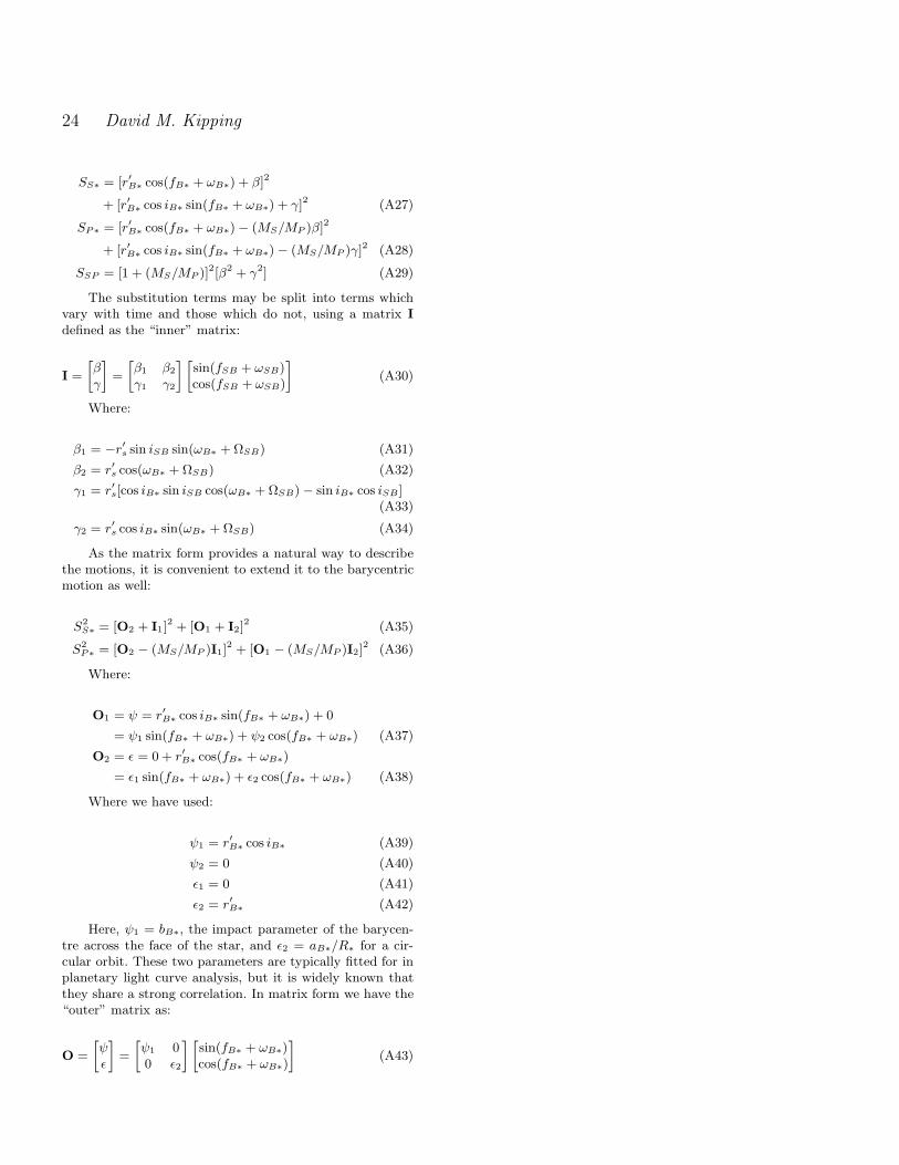
24 David M. Kipping

SS∗ = [r′B∗ cos(fB∗ + ωB∗) + β]2

+ [r′B∗ cos iB∗ sin(fB∗ + ωB∗) + γ]2 (A27)

SP∗ = [r′B∗ cos(fB∗ + ωB∗)− (MS/MP )β]2

+ [r′B∗ cos iB∗ sin(fB∗ + ωB∗)− (MS/MP )γ]2 (A28)

SSP = [1 + (MS/MP )]2[β2 + γ2] (A29)

The substitution terms may be split into terms whichvary with time and those which do not, using a matrix I

defined as the “inner” matrix:

I =

[

βγ

]

=

[

β1 β2γ1 γ2

] [

sin(fSB + ωSB)cos(fSB + ωSB)

]

(A30)

Where:

β1 = −r′s sin iSB sin(ωB∗ +ΩSB) (A31)

β2 = r′s cos(ωB∗ + ΩSB) (A32)

γ1 = r′s[cos iB∗ sin iSB cos(ωB∗ + ΩSB)− sin iB∗ cos iSB](A33)

γ2 = r′s cos iB∗ sin(ωB∗ + ΩSB) (A34)

As the matrix form provides a natural way to describethe motions, it is convenient to extend it to the barycentricmotion as well:

S2S∗ = [O2 + I1]

2 + [O1 + I2]2 (A35)

S2P∗ = [O2 − (MS/MP )I1]

2 + [O1 − (MS/MP )I2]2 (A36)

Where:

O1 = ψ = r′B∗ cos iB∗ sin(fB∗ + ωB∗) + 0

= ψ1 sin(fB∗ + ωB∗) + ψ2 cos(fB∗ + ωB∗) (A37)

O2 = ǫ = 0 + r′B∗ cos(fB∗ + ωB∗)

= ǫ1 sin(fB∗ + ωB∗) + ǫ2 cos(fB∗ + ωB∗) (A38)

Where we have used:

ψ1 = r′B∗ cos iB∗ (A39)

ψ2 = 0 (A40)

ǫ1 = 0 (A41)

ǫ2 = r′B∗ (A42)

Here, ψ1 = bB∗, the impact parameter of the barycen-tre across the face of the star, and ǫ2 = aB∗/R∗ for a cir-cular orbit. These two parameters are typically fitted for inplanetary light curve analysis, but it is widely known thatthey share a strong correlation. In matrix form we have the“outer” matrix as:

O =

[

ψǫ

]

=

[

ψ1 00 ǫ2

] [

sin(fB∗ + ωB∗)cos(fB∗ + ωB∗)

]

(A43)

LUNA:Analgorithmfor generatingdynamic planet-moon · PDF fileLUNA:Atransitalgorithmforexomoons...

Documents

Transcript of LUNA:Analgorithmfor generatingdynamic planet-moon · PDF fileLUNA:Atransitalgorithmforexomoons...