CHAPTER 4

Lorentz Correction Factors

In the last chapter, it was demonstrated that electron diffraction amplitudes extracted fromPED patterns with large precession angle φ can be used with direct methods to generate verygood starting structure maps. The only processing necessary is high-pass filtering of low-indexreflections. Multislice simulations showed that — for a much larger range of experimentalthicknesses than conventional diffraction — PED data has low enough error such that it issufficient for use with direct methods without modification. However, the simulations alsoshowed that this is not the case for large thicknesses (> 50 nm), and a correction of theintensities would be required when the crystal is thick.

Precession electron diffraction is intended for finding initial starting structures from un-known materials, therefore in practice usually very little a priori information about the struc-ture will be known when first investigating a novel material. The thickness is another pieceof information that is almost always missing. Any practical correction factor must thereforebe based upon a simple model that is highly tolerant of error within the input parameters. Inother words, what is sought is a well-conditioned model.

While the structure of a novel material is not known, useful information is known aboutthe characteristics of the PED experiment. First, the microscopist knows the geometry of theincident intensity, as well as where the major errors in the scattered intensities lie. Additionally,it may be possible to tell during the experiment whether the specimen spans a large range ofthicknesses and/or is uniformly very thick using morphological clues (such as edge effects),thickness fringes, or the presence of diffuse scattering and/or Kikuchi lines. Finally, it is knownthat precession decreases dynamical coupling such that systematic paths are suppressed and, atany given time, usually only one beam is strongly excited. The simplest model that describesthis is a model involving only two beams: the incident and a scattered beam.

In this chapter, the correction factors based upon two-beam approximations will be inves-tigated in detail to understand how they work and when it is appropriate to apply them. Theresults will also give some new insight into how PED itself works. Some of the contents will bea more accurate reworking of the analysis previously done by Gjønnes (1997) and Vincent andMidgley (1994). First, an exact geometrical model will be established that can be evaluatednumerically. This will serve as a reference for comparison with the Gjønnes correction factors.It will initially take the form of a simple kinematical correction and then will be expanded toinclude dynamical two-beam effects. The distinction between the kinematical geometry portion

77

78

(Lorentz) and the dynamical portion will be discussed, then they will be compared to their ana-logues within the Gjønnes correction factors. Lastly, a comparison of these models to multislicesimulation will be given, with the goal of finding the limits of where each model is applicableto real data.

The corrections based upon two-beam dynamical theory, while simple, require that thestructure factorsalready be known. The term forward calculation will be used to describe this,meaning that correction requires the structure factors already be known, which — if they arepreviously known — negates the need for calculating the correction factors in the first place.Nevertheless, the investigations of the particular corrections described in this chapter help toelucidate the nature of PED and represent a much simpler model with which to describe thephysics of precession than the calculation-intensive full dynamical multislice. Additionally, thetolerance for input error is investigated.

4.1. Derivation of Correction Factors

The similarities of PED to powder diffraction were recognized early on by Vincent andMidgley (1994), who proposed the first correction factor for PED in the first paper on PED.This was based upon a two-beam dynamical model intended for correcting powder diffractionintensities (Blackman 1939). This correction factor was revised by Gjønnes (1997) to betterdescribe the geometrical effects and a number of variations of this factor have been used inthe literature (Vincent and Midgley 1994; Gjønnes et al. 1998b,a; Midgley et al. 1998; Gemmiet al. 2003). The version of the Gjønnes correction factor intended for parallel illumination(analagous to the convergent form of the Gjønnes factor in equation 1.30) is

(4.1) Iking ∝ Icorr

g =

g

√1−

(g

2R0

)Ag∫ Ag

0J0(x)dx

Iexpg ,

where g is the reflection vector and Ag = 2πtUg

k (as defined in Gjønnes et al. (1998a)). In thedefinition of Ag, t is the specimen thickness in Angstroms, Ug is the structure factor, and k isthe wavevector magnitude of the incident radiation. Equation 4.1 represents two corrections: 1)a pre-factor to correct for geometry (Lorentz portion) and 2) a two-beam dynamical correction(Blackman portion).

There are two problems with equation 4.1. First note that the value of Ag, which must bedefined absolutely, is critical for calculating the correct value of the integrated intensity. Aspointed out in section 1.4.2, the argument of the integrand in equation 4.1 is different from thatused in the Blackman formula (equation 1.24) by a factor of two, altering the periodicity of theBessel function J0. The forms of Ag used in Gjønnes (1997) and Gjønnes et al. (1998b) hadconflicting definitions and, furthermore, the structure factors (Ug) that were used to define Ag

had not been clearly defined. Without knowledge of the pre-factor constants, the correctnessof Ag in these studies is not certain. The second problem is that an assumption has been

79

made that the geometry effects can be separated from the dynamical scattering effects. Theconditions for this approximation to hold were not specified in the derivation of the correctionfactor (Gjønnes 1997).

In this section, the correction will be re-derived using kinematical and two-beam electrondiffraction theory. The re-derivation is more exact than the previous models and will be used toexplore the limits of their approximation. For completeness, the original derivation by Blackman(1939) is included at the end of this section in section 4.1.3. The reader is referred to Gjønnes(1997) for the derivation of the Lorentz portion in equation 4.1.

4.1.1. Kinematical Precession

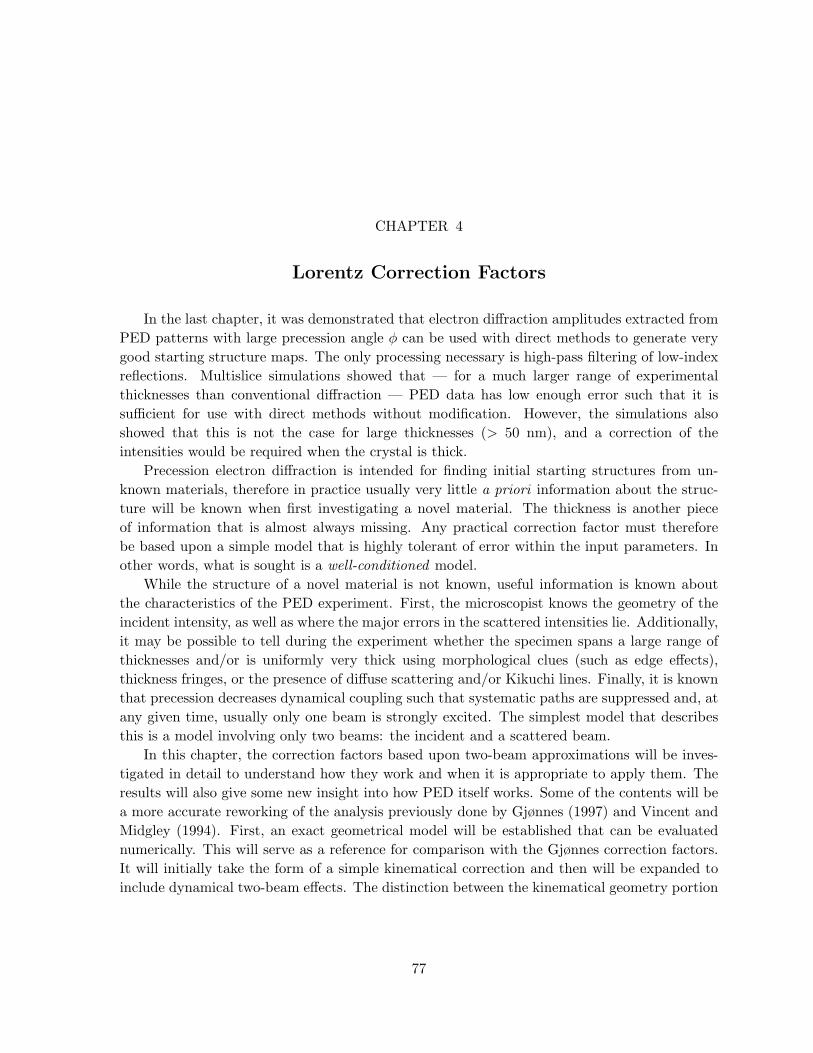
Recall from section 2.1 that the intensity measured in precession represents a finite integrationof the scattered intensity. The relevant geometry, shown previously as figure 2.1, is reproducedhere as figure 4.1. The intensity scattered by the crystal is the true intensity Fg

2 multipliedby some function dependent upon specimen dimensions. Intensity is scattered when this shapefunction — which manifests in reciprocal space as a rod shape (relrod) — is intercepted bythe Ewald sphere. The true intensity can also be recovered by dividing the measured intensityby the value of the shape function at the interception point, described by excitation error sg.Similarly, the true intensity can be recovered from the measured integrated intensity from PEDby dividing by the integrated shape function, in other words

(4.2) |Fg|2 ∝ Icorrg = C(g, t, φ)Iexp

g ,

where Cg is inversely proportional to the precession integral of the shape function of the scat-tered intensity.

In this derivation, we seek to evaluate the integral of the scattered intensity over excitationerror that occurs during the precession:

(4.3) Iprecg =

∫Ig(sg)dsg.

Equation 4.3 is more conveniently treated as an integration over the precession variable θ

representing the circuit traced by the Laue circle, given by

(4.4) Iprecg =

∫ 2π

0I(θ)dθ.

The change of variables can be made starting from the equation of the Ewald sphere:

(4.5) (x− kx)2 + y2 + (z − kz)2 = k2,

80

Figure 4.1. Reciprocal space geometry in (a) x− y plane and (b) x− z plane.The beam precesses about the z-axis maintaining constant φ. In (b), the ZOLZ(bold dashed circle) precesses about the z-axis.

where k = 1/λ, and kx and kz represent the deviation of the Ewald sphere origin in x andz, respectively, due to precession. For a reflection g located at (x, y) = (|g| cos θ, |g| sin θ), theCartesian variables can be converted to functions of θ starting with the substitution

81

(4.6) (g cos θ − kx)2 + (g sin θ)2 + (z − kz)2 = k2.

Simplifying using geometric identities, substituting sg for z, and utilizing |kx|2 + |kz|2 = |k|2,this reduces to

(4.7) g2 − 2kxg cos θ − 2kzsg = 0,

where s2 is very small and has been eliminated from the previous equation. Since kz ≈ k, andkx ≈ kφ in the limit of small φ, this is rearranged to get excitation error as a function of θ:

(4.8) sg(θ) =g2 − 2kφg cos θ

2k.

In kinematical scattering theory, the relrods representing the scattered intensity are de-scribed by the inversion of the top hat function, therefore

(4.9) I(sg) =1ξ2g

sin2(πtsg)sg2

.

The characteristic length ξg (also called the extinction distance) is a function of the experimentalvariables structure factor Fg, unit cell volume Vc, electron wavelength λ, and Bragg angle θB

given by

(4.10) ξg =πVc cos θB

λFg.

The correction factor follows from equations 4.8 and 4.9, giving

(4.11)∫ 2π

0I(θ)dθ =

1ξ2g

∫ 2π

0

sin2{πt(

g2−2kφg cos θ2k

)}(

g2−2kφg cos θ2k

)2 dθ ≡ 1Ckin(g, t, φ)

.

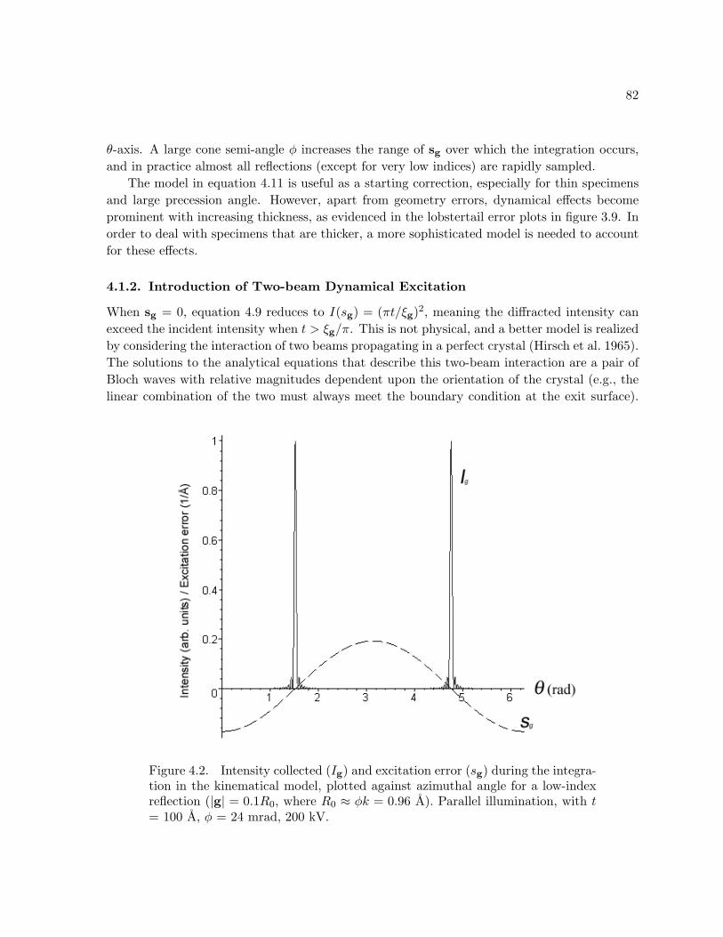
In equation 4.11, the function within the integral over θ yields two peaks, illustrated infigures 4.1(b) and 4.2. A relrod with g < 2R0 enters the zeroth Laue ‘bowl’ once and then exitsonce as θ traverses 2π. The excitation error, describing the deviation from the Bragg scatteringcondition, traces a cosine curve shifted in the z-axis due to the curvature of the Ewald sphereand scaled depending upon distance of the reflection from the origin (equation 4.8). During theprecession, reflections close to the origin are sampled slowly with smaller excitation error, so theshape of the modulus-squared of the sinc function along the θ-axis is widened and more intensityis sampled per unit time from low-g reflections than from high-g reflections. The higher-indexreflections are more rapidly sampled, hence the squared sinc functions are very narrow in the

82

θ-axis. A large cone semi-angle φ increases the range of sg over which the integration occurs,and in practice almost all reflections (except for very low indices) are rapidly sampled.

The model in equation 4.11 is useful as a starting correction, especially for thin specimensand large precession angle. However, apart from geometry errors, dynamical effects becomeprominent with increasing thickness, as evidenced in the lobstertail error plots in figure 3.9. Inorder to deal with specimens that are thicker, a more sophisticated model is needed to accountfor these effects.

4.1.2. Introduction of Two-beam Dynamical Excitation

When sg = 0, equation 4.9 reduces to I(sg) = (πt/ξg)2, meaning the diffracted intensity canexceed the incident intensity when t > ξg/π. This is not physical, and a better model is realizedby considering the interaction of two beams propagating in a perfect crystal (Hirsch et al. 1965).The solutions to the analytical equations that describe this two-beam interaction are a pair ofBloch waves with relative magnitudes dependent upon the orientation of the crystal (e.g., thelinear combination of the two must always meet the boundary condition at the exit surface).

Figure 4.2. Intensity collected (Ig) and excitation error (sg) during the integra-tion in the kinematical model, plotted against azimuthal angle for a low-indexreflection (|g| = 0.1R0, where R0 ≈ φk = 0.96 A). Parallel illumination, with t= 100 A, φ = 24 mrad, 200 kV.

83

The scattered intensity is governed by a new deviation parameter called the effective excitationerror, defined as

(4.12) seffg =

√s2g −

1ξ2g.

The effective excitation error modifies equation 4.9 to account for dynamical exchangebetween the transmitted and diffracted beams, giving

(4.13) I(sg) =1ξ2g

sin2(πtseffg )

(seffg )2

.

When ξg > t, the scattered intensity behaves like a conventional sinc function (with newscaling and periodicity — see the solid curve in figure 4.3). However, when ξg < t, the scatteredintensity at zero excitation error begins to fall, creating a minimum between two nodes centeredabout sg = 0 for some combinations of t and ξg. The most dramatic change occurs when theargument of the sine function in the numerator of equation 4.13 becomes nπ, where n is aninteger (e.g., t

ξg= n), at which point the scattered intensity at sg = 0 falls to zero (dashed

curve in figure 4.3).

Figure 4.3. Scattered intensity (Ig) v. excitation error (sg). Thickness t = 500.For the solid curve ξg = 1500 A and for the dashed curve ξg = 500 A (intensitiesnot to scale). The binodal behavior occurs when t > ξg.

84

The two-beam correction factor for precession thus comprises the integration along sg ofintensity profiles that vary with the extinction distance and specimen thickness (extinctiondistance is in turn inversely proportional to the structure factor). It models the exchange ofintensity between the diffracted and transmitted beams and is valid when only one beam isstrongly excited. Substituting 4.12 in 4.11, the exact two-beam correction factor is obtained:

(4.14)∫ 2π

0I(θ)dθ =

1ξ2g

∫ 2π

0

sin2(πtseffg )

(seffg )2

dθ ≡ 1C2beam(g, t, φ)

.

4.1.3. The Blackman Formula Revisited

In the early paper by Blackman (1939), the intensities of powder rings were elegantly describedby two-beam dynamical theory. Using the same approach as presented in the previous sec-tion, the Blackman formula arises from a simple identity of the integrated scattered intensity.Equation 4.13 can be rewritten in slightly different form:

(4.15) Ig = I0sin2Ag

√(W 2 + 1)

W 2 + 1.

Here, I0 is the incident beam intensity, assumed to be 1 in equation 4.13, Ag = πtξg∝ Fgt, and

W = sgξg. In powder and polycrystal diffraction, each constituent crystal is illuminated offof the zone axis by some angle φ, causing a corresponding excitation error for a given g. Asimple change of variables gives the excitation error as a function of this angle: sg = 2kθφ. Ifthe crystal is rocked with angular speed ω = dφ

dt , the total reflected intensity becomes

Itot =I0ω

∫ +∞

−∞

sin2(Ag

√(W 2 + 1))

W 2 + 1dφ

∝ I02k2θω

Fg

Vc

∫ +∞

−∞

sin2(Ag

√(W 2 + 1))

W 2 + 1dW.(4.16)

The integration of the sinc function in equation 4.16 is equivalent to π times the integralfrom 0 to Ag of the zeroth order Bessel function. This identity gives the basic form of theBlackman formula:

Itot = Idyng =

πI02k2θω

Fg

Vc

∫ Ag

0J0(2x)dx

∝ Ag

∫ Ag

0J0(2x)dx.(4.17)

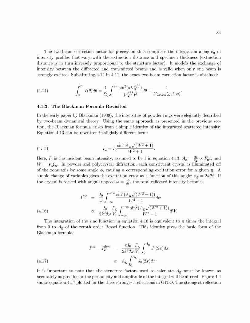
It is important to note that the structure factors used to calculate Ag must be known asaccurately as possible or the periodicity and amplitude of the integral will be altered. Figure 4.4shows equation 4.17 plotted for the three strongest reflections in GITO. The strongest reflection

85

has the greatest average intensity, and the average intensities decrease with decreasing structurefactor. Note that in some thickness ranges such as 350-500 A, the intensity of the strongestreflection drops below that of the next-strongest reflections.

The plots in figure 4.4 represent the Bessel integral for exact thickness values, however inreal specimens there is usually some thickness variation ∆t . The effect of thickness averagingon equation 4.17 in PED has previously been pointed out by Gjønnes et al. (1998b). In thismodel, ∆t will generate a range of oscillation periodicities; superposition of scattered intensityfrom a range of thicknesses generates an effective curve that has reduced oscillation amplitudeand slightly decreased intensity. The behavior at small Ag, however, will remain essentially thesame. In other words, the integral scales linearly with Ag regardless of thickness variation forsmall Ag, but for large Ag the oscillations are damped and converge more rapidly to their finalvalue when ∆t 6= 0. This is advantageous because strong reflections will more likely maintain

Figure 4.4. Equation 4.17 plotted for the three strongest reflections in GITO.The oscillation periodicities are slightly different because the extinction distanceξg varies between reflections. The extinction distances are 580 A, 660 A, and780Afor the 401, 003, and 206 reflections, respectively.

86

kinematical phase relationships between each other when there is some variation in thickness(recall equation 1.27).

4.2. Comparison between models

Five models of precession have now been discussed. To summarize, they are:

• Finite integration limits:(1) Kinematical integral over sg (Lorentz portion);(2) Dynamical (two-beam) integral over seff

g ;• Gjønnes form:

(3) Lorentz portion (approximation of (1));(4) Lorentz and Blackman combined (approximation of (2); the Blackman por-

tion has infinite integration limits);• (5) Multislice (described in chapter 3).

Table 4.1 shows the different forms of the correction and some nomenclature by which torefer to them in the following sections. The fact that the Blackman formula also representsan integration of the two-beam condition is understood. However, for naming convenience,correction (2) will be denoted C2beam while correction (4) will be denoted CBlackman.

The multislice model is exact and effectively describes the physical behavior of PED, asdemonstrated in section 3.2. Multislice will serve as the reference for comparing the approximatemodels listed above. We begin with a general discussion of their relationships, looking at trendsfrom a theoretical standpoint. Later in this section, these relationships will be proven in practiceby comparing the effectiveness of the correction factors at linearizing the simulated datasets.

4.2.1. Expected Trends

The integration limits along sg are an important characteristic within the proposed models.Assuming for the time being that the scattered intensity in precession is always either kine-matical or two-beam in nature (not n-beam where n > 2), the corrections CGj and CBlackman

approximate the more exact corrections Ckin and C2beam only if the precession has integratednearly all of the scattered intensity. The conditions where this is satisfied are investigatedbelow.

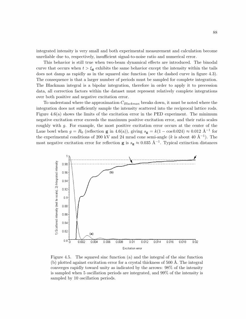
Figure 4.5 shows the behavior of the integral of the squared sinc function as a function ofthe integration limits. Most of the intensity is contained within the first period of the sincfunction, and 98% of the intensity is sampled by integrating 5 periods. Beyond 5 periods, theintegral converges toward unity more slowly, and 99% of the intensity is sampled only afterintegrating 10 oscillation periods. Depending upon the detector sensitivity and the amountof thickness averaging, experimental error is often within 3-5%, hence the integral can beconsidered complete as long as 5-10 periods are sampled and the sampled periods include theregion near sg = 0. The latter constraint arises because the correction factors are inverselyrelated to the integrated intensity; if only a tail of the squared sinc function is sampled, the

87

Tab

le4.

1.C

orre

ctio

nfa

ctor

sfo

rco

rrec

ting

PE

Din

tens

itie

s.N

oteC

Bla

ckm

an

has

corr

ecte

din

tegr

and.

Mon

iker

Typ

eE

q uat

ion

no.

F orm

1Fin

ite

kin

Go e

met

ryon

ly4.

11C

kin

(g,t,φ

)=( 1 ξ

2 g

∫ 2π 0si

n2

πt(

s g)

(sg)2

dθ) −1

2Fin

ite

dyn

F ull

corr

ecti

on4.

14C

2be

am

(g,t,φ

)=( 1 ξ

2 g

∫ 2π 0si

n2(π

tsef

fg

)

(sef

fg

)2dθ) −1

3G

j ønn

esG

eom

etry

only

4.1

CG

j(g,φ

)=

g√ 1−( g

2R

0

)

4G

jønn

es×

Bla

ckm

anFu

llco

rrec

tion

4.1

CB

lack

man(g,t,φ

)=

g√ 1−( g

2R

0

)A

g∫ A g 0

J0(2x)dx

5M

u lti

slic

eE

x act

1.16

non e

(exa

ct)

88

integrated intensity is very small and both experimental measurement and calculation becomeunreliable due to, respectively, insufficient signal-to-noise ratio and numerical error.

This behavior is still true when two-beam dynamical effects are introduced. The binodalcurve that occurs when t > ξg exhibits the same behavior except the intensity within the tailsdoes not damp as rapidly as in the squared sinc function (see the dashed curve in figure 4.3).The consequence is that a larger number of periods must be sampled for complete integration.The Blackman integral is a bipolar integration, therefore in order to apply it to precessiondata, all correction factors within the dataset must represent relatively complete integrationsover both positive and negative excitation error.

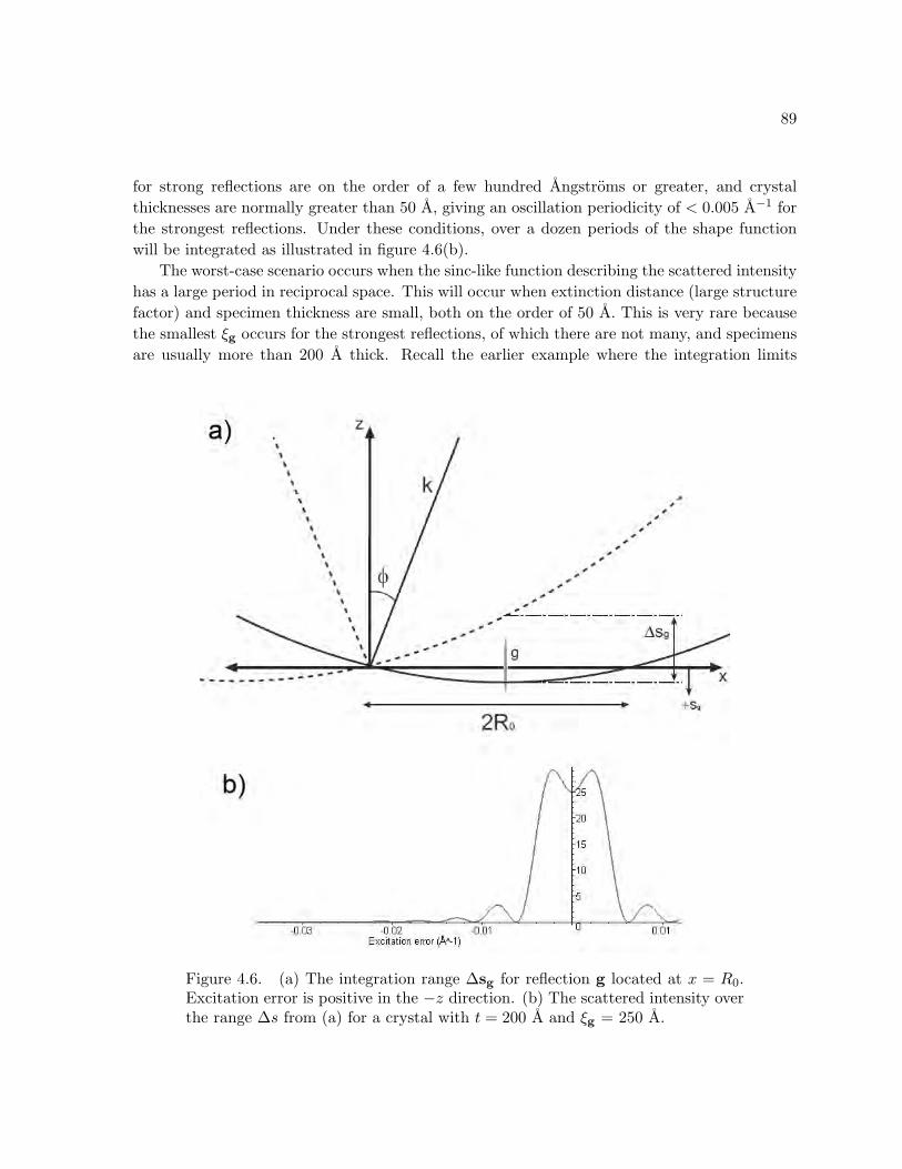
To understand where the approximation CBlackman breaks down, it must be noted where theintegration does not sufficiently sample the intensity scattered into the reciprocal lattice rods.Figure 4.6(a) shows the limits of the excitation error in the PED experiment. The minimumnegative excitation error exceeds the maximum positive excitation error, and their ratio scalesroughly with g. For example, the most positive excitation error occurs at the center of theLaue bowl when g = R0 (reflection g in 4.6(a)), giving sg = k(1 − cos 0.024) ≈ 0.012 A−1 forthe experimental conditions of 200 kV and 24 mrad cone semi-angle (k is about 40 A−1). Themost negative excitation error for reflection g is sg ≈ 0.035 A−1. Typical extinction distances

Figure 4.5. The squared sinc function (a) and the integral of the sinc function(b) plotted against excitation error for a crystal thickness of 500 A. The integralconverges rapidly toward unity as indicated by the arrows: 98% of the intensityis sampled when 5 oscillation periods are integrated, and 99% of the intensity issampled by 10 oscillation periods.

89

for strong reflections are on the order of a few hundred Angstroms or greater, and crystalthicknesses are normally greater than 50 A, giving an oscillation periodicity of < 0.005 A−1 forthe strongest reflections. Under these conditions, over a dozen periods of the shape functionwill be integrated as illustrated in figure 4.6(b).

The worst-case scenario occurs when the sinc-like function describing the scattered intensityhas a large period in reciprocal space. This will occur when extinction distance (large structurefactor) and specimen thickness are small, both on the order of 50 A. This is very rare becausethe smallest ξg occurs for the strongest reflections, of which there are not many, and specimensare usually more than 200 A thick. Recall the earlier example where the integration limits

Figure 4.6. (a) The integration range ∆sg for reflection g located at x = R0.Excitation error is positive in the −z direction. (b) The scattered intensity overthe range ∆s from (a) for a crystal with t = 200 A and ξg = 250 A.

90

were -0.035 A−1 and 0.012 A−1 for a reflection at g = R0. For a material with t = 250 A andξg = 60 A, only about 7 oscillations will be integrated and the Gjønnes corrections will havegreater than 15% error. For GITO, which has a very large unit cell volume, and correspondinglylarge extinction distance of 580 A for its strongest reflection (index 401), the intensity will besufficiently integrated under most experimental conditions.

When g > 2R0, positive excitation error does not occur. Corrections CGj and CBlackman

break down beyond this point and are no longer applicable. However, the correction factorswith finite integration limits (Ckin and C2beam) will still be applicable slightly beyond 2R0

because the negative half of the sinc function is still integrable. Nevertheless, the correctionfactor will soon blow up beyond 2R0 and will be much less practical than simply extendingthe ZOLZ radius by increasing the cone angle φ (figure 4.7). In other words, the precessionangle should be chosen such that the largest g of interest in the diffraction pattern is smallerthan 2R0 by at least 0.25R0. Reflections with sufficient intensity to be measurable are typicallywithin about 1.5 A−1, so φ = 20-25 mrad (at 200kV) is the minimum acceptable angle for PEDstudies where correction factors are applied.

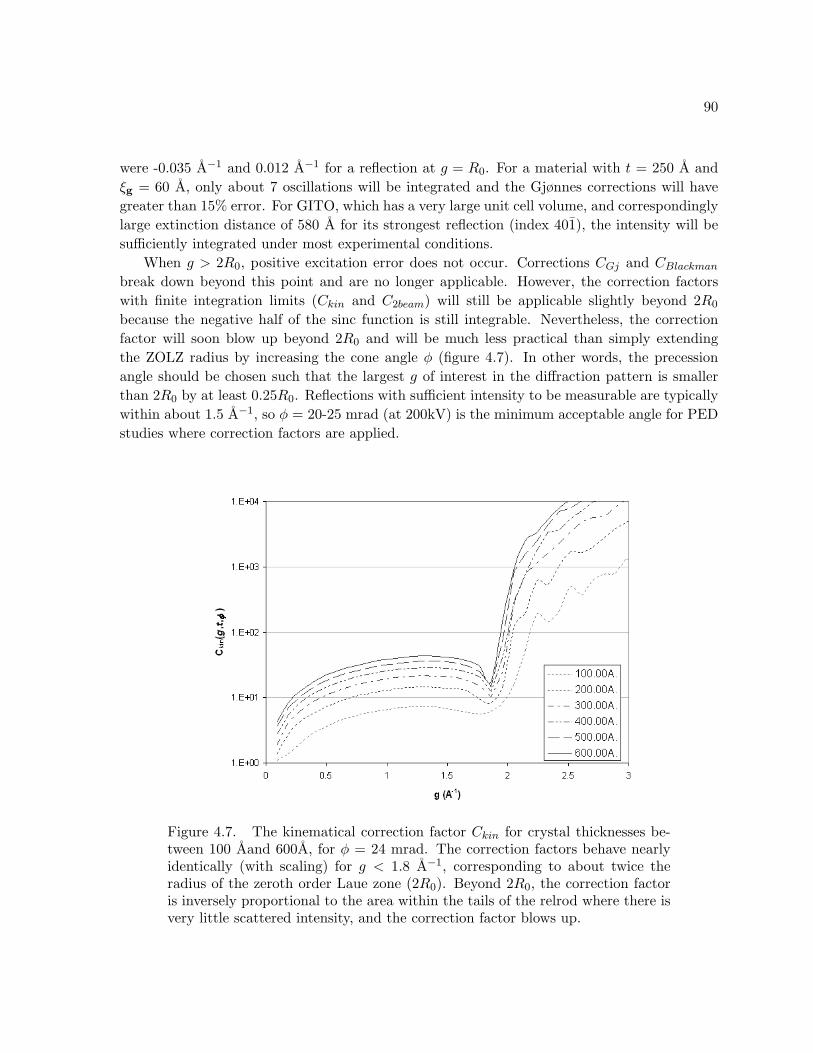
Figure 4.7. The kinematical correction factor Ckin for crystal thicknesses be-tween 100 Aand 600A, for φ = 24 mrad. The correction factors behave nearlyidentically (with scaling) for g < 1.8 A−1, corresponding to about twice theradius of the zeroth order Laue zone (2R0). Beyond 2R0, the correction factoris inversely proportional to the area within the tails of the relrod where there isvery little scattered intensity, and the correction factor blows up.

91

Exploring cone angle selection further, recall that the structurally important reflectionsgenerally fall within the band g = 0.25-1.5 A−1, so it is advantageous to have larger coneangle to increase the positive limit of integration within this band (e.g., deepen the Lauebowl). Furthermore, recall from chapter 3 that going off-zone reduces simultaneous excitation ofmultiple strong reflections, thereby reducing amplitude errors in the PED dataset. Fortuitously,the constraints necessary for good integration coincide with the reduction of dynamical effects:large cone angle improves the correction factors by extending the integration limits along sg,and additionally reduces multiple scattering effects such that two-beam theory is adhered tobetter.

4.2.2. Comparison of Calculated Corrections Factors

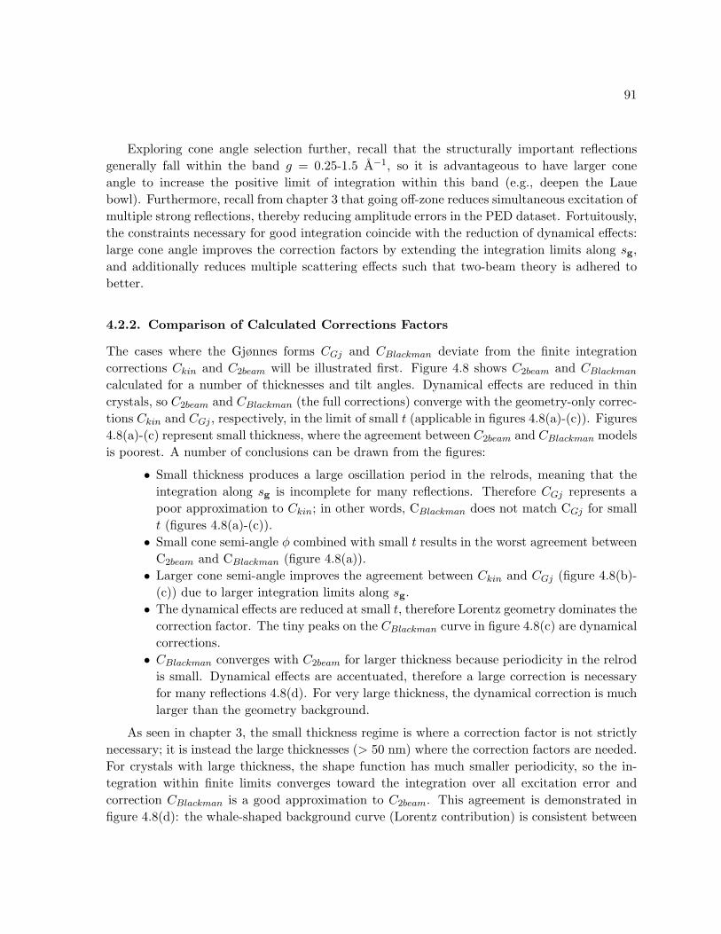
The cases where the Gjønnes forms CGj and CBlackman deviate from the finite integrationcorrections Ckin and C2beam will be illustrated first. Figure 4.8 shows C2beam and CBlackman

calculated for a number of thicknesses and tilt angles. Dynamical effects are reduced in thincrystals, so C2beam and CBlackman (the full corrections) converge with the geometry-only correc-tions Ckin and CGj , respectively, in the limit of small t (applicable in figures 4.8(a)-(c)). Figures4.8(a)-(c) represent small thickness, where the agreement between C2beam and CBlackman modelsis poorest. A number of conclusions can be drawn from the figures:

• Small thickness produces a large oscillation period in the relrods, meaning that theintegration along sg is incomplete for many reflections. Therefore CGj represents apoor approximation to Ckin; in other words, CBlackman does not match CGj for smallt (figures 4.8(a)-(c)).

• Small cone semi-angle φ combined with small t results in the worst agreement betweenC2beam and CBlackman (figure 4.8(a)).

• Larger cone semi-angle improves the agreement between Ckin and CGj (figure 4.8(b)-(c)) due to larger integration limits along sg.

• The dynamical effects are reduced at small t, therefore Lorentz geometry dominates thecorrection factor. The tiny peaks on the CBlackman curve in figure 4.8(c) are dynamicalcorrections.

• CBlackman converges with C2beam for larger thickness because periodicity in the relrodis small. Dynamical effects are accentuated, therefore a large correction is necessaryfor many reflections 4.8(d). For very large thickness, the dynamical correction is muchlarger than the geometry background.

As seen in chapter 3, the small thickness regime is where a correction factor is not strictlynecessary; it is instead the large thicknesses (> 50 nm) where the correction factors are needed.For crystals with large thickness, the shape function has much smaller periodicity, so the in-tegration within finite limits converges toward the integration over all excitation error andcorrection CBlackman is a good approximation to C2beam. This agreement is demonstrated infigure 4.8(d): the whale-shaped background curve (Lorentz contribution) is consistent between

92

Fig

ure

4.8.

Com

pari

son

ofth

efu

llco

rrec

tion

fact

orsC

2be

am

andC

Bla

ckm

an

from

tabl

e4.

1pl

otte

dag

ains

tg.

(a)-

(c)

Dyn

amic

aleff

ects

are

smal

lw

hent

issm

all,

ther

efor

eth

efu

llco

rrec

tion

sco

nver

getoC

kin

and

CG

j,r

espe

ctiv

ely.

The

plot

ssh

owth

atC

Gj

does

not

mat

chth

eC

kin

wel

lat

smal

lthi

ckne

ss.

(c)

For

larg

erti

ltan

gle,

Gjø

nnes

-Bla

ckm

anco

rrec

tion

mat

ches

forg<R

0.

Smal

lpe

aks

begi

nto

appe

aron

top

ofth

ege

omet

ryte

rm(w

hale

-sha

ped

curv

e)as

thic

knes

sin

crea

ses.

(d)

Cor

rect

ionC

Bla

ckm

an

mat

ches

corr

ecti

onC

2be

am

forla

rge

thic

knes

sbe

caus

eth

epe

riod

icity

wit

hin

the

relr

odis

very

smal

l.T

hedy

nam

ical

corr

ecti

ons

(pea

ks)

dom

inat

eth

eco

rrec

tion

fact

orva

lues

.

93

the two corrections at 634 A, and the peaks match to within a few percent. Note that thecorrections are plotted as curves to accentuate the peaking and the correction factors are notreally continuous: each peak represents a correction for a specific reflection.

At large thickness, dynamical effects naturally begin to dominate. This is clearly seen infigure 4.8(d), where many reflections within the structure-defining regime 0.25-0.75 A−1 havelarge corrections above the background curve. The key observation is that the correction factorselectively corrects reflections that have large error due to dynamical scattering. A secondmajor point is that at large thickness, where relrods have small oscillation period, the geometrycan indeed be separated from the thickness-dependent dynamical effects and the geometry canbe approximated in the limit of moderate-to-large thickness by CGj which is independent ofthickness. The net correction is reduced to the product between the Lorentz and Blackmanterms.

Figure 4.9 shows the trends in more detail using plots of C2beam for various thicknesses(increasing horizontally) and cone angles (increasing down each column). The thicknesses arelarge enough that CBlackman is a good approximation and will yield similar results for all plotsexcept the top left (φ = 10 mrad, t = 32 nm). Small cone angles yield incomplete integration ofscattered intensity and the errors become substantial beyond g = 2R0. The integration is fairlycomplete with larger cone angle, evidenced by the decay of dynamical-type corrections (spikes)at higher g within the plots. Large corrections are necessary for the reflections in the structure-defining range of 0.25-1 A−1. For very thick crystals (right-most column), dynamical effectsextend out to very high spatial frequencies in the diffraction pattern, and their correctionsextend to greater g correspondingly.

4.2.3. Application to Multislice Data Sets

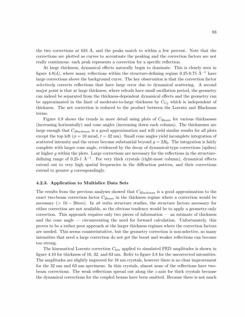
The results from the previous analyses showed that CBlackman is a good approximation to theexact two-beam correction factor C2beam in the thickness regime where a correction would benecessary (> 10 − 20nm). In ab initio structure studies, the structure factors necessary foreither correction are not available, so the obvious tendency would be to apply a geometry-onlycorrection. This approach requires only two pieces of information — an estimate of thicknessand the cone angle — circumventing the need for forward calculation. Unfortunately, thisproves to be a rather poor approach at the larger thickness regimes where the correction factorsare needed. This seems counterintuitive, but the geometry correction is non-selective, so manyintensities that need a large correction do not get the boost and weaker reflections can becometoo strong.

The kinematical Lorentz correction Ckin applied to simulated PED amplitudes is shown infigure 4.10 for thickness of 16, 32, and 63 nm. Refer to figure 3.8 for the uncorrected intensities.The amplitudes are slightly improved for 16 nm crystals, however there is no clear improvementfor the 32 nm and 63 nm specimens. In thin crystals, almost none of the reflections have two-beam corrections. The weak reflections spread out along the z-axis for thick crystals becausethe dynamical corrections for the coupled beams have been omitted. Because there is not much

94

Figure 4.9. Tableau of correction factor plots for the GITO system calculatedfor various cone semi-angles and specimen thickness. The constituent plots rep-resent C2beam v. g. The plots in the 10 mrad row have a cutoff of g = 0.9 A−1

because for small cone semi-angle the correction factor blows up at high spatialfrequencies.

correlation between precession geometry and the beam intensity, the strongly coupled beamswill receive insufficient correction under most circumstances.

This helps to explain why the R-factors were much worse in the AlmFe and Ti2P studiesusing intensities corrected only for geometry (Gjønnes et al. 1998a; Gemmi et al. 2003) versusthe AlmFe study utilizing the full correction (Gjønnes et al. 1998b). The reported R1 valuesfor the structures found using CGj-corrected intensities were 42% and 36%, respectively, versus32% for the structure found using CBlackman. The most uncertain step in the first two studieswas the merging of multiple projections. This is to be expected with the crystal thickness onthe order of 100 nm. The two-beam dynamical effects would be severe, and the reliability ofscaling for common reflection is subject highly doubtful. The preferred solution is to simplyuse thinner crystals (e.g., fine probe near the specimen edge) and remove the reflections nearthe transmitted beam instead of treating the intensities for precession geometry.

95

Figure 4.10. Multislice amplitudes with correction factor Ckin applied.

If structure factors are known, as in the case of partially-solved structures or where somestructure factors have been obtained through other means such as CBED, then the C2beam

correction may be used. Figure 4.11 shows the application of the full corrections, some of whichwere shown in figure 4.9, to correct multislice amplitudes from figure 3.8. The top two rows ofplots show that there is some divergence between C2beam and CBlackman at small precession coneangle. This is less of a problem at large thickness, but in any case the error is not more than10%. At larger cone semi-angles of 24 mrad and 75 mrad, C2beam and CBlackman are virtuallyidentical and only C2beam-corrected plots are shown for those cone semi-angles.

The corrections work very well for thicknesses in the regime of 48-100 nm for the GITOstructure. In this regime, the weak reflections still exhibit some residual offset, however theintensity ordering is very good. The residual offset occurs because there is always a smallamount of multi-beam coupling around the ZOLZ ring and the stronger beams will alwayscontribute some intensity to some of the weaker beams through short systematic paths. Thestrongest beams will be weakened slightly as they couple with the weakest beams surroundingthem, giving rise to an apparent curvature in the amplitude reference plots. This effect is mostpronounced in the 50-75 nm thicknesses.

At very large thickness (> 90 nm), the corrected intensities exhibit a minor inflection. Thisis a residual dynamical feature attributed to n-beam intensity exchange. The inflection is less

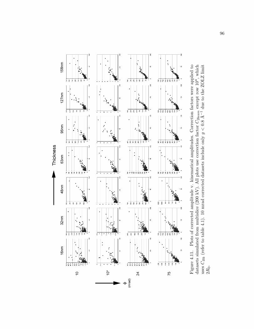
96

Fig

ure

4.11

.P

lots

ofco

rrec

ted

ampl

itud

ev.

kine

mat

ical

ampl

itud

es.

Cor

rect

ion

fact

ors

wer

eap

plie

dto

data

sets

sim

ulat

edfr

omm

ulti

slic

e(2

00kV

).A

llpl

ots

use

corr

ecti

onfa

ctorC

2be

am

exce

ptro

w10

*,w

hich

usesC

Bk

(ref

erto

tabl

e4.

1).

10m

rad

corr

ecte

dda

tase

tsin

clud

eon

lyg<

0.8

A−

1du

eto

the

ZO

LZ

limit

2R0.

97

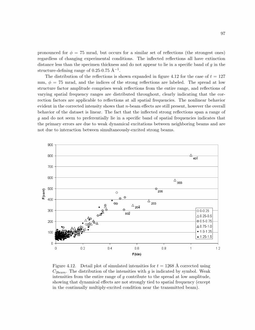
pronounced for φ = 75 mrad, but occurs for a similar set of reflections (the strongest ones)regardless of changing experimental conditions. The inflected reflections all have extinctiondistance less than the specimen thickness and do not appear to lie in a specific band of g in thestructure-defining range of 0.25-0.75 A−1.

The distribution of the reflections is shown expanded in figure 4.12 for the case of t = 127mm, φ = 75 mrad, and the indices of the strong reflections are labeled. The spread at lowstructure factor amplitude comprises weak reflections from the entire range, and reflections ofvarying spatial frequency ranges are distributed throughout, clearly indicating that the cor-rection factors are applicable to reflections at all spatial frequencies. The nonlinear behaviorevident in the corrected intensity shows that n-beam effects are still present, however the overallbehavior of the dataset is linear. The fact that the inflected strong reflections span a range ofg and do not seem to preferentially lie in a specific band of spatial frequencies indicates thatthe primary errors are due to weak dynamical excitations between neighboring beams and arenot due to interaction between simultaneously-excited strong beams.

Figure 4.12. Detail plot of simulated intensities for t = 1268 A corrected usingC2beam. The distribution of the intensities with g is indicated by symbol. Weakintensities from the entire range of g contribute to the spread at low amplitude,showing that dynamical effects are not strongly tied to spatial frequency (exceptin the continually multiply-excited condition near the transmitted beam).

98

An interesting exercise is to investigate the effect of error in the forward calculation. Thisis a crude test for the determining how well-conditioned the correction factor model is. Noisystructure factors were generated using the algorithm

(4.18) Fnoig =

(1 +

e

100× (nrand ∗ 2− 1)

)F kin

g ,

where e is the percent error and nrand is a random number between 0 and 1. The errorintroduced is bipolar and independent of the structure factor, so it is not intended to modeldynamical effects. The R-factors for the structure factors with noise added are given in table 4.2.Each dataset had a different noise profile to control for any serendipitous correction behavior.

The datasets corrected with a C2beam that has been calculated using the noisy structurefactors were then plotted against the true structure factor. Figure 4.13 shows the correctedsimulated datasets with largest noise profiles in the correction factors. R1 values have beencalculated for each set and are given in table 4.3. The R-factors of the corrected data shown inthat table are much lower than the error contained within the inputted data. The improvementis, however, dependent upon the experimental conditions, which means that the geometry termplays a substantial role here. It is important to note that while the approach yields low R-factors, the plots in figure 4.13 indicate that the correction factors do not strongly preserveintensity relationships. This is to be expected, since there is no way that equation 4.14 canpredict the correct structure factor. However, the moderately well-conditioned character ofthis algorithm does make way for a potential iterative correction factor scheme, wherein apoor starting set of structure factors might be refined into more accurate structure factors byapplying a priori constraints and then refining based upon a statistical two-beam dynamicalmodel.

We conclude this section with the mention that the mechanism behind some of the residualdynamical behaviors are not manifestly obvious. For example, the R-factor is lower for largerthickness (also observed qualitatively in figure 4.11). This might be explained by the fact thatthe integral over excitation error converges to a constant in the limit of large t. Under thiscondition, the correction factor behavior is dominated by the prefactor 1/ξg. In other words,equation 4.1 (which holds within the very large thickness regime) becomes

Table 4.2. R1 for the structure factors with noise added using equation 4.18.

Thickness 10% error 20%error 40%error— 24 mrad —

400 9.734 20.122 41.498800 9.800 21.315 39.140

— 75 mrad —400 10.492 20.103 40.601800 10.077 19.266 40.528

99

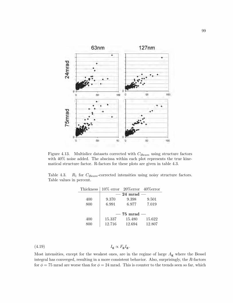
Figure 4.13. Multislice datasets corrected with C2beam using structure factorswith 40% noise added. The abscissa within each plot represents the true kine-matical structure factor. R-factors for these plots are given in table 4.3.

Table 4.3. R1 for C2beam-corrected intensities using noisy structure factors.Table values in percent.

Thickness 10% error 20%error 40%error— 24 mrad —

400 9.370 9.398 9.501800 6.991 6.977 7.019

— 75 mrad —400 15.337 15.480 15.622800 12.716 12.694 12.807

(4.19) Ig ∝ FgIg.

Most intensities, except for the weakest ones, are in the regime of large Ag where the Besselintegral has converged, resulting in a more consistent behavior. Also, surprisingly, the R-factorsfor φ = 75 mrad are worse than for φ = 24 mrad. This is counter to the trends seen so far, which

100

almost universally show that large precession cone angle is favorable. The exact mechanismbehind this is not clear and requires further analysis in a future study.

4.3. Discussion: Approach for Solving Novel Structures

For precession to become a reliable and widespread technique for generating good startingstructure models from electron diffraction data, it must be fast and consistent. Chapter 3showed that it is natively psuedo-kinematical for small-to-moderate thickness regimes, withprimary errors in the range of g < 0.25 A−1. PED offers a new working range of up to40-50 nm crystal dimension, representing a very favorable regime for dealing with real-worldbulk structures. The next step, covered in detail within this chapter, has been to extend thecapabilities to even greater thickness by means of correction factors.

It has been shown here that if structure factors are known, the correction generated by atwo-beam dynamical model is quite successful up to extraordinary thickness (beyond 160 nm).This result proves that PED adheres very closely to two-beam dynamical scattering, especiallyat large thickness and large precession angle. It also shows that the data are affected by n-beameffects, as seen in the structure factor plots where there remain some residual nonlinearities thatdepend upon thickness. The effects, however vary systematically with increasing experimentalthickness and angle, and are slowly varying with changing experimental conditions.

The two-beam dynamical model, while fairly accurate, is unfortunately not immediatelypractical for generating an a priori correction factor for general use. This is because successfulcorrection for large thickness requires a forward calculation: the structure factors must beknown before the crystal structrure can be solved. Nevertheless, the analyses do give somenew tools for enhancing ab initio structure solution using PED and open the way toward lesscomplex iterative structure solution methods than multislice, which requires both structurefactors and phases.

The structure solution in chapter 3 on GITO already made use of a crude form of thecorrection factors that were investigated in this chapter. In section 3.1 a simple modification wasmade to the experimental precession data from GITO (figure 3.4(a)) that appeared to linearizethe measured amplitudes to a kinematical approximation. This simple approach involved usingthe square of the amplitudes — the intensities — instead of the amplitudes to solve with directmethods. The structure maps that were generated from this procedure had identical atompositions to the solution found using high-pass filtered amplitudes, however it more clearlydisplayed some of the atom positions (e.g., clearer peaks) that were very close to the noisefloor in the amplitude solution. This is an interesting behavior for which an explanation is notmanifestly obvious.

The underlying principle can be found by examining the limits of the Blackman formula1.24. By rearranging the Blackman equation, the measured intensity Idyn

g from a crystal ofgreater than moderate thickness (t > 25 nm) becomes

101

(4.20) Idyng ∝ F kin

g

∫ Ag

0J0(2x)dx.

In the limit of large Ag, the integral converges to a constant of 0.5. Therefore, when thethickness is very large or if g is a strong reflection,

(4.21) Idyng ∝ F kin

g .

In effect, even though not all reflections necessarily obeyed equation 4.20, the importantreflections (the strong ones) did and became more linearized toward pseudo-kinematical values.The fact that weaker reflections might not obey equation 4.20 offers a mechanism as to whythe background in figure 3.6 contains noisy oscillations.

In a priori investigations of novel structures, a clear path for how to treat the data has nowbeen elucidated. There is overwhelming evidence that large cone semi-angle φ is beneficial to thequality of the data. Additionally, thin specimens are advantageous because they decrease error,and the thinnest ones (< 15 nm) are easy to treat via a kinematical correction for geometry.The geometry corrections Ckin and Cgj , counterintuitively, are not favorable. The low spatialfrequency reflections contained in the range g < 0.25 A−1, which are usually weak, exhibitthe largest dynamical error because they are near the transmitted beam and are almost alwaysundergoing simultaneous excitation with other beams during the precession experiment. Unlessimportant reflections lie within that range for the structure under investigation, they should behigh-pass filtered regardless of whether correction factors are used.

The requirement for forward calculation is an unfavorable one because precession is still notable to solve novel structures from data that is taken from very thick specimens. The effects areslowly varying with thickness if a large hollow-cone angle is used, and complementary methodscan indicate the approximate thickness regime. Therefore, the conditions giving rise to largedynamical errors in the data can usually be avoided. The major breakthrough from this chapteris that there is strong evidence showing that the structural electron crystallography problem hasbeen reduced from a many-beam problem to a largely two-beam. This is a major simplificationand future methods, keeping in mind that |Fg| is all that is required for the forward calculation,will need to take advantage of this new understanding.

The methods presented in chapter 3 should give favorable starting structure solutions forstructures that project well, e.g., they exhibit the property that intensities that have been lin-earized to a pseudo-kinematical approximation. The use of intensities rather than amplitudesis advantageous in the moderate-to-large thickness range (t = 25-75 nm) if used with largecone angle. This method must, however, be used with caution since dynamical behaviors inuncorrected intensities may be substantial at the top of the thickness range for some materials.A classic example is where two neighboring reflections are both strong: a clear path for strongdynamical exchange exists in such a case. Reflections near the transmitted beam predictablycontain the largest dynamical errors, and in a priori structure studies it is recommended that

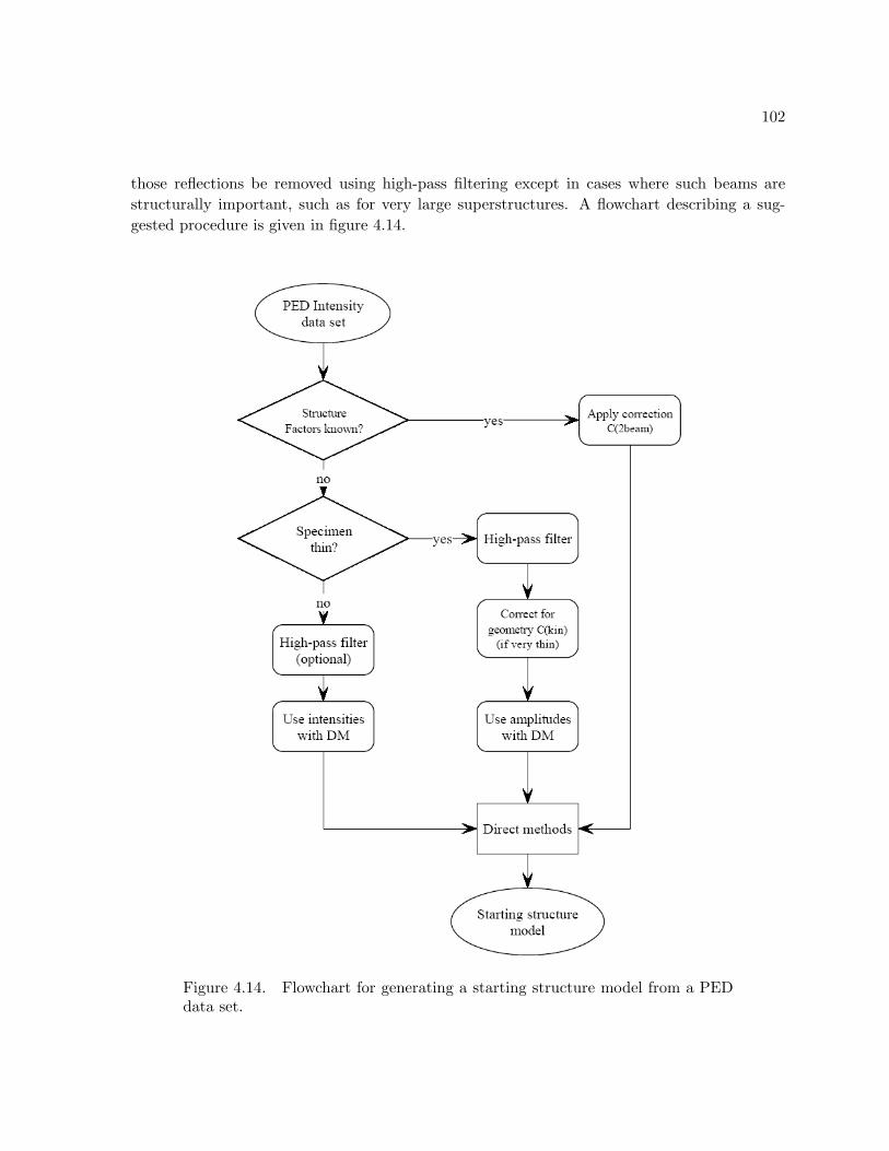
102

those reflections be removed using high-pass filtering except in cases where such beams arestructurally important, such as for very large superstructures. A flowchart describing a sug-gested procedure is given in figure 4.14.

Figure 4.14. Flowchart for generating a starting structure model from a PEDdata set.