1

Paper SAS2023-2018

Looking Beyond the Model with SAS® Simulation Studio: Data Input, Collection, and Analysis

Ed Hughes, SAS Institute Inc.

ABSTRACT

Discrete-event simulation as a methodology is often inextricably intertwined with many other forms of analytics. Source data often must be repaired or processed before being used (indirectly or directly) to characterize variation in a simulation model. Collection of simulated data needs to coordinate with and support the evaluation of performance metrics in the model. Or it might be necessary to integrate other analytics into a simulation model to capture specific complexities in the real-world system that you are modeling.

SAS® Simulation Studio is a component of SAS/OR® software that provides an interactive, graphical environment for building, running, and analyzing discrete-event simulation models. In a broader sense, it is also an integral part of the SAS® analytic platform. This paper illustrates how SAS Simulation Studio enables you to tackle each of these discrete-event simulation challenges. You have full control over the use of input data and the creation of simulated data. Strong experimental design capabilities mean you can simulate for all needed scenarios. In addition, you can embed any SAS analytic program—optimization, data mining, or otherwise—directly into the execution of your simulation model.

INTRODUCTION

Much has been said and written about the intuitive interface and strong modeling capabilities of SAS Simulation Studio. Several recent SAS® Global Forum papers (including Bélanger, Couture, and Neusy 2011; Hevener, Flinchum, and Lada 2013; DeRienzo et al. 2014; and Hughes et al. 2016) have explored the advantages and the practical benefits of modeling with SAS Simulation Studio. However, strength in modeling is just one aspect of SAS Simulation Studio that sets it apart from other discrete-event simulation software.

This paper focuses on how simulation models need to work effectively within their surroundings, because on a practical basis, simulation modeling is never done in isolation. It’s essential that your simulation modeling work effectively coordinates with some equally significant elements of the data and analytic environments in which simulation models are created and used. These include descriptive analytics, predictive analytics, and experimental design.

The paper begins by briefly reviewing key features and capabilities of SAS Simulation Studio. The sections that follow show how SAS Simulation Studio helps you supply input data to a simulation model, fit probability distributions to input data, and produce simulated status and performance data for the system that you are simulating. These sections also describe SAS Simulation Studio’s capabilities in experimental design, which help ensure that you are running your simulation model for a useful set of scenarios. Finally, the paper discusses how SAS Simulation Studio enables you to integrate other forms of analytics directly into your simulation model. The purpose of this integration could be to provide or evaluate input data before the simulation model runs, to analyze output data produced by the simulation model, or to take an active role in the internal decision-making of the simulation model as it runs.

Hands-on experience with discrete-event simulation in general and SAS Simulation Studio specifically is helpful but not necessary for readers of this paper. A general familiarity is sufficient. For more detailed information about SAS Simulation Studio, see the “References” section.

2

SAS SIMULATION STUDIO: KEY FEATURES

SAS Simulation Studio is a Java-based application in SAS/OR that provides an interactive graphical environment for building, running, and analyzing discrete-event simulation models. It was added to SAS/OR in July 2009, and its capabilities have expanded and improved at a steady pace since then. The graphical user interface requires no programming and provides all the tools needed to build, execute, and analyze discrete-event simulation models. An accompanying programmatic interface enables you to run simulation models in batch mode. SAS Simulation Studio is supported on Windows and Linux clients. Windows support began with the first release, and Linux support was added in September 2017 (SAS Simulation Studio 14.3).

GRAPHICAL USER INTERFACE ELEMENTS

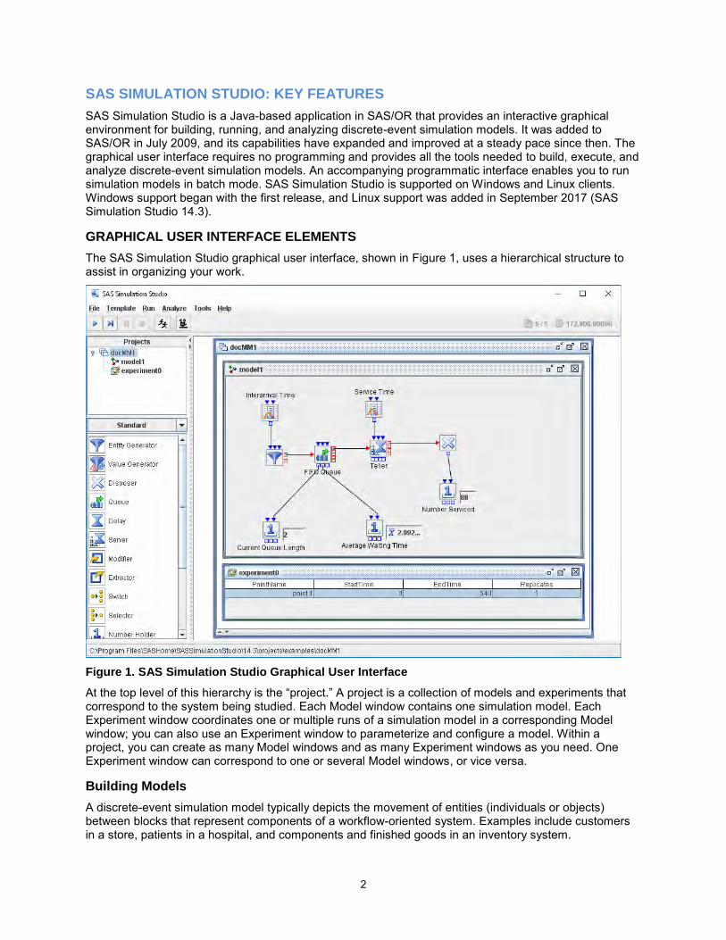
The SAS Simulation Studio graphical user interface, shown in Figure 1, uses a hierarchical structure to assist in organizing your work.

Figure 1. SAS Simulation Studio Graphical User Interface

At the top level of this hierarchy is the “project.” A project is a collection of models and experiments that correspond to the system being studied. Each Model window contains one simulation model. Each Experiment window coordinates one or multiple runs of a simulation model in a corresponding Model window; you can also use an Experiment window to parameterize and configure a model. Within a project, you can create as many Model windows and as many Experiment windows as you need. One Experiment window can correspond to one or several Model windows, or vice versa.

Building Models

A discrete-event simulation model typically depicts the movement of entities (individuals or objects) between blocks that represent components of a workflow-oriented system. Examples include customers in a store, patients in a hospital, and components and finished goods in an inventory system.

3

To build a simulation model in SAS Simulation Studio, you drag blocks from one of five block templates at the left edge of the interface (the Standard template is shown) and drop them in a Model window. You connect the blocks in a model by creating links (again, by dragging and dropping) between ports on the blocks. As shown in Figure 1, links between blue ports on the top and bottom edges of blocks carry data and information; links between red ports on the left and right sides of blocks carry entities. Examples of information flows include inputs such as the service time for a Server block or the interarrival time (time between successive entity arrivals) for an Entity Generator block. Output performance metrics include the current length and the wait time for a Queue block.

Compound blocks and submodels are hierarchical structures that you can add to models. You can group individual blocks into compound blocks to, for example, denote major functional areas or conceal detail (by collapsing compound blocks). You can create multiple independent copies of a compound block and edit them individually. You can also convert a compound block into a submodel, so that any change to its definition is automatically reflected in every copy you have created.

Running Models

You can run a model by using the control menus and buttons at the upper left corner of the SAS Simulation Studio interface (Figure 1). To run a model, first select an Experiment window that has at least one design point in it. For each new project, SAS Simulation Studio creates one Model window and one Experiment window. The Experiment window includes columns that denote the start time, the end time, and the planned number of replicates.

In an Experiment window, you must include the start time, end time, and number of replications to run for a model. If you have created factors to define scenarios for your model and responses to measure its performance, you can include them in a corresponding Experiment window to investigate the effects of varying factor values on responses. This topic is discussed further in the “Experimental Design” section of the paper.

For more information, see Chapter 4, “Simulation Models,” in SAS Simulation Studio 14.3: User’s Guide (SAS Institute Inc. 2017b).

Modeling Resources

Resources (with limited or unlimited capacity) are special objects that provide services of some sort to entities (SAS Institute Inc. 2017b). To increase the realism and depth of detail in models and to maintain model clarity, SAS Simulation Studio enables you to create two types of resources. Stationary resources are blocks (for example, a Queue block or a Server block) that entities visit and occupy temporarily during the run of a simulation model. Mobile resources are a special class of entity—resource entities—that can move between blocks in a simulation model and can be treated in largely the same way as any other entity. An entity seizes and holds a resource entity to indicate that it is occupying the corresponding resource.

Resource entities provide you with many modeling advantages. Although an entity can occupy only one stationary resource block, it can seize and hold an unlimited number of resource entities, and it can continue to do so as it travels through a model. Resource entities can be seized or released at any point in a model. The availability and operational status of a resource entity can change during the run of a model, according to a schedule or randomly. In short, adding resource entities to a model significantly increases your ability to accurately and transparently reflect the use and impact of resources in the system you are modeling.

For more information, see Chapter 10, “Resources,” in SAS Simulation Studio 14.3: User’s Guide (SAS Institute Inc. 2017b).

WORKING WITH DATA

The chief purpose of discrete-event simulation modeling (aside from providing valuable insights, as modeling invariably does) is to produce data on the performance of the system that you are simulating. To ensure that your simulation model realistically depicts the system you want to model, it must include descriptive information that is relevant to the system. Often this takes the form of direct or indirect input

4

data. You might also use predictive data as input in order to, for example, characterize demand in a future period that you want to simulate.

Thus, both input data and output data are vitally important in simulation modeling. SAS Simulation Studio provides you with many ways to supply input data to and write output data from simulation models, and enables you to control when, where, and how input data is used and output data is created.

USING INPUT DATA

Input data plays a critical role in simulation modeling. Input data that describes the structure, internal logic, capacities, or other important characteristics of the system to be simulated is the primary means of ensuring that these elements are accurately depicted in a simulation model. Sometimes this data is drawn from direct observation of a system or an analogue. At other times, the input data might be extrapolated from observed data or based on expert conjecture; this is more likely to occur when a hypothetical system is simulated.

Data Input Methods

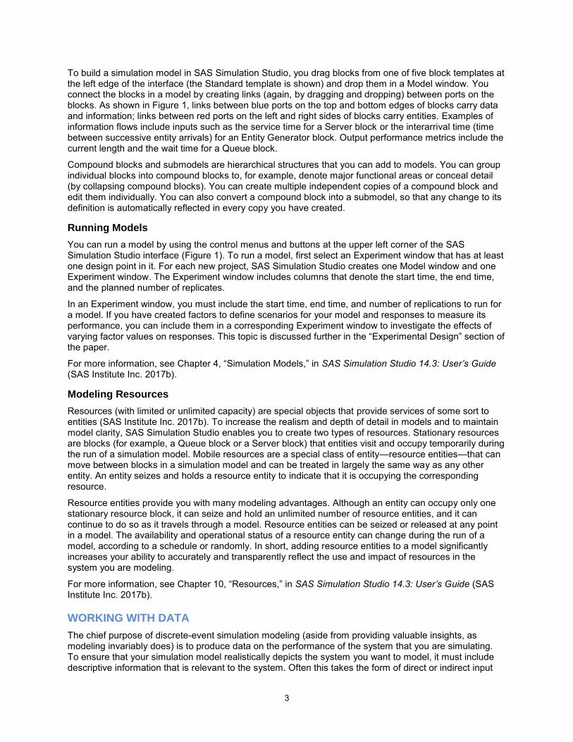
Regardless of the source, SAS Simulation Studio provides you with multiple ways in which to supply input data to a simulation model. The Numeric Source block and the Text Source block read the variable that you designate (numeric or textual, respectively) from a SAS data set or JMP® table. Each time an entity arrives at the block, it advances to the next observation in the data source to read the value of the designated variable. The Observation Source block expands on this mode of operation and reads an entire observation (or row) from the data source. The Observation Source block can be especially useful if you use input data to assign attributes to entities, as shown in Figure 2.

Figure 2. Two Methods of Assigning Attributes to Entities

5

The Observation Source block enables you to assign numerous attributes in one step by connecting a Modifier block to a single Observation Source block instead of multiple Numeric Source blocks and Text Source blocks. In both models in Figure 2, a Modifier block assigns five attributes to each entity; in Model0, three Numeric Source blocks and two Text Source blocks each read one variable from the same input SAS data set and pass the variable’s value to the Modifier block as an independent value.

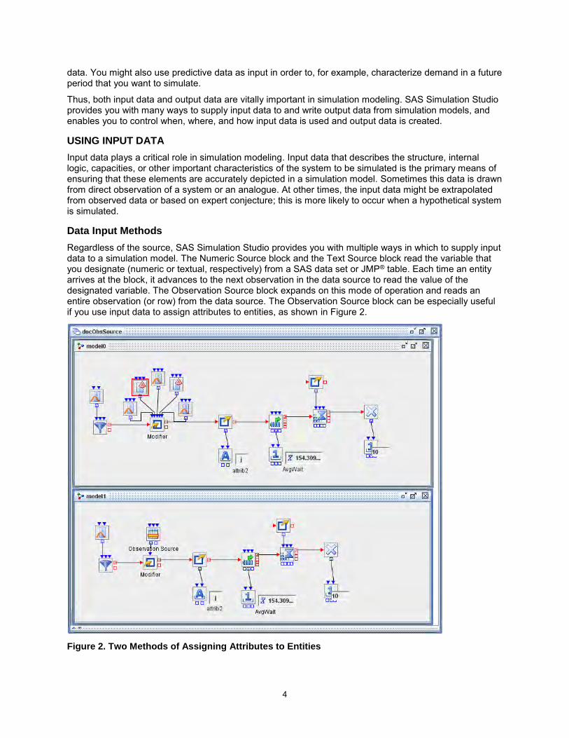
But in Model1, a single Observation Source block reads an entire observation (which contains all five variables) from the same SAS data set and passes the observation to the Modifier block. When a Modifier block accepts an observation as input, you can specify whether to use all or part of the observation to assign attributes, as shown in Figure 3. In this case the Modifier block accepts the entire observation and assigns all five attributes accordingly.

Figure 3. Modifier Block Dialog Box

Another block enables you to move beyond reading a single variable value or a single observation from an input data source. The Dataset Holder block accepts an entire SAS data set or JMP table as input and makes it available for repeated query throughout the run of your simulation model. You can query a selected row or cell (defined by a unique combination of row and column) from the data source, and you can repeat any query as many times as needed.

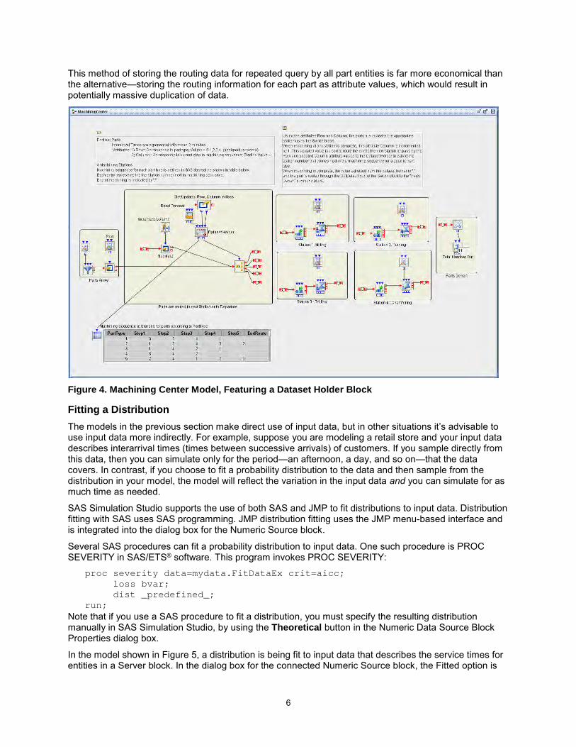
Figure 4 shows a model of a machining center that processes five types of parts at four different stations. Parts of each type visit the stations in a distinct sequence. For example, type 1 parts visit stations 3, 2, 4, and 1, but type 2 parts visit stations 1, 2, 4, 3, and 2. A SAS data set specifies these type-specific sequences. An Observation Source block (labeled “Read Dataset”) reads in the entire data set and passes it to a Dataset Holder block. Each observation of the data set contains the machining sequence for one type of part. The entire routing SAS data set is displayed in the Table block at the lower left corner of the model.

In this model, an entity that represents a part repeatedly queries the row of the Dataset Holder block that corresponds to its type to determine the next station to visit. In each query, the entity reads a single cell from the stored SAS data set; the InRow value that it sends to the Dataset Holder block remains the same, but the InColumn value increases by 1 with each new query. Collectively, the InRow and InColumn values direct the Dataset Holder block to retrieve the value in the data cell that specifies the next station to be visited by the part.

6

This method of storing the routing data for repeated query by all part entities is far more economical than the alternative—storing the routing information for each part as attribute values, which would result in potentially massive duplication of data.

Figure 4. Machining Center Model, Featuring a Dataset Holder Block

Fitting a Distribution

The models in the previous section make direct use of input data, but in other situations it’s advisable to use input data more indirectly. For example, suppose you are modeling a retail store and your input data describes interarrival times (times between successive arrivals) of customers. If you sample directly from this data, then you can simulate only for the period—an afternoon, a day, and so on—that the data covers. In contrast, if you choose to fit a probability distribution to the data and then sample from the distribution in your model, the model will reflect the variation in the input data and you can simulate for as much time as needed.

SAS Simulation Studio supports the use of both SAS and JMP to fit distributions to input data. Distribution fitting with SAS uses SAS programming. JMP distribution fitting uses the JMP menu-based interface and is integrated into the dialog box for the Numeric Source block.

Several SAS procedures can fit a probability distribution to input data. One such procedure is PROC SEVERITY in SAS/ETS® software. This program invokes PROC SEVERITY: proc severity data=mydata.FitDataEx crit=aicc;

loss bvar;

dist _predefined_;

run;

Note that if you use a SAS procedure to fit a distribution, you must specify the resulting distribution manually in SAS Simulation Studio, by using the Theoretical button in the Numeric Data Source Block Properties dialog box.

In the model shown in Figure 5, a distribution is being fit to input data that describes the service times for entities in a Server block. In the dialog box for the connected Numeric Source block, the Fitted option is

7

selected. The File Path field indicates the path to the input data (in this case, a plain text file), and the Column Name field specifies that a distribution should be fitted to the variable named bvar.

Figure 5. Simulation Model and Numeric Source Block Properties Dialog Box

Clicking the Fit Distribution (JMP) button sends this information to JMP and uses the JMP Fit All option to fit distributions to the selected variable. JMP displays the Distribution for Simulation Studio window as shown in Figure 6. (The top and bottom halves of the window are split in this figure.)

Figure 6. JMP Distribution for Simulation Studio Window

8

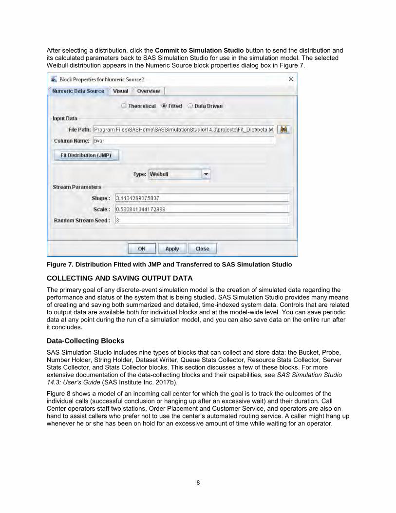
After selecting a distribution, click the Commit to Simulation Studio button to send the distribution and its calculated parameters back to SAS Simulation Studio for use in the simulation model. The selected Weibull distribution appears in the Numeric Source block properties dialog box in Figure 7.

Figure 7. Distribution Fitted with JMP and Transferred to SAS Simulation Studio

COLLECTING AND SAVING OUTPUT DATA

The primary goal of any discrete-event simulation model is the creation of simulated data regarding the performance and status of the system that is being studied. SAS Simulation Studio provides many means of creating and saving both summarized and detailed, time-indexed system data. Controls that are related to output data are available both for individual blocks and at the model-wide level. You can save periodic data at any point during the run of a simulation model, and you can also save data on the entire run after it concludes.

Data-Collecting Blocks

SAS Simulation Studio includes nine types of blocks that can collect and store data: the Bucket, Probe, Number Holder, String Holder, Dataset Writer, Queue Stats Collector, Resource Stats Collector, Server Stats Collector, and Stats Collector blocks. This section discusses a few of these blocks. For more extensive documentation of the data-collecting blocks and their capabilities, see SAS Simulation Studio 14.3: User’s Guide (SAS Institute Inc. 2017b).

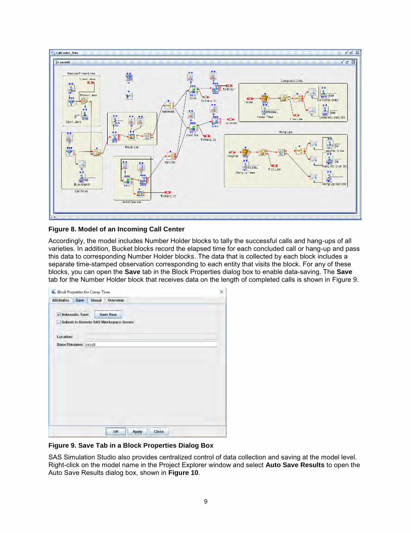
Figure 8 shows a model of an incoming call center for which the goal is to track the outcomes of the individual calls (successful conclusion or hanging up after an excessive wait) and their duration. Call Center operators staff two stations, Order Placement and Customer Service, and operators are also on hand to assist callers who prefer not to use the center’s automated routing service. A caller might hang up whenever he or she has been on hold for an excessive amount of time while waiting for an operator.

9

Figure 8. Model of an Incoming Call Center

Accordingly, the model includes Number Holder blocks to tally the successful calls and hang-ups of all varieties. In addition, Bucket blocks record the elapsed time for each concluded call or hang-up and pass this data to corresponding Number Holder blocks. The data that is collected by each block includes a separate time-stamped observation corresponding to each entity that visits the block. For any of these blocks, you can open the Save tab in the Block Properties dialog box to enable data-saving. The Save tab for the Number Holder block that receives data on the length of completed calls is shown in Figure 9.

Figure 9. Save Tab in a Block Properties Dialog Box

SAS Simulation Studio also provides centralized control of data collection and saving at the model level. Right-click on the model name in the Project Explorer window and select Auto Save Results to open the Auto Save Results dialog box, shown in Figure 10.

10

Figure 10. Auto Save Results Dialog Box

This dialog box provides a hierarchical listing of every data-collecting block in the model. You can enable data collection at a block simply by checking the box next to the block name.

In some cases, you are interested in collecting periodic data that corresponds to system behavior in one or more specific periods during the run of your simulation model. SAS Simulation Studio fully supports the collection of periodic data by providing Boolean input ports on several of the data-collecting blocks that you can use, for example, to signal a block to save or clear its collected data. By controlling how and when blocks save and clear their data, you can create periodic output data.

The project shown in Figure 11 illustrates this technique. In this model, assume that simulated time is measured in minutes. Entities arrive in batches of four, at intervals of one minute. They are assigned attributes (using an Observation Source block), wait in a Queue block, and receive service in a Server block. Before each entity exits the system, it passes through a Bucket block, whose function is to record the entity’s age and other attributes.

As indicated in the Experiment window, this simulation runs for 100 minutes. The factor Num_CheckPts=10 indicates that you want to collect 10 sets of periodic data, and the factor Period_Length=5 specifies that each such set will cover 5 minutes of simulated time. Thus, periodic data is being collected on the first half of the simulation run.

An auxiliary flow in the compound block “Periodic Data Signal” controls periodic data collection. At 5-minute intervals, an auxiliary entity is created and (via a Gate block) causes a Boolean “True” value to be sent to the InSaveNow input port of a Dataset Writer block that receives data from the Bucket block. This signal causes all the data that is currently held by the Bucket block to be saved. A Formula block that is connected to the InPolicy input port of the Dataset Writer block supplies the name “resultN” for the SAS data set that is saved at simulation time N.

11

Figure 11. A Project That Collects and Saves Periodic Data

Next, the Gate block sends another Boolean “True” value to the InClearData input port of the Bucket block, clearing its collected data. Now the Bucket block collects data until the next 5-minute interval elapses, and the process repeats. Ten SAS data sets are created, one for each 5-minute period. Figure 12 shows the data set result35.sas7bdat, which corresponds to the simulated period from just after 30 minutes until precisely 35 minutes—or in mathematical notation, the interval (30,35]. Note that the sum of Age and BirthTime for each entity is the simulated time at which the entity exits the model. For each of the four entities that are described, this sum is in the interval (30,35].

Figure 12. Sample Periodic Data

Model-Wide Output Data Collection Controls

In some cases, you might need to coordinate the control of data collection by several blocks in a model, possibly encompassing all data-collecting blocks in a model. Two additional SAS Simulation Studio blocks are designed to provide you with broad control over how other blocks collect output data. This kind

12

of model-wide control is especially useful when you need to specify when several or all data-collecting blocks in a model should start or stop data collection.

The Data Trimmer block enables you to signal any data-collecting block to clear (reset) all data that it has collected—the equivalent of sending a Boolean “True” value to the block’s InClearData input port. The Data Trimmer block properties dialog box provides a hierarchical check-box listing of every data-collecting block in a model; selected blocks are targeted for data clearing. Whenever a Data Trimmer block receives a Boolean “True” value via its InTrimNow input port, it signals all selected blocks to clear their data.

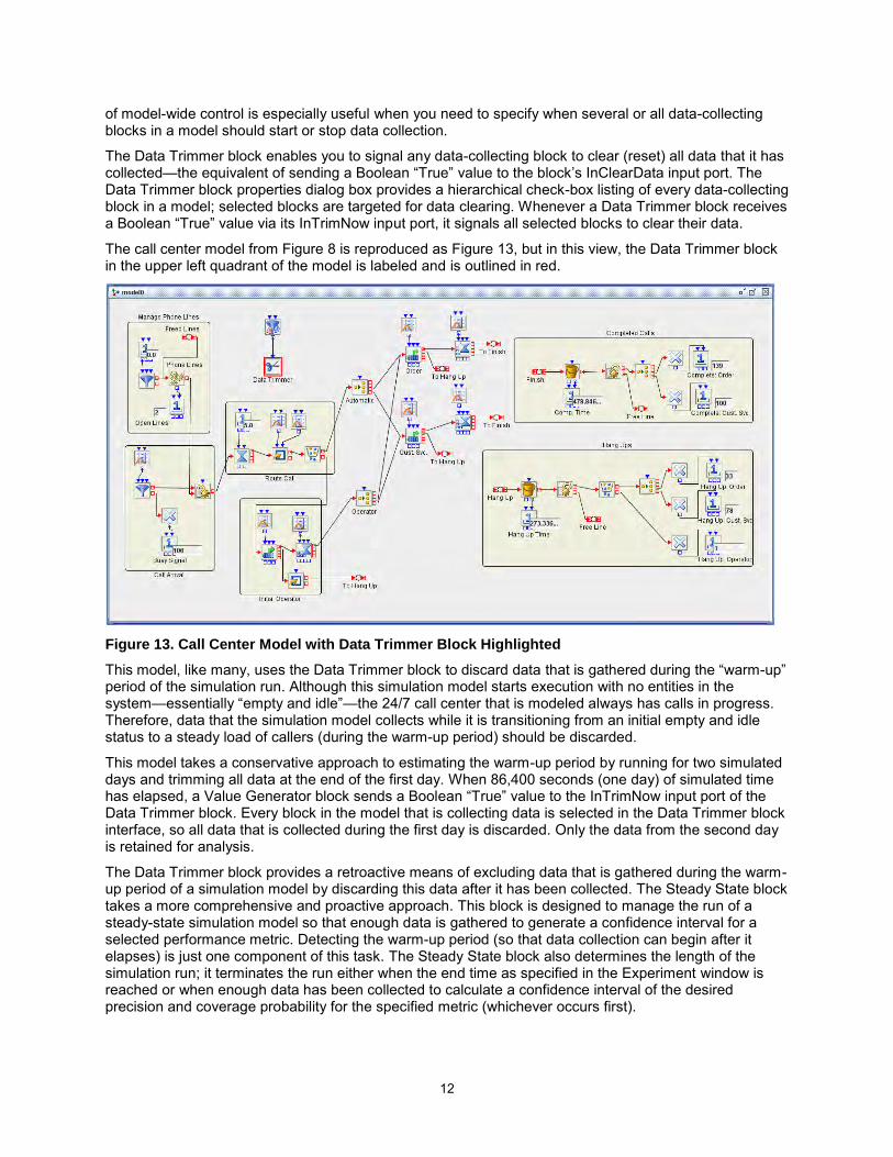
The call center model from Figure 8 is reproduced as Figure 13, but in this view, the Data Trimmer block in the upper left quadrant of the model is labeled and is outlined in red.

Figure 13. Call Center Model with Data Trimmer Block Highlighted

This model, like many, uses the Data Trimmer block to discard data that is gathered during the “warm-up” period of the simulation run. Although this simulation model starts execution with no entities in the system—essentially “empty and idle”—the 24/7 call center that is modeled always has calls in progress. Therefore, data that the simulation model collects while it is transitioning from an initial empty and idle status to a steady load of callers (during the warm-up period) should be discarded.

This model takes a conservative approach to estimating the warm-up period by running for two simulated days and trimming all data at the end of the first day. When 86,400 seconds (one day) of simulated time has elapsed, a Value Generator block sends a Boolean “True” value to the InTrimNow input port of the Data Trimmer block. Every block in the model that is collecting data is selected in the Data Trimmer block interface, so all data that is collected during the first day is discarded. Only the data from the second day is retained for analysis.

The Data Trimmer block provides a retroactive means of excluding data that is gathered during the warm-up period of a simulation model by discarding this data after it has been collected. The Steady State block takes a more comprehensive and proactive approach. This block is designed to manage the run of a steady-state simulation model so that enough data is gathered to generate a confidence interval for a selected performance metric. Detecting the warm-up period (so that data collection can begin after it elapses) is just one component of this task. The Steady State block also determines the length of the simulation run; it terminates the run either when the end time as specified in the Experiment window is reached or when enough data has been collected to calculate a confidence interval of the desired precision and coverage probability for the specified metric (whichever occurs first).

13

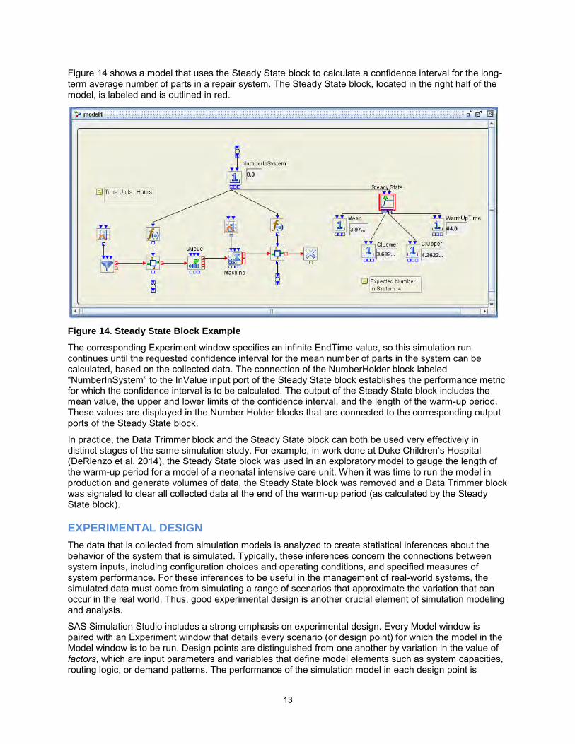
Figure 14 shows a model that uses the Steady State block to calculate a confidence interval for the long-term average number of parts in a repair system. The Steady State block, located in the right half of the model, is labeled and is outlined in red.

Figure 14. Steady State Block Example

The corresponding Experiment window specifies an infinite EndTime value, so this simulation run continues until the requested confidence interval for the mean number of parts in the system can be calculated, based on the collected data. The connection of the NumberHolder block labeled “NumberInSystem” to the InValue input port of the Steady State block establishes the performance metric for which the confidence interval is to be calculated. The output of the Steady State block includes the mean value, the upper and lower limits of the confidence interval, and the length of the warm-up period. These values are displayed in the Number Holder blocks that are connected to the corresponding output ports of the Steady State block.

In practice, the Data Trimmer block and the Steady State block can both be used very effectively in distinct stages of the same simulation study. For example, in work done at Duke Children’s Hospital (DeRienzo et al. 2014), the Steady State block was used in an exploratory model to gauge the length of the warm-up period for a model of a neonatal intensive care unit. When it was time to run the model in production and generate volumes of data, the Steady State block was removed and a Data Trimmer block was signaled to clear all collected data at the end of the warm-up period (as calculated by the Steady State block).

EXPERIMENTAL DESIGN

The data that is collected from simulation models is analyzed to create statistical inferences about the behavior of the system that is simulated. Typically, these inferences concern the connections between system inputs, including configuration choices and operating conditions, and specified measures of system performance. For these inferences to be useful in the management of real-world systems, the simulated data must come from simulating a range of scenarios that approximate the variation that can occur in the real world. Thus, good experimental design is another crucial element of simulation modeling and analysis.

SAS Simulation Studio includes a strong emphasis on experimental design. Every Model window is paired with an Experiment window that details every scenario (or design point) for which the model in the Model window is to be run. Design points are distinguished from one another by variation in the value of factors, which are input parameters and variables that define model elements such as system capacities, routing logic, or demand patterns. The performance of the simulation model in each design point is

14

tracked through responses, which are metrics like throughput, waiting time, and queue length that are generated directly from the operations of the model. Both factors and responses are defined in SAS Simulation Studio at the project level, so they can be used in any model in the project. Anchors in any such model connect factors and responses to specific elements of the model.

THE EXPERIMENT WINDOW

The Experiment window enables you to include the factors and responses that are of interest to you. It displays the different factor values that distinguish the various design points, and after the simulation model runs, it also displays the response values for each replication that was run for each design point. You can save the detailed results in the Experiment window as a SAS data set or JMP table for later analysis, and you can also submit it directly to JMP for immediate analysis (a JMP license is required).

Factors can take many forms, and they describe, for example, numeric parameters, paths to external input data sources, or a probability distribution that is to be sampled in the model. For a probability distribution, a factor can specify the entire distribution, including the type (normal, Poisson, and so on), or it can specify values for the parameters of a particular distribution type. Figure 15 shows part of an Experiment window for the call center model discussed earlier.

Figure 15. Experiment Window with Numeric Factors

Because the purpose of this model is to study the effects of variation in capacity on the call center’s performance, the factors (with yellow column headers) specify the number of telephone lines available and the number of operators on staff at three different stations. Responses (with pink column headers) count the number of successful and unsuccessful calls, along with the duration of each type of call. For each design point, the displayed value is the average among the five replications that were run.

Figure 16 shows an Experiment window that uses two factors to specify probability distributions.

Figure 16. Experiment Window with Factors Specifying Probability Distributions

These two factors specify distributions for two processing times in the corresponding model. The first processing time is known to be exponential, so the factor ExponentialMean specifies just the mean of an exponential distribution. The distribution of the second processing time is not as easily characterized, so the factor ProcessTime2 specifies both the type of the distribution and its associated parameters. Between the two design points, only the mean of the first distribution changes, but the second distribution changes from normal to uniform.

AUTOMATIC INTERACTIVE EXPERIMENTAL DESIGN WITH JMP

With SAS Simulation Studio, you can use design points to parameterize and control the execution of a simulation model in many ways. But as you might imagine, creating a set of design points that accurately represents the range of variations among possible operational scenarios for even a moderately complex simulated system is no trivial task. Fortunately, SAS Simulation Studio enables you to coordinate closely with JMP’s experimental design capabilities (a JMP license is required).

15

Even though creating individual design points manually is perfectly acceptable—and, in the case of narrowly targeted investigation of scenarios, preferable—JMP can provide valuable assistance in creating experimental designs. The result is more comprehensive designs that are quicker and far easier to complete than those that you create manually.

Figure 17 shows an Experiment window for the call center model discussed earlier. Factors and responses have been defined, anchored to specific elements of the model, and included in this Experiment window.

Figure 17. Initiating Automated Experimental Design with JMP

Currently no design points are defined. When the JMP server is running in the background, right-click in the Experiment window and select Make Design to create an experimental design with the JMP Custom Design platform. JMP creates the experimental design that is partially displayed in Figure 18.

Figure 18. Experimental Design Created with JMP

By default, JMP creates a main-effects screening (or optimal) design (SAS Institute Inc. 2017a). If you need to modify this design, you can open the Simulation Studio DOE window in JMP, make the necessary changes, and send the modified design back to SAS Simulation Studio. Figure 19 shows this window, with the user in the process of adding second-order interaction terms. After clicking Make Design to create a design that includes these interaction terms, the user would click Commit at the top of the window to send the modified design to SAS Simulation Studio for execution.

The Custom Design platform is not the only experimental design platform in JMP. To access other JMP experimental design platforms, follow the steps that are outlined in the section “Using Other JMP Design of Experiment Platforms” in “Appendix C: Design of Experiments,” in SAS Simulation Studio 14.3: User’s Guide (SAS Institute Inc. 2017b).

16

Figure 19. Modifying an Experimental Design

EXPERIMENTAL DESIGN WITH SAS

You can also write a SAS program to create an experimental design (SAS Institute Inc. 2017b). First, define your factors and responses and anchor them in your model. Include the factors and responses in an Experiment window. Ensure that your Experiment window contains at least one design point (by default, an Experiment window contains one design point), then right-click in the window and select Save Design to save its contents as a SAS data set.

Now you can use a SAS program to create an experimental design. Several procedures are available in SAS/STAT® (SAS Institute Inc. 2017d) and SAS/QC® (SAS Institute Inc. 2017c) software that you can use to create a design. This program uses PROC PLAN in SAS/STAT to create a full factorial design for a repair shop model with three factors that denote staffing levels at three stations in the model: proc plan seed=87654;

factors NumService=3 NumRepair=3 NumQC=3 / noprint;

output out=Project.Exp

NumService nvals=(1,2,3)

Numrepair nvals=(1,2,3)

NumQC nvals=(1,2,3);

run;

quit;

The output SAS data set, Exp.sas7bdat, in the library Project is the same SAS data set that was created when you saved the contents of the Experiment window, so the full factorial design that is created by PROC PLAN overwrites the original design. To import the new design into the Experiment window, right-click in the Experiment window, select Load Design, and navigate to the location of the newly created SAS data set. Figure 20 shows the Experiment window after you load the full factorial design.

17

Figure 20. Experimental Design Created Using SAS

INTEGRATING WITH OTHER ANALYTICS

Like any form of analytics, discrete-event simulation is never done in isolation. People who work in discrete-event simulation rarely focus solely in this area. Thus, integration between simulation and other analytics is essential. This paper has discussed how simulation uses descriptive and predictive input data, which is customarily produced by corresponding forms of analytics. In addition, output data that is produced by discrete-event simulation is almost universally subjected to formal or informal descriptive analysis. With SAS Simulation Studio, you have a unique ability to perform all such analyses within a unified framework, because SAS Simulation Studio is just one component of a broad spectrum of SAS analytic products and features.

The SAS Program block in SAS Simulation Studio provides even deeper integration with other SAS analytics because it enables you to execute a SAS program or a JMP script within your simulation model. The code that is specified by this block can be run automatically after all replications of all selected design points have executed, or the model can signal it to run (repeatedly, if necessary) via a Boolean “True” value sent to an input port on the block. The code can run on the same SAS client as SAS Simulation Studio or on a remote SAS workspace server (as specified by you in the Configuration dialog box).

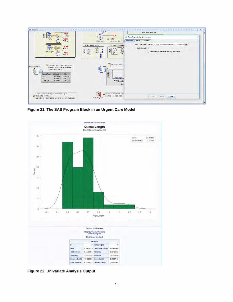
You can use the SAS Program block, for example, to preprocess input data for your model. You might need to reformat some data or synthesize several data sources before you use them in your model. You can also use this block to analyze simulated data. Figure 21 shows a partial view of a model of a walk-in urgent care medical facility. The SAS Program block is located at the bottom of the Model window and is outlined in red. The SAS Program block properties dialog box is expanded on the right side of the figure and indicates that the program “Generatereport_UCModel.sas” is to be run. Because the Auto Submit box is checked, the program runs at the end of the simulation model run. The program performs a statistical analysis of the data that the model collects by using PROC MEANS and PROC UNIVARIATE in Base SAS® software. Part of the output from the program appears in Figure 22. The program analyzes length and waiting times for the queues and utilization of the servers and the resources.

18

Figure 21. The SAS Program Block in an Urgent Care Model

Figure 22. Univariate Analysis Output

19

Instead of running the indicated SAS program or JMP script after the run of a simulation model concludes, you can trigger the SAS Program block to run the code during the simulation run. As mentioned before, you can use this feature to, for example, preprocess input data or perform other tasks that must be completed before the simulation model runs. You can also use the SAS Program block to run code that takes an active role in the internal logic of your model. For example, you can use this feature to periodically calculate an optimal production plan or update statistics that affect service goals.

Figure 23 shows a model of a pharmaceutical clinical trial. In the first phase, a new drug is tested on 50 patients for each of four proposed doses. When the first phase ends, an auxiliary entity flows through a Gate block that sends a Boolean “True” value to the InSubmitCode input port of a SAS Program block at the bottom of the Model window. The SAS program that is specified by this block executes a power and sample size calculation to determine how many additional patients should be tested at each dose so that the testing produces statistically significant results with sufficient probability (SAS Institute Inc. 2017d). This program calls PROC TTEST and PROC POWER in SAS/STAT.

Figure 23. Clinical Trial Model Using the SAS Program Block

CONCLUSION

Discrete-event simulation modeling with SAS Simulation Studio has always been notable for its power and flexibility. These traits are also reflected in its capabilities in data input, data use, output data creation, and experimental design, and in the ways in which it integrates with and incorporates other forms of analytics. The intuitive graphical user interface of SAS Simulation Studio offers you many options in building simulation models. This same freedom of choice extends well beyond simulation modeling, giving you great latitude in determining how your simulation work interacts with your overall analytic environment.

20

REFERENCES

Bélanger, Y., Couture, K., and Neusy, E. (2011). “An Application of SAS Simulation Studio: The Microsimulation of a Computer Assisted Telephone Interviewing System.” In Proceedings of the SAS Global Forum 2011 Conference. Cary, NC: SAS Institute Inc.

DeRienzo, C., Tanaka, D., Lada, E., and Meanor, P. (2014). “Creating a SimNICU: Using SAS Simulation Studio to Model Staffing Needs in Clinical Environments.” In Proceedings of the SAS Global Forum 2014 Conference. Cary, NC: SAS Institute Inc.

Hevener, G., Flinchum, T., and Lada, E. (2013). “Projecting Prison Populations with SAS Simulation Studio.” In Proceedings of the SAS Global Forum 2013 Conference. Cary, NC: SAS Institute Inc.

Hughes, E., and Lada, E. (2015). “Practical Applications of SAS Simulation Studio.” In Proceedings of the SAS Global Forum 2015 Conference. Cary, NC: SAS Institute Inc.

Hughes, E., Lada, E., Lopes, L., and Pólik, I. (2016). “Using SAS Simulation Studio to Test and Validate SAS/OR Optimization Models.” In Proceedings of the SAS Global Forum 2016 Conference. Cary, NC: SAS Institute Inc.

SAS Institute Inc. (2017a). JMP 13 Design of Experiments Guide. 2nd ed. Cary, NC: SAS Institute Inc.

SAS Institute Inc. (2017b). SAS Simulation Studio 14.3: User’s Guide. Cary, NC: SAS Institute Inc.

SAS Institute Inc. (2017c). SAS/QC 14.3 User’s Guide. Cary, NC: SAS Institute Inc.

SAS Institute Inc. (2017d). SAS/STAT 14.3 User’s Guide. Cary, NC: SAS Institute Inc.

Yi, J., Lada, E., Smith, A., and Gray, C. (2014). “Work Area Optimization at a Major European Utility Company.” In Proceedings of the SAS Global Forum 2014 Conference. Cary, NC: SAS Institute Inc.

ACKNOWLEDGMENTS

Emily Lada contributed very substantially to the content and form of this paper while she was a SAS employee. Emily is now a faculty member at Meredith College in Raleigh, NC.The author is grateful for her many valuable thoughts and suggestions.

CONTACT INFORMATION

Your comments and questions are valued and encouraged. Contact the author:

Ed Hughes SAS Institute Inc. Ed.Hughes@sas.com

SAS and all other SAS Institute Inc. product or service names are registered trademarks or trademarks of SAS Institute Inc. in the USA and other countries. ® indicates USA registration.

Other brand and product names are trademarks of their respective companies.