Long Run Relationships between Base Metals, Gold and Oil

Master Thesis Second Year

Masters of Science in Finance

Spring 2010

Authors

Supervisor

Garib Yusupov

Wenjia Duan

Karl Larsson

Department of Economics

ABSTRACT

This paper investigates the possible presence of long-run relationships (cointegration)

among base metals and between base metals, Crude oil and Gold, using the Johansen

multivariate approach and VEC Engle-Granger causality tests. The commodities used are

seven base metals: Aluminum, Aluminum Alloy, Copper, Nickel, Zink, and Tin (from the

London Metal Exchange), Crude oil and Gold. The Johansen approach results indicate that

Aluminum, Copper, Gold and Nickel share long-run relationships with each other. VEC

Granger Causality test at 10% significance level shows that all nine variables are cointegrated

with at least one of the remaining variables in the group which indicate the diversification

possibilities are limited. As for the price discovery, price development of Aluminum and

especially Copper should be given more attention, since they Granger-cause several of the

other variables.

Key Words: Johansen Cointegration Test, VEC Granger Causality, Weak Exogeneity, Commodities

ACKNOWLEDGEMENTS

The authors would like to thank Professor Hossein Asgharian, Professor David Edgerton and

our teacher in Time Series Analysis Ph.D Per Hjertstrand for their really helpful suggestions.

We especially thank our supervisor Ph.D Karl Larsson for his time, effort and constructive

criticism during the thesis work process.

TABLE OF CONTENTS

1. Introduction ...................................................................................................................................... 1

1.1 Purpose and Motivation .................................................................................................... 3

1.2 Outline of the Study ................................................................................................................... 3

2. Literature Review .............................................................................................................................. 4

3. Data ..................................................................................................................................................... 7

4. Methodology ....................................................................................................................................... 9

4.1 Stationarity ...................................................................................................................... 10

4.2 Stationarity and Unit Root Tests ........................................................................................... 11

4.3 Cointegration .................................................................................................................. 13

4.3.1 Error Correction Model ................................................................................................................. 14

4.3.2 Engle-Granger (EG) Univariate Cointegration Test and Parameter Estimation Method .... 15

4.3.2.1 Limitations of the Engle-Granger Approach ................................................................. 17

4.3.3 Johansen Multivariate Cointegration Test .................................................................................. 17

4.3.3.1 Determining the number of cointegrating vectors in Johansen Approach ................ 19

4.3.3.2 Specifying of the Vector Error Correction Model.......................................................... 20

4.3.4 Weak Exogeneity and Conditional VECM ........................................................................................ 22

4.3.4.1 Limitations of The Johansen Approach .......................................................................... 24

4.3.5 Vector Error Correction Granger-Causality Test ............................................................................... 25

4.3.5.1 Bottom Up Approach ......................................................................................................... 25

4.3.5.2 Top down Approach .......................................................................................................... 26

5. Empirical Results and Analysis ...................................................................................................... 28

5.1 Integration: Unit root tests and stationarity test results .................................................. 28

5.2 Cointegration: Johansen test results ............................................................................... 29

5.3 Tests for the Separate Models ........................................................................................ 31

5.3.1 Tests Results for Aluminum and Aluminum Alloy .................................................................. 32

5.3.2 Tests Results for the Eight-Variable Group ............................................................................... 32

6. Limitations of the Study and Suggestions for Further Research ................................................ 36

7. Conclusion ........................................................................................................................................ 37

8. References ......................................................................................................................................... 38

9. Appendix........................................................................................................................................... 42

1

1. Introduction

In July 2007 prices on three groups of commodities (crude oil, gold, and base metals)

decreases, with the common factor being rallying US dollar, and an article in London South

East discusses the possible relationship. Harvey (2007), the author of the article, points out

that oil and gold rather often move closely together over time. Also gold and base metals

seem to have a long-term relationship, even though it may be weaker than in the case of oil

and gold.

On the 5th of Feb, 2010 one can read in Financial Times that prices on gold, base metals

and oil all have gone down (Flood, C., 2010). This time the cause named is worries in the

sovereign debt market.

What is the price relationship between oil and base metals? On the one hand, during the

expansion phase in a business cycle, both oil prices and metal prices should rise due to

increase in demand for both. On the other hand, it is known that high oil prices have a

depressing effect on general business activity and there is strong evidence that too high oil

prices may be causing recessions (Engemann et al., 2010).

What price links do exist between oil and gold? On the one hand, when inflation

increases and energy prices go up, so does the gold price, as it is used to hedge off the effect.

On the other hand, in times of high volatility demand for oil plunge and its price goes down,

whereas gold price goes up as the precious metal is seen as "safe heaven" investment

(Durrant, 2007). But gold has competitors in that role, not least government bonds. Thus the

positive relationship between oil price and gold price could persist even in times of high

market volatility, according to Peter Fertig, an analyst at Dresdner Kleinwort and cited in

London South East in July 2007.

When it comes to possible long-term relationships between gold and industrial metals it

may be necessary to remember in what areas gold is used. The precious metal is not merely a

vehicle for wealth conservation and input for jewelry production. In fact, Goldipedia (2010)

lists a range of areas where gold is used due to its numerous valuable properties: electronics,

space & aeronotics, medical, cleantech /environmental, nanotechnology, dentistry, decorative,

engineering, food & drink; beauty. It is suggested that recently the industrial demand for gold

has been a major factor in driving the gold price up (Ibid.). Therefore, we think there could

2

potentially be a cointegrating relationship between industrial metals prices and the gold price

during bull markets. The relationship could be there during bear markets as well. According

to Michael Widmer, an analyst at Clayton, price decrease for commodities is generally

followed by price decrease for gold, as many investors prefer to hold cash (Harvey, J., 2007).

The three commodity groups’ price movements seem to have at least short term

relationships, as the variables exhibit positive correlations both in levels and in returns (see

Appendix B-G, Table 1-6). So, is it a “normal” behavior for the three type of commodities to

move together, i.e. do they have a long-term relationship, or are these just temporary co-

movements? With this paper we aim to find that out using cointegration analysis.

We use 15-year daily closing prices, acquired from DataStream, for base metals traded

on London Metal Exchange, for gold, traded on London Bullion Market Association, and for

Brent Crude oil, traded on electronic Intercontinental Exchange.

Studies of long-run relationships between non-stationary variables have been greatly

facilitated by the introduction of the notion of cointegration and a testing method by Clive

Granger and Robert Engle in the 1980s. The two famous econometricians show that two time

series, both containing a unit root, share a long-term relationship, i.e. are cointegrated, if a

linear combination of the two is stationary. This enables researches to discriminate between

spurious and meaningful regressions. It allows econometricians to utilize the information

contained in levels, which previously was lost due to the, until that time, common procedure

of conducting studies on first-differenced data and thus retaining only short-term information

in the time series.

Although the Engle-Granger methodology from 1987 for detecting cointegration and

estimating the parameters has become very popular, it has a number of deficiencies.

Therefore, for this study we have chosen to mainly use the Johansen multivariate method to

test the data for cointegration, and VEC Granger-causality test to determine potential lead-lag

regularities.

3

1.1 Purpose and Motivation

This paper studies the possible presence of long-run relationship(s) among base metals,

as well as between base metals, gold and oil. In the presence of the long-run relationships, the

causality in the relationships for the commodities is investigated.

For an investor the results of the study concerning the possible presence of long-run

relationships should be of interest as they indicate whether there are long-term diversification

benefits in being active in all three markets. And identification of stable lead-lag relationships

could provide the investor with some ability to “predict” future. We were not able to find

studies similar to this, and therefore we wish to fill some of the gap with our little

contribution.

1.2 Outline of the Study

The rest of this paper is organized as follows: Section 2 presents a brief review of

relevant previous studies. In section 3 we describe the data we use for the study. In section 4

we explain our methodology. Section 5 presents the empirical results and analysis and Section

6 illustrates the limitation of the study and our suggestion for further research. The last section

concludes the paper.

4

2. Literature Review

Few existing studies look into cointegration and lead lag relationship between crude oil,

gold and base metals. The studies, we have come across, have a focus that is either narrower

or wider, compared to our study. Some of the researchers choose to investigate potential long-

run relationship between spot price and some financial instrument(s) with the same

underlying asset. Other researchers look for cointegration between some asset(s), and

macroeconomic factors.

Watkins and McAleer (2002) examine the long term relationship between copper

futures and spot price based on the risk premium hypothesis and the theory of storage. They

extend the previous research to take unit root and non-stationarity into account. Johansen

cointegration approach with the adjusted empirical model is utilized with daily data for spot

and 3-month contract settlement price of copper from the 3d of Jan 1989 to the 30th of Sep

1998 obtained from the London Market Exchange. Moreover, since the contracts on LME are

denominated in US Dollars, the data also includes the US dollar 3-month Treasury bill

secondary market rate as interest rate to detect the macroeconomic effect. The results indicate

that there exists long run correlation with the full sample set while only two out of the three

sub-sample sets have this relationship if considering the structural break. This study focuses

on the cointegration relationships between financial instruments on the same underlying

whereas we are interested in the cointegration relationships between different commodities.

Sari et al (2010) use both Johansen methods and Pesaran’s bounds testing approach to

check for cointegration between the spot prices for oil, precious metals, and exchange rate. In

the test, daily data of closing spot price for 4 commodities (gold, silver, platinum and

palladium), oil spot price and USD/euro exchange rate with the period from the 1st of Apr

1999 to 19th Sep 2007 is used. All series are modeled in natural logarithms. Dummy variables

are also considered for establishment of the oil price band by Organization of the Petroleum

Exporting Countries (OPEC) in 2000, the 9/11 New York City attack and the 2003 Iraq war.

Before testing the data, they use the forecast error variance decomposition (VDC) and

generalized impulse response approaches to understand the impacts and reaction to shocks.

The results from bounds test suggest that there is no cointegration among the precious metals

spot price, oil prices and the exchange rate although they have strong correlations in the short

5

run. JJ test confirms the results that there is no long run equilibrium relationship between the

spot price returns and changes in the exchange rate. The authors conclude that the tested

commodities may be not sensitive to common macroeconomic factors in the long-run but that

the precious metal’s spot prices and exchange rate may be closely related in the short run after

shocks occur. In our study, instead of using exchange rate or other macroeconomic factors,

base metals are used.

Testing and detecting cointegrating relationships between financial assets can not

provide sufficient information to investors for their hedging strategies. Therefore, lead-lag

relationships of the commodities need to be investigated. Many researchers have studied this

issue, but often the researchers focus on cointegration between financial instruments on the

same underlying asset.

Garbade and Silber (1983) point out that futures markets perform the function of price

discovery which indicates that futures price lead the spot price. The following researchers

apply this Garbade-Silber Model on various commodities. Silvapulle and Moosa (1999) test

the crude oil market and confirm Garbade-Silber’s discovery. They argue that because of the

lower transaction cost and convenience of shorting, futures price responds to new information

much more quickly than the spot price. Asche and Guttormsen (2002) also try to find out

whether there is a lead-lag relationship between spot and futures prices for gas oil with the

improvement of using the Johansen test in the multivariate framework. Monthly data from

Apr 1981 to Sep 2001 with the futures contracts maturing in 1, 3 and 6 months are used. After

affirming the time series are cointegrated, exogeneity test is utilized for the causality

relationships. Empirical results indicate that futures price leads the spot price and it plays a

price discovering role. Besides, futures contacts with longer maturity lead those with shorter

maturity. In our study, we are more interested in finding out whether some commodities are

performing that price discovery function towards other commodities in the system.

Nevertheless, limited researches have been conducted to explore the relationship

between crude oil, base metals and gold. Cashin et al (1999) test the correlations between

seven seemingly-unrelated commodities: wheat, copper, crude oil, gold, lumber and cocoa;

with the time period from April 1960 to November 1985. Empirical results demonstrate that

there exist significant correlations. The analysis is implemented using a longer time period,

from Jan 1957 to July 1999, and the results display that crude oil and gold have significant

6

harmony in prices. Nonetheless, their study can not find whether these commodities’ prices

move together. In our study we partly replicate the research with newer data, since we only

test crude oil, gold, copper and several other base metals for cointegration during the period

1995-2010.

Baffes (2007) examines the price effect of crude oil on some other commodities. One of

the results is that aluminum has almost zero elasticity. That happens maybe due to the fact

that electricity and natural gas markets, which aluminum production is subjected to, are local,

thus not responsive to global energy demand and supply conditions. The unresponsiveness of

copper, nickel, and zinc prices to the price of crude oil is mainly due to the long term

negotiated price between extraction companies and governments of the countries where the

resource is extracted. On the contrary, iron and tin have highly significant estimate, probably

due to high costs, e.g. transportation cost, and Tin Agreement, respectively. The author

assumes from the beginning that it is crude oil which is affecting other commodities. We do

not assume anything and allow for the possibility that other commodities may influence the

crude oil price.

Most of the studies we have mentioned above focus narrowly on finding the relationship

between the spot and derivatives prices with the same underlying assets or assets spot prices

and some macroeconomics factors, such as interest rates and exchange rates. To the best of

our knowledge, the research of base metals, crude oil and gold has not been conducted before.

Therefore with this study we aim to contribute to the field of research on issues of

cointegration between commodities: Crude Oil, Gold, Aluminum, Aluminum Alloy, Lead,

Copper, Tin, Zinc and Nickel.

7

3. Data

Commodities studied in this report are Aluminum, Aluminum Alloy, Copper, Lead,

Nickel, Tin, Zinc, Crude Oil and Gold. Daily data on these commodities’ spot prices cover a

15-year period, from the 7th of April 1995 to the 7th of April 2010, and is obtained from

DataStream. Each time series contains 3914 observations. Silver is excluded mainly due to

the lack of data for the time period. Besides, Ciner (2001)’s study finds that gold and silver do

not have long run relationship which is also consistent with the findings by Escribano and

Granger in 1998.

The metal prices except gold are retrieved from London Metal Exchange (LME)1 which

is the world’s premier non-ferrous metals market located in London. Gold price is obtained

from London Bullion Market (LBM)2. Prices quoted by the LME prior to July 1993 are

denominated in British Pounds while after that in US dollars. Considering the time period in

this report, all the commodities are traded in US dollars3. Brent crude oil was originally traded

on the open-outcry International Petroleum Exchange in London, but since 2005 has been

traded on the electronic Intercontinental Exchange, known as ICE.

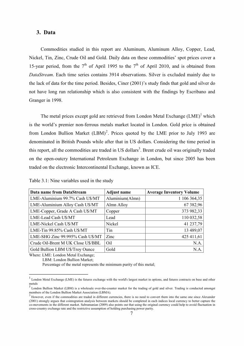
Table 3.1: Nine variables used in the study

Data name from DataStream Adjust name Average Inventory Volume LME-Aluminium 99.7% Cash U$/MT Aluminium(Almn) 1 106 364,35 LME-Aluminium Alloy Cash U$/MT Almn Alloy 67 382,96 LME-Copper, Grade A Cash U$/MT Copper 373 982,33 LME-Lead Cash U$/MT Lead 110 032,58 LME-Nickel Cash U$/MT Nickel 41 237,79 LME-Tin 99.85% Cash U$/MT Tin 13 489,07 LME-SHG Zinc 99.995% Cash U$/MT Zinc 425 411,61 Crude Oil-Brent M UK Close U$/BBL Oil N.A. Gold Bullion LBM U$/Troy Ounce Gold N.A.

Where: LME: London Metal Exchange; LBM: London Bullion Market; Percentage of the metal represents the minimum purity of this metal;

1 London Metal Exchange (LME) is the futures exchange with the world's largest market in options, and futures contracts on base and other metals 2 London Bullion Market (LBM) is a wholesale over-the-counter market for the trading of gold and silver. Trading is conducted amongst members of the London Bullion Market Association (LBMA). 3 However, even if the commodities are traded in different currencies, there is no need to convert them into the same one since Alexander (2001) strongly argues that cointegration analysis between markets should be completed in each indices local currency to better capture the co-movements in the different market. Subramanian (2009) also points out that using the original currency could help to avoid fluctuation in cross-country exchange rate and the restrictive assumption of holding purchasing power parity.

8

Cash U$: Spot price traded in US dollars; SHG: Super high grade; MT: Metric Ton; BBL: the abbreviation of and oil barrel; N.A.: not available.

Figure 3.1 plots the movement of the commodities’ spot price during the 15-year period.

The data used in this study is in natural logs. (See Appendix A Figure 1)

The descriptive statistics of all logged and raw data as well as log returns and their

correlations are presented in Appendix B-G Table 1-6. The tables show that all of the

commodities have positive correlation with each other which means diversification benefits in

the short run are limited.

Figure 3.1 Commodities’ spot price from 7th April 1995 to 7th April 2010

Note: AlmnUSD/10 MT and AlmnAlUSD/10 MT represent the price of Aluminum per 10 MT and the price of Aluminum Alloy per 10 MT, respectively;

CoppUSD/MT represents the price of copper per MT; LeadUSD/10 MT represents the price of Lead per 10 MT; NicUSD/MT and TinUSD/MT represents price for Nickel and Tin per MT, respectively; ZincUSD/10 MT is the price of Zinc per 10 MT; OilBREUSD/100 BBL is the price for Crude oil per 100 oil barrel; GoldUSD/20 TO represents the price of gold per 20 troy ounce.

0

10000

20000

30000

40000

50000

60000

AlmnUSD/10 MT

AlmnAlUSD/10 MT

CoppUSD/MT

LeadUSD/10 MT

NicUSD/MT

TinUSD/MT

ZincUSD/10 MT

OilBREUSD/100 BBL

GoldUSD/20 TO

9

4. Methodology

To answer the question of this paper, we adopt the following strategy. We start by

testing the variables for non-stationarity. A necessary condition for cointegration between the

variables is that the variables are non-stationary, i.e. integrated of order higher than zero. We

conduct confirmatory data analysis by utilizing both unit root tests (Augmented Dickey-Fuller

(ADF) test, Phillips–Perron (PP) test) and a stationarity test (Kwiatkowski-Phillips-Schmidt-

Shin (KPSS) test). We proceed with the test procedures for cointegration. Our main method is

the Johansen multivariate methodology based on Vector Autoregression (VAR). Akaike

information criteria (AIC) is used to determine the lag length in the VAR. Next, the reduced

rank regression is run on three different Vector Error Correction (VEC) models. The

difference between the models is the deterministic components, i.e. a constant and trend.

Applying the Pantula Principle, the optimal VEC model as well as the rank (the number of

cointegrating vectors) is determined and two cointegrating vectors are obtained. Without

strong economic theory to be used as a guide for identifying restrictions later on, Aluminum

Alloy is excluded. The logic behind the decision is that Aluminum and Aluminum Alloy are

probably strongly cointegrated. Both the Engle-Granger cointegration test and the Johansen

test confirm our guess. The Granger-causality test shows a bi-directional cointegrating

relationship. The reason that Aluminum Alloy is skipped but not Aluminum is their respective

average inventory volume difference (see Table 3.1). The previous steps of the Johansen

methodology are repeated on the eight variables left. The eight variables in the unrestricted

Vector Error Correction Model (VECM) selected are then tested for weak exogeneity

(restrictions on α) by imposing joint restrictions on the speed of adjustment coefficients vector

α and the cointegrating coefficients vector β. The directions of the cointegrating relationships

detected in the Johansen approach for both unrestricted and conditional models are examined

with VEC Granger-causality test. Below, both the relevance of the methodology and the

practical implementation are presented in more detail.

10

4.1 Stationarity

Before applying the cointegration test, it is necessary to test whether the time series are

stationary. The weak form of stationarity, which is the most commonly used form for

practical reasons, is present when a time series has a constant mean, a constant variance and a

constant autocovariance:

����� � � (4.1)

����� ��� � � �� (4.2)

����� ����� �� � �����, for all t2-t1 (4.3)

A time series, consequently, is non-stationary if any of the conditions is violated, i.e. its

mean, variance and covariance are time depending.

Stationary and non-stationary time series have greatly different behaviors and

properties. In a stationary process a “shock” at time t has a diminishing influence on the

system as time goes by, i.e. lower effect at t+1, even lower at t+2, etc., and gradually dies

away. In contrast, in a non-stationary process the effect of a “shock” always persists infinitely

into the future without losing its strength.

Application of standard regression techniques on economically unrelated non-stationary

time series data can result in Spurious, or Nonsense, Regressions. Regressing one non-

stationary time series on a different unrelated non-stationary time series can give high R2 and

significant coefficient estimates, simply because both series are trending over time, even

though there is no real long-term relationship between the series.

Standard assumptions on asymptotic analysis are not valid in a regression model that is

based on non-stationary time series, i.e. the t-statistic, F-statistic, etc. do not follow their

respective distributions.

Among different non-stationary models, one that is frequently used and of interest for

this paper is the random walk model with drift, also known as stochastic non-stationarity with

stochastic trend in the data:

�� � � ������ � �� (4.4)

11

where �� is a white noise disturbance term.

The expression in (4.4) can be generalized to an autoregression model with one lag

(AR(1)):

�� � � ������� � �� (4.5)

If φ =1, then the equation (4.5) is reduced to equation (4.4) which means that the time

series is non-stationary. In this case yt is equal to the sum of all the “shocks” up to time t plus

an initial value of y at time 0:

�� � �� � � ������� , t → ∞. (4.6)�This type of process is also called a unit root process, because the characteristic

equation for this process has the root of one4. In order to make this non-stationary time series

stationary one needs to difference (4.4) once:

�� ���� � � ������ ���� � �� � � � �� (4.7)

This type of a non-stationary time-series is therefore known as difference - stationary,

since the method to use to make it stationary is to difference it. (Brooks, 2008)

4.2 Stationarity and Unit Root Tests

Because of the large differences in the properties of stationary and non-stationary time

series, it is important to check the data one uses for stationarity. The three most commonly

used tests to decide whether a time series is stationary or non-stationary are the Augmented

Dickey-Fuller test (ADF-test), Phillipls-Perron's test (PP-test), and Kwiatkowski-Phillips-

Schmidt-Shin test (KPSS-test). The three tests are hypothesis tests, but the first two tests are

unit root tests and the third one, KPSS-test, is a stationarity test. ADF test and PP test have the

null hypothesis that the time series is integrated of order one, usually denoted I(1), against the

4 Theoretically, it is possible that φ >1, but this case is usually ignored as it does not describe many financial or economic time series. The case of φ >1 is also intuitively unappealing as it would mean that a “shock” at time t increases its effect into the future, instead of fading away.

12

alternative hypothesis, that the series is stationary, denoted I(0). The KPSS test switches the

hypotheses and has as the null hypothesis that the time series is stationary.

Consider the following autoregression model, which can also include a constant term

and a trend term:

��� � ������ � � ������ ����� �� ��� ����� � ��� (4.8)

where ∆yt = yt - yt-1, and ψ = φ – 1.

The ADF method tests the following hypothesis:

H0: ψ = 0, the time series has a unit root, i.e. it is non-stationary.

H1: ψ < 0, the time series does not have a unit root, i.e. it is stationary.

The lags in equation (4.8) are included in order to capture all dynamic structure in the

endogenous variable and thus make certain that the residual term ut is not autocorrelated (the

residuals have to be white noise in order for this test to be valid). It is therefore important to

decide on the number of lags to include. One way to decide on the number of lags to be

included in the equation is by choosing the number of lags that minimizes the Akaike

Information Criteria (AIC) or the Schwarz Information Criteria.

The test statistic ( ψ!"#$��ψ!� )5 of the ADF-test follows a non-standard distribution, Dickey-

Fuller distribution, and not the normal t-distribution.

The PP test is similar to the ADF test with that difference that is allows the residuals to

be autocorrelated. Therefore the ADF test and the PP test often give similar results and share

pretty much the same weaknesses.

The major issue with the two tests is that they have a very low power to distinguish

between a unit root process and a process that is close to unit root but nevertheless is

stationary. This problem is more prominent if the sample is small. The reason the problem is

present is that the null hypothesis can not be rejected in two cases. The first one is if the

process is indeed non-stationary and the second one is if there is not enough information.

5 %&$��ψ!� is the estimated standard error of ψ.

13

One way to mitigate the problem is by conducting a confirmatory data analysis, which

means that one utilizes a stationarity test as a complement to the unit test(s) used. One such

test is the KPSS test. As mentioned before, the KPSS has switched the hypotheses:

H0: the time series does not have a unit root, i.e. it is stationary

H1: the time series has a unit root, i.e. it is non-stationary. (Brooks, 2008)

Ideally, the three tests should give results consistent with each other, i.e. if a time series

contains a unit root, then the ADF and PP- tests should accept the null, and the KPSS-test

should reject the null. If the results of the unit root test are contradicting to that of the

stationarity test, then either additional tests are needed or a choice has to be made. Harris and

Sollis (2005) suggest that in an unclear situation, the unit root test results should be preferred,

because of the consequences (see section 4.1) of a unit root in time series.

4.3 Cointegration

A problem one usually faces when using non-stationary variables, that have no real

relationship with each other, is that one can get regressions that “look” good ( high R2, highly

significant coefficients), but actually are meaningless. However, obviously, not all integrated

variables lack real relationships with each other. Many financial variables move closely

together in the long-term, as they are influenced by the same market forces or influence each

other. Stock prices and their options prices, spot prices and futures prices or other similar time

series, for example, can be expected to move together in the long-run, as they have the same

underlying or otherwise are connected. Thus, such variables can be cointegrated, meaning that

even though the time series in question are non-stationary, they can trend over time in a

similar fashion and therefore difference between them can be expected to be constant (Harris

& Sollis, 2003). Thus, non-stationary time series that exhibit a long-term equilibrium

relationship are said to be cointegrated. The possibility of non-stationary time series to be

cointegrated was first considered in 1970’s by Engle and Granger. They define cointegrated

variables in their paper from 1987 in the following way.

14

Consider two non-stationary time series, yt and xt where each of the time series become

stationary after differencing once, i.e. they are both integrated of order one, I(1). These non-

stationary time series are then said to be cointegrated of order one-one, CI(1,1) if there exists

a cointegrating vector α that in a linear combination of the two variables yields a stationary

disturbance term µt ~ I(0), in the regression µt� �� yt� -� αxt. Cointegration means that these non-

stationary variables share a long run relationship, and thus the new time series from

combining the related non-stationary time series is stationary, i.e. the deviations have finite

variance and a constant mean. Note that non-stationary variables can also have a non-linear

cointegrating relationship(s), but that is outside the scope of this paper.

In general, two series are cointegrated if they are both integrated of order d, I(d) and a

linear combination of them has a lower order of integration, (d-b), where b>0. Time series

have to be non-stationary for them to be able to be cointegrated. Thus, one stationary variable

and one non-stationary variable cannot have a long-term co-movement, as the first one has a

constant mean and finite variance, whereas the second one does not, so the gap between the

two will not be stationary. But, if there are more than two time series in a system, it is

possible for them to have different order of integration. Consider three time series, yt ~ I(2), xt

~ I(2), qt ~ I(1). If yt and xt are cointegrated, so that their linear combination results in a

disturbance term µt = yt - αxt which is integrated of order 1, I(1), then it is potentially possible

that ut and qt are cointegrated with resulting stationary disturbance term st��� qt� -� βut., where

α,β are cointegrating vectors. In general, with n integrated variables there can potentially exist

up to n-1 cointegrating vectors.

4.3.1 Error Correction Model

Engle and Granger (1987) show that if two variables are cointegrated then there must

exist an Error Correction Model (ECM) and vice versa. An error correction model, also

called an equilibrium correction model, is a model belonging to a class of dynamic models

that can be used to estimate a long-run relationship between cointegrated variables. The

model includes a combination of lagged values, as well as first differences of the variables

being tested:

1�� � 2��3� � 2����� �3���� � �� � (4.9)

15

where �3� = 3� – 3���

An error correction model includes both short-run and long-run effects that determine

how the dependent variable evolves over time. The term (yt-1 – γxt-1) in the error correction

model above is called error correction term and is stationary, if xt and yt are cointegrated with

the cointegrating coefficient γ. This term is equal to zero when the system of the two variables

is in its long-term equilibrium, otherwise it is different from zero and measures the distance

from equilibrium at time t (Harris and Sollis, 2003). The parameter β2 then measures how fast

the endogenous variable yt adjusts back to equilibrium. Thus, in an ECM yt reacts to changes

in the explanatory variable, ∆xt, between time t-1 and t, and to the disequilibrium between

itself and xt in time t-1. If the theory behind the possible cointegrating relationship of the

variables suggests it, one can insert a constant term in the error correction model, error

correction term, or both, thus the model can be modified as:

��� � 2� ��2��3� � 2����� � �3���� � ��� (4.10)

An error correction model can also be extended to include more variables than just two.

With three variables, xt, yt, and qt an error correction model can look like this, if no constants

are included:

��� � 2��3� � 2�4� � 25����� ��3��� �4���� � �� (4.11)

Another useful feature of an ECM is that all the components included in it are

stationary, allowing a valid application of standard statistical methods and procedures, eg.

OLS.

4.3.2 Engle-Granger (EG) Univariate Cointegration Test and Parameter Estimation Method

In 1987, Engle and Granger proposed a two-step modeling strategy when dealing with

non-stationary and possibly cointegrated panel data. The method is a residual-based

univariate, or single equation, process for estimating cointegration parameters. The logic of

the approach is intuitive, straightforward and easy to apply. Before applying the method, it is

necessary to make sure that the time series contain one unit root, because time series need to

be integrated to be able to be cointegrated.

16

In the first step a cointegrating regression is run using OLS in order to obtain the

parameter values, although no inference can be conducted on the coefficients. A simple static

model can be used:

��� � 6 � 23� � �� (4.12)

The residuals are then saved and tested for stationarity. ADF test can be applied on the

autoregression model:

�7� � 8�7��� � 9: (4.13)

where the error term υt ~ IID.

Because the test is applied on the residuals and not on the raw data, one cannot use the

critical values from the ADF test. Instead one uses the critical values tabulated by Engle and

Granger in 19876. If the u7 � is stationary, then according to the definition, the time series are

cointegrated. One can thus proceed to the second part of the method. But if the error term is

not stationary then the model needs to be estimated on the first differences instead of the

levels.

The second stage estimates the cointegration parameters as the residuals term is put as

an explanatory variable into the error correction model, for example of the following simple

short-run form:

��� � 2�3� � 2�7��� � 9: (4.14)

Where �7��� � ���� �;<�3���. By combining the non-stationary variables in this manner

this linear stationary relationship, also known as the cointegrating vector, can be obtained. In

this particular case our cointegrating vector is [1-;< ]. (Brooks, 2008).

The EG method is popular due to several reasons. The approach is simple in execution,

as it is easy to run OLS on the cointegrating equation and then run unit root tests on the

residuals term. Moreover, the ECM model in the second step can be extended into a general

dynamic form by including a larger number of lags of either one or both cointegrated

variables, yt and xt. Furthermore, since all variables in (4.14) are stationary, application of

6 later, Engle and MacKinnon (1991) presented a way of calculating critical values for the ADF unit root test on the residuals, which we are using in this study

17

standard statistical tests, such as t-test or F-test, is possible in order to be able to make valid

inference about β1 and β2.

4.3.2.1 Limitations of the Engle-Granger Approach

However, there are some limitations to the EG two-step method. 1. The approach is a

single-equation method and thus allows only one cointegrating relationship, although

hypothetically n-1 cointegrating vectors can exist among n non-stationary variables. 2. When

it comes to finite samples, this approach suffers from lack of power, both at the first stage

(testing for unit root) and the second stage (testing for cointegration). 3. Also, due to this

problem changing the roles of the variables would lead to different conclusions. 4. Moreover,

it can suffer from simultaneous equations bias. Two non-stationary variables are treated

asymmetrically, because one has to be defined as exogenous and the other one as endogenous,

even though the causal relationship can be going both directions simultaneously. 5.

Furthermore, because of the sequential construction of this approach misspecifications in the

first phase migrate into the second one. 6. Finally, the approach is not applicable when one

wants to test hypotheses concerning the actual cointegrating relationship defined in the long-

run regression equation in the first phase.

The most serious problem among them is the last one, as the first five problems are

expected to disappear asymptotically. To avoid the problems of the EG test, the Johansen

multivariate procedure, which is based on estimation of VAR systems, is applied.

4.3.3 Johansen Multivariate Cointegration Test

Johansen method extends the EG univariate method to a multivariate version. The non-

stationary, I(1), variables being tested for cointegration together form an autoregressive vector

(VAR), e.g. if we have three variables in a vector zt = [y1t,y2t,xt]´and all three variables are

assumed to be endogenous:

�=� ��>�=��� �?� >@=��@ � A���, ut ~ IN(0, Σ). (4.15)

where A an (n x n) matrix of parameters.

18

An important issue constructing the VAR is the number of lags to be included in the

model, so that we get Gaussian residuals in the error correction model later on. An often used

way to solve the problem is to use the Akaike information criteria when deciding on the

number of lags.

The univariate error correction model in (4.9) can be readjusted to the multivariate

framework as well and becomes a vector error correction model (VECM):

�=� � B�=��� �?� B@��=��@C� �D=��@ � A� (4.16)

where Π = -(I-A1- ...- Ak) and Γi = - (I-A1 - ... - Ai) (I = 1,...k-1). Π is a (3x3) matrix with

long-run information content, as Π = αβ´. α gives us the speed of adjustment to

disequilibrium, whereas matrix β contains long-run coefficients.

With two lags the full model looks as follows:

EF���F��F�5�E � � EF�����F����F�5���E � E��� ���� ��5� �5E G H

2�� 2� 25�2� 2 25H G E����������5���E (4.17)

In this multivariate model the error correction term, or cointegrating

relationship, contains up to n-1 vectors and is represented by β'*zt-1, which in turn is

embedded in Πzt-k in equation (4.16). Πzt-k has to be stationary in order for the residuals term

ut to be "white noise". This is possible in three cases:

1. All variables in zt are actually stationary, and not I(1) as assumed, i.e. Π has full rank;

2. The variables are non-stationary, but lack a long-run relationship with each other, i.e.

Π has zero rank;

3. There are up to (n-1) cointegrating relationships, i.e. Π has reduced rank.

Because we are dealing with non-stationary variables and are looking for cointegration,

only the third case is interesting for us. In the third case r� ≤� �n-1� stationary cointegration

vectors and (n-r) non-stationary vectors exist in β. But only the cointegration vectors will be

present in (4.16), in order for Πzt-k to be stationary, which in turn implies that (n-r) columns

in α are effectively equal to zero. Therefore in Johansen test one is interested in finding the

19

rank of Π. In 1988 Johansen proposed a maximum likelihood method for estimating α and β

which is called reduced rank regression. Expression (4.16) can be rewritten as follows:

�=� � MNO=P�Q � B�F=��� �?� B@��F=��@C� � A� (4.18)

Next, the effects of short-run dynamics are removed from (4.18) by separately

regressing the right-hand side of (4.18) and two vectors of residual terms are obtained, R0t and

Rkt:

1R� � S�1R��� � S1R�� �?� S@��1R���@C�� � T�� (4.19)

R��@ � U�1R��� � U1R�� �?� U@��1R���@C�� � T@� (4.20)

The two vectors of the residuals are then used to form residual matrices:

V�W � U�X� T��T@�YUZ�X �� i,j = 0, k (4.21)

Finally, we solve the equation:

[\V@@ V]^V^]V^^ [ � _ (4.22)

and obtain eigenvalues, a1> a2 > a 3>…> an , with corresponding eigenvectors

bc � ��d!1,…,�d!n ]. The largest eigenvectors up to r give us the maximum likelihood

estimate of β, β = ��d!1,…,�d!r ]. The estimated β and levels of zt deliver combinations with high

correlation with the stationary parts in (4.16), i.e. ∆zt terms. This is only possible if ecf´zt is

itself stationary, therefore ec is the cointegrating vector, and eigenvalues left outside ec, i.e.

ar+1… an should be equal to zero, whereas a1… ar > 0. (Johansen, 1992)

4.3.3.1 Determining the number of cointegrating vectors in the Johansen approach

In order to determine the number of cointegrating vectors one can conduct two different

hypotheses tests (Harris and Sollis, 2005). In the first case one tests the null hypothesis that

there exist at most r cointegrating vectors in the system, stating that eigenvalues beyond the

restriction values of r are equal to zero:

20

H0: λi = 0, where i = r + 1, …, n

The log of maximized likelihood function for the restricted model is then compared to

that of the unrestricted model using a standard likelihood ratio test, the so-called trace

statistic:

λtrace = - 2 log (Q) = - T � ghi��1 j��kC� ai), where r = 0, 1, 2, …, n-2, n-1 (4.23)

Here, Q = lmn�opq�mr�stupspvmr�wpxmwpyzzr{|omn�opq�mr�stupspvmr�wpxmwpyzzr. The test follows a non-standard distribution.

In the second case one tests the null hypothesis that there are r cointegration vectors.

The alternative is that there are r + 1 cointegration vectors. The null is tested using the

maximal eigenvalue statistic:

λmax = - T log ( 1- ar+1), where r = 0, 1, 2, …, n-2, n-1 (4.24)

Harris and Sollis (2005) suggest using only trace statistic, because it results in a

consistent test procedure, whereas using maximal eigenvalue statistic does not.

4.3.3.2 Specifying the Vector Error Correction Model

If the variables tested are found to be cointegrated, we can proceed to the next step and

build a vector error correction model (VECM). A VECM is a restricted VAR with

cointegration condition already built in. A VECM allows for short-term adjustments, but

limits the long-term behavior of the endogenous variables (Eviews 7.0 Users Guide II). To

model the behavior accurately one needs to decide on the composition of the VECM. An

important issue to consider is whether some deterministic components should enter the model.

One group of the additional components to consider are dummy variables in order to take into

account different characteristics of the data behavior, such as seasonality or structural breaks

due to effects of e.g. regulatory changes or important events. Other deterministic components

to think about in the context are a constant and trend. Also, an important issue is how many

lags of the variables should be included in the model.

21

It can be difficult to see from graphs or economic intuition whether deterministic

components should be included. It is also not unproblematic to include dummies except for an

intercept, trend and seasonality, because, as Harris and Sollis (2005) point out, it affects the

underlying distribution of test statistics so much that the critical values used become only

indicative. Seasonality adjustments can have some negative consequences as well as Lee &

Siklos (1997) show that data adjusted for seasonality can result in that important cointegrating

relationships remain undetected. Therefore, we consider only including a constant and trend

in the VECM. A constant and trend can be included in the short- and/or long-run model. The

general equation of a VECM, assuming two lags (k = 2), looks as:

∆zt = Γ1∆zt-1 + α }N��~�� R���@ +M� �+M�~ + ut, where R���@Y = (=��@Y , 1, t) (4.25)

Five models are then possible:

1) ∆zt = Γ1∆zt-1 + α NR���@ + ut , i.e. ��� � ~� � � �� ~ � _� (4.26)

which means there are no deterministic components in the model.

2) ∆zt = Γ1∆zt-1 + α � N���� R���@ + ut, i.e. ~� � � �� ~ � _. (4.27)

The data has no trend in the levels, the first differenced series has zero mean, thus

the intercept is present only in the long-run part of the model.

3) ∆zt = Γ1∆zt-1 + α � N���� R���@ +M� � + ut, i.e. ~� �� ~ � _. (4.28)

This model accounts for linear trends in the levels of the data used, thus the short

run movements are allowed to drift. Therefore we have an intercept both in the long-run

and the short-run model, although in reality what we get is a constant in the short-run, as

the long-run intercept gets cancelled out by the short-run one.

4) ∆zt = Γ1∆zt-1 + α }N��~�� R���@ +M� � + ut, i.e. ~ � _. (4.29)

22

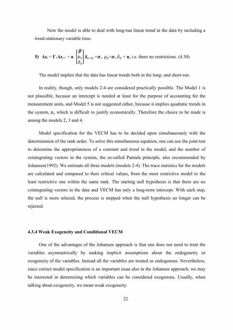
Now the model is able to deal with long-run linear trend in the data by including a

trend-stationary variable time.

5) ∆zt = Γ1∆zt-1 + α }N��~�� R���@ +M� �+M�~ + ut, i.e. there no restrictions. (4.30)

The model implies that the data has linear trends both in the long- and short-run.

In reality, though, only models 2-4 are considered practically possible. The Model 1 is

not plausible, because an intercept is needed at least for the purpose of accounting for the

measurement units, and Model 5 is not suggested either, because it implies quadratic trends in

the system, zt, which is difficult to justify economically. Therefore the choice to be made is

among the models 2, 3 and 4.

Model specification for the VECM has to be decided upon simultaneously with the

determination of the rank order. To solve this simultaneous equation, one can use the joint test

to determine the appropriateness of a constant and trend in the model, and the number of

cointegrating vectors in the system, the so-called Pantula principle, also recommended by

Johansen(1992). We estimate all three models (models 2-4). The trace statistics for the models

are calculated and compared to their critical values, from the most restrictive model to the

least restrictive one within the same rank. The starting null hypothesis is that there are no

cointegrating vectors in the data and VECM has only a long-term intercept. With each step,

the null is more relaxed, the process is stopped when the null hypothesis no longer can be

rejected.

4.3.4 Weak Exogeneity and Conditional VECM

One of the advantages of the Johansen approach is that one does not need to treat the

variables asymmetrically by making implicit assumptions about the endogeneity or

exogeneity of the variables. Instead all the variables are treated as endogenous. Nevertheless,

since correct model specification is an important issue also in the Johansen approach, we may

be interested in determining which variables can be considered exogenous. Usually, when

talking about exogeneity, we mean weak exogeneity.

23

Consider two stochastic variables, yt and xt, and a simple data generating processes for

yt and xt:

�� � ��3� � ����� � �� (4.31)

3� � 23��� � ��� , where |�2 | < 1 and �� ~ (0, ��) (4.32)

The second variable, xt, is said to be strongly exogenous to the first one, yt, if it is

possible to treat xt as fixed in (4.31), i.e. E(3���� � _. This is possible if the two error terms

are not correlated, E(����� � _. The exogenous variable xt is considered weakly exogenous if

it still can be treated as fixed, i.e. E(3���� � _, but equation (4.32) also contains past values

of yt,:

3� � 2�3��� � 2���� � ��� (4.33)

In this case xt and yt both are influenced by own past values and past values of each

other, but the weakly exogenous xt is not correlated with the error term in the equation for yt.

(Harris & Sollis, 2005).

In Johansen (1995) framework testing for weak exogeneity amounts to testing whether

some variable’s speed of adjustment vector, M�W�� � ���� ��������� � � 1�� � �� in the

cointegration system is equal to zero, and it is therefore said that the variable is weakly

exogenous to the system. The system loses no information if the short-run determinants of ∆zit

are not modeled when estimating the parameters [Γ, α, β, Π] of the model, although

Mp��remains in the long-run model.

When having concluded that a particular variable is weakly exogenous, we can proceed

with a conditional, or partial, model:

B��� �=� ��M�NY=��� � � B���@����� �=��� ����� (4.34)

where �P� � �����P is Gaussian Np (0, ��), the variance matrix �� � ���������Y. Harris and Sollis (2005) give two reasons why one should test the variables in an

unrestricted model for weak exogeneity when using the Johansen approach and construct the

conditional model. One potential advantage of a conditional model against the unrestricted

one is that the restricted model might have better stochastic properties if the “problematic”

24

features happen to be concentrated to the variable(s) that is(are) found to be weakly

exogenous to the system. By better stochastic properties is meant that the residuals of the

short-run equations in the conditional model are free from unwanted features.

The second advantage of the conditional model is that it reduces the number of short-

run variables in the VECM, which makes it computationally easier to deal with the short-run

model.

Despite the named advantages Harris and Sollis (2005) do not recommend to assume

weak exogeneity and start with a conditional model, but to start with a general model and later

test for exogeneity. The reasons are that conditioning affects the asymptotic distributions of

the rank test statistics, and that one usually wants to test for exogeneity, not just assume it.

In reality, testing for weak exogeneity is usually done alongside with testing hypotheses

on the cointegration coefficients vector β. That is due to the fact that a given cointegration

vector can indeed be a vector describing a structural relationship between the variables, or it

can be just a linear combination of stationary vectors. The latter is possible because the

Johansen approach shows how many cointegrating vectors β span the cointegration space. But

a linear combination of cointegrating vectors (which are stationary) results in a new stationary

vector, and therefore the cointegrating vectors we obtain may not be unique.

4.3.4.1 Limitations of the Johansen Approach

Despite the numerous advantages the Johansen approach has over the Engle- Granger

approach, the Johansen method suffers from some deficiencies itself. Two of the limitations

have to do with the fact that Johansen approach is based on VAR systems. Because the

variables in a VAR system are treated symmetrically as endogenous, it is not as

straightforward to read the output in the Johansen method and to interpret the results in terms

of exogenous and endogenous variables, as it is in the Engle-Granger approach. The second

disadvantage of the method is due to that all the variables are modeled simultaneously, which

can cause problems if any of the variables are flawed, e.g. the VAR system can be biased. To

mitigate this, one could condition on the problematic variable, instead of having the

25

unrestricted model (see also section 4.3.4, the part on weak exogeneity). And, finally, a

multidimensional VAR system consumes many degrees of freedom. ( Sörensen,1997).

Another weakness of the Johansen method is that it does not always fulfill the

transitivity property. The Johansen test can fail to detect a cointegrating relationship between

two variables, A and B, that are cointegrated with each other through the fact that both A and

B are cointegrated with a third variable, C. Ferré (2004) explains the paradox by the behavior

of the residuals and their variances in the relationship between the variables.

The Johansen method is very sensitive to model specification of the VECM, particularly

when it comes to deterministic components in the model. Including or excluding a linear trend

component can make all the difference between the robust positive results and the unfavorable

ones (Ahking 2002).

4.3.5 Vector Error Correction Granger-Causality Test

When investigating the causal relationships between different time series, two strategies

are identified by Kirchgässner and Wolters (2007). The first one is the bottom up strategy

with the assumption that the time series are generated independently of each other. Granger

(1969) popularized this strategy with causality test and tried to answer whether there are some

specific time series that are related to each other. The other one is the top down strategy under

the assumption that the generating process is not independent; hence it aims to find out

whether some specific time series are generated independently.

4.3.5.1 Bottom Up Approach

Granger (1969) defines the causality between the weakly stationary time series x and y

as follows: x is (simply) Granger causal to y if and only if the application of an optimal linear

prediction function leads to:

σ2 (yt+1 | It ) < σ2 (yt+1 | It-����� ), (4.35)

where It is the information set, includes the two time series X and Y, available at time t.

�����is the set of all current and past value of X. �����={xt, xt-1, …xt-k, …}

26

σ2 (·) is the variance of the corresponding forecast error which indicates with a smaller

forecast error variance, the future value of y could be predicted better within the current and

past values of x available.

a) The direct bivariate Granger procedure

Sargent (1976) derives a simple procedure for testing the causality directly from

Granger definition of causality. Regressing two stationary variables, x and y, using the

following equation:

�� ��� ������ ��� � � 2����� ��� � �� (4.36)

�� ��� ~����� ��� � � ������ ��� � �� (4.37)

Wald test is used to test whether all of the lagged values of X in the Y equation are

simultaneously equal to zero in order to find out whether X Granger-causes Y.

If 0β ≠∑ , X Granger causes Y;

If both 0δ ≠∑ and 0β ≠∑ , then there exists a bidirectional causality between Y and X.

b) Granger Causality in a trivariate Model

The simple Granger procedure could be extended since it is possible that a third variable

would affect the variables under consideration. If the information set It contains the past

information on a third variable Z besides ��� and ��� , the null hypothesis of X does not cause Y

conditional on Z could be tested with a Wald test in a model where Y depends on lagged

values of Y and Z.

4.3.5.2 Top down Approach

When it comes to VAR models, causality is tested on the basis of the pre-testing for unit

roots and cointegration. If the time series are stationary, then a VAR model in levels is

constructed. If the variables are difference stationary, or integrated of order one, I(1), the

VAR is specified in first differences. If the series are cointegrated then vector error correction

(VECM) models are used. Sims et al (1990) show that if the variables are cointegrated of

order 1, Wald tests of Granger non-causality in levels VAR could be used based on the error

27

correction model. Toda and Phillips (1993) further improve this and point out that the Wald

tests are valid asymptotically if there is sufficient cointegration among the variables. As

Granger representation theorem7 suggests, if the variables are cointegrated then there must be

a causal relationship among them running at least in one direction, and therefore a pairwise

Granger causality and VEC Granger-causality test for zero restrictions on the coefficients on

the VAR or VEC model can be employed.

When we know that some, or all, variables in our VAR are cointegrated (from the

reduced rank regression results), we would like to know what the causal relationships between

them are. To obtain the answer we utilize the VEC Granger-Causality Test. One has to

understand from the beginning the actual meaning of the VEC Granger-causality test. The test

does not say that changes in one variable cause changes in another. What Granger-causality

test gives is the correlation between the current value of one variable and past values of the

other variables. That is, if we say that x1t , x2t, …, xnt Granger-cause yt , we mean that past

value(s) of xit (i= 1,2,…,n) are correlated with the current value of yt. Granger-causality can

go in one direction between two variables, both ways, or there is no Granger-causality at all.

(Brooks, 2008)

7 Granger representation theorem: Let xt ∼ I(1) and yt ∼ I(1) then xt and yt are cointegrated if and only if there exist theerror correction model (ECM) such that ∆xt = −γ1zt−1 +lagged(∆xt,∆yt)+δ(L)ε1t ∆yt = −γ2zt−1 +lagged(∆xt,∆yt)+δ(L)ε2t, Where zt = yt − Axt ∼ I(0) δ(L) = 1+δ1L+· · ·+δpLp.is the same in both equations, and |γ1| +|γ2| ≠ 0 (Engle and Granger 1987).

ii

5. Empirical Results and Analysis

We carry out the tests on the nine commodities mentioned in Data part using the

statistical software EViews 7.0 in three stages. Firstly, the unit root tests are applied to

examine whether all the time series are stationary. If it is established that non-stationarity

exist, Johansen test is utilized to check for cointegration relationship(s). On the basis of these

tests, lead-lag relations are assessed at the end.

Our tests follow the steps below:

1. Testing the order of integration of each time series that is in the multivariate model;

2. Setting the appropriate lag length of the VAR model;

3. Formulating the optimal Vector Error Correction model with regards to

deterministic components (trend and intercept) in the long- and short-run part of the

VECM among the five possible models;

4. Testing for the weak exogeneity;

5. Testing for the unique cointegration vectors and joint tests involving restrictions on

α and β;

6. Identifying the lead-lag relationships between the commodities by using VEC

Granger-Causality test.

5.1 Integration: Unit root tests and stationarity test results

Augmented Dickey-Fuller (ADF) (1979) test is conducted on the logged price levels

using the lag structure indicated by Schwarz Information Criterion (SIC), see the table below.

We start our unit root test with the most general model, containing an intercept and a trend:

F�� � �� � �: � ����� � �¡�F���� � �� (5.1)

We test the following null hypothesis

H0: � � _� ; Time series is non stationary

H1: � _�; Time series is stationary.

29

Next we test for the presence of a trend by setting��: � _:

F�� � �� ������ � �¡�F���� � �� (5.2)

And, finally, we test for the presence of a drift, by adding one more restriction, namely

�� � _ :

F�� � ����� � �¡�F���� � � (5.3)

Phillips–Perron (PP) tests and KPSS test (Kwaitkowski et al.1992) are conducted to

double check the results obtained from the ADF test. The PP test has the same null hypothesis

as the ADF test while the KPSS test has the opposite null hypothesis, i.e. that the time series

is stationary. All the three tests give the consistent results presented in Appendix H Table7.

The results indicate that we are unable to reject the null hypothesis for any the nine

commodities at any of the three significance levels commonly used: 1% level, 5% level and

10% level, which means there exists a unit root in each time series. To test whether there are

two unit roots, the same procedure is applied to the first differences (see Appendix I Table 8)

under the same hypotheses. The results are equally conclusive and indicate that the time series

are stationary at first difference. Thus, all the variables are integrated of order one and

stationary upon differencing once, this also supports Brooks (2008)’s statement that the

majority of financial and economic time series contain a single unit root.

5.2 Cointegration: Johansen test results

We have tested the variables for stationarity and the number of unit roots, and have

come to that the ordinary Johansen method, which is designed for variables with at most one

unit root, can be applied. We proceed by formulating the appropriate vector autoregression

model (VAR) (see Appendix J Table 9). The Akaike information criteria indicate that two lags

should be included. Next, applying the Pantula principle we arrive to the conclusion that

Model 2 and rank 2 describe the data best (see equation(4.27)) where zt = [ALUM_ALLOYt,

ALUMINIUMt COPPERt, GOLDt, LEADt, NICKELt, OILt, TINt, ZINCt]

The test for exogeneity reveals that Copper, Nickel and Tin are weakly exogenous

variables in the system, and thus the model can be conditioned upon them.

30

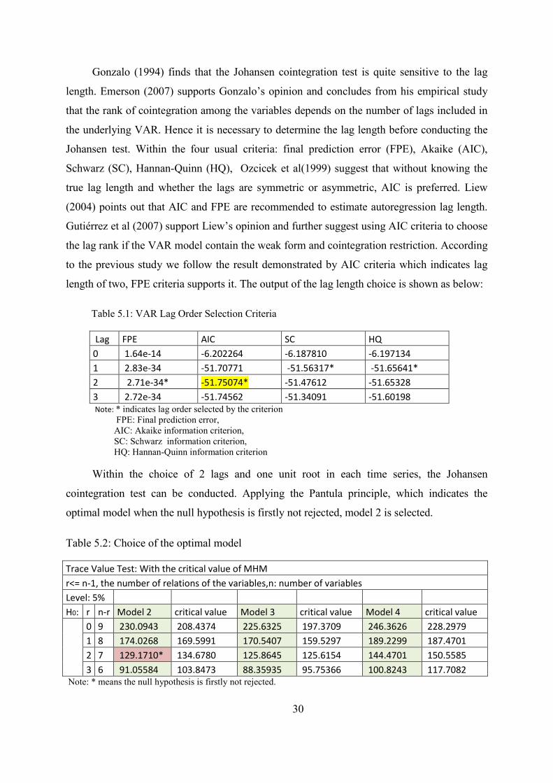
Gonzalo (1994) finds that the Johansen cointegration test is quite sensitive to the lag

length. Emerson (2007) supports Gonzalo’s opinion and concludes from his empirical study

that the rank of cointegration among the variables depends on the number of lags included in

the underlying VAR. Hence it is necessary to determine the lag length before conducting the

Johansen test. Within the four usual criteria: final prediction error (FPE), Akaike (AIC),

Schwarz (SC), Hannan-Quinn (HQ), Ozcicek et al(1999) suggest that without knowing the

true lag length and whether the lags are symmetric or asymmetric, AIC is preferred. Liew

(2004) points out that AIC and FPE are recommended to estimate autoregression lag length.

Gutiérrez et al (2007) support Liew’s opinion and further suggest using AIC criteria to choose

the lag rank if the VAR model contain the weak form and cointegration restriction. According

to the previous study we follow the result demonstrated by AIC criteria which indicates lag

length of two, FPE criteria supports it. The output of the lag length choice is shown as below:

Table 5.1: VAR Lag Order Selection Criteria

Lag FPE AIC SC HQ 0 1.64e-14 -6.202264 -6.187810 -6.197134 1 2.83e-34 -51.70771 -51.56317* -51.65641* 2 2.71e-34* -51.75074* -51.47612 -51.65328 3 2.72e-34 -51.74562 -51.34091 -51.60198 Note: * indicates lag order selected by the criterion

FPE: Final prediction error, AIC: Akaike information criterion, SC: Schwarz information criterion, HQ: Hannan-Quinn information criterion

Within the choice of 2 lags and one unit root in each time series, the Johansen

cointegration test can be conducted. Applying the Pantula principle, which indicates the

optimal model when the null hypothesis is firstly not rejected, model 2 is selected.

Table 5.2: Choice of the optimal model

Trace Value Test: With the critical value of MHM r<= n-1, the number of relations of the variables,n: number of variables Level: 5% H0: r n-r Model 2 critical value Model 3 critical value Model 4 critical value 0 9 230.0943 208.4374 225.6325 197.3709 246.3626 228.2979 1 8 174.0268 169.5991 170.5407 159.5297 189.2299 187.4701 2 7 129.1710* 134.6780 125.8645 125.6154 144.4701 150.5585 3 6 91.05584 103.8473 88.35935 95.75366 100.8243 117.7082 Note: * means the null hypothesis is firstly not rejected.

31

There are two kinds of cointegration tests, maximal eigenvalue test and trace test. Toda

(1994) reports that within small-sample properties, trace test performs better than the other

one when the power is low. Lutkepohl et al (2001) confirm this and conclude a preference of

trace tests from their study as well. Hence we follow the trace test; the result is shown in

Table 5.3 (For the whole table see Appendix K Table 10).

Table 5.3: Unrestricted Cointegration Rank Test (Trace)

Hypothesized Trace 0.05 No. of CE(s) Eigenvalue Statistic Critical Value Prob.** None * 0.014234 230.0943 208.4374 0.0029 At most 1 * 0.011404 174.0268 169.5991 0.0286 At most 2 0.009698 129.1710 134.6780 0.1007 At most 3 0.008065 91.05584 103.8473 0.2579

Note: * denotes rejection of the hypothesis at the 0.05 level **MacKinnon-Haug-Michelis (1999) p-values

The trace test indicates that there exist two cointegrating vectors at the 5% level which

means there are two linear combinations among the variables.

5.3 Tests for the Separate Models

The tests indicate that there are two cointegrating vectors among the nine variables.

However, it is a well-known problem to identify the unique cointegrating vectors, i.e. to

identify the restrictions on β, when there are more than one cointegration equations and there

is no strong theory to backup the restrictions, as in our case (Larsson et al, 2010). To reduce

the number of the cointegrating vectors to one, we test Aluminum and Aluminum Alloy

separately for cointegration and Granger-causality. If they are cointegrated, we exclude

Aluminum Alloy from the original nine-variable group. The reason we exclude Aluminum

Alloy instead of Aluminum is their respective average inventory volume, 67,382.96 against

1,106, 364.35 metric tons (See Table 3.1). Thus, we continue with the remaining eight

variables.

32

5.3.1 Tests Results for Aluminum and Aluminum Alloy

Aluminum and Aluminum Alloy are tested for cointegration by using both the Engle-

Granger univariate method and the Johansen multivariate method.

Firstly, the long run relationship by regressing Aluminum on Aluminum Alloy and a

constant is formulated. Next, we test the residuals for unit root(s) with the ADF test. The

standard ADF critical values in this test can not be used since the unit root test is applied to

residuals but not raw data. Instead, we calculate the critical values as explained by McKinnon

(1996) and check the test-statistic against them. With the implication of the results that the

residuals are stationary, we conclude that the two variables are indeed cointegrated. The

results are double checked by repeating the Engle-Granger test, but with the roles for the two

variables reversed: aluminum alloy is the endogenous variable this time. The output for the

regressions is given in the Appendix M Table 12. The residuals are tested for unit root in the

same way as before and the previous result is confirmed. Finally, the Granger-causality test is

conducted to determine the direction of the relationship and the result indicates that the two

variables share a bi-directional relationship (See Appendix N Table 13). The Johansen method

gives results identical to those obtained with the Engle-Granger method (Appendix Q-R Table

16-17). According to table 3.1, the average inventory volume of Aluminum Alloy is far less

than that of Aluminum, which is 67,382.96 compared to 1,106,364.35. Therefore, Aluminum

Alloy is removed from the group and Johansen method is applied just on the eight-variable

group, i.e. zt = [ ALUMINIUMt, COPPERt, GOLDt, LEADt, NICKELt, OILt, TINt, ZINCt].

5.3.2 Tests Results for the Eight-Variable Group

The tests conducted are the same as before starting with formulating the VAR. The

Akaike Information Criteria suggests two lags (Appendix S, Table 18). Then, the rank and the

model are determined simultaneously using the Pantula principle. Model 2 (see equation 4.27)

is selected and one cointegrating vector is found (See Appendix T, Table 19).

Table 5.4: Unrestricted Cointegrating Coefficients

ALMN Copper Gold Lead Nickel Oil Tin Zinc C -12.35154 4.679840 -3.472042 0.608426 2.937729 -0.222967 -0.913560 0.226387 51.92919

33

Table 5.5: Unrestricted Adjustment Coefficients (alpha)

D(ALMN) D(Copper) D(Gold) D(Lead) D(Nickel) D(Oil) D(Tin) D(Zinc)

0.001093 0.001084 0.000441 0.001506 0.000408 0.001398 0.000776 0.001071

Table 5.4 and 5.5 above display the estimated coefficients of α and β for each variables

individually. However, the individual coefficients do not provide us with useful information,

since they do not say anything about the relationships between the variables. Thus, we need

ratios between individual coefficients which are acquired by normalizing on the coefficient of

a certain variable in the system (Johansen, 1995). After formulating the unrestricted Vector

Error Correction Model, normalized on Aluminum, the results of t-statistics for the

cointegrating vector β are acquired. The results show that cointegrating coefficients for

Aluminum, Copper, Gold and Nickel are significant at 5% level. (See Table 5.6 and Appendix

U Table 20 for the full output).

Table 5.6 Unrestricted Cointegrating Coefficients (Normalized β coefficient on Aluminum to 1)

Almn(-1) Copper(-1) Gold(-1) Lead(-1) Nickel(-1) Oil(-1) Tin(-1) Zinc(-1) C 1.000000 -0.378887 0.281102 -0.049259 -0.237843 0.018052 0.073963 -0.018329 -4.204268

(0.09485) (0.08780) (0.07894) (0.05579) (0.04682) (0.08125) (0.06578) (0.45480)

[-3.99458] [ 3.20159] [-0.62404] [-4.26292] [ 0.38552] [ 0.91031] [-0.27864] [-9.24422] Note: (-1) means difference once, standard errors in ( ) & t-statistics in [ ], Log likelihood: 88088.43

The coefficients of β are interpreted as follows.

ALUMINIUMt = 0.378887COPPERt - 0.281102GOLDt + 0.049259 LEADt + 0.237843 NICKELt -0.018052OILt - 0.073963TINt + 0.018329ZINCt + 4.204268

Copper and Nickel have a positive relationship with Aluminum. 1% increase of Copper

will lead to 0.37% increase of Aluminum in the long term; 1% increase in Nickel will lead to

0.23% increase in Aluminum in the long term; while the coefficient of Gold shows a negative

relationship with Aluminum which indicates 1% increase in Gold will lead to 0.28% decrease

in Aluminum in the long term.

Table 5.7 below displays the speed of adjustment back to the equilibrium represented by

the error correction term. Aluminum has the fastest speed of adjustment while Nickel has the

slowest one. These imply that in the short run, all commodities respond to their last period’s

equilibrium error. Besides, the error correction term of Nickel is not significantly different

from zero which indicates weak exogeneity of the variable.

34

Table 5.7 Speed of adjustment for unrestricted model (Alpha Vector)

D(Almn(-1)) D(Copper(-1)) D(Gold(-1)) D(Lead(-1)) D(Nickel(-1)) D(Oil(-1)) D(Tin(-1)) D(Zinc(-1))

-0.013500 -0.013384 -0.005451 -0.018606 -0.005043 -0.017266 -0.009580 -0.013229

(0.00258) (0.00345) (0.00202) (0.00403) (0.00461) (0.00447) (0.00317) (0.00361)

[-5.24193] [-3.87739] [-2.70396] [-4.61153] [-1.09515] [-3.86042] [-3.02158] [-3.66109] Note: (-1) means difference once, standard errors in ( ) & t-statistics in [ ]

To investigate whether a conditional model would be a better choice, weak exogeneity

of the variables is tested. The results indicate that Nickel and Tin are weakly exogenous (See

Appendix V Table 21). Due to lack of a strong economic theory on which to base β-

restrictions, we only condition the VECM on the speed-of-adjustment coefficients α and the

only restriction on β is the normalization on one β coefficient, which is a restriction but not a

constraint and therefore it does not affect our results.

Table 5.8 below shows a consistent result with the unrestricted model with only a slight

difference. A 1% increase in Copper and Nickel will lead to 0.5% and 0.12% increase,

respectively, in Aluminum. 1% increase in Gold will lead to a 0.41% decrease in Aluminum.

The restricted model displays a much stronger relationship among Aluminum, Copper and

Gold.

Table 5.8 Restricted Cointegrating Coefficients (Normalized β coefficient of Aluminum to 1)

Almn(-1) Copper(-1) Gold(-1) Lead(-1) Nickel(-1) Oil(-1) Tin(-1) Zinc(-1) C 1.000000 -0.504197 0.410922 0.023726 -0.121061 -0.038550 -0.056756 0.008392 -4.389347

(0.08165) (0.07558) (0.06795) (0.04803) (0.04031) (0.06994) (0.05663) (0.39151)

[-6.17504] [ 5.43676] [ 0.34915] [-2.52058] [-0.95636] [-0.81145] [ 0.14820] [-11.2114] Note: (-1) means difference once, standard errors in ( ) & t-statistics in [ ], Log likelihood: 88086.99

Table 5.9 exhibits the speed of adjustment when taking the weakly exogenous variables

into account and it shows that after omitting Nickel and Tin, all other variables are significant

at 5% level.

Table 5.9 Speed of adjustment for unrestricted model (Alpha Vector)

D(Almn(-1)) D(Copper(-1)) D(Gold(-1)) D(Lead(-1)) D(Nickel(-1)) D(Oil(-1)) D(Tin(-1)) D(Zinc(-1)) -0.015005 -0.009304 -0.005781 -0.016617 0.000000 -0.013998 0.000000 -0.013613

(0.00260) (0.00329) (0.00236) (0.00416) (0.00000) (0.00524) (0.00000) (0.00358)

[-5.76092] [-2.82664] [-2.45298] [-3.99135] [ NA] [-2.67189] [ NA] [-3.80358] Note: (-1) means difference once, standard errors in ( ) & t-statistics in [ ]

35

The graph and the output for the restricted VECM are given in the Appendix W Table

22. It can be seen that the model is improved with conditioning on these variables, since now

the fluctuations are concentrated closer around the long-run equilibrium.

Finally, we look at the directions of the cointegrating relationships through the VEC

Granger-causality test in both the unrestricted (Appendix X Table 23) and restricted models

(Appendix Y Table 24). The results are virtually identical for the two models which indicate

that Aluminum is Granger-caused by Copper, but Aluminum itself Granger-causes Gold.

Copper shows bi-directional causality with Gold, whereas Nickel seems to lack causality with

the other three commodities. Additionally, the VEC Granger-causality test indicates that there

exist other causality relations. At 5% significance level all variables, except Lead, are

cointegrated, since there is a causality relationship in at least one direction. Oil is Granger-

caused by Aluminum. Copper Granger-causes Zinc and Tin Granger causes Aluminum. Tin

itself is Granger-caused by Nickel. At 10% significance level all eight variables seem to be

cointegrated. Copper starts to Granger-cause Lead. Both Copper and Oil Granger-cause Tin.

Gold Granger-causes Zinc while Zinc Granger-causes Aluminum. On the block level,

Aluminum, Copper, Gold, Tin and Zinc are Granger-caused by the other seven variables on

both 5% and 10% significance level.

It is an interesting question why the Johansen method and the VEC Granger-causality

test give different results when it comes to the number of cointegrating relationships. We

know that the results in the VEC Granger-causality test are dependent on the way the

variables are ordered in. But the changes are not large enough to explain the discrepancy.

Since the main focus in this paper is the Johansen method, we only use the Granger-causality

test to see the direction in the cointegration relationships suggested by the Johansen method

results. Investigation of the causes for the different results in the two tests should be an

interesting topic for further research. Our guess is that some of our variables are cointegrated

through other (macroeconomic) variables, that are not included in our group, and the Johansen

approach is failing to fulfill the transitivity condition in the cointegrating relationships (see

section Limitations of the Johansen Approach).

36

6. Limitations of the Study and Suggestions for Further Research

Some limitations of this study are identified in the area of Data and Methodology. For

the data part, only daily data with just one time interval, 15 years from 1995 to 2010, is used

due to time and space constraints of this study. The study could have been improved with

additional tests on different time frequencies beside daily data such as weekly, monthly and

/or quarterly. Furthermore, the 15-year time period could also be both extended and

complemented with different sub-samples, e.g. five-year, ten-year, etc. Moreover, the number

of commodities in this paper is limited to nine due partly to the lack of data for some

commodities traded on the LME and the software used. E-Views 7.0 allows at most 10

variables to be tested with the Johansen approach. More variables would probably reveal

more long-term relationships.

The methodology used, with the emphasis on the Johansen approach, potentially limits

the quality of the study. The Johansen method has both own weaknesses (see Section 4.3.4.1)

and shares the common weakness of other linear cointegration methods. Firstly, it is

potentially unable to detect cointegration between variables that are cointegrated through

cointegrating relationship with a common variable. Secondly, it is difficult to test hypothesis

by imposing restrictions on the cointegrating coefficients, i.e. vector β, as well as interpret the

results without a strong economic theory. Also, as a method for linear cointegrating

relationships, the Johansen method can not detect possible non-linear cointegration between

variables. Therefore, we would suggest replicating the study with different linear and non-

linear methods

Consideration should have been taken for the important macroeconomic shocks, e.g. the

latest global financial crisis, when designing the study. During financial crises it is common

that both volatility of assets and their correlations with other assets increase, probably

affecting their cointegration patterns as well.

37

7. Conclusion

The purpose of this study is to investigate the potential long-term relationships among

base metals as well as between base metals, Crude oil and Gold. The results obtained from the

tests indicate that there exist several cointegrating relationships among the base metals. Some

of the base metals seem to have long run relationship with both Crude oil and some with

Gold. However, the results for Gold and Crude oil do not show any cointegration with each

other.

More specifically, Aluminum, Copper, Gold and Nickel are cointegrated according to

the Johansen Approach. The VEC Engle-Granger Causality test indicates more cointegrating

relationships exist within the eight-variable group. At the 10 % significance level all eight

variables are cointegrated with at least one of the remaining seven variables. Therefore,

diversification possibilities for the long-term perspective are generally poor among the base

metals, between the base metals and Gold as well as between base metals and Crude Oil. But

since no cointegration is detected between Gold and Crude Oil, diversification benefits exist

between the two commodities.

According to the results, price developments of Aluminum and especially Copper

should be given more attention. The two metals Granger-cause several other commodities in

the group. Therefore, Aluminum and Copper have lead-lag relationships with the variables

they Granger-cause.

38

8. References

Ahking, F. W., 2002. Model Mis-specification and Johansen's Cointegration Analysis: an Application to the U.S. Money Demand. Working Paper. [Online] Available at (Only the Abstract): http://papers.ssrn.com/sol3/papers.cfm?abstract_id=306841. [Accessed 23 April 2010]. Alexander, C., 2001, Market Models: A guide to Financial Data Analysis, Chichester (UK): John Wiley & Sons Ltd. Asche, F. and Guttormsen, A.G., 2002. Lead Lag Relationships between Futures and Spot Prices. Institute for research in economics and business administration. [Online]. Available at: http://bora.nhh.no/bitstream/2330/898/1/A02_02.pdf . [Accessed 1 April 2010]. Baffes, J., 2007. Oil Spills on other Commodities. Resources Policy, 32(3), pp.126-34 Brooks, C., 2008. Introductory Econometrics for Finance. 8thed. Cambridge: Cambridge University Press. Cashin, P., McDormott, C. and Scott, A., 1999. The Myth of Co-moving Commodity Prices. International Monetary Fund. [Online] Working Paper No.99/169 Available at: http://www.imf.org/external/pubs/cat/longres.cfm?sk=3364.0S [Accessed 25th April 2010] Ciner, C., 2001. On the Long Run Relationship between Gold and Silver Prices A Note. Global Finance Journal, 12(2), pp.299-303. Engle, R.F., and Granger, C.W.J., 1987. Cointegration and Error Correction: Representation, Estimation, and Testing. Econometrica, 55(2), 251-77 Escribano, A.., and Granger, C.W.J., 1998. Investigating the Relationship between Gold and Silver Prices. Journal of Forecasting, 17 (2), pp. 81–107. Ferré, M., 2004. The Johansen Test and the Transitivity Property. Working Paper. [Online] Available at: http://papers.ssrn.com/sol3/papers.cfm?abstract_id=870226&download=yes [Accessed 23 April 2010]. Flood, C., 2010. Gold in Retreat with Base Metals and Oil. Financia Times.[Online] Feb.5,2010. Available at: http://www.ft.com/cms/s/0/a771fbe6-124d-11df-8d73-00144feab49a.html. [Accessed 20th April 2010]. Garbade, K. D., and Silber, W. L., 1983. Price Movement and Price Discovery in Futures and Cash Markets. Review of Economics and Statistics, 65, pp.289–97

39

Goldipedia. 2010. Uses of Gold.[Online]. Available at: http://www.goldipedia.gold.org/uses_of_gold/ [Accessed 19 April 2010]. Gonzalo, J., 1994. A Comparison of Five Alternative Methods of Estimating Long Run Equilibrium Relationships, Journal of Econometrics, 60, pp.203–33. Gutiérrez, C.E.C, Souza, R.C. and Guillén, O.T.C., 2007. Selection of Optimal Lag Length in Cointegrated VAR Models with Weak Form of Common Cyclical Features. Working Paper No. 139. [Online] Available at: http://www.bcb.gov.br/pec/wps/ingl/wps139.pdf [Accessed 14 May 2010] Harris, R.& Sollis, R., 2003, Applied Time Series Modelling and Forecasting, Chichester: John Wiley and Sons. Harvey, J., 2007. Metals - Gold Dips as Dollar Rallies, Oil, Metals Ease. London South East, [Online]. Jul.25, 2007. Available at : http://www.lse.co.uk/FinanceNews.asp?ArticleCode=v2hftahdi039ybi&ArticleHeadline=Metals__Gold_dips_as_dollar_rallies_oil_metals_ease. [Accessed 20 April 2010] Harvard System of Referencing Guide,. [online] July, 2008. Available at: http://libweb.anglia.ac.uk/referencing/harvard.htm [Accessed 20 April 2010] Karl, L., and Nilsson B., 2010. Discussion on Interpreting the Johansen Test Results. [Email] (Personal communication, 18 May 2010) Kirchgässner. G. and Wolters. J, 2007, Introduction to Modern Time Series Analysis, Berlin: Springer-Verlag Johansen, S., 1992. Determination of Cointegration Rank in the Presence of a Linear Trend, Oxford Bulletin of Economics and Statistics, 54(3), pp.383-97 Johansen, S., 1995. Likelihood-Based Inference in Cointegrated Vector Autoregressive Models, USA: Oxford University Press. Johansen, S., Mosconi,R., and Nielsen, B., 2000. Cointegration Analysis in the Presence of Structural Breaks in the Deterministic Trend. Econometrics Journal, 3(2), pp. 216-49

40

Lee, H.S. and Siklos, P.L., 1997. The Role of Seasonality in Economic Time Series -Reinterpreting Money-Output Causality in U.S. Data. International Journal of Forecasting, 13 (3), pp.381-391 Liew, V., 2004. Which Lag Length Selection Criteria Should We Employ? Economics Bulletin, 3(33), pp.1-9 Lüutkepohl, H., Saikkonen,P. and Trenkler C.,2001. Maximum Eigenvalue versus Trace Tests for the Cointegrating Rank of a VAR Process. The Econometrics Journal. 4(2).pp 287-310 Ozcicek, O. and Mcmillin, W., 1999. Lag Length Selection in Vector Autoregressive Models: Symmetric and Asymmetric Lags. Applied Economics, 31(4), pp 517-24 Pantula, S.G., 1989. Testing for Unit Roots in Time Series Data. Econometric Theory, 5(2), pp.256-71 Quantitative Micro Software, LLC. EViews 7.0 User Guide I. Irvine, California, U.S.A.. 29 November 2009. Quantitative Micro Software, LLC. EViews 7.0 User Guide II. Irvine, California, U.S.A.. 29 November 2009. Sari, R., Hammoudeh, S. and Soytas, U., 2010. Dynamics of Oil Price, Precious Metal Prices, and Exchange Rate. Energy Economics, 32(2), pp.351-62 Sargent, T., 1976. A Classical Macroeconomic Model for the United States, Journal of Political Economy, 84(2), pp. 207-37. Silvapulle, P. and Moosa, I. A.., 1999. The Relationship between Spot and Futures Prices: Evidence from the Crude Oil Market. Journal of Futures Markets, 19(2), pp.175-93 Sims, C.A., Stock, J.H., and Watson, M.W., 1990. Inference in linear time series models with some unit roots, Econometrica, 58(1), pp.113–44 Subramanian, U., 2009. Cointegration of Stock Markets in East Asia in the Boom and Early Crisis Period. European Journal of Economics, Finance and Administrative Sciences, [Online] Available at: http://papers.ssrn.com/sol3/papers.cfm?abstract_id=1363914. [Accessed 22 April 2010] Sörensen, B.E., 2005. Cointegration. S.l. Department of Economics, University of Houston [Online] Available at: www.uh.edu/~bsorense/coint.pdf [Accessed 10 April 2010] Toda, H.Y. and Phillips, P.C.B., 1993. Vector Autoregressions and Causality. Econometrica 61(6), pp.1367-93

41

Watkins, C. and McAleer, M., 2002. Cointegration Analysis of Metals Futures. Mathematics and Computers in Simulation, 59(1-3), pp.207-21

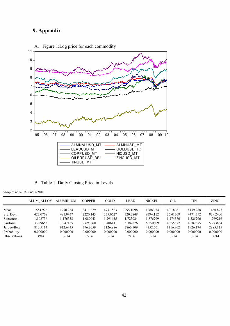
42

9. Appendix

A. Figure 1:Log price for each commodity

B. Table 1: Daily Closing Price in Levels

Sample: 4/07/1995 4/07/2010 ALUM_ALLOY ALUMINIUM COPPER GOLD LEAD NICKEL OIL TIN ZINC Mean 1554.926 1770.764 3411.279 473.1523 995.1098 12883.54 40.18061 8139.268 1460.873

Std. Dev. 423.0768 481.0437 2220.145 235.0627 720.3848 9394.112 26.41368 4471.752 829.2400 Skewness 1.108736 1.176338 1.080043 1.291635 1.723024 1.876299 1.274576 1.525296 1.769216 Kurtosis 3.229653 3.247165 2.693060 3.486411 5.387826 6.550609 4.255872 4.582675 5.273884 Jarque-Bera 810.5114 912.6435 776.3059 1126.886 2866.509 4352.501 1316.962 1926.174 2885.115 Probability 0.000000 0.000000 0.000000 0.000000 0.000000 0.000000 0.000000 0.000000 0.000000 Observations 3914 3914 3914 3914 3914 3914 3914 3914 3914

2

3

4

5

6

7

8

9

10

11

95 96 97 98 99 00 01 02 03 04 05 06 07 08 09 10

ALMNALUSD_MT ALMNUSD_MTLEADUSD_MT GOLDUSD_TOCOPPUSD_MT NICUSD_MTOILBREUSD_BBL ZINCUSD_MTTINUSD_MT

43

C. Table 2: Correlation for daily closing price in levels

ALUM_ALLOY ALUMINIUM COPPER GOLD LEAD NICKEL OIL TIN ZINC ALUM_ALLOY 1.000000

ALUMINIUM 0.967030 1.000000 COPPER 0.913955 0.921467 1.000000 GOLD 0.654331 0.647983 0.845293 1.000000 LEAD 0.768715 0.779582 0.893909 0.836397 1.000000

NICKEL 0.813704 0.867530 0.853857 0.624414 0.788745 1.000000 OIL 0.848394 0.846142 0.909142 0.829395 0.835453 0.740933 1.000000 TIN 0.752799 0.764931 0.875105 0.898253 0.891815 0.703019 0.898333 1.000000

ZINC 0.814823 0.865026 0.861629 0.592985 0.731463 0.885737 0.667578 0.606128 1.000000

D. Table 3: Daily Closing Price in Natural Log

Sample: 4/07/1995 4/07/2010 ALUM_ALLOY ALUMINIUM COPPER GOLD LEAD NICKEL OIL TIN ZINC Mean 7.316428 7.446967 7.951996 6.058551 6.707635 9.263872 3.499841 8.886142 7.169508

Std. Dev. 0.248827 0.245701 0.582752 0.428024 0.585732 0.600383 0.614284 0.460654 0.449870 Skewness 0.743565 0.855032 0.603959 0.816418 0.841343 0.648340 0.286852 0.835877 1.096800 Kurtosis 2.545911 2.631861 1.953429 2.405678 2.585889 2.651839 2.092670 2.671587 3.207872 Jarque-Bera 394.2956 499.0095 416.5762 492.4087 489.7258 293.9729 187.9347 473.3682 791.7848 Probability 0.000000 0.000000 0.000000 0.000000 0.000000 0.000000 0.000000 0.000000 0.000000 Observations 3914 3914 3914 3914 3914 3914 3914 3914 3914

E. Table 4: Correlation for daily closing price in natural log

ALUM_ALLOY ALUMINIUM COPPER GOLD LEAD NICKEL OIL TIN ZINC ALUM_ALLOY 1.000000

ALUMINIUM 0.960145 1.000000 COPPER 0.899511 0.916678 1.000000 GOLD 0.718079 0.714366 0.904258 1.000000 LEAD 0.804495 0.823033 0.941446 0.918264 1.000000

NICKEL 0.864699 0.889229 0.901524 0.782077 0.855653 1.000000 OIL 0.791973 0.809869 0.864597 0.830584 0.829080 0.879391 1.000000 TIN 0.753359 0.781864 0.903608 0.916327 0.939776 0.803158 0.811807 1.000000

ZINC 0.833540 0.884541 0.885411 0.710364 0.820989 0.840393 0.716071 0.744350 1.000000

44

F. Table 5: Daily Closing price in log return

Date: 04/28/10 Time: 22:30

Sample: 4/10/1995 4/07/2010 ALUM_ALLOY ALUMINUM COPPER GOLD LEAD NICKEL OIL TIN ZINC Mean 4.86E-05 5.94E-05 0.000252 0.000273 0.000338 0.000301 0.000390 0.000292 0.000211

Median 0.000000 0.000000 0.000000 0.000000 0.000000 0.000000 0.000266 0.000000 0.000000 Maximum 0.117145 0.060679 0.117259 0.073820 0.130072 0.133096 0.188557 0.153854 0.096101 Minimum -0.126752 -0.082551 -0.104755 -0.071434 -0.131992 -0.183586 -0.158605 -0.114532 -0.126185 Std. Dev. 0.011668 0.013115 0.017560 0.010258 0.020517 0.023331 0.022692 0.016104 0.018357 Skewness -0.103320 -0.247658 -0.171499 -0.039291 -0.155839 -0.081408 -0.087630 -0.144441 -0.306891 Kurtosis 14.69917 5.743632 7.838661 9.756245 6.933179 7.098094 6.982970 11.85065 7.325075 Jarque-Bera 22322.55 1267.299 3836.417 7443.345 2538.076 2742.505 2591.509 12785.32 3111.325 Probability 0.000000 0.000000 0.000000 0.000000 0.000000 0.000000 0.000000 0.000000 0.000000 Sum 0.190313 0.232398 0.986909 1.067205 1.323794 1.176228 1.527833 1.142301 0.824006 Sum Sq. Dev. 0.532591 0.672906 1.206226 0.411680 1.646824 2.129416 2.014330 1.014553 1.318244 Observations 3913 3913 3913 3913 3913 3913 3913 3913 3913

G. Table 6: Correlation for daily closing price in log return

ALUM_ALLOY ALUMINUM COPPER GOLD LEAD NICKEL OIL TIN ZINC ALUM_ALLOY 1.000000

ALUMINUM 0.694661 1.000000 COPPER 0.528346 0.658183 1.000000

GOLD 0.194963 0.232568 0.257800 1.000000 LEAD 0.383624 0.484833 0.542257 0.199266 1.000000

NICKEL 0.363609 0.484731 0.548896 0.169393 0.446381 1.000000 OIL 0.168841 0.171165 0.216860 0.180650 0.184907 0.176690 1.000000 TIN 0.332164 0.398089 0.449068 0.185491 0.393566 0.400016 0.171412 1.000000

ZINC 0.452923 0.593261 0.650764 0.235618 0.588677 0.513227 0.193039 0.410327 1.000000

45

H. Table 7: ADF, PP, KPSS test for I(1)

ADF TEST PP TEST KPSS TEST

H0: time series is non stationary H0: time series is non stationary H0: time series is stationary

T&C T None T&C T None T&C T

AlmnUSD/MT -2,385 -1,448 0,235 -2,346 -1,403 0,245 0,705 3,616

AlmnAlUSD/MT -2,273 -1,071 0,258 -2,538 -1,399 0,185 0,692 3,559

CoppUSD/MT -1,892 -0,114 0,888 -1,887 -0,109 0,892 1,316 4,998

LeadUSD/MT -1,714 -0,464 0,987 -1,664 -0,402 1,033 1,390 5,057

NicUSD/MT -2,034 -0,857 0,749 -2,019 -0,841 0,753 0,642 5,229

TinUSD/MT -1,594 -0,208 1,122 -1,576 -0,185 1,137 1,433 4,874

ZincUSD/MT -1,605 -0,944 0,657 -1,531 -0,864 0,705 0,810 3,350

OilBREUSD/BBL -2,694 -0,829 0,917 -2,686 -0,827 0,918 0,494 6,593

GoldUSD/TO -1,544 1,001 1,729 -1,551 0,992 1,723 1,816 5,756

1% level -3,960 -3,432 -2,566 -3,960 -3,432 -2,566 0,216 0,739

5% level -3,411 -2,862 -1,941 -3,411 -2,862 -1,941 0,146 0,463

10% level -3,127 -2,567 -1,617 -3,127 -2,567 -1,617 0,119 0,347

I. Table 8: ADF, PP, KPSS test for I(2)

ADF TEST PP TEST KPSS TEST

H0: time series is non stationary H0: time series is non stationary H0: time series is stationary

T&C T None T&C T None T&C T

AlmnUSD/MT -64,254 -64,251 -64,258 -64,263 -64,258 -64,265 0,065 0,130

AlmnAlUSD/MT -66,045 -66,024 -66,031 -66,384 -66,391 -66,398 0,072 0,186

CoppUSD/MT -65,412 -65,370 -65,364 -65,347 -65,306 -65,301 0,094 0,394

LeadUSD/MT -59,762 -59,756 -59,748 -59,744 -59,733 -59,720 0,063 0,190

NicUSD/MT -61,892 -61,894 -61,892 -61,889 -61,891 -61,889 0,074 0,113

TinUSD/MT -61,173 -61,157 -61,145 -61,187 -61,156 -61,143 0,050 0,233

ZincUSD/MT -64,372 -64,374 -64,373 -64,433 -64,434 -64,433 0,100 0,152

OilBREUSD/BBL -62,290 -62,295 -62,284 -62,289 -62,294 -62,284 0,041 0,062

GoldUSD/TO -62,160 -62,077 -62,041 -62,168 -62,077 -62,045 0,024 0,653

1% level -3,960 -3,432 -2,566 -3,960 -3,432 -2,566 0,216 0,739

5% level -3,411 -2,862 -1,941 -3,411 -2,862 -1,941 0,146 0,463

10% level -3,127 -2,567 -1,617 -3,127 -2,567 -1,617 0,119 0,347

46

J. Table 9: Vector Autoregression Estimates

Sample (adjusted): 4/11/19954/07/2010

Included observations: 3912 after adjustments ALMNAL ALMN LEAD GOLD COPPER NICKEL OILBRE ZINC TIN

AlmnAlloy(-1) 0,8239 -0,0737 -0,0519 -0,0196 -0,0620 -0,0411 0,0149 -0,0519 -0,0914

Standard errors -0,0223 -0,0252 -0,0395 -0,0198 -0,0338 -0,0450 -0,0438 -0,0354 -0,0310

t-statistics [ 37,0147] [-2,92412] [-1,31400] [-0,99171] [-1,83523] [-0,91210] [ 0,33985] [-1,46740] [-2,94956]

AlmnAlloy(-2) 0,1754 0,0831 0,0464 0,0189 0,0715 0,0511 -0,0109 0,0548 0,0956

Standard errors -0,0223 -0,0252 -0,0395 -0,0198 -0,0338 -0,0451 -0,0439 -0,0354 -0,0310

t-statistics [ 7,87877] [ 3,29445] [ 1,17492] [ 0,95871] [ 2,11407] [ 1,13478] [-0,24929] [ 1,54705] [ 3,08205]

Almn(-1) 0,1951 1,0448 -0,0030 0,0140 -0,0008 -0,0238 0,0288 0,0450 0,0122

Standard errors -0,0232 -0,0263 -0,0412 -0,0206 -0,0352 -0,0469 -0,0457 -0,0369 -0,0323

t-statistics [ 8,41517] [ 39,7786] [-0,07173] [ 0,67855] [-0,02407] [-0,50803] [ 0,63167] [ 1,22039] [ 0,37863]

Almn(-2) -0,2044 -0,0703 -0,0079 -0,0193 -0,0172 0,0104 -0,0432 -0,0617 -0,0172

Standard errors -0,0232 -0,0263 -0,0411 -0,0206 -0,0352 -0,0469 -0,0456 -0,0368 -0,0323

t-statistics [-8,82389] [-2,67786] [-0,19319] [-0,94044] [-0,48765] [ 0,22162] [-0,94689] [-1,67598] [-0,53284]

LEAD(-1) -0,0024 -0,0075 1,0801 0,0165 0,0083 -0,0319 0,0352 0,0142 -0,0047

Standard errors -0,0118 -0,0134 -0,0209 -0,0105 -0,0179 -0,0239 -0,0232 -0,0187 -0,0164

t-statistics [-0,20634] [-0,56446] [ 51,6342] [ 1,57789] [ 0,46299] [-1,33732] [ 1,51822] [ 0,75811] [-0,28421]

LEAD(-2) 0,0060 0,0081 -0,0857 -0,0145 -0,0077 0,0291 -0,0326 -0,0157 0,0086

Standard errors -0,0118 -0,0134 -0,0209 -0,0105 -0,0179 -0,0239 -0,0232 -0,0188 -0,0164

t-statistics [ 0,50932] [ 0,60854] [-4,09711] [-1,38404] [-0,42913] [ 1,22059] [-1,40554] [-0,83566] [ 0,52449]

GOLD(-1) -0,0065 -0,0097 -0,0343 0,9759 -0,0944 0,0039 -0,0233 -0,0765 -0,0239

Standard errors -0,0189 -0,0214 -0,0335 -0,0168 -0,0287 -0,0382 -0,0372 -0,0300 -0,0263

t-statistics [-0,34571] [-0,45181] [-1,02198] [ 58,2141] [-3,29280] [ 0,10138] [-0,62691] [-2,54740] [-0,91027]

GOLD(-2) 0,0060 0,0056 0,0365 0,0212 0,0977 0,0047 0,0215 0,0766 0,0283

Standard errors -0,0189 -0,0214 -0,0336 -0,0168 -0,0287 -0,0383 -0,0372 -0,0301 -0,0263

t-statistics [ 0,31525] [ 0,25965] [ 1,08763] [ 1,26106] [ 3,40348] [ 0,12160] [ 0,57849] [ 2,54998] [ 1,07443]

COPPER(-1) -0,0136 -0,0021 -0,0316 0,0447 0,9993 -0,0469 0,0208 -0,0265 -0,0310

Standard errors -0,0164 -0,0186 -0,0292 -0,0146 -0,0250 -0,0333 -0,0324 -0,0261 -0,0229

t-statistics [-0,82536] [-0,11140] [-1,08452] [ 3,06601] [ 40,0370] [-1,40888] [ 0,64397] [-1,01234] [-1,35492]

COPPER(-2) 0,0143 0,0067 0,0396 -0,0426 -0,0025 0,0447 -0,0200 0,0360 0,0284

Standard errors -0,0164 -0,0186 -0,0292 -0,0146 -0,0250 -0,0333 -0,0324 -0,0261 -0,0229

t-statistics [ 0,86796] [ 0,36201] [ 1,35584] [-2,92038] [-0,09916] [ 1,34337] [-0,61748] [ 1,37585] [ 1,24195]

NICKEL(-1) 0,0030 0,0105 -0,0006 0,0000 0,0012 1,0406 0,0224 -0,0106 0,0524

Standard errors -0,0100 -0,0114 -0,0178 -0,0089 -0,0152 -0,0203 -0,0198 -0,0160 -0,0140

t-statistics [ 0,30291] [ 0,92744] [-0,03544] [-0,00145] [ 0,07795] [ 51,2696] [ 1,13511] [-0,66719] [ 3,75329]

NICKEL(-2) -0,0022 -0,0093 0,0069 0,0003 0,0023 -0,0406 -0,0163 0,0125 -0,0498

Standard errors -0,0100 -0,0114 -0,0178 -0,0089 -0,0153 -0,0203 -0,0198 -0,0160 -0,0140

t-statistics [-0,21417] [-0,81874] [ 0,38629] [ 0,03243] [ 0,15099] [-1,99780] [-0,82677] [ 0,78147] [-3,56450]

OILBRE(-1) -0,0009 0,0041 -0,0042 0,0054 -0,0012 0,0267 0,9923 0,0063 0,0007

Standard errors -0,0085 -0,0096 -0,0150 -0,0075 -0,0128 -0,0171 -0,0167 -0,0134 -0,0118

47

t-statistics [-0,10700] [ 0,43063] [-0,28041] [ 0,71755] [-0,09725] [ 1,56305] [ 59,6047] [ 0,46577] [ 0,05700]

OILBRE(-2) 0,0023 -0,0023 0,0021 -0,0042 0,0023 -0,0264 0,0038 -0,0062 -0,0018

Standard errors -0,0085 -0,0096 -0,0150 -0,0075 -0,0128 -0,0171 -0,0166 -0,0134 -0,0118

t-statistics [ 0,27094] [-0,23975] [ 0,14016] [-0,55397] [ 0,17914] [-1,54614] [ 0,22856] [-0,45933] [-0,15118]

ZINC(-1) -0,0240 -0,0378 -0,0345 0,0058 -0,0303 0,0167 -0,0477 0,9911 0,0050

Standard errors -0,0149 -0,0169 -0,0264 -0,0132 -0,0226 -0,0301 -0,0293 -0,0237 -0,0207

t-statistics [-1,61192] [-2,24489] [-1,30696] [ 0,43610] [-1,34240] [ 0,55465] [-1,62690] [ 41,8891] [ 0,23963]

ZINC(-2) 0,0257 0,0406 0,0350 -0,0057 0,0330 -0,0118 0,0480 0,0077 -0,0037

Standard errors -0,0149 -0,0169 -0,0264 -0,0132 -0,0226 -0,0301 -0,0293 -0,0236 -0,0207

t-statistics [ 1,73085] [ 2,40795] [ 1,32553] [-0,43338] [ 1,46196] [-0,39098] [ 1,63777] [ 0,32448] [-0,17916]

TIN(-1) -0,0234 -0,0138 0,0198 -0,0107 -0,0006 -0,0076 -0,0191 -0,0248 1,0197

Standard errors -0,0134 -0,0152 -0,0238 -0,0119 -0,0204 -0,0271 -0,0264 -0,0213 -0,0187

t-statistics [-1,74294] [-0,90983] [ 0,83202] [-0,89734] [-0,02865] [-0,28182] [-0,72155] [-1,16245] [ 54,5947]

TIN(-2) 0,0191 0,0126 -0,0223 0,0095 -0,0026 0,0025 0,0186 0,0195 -0,0273

Standard errors -0,0134 -0,0152 -0,0238 -0,0119 -0,0204 -0,0271 -0,0264 -0,0213 -0,0187

t-statistics [ 1,42085] [ 0,82890] [-0,93738] [ 0,79823] [-0,12888] [ 0,09346] [ 0,70349] [ 0,91243] [-1,46218]

C 0,0612 0,0787 0,0514 0,0358 0,0396 0,0197 0,0246 0,0767 0,0131

Standard errors -0,0143 -0,0162 -0,0254 -0,0127 -0,0217 -0,0289 -0,0281 -0,0227 -0,0199

t-statistics [ 4,28607] [ 4,86420] [ 2,02758] [ 2,82032] [ 1,82543] [ 0,68131] [ 0,87249] [ 3,37391] [ 0,65856]

R-squared 0,9979 0,9972 0,9988 0,9994 0,9991 0,9985 0,9986 0,9984 0,9988

Adj, R-squared 0,9979 0,9972 0,9988 0,9994 0,9991 0,9985 0,9986 0,9983 0,9988

Sum sq, resids 0,5151 0,6612 1,6226 0,4059 1,1879 2,1089 1,9978 1,3021 0,9991

S,E, equation 0,0115 0,0130 0,0204 0,0102 0,0175 0,0233 0,0227 0,0183 0,0160

F-statistic 101477,80 77052,32 178702,20 381763,40 241733,70 144412,50 159559,50 131311,60 179519,70

Log likelihood 11926,26 11438,06 9682,04 12392,43 10292,04 9169,25 9275,14 10112,48 10630,62

Akaike AIC -6,0876 -5,8380 -4,9402 -6,3259 -5,2521 -4,6780 -4,7322 -5,1603 -5,4252

Schwarz SC -6,0571 -5,8075 -4,9097 -6,2954 -5,2216 -4,6476 -4,7017 -5,1298 -5,3947

Mean dependent 7,3163 7,4469 6,7078 6,0586 7,9520 9,2640 3,5001 7,1696 8,8863

S,D, dependent 0,2489 0,2458 0,5858 0,4281 0,5829 0,6005 0,6143 0,4500 0,4607 Determinant resid covariance (dof adj,) 2,57E-34 Determinant resid covariance 2,46E-34 Log likelihood 101416,1 Akaike information criterion -51,76128 Schwarz criterion -51,48712

48

K. Table 10: Choice of the optimal model Trace Value Test: With the critical value of MHM r<= n-1, the number of relations of the variables,n: number of variables Level: 5%

H0: r n-r Model 2 critical value Model 3 critical value Model 4 critical value 0 9 230.0943 208.4374 225.6325 197.3709 246.3626 228.2979 1 8 174.0268 169.5991 170.5407 159.5297 189.2299 187.4701 2 7 129.1710* 134.6780 125.8645 125.6154 144.4701 150.5585 3 6 91.05584 103.8473 88.35935 95.75366 100.8243 117.7082 4 5 59.38492 76.97277 56.69000 69.81889 69.11097 88.80380 5 4 31.82397 54.07904 29.14251 47.85613 41.09981 63.87610 6 3 16.81814 35.19275 14.14743 29.79707 22.88500 42.91525 7 2 7.694576 20.26184 5.393028 15.49471 13.09607 25.87211 8 1 2.214778 9.164546 0.055022 3.841466 5.066655 12.51798

Note: * means the null hypothesis is firstly not rejected. L. Table 11: MacKinnon Critical Value n = 2(Total number of time series) Dep.variable: Critical value = φ∞ + φ1/T + φ2/T^2 (T: Number of observations) Aluminum Alum Alloy

Model Significance (%) φ∞ φ1 φ2 Crit.Values ADF t-stat ADF t-stat constant 1 -3,900 -10,534 -30,030 -3,903 -3,973 5 -3,338 -5,967 -8,980 -3,339 -3.866399 10 -3,046 -4,069 -5,730 -3,047 constant and trend 1 -4,327 -15,531 -34,030 -4,331 5 -3,781 -9,421 -15,060 -3,783 -3,952 -3.896110 10 -3,496 -7,203 -4,010 -3,498

(source: MacKinnon 2010 & Hjertstrand P.2010)

49

M. Table 12: VAR Lag Order Selection Criteria for Aluminum and Aluminum Alloy

VAR Lag Order Selection Criteria

Endogenous variables: ALMNALUSD_MT ALMNUSD_MT

Exogenous variables: C

Sample: 4/07/1995 4/07/2010

Included observations: 3864 Lag LogL LR FPE AIC SC HQ

0 4735.755 NA 0.000296 -2.450184 -2.446944 -2.449033

1 24257.14 39012.45 1.21e-08 -12.55235 -12.54263 -12.54890

2 24316.76 119.0944 1.18e-08 -12.58114 -12.56494* -12.57539*

3 24323.07 12.58472 1.18e-08 -12.58233 -12.55965 -12.57428

4 24327.73 9.309725 1.18e-08 -12.58268 -12.55352 -12.57232

5 24328.87 2.278875 1.18e-08 -12.58120 -12.54556 -12.56854

6 24337.37 16.94172 1.18e-08 -12.58353 -12.54141 -12.56857

7 24339.53 4.303302 1.18e-08 -12.58257 -12.53398 -12.56532

8 24342.31 5.527217 1.18e-08 -12.58194 -12.52686 -12.56238

9 24346.72 8.767334 1.18e-08 -12.58215 -12.52059 -12.56029

10 24351.51 9.536597 1.18e-08 -12.58256 -12.51452 -12.55840

11 24356.63 10.17911 1.18e-08 -12.58314 -12.50862 -12.55668

12 24359.62 5.947562 1.18e-08 -12.58262 -12.50162 -12.55386

13 24365.10 10.87278 1.18e-08 -12.58338 -12.49591 -12.55232

14 24367.28 4.330787 1.18e-08 -12.58244 -12.48849 -12.54908

15 24374.06 13.45794 1.17e-08* -12.58388* -12.48345 -12.54822

16 24375.61 3.061151 1.18e-08 -12.58261 -12.47570 -12.54465

N. Table 13: Pairwise Granger Causality Test for Aluminum and Aluminum Alloy Pairwise Granger Causality Tests

Sample: 4/07/1995 4/07/2010

Lags: 2 Obs: 3912 Null Hypothesis: F-Statistic Prob. Aluminum Alloy does not Granger Cause Aluminum 10.4600 3.E-05 Aluminum does not Granger Cause Aluminum Alloy 33.4454 4.E-15

O. Table 14: Identify the optimal model for Aluminum and Aluminum Alloy Trace Test: With the critical value of MHM r<= n-1, the number of relations of the variables,n: number of variables Level: 5% H0: r n-r Model 2 critical value Model 3 critical value Model 4 critical value 0 9 23.09927 20.26184 22.98777 15.49471 28.91358 25.87211 1 8 2.729943* 9.164546 2.644508 3.841466 8.548827 12.51798

50

P. Table 15: Restrictions on Alpha Restrictions on Alpha prob. a(1,1)=0 0.502986 a(2,1)=0 0.000680

Q. Table 16: Cointegration test without restriction Vector Error Correction Estimates

Sample (adjusted): 5/01/1995 4/07/2010

Included observations: 3898 after adjustments

Standard errors in ( ) & t-statistics in [ ]

Cointegrating Eq: CointEq1

ALMNALUSD_MT(-1) 1.000000

ALMNUSD_MT(-1) -0.996424

(0.06127)

[-16.2620]

C 0.106721

(0.45650)

[ 0.23378]

Error Correction: D(ALMNALUSD_MT) D(ALMNUSD_MT)

CointEq1 -0.000469 0.009608

(0.00273) (0.00310)

[-0.17184] [ 3.09813]

-.3

-.2

-.1

.0

.1

.2

.3

95 96 97 98 99 00 01 02 03 04 05 06 07 08 09 10

Cointegrating relation 1

51

R. Table 17: Cointegration test with restriction a(1,1)=0 Vector Error Correction Estimates Date: 05/18/10 Time: 18:25

Sample (adjusted): 5/01/1995 4/07/2010

Included observations: 3898 after adjustments

Standard errors in ( ) & t-statistics in [ ]

Cointegration Restrictions:

A(1,1)=0

Convergence achieved after 3 iterations.

Not all cointegrating vectors are identified

LR test for binding restrictions (rank = 1):

Chi-square(1) 0.025785

Probability 0.872426

Cointegrating Eq: CointEq1

ALMNALUSD_MT(-1) 14.82286

ALMNUSD_MT(-1) -14.82633

C 2.005051

Error Correction: D(ALMNALUSD_MT) D(ALMNUSD_MT)

CointEq1 0.000000 0.000672

(0.00000) (0.00015)

[ NA] [ 4.49829]

S. Table 18: VAR Lag Order Selection Criteria for commodities exclude Aluminum Alloy

VAR Lag Order Selection Criteria

Endogenous variables: ALMN,COPP, GOLD, LEAD, NIC, OILBRE, TIN, ZINC

Exogenous variables: C

Sample: 4/07/1995 4/07/2010

Included observations: 3904 Lag LogL LR FPE AIC SC HQ

0 6965.490 NA 3.91e-12 -3.564288 -3.551440 -3.559728

1 87830.24 161356.7 4.12e-30 -44.95811 -44.84248* -44.91707*

2 87928.67 196.0146 4.05e-30* -44.97575* -44.75734 -44.89824

3 87979.47 100.9380 4.08e-30 -44.96899 -44.64779 -44.85499

4 88030.77 101.7489 4.10e-30 -44.96249 -44.53851 -44.81201

5 88069.11 75.86290 4.16e-30 -44.94934 -44.42258 -44.76238

6 88135.66 131.4276 4.15e-30 -44.95064 -44.32110 -44.72721

7 88190.03 107.1595 4.17e-30 -44.94571 -44.21338 -44.68580

8 88248.24 114.4794* 4.19e-30 -44.94275 -44.10764 -44.64636

-4

-3

-2

-1

0

1

2

3

4

95 96 97 98 99 00 01 02 03 04 05 06 07 08 09 10

Cointegrating relation 1

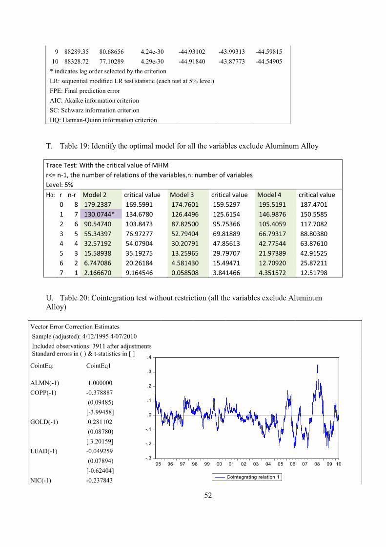
52

9 88289.35 80.68656 4.24e-30 -44.93102 -43.99313 -44.59815

10 88328.72 77.10289 4.29e-30 -44.91840 -43.87773 -44.54905

* indicates lag order selected by the criterion

LR: sequential modified LR test statistic (each test at 5% level)

FPE: Final prediction error

AIC: Akaike information criterion

SC: Schwarz information criterion

HQ: Hannan-Quinn information criterion T. Table 19: Identify the optimal model for all the variables exclude Aluminum Alloy Trace Test: With the critical value of MHM r<= n-1, the number of relations of the variables,n: number of variables Level: 5% H0: r n-r Model 2 critical value Model 3 critical value Model 4 critical value 0 8 179.2387 169.5991 174.7601 159.5297 195.5191 187.4701 1 7 130.0744* 134.6780 126.4496 125.6154 146.9876 150.5585 2 6 90.54740 103.8473 87.82500 95.75366 105.4059 117.7082 3 5 55.34397 76.97277 52.79404 69.81889 66.79317 88.80380 4 4 32.57192 54.07904 30.20791 47.85613 42.77544 63.87610 5 3 15.58938 35.19275 13.25965 29.79707 21.97389 42.91525 6 2 6.747086 20.26184 4.581430 15.49471 12.70920 25.87211 7 1 2.166670 9.164546 0.058508 3.841466 4.351572 12.51798

U. Table 20: Cointegration test without restriction (all the variables exclude Aluminum Alloy)

Vector Error Correction Estimates

Sample (adjusted): 4/12/1995 4/07/2010

Included observations: 3911 after adjustments Standard errors in ( ) & t-statistics in [ ]

CointEq: CointEq1

ALMN(-1)

1.000000

COPP(-1) -0.378887

(0.09485)

[-3.99458]

GOLD(-1) 0.281102

(0.08780)

[ 3.20159]

LEAD(-1) -0.049259

(0.07894)

[-0.62404]

NIC(-1) -0.237843

-.3

-.2

-.1

.0

.1

.2

.3

.4

95 96 97 98 99 00 01 02 03 04 05 06 07 08 09 10

Cointegrating relation 1

53

(0.05579)

[-4.26292]

OILBRE(-1) 0.018052

(0.04682)

[ 0.38552]

TIN(-1) 0.073963

(0.08125)

[ 0.91031]

ZINC(-1) -0.018329

(0.06578)

[-0.27864]

C -4.204268

(0.45480)

[-9.24422]

Error Correction: D(ALMN) D(COPP) D(GOLD) D(LEAD) D(NIC) D(OILBRE) D(TIN D(ZINC)

CointEq1 -0.013500 -0.013384 -0.005451 -0.018606 -0.005043 -0.017266 -0.009580 -0.013229

(0.00258) (0.00345) (0.00202) (0.00403) (0.00461) (0.00447) (0.00317) (0.00361)

[-5.24193] [-3.87739] [-2.70396] [-4.61153] [-1.09515] [-3.86042] [-3.02158] [-3.66109]

D(ALMN(-1)) 0.023528 -0.022226 0.010866 -0.019834 -0.040295 0.045981 -0.031292 0.029427

(0.02255) (0.03022) (0.01765) (0.03533) (0.04032) (0.03916) (0.02776) (0.03164)

[ 1.04336] [-0.73537] [ 0.61554] [-0.56142] [-0.99933] [ 1.17412] [-1.12718] [ 0.93008]

D(ALMN(-2)) -0.009412 0.052195 -0.043481 -0.018559 0.011421 0.103786 0.002899 0.011482

(0.02253) (0.03020) (0.01764) (0.03530) (0.04029) (0.03913) (0.02774) (0.03162)

[-0.41766] [ 1.72819] [-2.46503] [-0.52573] [ 0.28345] [ 2.65211] [ 0.10449] [ 0.36316]

D(COPP(-1)) -0.010816 -0.001947 0.041635 -0.047053 -0.051280 0.019502 -0.039663 -0.038261

(0.01859) (0.02492) (0.01455) (0.02913) (0.03324) (0.03229) (0.02289) (0.02608)

[-0.58177] [-0.07815] [ 2.86095] [-1.61553] [-1.54261] [ 0.60404] [-1.73298] [-1.46679]

D(COPP(-2)) -0.053460 -0.085709 -0.001905 -0.047591 -0.031557 -0.035578 -0.036393 -0.065720

(0.01857) (0.02489) (0.01454) (0.02909) (0.03320) (0.03225) (0.02286) (0.02605)

[-2.87898] [-3.44381] [-0.13104] [-1.63597] [-0.95042] [-1.10327] [-1.59201] [-2.52252]

D(GOLD(-1)) -0.001403 -0.087646 -0.019095 -0.022630 0.003799 -0.019255 -0.018525 -0.067656

(0.02151) (0.02882) (0.01683) (0.03369) (0.03845) (0.03735) (0.02647) (0.03017)

[-0.06525] [-3.04076] [-1.13429] [-0.67169] [ 0.09880] [-0.51558] [-0.69974] [-2.24224]

D(GOLD(-2)) 0.026610 0.029291 0.022363 0.000992 -0.002126 0.008332 -0.008884 0.022735

(0.02143) (0.02872) (0.01678) (0.03357) (0.03832) (0.03722) (0.02638) (0.03007)

[ 1.24164] [ 1.01976] [ 1.33305] [ 0.02954] [-0.05549] [ 0.22386] [-0.33675] [ 0.75611]

D(LEAD(-1)) -0.013211 0.002842 0.013253 0.085357 -0.035016 0.036240 -0.008544 0.008919

(0.01338) (0.01793) (0.01047) (0.02095) (0.02392) (0.02323) (0.01647) (0.01877)

[-0.98764] [ 0.15850] [ 1.26578] [ 4.07335] [-1.46404] [ 1.56011] [-0.51889] [ 0.47524]

D(LEAD(-2)) 0.000694 0.006379 0.016041 -0.025423 0.012689 -0.016496 0.021533 0.033662

(0.01339) (0.01795) (0.01048) (0.02098) (0.02394) (0.02326) (0.01649) (0.01879)

[ 0.05181] [ 0.35541] [ 1.53032] [-1.21186] [ 0.52993] [-0.70934] [ 1.30623] [ 1.79164]

D(NIC(-1)) 0.008103 0.000128 -0.001940 -0.003081 0.045474 0.018939 0.052526 -0.010300

(0.01137) (0.01524) (0.00890) (0.01782) (0.02033) (0.01975) (0.01400) (0.01596)

[ 0.71251] [ 0.00838] [-0.21797] [-0.17292] [ 2.23634] [ 0.95897] [ 3.75193] [-0.64552]

54

D(NIC(-2)) -0.004527 -0.006527 -0.000243 0.003414 -0.036213 0.008190 -0.014613 -0.016393

(0.01138) (0.01526) (0.00891) (0.01783) (0.02035) (0.01977) (0.01401) (0.01597)

[-0.39769] [-0.42779] [-0.02728] [ 0.19145] [-1.77914] [ 0.41431] [-1.04276] [-1.02638]

D(OILBRE(-1)) 0.003069 -0.002347 0.005067 -0.003718 0.025568 -0.005278 0.000231 0.004464

(0.00957) (0.01282) (0.00749) (0.01499) (0.01711) (0.01661) (0.01178) (0.01342)

[ 0.32079] [-0.18302] [ 0.67670] [-0.24805] [ 1.49476] [-0.31770] [ 0.01962] [ 0.33262]

D(OILBRE(-2)) 0.018092 0.011630 0.000932 -0.016405 0.022283 -0.011634 0.026724 0.007167

(0.00956) (0.01282) (0.00748) (0.01498) (0.01710) (0.01661) (0.01177) (0.01342)

[ 1.89209] [ 0.90746] [ 0.12447] [-1.09512] [ 1.30332] [-0.70063] [ 2.27030] [ 0.53419]

D(TIN(-1)) -0.016438 0.000104 -0.010530 0.018098 -0.002989 -0.015019 0.026860 -0.024335

(0.01519) (0.02036) (0.01189) (0.02380) (0.02716) (0.02638) (0.01870) (0.02131)

[-1.08203] [ 0.00512] [-0.88546] [ 0.76045] [-0.11005] [-0.56927] [ 1.43622] [-1.14169]

D(TIN(-2)) 0.036085 0.041036 -0.004811 0.027979 0.013627 0.009045 -0.019876 0.033844

(0.01517) (0.02033) (0.01187) (0.02376) (0.02712) (0.02634) (0.01867) (0.02128)

[ 2.37928] [ 2.01878] [-0.40525] [ 1.17758] [ 0.50248] [ 0.34341] [-1.06457] [ 1.59047]

D(ZINC(-1)) -0.037307 -0.033332 0.006465 -0.033685 0.014808 -0.051339 0.001069 -0.003805

(0.01685) (0.02259) (0.01319) (0.02641) (0.03014) (0.02927) (0.02075) (0.02365)

[-2.21341] [-1.47550] [ 0.49002] [-1.27570] [ 0.49135] [-1.75392] [ 0.05152] [-0.16089]

D(ZINC(-2)) 0.007365 0.001322 0.005593 0.016528 0.005021 -0.022479 -0.003205 -0.019447

(0.01685) (0.02259) (0.01319) (0.02640) (0.03014) (0.02927) (0.02075) (0.02365)

[ 0.43697] [ 0.05851] [ 0.42398] [ 0.62599] [ 0.16661] [-0.76804] [-0.15446] [-0.82243]

R-squared 0.015999 0.013911 0.014165 0.013152 0.005337 0.007921 0.010908 0.011145

Adj. R-squared 0.011956 0.009859 0.010114 0.009097 0.001250 0.003845 0.006844 0.007082

Sum sq. resids 0.662139 1.189434 0.405716 1.625056 2.116984 1.996925 1.003469 1.303446

S.E. equation 0.013040 0.017477 0.010207 0.020428 0.023316 0.022646 0.016053 0.018296

F-statistic 3.957064 3.433317 3.496933 3.243408 1.305909 1.943179 2.684006 2.742946

Log likelihood 11431.76 10286.31 12389.60 9676.066 9158.934 9273.104 10618.77 10107.31

Akaike AIC -5.837257 -5.251501 -6.327080 -4.939436 -4.674986 -4.733369 -5.421515 -5.159967

Schwarz SC -5.809996 -5.224240 -6.299819 -4.912175 -4.647725 -4.706109 -5.394254 -5.132706

Mean dependent 5.93E-05 0.000254 0.000275 0.000340 0.000312 0.000387 0.000293 0.000213

S.D. dependent 0.013119 0.017564 0.010259 0.020522 0.023331 0.022689 0.016108 0.018361

Determinant resid covariance (dof adj.) 3.91E-30

Determinant resid covariance 3.77E-30

Log likelihood 88088.43

Akaike information criterion -44.97235

Schwarz criterion -44.73983

55

V. Table 21: Weakly Exogeneity Test (all the variables exclude Aluminum Alloy) prob. a(1,1)=0 0.003679 a(2,1)=0 0.011661 a(3,1)=0 0.028243 a(4,1)=0 0.007364 a(5,1)=0 0.459552 a(6,1)=0 0.010844 a(7,1)=0 0.091410 a(8,1)=0 0.034469

W. Table 22: Cointegration test with restriction (all the variables exclude Aluminum Alloy)

Vector Error Correction Estimates

Sample (adjusted): 4/12/1995 4/07/2010

Included observations: 3911 after adjustments

Standard errors in ( ) & t-statistics in [ ]

Cointegration Restrictions: A(5,1)=0, A(7,1)=0, B(1,1)=1

Convergence achieved after 19 iterations.

Restrictions identify all cointegrating vectors

LR test for binding restrictions (rank = 1):

Chi-square(2) 2.871761

Probability 0.237906

Cointegrating Eq: CointEq1

ALMN(-1) 1.000000

COPP(-1) -0.504197

(0.08165)

[-6.17504]

GOLD(-1) 0.410922

(0.07558)

[ 5.43676]

LEAD(-1) 0.023726

(0.06795)

[ 0.34915]

NICKEl(-1) -0.121061

(0.04803)

[-2.52058]

OILBRE(-1) -0.038550

(0.04031)

[-0.95636]

TIN(-1) -0.056756

-.3

-.2

-.1

.0

.1

.2

.3

95 96 97 98 99 00 01 02 03 04 05 06 07 08 09 10

Cointegrating relation 1

56

(0.06994)

[-0.81145]

ZINC(-1) 0.008392

(0.05663)

[ 0.14820]

C -4.389347

(0.39151)

[-11.2114]

Error Correction: D(ALMN) D(COPP) D(GOLD) D(LEAD) D(NIC) D(OILBRE) D(TIN) D(ZINC)

CointEq1 -0.015005 -0.009304 -0.005781 -0.016617 0.000000 -0.013998 0.000000 -0.013613

(0.00260) (0.00329) (0.00236) (0.00416) (0.00000) (0.00524) (0.00000) (0.00358)

[-5.76092] [-2.82664] [-2.45298] [-3.99135] [ NA] [-2.67189] [ NA] [-3.80358]

D(ALMN(-1)) 0.024100 -0.024208 0.010947 -0.020992 -0.042393 0.043875 -0.034942 0.029655

(0.02256) (0.03027) (0.01766) (0.03537) (0.04034) (0.03921) (0.02780) (0.03166)

[ 1.06817] [-0.79979] [ 0.61986] [-0.59342] [-1.05080] [ 1.11887] [-1.25682] [ 0.93673]

D(ALMN(-2)) -0.008640 0.050125 -0.043335 -0.019659 0.009138 0.101618 -0.001065 0.011868

(0.02255) (0.03025) (0.01765) (0.03535) (0.04032) (0.03919) (0.02779) (0.03164)

[-0.38315] [ 1.65697] [-2.45513] [-0.55607] [ 0.22664] [ 2.59283] [-0.03834] [ 0.37511]

D(COPP(-1)) -0.011887 -0.001106 0.041314 -0.047076 -0.049954 0.020251 -0.037394 -0.039062

(0.01861) (0.02496) (0.01456) (0.02917) (0.03327) (0.03234) (0.02293) (0.02611)

[-0.63888] [-0.04429] [ 2.83669] [-1.61374] [-1.50150] [ 0.62623] [-1.63098] [-1.49623]

D(COPP(-2)) -0.054748 -0.085080 -0.002313 -0.047911 -0.030310 -0.035104 -0.034274 -0.066733

(0.01859) (0.02493) (0.01455) (0.02914) (0.03323) (0.03230) (0.02290) (0.02608)

[-2.94574] [-3.41223] [-0.15900] [-1.64416] [-0.91202] [-1.08670] [-1.49654] [-2.55894]

D(GOLD(-1)) 0.000910 -0.086605 -0.018234 -0.020398 0.003527 -0.017691 -0.018878 -0.065553

(0.02152) (0.02887) (0.01684) (0.03374) (0.03848) (0.03740) (0.02652) (0.03019)

[ 0.04230] [-2.99990] [-1.08247] [-0.60456] [ 0.09166] [-0.47300] [-0.71191] [-2.17099]

D(GOLD(-2)) 0.029222 0.030880 0.023359 0.003827 -0.002058 0.010558 -0.008623 0.025164

(0.02144) (0.02877) (0.01678) (0.03362) (0.03834) (0.03727) (0.02642) (0.03009)

[ 1.36284] [ 1.07350] [ 1.39173] [ 0.11385] [-0.05367] [ 0.28331] [-0.32637] [ 0.83639]

D(LEAD(-1)) -0.011883 0.004698 0.013821 0.087599 -0.034029 0.038539 -0.006742 0.010290

(0.01337) (0.01794) (0.01046) (0.02096) (0.02391) (0.02324) (0.01647) (0.01876)

[-0.88888] [ 0.26196] [ 1.32067] [ 4.17909] [-1.42348] [ 1.65858] [-0.40924] [ 0.54854]

D(LEAD(-2)) 0.002147 0.008327 0.016658 -0.023032 0.013692 -0.014072 0.023372 0.035152

(0.01338) (0.01795) (0.01048) (0.02098) (0.02393) (0.02326) (0.01649) (0.01878)

[ 0.16046] [ 0.46378] [ 1.59005] [-1.09762] [ 0.57212] [-0.60497] [ 1.41718] [ 1.87190]

D(NIC(-1)) 0.009397 0.001250 -0.001427 -0.001420 0.045812 0.020415 0.053189 -0.009052

(0.01137) (0.01526) (0.00890) (0.01783) (0.02034) (0.01977) (0.01401) (0.01596)

[ 0.82628] [ 0.08194] [-0.16031] [-0.07961] [ 2.25274] [ 1.03281] [ 3.79536] [-0.56727]

D(NIC(-2)) -0.003335 -0.005472 0.000231 0.004960 -0.035883 0.009574 -0.013969 -0.015241

(0.01138) (0.01527) (0.00891) (0.01785) (0.02036) (0.01979) (0.01403) (0.01597)

[-0.29296] [-0.35828] [ 0.02591] [ 0.27791] [-1.76277] [ 0.48386] [-0.99578] [-0.95416]

D(OILBRE(-1)) 0.002893 -0.001897 0.005033 -0.003483 0.026069 -0.004808 0.001099 0.004374

(0.00957) (0.01284) (0.00749) (0.01500) (0.01711) (0.01663) (0.01179) (0.01343)

[ 0.30236] [-0.14776] [ 0.67193] [-0.23217] [ 1.52355] [-0.28910] [ 0.09324] [ 0.32575]

57

D(OILBRE(-2)) 0.017998 0.012166 0.000930 -0.016054 0.022819 -0.011055 0.027659 0.007156

(0.00956) (0.01283) (0.00749) (0.01500) (0.01710) (0.01662) (0.01179) (0.01342)

[ 1.88186] [ 0.94816] [ 0.12428] [-1.07063] [ 1.33431] [-0.66502] [ 2.34693] [ 0.53327]

D(TIN(-1)) -0.015984 0.000384 -0.010356 0.018594 -0.002974 -0.014628 0.026911 -0.023913

(0.01519) (0.02038) (0.01189) (0.02382) (0.02717) (0.02641) (0.01872) (0.02132)

[-1.05204] [ 0.01883] [-0.87078] [ 0.78052] [-0.10948] [-0.55392] [ 1.43736] [-1.12164]

D(TIN(-2)) 0.036550 0.041391 -0.004629 0.028539 0.013703 0.009521 -0.019717 0.034286

(0.01517) (0.02035) (0.01187) (0.02378) (0.02712) (0.02636) (0.01869) (0.02128)

[ 2.40970] [ 2.03402] [-0.38991] [ 1.20000] [ 0.50523] [ 0.36114] [-1.05487] [ 1.61093]

D(ZINC(-1)) -0.038152 -0.033849 0.006143 -0.034604 0.014784 -0.052062 0.000980 -0.004591

(0.01686) (0.02262) (0.01320) (0.02643) (0.03014) (0.02930) (0.02077) (0.02365)

[-2.26314] [-1.49667] [ 0.46551] [-1.30920] [ 0.49043] [-1.77683] [ 0.04719] [-0.19407]

D(ZINC(-2)) 0.006383 0.000752 0.005221 0.015483 0.005020 -0.023285 -0.003259 -0.020356

(0.01686) (0.02261) (0.01320) (0.02643) (0.03014) (0.02930) (0.02077) (0.02365)

[ 0.37867] [ 0.03327] [ 0.39565] [ 0.58582] [ 0.16655] [-0.79475] [-0.15688] [-0.86063]

R-squared 0.015803 0.011804 0.013950 0.011311 0.005046 0.006048 0.008771 0.010773

Adj. R-squared 0.011759 0.007743 0.009899 0.007248 0.000958 0.001964 0.004698 0.006709

Sum sq. resids 0.662271 1.191975 0.405804 1.628088 2.117604 2.000695 1.005637 1.303935

S.E. equation 0.013041 0.017496 0.010208 0.020448 0.023320 0.022667 0.016070 0.018299

F-statistic 3.907755 2.907074 3.443158 2.784200 1.234272 1.480941 2.153419 2.650539

Log likelihood 11431.37 10282.14 12389.18 9672.422 9158.362 9269.416 10614.55 10106.58

Akaike AIC -5.837058 -5.249366 -6.326862 -4.937572 -4.674693 -4.731483 -5.419356 -5.159591

Schwarz SC -5.809797 -5.222106 -6.299601 -4.910311 -4.647432 -4.704223 -5.392096 -5.132331

Mean dependent 5.93E-05 0.000254 0.000275 0.000340 0.000312 0.000387 0.000293 0.000213

S.D. dependent 0.013119 0.017564 0.010259 0.020522 0.023331 0.022689 0.016108 0.018361

Determinant resid covariance (dof adj.) 3.91E-30

Determinant resid covariance 3.78E-30

Log likelihood 88086.99

Akaike information criterion -44.97162

Schwarz criterion -44.73910

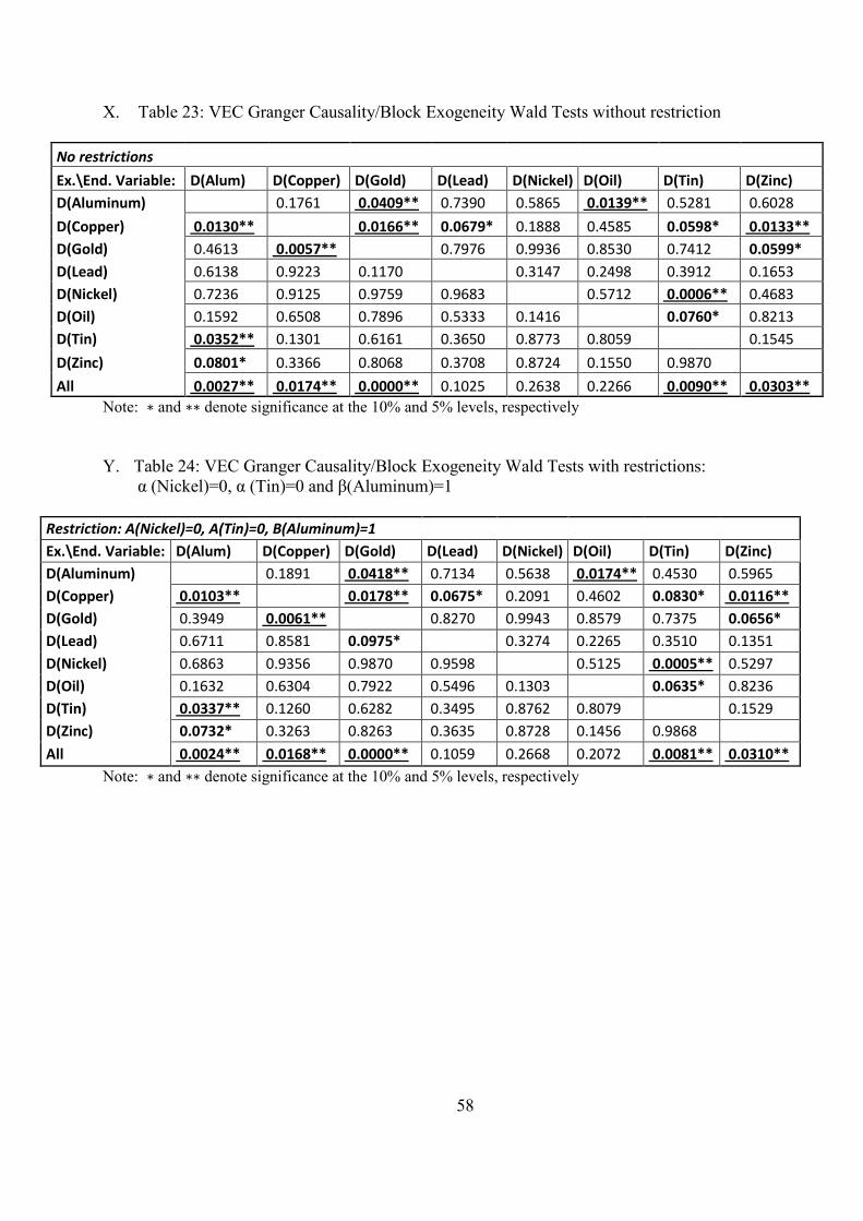
58

X. Table 23: VEC Granger Causality/Block Exogeneity Wald Tests without restriction

No restrictions

Ex.\End. Variable: D(Alum) D(Copper) D(Gold) D(Lead) D(Nickel) D(Oil) D(Tin) D(Zinc) D(Aluminum) 0.1761 0.0409** 0.7390 0.5865 0.0139** 0.5281 0.6028

D(Copper) 0.0130** 0.0166** 0.0679* 0.1888 0.4585 0.0598* 0.0133** D(Gold) 0.4613 0.0057** 0.7976 0.9936 0.8530 0.7412 0.0599* D(Lead) 0.6138 0.9223 0.1170 0.3147 0.2498 0.3912 0.1653 D(Nickel) 0.7236 0.9125 0.9759 0.9683 0.5712 0.0006** 0.4683 D(Oil) 0.1592 0.6508 0.7896 0.5333 0.1416 0.0760* 0.8213 D(Tin) 0.0352** 0.1301 0.6161 0.3650 0.8773 0.8059 0.1545

D(Zinc) 0.0801* 0.3366 0.8068 0.3708 0.8724 0.1550 0.9870

All 0.0027** 0.0174** 0.0000** 0.1025 0.2638 0.2266 0.0090** 0.0303** Note: � and �� denote significance at the 10% and 5% levels, respectively Y. Table 24: VEC Granger Causality/Block Exogeneity Wald Tests with restrictions: α (Nickel)=0, α (Tin)=0 and β(Aluminum)=1

Restriction: A(Nickel)=0, A(Tin)=0, B(Aluminum)=1 Ex.\End. Variable: D(Alum) D(Copper) D(Gold) D(Lead) D(Nickel) D(Oil) D(Tin) D(Zinc) D(Aluminum) 0.1891 0.0418** 0.7134 0.5638 0.0174** 0.4530 0.5965 D(Copper) 0.0103** 0.0178** 0.0675* 0.2091 0.4602 0.0830* 0.0116** D(Gold) 0.3949 0.0061** 0.8270 0.9943 0.8579 0.7375 0.0656* D(Lead) 0.6711 0.8581 0.0975* 0.3274 0.2265 0.3510 0.1351 D(Nickel) 0.6863 0.9356 0.9870 0.9598 0.5125 0.0005** 0.5297 D(Oil) 0.1632 0.6304 0.7922 0.5496 0.1303 0.0635* 0.8236 D(Tin) 0.0337** 0.1260 0.6282 0.3495 0.8762 0.8079 0.1529 D(Zinc) 0.0732* 0.3263 0.8263 0.3635 0.8728 0.1456 0.9868 All 0.0024** 0.0168** 0.0000** 0.1059 0.2668 0.2072 0.0081** 0.0310**

Note: � and �� denote significance at the 10% and 5% levels, respectively