LIVING WITH THE TRILEMMA CONSTRAINT: …web.pdx.edu/~ito/w19448.pdfLiving with the Trilemma...

NBER WORKING PAPER SERIES

LIVING WITH THE TRILEMMA CONSTRAINT: RELATIVE TRILEMMA POLICY DIVERGENCE, CRISES, AND OUTPUT LOSSES FOR DEVELOPING COUNTRIES

Joshua AizenmanHiro Ito

Working Paper 19448http://www.nber.org/papers/w19448

NATIONAL BUREAU OF ECONOMIC RESEARCH1050 Massachusetts Avenue

Cambridge, MA 02138September 2013

The views expressed herein are those of the authors and do not necessarily reflect the views of theNational Bureau of Economic Research.The financial support of faculty research funds of PortlandState University is gratefully acknowledged

NBER working papers are circulated for discussion and comment purposes. They have not been peer-reviewed or been subject to the review by the NBER Board of Directors that accompanies officialNBER publications.

© 2013 by Joshua Aizenman and Hiro Ito. All rights reserved. Short sections of text, not to exceedtwo paragraphs, may be quoted without explicit permission provided that full credit, including © notice,is given to the source.

Living with the Trilemma Constraint: Relative Trilemma Policy Divergence, Crises, and OutputLosses for Developing CountriesJoshua Aizenman and Hiro ItoNBER Working Paper No. 19448September 2013JEL No. F31,F36,F41,O24

ABSTRACT

This paper investigates the potential impacts of the degree of divergence in open macroeconomicpolicies in the context of the trilemma hypothesis. Using an index that measures the relative policydivergence among the three trilemma policy choices, namely monetary independence, exchangerate stability, and financial openness, we find that emerging market countries have adopted trilemmapolicy combinations with the least degree of relative policy divergence in the last fifteen years. We alsofind that a developing or emerging market country with a higher degree of relative policy divergenceis more likely to experience a currency or debt crisis. However, a developing or emerging marketcountry with a higher degree of relative policy divergence tends to experience smaller output losseswhen it experiences a currency or banking crisis. Latin American crisis countries tended to reducetheir financial integration in the aftermath of a crisis, while this is not the case for the Asian crisiscountries. The Asian crisis countries tended to reduce the degree of relative policy divergence in theaftermath of the crisis, probably aiming at macroeconomic policies that are less prone to crises. Thedegree of relative policy divergence is affected by past crisis experiences – countries that experiencedcurrency crisis or a currency-banking twin crisis tend to adopt a policy combination with a smallerdegree of policy divergence.

Joshua AizenmanEconomics and SIRUSCUniversity ParkLos Angeles, CA 90089-0043and [email protected]

Hiro ItoPortland State University1721 SW Broadway, Suite 241Portland, Oregon [email protected]

1

1. Introduction

Managing policies in an economic turbulence is a challenging task, especially when the world economy is highly integrated and markets are intertwined with each other. History is full of episodes where monetary regimes ends abruptly, as we have witnessed in the collapse of the Bretton Woods system in the early 1970s or in the financial crises many emerging market economies experienced in the 1980s and 1990s. These abrupt endings of regimes often involve crises or some sort of financial turbulence. No matter what forms of international monetary systems or regimes replace the old ones, countries end up adopting a combination of three policy goals: monetary independence, exchange rate stability, and financial openness, with different degrees of attainment in each. That is, a powerful hypothesis called the “impossible trinity,” or the “trilemma” dictates open macro policy management. Countries may choose any two, but not all, of the three policy goals to their full extent, or adopt a combination of intermediate degrees of all of the three policy goals.

Theory and empirical evidence tell us that each one of the three trilemma policy choices can be a double-edged sword as recognized by a significant amount of recent literature.1 To make the matter more complicated, the effect of each policy choice can differ depending on what other policy choice it is paired with. For example, exchange rate stability can be destabilizing when paired with financial openness, yet be stabilizing if paired with greater monetary autonomy.

Furthermore, countries rarely face the stark polarized binary choices as often envisioned by policy makers and researchers. In Mundell’s (1963) textbook trilemma triangle, portrayed in Figure 1, each of the three sides represents the full implementation of each of the three policy goals. We can locate the Euro system or the gold standard at the corner that represents the full attainment of financial openness and exchange rate stability while the Bretton Woods system can be placed at the corner of full exchange rate stability and full monetary independence. When a country adopts a policy combination of intermediate levels for all the three policy choices, such a policy combination would be located somewhere inside the trilemma triangle. Intriguingly, measuring empirically the three policy trilemma choices, their weighted sum adds up, statistically, to a constant [see Aizenman, et al. (2012) and Ito and Kawai (2012)]. Thus, achieving a higher trilemma policy goal is traded off by a drop in the weighted sum of the other two trilemma policies. Obviously, different combinations of the three policies have different macroeconomic effects. A key question is, how can the location of a country’s policy combination in the trilemma triangle affect its macroeconomic performance, especially in terms of avoiding traumatic economic turbulence such as financial crises?

Against this backdrop, we first construct a metric that measures the degree of divergence among the three trilemma policies relative to the global trend. With this index, we evaluate the patterns of divergence of trilemma policy combinations in the last four decades. In Section 3, we

1 As for monetary independence, refer to Obstfeld, et al. (2005), Shambaugh (2004), and Frankel et al. (2004). On the impact of the exchange rate regime, refer to Ghosh et al. (1997), Levy-Yeyati and Sturzenegger (2003), and Eichengreen and Leblang (2003). The empirical literature on the effect of financial liberalization is surveyed by Henry (2006), Kose et al. (2006), Prasad et al. (2003), and Prasad and Rajan (2008).

2

implement a series of empirical exercises to examine the impact of the degree of trilemma relative policy divergence on macroeconomic performance, namely the probability of the onset of a currency, banking, and debt crisis, and also the output losses from these different types of crises. We also compare the degree of relative policy divergence and trilemma policy arrangements in the Latin American crisis countries during 1980s and in the Asian crisis countries during the 1990s and identify commonalties and differences between these crisis periods. In Section 4, we focus on the endogenous nature of the degree of relative policy divergence and how it can be affected by past crisis experiences. In Section 5, we summarize the main findings of the paper.

2. Divergence of the Trilemma Policy Choices 2.1 Why Does the Extent of Relative Policy Divergence Matter?

While there are only three kinds of polarized policy combinations among the three trilemma policies, i.e., the three vertexes in the triangle in Figure 1, once intermediate levels for each policy are allowed, there can exist an infinite number of open macro policy combinations. Until recently, researchers have tended to focus on debating the merits and demerits of polarized monetary regimes. Fischer (2001) argued the unstable nature of intermediate exchange rate regimes, pointing out that such regimes are more prone to experience a crisis in a financially globalized world. Frankel (1999), while admitting that regimes with “corner solutions” can be simple and transparent in showing government commitment to maintaining a regime, argued that avoiding intermediate regimes is not always the best solution for countries, especially developing ones. Willett (2003) argued that the issue is not so much about whether polarized or intermediate regimes are more or less stable. Rather, that the issue of whether macroeconomic conditions of an economy are consistent with its monetary regime is more important. The crises that occurred among emerging market countries in the 1980s and 1990s, and the Global Financial Crisis of 2008-09 to a similar extent, have raised questions about the global trend of financial liberalization, leading researchers to debate the merits and demerits of greater financial openness.

Despite the debate, regimes with corner solutions are more of a rarity. In other words, most countries often operate “somewhere inside the triangle.” For example, some countries implement partial financial integration while trying to retain control over exchange rate movement as well as monetary policy autonomy. This sort of clustering of the three policies inside the trilemma triangle, or the “middle-ground convergence,” has been a characteristic of emerging market countries (EMG) in recent decades as Aizenman, Chinn, and Ito (2012) have shown. Aizenman, et al. have also found that in recent years such middle-ground convergence has been more evident among Asian EMGs.

By adopting such converged policy combinations, these countries may have been trying to dampen the negative effects that may arise from adopting polarized policy regimes. Interestingly, the period when EMG’s middle convergence started becoming more evident

3

coincides with the time when some of these economies began accumulating sizable international reserves (IR), probably trying to buffer the trade-off arising from the trilemma, again a more evident trend among Asian EMGs.2

A key question is how the location within the trilemma triangle affects macroeconomic performance, especially when we focus on the risk of experiencing a financial crisis. Before exploring this question, however, we need to raise another important issue. That is, even if certain open macro policy combinations were found to affect the likelihood of a country experiencing a crisis and its output cost, such correlations may not be merely a function of the country’s own macroeconomic policies.

A country’s open macro policies need to be evaluated in a greater context, compared with policies adopted by other countries. For example, a fixed exchange rate regime must have different effects on the economy depending on whether or not most other countries also adopt fixed exchange rate regimes as they did during the Bretton Woods period. As another example, the consequence of liberalizing the financial market by a country differ between the 1960s, when most countries had closed financial markets, and recent years when many countries have been moving toward full financial liberalization.

Anecdotally, countries tended to adopt monetary regimes prevalent in other countries, making the types of monetary regimes across countries correlated with each other. Such correlated behavior can be sometimes global as was the case of the Gold Standard during the pre-WWII era or the Bretton Woods system, other times regional such as the Euro system, or clustered around similar income levels such as the middle-ground convergence observed among emerging market economies in recent years. When many countries tend to adopt similar monetary regimes, such a herding behavior tends to create externalities, lowering the cost of a country following such a global or regional trend, or the “mean behavior.” Conversely, herding behavior in arranging monetary regimes may also raise the opportunity cost of deviating from it, unless the country that deviates from the “mean behavior” is well-equipped with healthy fundamentals or solid institutions including well-functioning financial markets. In this sense, one could argue that the pursuit of forming a monetary union by some European countries is more sustainable only if these countries are equipped with appropriate levels of institutional development and good fundamentals.3 Hence, it is important to evaluate the combinations of open macro policies in a global context or in comparison to other countries.

In this paper, we will focus particularly on the impact of a triad policy combination on the likelihood of a financial crisis as well as on the output losses once a financial crisis arises. By financial crisis, we mean three kinds of financial crises, namely currency, banking, and debt crises. While it may not be difficult to consider the relationship between the degrees of relative policy divergence and their impact on currency crisis, the link between them and their impact on

2 Aizenman, et al. (2010) empirically show that pursuing greater exchange stability can be increasing output volatility for developing economies, but that can be mitigated by holding a larger amount of international reserves than the threshold of about 20% of GDP. 3 Furthermore, it means the current crisis situation faced by some of the Euro countries can be explained by their weak fundamentals and institutional development.

4

banking or debt crises may not sound straightforward. However, both the probability of occurrence and the output losses of banking or debt crises can be direct functions of the triad policy coordination.

As for a banking crisis, the recent European experience makes it clear that a choice of a monetary regime can affect the likelihood and the cost of experiencing a banking crisis. In the case of the Euro crisis, participating in the monetary union had made it easier for certain countries such as Ireland, Spain, and Cyprus to experience a surge in capital flows in an unsustainable fashion. Such capital influx ended by sowing the seeds for the ongoing banking and debt crises in these countries. The situation could have been different and less costly if these countries had not participated in the fixed exchange rate arrangement, as it rids countries with highly open financial markets of monetary independence.

The debt crisis in emerging market economies during the 1980s and 1990s and in Southern Europe, including Greece, can be explained in the context of the trilemma. For emerging market economies, the predominant global trend for financial liberalization had converted the trilemma into the dilemma between pursuing greater monetary autonomy (with more flexible exchange rates) and greater exchange rate stability (with less monetary autonomy). Facing the “original sin” (Eichengreen and Hausmann, 1999), many emerging market economies had chosen the path of greater exchange rate stability while the inevitably weaker monetary independence made these economies more vulnerable to external shocks.

Thus, not only for currency crises, but also for banking and debt crises, how the three trilemma policies are coordinated by individual countries and where they stand in the global context can be an important factor.

2.2 Measure of relative policy divergence and Its Patterns

In order to gage how much convergence or divergence is taking place among the three trilemma policy choices in a global context, we construct the “measure of divergence” in the triad policies. For that, we use the “trilemma indexes” introduced by Aizenman, Chinn, and Ito (2010, 2012).

The trilemma indexes measure the degree of achievement in each of the three policy choices for more than 170 economies from 1970 through 2010.4 The monetary independence index (MI) is based on the correlation of a country’s interest rates with the base country’s interest rate. The index for exchange rate stability (ERS) is an invert of exchange rate volatility, i.e., standard deviations of the monthly rate of depreciation, using the exchange rate between the home and base economies. The degree of financial integration is measured by the Chinn-Ito (2006, 2008) capital controls index (KAOPEN). 5

Using these indexes, we define the “measure of relative policy divergence” as below:

_ 1 _ 1 _ 1 (1)

4 The indexes are available at http://web.pdx.edu/~ito/trilemma_indexes.htm. 5 Refer to Aizenman, et al. (2012), and the Trilemma website for the details of construction of the indexes.

5

where _ for X = MI, ERS, and KAOPEN, and is cross-country average of X in year

t.6,7 By definition, is a geometric mean of three dimensions of the Trilemma variable of country i at time t from the prevailing average choices, reflecting the relative divergence of the country’s policies from the vector , , > Long-run Trends

Figure 2 illustrates the average of dit for different subgroups of countries based on income levels. We can make several interesting observations based on this figure. For the last two decades, advanced economies tended to have two combinations of distinctive policies. The Euro country group has the highest degree of relative policy divergence among the country groups (opting for high degrees of exchange rate stability and financial integration), followed by the group of non-Euro advanced economies (opting for high degrees of monetary independence and financial integration). Higher income countries may be able to afford to have divergent policy combinations.

The group of emerging market economies has had the lowest degree of policy divergence in the last two decades. Since the beginning of the 1980s, developing economies, whether or not emerging markets, have had relatively stable movement in the degree of policy convergence except for the mid-1990s when both subgroups of developing economies experienced a drop in the degree of policy divergence. During the crisis years of 1982 (the debt crisis), 1997-98 (the Asian financial crisis), and 2008-09 (the global financial crisis), the policy convergence measure tends to rise around the times of the crises.8

It would be interesting to see if there are any regional characteristics in the formation of triad open macro policies. As we have discussed, externality can play a role in concerting policy decision makings among neighboring countries in a region, while possibly increasing the cost of shying away from regional policy coordination. Furthermore, there can be a regional economic integration such as in the case of the East Asian supply chain network or a monetary policy arrangement as in the case of the Gulf Cooperation Council (GCC). Hence, a comparison among geographical groups of countries should shed light on the differences in the characteristics of

6 The cross country average ( tX )

is the sample average of X including both industrialized and developing countries

for year t. 7 One could argue that if the extent of the three trilemma policy choices are linearly related as theoretically predicted, the above formula for d does not have to contain all the three indexes – it would need only any two of the three trilemma indexes. However, we do not assume the linearity too strictly, i.e., the linearity does not have to hold every single year. In other words, we assume that there is some room for policy choices to deviate from the trilemma constraint. In fact, policy makers sometimes intentionally or unintentionally challenge the constraint of the trilemma by implementing a policy combination that is not consistent with the trilemma hypothesis. Before aborting the fixed exchange rate arrangement for the Thai baht, Thai policy makers attempted to challenge the trilemma by pursuing both greater monetary independence and exchange rate stability without imposing capital controls. Also, holding a massive amount of IR may allow countries to deviate from the constraint of the trilemma in the short run. 8 To see what is driving the trajectories in Figure 2, looking at the group mean of the ratios of each of the three indexes to its cross-country mean (i.e.,

t

it

XX with X for monetary policy independence (MI), exchange rate stability

(ERS), and financial openness (KAOPEN)) is helpful. For that, refer to Aizenman and Ito (2012).

6

triad open macro policies among countries. Figure 3 illustrates the averages of the policy dispersion measure (dit) for different regional country groups, focusing on Latin American and Asian economies.

Interestingly, since the late 1990s, a period coinciding with the Asian Crisis period, the degree of relative policy divergence has been persistently small among all regional groups.9 This policy convergence among developing economies may reflect the great moderation, but the convergence seems to be still in place in the last few years of the sample, coinciding with the years of the global financial crisis. Additionally, despite their high levels of relative policy divergence in the 1980s, emerging market economies in Asia have been experiencing lowest levels of relative policy divergence in the last decade.10 Behavior of d around the Time of a Crisis

Let us observe the behavior of the measure of policy dispersion around the time of a financial crisis. Figures 4-6 show the development of the cross-country average of the degree of relative policy divergence (d) for different subsamples of countries for currency, banking, and debt crises, respectively.11 The average of the relative policy divergence measure across countries that experiences a particular type of crisis is illustrated over the period from three years before the first year of the crisis through three years after it (i.e., [t0 – 3, t0 + 3]). In each figure, Panel (a) shows the development of the subsample averages of d for IDC, LDC, and EMG.12 Panel (b) shows the development of the averages of d for the crisis countries that experienced positive output losses as a result of a crisis (top), and those which experienced output gains (i.e., output losses < 0) (bottom).13 Panel (c) compares the development of the d for the crisis countries with “high” IR holdings with those with “low” IR holdings, while “high” IR holdings means that the level of IR holdings (as a share of GDP) is higher than the annual cross-country median (of all the countries in the entire sample, including crisis and non-crisis economies) as of the year before the crisis occurrence (t0 – 1).

In all three kinds of crises, there is a hump shape of development for d around the first year of the crisis, while the peak occurs at the first year for currency crisis (t0); a year after the onset of a banking crisis (t0+1); and a year before the onset of a debt crisis (t0+1). In the cases of

9 This is also true for the group of middle-eastern or North African countries (not reported). 10 Asian emerging market economies (and countries in the middle-east, though not reported) experienced high levels of relative policy divergence from the beginning of the 1980s through the early 1990s. This is partly because Latin American countries, many of which went through debt crises, retrenched financial openness around the same period, dragging down the average and making the financial liberalization efforts by Asian emerging market countries especially distinctive. 11 The methods for identifying the three types of crises are explained in Appendix 1. 12 The emerging market countries (EMGs) are defined as the countries classified as either emerging or frontier during the period of 1980-1997 by the International Financial Corporation plus Hong Kong and Singapore. 13 As we explain later, output losses are defined as the cumulative sum of the differences between actual and trend real GDP over the four-year period (i.e., [t0, t0+3]. The trend real GDP is based on HP-filtered real GDP series over the twenty-year-long pre-crisis period [t0 – 20, t0 – 1]. Based on whether the cumulative sum is positive or negative, a crisis is defined to involve output losses or gains. In a sense, the existence of output losses is based on “output losses in ex post,” not strictly as of the first year of the crisis.

7

currency and banking crises, if the crisis involves output losses, the measure of relative policy divergence tends to stay at high levels during the first and second years of the crisis. In the case of the debt crisis, countries that did not experience output losses, experience a peak in d in the year before the onset of the crisis. This may imply that these countries could avoid output losses by preemptively implementing stabilization measures that end up raising the degree of policy divergence.

For the currency or banking crisis countries, if they hold low levels of IR, there is a distinct rise in d at the onset of the crisis and a distinct fall afterwards. If these countries are high IR holders, the peak occurs in the second year of the crisis. This generalization is more apparent for the high IR holding countries with output losses (not reported). These findings may suggest that if a country experiences a currency or banking crisis without holding high levels of IR, the country needs to implement policies that raise d, whereas d would rise more slowly for high IR holders.

It is harder to generalize the movement of d for debt crisis countries. Panel (c) shows that holding higher levels of IR seems to allow a crisis country to raise d prior to the onset of a crisis. However, those debt crisis countries that experience a peak in d prior to the onset of a crisis tend to be the ones that experience output losses, which tend to be contrary to the case of currency or banking crises countries. Those with high IR holdings tend to lower the level of d around the time of the crisis, unlike among currency or banking crisis countries.

There is a limit to what one can infer from observing unconditional means of the measure of relative policy divergence around the time of a crisis. Furthermore, while d can be a policy variable, it can be also endogenously affected by the development of general economic conditions. These issues are important especially when one looks into the relationship between d and the crisis. In order to deal with these issues, we continue with an econometric evaluation of the degree of relative policy divergence. Specifically, we examine the effect of policy divergence, d, on the probability of crisis onsets, and whether and to what extent policy divergence influences the size of output losses that arise with the crises.

3. Empirical Analysis 3.1 Probability of Crisis Occurrence

We first estimate the probability of different types of crises to examine whether and to what extent the degree of relative policy divergence affects the likelihood of a crisis occurrence. The crises we examine are: currency, banking, and debt crisis. The identification methods for each of the crises are explained in Appendix 1.

For each type of the crisis, we assign the value of one to a binary variable yt when country i experiences the onset of a crisis in year t, and zero, otherwise.14 We hypothesize the probability that a crisis will occur, Pr(yt = 1) is a function of a vector of characteristics associated with observations in year t, or Xt, and the parameter vector β, with the control variables in X

14 We only focus on the onset of a crisis, that is, the first year of the crisis. This means that we do not investigate the persistence of a crisis situation if it lasts longer than one year.

8

lagged one year to avoid endogeneity issues. Using the panel data composed of more than 100 countries for the period 1970 – 2010, the log of the following function is maximized with respect to the unknown parameters through non-linear maximum likelihood.

m

i tttt XFyXFyL1

'1ln1'lnln (2)

where m indicates the number of countries times the number of observations for each country and the function F(.) is the standardized normal distribution.

The following variables are included in the characteristics vector Xt. The choice of the variables is based on the past literature, except for the ones related to the degree of trilemma policy convergence. Variables included in the estimation:

Relative income to the U.S. – Countries’ per capita income levels from the Penn World Table (PWT) are normalized as a ratio to the U.S. per capita income level.

International reserves (IR) holding – IR excluding gold as a ratio to GDP .

Per capita Output growth – The growth rate of GDP per capita (in local currency).

Private credit growth – The change (first-difference) in the ratio of private credit creation to GDP.

Net Debt inflows – The ratio of (external debt liabilities– external debt assets) to GDP. The original data are from Lane and Milesi-Ferretti (2007 and updates).

Gross external financial exposure – The ratio of (total external assets + total external liabilities) to GDP, included as deviations from the five-year average of the ratios. After the global financial crisis, in addition to net capital flows or investment positions, gross capital flows have been pointed as potential destabilizing factors.15 The data are based on Lane and Milesi-Ferretti (2007 and updates).

Real exchange rate overvaluation – It is defined as deviations from a fitted trend in the real exchange rate. The real exchange rate is calculated using the exchange rate between country i and its base country (in the sense of Aizenman, et al., 2011), and the CPI of the two countries. Higher values of this variable indicate the real exchange rate value is lower, i.e., appreciated, than its time trend.

Exchange rate stability (ERS) and Financial openness (KAOPEN) – Both are from the trilemma indexes of Aizenman, Chinn, and Ito (2012).

15 See Borio and Disyatat (2011), Obstfeld (2012a, b), Bruno and Shin (2012) for the argument on how gross external financial exposure matters for financial and economic stability. However, it must be noted that gross external financial exposure may also mean a higher level of ability to diversify risk, which may work as a stabilizing fact.

9

Triad Relative policy divergence Measure – The aforementioned measure of triad relative policy divergence dit is included.

Standard deviations of the Triad Relative policy divergence Measure – The standard deviations of the above dit over five years from t–5 through t–1 are included to examine the impact of the stability level of the trilemma policy combinations.

Other crises – The dummies for the other types of crises that occur either concurrently (t) or in the previous year (t–1) are also included.

Contagion – To see the impact of other crises in the same geographical region, we also include a variable that represents the effect of regional contagion. The variable to be included is defined as:

K

K

P

ijj

ntij

nti CDContagion

1,, (3).

CDni,t is a crisis dummy for type n crisis (i.e., currency, banking, or debt).

kj is the

weight based on GDP in PPP for country j ( ij ) in region K. Hence, the variable Contagionn is

the weighted sum of the dummy variables for the countries in the region country i belongs to, excluding the weighted dummy of country i itself.16 The basic assumptions are that the more countries in the same geographical region experience crises, the more likely it is for country i to experience a crisis, and that the contagious effect is larger for bigger economies.

We apply the above probit estimation model to the full sample that includes both industrialized and developing countries, the sample of industrialized countries (IDC), the sample of developing countries (LDC), and a subsample of emerging market countries (EMG). The baseline estimation results are reported in Table 1, which reports the marginal effects of the explanatory variables assuming variables take mean values (except for the dummy variables).17,18 3.2 Estimation Results – The Determinants of Crisis Occurrences

We make observations of the estimations mainly for the samples of developing and emerging market economies.

16 The regions we consider are: West hemisphere (i.e., North and South Americans), East and Southeast Asia and the Pacific, South Asia, Europe (including both Western, Eastern, and Central Europe), and Sub-Saharan Africa, Middle East and North Africa. 17 The variables that are persistently insignificant and therefore dropped from the estimation include: trade openness measured by the sum of export and import values as a ratio to GDP; the dummy for countries’ engagement in both internal and external armed conflicts; the dummies for commodity exporters and manufacturing exporters; the degree of fiscal procyclicality, which is measured by the correlation between HP-detrended output and government expenditure; the dummy for the existence of the deposit insurance; volatility of the TOT income shocks; and the dummy for hyperinflation (with the annual rate of inflation exceeding 40%). 18 In the estimation for debt crisis, the estimation results for the full or IDC sample are not reported because there is no debt crisis data for industrialized countries in our sample period (that ends in 2010).

10

Currency crisis: Most of the explanatory variables turn out to be qualitatively consistent with the findings

in the literature (such as Kaminsky and Reinhart, 1999; Kaminsky et al., 1998; Glick and Hutchison, 2001; and Kaminsky, 2003) though statistical significance varies by the sample group. Countries with real appreciation (compared to its time trend) tend to experience a currency crisis, though significantly only for the group of industrialized countries. Rapid growth in private credit creation (as a ratio to GDP) leads to a currency crisis especially for emerging market countries. Not surprisingly, externally indebted countries tend to experience a currency crisis. However, despite the prevalent strong belief, IR holding does not affect the probability of the onset of a currency crisis.

Among developing countries, a country experiencing a banking crisis concurrently or in the previous year tends to experience a twin crisis with currency crisis; banking crisis increases the probability of a currency crisis by 10-12 percentage points. Debt crisis, however, does not seem to lead to a twin crisis with currency crisis.

Regional contagion is also found to affect the probability of a currency crisis. The more countries experience either a currency or banking crisis in the same region, the more likely it is for a country to experience a currency crisis, although debt crisis does not have such a contagion effect.

Among the variables of our focus, interestingly, developing or emerging market countries that pursue more divergent triad policies from the global trend (as of a year prior to the crisis) are more likely to experience a currency crisis although the opposite impact is found for industrialized countries while the degree of triad policy stability does not matter for any of the subsamples. The positive impact of a greater relative policy divergence on the likelihood of a currency crisis occurring among developing countries may mean that it involves some opportunity cost for these economies to adopt a combination of open macro policies that deviates from the global trend, which may explain why many developing economies have tended in recent years to either adopt triad policies with middle-ground convergence, or hold a massive amount of international reserves, or both. Contrarily, for industrialized countries, a combination of diverse policies might help countries avoid experiencing a currency crisis, though its effect is only marginally significant. This may suggest that industrialized countries can afford to pursue a higher degree of relative policy divergence with their established policy credibility. Banking crisis:

Generally, the banking crisis estimations also yield results qualitatively consistent with other studies on the same subject (such as Aizenman and Noy, 2012; Demirgüç-Kunt and Detragiache, 1998); von Hagen and Ho, 2007; Joyce, 2011; and Duttagupta and Cashin, 2011), though with varying levels of statistical significance.

Unlike in the currency crisis estimation, IR holding now lowers the probability of a banking crisis occurrence among developing and emerging market countries. Developing or emerging market countries with faster credit growth tend to experience banking crisis, though

11

that is not the case for industrialized countries. While the extent of real exchange rate overvaluation does not matter, the degree of exchange rate stability marginally increases the probability of the onset of a banking crisis for emerging market economies. Greater external financial exposure does increase the probability of a banking crisis for developing countries.

Banking crisis is also found to be contagious. For the group of developing or emerging market economies, if other economies in the same region experience a banking crisis, that could cause a banking crisis in the home country. Also, we again have evidence for the twin crisis of currency and banking.

Neither the degree of triad relative policy divergence nor the degree of instability of the triad policies affects the probability of bank crisis occurrence for any of the subsamples. Debt crisis:

Not surprisingly, the more indebted externally a country is, the more likely it is to experience a debt crisis. While greater external financial exposure does not contribute to the probability of a debt crisis, a country pursuing greater exchange rate stability tends to experience a debt crisis. This result may suggest that countries with fixed exchange rate regimes experience moral hazard in their debt financing; a fixed exchange rate policy may induce over-borrowing in hard currency. It may also be possible that a country with a fixed exchange rate tends to procrastinate its policy adjustments even when macroeconomic conditions require an adjustment (usually devaluation) of its currency, letting the peg duration increase the political cost of devaluation. These findings are consistent with the negative impact of IR holding on the probability of a debt crisis occurrence.

Currency crisis in the same region could also lead to an occurrence of a debt crisis. The significantly negative sign on the debt crisis contagion variable is somewhat puzzling. However, that may mean that once a country in the same geographical proximity, especially an economically larger one, experiences a debt crisis and goes through some form of rescheduling, that may calm down the sovereignty bond market for other countries with similar income levels in the region.

Again, a higher degree of triad relative policy divergence tends to lead to debt crisis. The stress that may arise from implementing divergent policy combinations may force countries to experience a debt crisis. The instability of the triad policy combination also matters but only with marginal statistical significance. Impact of IR holding

We now investigate if the impact of the degree of triad policy convergence on the probability of crisis occurrence can be conditional on another factor, IR holding. In Aizenman and Ito (2012), we provided evidence that having a large amount of international reserves can help lessen the output-volatility-increasing effect of a higher degree of policy divergence.

12

We reestimate the probit model while dividing the sample into two groups: one composed of country-year’s with IR holding higher than the annual median (as of t-1) and the other of IR holding lower than the median.

In the estimation results (not reported), the coefficient on the relative policy divergence variable becomes insignificant for the high IR holding sample across all samples, but it continues to be significant for the low IR holding regime for the currency crisis estimation for both developing and emerging market groups. Furthermore, the magnitude of the marginal effect becomes larger for the low IR holding regime compared to the full sample case shown in Table 1. Thus, as we find in Aizenman and Ito (2012), a higher amount of IR holding does help lessen the effect of trilemma relative policy divergence on the probability of experiencing a currency crisis. 3.3 The Determinants of Output Losses from Crises

Now that we know that developing countries with greater relative policy divergence are more exposed to the risk of experiencing either currency or debt crisis, we examine whether and to what extent the degree of relative policy divergence affects output losses that arise once a crisis does break out. How to Measure Output Losses

First, we need to clarify how to measure output losses accompanying a crisis. As Angkinand (2008) and Kapp and Vega (2012) show, there is no ‘perfect’ method of estimating the size of output losses associated with economic crises. Each method has its own strengths and weaknesses. Hence, we use the widely used method of measuring the size of crisis-driven output losses based on the oft-cited series of papers by Laeven and Valencia (2008, 2010, 2012).

In this method, output losses refer to the cumulative sum of the differences between actual and trend real GDP over the four-year period that starts in the first year of a crisis period (i.e., [t0, t0+3]). The trend real GDP for the output loss estimation is a counterfactual path of real GDP, which we obtain by applying an HP filter to the real GDP series (in natural log) over the twenty-year-long pre-crisis period [t0 – 20, t0 – 1].19 Using the pre-crisis trend growth rate, we extrapolate the trend after the first year of the crisis period. One merit of this method is that there is no need to identify the “recovery period,” which can be controversial, and therefore that the duration over which the differences between actual and trend real GDP are summed is fixed as four years [t0, t0+3] for all the countries. Fixing the duration of the period for which the size of output losses is measured makes the output losses comparable across different crisis episodes, although ignoring the timing of real recovery could also be a drawback of this methodology.

In Laeven and Valencia’s papers, negative values for the output losses (i.e., output “gains” associated with financial crises) are replaced with zeros. However, we do not make such conversions because it is not uncommon for a crisis economy to experience output gains,

19 When the trend growth over the 20-year period is found to be negative, which happens to some chronically crisis-prone countries or former Soviet-satellite states (due to their short data series and crisis experiences around the time of independence from the Soviet rule), we use the HP-filter trend for the entire sample period.

13

especially when it experiences a currency crisis (that usually involves large-scale currency depreciation).

Appendix 2 presents the summary statistics of the output loss measures for different types of crises including twin crises.20 It must be noted that higher values of the variables indicate higher levels of output losses.

As the tables in Appendix 2 show, the size of output losses that accompany crises varies widely across crises. Not only does the size of crisis-driven output costs vary, but also a crisis may not necessarily lead to output losses; it could lead to output gains. As Aziz, et al. (2000) and Gupta, et al. (2000) show, currency crises do not necessary cause a contractionary effect on the economy through negative balance sheet effects, because currency depreciation could improve trade competitiveness. A banking crisis could end up having expansionary effects on the economy if the stability of the financial system is swiftly restored by government authorities’ recapitalization efforts. A debt crisis could leave an expansionary effect if sovereignty debt is smoothly rescheduled or the crisis country receives some forms of rescue funds or internationally coordinated ‘haircuts’ from IMF or other international organizations. Hence, it is worthwhile investigating what factors would lead a crisis country to experience different degrees of output losses.

Now, we estimate the determinants of output losses while focusing on the impact of the degree of trilemma policy divergence. We continue to use most of the candidate explanatory variables we used for the probit analysis, but sample the observations differently.21 Instead of running estimations on annual, panel data, we run event-study estimations for a sample of crisis episodes. That will reduce the number of observations significantly.

The right-hand-side variables such as relative income, per capita GDP growth rate, IR/GDP holding, real exchange rate overvaluation, exchange rate stability (ERS), financial openness (KAOPEN), and credit growth are, again, included as of t0-1, i.e., a year before the onset of a crisis, unless mentioned otherwise. We also include the dummy for the existence of the deposit insurance system as of t0-1.22

We focus on the variable for trilemma relative policy divergence (d) and also include it as of the year before the onset of a crisis (t0-1). To examine the impact of twin crises, we also include the dummies for the two other types crises in the estimation.23

Tables 2 reports the estimation results for different samples: the full sample, and the LDC and EMG subsamples. Due to the small sample size and resultant weakness in the estimation results, we do not report or discuss the estimation results for the subsample of industrialized countries.

20 A twin crisis is identified when one type of crisis occurs while another type occurs in the immediate previous year (t0–1), the same year (t0), or the immediate following year (t0+1). 21 We do not include the dummies for contagion of crises due to the lack of theoretical rationale. 22 For the deposit insurance dummy, we use the data from the dataset compiled by Demirgüç-Kunt, et al. (2005). We also update the data and expand the scope of country coverage by using the information from the website of the International Association of Deposit Insurers (IADI) and other national governmental agencies in charge of deposit insurance. 23 The dummies for the other types of crises take the value of one when they occur in t0-1, t0, or t0+1.

14

Estimation Results:

Again, most of the findings are qualitatively consistent with other studies though there are a few exceptions. The variable for IR holding has the negative sign, but it is only significant for industrialized countries (not reported), which is somewhat odd considering their better accessibility to international financial markets. A country that enters a currency or debt crisis with real exchange rate appreciation tends to experience larger output losses. The more externally indebted it is, the larger output losses an emerging market economy would face once it experiences a currency or banking crisis. Interestingly, (de jure) financial openness seems to contribute to larger output losses especially for an emerging market economy that experiences a currency crisis. This finding is consistent with the oft-argued belief that financial liberalization can be harmful for developing, especially middle-income, countries (such as Kaminsky and Schmukler, 2002). Only the twin crisis with the combination of currency and banking crises involves larger output losses than solo crises. Deposit insurance systems are helpful in reducing the size of output losses for both banking and debt crises.24 As for trilemma policy divergence, its level per se (d as of a year before the occurrence of a crisis) does reduce the output losses arising from currency or banking crisis for developing and emerging market countries, though its impact is insignificant for the banking crisis estimations. This finding can be somewhat contradictory to the previous probit estimation results that a higher value of d increases the probability of an onset of currency crisis (and debt crisis). Now, we find that once a crisis occurs, a higher d can help reduce the size of accompanying output losses. How do we reconcile these ostensibly contradictory results, in the case of currency crisis?

Figures 8 and 9 may help us solve the “puzzle” regarding the role of the trilemma policy divergence. These figures show that the averages of deviations from the world mean of MI, ERS,

and KAOPEN, i.e., _ , _ , and _ for the countries

that experience either currency or banking crisis. These deviations are used to calculate the degree of triad relative policy divergence (i.e.,

_ 1 _ 1 _ 1 ). With these figures, we can observe the behavior of each of the three trilemma policies

around the time of a crisis. We also comparable figures for the subsamples of crises which entail output losses and those which do not. We can make several interesting observations from these figures.

Not surprisingly, currency crisis makes countries reduce the level of exchange rate stability. But those crisis countries with higher levels of exchange rate stability tend to experience larger output losses.

Countries “fight” currency crisis by retaining greater monetary independence.

24 Trade openness is found to be persistently insignificant, and therefore, is dropped from the estimation. The dummies for commodity exporters (i.e., countries that are either or both of major food and fuel exporters) and manufacturing exporters are also found insignificant. The dummies for the debt crisis of 1982, the Asian financial crisis of 1997-98, and the global financial crisis of 2008-10 are also included, but not reported.

15

Currency crisis does not affect financial openness, though countries with more open financial accounts tend to experience larger output losses.

Those currency crisis countries which do not experience output losses are the ones that actively intervened with greater monetary independence in the year before the onset of a crisis. That is true especially for emerging market countries.

Some emerging market countries may implement capital controls in the years leading to the onset of a crisis, which may allow the countries to retain greater monetary independence while maintaining the level of exchange rate stability.

In the case of banking crisis, the characteristics of monetary independence between crisis countries with and without output losses are opposite to the case of currency crisis. Those countries that actively raise the level of monetary independence end up experiencing output losses. This may indicate that active interventions by the monetary authorities may have ended up creating moral hazard among financial institutions. In such an environment, once a banking crisis occurs, a sudden contraction of credit could lead to a severe contraction of output. Conversely, those countries which avoid experiencing output losses exercise monetary independence once the crisis occurs (i.e., t0 +1 and t0 +2), mitigating credit constraint and thereby avoiding contraction of output.

The behavior of exchange rate stability among banking crisis countries is similar to the case of currency crisis.

As was the case with currency crisis, more financially open countries tend to experience output losses. And once they do, emerging market countries tend to lower the level of financial openness.

So, what do these all mean? First, when developing countries face a situation with pressure for market corrections, they often try to fight the amounting pressure by retaining greater monetary independence. They do so while trying to both retain stability in the exchange rate movement and maintain the level of financial openness. However, such an effort forces the economy to face even greater pressure because the attempts to preemptively stabilize the economy without changing the other open macro policies could challenge the constraint of the trilemma. Hence, the action of fighting the pressure for market corrections itself would lead the country to experience a currency crisis, which is essentially a self-fulfilling prophecy.

Second, although the action of fighting market pressure with greater monetary independence itself causes the country to experience a crisis, it could also help reduce the level of output losses once the crisis occurs. By trying to achieve a higher “latitude” in the level of monetary independence, once a currency crisis occurs, the crisis country’s monetary independence falls rapidly, but the higher “latitude” its monetary independence falls from, the smaller degree of currency devaluation is needed – see the panels for MI and ERS in the middle row of Figure 9. Hence, a country that lowers the level of monetary independence from a higher “latitude,” tends to experience a smaller degree of disruption in its exchange rate stability (as

16

seen in the bottom row in Figure 9), making the disturbance in the financial sector smaller and thereby the output cost smaller.25 In the case of banking crisis, the extent of triad relative policy divergence does not affect the probability of the crisis. But the size of crisis-driven output losses can be smaller if the crisis country enters the crisis with higher level of d, which is essentially again a reflection of a higher level of monetary independence. What do we learn from these findings? First, there is no question that pursuing a policy combination that yields lower d would be better because it reduces the probability of experiencing a crisis (especially for currency and debt crises). Second, if there is a rational country that is aware that pursuing a policy combination that involves a higher d could lead to a crisis, it could still implement such a policy combination, if it is necessary, so that it could end up experiencing smaller output losses even once a crisis does occur. In other words, by “causing” a crisis, the country may be able to “defuse” the negative impact of a crisis so that it could experience a crisis with smaller output losses. Asymmetry between Crises with Output Losses and Those with Output ‘Gains’: As the summary statistics of output losses in Appendix 2 show, a financial crisis does not necessarily lead to output losses; it can lead to output ‘gains.’ We wonder if there is any asymmetry between the case where a crisis involves output losses and the case where a crisis leads to output gains. To examine the asymmetry, we modify our estimation exercise on the determinants of output losses. Instead of having the dependent variable of output losses as a variable that can take both positive and negative values, we will have the dependent variable that shows either only output losses or output gains. That is, when we focus on the determinants of only output losses, we assign zeros to the dependent variable if a crisis episode involves negative values for output losses (i.e., output gains). For the estimation on the determinants of output ‘gains,’ we assign zeros to the dependent variable if a crisis episode involves positive values for output losses (i.e., output losses). In either case, because the dependent variable is bounded by zero, we will use the Tobit regression model. With the two sets of regression results, we will compare the estimated coefficients between the output loss estimations and the output gain estimations to see if there is any asymmetry between the two. The regression results (not reported) show some asymmetrical effects on output losses and gains. The first variable to note is the one for international reserves holding. While it is found to increase output gains across the three types of crises, it does not have any (negative or loss-reducing) effect on output losses. Larger external debt would increase output losses arising from currency crisis, but it would not affect output gains. Credit growth would help increase output losses for currency or banking crisis, but it does not have any impact on output gains.

25 This explanation is applicable especially when the country does not alter the extent of financial openness in the midst of a financial crisis as we observe in Figure 9.

17

Interestingly, the degree of relative policy divergence is found to contribute negatively to output losses in both currency and banking crises while it does not affect output gains. Hence, the degree of triad relative policy divergence is especially important when a country is experiencing output losses that accompany a currency or banking crisis. The loss reducing effect we find in this exercise is consistent with what we discussed with Figure 9. 3.4 Discussions – What Do the Estimation Results Tell Us about the Experiences in Latin

America and Asia?

Now, we examine what we can learn from the estimation results as well as the actual crisis experiences. For that, we take a look at the two big crisis episodes in the 1980s and 1990s, namely the Latin American debt crisis in the early 1980s and the Asian crisis of 1997-1998.

Figure 11 shows the averages of d around the crisis period for the groups of Latin American and Asian countries.26 The year of a crisis onset (year 0 in the graph) differs between the sample groups, and also among the countries within the Latin American group. For each of the Latin American countries, “Year 0” indicates the year when the crisis is the most severe among the years: 1981, 1982, and 1983.27 For the Asian countries, “Year 0” is always 1997. The figure illustrates the sample average of d over the period from five years before (t0 – 5) through five years after the crisis year (t0 + 5).

From the figure, we can see that Latin American countries tend to have higher d in the period prior to the crisis compared to the Asian counterpart. Second, for this group of crisis countries, the relative policy divergence variable increases over the post-crisis period. Third, for the Asian group, d rises rapidly when the crisis breaks out, making it look more like countries are increasing the level of relative policy divergence in response to the occurrence of a crisis. Fourth, unlike the Latin American counterparts, d drops in the second year after the crisis and remains at relatively low levels afterwards.

The fact that d remains at relatively lower levels in the post-crisis period may suggest that Asian countries have possibly adopted policy combinations that would help reduce the likelihood of repeating a crisis. As far as the post-crisis period is concerned, Asian crisis countries appear more crisis-proof than Latin American countries in the 1980s.

As the previous empirical exercise shows that the positive correlation between the degree of policy dispersion and the likelihood of a currency crisis can become weaker if a country holds a large amount of IR. In other words, by increasing the amount of IR holding, Asian countries have more room for more diverse policy combinations without facing the risk of greater output volatility.

26 The “Latin America” crisis countries include: Argentina, Bolivia, Brazil, Chile, Columbia, Costa Rica, Ecuador, El Salvador, Honduras, Mexico, Peru, Uruguay, and Venezuela. The “Asian” crisis countries include: Indonesia, Korea, Malaysia, the Philippines, and Thailand. 27 The year with the “most severe crisis” is identified when one of the years 1981, 1982, and 1983 is the starting year for different types of crises that occur in consecutive years, or the year when a twin or triple crisis occurs.

18

Figure 12 shows the sample averages of mean deviations for each of the three trilemma policy indexes, i.e., : _ , _ , and _ for both groups.

This figure allows us to see how the movement in the three trilemma indexes is driving the results we saw in Figure 11.

According to Figure 12, while both Latin American and Asian countries experienced the crisis with relatively high levels of financial openness, Latin American countries significantly reduced the level of financial openness in the post-crisis period. Asian crisis countries also did reduce the level of financial openness, but only by a lesser degree to the level comparable to the world average. Both groups experienced a fall in the level of exchange rate stability, but the extent of the fall is greater for Asian countries. Asian crisis countries have maintained stable levels of monetary independence throughout the pre- and post-crisis period while Latin American counterparts moderately increase the level of monetary independence a year before the crisis year through the post-crisis period.

Due to the way the variable d is constructed, if any of the three indexes is far from the value of one, that would tend to raise the value of d. Given that, we can observe that Asian crisis countries have maintained relatively low levels of d because they tend to be “conformists” to the world trend in terms of monetary independence and financial openness. Despite the oft-discussed anecdote, Asian crisis countries have maintained relatively low levels of exchange rate stability, that allowed these countries to have more conformist trilemma policy combinations.

Latin American countries in the post-crisis period in the 1980s tended to have combinations of three distinct policies. They retained high (i.e., more-than-average) levels of monetary independence with lower exchange rate stability. Most importantly, these countries decided to seclude themselves from international financial markets. Such policy response, ironically, may have left the economies exposed to a crisis-prone state – though there are surely other factors that contributed to keeping the economies prone for crisis.

Given these findings, what makes Asia different the most is that, despite the turbulent experience of the Asian crisis, Asian countries have decided not to move away from the global trend of financial liberalization. As Aizenman, et al. (2011) show, these economies seem to have decided to learn how to surf on the waves of financial globalization rather than run away from them.

4. Endogeneity and the Determinants of the Degree of Trilemma Policy Divergence

The hump shape of the measure of relative policy divergence we have observed in the previous figures as well as its policy reactions to crisis situations suggest that the measure of relative policy divergence itself can be endogenously affected by the experience of crises.

The tendency of avoiding “corner solutions” in open macro policy coordination may well be a result of past crisis experiences, as exemplified by emerging market countries that have reduced the level of relative policy divergence in recent decades, especially in the aftermath of

19

the Asian crisis. These countries may have decided to take policy options that lead to smaller d’s as a response to their own crisis experiences.

Here, we test the hypothesis that experiencing more crises would make countries tend to adopt more converged combinations of trilemma policies. For that, we implement the following estimation:

itttiititit CRISISZdd )1|5(110 ' (3)

where dit is the measure of relative policy divergence and Zit is a vector of control variables, that include relative income as of t, IR holding as of t -1, trade openness (the sum of exports and imports as a share of GDP) as of t, the share of i’s economy in the world (based on current U.S. dollars) as of t, and the dummies for manufacturing exporters and the countries in the European Monetary Union (EMU). 28 CRISISi(t-5|t-1) is a vector of the numbers of crisis occurrences indicating how many times each of the three types of crises, i.e., currency, banking, and debt crises, occurred in the five pre-crisis years (i.e., from t-5 through t-1). We are interested in the coefficient to examine whether the frequency of crises in the (relatively immediate) past

would affect the degree of relative policy divergence (d). If our hypothesis is held, the estimated

coefficient should be significantly negative, suggesting that countries with frequent crisis

experiences tend to reduce the degree of trilemma policy divergence. Table 3 reports the estimation results for the full sample and the subsamples of

industrialized, developing and emerging market countries. It turns out that the estimated coefficient on the dummy for past currency crisis occurrences is persistently, significantly negative. The more times a country experiences a currency crisis in the past five years, the more likely it is to reduce the extent of triad policy convergence, which supports our hypothesis, though the correlation is not found for banking or debt crisis.

When we extend the model by including the number of crisis occurrences in the times t–10 through t–6, in addition to those for the times t–5 through t–1, the results are still found to be robust while none of those crisis occurrences from t–10 through t–6 turned out to be significant contributors (not reported).

Now that we find that the extent of triad relative policy divergence can be affected by the existence of past crisis experience, we take a closer look at this issue. By using the following estimation model, we examine the autoregressive effect of past crisis experiences.

itni ntintntTCni ntintntC

ititit

TWCRISISCRISIS

Zdd

10

,,

10

,,

110

'(4)

28 The dummy for ERM countries is assigned for the countries and years that corresponds to participation in the ERM (i.e., Belgium, Germany, France, Ireland, Italy, and Luxembourg from 1979 on; Spain from 1989; U.K. only for 1990-91; Portugal from 1992; Austria from 1995; Finland from 1996; and Denmark and Greece from 1999) or ERM II (Estonia, Lithuania, and Slovenia from 2004; and Cyprus, Latvia, Malta, and Slovak Rep. from 2005).

20

where CRISISi,t-n is a vector of the dummies for the onsets of the three different types of crises from t–1 through t–10. We also assume that policy makers would put more weight on recent

crisis episodes when making policy decisions. nt indicates the weight policy makers would

place on the crisis episode in year t–n while we assume that the weight diminishes by 5% every year, i.e., that the memory of a crisis among policy makers “depreciates” at the annual rate of 5%.29 TWCRISISi,t-n is a comparable vector of the dummies for the three types of twin crises: TWCRISISCB (currency and banking crisis), TWCRISISCD (currency and debt), and TWCRISISBD

(banking and debt). We run the estimation model of equation (4) first without TWCRISIS and

then with TWCRISIS. We focus on the autoregressive estimates, C and TC .

The upper half of Table 4 reports only significant autoregressive estimates (with the

regressive weights) for the crisis dummies, i.e., c . It must be noted that the estimation model

does not include the twin crisis dummies. From the table, we can confirm that the degree of triad relative policy divergence can be

affected by past crisis experiences. Developing countries on average tend to reduce the extent of relative policy divergence two years after experiencing (the onset of) a currency crisis. Considering that the average duration of a currency crisis for developing countries is about 2 years (see A-Table 1 in Appendix 2), we can infer that countries tend to reduce d once the currency crisis ends. Emerging market countries tend to reduce d five years after experiencing a banking crisis, that is two years after the average duration of a banking crisis of three years. They also tend to reduce d eight years after experiencing a debt crisis, that is three and a half years after the average duration of a banking crisis of 4.5 years.

What about the impact of twin crisis? The bottom half of Table 4 displays estimates only the estimated coefficients of the (weighted) autoregressive dummies for twin crises that are included in the estimation model along with the (weighted) autoregressive singular crisis variables though the estimates for the latter are not reported. Given the inclusion of the autoregressive singular crisis dummies, the estimates on the twin crisis dummies should be regarded as representing the marginal effect of past twin crises. From the table, we can see that if a developing country experiences a currency-banking twin crisis, it tends to reduce its degree of relative policy divergence three years later (while the average duration of the currency-banking crisis is about three years). If it experiences a currency-debt twin crisis, the country tends to lower its degree of relative policy divergence four years after the crisis occurrence, but raise it again in the seventh year.30 If it experiences a banking-debt twin crisis, the country tends to raise its degree of relative policy divergence nine years after the crisis occurrence.

29 Hence, nt takes the value of one for the immediate previous year (i.e., t–1), then 95.02 t for t–2,

90.02 t for t–3, and so forth. 30 The average duration of a currency-debt crisis is 3.16 for LDCs and 3.77 for EMGs.

21

As we have discussed several times, an occurrence of a crisis does not necessarily mean that the crisis would involve output losses. Policy makers may end up taking no action if the crisis does not leave any damage or output losses to their economy.

Hence, we modify the estimation model as follows. Instead of looking at the (regressive) impacts of past crises, we examine the impacts only for the crises that accompany output losses. Now, the estimation equation becomes:

.

'10

,,,

10

,,,110

itni ntintintntTWOL

ni ntintintntCOLititit

TWOLTWCRISIS

OLCRISISZdd

(5)

The CRISISi,t-n dummy is interacted with the dummy for positive output losses (OLi,t-n). That is, if the accumulated output losses (we used in the previous section) are positive, we assign the value of one for OL. In tranquil years or crisis times with no ex post output losses, the term

ntinti OLCRISIS ,, takes the value of zero. The term ntinti TWOLTWCRISIS ,, can be

interpreted similarly with TWOLi,t-n denoting the dummy for positive output losses that accompany a twin crisis.

Again, the upper half of Table 5 reports the impact of an onset of a crisis accompanying output losses in ex post on the degree of triad relative policy divergence when we estimate equation (5) without the dummies for twin crises with output losses. The lower half of the table reports the ‘marginal’ impacts of twin crises with output losses. Developing countries would raise its degree of relative policy divergence in the year immediately after an onset of a currency crisis that would lead to output losses, but it is followed by reductions in d in the second and fifth years. The immediate rise in d may reflect stabilization efforts taken by the currency crisis country as we have discussed previously. Compared to the previous case with just the dummies for crises (the upper half of Table 4), the absolute magnitude of the estimated coefficients on the currency crisis from t–2 is larger and d gets reduced twice instead of just once, indicating that countries may reduce the level of d when they experience a currency crisis and output losses. The results for the marginal effects of twin crises with output losses are reported in the bottom half of Table 5 and cast interesting contrasts with the comparable part of Table 4. Developing countries would respond to an onset of a currency-banking crisis faster (in the second and third years instead of just the third year) when a crisis takes place in a way that involves output losses. Emerging market countries would reduce the d more significantly when they experience a currency-banking crisis with output losses. The negative response to a currency-debt crisis is greater when they experience output losses as well. Overall, the currency-banking crisis seems to lead to a largest fall in d among developing and emerging market countries if the crisis involves output losses, and the size of fall is larger for the group of emerging market countries.

22

5. Conclusion

We have examined the impact of open macro policies on economic performance from the perspective of the powerful Macro Trilemma hypothesis – a country may not simultaneously attain monetary independence, exchange rate stability, and financial openness. In this paper, we shed light on the impact of relative trilemma policy divergence. Specifically, we measured how far a country’s trilemma policy combination differs from the world trend, and evaluated the impact of this policy divergence on economic stability.

We find a wider variation in the degree of relative policy divergence across countries among different income levels and also geographical groups. Industrialized countries, most notably the Euro countries, tend to adopt more diverse trilemma policy combinations since the early 1990s. In the last 15 years or so, emerging market countries have adopted trilemma policy combinations with the smallest degree of policy divergence. Given that emerging market countries has achieved a relatively stable output performance, lower levels of relative policy divergence may have been one of the key reasons for to it.

To investigate that, we formally tested the effect of the degree of relative policy divergence on the probability of crisis occurrences and on crisis-driven output losses. We have found that a developing or emerging market country with a higher degree of relative policy divergence is more likely to experience currency or debt crises. However, for industrialized countries, a higher degree of relative policy divergence tends to reduce the probability of currency or banking crises. We also found that by holding large volumes of IR, developing countries could avoid facing the correlation between a wider relative policy divergence and a higher level of likelihood of experiencing a crisis. The tendency for emerging market countries to have smaller policy dispersion in recent years as well as to hold massive amounts of international reserves may merely reflect these countries’ precautious motive to avoid experiencing another crisis, especially in the aftermath of the Asian crisis of the late 1990s. When we investigated the impact of relative policy divergence on the output losses that arise from a crisis, we found that a developing or emerging market country with a higher degree of relative policy divergence tends to experience smaller output losses once it experiences a currency or banking crisis.

The findings from the two sets of empirical results may appear contradictory, especially for the case of a currency crisis. However, we think that having a larger degree of relative policy divergence in the years before the onset of a crisis can be a result of stabilization measures. If such efforts are made without changing the other two policies, it would increase the pressure for market corrections, thereby increasing the probability of a crisis. Once a crisis occurs, the larger the pre-crisis policy efforts are, the more pressure would be defused, so that its output cost would be smaller.

When we examined the development of trilemma policies around the crisis period for the groups of Latin American crisis countries in the 1980s and the Asian crisis countries in the 1990s, we found that these two groups of countries have gone through distinctly different policy developments around the time of the crisis. The biggest difference between the two groups of

23

crisis countries is that Latin American crisis countries tended to close their capital accounts in the aftermath of a crisis, while that is not the case among the Asian crisis countries. Furthermore, the Asian crisis countries tended to reduce the degree of relative policy divergence in the aftermath of the crisis, which possibly means that they decided to adopt open macro policies that are less prone to a crisis. That decision has been paired with a strong incentive to hold a great amount of international reserves. By observing how crisis-prone conditions can be perennial for emerging market economies (as occurred in Latin American countries), Asian economies, including those which did not experience a crisis (China), seem to become a cautious implementer of open macro policies. In the highly integrated world economy, this decision is no surprise to anyone.

Lastly, we also investigated the endogenous nature of the degree of policy divergence. Countries may respond to crisis experiences by changing the degree of relative policy divergence if it were expected to affect the probability of experiencing a crisis. Naturally, we may presume that the more frequently a country experienced crises, the lower the degree of relative policy divergence it would want to pursue. We found empirical evidence that the number of crisis experiences does tend to reduce the degree of policy divergence. Developing countries tend to reduce the degree of relative policy divergence especially when they experienced a currency crisis or a currency-banking crisis, and that tendency can be even stronger when the crisis accompanies output losses.

24

References Abiad, A., R. Balakrishnan, P. K. Brooks, D. Leigh, and I. Tytell, 2009. “What’s the Damage? Medium-term Output

Dynamics After Banking Crises,” IMF Working Papers 09/245, Washington, D.C.: International Monetary Fund.

Angkinand Prabha, A. P. 2008. “Output Loss and Recovery from Banking and Currency Crises: Estimation Issues,” Mimeo, available at SSRN: http://ssrn.com/abstract=1320730.

Aizenman, J., and H. Ito. 2012. “Trilemma Policy Convergence Patterns and Output Volatility.” North American Journal of Economics and Finance, Volume 23, Issue 3, December 2012, Pages 269–285 (December 2012).

Aizenman, J., M.D. Chinn, and H. Ito. 2012. “The ‘Impossible Trinity’ Hypothesis in an Era of Global Imbalances: Measurement and Testing.” University of Wisconsin-Madison Working Paper. Forthcoming in Review of International Economics.

Aizenman, J., M.D. Chinn, and H. Ito. 2011. “Surfing the Waves of Globalization: Asia and Financial Globalization in the Context of the Trilemma,” Journal of the Japanese and International Economies, vol. 25(3), p. 290 – 320 (September).

Aizenman, J., M. D. Chinn and H. Ito. 2010. The Emerging Global Financial Architecture: Tracing and Evaluating the New Patterns of the Trilemma's Configurations, Journal of International Money and Finance, Vol. 29, No. 4, p. 615-641.

Aziz, J., F. Caramazza and R. Salgado. 2000. “Currency Crisis: In Search of Common Elements.” IMF Working Paper WP/00/67 (March)

Babbel, D. F. 1995. “Insuring Sovereign Debt Against Default,” World Bank Discussion Paper Series, Washington, D.C.: World Bank.

Beim, D. and C. Calomiris. 2001. Emerging Financial Markets. New York: McGraw-Hill/Irwin Publishers. Borio, C. E. V. and P. Disyatat. 2011.”Global Imbalances and the Financial Crisis: Link or No Link?” BIS Working

Paper No. 346 (May 1). Bruno, V. and H. S. Shin. 2012. “Capital Flows, Cross-Border Banking and Global Liquidity,” Princeton Working

Paper. Chinn, M. D. and H. Ito. 2008. A New Measure of Financial Openness. Journal of Comparative Policy Analysis,

Volume 10, Issue 3 (September), p. 309 - 322.

Chinn, M. D. and H. Ito, 2006. What Matters for Financial Development? Capital Controls, Institutions, and Interactions, Journal of Development Economics, Volume 81, Issue 1, Pages 163-192 (October).

Demirgüç-Kunt, A., Detragiache, E., 1998. The determinants of banking crises in developing and developed countries. IMF Staff Papers 45, 81–109.

Duttagupta, Rupa and Cashin, Paul, (2011), Anatomy of banking Crises in Developing and Emerging Market Countries, Journal of International Money and Finance, 30(2), p. 354‐376.

Demirgüç-Kunt, Asli, Baybars Karacaovali and Luc Laeven. 2005. “Deposit Insurance around the World: A Comprehensive Database.” World Bank Policy Research Working Paper no. 3628.Washington, DC: World Bank.

Eichengreen, B., and Hausmann, R. 1999. “Exchange Rates and Financial Fragility,” In New Challenges for Monetary Policy. Proceedings of a symposium sponsored by the Federal Reserve Bank of Kansas City.

Eichengreen, B. and D. Leblang. 2003. Exchange Rates and Cohesion: Historical Perspectives and Political-Economy Considerations. Journal of Common Market Studies, 41(5): 797–822.

Eichengreen, B., A. Rose and C. Wyplosz, (1995), “Exchange Market Mayhem: The Antecedents and Aftermaths of Speculative Attacks”, Economic Policy, 21, pp. 249-312, October.

Eichengreen, B., A. Rose and C. Wyplosz, (1996), “Contagious Currency Crises: First Tests”, Scandinavian Journal of Economics, 98(4), pp. 463−484.

Fischer, S. 2001. “Exchange Rate Regimes: Is the Bipolar View Correct?.” Journal of Economic Perspectives, 15(2): 3-24.

Frankel, J. A. 1999.“No Single Currency Regime is Right for All Countries or at All Times,” Essays in International Finance No. 215 (Princeton University Press: Princeton).

Frankel, J.A., S.L. Schmukler, and L. Serven. 2004. “Global Transmission of Interest Rates: Monetary Independence and Currency Regime,” Journal of International Money and Finance, 2004, v23(5,Sep), 701-733.

25

Ghosh, A., A. Gulde and J. Ostry. 1997. Does the Nominal Exchange Rate Regime Matter? NBER Working Paper No 5874.

Glick, R. and M. Hutchison. 2001. “Banking and Currency Crises: How Common Are Twins?” In R. Glick, R. Moreno, and M. Spiegel, eds. Financial Crises in Emerging Markets. Cambridge, UK: Cambridge University Press, Chapter 2.

Gupta, P., D. Mishra and R. Sahay. 2000. “Output Response During Currency Crises.” Working paper, IMF. Henry, P. B. 2007. “Capital Account Liberalization: Theory, Evidence, and Speculation,” Journal of Economic

Literature, vol. 45(4), p. 887-935 (December). Ito, H. and M. Kawai. 2012. “New Measures of the Trilemma Hypothesis and Their Implications for Asia.” ADBI

Working Paper 381 (February). Joyce, Joseph, 2011. "Financial Globalization and Banking Crises in Emerging Markets", Open Economies Review,

vol. 22 no. 5. Kaminsky, G. 2003. “Varieties of Currency Crises” NBER Working Paper Series, #10193. Kaminsky, G.L. and C. M. Reinhart. 1999. “The Twin Crises: The Causes of Banking and Balance-of-Payments

Problems,” American Economic Review, vol. 89(3), pages 473-500. Kaminsky, G., S. Lizondo, and C. Reinhart. 1998. “Leading Indicators of Currency Crises,” International Monetary

Fund Staff Papers, 45, March, 1-48. Kaminsky, Graciela, and Sergio Schmukler. 2002, “Short-Run Pain, Long-Run Gain: The Effects of Financial

Liberalization,” World Bank Working Paper No. 2912. Kapp, D. and M. Vega. 2012. “Real Output Costs of Financial Crises: A Loss Distribution Approach,” Papers

1201.0967, arXiv.org (May). Kose, M. A., E. Prasad, K. Rogoff, and S. J. Wei, 2006, Financial Globalization: A Reappraisal. IMF Working Paper,

WP/06/189. Washington, D.C.: International Monetary Fund. Laeven, L. and F. Valencia. 2008. “Systematic Banking Crises: A New Database,” IMF Working Paper WP/08/224,

Washington, D.C.: International Monetary Fund. Laeven, L. and F. Valencia. 2010. “Resolution of Banking Crises: The Good, the Bad, and the Ugly,” IMF Working

Paper No. 10/44. Washington, D.C.: International Monetary Fund. Laeven, L. and F. Valencia. 2012. “Systematic Banking Crises: A New Database,” IMF Working Paper WP/12/163,

Washington, D.C.: International Monetary Fund. Levy-Yeyati, E. and F. Sturzenegger. 2003. To float or to fix: Evidence on the impact of exchange rate regimes on

growth. The American Economic Review 93(4): 1173–1193. Mundell, R.A. 1963. Capital Mobility and Stabilization Policy under Fixed and Flexible Exchange Rates. Canadian

Journal of Economic and Political Science. 29 (4). pp. 475–85. Obstfeld, M.. 2012a. “Financial Flows, Financial Crises, and Global Imbalances, Journal of International Money

and Finance, 31, p. 469-480. Obstfeld, M. 2012b. “Does the Current Account Still Matter?”, American Economic Review, 102(3), 1-23. Obstfeld, M., J. C. Shambaugh, and A. M. Taylor, 2005. “The Trilemma in History: Tradeoffs among Exchange

Rates, Monetary Policies, and Capital Mobility." Review of Economics and Statistics 87 (August): 423-38. Popper H., A. Mandilaras, and G. Bird, 2011, Trilemma Stability and International Macroeconomic Archetypes,

manuscript, Santa Clara University. Prasad, E. S. and R. Rajan. 2008. A Pragmatic Approach to Capital Account Liberalization. NBER Working Paper

#14051. (June). Prasad, E.S., K. Rogoff, S. J. Wei, and M. A. Kose. 2003. “Effects of Financial Globalization on Developing

Countries: Some Empirical Evidence.” Occasional Paper 220. Washington, D.C.: International Monetary Fund.

Reinhart, C. M. and K. Rogoff. 2009. This Time is Different: Eight Centuries of Financial Folly, Princeton: Princeton University Press.

Reinhart, C. M. and K. Rogoff. 2008. “The Forgotten History of Domestic Debt,” NBER Working Paper #13946. Shambaugh, Jay C. 2004. “The Effects of Fixed Exchange Rates on Monetary Policy.” Quarterly Journal of

Economics 119 (February): 301-52. Willett, T. 2003. “Fear of Floating Needn't Imply Fixed Rates: An OCA Approach to the Operation of Stable

Intermediate Currency Regimes,” Open Economies Review, Springer, vol. 14(1), pages 71-91 (January). World Bank. 2012. Global Development Finance – External Debt of Developing Countries. Washington, D.C.:

World Bank.

26

Appendix 1: Crisis Identification

Currency crisis – We identify the currency crisis in the same way as suggested by Eichengreen et

al. (1995, 1996). However, we calculate the exchange rate market pressure (EMP) against the

base country that we have used to construct the trilemma indexes (Aizenman, et al., 2008).31 For

the countries whose data for the EMP are not available, the crisis dummy is supplemented by the

currency crisis identification by Reinhart and Rogoff (2009). The crisis dummy is available for

1970 – 2010.

Banking crisis – It is based on the data developed by Laeven and Valencia (2008) and its update

(Laeven and Valencia, 2012). The Reinhart and Rogoff data are used to supplement the data. The

data are available for 1970 – 2010.

Debt crisis – It is identified using the dataset by Reinhart and Rogoff (2009). The data are

augmented using Babbel (1995), Beim, D. and C. Calomiris. (2001), Reinhart and Rogoff (2008),

and World Bank’s Global Development Finance (2012). The data are available for 1970 – 2010.

Twin crises – A twin crisis is identified when one type of crisis occurs while another type occurs

in the immediate previous year (t0–1), the same year (t0), or the immediate following year (t0+1).

31 The “base country” is defined as the country that a home country’s monetary policy is most closely linked with as in Shambaugh (2004). The base countries are Australia, Belgium, France, Germany, India, Malaysia, South Africa, the U.K., and the U.S. The base country can change as it has happened to Ireland, for example. Its base country was the U.K. until the mid-1970s, and changed to Germany since Ireland joined the EMS.

27

Appendix 2: Summary Statistics of Output Losses for Different Types of Crises and

Different Calculation Methods

A-Table 1: Singular Crises

Obs. Mean Std. Dev. Min Max Output Loss Currency Crisis Full 208 17.4% 51.5% -148.0% 292.2%

IDC 44 24.0% 21.9% -13.3% 76.1% LDC 164 15.6% 56.8% -148.0% 292.2% EMG 75 21.0% 44.9% -74.3% 160.7%

Banking Crisis Full 147 30.0% 58.2% -71.6% 457.8% IDC 26 31.4% 24.9% -5.9% 109.5% LDC 121 29.7% 63.1% -71.6% 457.8% EMG 53 29.6% 39.6% -60.3% 153.5%

Debt Crisis Full 204 11.4% 64.0% -175.6% 420.8% IDC 0 LDC 204 11.4% 64.0% -175.6% 420.8% EMG 54 26.2% 49.1% -73.7% 153.5%

Duration Currency Crisis Full 224 1.82 1.35 1 11 IDC 47 1.64 1.15 1 7 LDC 177 1.86 1.40 1 11 EMG 77 2.04 1.66 1 11

Banking Crisis Full 159 3.16 1.72 1 9 IDC 26 4.04 0.82 1 5 LDC 133 2.99 1.80 1 9 EMG 56 3.00 1.72 1 9

Debt Crisis Full 227 4.41 5.42 1 32 IDC 0 LDC 227 4.41 5.42 1 32 EMG 57 4.89 5.26 1 28

A-Table 2: Twin Crises Twin crises Obs. Mean Std. Dev. Min Max

Output Loss Currency and Full 52 33.5% 45.8% -71.6% 160.7% Banking Crisis IDC 6 42.7% 20.7% 12.7% 68.4%

LDC 46 32.3% 48.1% -71.6% 160.7% EMG 27 35.3% 48.2% -60.3% 160.7%

Currency and Full 56 27.3% 54.8% -148.0% 207.2% Debt Crisis IDC 0

LDC 55 28.1% 55.0% -148.0% 207.2% EMG 27 28.4% 44.5% -60.3% 160.7%

Banking and Full 61 27.4% 51.5% -117.1% 154.6% Debt Crisis IDC 0

LDC 61 27.4% 51.5% -117.1% 154.6% EMG 25 41.2% 41.7% -78.2% 153.5%

Duration Currency and Full 61 3.16 1.43 1 7 Banking Crisis IDC 6 3.33 1.51 2 6

LDC 55 3.15 1.43 1 7 EMG 29 3.48 1.48 1 7

Currency and Full 73 3.15 2.46 1 19 Debt Crisis IDC 0

LDC 70 3.16 2.45 1 19 EMG 31 3.77 3.35 1 19

Banking and Full 72 4.00 1.92 1 10 Debt Crisis IDC 0

LDC 72 4.00 1.92 1 10 EMG 27 3.85 1.79 1 7

Note: A twin crisis is identified when one type of crisis occurs while another type occurs in the immediate previous year (t0–1), the same year (t0), or the immediate following year (t0+1).

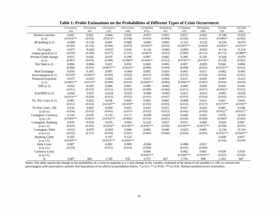
28

Table 1: Probit Estimations on the Probabilities of Different Types of Crisis Occurrences (1) Currency (2) Currency (3) Currency (4) Currency (5) Banking (6) Banking (7) Banking (8) Banking (9) Debt (10) Debt

Full IDC LDC EMG FULL IDC LDC EMG LDC EMG

Relative income 0.041 0.051 0.064 0.026 -0.017 0.001 0.012 0.026 -0.108 -0.023 (t-1) (0.015)*** (0.035) (0.027)** (0.040) (0.014) (0.004) (0.026) (0.037) (0.049)** (0.026)

IR holding (t-1) -0.004 -0.156 0.001 0.008 -0.093 0.003 -0.131 -0.122 -0.124 -0.079 (0.041) (0.135) (0.044) (0.075) (0.041)** (0.016) (0.047)*** (0.064)* (0.050)** (0.031)**

Per Capita -0.071 -0.243 -0.032 0.016 -0.124 -0.063 -0.063 -0.032 -0.134 -0.214 Output growth (t-1) (0.078) (0.206) (0.077) (0.161) (0.067)* (0.053) (0.069) (0.115) (0.113) (0.088)**

Private Credit change 0.015 0.056 0.035 0.190 0.097 0.002 0.209 0.150 -0.104 -0.070 (t-1) (0.067) (0.079) (0.088) (0.096)** (0.045)** (0.012) (0.070)*** (0.076)** (0.128) (0.065)

Net Debt (t-1) 0.006 -0.004 0.021 0.052 0.008 0.005 0.007 -0.002 0.046 0.006 (0.006) (0.015) (0.007)*** (0.023)** (0.006) (0.004) (0.008) (0.016) (0.015)*** (0.012)

Real Exchange 0.019 0.105 0.007 -0.004 0.005 0.010 0.003 0.011 -0.002 -0.001 Overvaluation (t-1) (0.010)* (0.041)** (0.009) (0.020) (0.013) (0.008) (0.015) (0.020) (0.014) (0.011)

Financial Exposure -0.017 -0.023 -0.002 -0.025 0.013 0.004 0.015 0.010 -0.007 -0.012 (t-1) (0.006)*** (0.011)** (0.009) (0.019) (0.004)*** (0.004) (0.006)*** (0.007) (0.016) (0.014)

ERS (t-1) -0.012 -0.025 0.006 0.001 0.009 -0.002 0.009 0.020 0.035 0.016 (0.011) (0.019) (0.012) (0.018) (0.009) (0.004) (0.011) (0.017) (0.016)** (0.012)

KAOPEN (t-1) -0.042 -0.027 -0.024 -0.023 -0.009 -0.003 -0.011 -0.015 -0.001 -0.016 (0.015)*** (0.024) (0.015) (0.021) (0.012) (0.007) (0.013) (0.018) (0.016) (0.011)

Tri. Pol. Conv (t-1) 0.001 -0.022 0.036 0.043 0.005 0.002 -0.000 0.011 0.051 0.024 (0.011) (0.014) (0.014)*** (0.019)** (0.010) (0.003) (0.013) (0.017) (0.017)*** (0.010)**

Tri-Pol. Conv., SD 0.035 -0.001 0.039 0.052 0.045 0.012 0.027 0.024 0.081 0.038 (t-5|t-1) (0.036) (0.053) (0.041) (0.057) (0.033) (0.012) (0.042) (0.056) (0.053)13% (0.025)11%

Contagion: Currency 0.143 0.078 0.135 0.117 -0.050 -0.024 -0.042 0.025 0.076 -0.019 (t or t-1) (0.030)*** (0.047)* (0.031)*** (0.066)* (0.035) (0.021) (0.036) (0.049) (0.040)* (0.045)

Contagion: Banking 0.035 -0.034 0.055 0.093 0.124 0.027 0.073 0.089 -0.022 0.007 (t or t-1) (0.025) (0.036) (0.024)** (0.034)*** (0.018)*** (0.026) (0.019)*** (0.027)*** (0.038) (0.025)

Contagion: Debt -0.015 -0.075 -0.003 0.046 0.005 0.046 -0.023 0.005 -0.234 -0.129 (t or t-1) (0.032) (0.127) (0.034) (0.061) (0.043) (0.044) (0.034) (0.056) (0.053)*** (0.034)***

Banking Crisis 0.102 0.107 0.124 0.030 0.027 (t or t-1) (0.029)*** (0.032)*** (0.044)*** (0.024) (0.019)

Debt Crisis 0.007 0.001 0.009 -0.004 -0.006 0.011 (t or t-1) (0.014) (0.012) (0.024) (0.009) (0.010) (0.020)

Currency Crisis 0.056 0.092 0.091 0.030 0.019 (t or t-1) (0.020)*** (0.028)*** (0.033)*** (0.023) (0.016)

N 2,407 662 1,745 932 2,372 627 1,745 906 1,562 847 Notes: The table reports the change in the probability of a crisis in response to a 1 unit change in the variable evaluated at the mean of all variables (x 100, to convert into percentages) with associated z-statistic (for hypothesis of no effect) in parentheses below. * p<0.1; ** p<0.05; *** p<0.01. Robust standard errors in brackets.

29

Table 2: Output Cost of Different Types of Crises Currency Currency Currency Banking Banking Banking Debt Debt FULL LDC EMG FULL LDC EMG LDC EMG (1) (2) (3) (4) (5) (6) (7) (8)

Relative income 0.003 0.818 1.371 0.064 0.673 1.299 1.931 -0.173 (t0-1) (0.167) (0.393)** (0.609)** (0.193) (0.431) (0.562)** (0.435)*** (1.151)

IR holding(t0-1) -0.259 -0.388 -0.453 -0.584 -0.690 0.579 -0.477 -1.837 (0.232) (0.334) (0.576) (0.576) (0.793) (0.999) (0.679) (1.080)

Per capita GDP -3.340 -3.521 -0.456 -5.717 -6.004 -3.637 -2.779 -4.159 Growth (t0-1) (1.123)*** (1.022)*** (1.445) (1.211)*** (1.313)*** (2.174) (0.854)*** (1.887)**

Private Credit change 1.007 1.503 0.756 0.688 0.701 4.961 -0.612 -2.246 (t0-1) (0.753) (0.907) (1.641) (1.026) (2.521) (2.801)* (0.994) (1.278)*

Exch. Overval.(t0-1) 0.702 0.729 0.518 -0.057 -0.060 0.286 0.231 0.215 (0.154)*** (0.195)*** (0.262)* (0.098) (0.126) (0.246) (0.104)** (0.246)

Net Debt(t0-1) -0.025 0.151 1.071 -0.059 -0.213 0.564 0.204 0.313 (0.158) (0.193) (0.403)** (0.101) (0.208) (0.300)* (0.144) (0.435)

Financial exposure 0.057 0.049 0.266 0.074 0.322 0.778 -0.083 -0.036 (t0-1) (0.157) (0.161) (0.367) (0.033)** (0.276) (0.595) (0.141) (0.312)

Deposit Insurance -0.105 -0.116 -0.128 -0.282 -0.379 -0.269 -0.169 0.092 (t0-1) (0.073) (0.093) (0.130) (0.102)*** (0.134)*** (0.231) (0.099)* (0.134)

ERS (t0-1) -0.254 -0.244 -0.289 -0.126 -0.161 -0.613 -0.097 -0.002 (0.132)* (0.173) (0.238) (0.159) (0.208) (0.353) (0.141) (0.325)

KAOPEN (t0-1) 0.133 0.142 0.516 0.214 0.217 0.324 0.080 0.332 (0.123) (0.123) (0.190)** (0.151) (0.197) (0.351) (0.205) (0.273)

Tri.Pol.Conv, d(t0-1) -0.199 -0.279 -0.553 -0.176 -0.281 -0.334 -0.049 0.118 (0.100)* (0.142)* (0.198)*** (0.121) (0.195) (0.277) (0.128) (0.296)

Tri-Pol. Conv., SD 0.160 0.097 0.445 -0.217 -0.773 -1.322 -0.138 -0.690 (t-5|t-1) (0.339) (0.402) (0.613) (0.337) (0.605) (0.966) (0.446) (0.866)

Banking Crisis 0.215 0.229 0.022 0.205 0.049 (t0-1, t0, or t0+1) (0.090)** (0.102)** (0.147) (0.140) (0.223)

Debt Crisis 0.118 0.023 0.172 0.099 0.083 0.265 (t0-1, t0, or t0+1) (0.126) (0.131) (0.154) (0.130) (0.159) (0.178) Currency Crisis 0.252 0.252 -0.184 0.116 0.170 (t0-1, t0, or t0+1) (0.100)** (0.121)** (0.190) (0.132) (0.240)

Adjusted R2 0.47 0.53 0.37 0.28 0.27 0.40 0.40 0.22 N 126 95 56 92 69 36 130 41

Notes: Robust standard errors in brackets. The dummy for the debt crisis of 1982 and the Asian financial crisis of 1997-98, and the global financial crisis of 2008-10 are also included, but not reported. The estimates for the constant term are also omitted. The terms of trade shocks variable is removed from the currency crisis output loss estimations since it is persistently statistically insignificant.

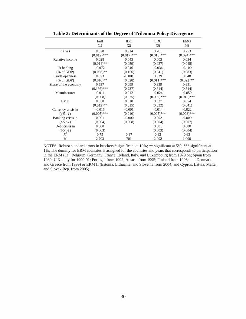
30

Table 3: Determinants of the Degree of Trilemma Policy Divergence

Full IDC LDC EMG (1) (2) (3) (4)

d (t-1) 0.828 0.914 0.761 0.753 (0.012)*** (0.017)*** (0.016)*** (0.024)***

Relative income 0.028 0.043 0.003 0.034 (0.014)** (0.059) (0.027) (0.048)

IR hodling -0.072 0.046 -0.034 -0.100 (% of GDP) (0.036)** (0.156) (0.041) (0.083)

Trade openness 0.023 -0.001 0.029 0.048 (% of GDP) (0.010)** (0.028) (0.011)*** (0.022)**

Share of the economy 0.637 0.099 0.339 0.651 (0.195)*** (0.237) (0.614) (0.714)

Manufacturer -0.011 0.012 -0.024 -0.059 (0.008) (0.025) (0.009)*** (0.016)***

EMU 0.030 0.018 0.037 0.054 (0.012)** (0.015) (0.032) (0.041)

Currency crisis in -0.015 -0.001 -0.014 -0.022 (t-5|t-1) (0.005)*** (0.010) (0.005)*** (0.008)***

Banking crisis in 0.001 -0.000 0.002 -0.000 (t-5|t-1) (0.004) (0.008) (0.004) (0.007)

Debt crisis in 0.000 0.001 0.000 (t-5|t-1) (0.003) (0.003) (0.004)

R2 0.75 0.87 0.62 0.63 N 2,703 701 2,002 1,000

NOTES: Robust standard errors in brackets * significant at 10%; ** significant at 5%; *** significant at 1%. The dummy for ERM countries is assigned for the countries and years that corresponds to participation in the ERM (i.e., Belgium, Germany, France, Ireland, Italy, and Luxembourg from 1979 on; Spain from 1989; U.K. only for 1990-91; Portugal from 1992; Austria from 1995; Finland from 1996; and Denmark and Greece from 1999) or ERM II (Estonia, Lithuania, and Slovenia from 2004; and Cyprus, Latvia, Malta, and Slovak Rep. from 2005).

31

Table 4: Effects of Past Crises on the Degree of Trilemma Policy Divergence

Singular effect of Crisis

Full t-1 t-2 t-3 t-4 t-5 t-6 t-7 t-8 t-9 t-10

Currency -0.065 -0.038

Banking

Debt

Industrialized countries t-1 t-2 t-3 t-4 t-5 t-6 t-7 t-8 t-9 t-10

Currency 0.075

Banking -0.169

Debt -- -- -- -- -- -- -- -- -- --

Developing countries t-1 t-2 t-3 t-4 t-5 t-6 t-7 t-8 t-9 t-10

Currency -0.066

Banking

Debt

Emerging markets t-1 t-2 t-3 t-4 t-5 t-6 t-7 t-8 t-9 t-10

Currency -0.071

Banking -0.082

Debt -0.084

Twin Crises (‘Marginal’ Effects)

Full t-1 t-2 t-3 t-4 t-5 t-6 t-7 t-8 t-9 t-10

Currency & Banking -0.081

Currency & Debt -0.060

Banking & Debt 0.093

Industrialized countries t-1 t-2 t-3 t-4 t-5 t-6 t-7 t-8 t-9 t-10

Currency & Banking 0.384

-- -- -- -- -- -- -- -- -- -- --

-- -- -- -- -- -- -- -- -- -- --



Currency & Debt -0.066 0.103




Currency & Debt -0.106

Banking & Debt 0.135 0.193

Notes: The upper half of the table reports only the significant weighted autoregressive estimates for the crisis dummies based on estimation equation (4). It must be noted that the estimation model does not include the twin crisis dummies. The bottom half of the table displays significant autoregressive estimates only for the (weighted) twin crisis dummies. The estimates on the (weighted) twin crisis dummies should be regarded as the marginal effect of past twin crises because the estimation model controls for the (weighted) autoregressive crisis dummies (though the estimates are not reported). Because there is no debt crisis episode for the industrialized countries in the sample, the estimate of the debt crisis or the estimates of currency and debt or banking and debt twin crises are unavailable for the group of industrialized countries.

32

Table 5: Effects of Past Output Losses on the Degree of Trilemma Policy Divergence

Singular effect of Crisis

Full t-1 t-2 t-3 t-4 t-5 t-6 t-7 t-8 t-9 t-10

Currency -0.081 -0.044

Banking

Debt


Currency 0.039 -0.080 -0.080

Banking

Debt


Currency -0.072 -0.084 -0.119

Banking 0.125

Debt

Twin Crises (‘Marginal’ Effects)

Full t-1 t-2 t-3 t-4 t-5 t-6 t-7 t-8 t-9 t-10



Banking & Debt


Currency & Banking -0.076 -0.114 -0.111




Currency & Banking -0.118 -0.190 -0.217



Notes: The upper half of the table reports only the significant autoregressive estimates for the weighted dummies for crises with output losses. It must be noted that the estimation model does not include the dummies for twin crises with output losses. The bottom half of the table displays significant autoregressive estimates only for the dummies for twin crises with output losses. Because the estimation model controls for the (weighted) autoregressive dummies for the crises with output losses (though not reported), the estimates on the dummies for twin crises with output losses should be regarded as the marginal effect of past twin crises with output losses.

33

Figure 1: The Trilemma Triangle

Exchange Rate Stability Monetary Union / Currency Boarde.g. Euro, Gold Stand., Hong Kong

Financially closed system

e.g., Bretton Woods

Floating exchange rate regime

e.g., Japan, Canada

Figure 2: Degree of Policy Dispersions among Different Income Groups of Countries

.6.8

11.

21.

41.

6

1970 1980 1990 2000 2010Year

Non-Euro Adv. Econ Euro Econ. minus Germany

Non-EMG LDC Emerging Market Economies

Note: 'Euro economies' include Austria, Beligium, France, Italy, Netherlands,Finland, Greece, Ireland, Portugal, and Spain

34

Figure 3: Degree of Policy Dispersions among Different Regional Country Groups

.6.8

11.

21.

41.

6

1970 1980 1990 2000 2010Year

Emerging Asia Developing Asia

Latin America and Carribbeans Others

Note: 'Emerging Asia' include China, Hong Kong, Korea, Indonesia, Thailand,Malaysia, Philippines, and Singapore

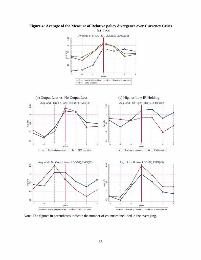
35

Figure 4: Average of the Measure of Relative policy divergence over Currency Crisis (a) Total

(b) Output Loss vs. No Output Loss (c) High or Low IR Holding

Note: The figures in parentheses indicate the number of countries included in the averaging.

.85

.9.9

51

1.05

Avg

. of d

-3 -2 -1 0 1 2 3years

Industrial countries Developing countries EMG countries

Average of d: IDC(43), LDC(159),EMG(75)

.85

.9.9

51

1.05

Avg

. of d

-3 -2 -1 0 1 2 3years

Developing countries EMG countries

Avg. of d - Output Loss: LDC(96),EMG(52).8

5.9

.95

11.

05A

vg. o

f d

-3 -2 -1 0 1 2 3years


Avg. of d - IR High: LDC(64),EMG(30)

.85

.9.9

51

1.05

Avg

. of d

-3 -2 -1 0 1 2 3years


Avg. of d - No Output Loss: LDC(57),EMG(22)

.85

.9.9

51

1.05

Avg

. of d

-3 -2 -1 0 1 2 3years


Avg. of d - IR Low: LDC(89),EMG(45)

36

Figure 5: Average of the Measure of Relative policy divergence over Banking Crisis (a) Total



.8.9

11.

11.

2A

vg.

of d

-3 -2 -1 0 1 2 3years


Average of d: IDC(23), LDC(98),EMG(44)

.7.7

5.8

.85

.9.9

51

1.05

Avg

. of d

-3 -2 -1 0 1 2 3years


Avg. of d - Output Loss: LDC(64),EMG(33)

.7.7

5.8

.85

.9.9

51

1.05

Avg

. of d

-3 -2 -1 0 1 2 3years



.7.7

5.8

.85

.9.9

51

1.05

Avg

. of d

-3 -2 -1 0 1 2 3years



.7.7

5.8

.85

.9.9

51

1.05

Avg

. of d

-3 -2 -1 0 1 2 3years



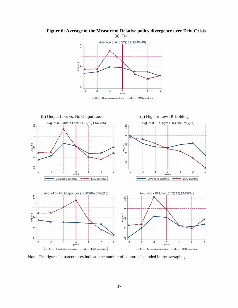
37

Figure 6: Average of the Measure of Relative policy divergence over Debt Crisis (a) Total



.85

.9.9

51

1.05

Avg

. of d

-3 -2 -1 0 1 2 3years


Average of d: LDC(189),EMG(48)

.85

.9.9

51

1.05

Avg

. of d

-3 -2 -1 0 1 2 3years


Avg. of d - Output Loss: LDC(89),EMG(35).8

5.9

.95

11.

05A

vg. o

f d

-3 -2 -1 0 1 2 3years



.85

.9.9

51

1.05

Avg

. of d

-3 -2 -1 0 1 2 3years



.85

.9.9

51

1.05

Avg

. of d

-3 -2 -1 0 1 2 3years



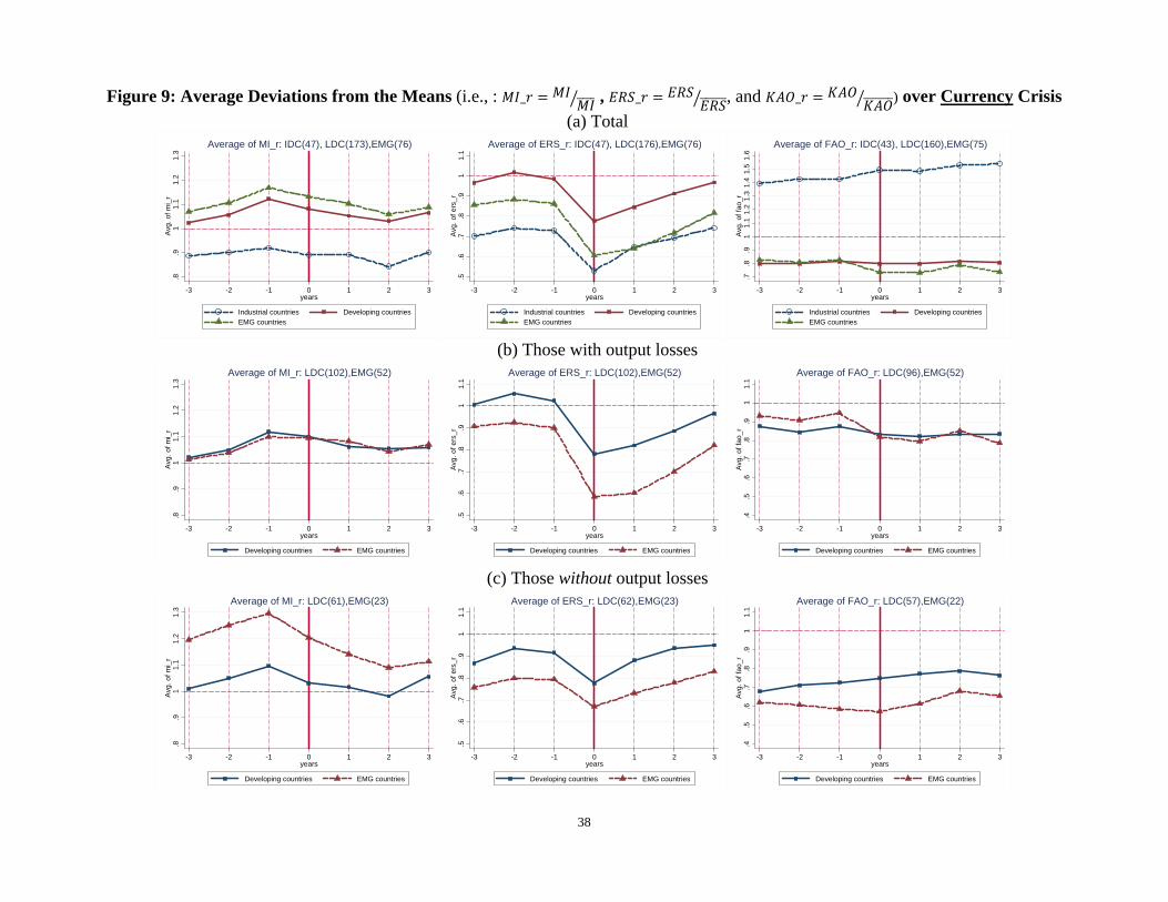
38

Figure 9: Average Deviations from the Means (i.e., : _ , _ , and _ ) over Currency Crisis

(a) Total

(b) Those with output losses

(c) Those without output losses

.8.9

11

.11

.21

.3A

vg.

of

mi_

r

-3 -2 -1 0 1 2 3years


Average of MI_r: IDC(47), LDC(173),EMG(76)

.5.6

.7.8

.91

1.1

Avg

. o

f e

rs_

r

-3 -2 -1 0 1 2 3years


Average of ERS_r: IDC(47), LDC(176),EMG(76)

.7.8

.91

1.1

1.2

1.3

1.4

1.5

1.6

Avg

. o

f fa

o_

r

-3 -2 -1 0 1 2 3years


Average of FAO_r: IDC(43), LDC(160),EMG(75)

.8.9

11

.11

.21

.3A

vg.

of

mi_

r

-3 -2 -1 0 1 2 3years


Average of MI_r: LDC(102),EMG(52)

.5.6

.7.8

.91

1.1

Avg

. o

f e

rs_

r

-3 -2 -1 0 1 2 3years


Average of ERS_r: LDC(102),EMG(52)

.4.5

.6.7

.8.9

11

.1A

vg.

of

fao

_r

-3 -2 -1 0 1 2 3years


Average of FAO_r: LDC(96),EMG(52)

.8.9

11

.11

.21

.3A

vg.

of

mi_

r

-3 -2 -1 0 1 2 3years



.5.6

.7.8

.91

1.1

Avg

. o

f e

rs_

r

-3 -2 -1 0 1 2 3years



.4.5

.6.7

.8.9

11

.1A

vg.

of

fao

_r

-3 -2 -1 0 1 2 3years



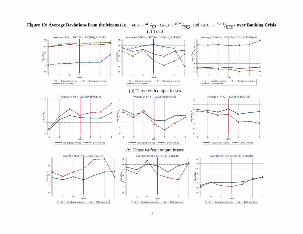
39

Figure 10: Average Deviations from the Means (i.e., : _ , _ , and _ ) over Banking Crisis

(a) Total

(b) Those with output losses

(c) Those without output losses

.2.4

.6.8

11

.2A

vg.

of

mi_

r

-3 -2 -1 0 1 2 3years


Average of MI_r: IDC(24), LDC(103),EMG(45)

.5.6

.7.8

.91

1.1

Avg

. o

f e

rs_

r

-3 -2 -1 0 1 2 3years


Average of ERS_r: IDC(24), LDC(114),EMG(48)

.6.8

11

.21

.41

.61

.82

Avg

. o

f fa

o_

r

-3 -2 -1 0 1 2 3years


Average of FAO_r: IDC(25), LDC(104),EMG(46)

.91

1.1

1.2

Avg

. o

f m

i_r

-3 -2 -1 0 1 2 3years



.5.6

.7.8

.91

1.1

Avg

. o

f e

rs_

r

-3 -2 -1 0 1 2 3years



.4.5

.6.7

.8.9

11

.1A

vg.

of

fao

_r

-3 -2 -1 0 1 2 3years



.91

1.1

1.2

Avg

. o

f m

i_r

-3 -2 -1 0 1 2 3years



.5.6

.7.8

.91

1.1

Avg

. o

f e

rs_

r

-3 -2 -1 0 1 2 3years



.4.5

.6.7

.8.9

11

.1A

vg.

of

fao

_r

-3 -2 -1 0 1 2 3years



40

Figure 11: Average of the Measure of Relative policy divergence for Latin America and Asia

Notes: “Latin America” includes: Argentina, Bolivia, Brazil, Chile, Columbia, Costa Rica, Ecuador, El Salvador, Honduras, Mexico, Peru, Uruguay, and Venezuela. “Asia” includes: Indonesia, Korea, Malaysia, the Philippines, and Thailand. For each of the Latin American countries, “Year 0” indicates the year when the crisis is the most severe among the years: 1981. 1982, and 1983, i.e., it varies among the countries. For the Asian countries, “Year 0” is 1997.

.4.5

.6.7

.8.9

11.

1A

vg. o

f d

-5 -4 -3 -2 -1 0 1 2 3 4 5years

Latin America Asia

Average of d: LAMERICA (12) and Asia (5)

41

Figure 12: Average Deviations from the Means (i.e., : _ , _ , and

_ ) for Latin America (a) and Asia (b)

Notes: “Latin America” includes: Argentina, Bolivia, Brazil, Chile, Columbia, Costa Rica, Ecuador, El Salvador, Honduras, Mexico, Peru, Uruguay, and Venezuela. “Asia” includes: Indonesia, Korea, Malaysia, the Philippines, and Thailand. For each of the Latin American countries, “Year 0” indicates the year when the crisis is the most severe among the years: 1981. 1982, and 1983, i.e., it varies among the countries. For the Asian countries, “Year 0” is 1997.

.2.4

.6.8

11.

21.

4A

vg. o

f d

-5 -4 -3 -2 -1 0 1 2 3 4 5years

Monetary Indep. Exch. R. Stab. Financial Op.

(a) Latin America.2

.4.6

.81

1.2

1.4

Avg

. of d

-5 -4 -3 -2 -1 0 1 2 3 4 5years

Monetary Indep. Exch. R. Stab. Financial Op.

(b) Asia

LIVING WITH THE TRILEMMA CONSTRAINT: …web.pdx.edu/~ito/w19448.pdfLiving with the Trilemma...

Documents

Transcript of LIVING WITH THE TRILEMMA CONSTRAINT: …web.pdx.edu/~ito/w19448.pdfLiving with the Trilemma...