Linear system theory: linearization
29
NATIONAL CHENG KUNG UNIVERSITY Department of Mechanical Engineering LINEAR SYSTEM HOMEWORK 3 Instructor: Prof. Szu – Chi Tien Student: Nguyen Van Thanh Student ID: P96007019 Department: Inst. of Manufacturin g & Information Systems Class: 1001- N154000 – Linear System October 26, 2011
-
Upload
thanh-nguyen -
Category
Documents
-
view
226 -
download
0
Transcript of Linear system theory: linearization
7/29/2019 Linear system theory: linearization
http://slidepdf.com/reader/full/linear-system-theory-linearization 1/29
NATIONAL CHENG KUNG UNIVERSITY
Department of Mechanical Engineering
LINEAR SYSTEM
HOMEWORK 3
Instructor: Prof. Szu – Chi Tien
Student: Nguyen Van Thanh
Student ID: P96007019
Department: Inst. of Manufacturing & Information Systems
Class: 1001- N154000 – Linear System
October 26, 2011

7/29/2019 Linear system theory: linearization
http://slidepdf.com/reader/full/linear-system-theory-linearization 2/29
Linear System Theory Page 1
Contents
Problem 1 ....................................................................................................................... 2
Problem 2 ..................................................................................................................... 10 Problem 3 ..................................................................................................................... 19 Appendix A Matlab code for Problem 1 Part 4 ........................................................... 24 Appendix B Matlab code for Problem 1 Part 5 ........................................................... 25 Appendix C Matlab code for Problem 2 Part 2 ........................................................... 26 Appendix D Matlab code for Problem 2 Part 3 ........................................................... 27 Appendix E Matlab code for Problem 2 Part 4 ........................................................... 28
7/29/2019 Linear system theory: linearization
http://slidepdf.com/reader/full/linear-system-theory-linearization 3/29
Linear System Theory Page 2
Problem 1
Consider the nonlinear state equations (which were studied extensively in class)
1. Find A and B of the linearized state equations evaluated at the above given nominal
condition, where
Is the system stable?
Solution
Rewrite the nonlinear state equations
Solve
To find equilibrium states. Take one equilibrium state with
, -

7/29/2019 Linear system theory: linearization
http://slidepdf.com/reader/full/linear-system-theory-linearization 4/29
Linear System Theory Page 3
We can write as form
Where,
[
]
0 1
01 0 1 01
The polynomial characteristic equation of matrix A
The real part of the eigenvalues of matrix A are zero. Hence, the system is marginally
stable.
E.g. 0
1 , see Fig. 1.1.

7/29/2019 Linear system theory: linearization
http://slidepdf.com/reader/full/linear-system-theory-linearization 5/29
Linear System Theory Page 4
Figure 1.1 Perturbed state responses.
Solution
0 1
Solution for that system differential equations is
* + 0 1} 0 1

7/29/2019 Linear system theory: linearization
http://slidepdf.com/reader/full/linear-system-theory-linearization 6/29
Linear System Theory Page 5
01 The perturbed state responses are shown in Fig. 1.2.
Figure 1.2 Perturbed state responses with , -
Solution
7/29/2019 Linear system theory: linearization
http://slidepdf.com/reader/full/linear-system-theory-linearization 7/29
Linear System Theory Page 6
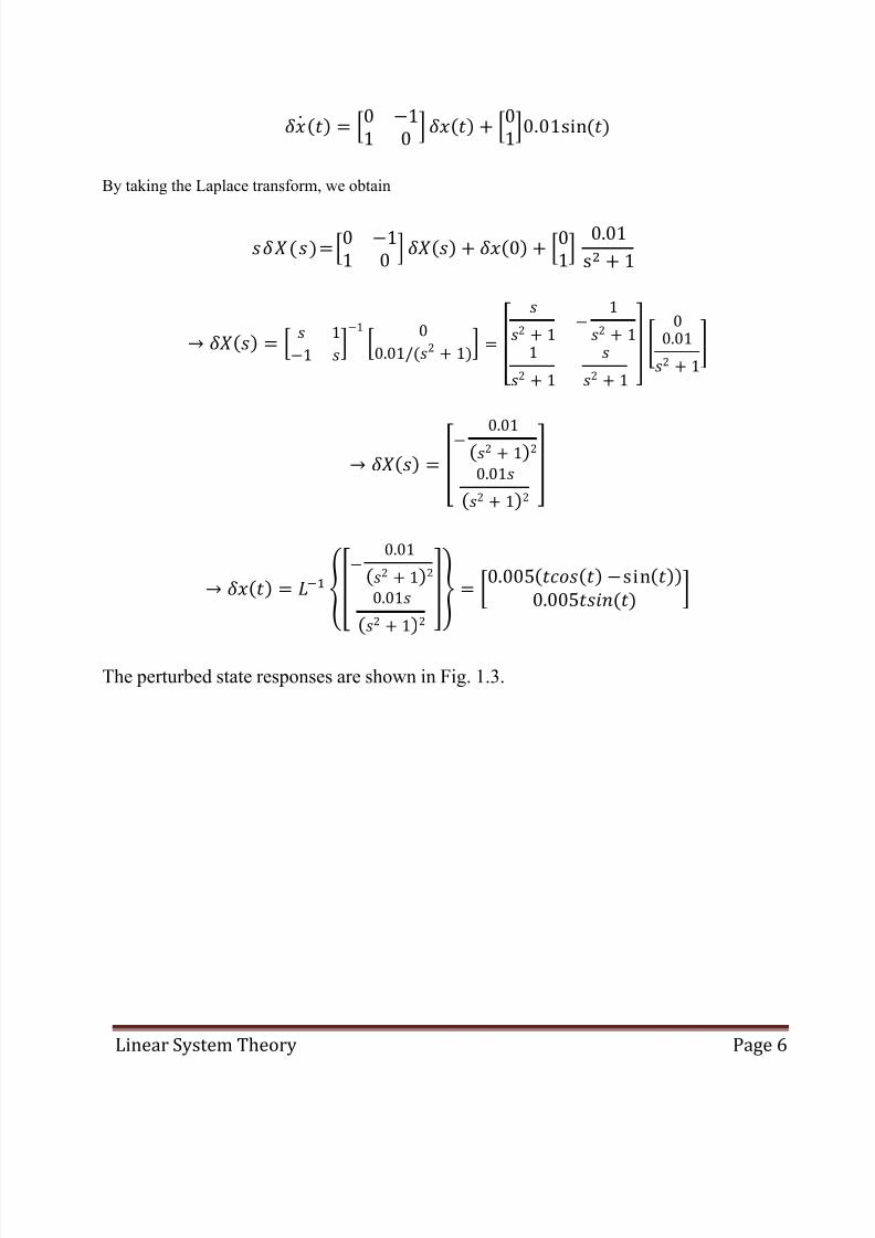
0 1 01
By taking the Laplace transform, we obtain
0 1 01 0 1 0 1
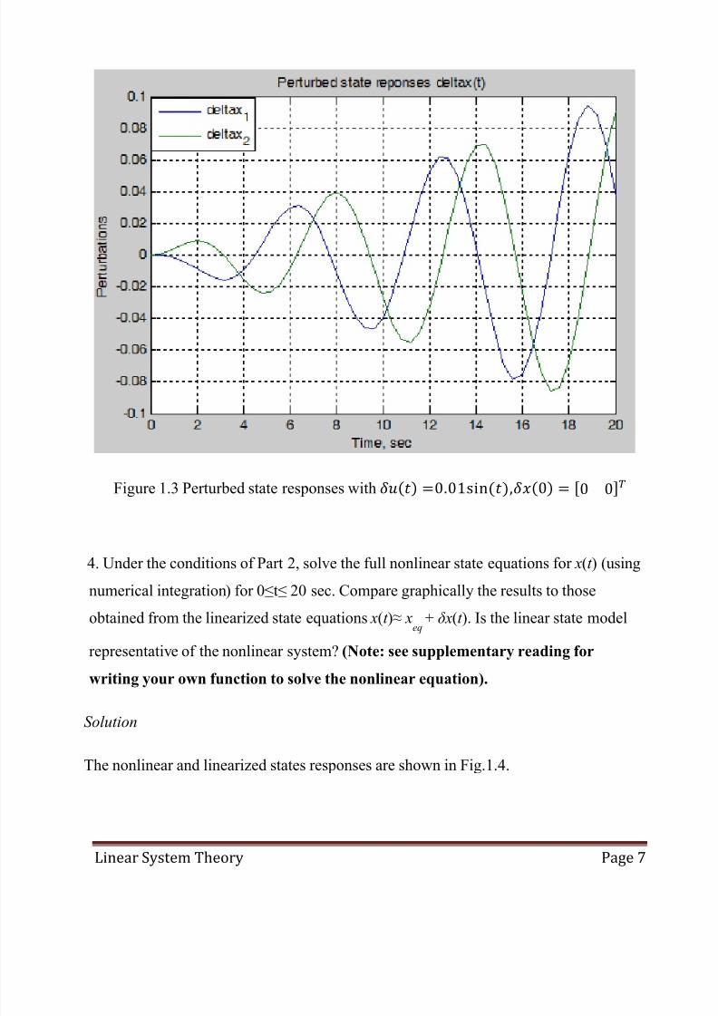
The perturbed state responses are shown in Fig. 1.3.
7/29/2019 Linear system theory: linearization
http://slidepdf.com/reader/full/linear-system-theory-linearization 8/29
Linear System Theory Page 7
Figure 1.3 Perturbed state responses with
, -
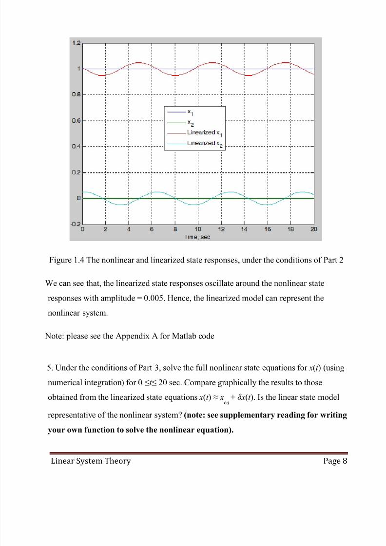
4. Under the conditions of Part 2, solve the full nonlinear state equations for x(t ) (using
numerical integration) for 0≤t≤ 20 sec. Compare graphically the results to those
obtained from the linearized state equations x(t )≈ xeq
+ δx(t ). Is the linear state model
representative of the nonlinear system? (Note: see supplementary reading for
writing your own function to solve the nonlinear equation).
Solution
The nonlinear and linearized states responses are shown in Fig.1.4.
7/29/2019 Linear system theory: linearization
http://slidepdf.com/reader/full/linear-system-theory-linearization 9/29
Linear System Theory Page 8
Figure 1.4 The nonlinear and linearized state responses, under the conditions of Part 2
We can see that, the linearized state responses oscillate around the nonlinear state
responses with amplitude = 0.005. Hence, the linearized model can represent the
nonlinear system.
Note: please see the Appendix A for Matlab code
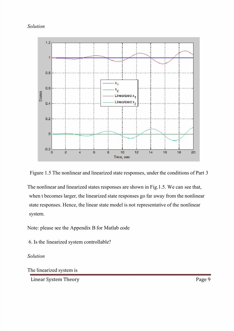
5. Under the conditions of Part 3, solve the full nonlinear state equations for x(t ) (using
numerical integration) for 0 ≤t ≤ 20 sec. Compare graphically the results to those
obtained from the linearized state equations x(t ) ≈ xeq
+ δx(t ). Is the linear state model
representative of the nonlinear system? (note: see supplementary reading for writing
your own function to solve the nonlinear equation).
7/29/2019 Linear system theory: linearization
http://slidepdf.com/reader/full/linear-system-theory-linearization 10/29
Linear System Theory Page 9
Solution
Figure 1.5 The nonlinear and linearized state responses, under the conditions of Part 3
The nonlinear and linearized states responses are shown in Fig.1.5. We can see that,
when t becomes larger, the linearized state responses go far away from the nonlinear
state responses. Hence, the linear state model is not representative of the nonlinear
system.
Note: please see the Appendix B for Matlab code
6. Is the linearized system controllable?
Solution
The linearized system is

7/29/2019 Linear system theory: linearization
http://slidepdf.com/reader/full/linear-system-theory-linearization 11/29
Linear System Theory Page 10
0 1 01
We will use the controllability matrix to test the system is controllable or not.
Controllability matrix
, - 0 1
Controllability matrix C has full rank. Hence, the system is controllable.
Problem 2
Given the following linear time-invariant system
I will use Matlab to solve this problem.
1. Is the system controllable? Explain.
Solution
The controllability matrix
, - 0 1
The controllability matrix C has full rank. Hence, the system is controllable.
7/29/2019 Linear system theory: linearization
http://slidepdf.com/reader/full/linear-system-theory-linearization 12/29
Linear System Theory Page 11
2. Find a control input u(t) that bring the system states to () , -, where, . Confirm your results with simulation of the responses for 0 ≤ t
≤ 15 sec.
Solution
From Par1, the system is controllable, thus the controllability Grammian matrix is
invertible. The controllability Grammian matrix
Given x(0) and x(tf ), we choose a control input u(t)
, -
(
) . (
)/
( ) ( ) 0 1
( ) ∫
7/29/2019 Linear system theory: linearization
http://slidepdf.com/reader/full/linear-system-theory-linearization 13/29
Linear System Theory Page 12
We can find the response through
7/29/2019 Linear system theory: linearization
http://slidepdf.com/reader/full/linear-system-theory-linearization 14/29
Linear System Theory Page 13
( ) ∫
7/29/2019 Linear system theory: linearization
http://slidepdf.com/reader/full/linear-system-theory-linearization 15/29
Linear System Theory Page 14
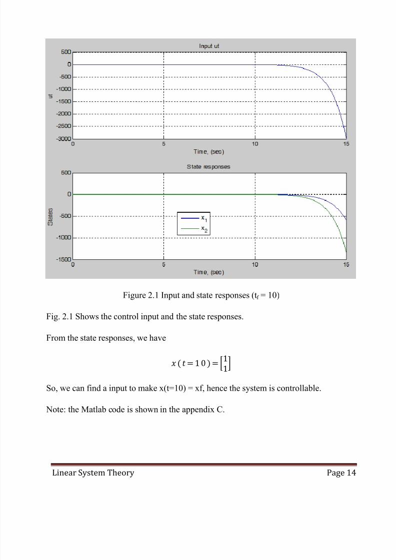
Figure 2.1 Input and state responses (tf = 10)
Fig. 2.1 Shows the control input and the state responses.
From the state responses, we have
0
1 So, we can find a input to make x(t=10) = xf, hence the system is controllable.
Note: the Matlab code is shown in the appendix C.
7/29/2019 Linear system theory: linearization
http://slidepdf.com/reader/full/linear-system-theory-linearization 16/29
Linear System Theory Page 15
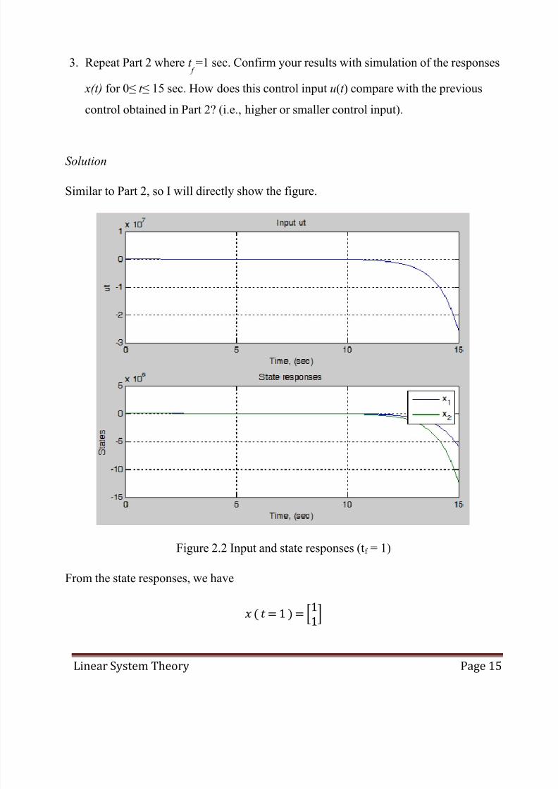
3. Repeat Part 2 where t f
=1 sec. Confirm your results with simulation of the responses
x(t) for 0≤ t ≤ 15 sec. How does this control input u(t ) compare with the previous
control obtained in Part 2? (i.e., higher or smaller control input).
Solution
Similar to Part 2, so I will directly show the figure.
Figure 2.2 Input and state responses (tf = 1)
From the state responses, we have
01

7/29/2019 Linear system theory: linearization
http://slidepdf.com/reader/full/linear-system-theory-linearization 17/29
Linear System Theory Page 16
So, we can find a input to make x(t = 1) = xf , hence the system is controllable. And, we
can see that we need higher control input compare to Part 2 to control system. Hence, if
a system is controllable, we want to bring this to a given tf in a shorter time, we need
more input.
Note: the Matlab code is shown in the appendix D.
4. Find a totally different solution to the control input u(t ) that solves Part 2. That is,
the solution u(t )in Part 2 is NOT unique. For example, in digital control let
Where u1, u
2and t
1are constant parameters (to be determined) that provide another
control input u(t ) for the solution of Part 2.
Solution
If we can find a different input
to control the system as we want, and u1, u2, t1 are all constants, then the solution (or
responses) x(t) can be represented as
() . ( )/ ∫ . ( )/
∫ . ( )/
7/29/2019 Linear system theory: linearization
http://slidepdf.com/reader/full/linear-system-theory-linearization 18/29
Linear System Theory Page 17
01 ∫ . ( )/
∫ . ( )/
() . ( )/
01
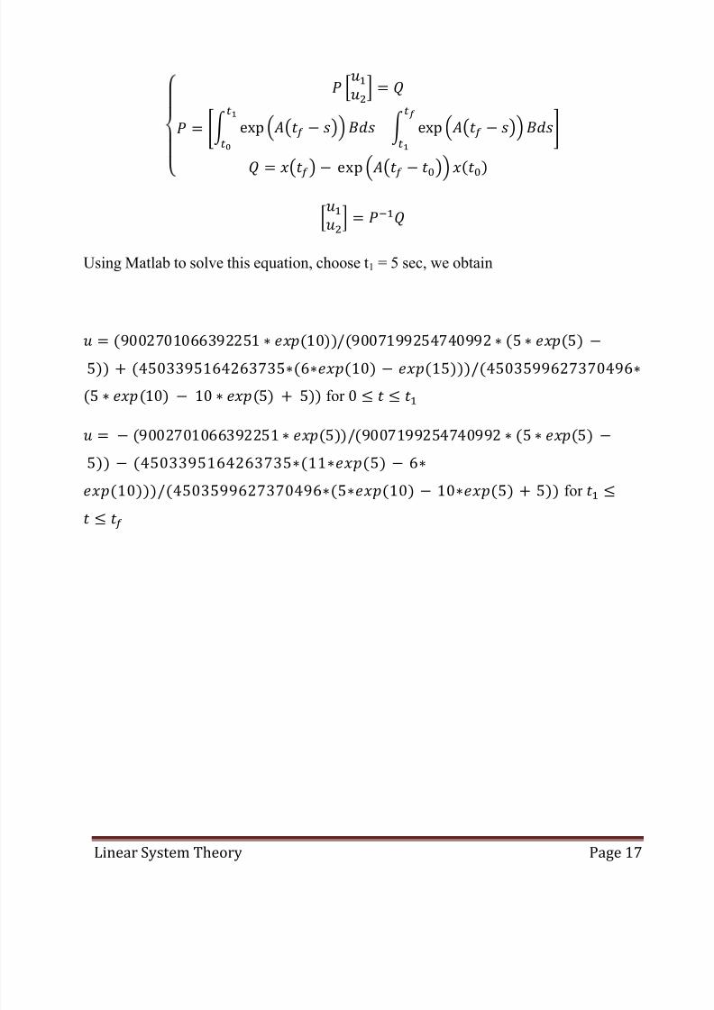
Using Matlab to solve this equation, choose t1 = 5 sec, we obtain
for
for

7/29/2019 Linear system theory: linearization
http://slidepdf.com/reader/full/linear-system-theory-linearization 19/29
Linear System Theory Page 18
Figure 2.3 Input and state responses
A control input
for all , - and bring this system from initial sates to
final states, since x(t = tf = 10) = xf .
Note: the Matlab code is shown in the appendix E.

7/29/2019 Linear system theory: linearization
http://slidepdf.com/reader/full/linear-system-theory-linearization 20/29
Linear System Theory Page 19
Problem 3
Consider the following linear time-invariant system,
1. Is the system controllable? Explain.
Solution
The controllability matrix
, -
Hence, the controllability Grammian is not invertible, so the system is uncontrollable.
2. Is the system stabilizable? Explain.
The characteristic polynomial equation of matrix A
There exists one that is positive, the system thus is unstable.
3. Identify the modes that are uncontrollable.
We will use the PHB rank test
, -
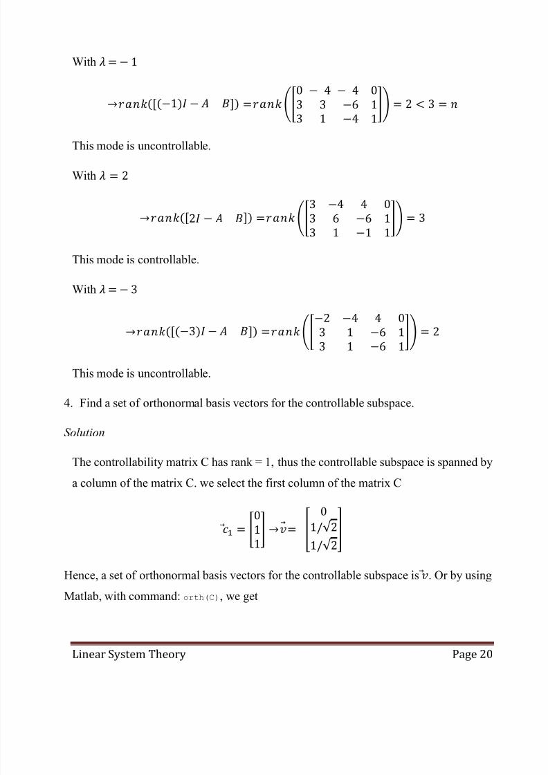
7/29/2019 Linear system theory: linearization
http://slidepdf.com/reader/full/linear-system-theory-linearization 21/29
Linear System Theory Page 20
With
, -
This mode is uncontrollable.
With
, -
This mode is controllable.
With
, -
This mode is uncontrollable.
4. Find a set of orthonormal basis vectors for the controllable subspace.
Solution
The controllability matrix C has rank = 1, thus the controllable subspace is spanned by
a column of the matrix C. we select the first column of the matrix C
√ √
Hence, a set of orthonormal basis vectors for the controllable subspace is . Or by using
Matlab, with command: orth(C), we get

7/29/2019 Linear system theory: linearization
http://slidepdf.com/reader/full/linear-system-theory-linearization 22/29
Linear System Theory Page 21
5.
Find a set of basis vectors for the uncontrollable subspace. Are there vectorsorthogonal to the controllable subspace?
Solution
From Part 4, the uncontrollable subspace must be of dimension . We can choose any two linearity independent vectors that are
not in the controllable subspace, for example
√ √√
So, a set of basis vectors for the uncontrollable subspace is √ √ √
We can check
These two vectors are orthogonal to the controllable subspace. But, it is not necessary.
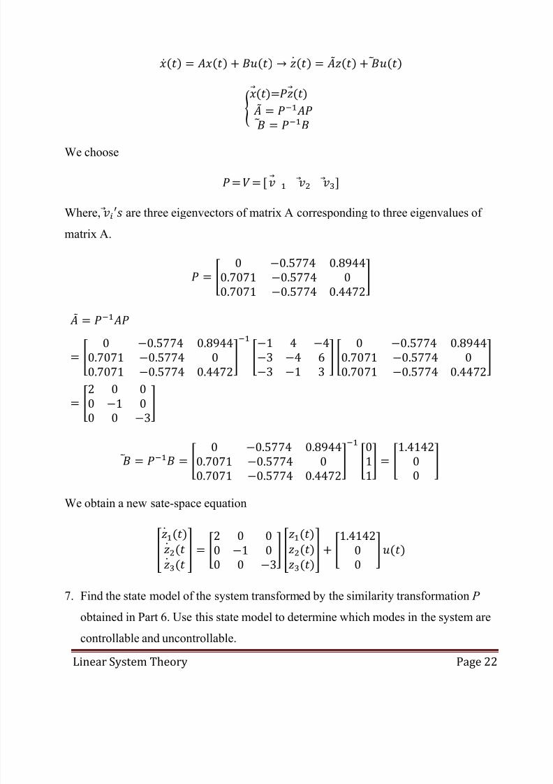
6. Determine a state transformation P that separates the system into controllable and
uncontrollable subspace, where Solution
From state transformation formula
7/29/2019 Linear system theory: linearization
http://slidepdf.com/reader/full/linear-system-theory-linearization 23/29
Linear System Theory Page 22
We choose
, - Where, are three eigenvectors of matrix A corresponding to three eigenvalues of
matrix A.
We obtain a new sate-space equation
7. Find the state model of the system transformed by the similarity transformation P
obtained in Part 6. Use this state model to determine which modes in the system are
controllable and uncontrollable.
7/29/2019 Linear system theory: linearization
http://slidepdf.com/reader/full/linear-system-theory-linearization 24/29
Linear System Theory Page 23
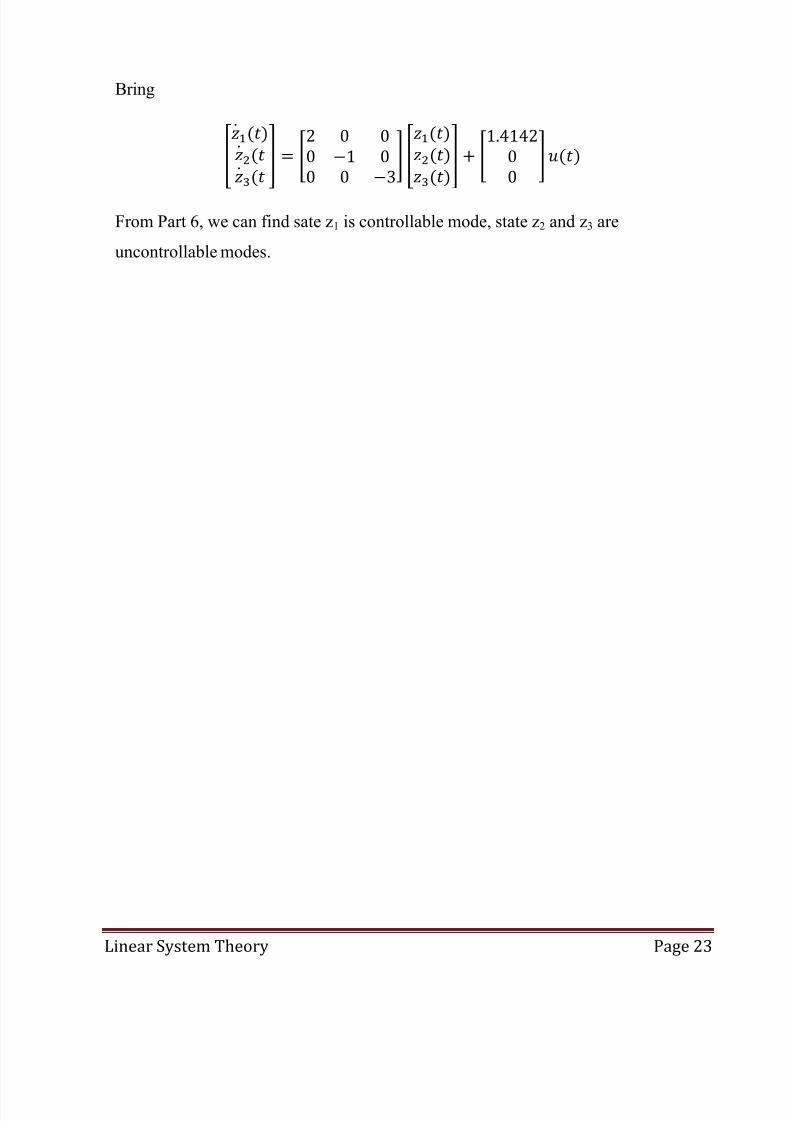
Bring
From Part 6, we can find sate z1 is controllable mode, state z2 and z3 are
uncontrollable modes.
7/29/2019 Linear system theory: linearization
http://slidepdf.com/reader/full/linear-system-theory-linearization 25/29
Linear System Theory Page 24
Appendix A Matlab code for Problem 1 Part 4
ODE function for the nonlinear system
function dx = xdiff(t,x) % nonlinear system u = 0; dx = zeros(2,1); dx(1) = x(2) - 2*x(1)*x(2); dx(2) = -x(1) + x(1)^2 + x(2)^2 + u; end
ODE function for perturbation
function ddx = dxdiff(dt,dx) % delta_x_diff = A*delta_x + B*delta_u; du = 0; ddx = zeros(2,1); ddx(1) = -dx(2); ddx(2) = dx(1) + du; end
m-file code
clc; clear all; close all; to = 0; tspan = 0.1; tfinal = 20; n = (tfinal - to)/tspan + 1;
% non-linear system xq = [1; 0]; [t,x] = ode45(@xdiff,to:tspan:tfinal,xq);
% perturbation dx0 = [0.01; 0.05]; [dt,dx] = ode45(@dxdiff,to:tspan:tfinal,dx0);
% linearized system x_linearized = zeros(n,2); x_linearized(:,1) = dx(:,1) + xq(1); x_linearized(:,2) = dx(:,2) + xq(2);
plot(t,x,dt,x_linearized); grid on; xlabel('Time, sec');
ylabel('States'); legend('x_1','x_2','Linearized x_1','Linearized x_2');

7/29/2019 Linear system theory: linearization
http://slidepdf.com/reader/full/linear-system-theory-linearization 26/29
Linear System Theory Page 25
Appendix B Matlab code for Problem 1 Part 5
function dx = xdiff(t,x) % nonlinear system u = 0; dx = zeros(2,1); dx(1) = x(2) - 2*x(1)*x(2); dx(2) = -x(1) + x(1)^2 + x(2)^2 + u; end
ODE function for perturbation
function ddx = dxdiff(dt,dx) % delta_x_diff = A*delta_x + B*delta_u; du = 0.01*sin(dt); ddx = zeros(2,1); ddx(1) = -dx(2); ddx(2) = dx(1) + du; end
m-file code
clc; clear all; close all; to = 0; tspan = 0.1; tfinal = 20; n = (tfinal - to)/tspan + 1;
% non-linear system xq = [1; 0]; [t,x] = ode45(@xdiff,to:tspan:tfinal,xq);
% perturbation dx0 = [0; 0]; [dt,dx] = ode45(@dxdiff,to:tspan:tfinal,dx0);
% linearized system x_linearized = zeros(n,2); x_linearized(:,1) = dx(:,1) + xq(1); x_linearized(:,2) = dx(:,2) + xq(2);
plot(t,x,dt,x_linearized); grid on; xlabel('Time, sec'); ylabel('States');
legend('x_1','x_2','Linearized x_1','Linearized x_2');

7/29/2019 Linear system theory: linearization
http://slidepdf.com/reader/full/linear-system-theory-linearization 27/29
Linear System Theory Page 26
Appendix C Matlab code for Problem 2 Part 2
close all; clear all; clc;
A = [-1 1; 0 -1]; B = [0;1]; x0 = [1; 1];
xf = [1; 1]; t0 = 0; tf = 10; syms t t1 s; Phitft = expm(A*(tf - t)); Phitft0 = expm(A*(tf - t0)); W = int(expm(A*s)*(B*B')*expm(A'*s),t0,tf - t0); u = B'*Phitft'*W^(-1)*(xf - Phitft0*x0); xt = expm(A*(t1 - t0))*x0 + int(expm(A*(t1 - t))*B*u,t0,t1);
t1 = 0:0.01:15; t = 0:0.01:15; ut = subs(u); x1 = subs(xt(1)); x2 = subs(xt(2));
subplot(211); plot(t,ut); title('Input ut'); xlabel('Time, (sec)'); ylabel('ut'); grid on; subplot(212); plot(t1,x1,t1,x2); title('State responses'); xlabel('Time, (sec)'); ylabel('States'); grid on; legend('x_1','x_2');

7/29/2019 Linear system theory: linearization
http://slidepdf.com/reader/full/linear-system-theory-linearization 28/29
Linear System Theory Page 27
Appendix D Matlab code for Problem 2 Part 3
close all; clear all; clc;
A = [-1 1; 0 -1]; B = [0;1]; x0 = [1; 1];
xf = [1; 1]; t0 = 0; tf = 1; syms t t1 s; Phitft = expm(A*(tf - t)); Phitft0 = expm(A*(tf - t0)); W = int(expm(A*s)*(B*B')*expm(A'*s),t0,tf - t0); u = B'*Phitft'*W^(-1)*(xf - Phitft0*x0); xt = expm(A*(t1 - t0))*x0 + int(expm(A*(t1 - t))*B*u,t0,t1);
t1 = 0:0.01:15; t = 0:0.01:15; ut = subs(u); x1 = subs(xt(1)); x2 = subs(xt(2));
subplot(211); plot(t,ut); title('Input ut'); xlabel('Time, (sec)'); ylabel('ut'); grid on; subplot(212); plot(t1,x1,t1,x2); title('State responses'); xlabel('Time, (sec)'); ylabel('States'); grid on; legend('x_1','x_2');

7/29/2019 Linear system theory: linearization
http://slidepdf.com/reader/full/linear-system-theory-linearization 29/29
Appendix E Matlab code for Problem 2 Part 4
close all; clear all; clc;
A = [-1 1; 0 -1];B = [0;1];
x0 = [1; 1]; xf = [1; 1]; t0 = 0; t1 = 5; tf = 10; syms t s; P1 = int(expm(A*(tf-s))*B,s,t0,t1); P2 = int(expm(A*(tf-s))*B,s,t1,tf); P = [P1 P2]; Q = xf - expm(A*(tf - t0))*x0; u = P^(-1)*Q; xt1 = expm(A*t)*x0 + int(expm(A*(t-s))*B*u(1),s,t0,t); % t = t0 ~ t1 xt2 = expm(A*t)*x0 + int(expm(A*(t-s))*B*u(1),s,t0,t1) + ...
int(expm(A*(t-s))*B*u(2),s,t1,t); %t = t1 ~ tf t = t0:0.01:t1; xt1 = subs(xt1); t = (t1 + 0.01):0.01:tf; xt2 = subs(xt2); xt11 = [xt1(1,:) xt2(1,:)]; xt22 = [xt1(2,:) xt2(2,:)]; t = t0:0.01:tf; u1 = subs(u(1)*ones(1,501)); u2 = subs(u(2)*ones(1,500)); subplot(211); plot(t(1:501),u1,t(502:1001),u2); title('Input ut'); xlabel('Time, (sec)'); ylabel('ut'); grid on; subplot(212); plot(t,xt11,t,xt22); title('State responses');
xlabel('Time, (sec)'); ylabel('States'); grid on; legend('x_1','x_2');


![LINEARIZATION - CaltechAUTHORS · The linear theory can also be developed on a separate footing, as in Gurtin [1972a]. Often, linearization of the equations of continuum mechanics](https://static.fdocuments.us/doc/165x107/5b446d8d7f8b9a56348b5245/linearization-caltechauthors-the-linear-theory-can-also-be-developed-on-a.jpg)