Linear Regression and Correlation - · PDF fileLinear Regression and Correlation ... is there...

Chapter 12

Linear Regression and Correlation

12.1 Linear Regression and Correlation1

12.1.1 Student Learning Objectives

By the end of this chapter, the student should be able to:

• Discuss basic ideas of linear regression and correlation.• Create and interpret a line of best fit.• Calculate and interpret the correlation coefficient.• Calculate and interpret outliers.

12.1.2 Introduction

Professionals often want to know how two or more variables are related. For example, is there a relationshipbetween the grade on the second math exam a student takes and the grade on the final exam? If there is arelationship, what is it and how strong is the relationship?

In another example, your income may be determined by your education, your profession, your years ofexperience, and your ability. The amount you pay a repair person for labor is often determined by an initialamount plus an hourly fee. These are all examples in which regression can be used.

The type of data described in the examples is bivariate data - "bi" for two variables. In reality, statisticiansuse multivariate data, meaning many variables.

In this chapter, you will be studying the simplest form of regression, "linear regression" with one indepen-dent variable (x). This involves data that fits a line in two dimensions. You will also study correlation whichmeasures how strong the relationship is.

12.2 Linear Equations2

Linear regression for two variables is based on a linear equation with one independent variable. It has theform:

y = a + bx (12.1)

1This content is available online at <http://http://cnx.org/content/m17089/1.5/>.2This content is available online at <http://http://cnx.org/content/m17086/1.4/>.

511

512 CHAPTER 12. LINEAR REGRESSION AND CORRELATION

where a and b are constant numbers.

x is the independent variable, and y is the dependent variable. Typically, you choose a value to substitutefor the independent variable and then solve for the dependent variable.

Example 12.1The following examples are linear equations.

y = 3 + 2x (12.2)

y = −0.01 + 1.2x (12.3)

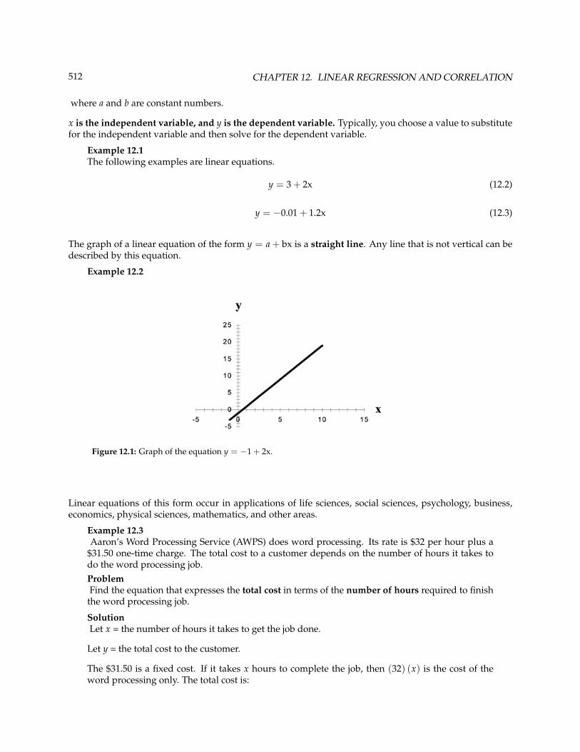
The graph of a linear equation of the form y = a + bx is a straight line. Any line that is not vertical can bedescribed by this equation.

Example 12.2

Figure 12.1: Graph of the equation y = −1 + 2x.

Linear equations of this form occur in applications of life sciences, social sciences, psychology, business,economics, physical sciences, mathematics, and other areas.

Example 12.3Aaron’s Word Processing Service (AWPS) does word processing. Its rate is $32 per hour plus a

$31.50 one-time charge. The total cost to a customer depends on the number of hours it takes todo the word processing job.ProblemFind the equation that expresses the total cost in terms of the number of hours required to finish

the word processing job.

SolutionLet x = the number of hours it takes to get the job done.

Let y = the total cost to the customer.

The $31.50 is a fixed cost. If it takes x hours to complete the job, then (32) (x) is the cost of theword processing only. The total cost is:

513

y = 31.50 + 32x

12.3 Slope and Y-Intercept of a Linear Equation3

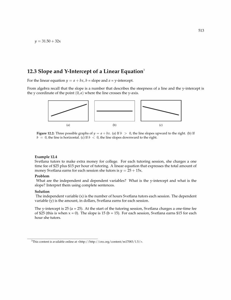
For the linear equation y = a + bx, b = slope and a = y-intercept.

From algebra recall that the slope is a number that describes the steepness of a line and the y-intercept isthe y coordinate of the point (0, a) where the line crosses the y-axis.

(a) (b) (c)

Figure 12.2: Three possible graphs of y = a + bx. (a) If b > 0, the line slopes upward to the right. (b) Ifb = 0, the line is horizontal. (c) If b < 0, the line slopes downward to the right.

Example 12.4Svetlana tutors to make extra money for college. For each tutoring session, she charges a onetime fee of $25 plus $15 per hour of tutoring. A linear equation that expresses the total amount ofmoney Svetlana earns for each session she tutors is y = 25 + 15x.ProblemWhat are the independent and dependent variables? What is the y-intercept and what is the

slope? Interpret them using complete sentences.

SolutionThe independent variable (x) is the number of hours Svetlana tutors each session. The dependentvariable (y) is the amount, in dollars, Svetlana earns for each session.

The y-intercept is 25 (a = 25). At the start of the tutoring session, Svetlana charges a one-time feeof $25 (this is when x = 0). The slope is 15 (b = 15). For each session, Svetlana earns $15 for eachhour she tutors.

3This content is available online at <http://http://cnx.org/content/m17083/1.5/>.


12.4 Scatter Plots4

Before we take up the discussion of linear regression and correlation, we need to examine a way to displaythe relation between two variables x and y. The most common and easiest way is a scatter plot. Thefollowing example illustrates a scatter plot.

Example 12.5From an article in the Wall Street Journal : In Europe and Asia, m-commerce is becoming morepopular. M-commerce users have special mobile phones that work like electronic wallets as well asprovide phone and Internet services. Users can do everything from paying for parking to buyinga TV set or soda from a machine to banking to checking sports scores on the Internet. In the nextfew years, will there be a relationship between the year and the number of m-commerce users?Construct a scatter plot. Let x = the year and let y = the number of m-commerce users, in millions.

x (year) y (# of users)

2000 0.5

2002 20.0

2003 33.0

2004 47.0(a)

(b)

Figure 12.3: (a) Table showing the number of m-commerce users (in millions) by year. (b) Scatter plotshowing the number of m-commerce users (in millions) by year.

A scatter plot shows the direction and strength of a relationship between the variables. A clear directionhappens when there is either:

• High values of one variable occurring with high values of the other variable or low values of onevariable occurring with low values of the other variable.

• High values of one variable occurring with low values of the other variable.

You can determine the strength of the relationship by looking at the scatter plot and seeing how close thepoints are to a line, a power function, an exponential function, or to some other type of function.

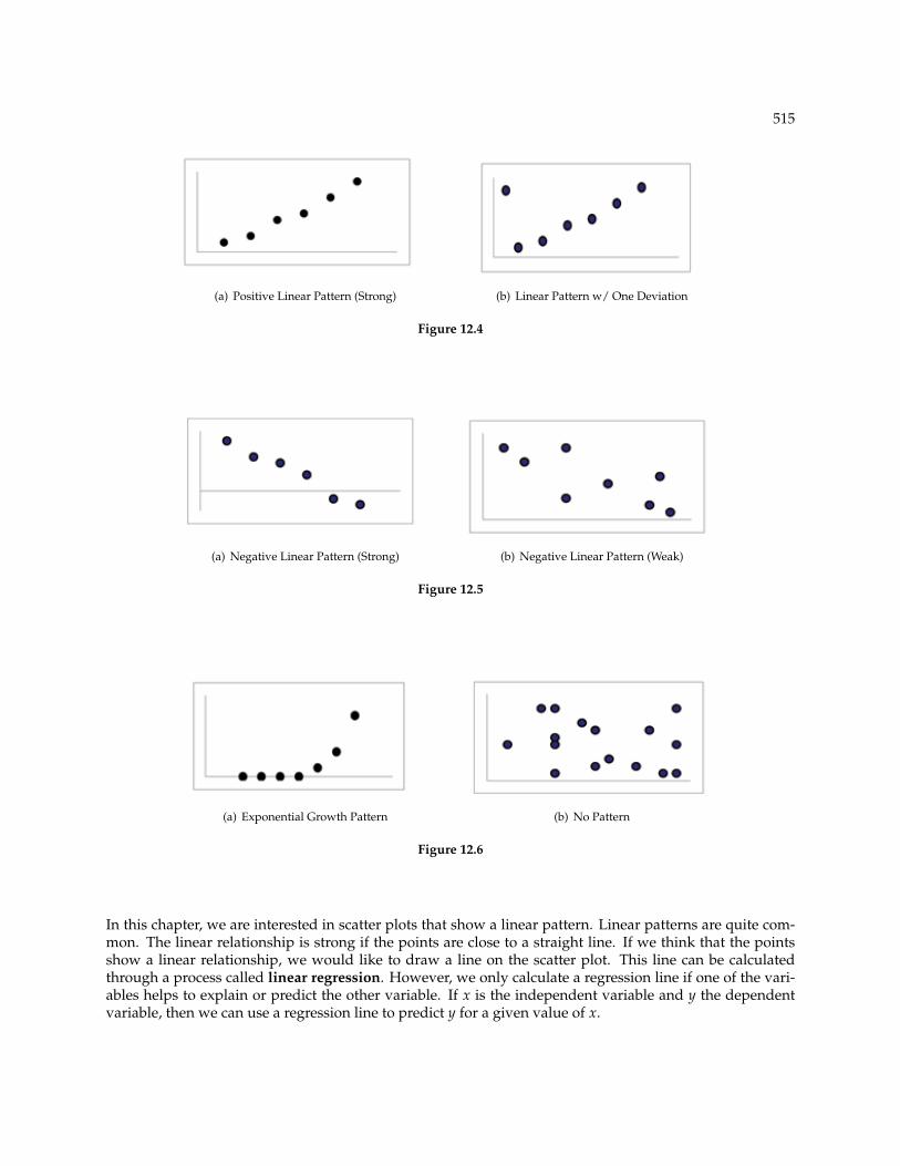
When you look at a scatterplot, you want to notice the overall pattern and any deviations from the pattern.The following scatterplot examples illustrate these concepts.


515

(a) Positive Linear Pattern (Strong) (b) Linear Pattern w/ One Deviation

Figure 12.4

(a) Negative Linear Pattern (Strong) (b) Negative Linear Pattern (Weak)

Figure 12.5

(a) Exponential Growth Pattern (b) No Pattern

Figure 12.6

In this chapter, we are interested in scatter plots that show a linear pattern. Linear patterns are quite com-mon. The linear relationship is strong if the points are close to a straight line. If we think that the pointsshow a linear relationship, we would like to draw a line on the scatter plot. This line can be calculatedthrough a process called linear regression. However, we only calculate a regression line if one of the vari-ables helps to explain or predict the other variable. If x is the independent variable and y the dependentvariable, then we can use a regression line to predict y for a given value of x.


12.5 The Regression Equation5

Data rarely fit a straight line exactly. Usually, you must be satisfied with rough predictions. Typically, youhave a set of data whose scatter plot appears to "fit" a straight line. This is called a Line of Best Fit or LeastSquares Line.

12.5.1 Optional Collaborative Classroom Activity

If you know a person’s pinky (smallest) finger length, do you think you could predict that person’s height?Collect data from your class (pinky finger length, in inches). The independent variable, x, is pinky fingerlength and the dependent variable, y, is height.

For each set of data, plot the points on graph paper. Make your graph big enough and use a ruler. Then"by eye" draw a line that appears to "fit" the data. For your line, pick two convenient points and use themto find the slope of the line. Find the y-intercept of the line by extending your lines so they cross the y-axis.Using the slopes and the y-intercepts, write your equation of "best fit". Do you think everyone will havethe same equation? Why or why not?

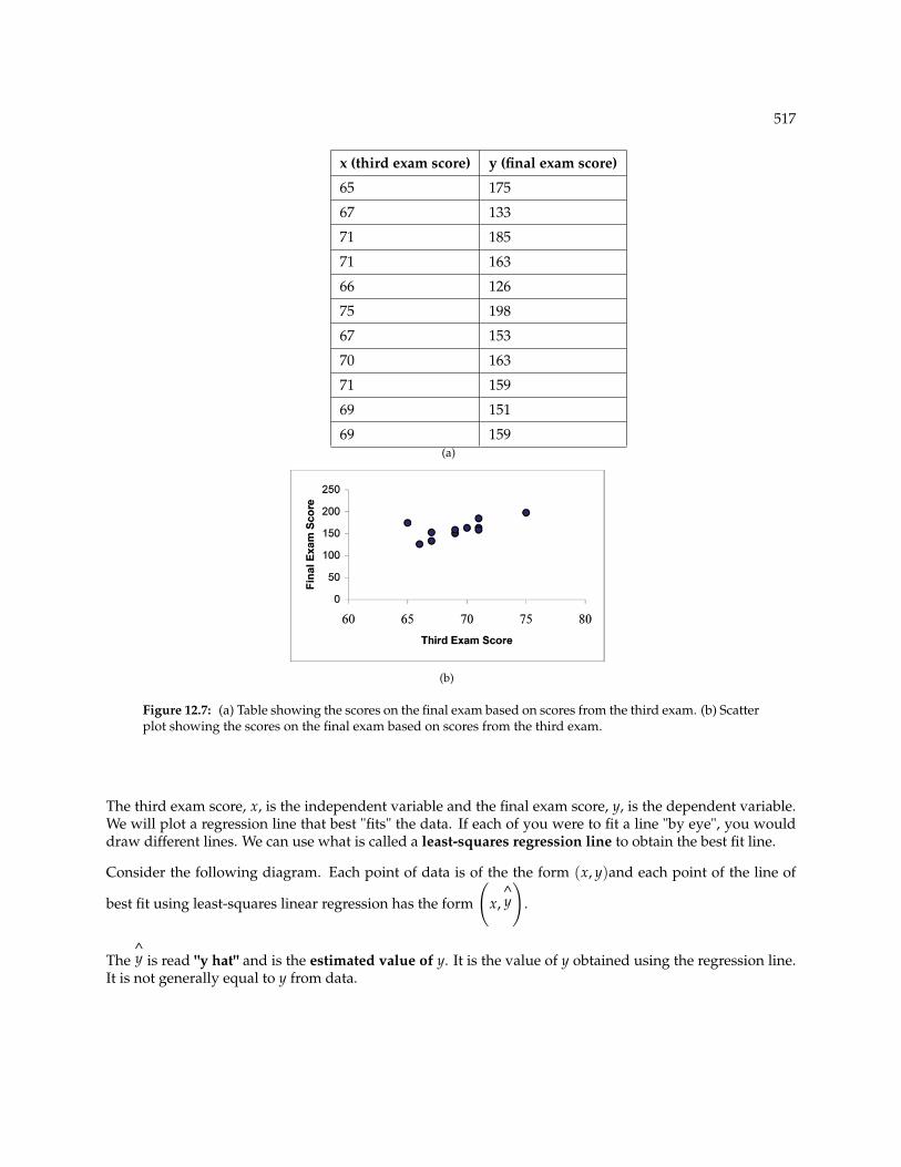
Using your equation, what is the predicted height for a pinky length of 2.5 inches?Example 12.6A random sample of 11 statistics students produced the following data where x is the third examscore, out of 80, and y is the final exam score, out of 200. Can you predict the final exam score of arandom student if you know the third exam score?


517

x (third exam score) y (final exam score)

65 175

67 133

71 185

71 163

66 126

75 198

67 153

70 163

71 159

69 151

69 159(a)

(b)

Figure 12.7: (a) Table showing the scores on the final exam based on scores from the third exam. (b) Scatterplot showing the scores on the final exam based on scores from the third exam.

The third exam score, x, is the independent variable and the final exam score, y, is the dependent variable.We will plot a regression line that best "fits" the data. If each of you were to fit a line "by eye", you woulddraw different lines. We can use what is called a least-squares regression line to obtain the best fit line.

Consider the following diagram. Each point of data is of the the form (x, y)and each point of the line of

best fit using least-squares linear regression has the form

(x,

^y

).

The^y is read "y hat" and is the estimated value of y. It is the value of y obtained using the regression line.

It is not generally equal to y from data.


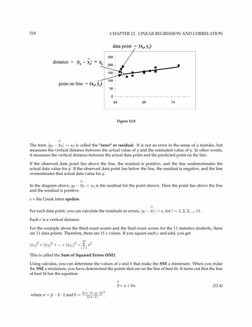
Figure 12.8

The term |y0 −^y0| = ε0 is called the "error" or residual. It is not an error in the sense of a mistake, but

measures the vertical distance between the actual value of y and the estimated value of y. In other words,it measures the vertical distance between the actual data point and the predicted point on the line.

If the observed data point lies above the line, the residual is positive, and the line underestimates theactual data value for y. If the observed data point lies below the line, the residual is negative, and the lineoverestimates that actual data value for y.

In the diagram above, y0 −^y0 = ε0 is the residual for the point shown. Here the point lies above the line

and the residual is positive.

ε = the Greek letter epsilon

For each data point, you can calculate the residuals or errors, |yi −^yi| = εi for i = 1, 2, 3, ..., 11.

Each ε is a vertical distance.

For the example about the third exam scores and the final exam scores for the 11 statistics students, thereare 11 data points. Therefore, there are 11 ε values. If you square each ε and add, you get

(ε1)2 + (ε2)

2 + ... + (ε11)2 =

11Σ

i = 1ε2

This is called the Sum of Squared Errors (SSE).

Using calculus, you can determine the values of a and b that make the SSE a minimum. When you makethe SSE a minimum, you have determined the points that are on the line of best fit. It turns out that the lineof best fit has the equation:

^y= a + bx (12.4)

where a = y− b · x and b = Σ(x−x)·(y−y)Σ(x−x)

2.

519

x and y are the averages of the x values and the y values, respectively. The best fit line always passesthrough the point (x, y).

The slope b can be written as b = r ·(

sysx

)where sy = the standard deviation of the y values and sx = the

standard deviation of the x values. r is the correlation coefficient which is discussed in the next section.

Least Squares Criteria for Best FitThe process of fitting the best fit line is called linear regression. The idea behind finding the best fit line isbased on the assumption that the data are scattered about a straight line. The criteria for the best fit line isthat the sum of the squared errors (SSE) is minimized, that is made as small as possible. Any other line youmight choose would have a higher SSE than the best fit line. This best fit line is called the least squaresregression line .

NOTE: Computer spreadsheets, statistical software, and many calculators can quickly calculate thebest fit line and create the graphs. The calculations tend to be tedious if done by hand. Instructionsto use the TI-83, TI-83+, and TI-84+ calculators to find the best fit line and create a scatterplot areshown at the end of this section.

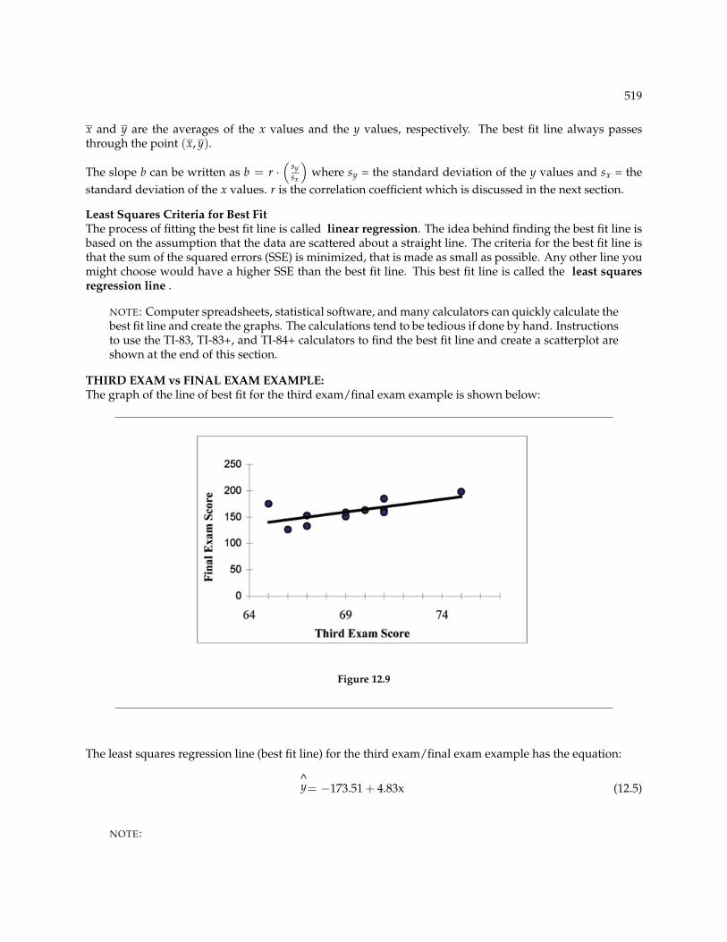
THIRD EXAM vs FINAL EXAM EXAMPLE:The graph of the line of best fit for the third exam/final exam example is shown below:

Figure 12.9

The least squares regression line (best fit line) for the third exam/final exam example has the equation:

^y= −173.51 + 4.83x (12.5)

NOTE:


Remember, it is always important to plot a scatter diagram first. If the scatter plot indicates thatthere is a linear relationship between the variables, then it is reasonable to use a best fit lineto make predictions for y given x within the domain of x-values in the sample data, but notnecessarily for x-values outside that domain.

You could use the line to predict the final exam score for a student who earned a grade of 73 onthe third exam.

You should NOT use the line to predict the final exam score for a student who earned a grade of50 on the third exam, because 50 is not within the domain of the x-values in the sample data,which are between 65 and 75.

UNDERSTANDING SLOPEThe slope of the line, b, describes how changes in the variables are related. It is important to interpretthe slope of the line in the context of the situation represented by the data. You should be able to write asentence interpreting the slope in plain English.

INTERPRETATION OF THE SLOPE: The slope of the best fit line tells us how the dependent variable (y)changes for every one unit increase in the independent (x) variable, on average.THIRD EXAM vs FINAL EXAM EXAMPLE

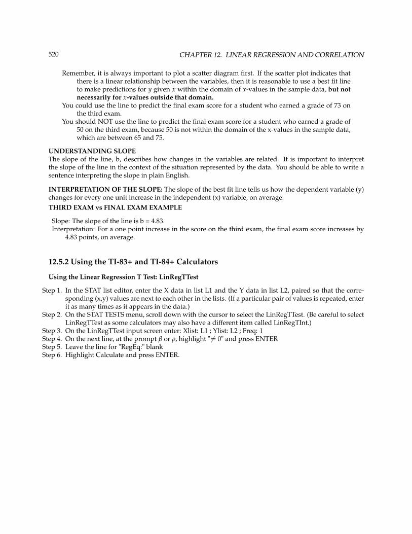
Slope: The slope of the line is b = 4.83.Interpretation: For a one point increase in the score on the third exam, the final exam score increases by

4.83 points, on average.

12.5.2 Using the TI-83+ and TI-84+ Calculators

Using the Linear Regression T Test: LinRegTTest

Step 1. In the STAT list editor, enter the X data in list L1 and the Y data in list L2, paired so that the corre-sponding (x,y) values are next to each other in the lists. (If a particular pair of values is repeated, enterit as many times as it appears in the data.)

Step 2. On the STAT TESTS menu, scroll down with the cursor to select the LinRegTTest. (Be careful to selectLinRegTTest as some calculators may also have a different item called LinRegTInt.)

Step 3. On the LinRegTTest input screen enter: Xlist: L1 ; Ylist: L2 ; Freq: 1Step 4. On the next line, at the prompt β or ρ, highlight " 6= 0" and press ENTERStep 5. Leave the line for "RegEq:" blankStep 6. Highlight Calculate and press ENTER.

521

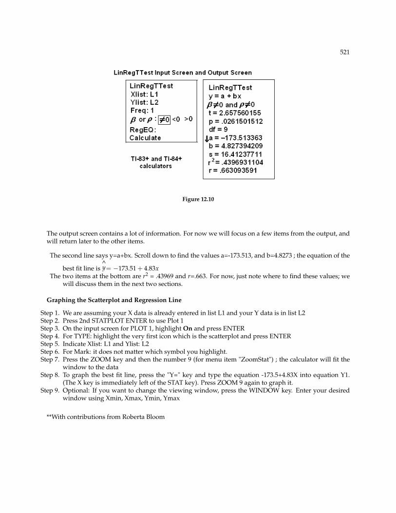
Figure 12.10

The output screen contains a lot of information. For now we will focus on a few items from the output, andwill return later to the other items.

The second line says y=a+bx. Scroll down to find the values a=-173.513, and b=4.8273 ; the equation of the

best fit line is^y= −173.51 + 4.83x

The two items at the bottom are r2 = .43969 and r=.663. For now, just note where to find these values; wewill discuss them in the next two sections.

Graphing the Scatterplot and Regression Line

Step 1. We are assuming your X data is already entered in list L1 and your Y data is in list L2Step 2. Press 2nd STATPLOT ENTER to use Plot 1Step 3. On the input screen for PLOT 1, highlight On and press ENTERStep 4. For TYPE: highlight the very first icon which is the scatterplot and press ENTERStep 5. Indicate Xlist: L1 and Ylist: L2Step 6. For Mark: it does not matter which symbol you highlight.Step 7. Press the ZOOM key and then the number 9 (for menu item "ZoomStat") ; the calculator will fit the

window to the dataStep 8. To graph the best fit line, press the "Y=" key and type the equation -173.5+4.83X into equation Y1.

(The X key is immediately left of the STAT key). Press ZOOM 9 again to graph it.Step 9. Optional: If you want to change the viewing window, press the WINDOW key. Enter your desired

window using Xmin, Xmax, Ymin, Ymax

**With contributions from Roberta Bloom


12.6 Correlation Coefficient and Coefficient of Determination6

12.6.1 The Correlation Coefficient r

Besides looking at the scatter plot and seeing that a line seems reasonable, how can you tell if the line is agood predictor? Use the correlation coefficient as another indicator (besides the scatterplot) of the strengthof the relationship between x and y.

The correlation coefficient, r, developed by Karl Pearson in the early 1900s, is a numerical measure of thestrength of association between the independent variable x and the dependent variable y.

The correlation coefficient is calculated as

r =n · Σx · y− (Σx) · (Σy)√[

n · Σx2 − (Σx)2]·[n · Σy2 − (Σy)2

] (12.6)

where n = the number of data points.

If you suspect a linear relationship between x and y, then r can measure how strong the linear relationshipis.What the VALUE of r tells us:

• The value of r is always between -1 and +1: −1 ≤ r ≤ 1.• The closer the correlation coefficient r is to -1 or 1 (and the further from 0), the stronger the evidence

of a significant linear relationship between x and y; this would indicate that the observed data pointsfit more closely to the best fit line. Values of r further from 0 indicate a stronger linear relationshipbetween x and y. Values of r closer to 0 indicate a weaker linear relationship between x and y.

• If r = 0 there is absolutely no linear relationship between x and y (no linear correlation).• If r = 1, there is perfect positive correlation. If r = −1, there is perfect negative correlation. In both

these cases, all of the original data points lie on a straight line. Of course, in the real world, this willnot generally happen.

What the SIGN of r tells us

• A positive value of r means that when x increases, y increases and when x decreases, y decreases(positive correlation).

• A negative value of r means that when x increases, y decreases and when x decreases, y increases(negative correlation).

• The sign of r is the same as the sign of the slope, b, of the best fit line.

NOTE: Strong correlation does not suggest that x causes y or y causes x. We say "correlation doesnot imply causation." For example, every person who learned math in the 17th century is dead.However, learning math does not necessarily cause death!


523

(a) Positive Correlation (b) Negative Correlation (c) Zero Correlation

Figure 12.11: (a) A scatter plot showing data with a positive correlation. 0 < r < 1 (b) A scatter plotshowing data with a negative correlation. −1 < r < 0 (c) A scatter plot showing data with zero correlation.r=0

The formula for r looks formidable. However, computer spreadsheets, statistical software, and many cal-culators can quickly calculate r. The correlation coefficient r is the bottom item in the output screens for theLinRegTTest on the TI-83, TI-83+, or TI-84+ calculator (see previous section for instructions).

12.6.2 The Coefficient of Determination

r2 is called the coefficient of determination. r2 is the square of the correlation coefficient , but is usuallystated as a percent, rather than in decimal form. r2 has an interpretation in the context of the data

• r2, when expressed as a percent, represents the percent of variation in the dependent variable y thatcan be explained by variation in the independent variable x using the regression (best fit) line.

• 1-r2, when expressed as a percent, represents the percent of variation in y that is NOT explained byvariation in x using the regression line. This can be seen as the scattering of the observed data pointsabout the regression line.

Consider the third exam/final exam example introduced in the previous section

The line of best fit is:^y= −173.51 + 4.83x

The correlation coefficient is r = 0.6631The coefficient of determination is r2 = 0.66312 = 0.4397Interpretation of r2 in the context of this example:

Approximately 44% of the variation in the final exam grades can be explained by the variation in thegrades on the third exam, using the best fit regression line.

Therefore approximately 56% of the variation in the final exam grades can NOT be explained by the vari-ation in the grades on the third exam, using the best fit regression line. (This is seen as the scatteringof the points about the line.)

**With contributions from Roberta Bloom.


12.7 Testing the Significance of the Correlation Coefficient7

12.7.1 Testing the Significance of the Correlation Coefficient

The correlation coefficient, r, tells us about the strength of the linear relationship between x and y. However,the reliability of the linear model also depends on how many observed data points are in the sample. Weneed to look at both the value of the correlation coefficient r and the sample size n, together.

We perform a hypothesis test of the "significance of the correlation coefficient" to decide whether thelinear relationship in the sample data is strong enough and reliable enough to use to model the relationshipin the population.

The sample data is used to compute r, the correlation coefficient for the sample. If we had data for the entirepopulation, we could find the population correlation coefficient. But because we only have sample data, wecan not calculate the population correlation coefficient. The sample correlation coefficient, r, is our estimateof the unknown population correlation coefficient.

The symbol for the population correlation coefficient is ρ, the Greek letter "rho".ρ = population correlation coefficient (unknown)r = sample correlation coefficient (known; calculated from sample data)

The hypothesis test lets us decide whether the value of the population correlation coefficient ρ is "close to0" or "significantly different from 0". We decide this based on the sample correlation coefficient r and thesample size n.If the test concludes that the correlation coefficient is significantly different from 0, we say that thecorrelation coefficient is "significant".

• Conclusion: "The correlation coefficient IS SIGNIFICANT"• What the conclusion means: We believe that there is a significant linear relationship between x and y.

We can use the regression line to model the linear relationship between x and y in the population.

If the test concludes that the correlation coefficient is not significantly different from 0 (it is close to 0),we say that correlation coefficient is "not significant".

• Conclusion: "The correlation coefficient IS NOT SIGNIFICANT."• What the conclusion means: We do NOT believe that there is a significant linear relationship between

x and y. Therefore we can NOT use the regression line to model a linear relationship between x and yin the population.

NOTE:

• If r is significant and the scatter plot shows a reasonable linear trend, the line can be used topredict the value of y for values of x that are within the domain of observed x values.• If r is not significant OR if the scatter plot does not show a reasonable linear trend, the line

should not be used for prediction.• If r is significant and if the scatter plot shows a reasonable linear trend, the line may NOT be

appropriate or reliable for prediction OUTSIDE the domain of observed x values in the data.

PERFORMING THE HYPOTHESIS TESTSETTING UP THE HYPOTHESES:

• Null Hypothesis: Ho: ρ=0


525

• Alternate Hypothesis: Ha: ρ 6=0

What the hypotheses mean in words:

• Null Hypothesis Ho: The population correlation coefficient IS NOT significantly different from 0.There IS NOT a significant linear relationship(correlation) between x and y in the population.

• Alternate Hypothesis Ha: The population correlation coefficient IS significantly DIFFERENT FROM0. There IS A SIGNIFICANT LINEAR RELATIONSHIP (correlation) between x and y in the popula-tion.

DRAWING A CONCLUSION:

There are two methods to make the decision. Both methods are equivalent and give the same result.Method 1: Using the p-valueMethod 2: Using a table of critical valuesIn this chapter of this textbook, we will always use a significance level of 5%, α = 0.05Note: Using the p-value method, you could choose any appropriate significance level you want; you are

not limited to using α = 0.05. But the table of critical values provided in this textbook assumes thatwe are using a significance level of 5%, α = 0.05. (If we wanted to use a different significance levelthan 5% with the critical value method, we would need different tables of critical values that are notprovided in this textbook.)

METHOD 1: Using a p-value to make a decision

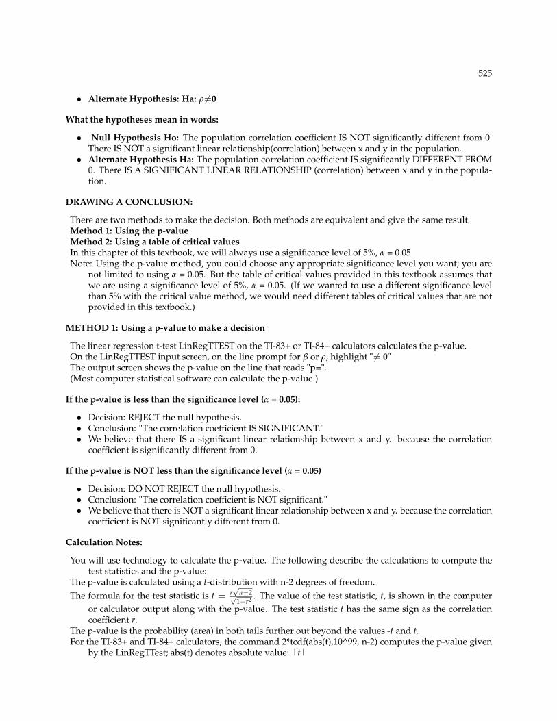
The linear regression t-test LinRegTTEST on the TI-83+ or TI-84+ calculators calculates the p-value.On the LinRegTTEST input screen, on the line prompt for β or ρ, highlight " 6= 0"The output screen shows the p-value on the line that reads "p=".(Most computer statistical software can calculate the p-value.)

If the p-value is less than the significance level (α = 0.05):

• Decision: REJECT the null hypothesis.• Conclusion: "The correlation coefficient IS SIGNIFICANT."• We believe that there IS a significant linear relationship between x and y. because the correlation

coefficient is significantly different from 0.

If the p-value is NOT less than the significance level (α = 0.05)

• Decision: DO NOT REJECT the null hypothesis.• Conclusion: "The correlation coefficient is NOT significant."• We believe that there is NOT a significant linear relationship between x and y. because the correlation

coefficient is NOT significantly different from 0.

Calculation Notes:

You will use technology to calculate the p-value. The following describe the calculations to compute thetest statistics and the p-value:

The p-value is calculated using a t-distribution with n-2 degrees of freedom.The formula for the test statistic is t = r

√n−2√

1−r2 . The value of the test statistic, t, is shown in the computeror calculator output along with the p-value. The test statistic t has the same sign as the correlationcoefficient r.

The p-value is the probability (area) in both tails further out beyond the values -t and t.For the TI-83+ and TI-84+ calculators, the command 2*tcdf(abs(t),10^99, n-2) computes the p-value given

by the LinRegTTest; abs(t) denotes absolute value: |t|


THIRD EXAM vs FINAL EXAM EXAMPLE: p value method

• Consider the third exam/final exam example.

• The line of best fit is:^y= −173.51 + 4.83x with r = 0.6631 and there are n = 11 data points.

• Can the regression line be used for prediction? Given a third exam score (x value), can we use theline to predict the final exam score (predicted y value)?

Ho: ρ = 0Ha: ρ 6= 0α = 0.05The p-value is 0.026 (from LinRegTTest on your calculator or from computer software)The p-value, 0.026, is less than the significance level of α = 0.05Decision: Reject the Null Hypothesis HoConclusion: The correlation coefficient IS SIGNIFICANT.Because r is significant and the scatter plot shows a reasonable linear trend, the regression line can be

used to predict final exam scores.

METHOD 2: Using a table of Critical Values to make a decisionThe 95% Critical Values of the Sample Correlation Coefficient Table (Section 12.10) at the end of thischapter (before the Summary (Section 12.11)) may be used to give you a good idea of whether the com-puted value of r is significant or not. Compare r to the appropriate critical value in the table. If r is notbetween the positive and negative critical values, then the correlation coefficient is significant. If r is signif-icant, then you may want to use the line for prediction.

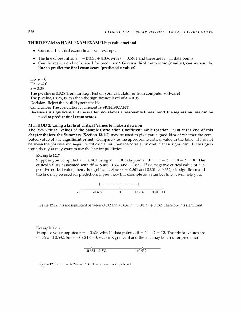
Example 12.7Suppose you computed r = 0.801 using n = 10 data points. df = n − 2 = 10 − 2 = 8. Thecritical values associated with df = 8 are -0.632 and + 0.632. If r< negative critical value or r >positive critical value, then r is significant. Since r = 0.801 and 0.801 > 0.632, r is significant andthe line may be used for prediction. If you view this example on a number line, it will help you.

Figure 12.12: r is not significant between -0.632 and +0.632. r = 0.801 > + 0.632. Therefore, r is significant.

Example 12.8Suppose you computed r = −0.624 with 14 data points. df = 14− 2 = 12. The critical values are

-0.532 and 0.532. Since −0.624<−0.532, r is significant and the line may be used for prediction

Figure 12.13: r = −0.624<−0.532. Therefore, r is significant.

527

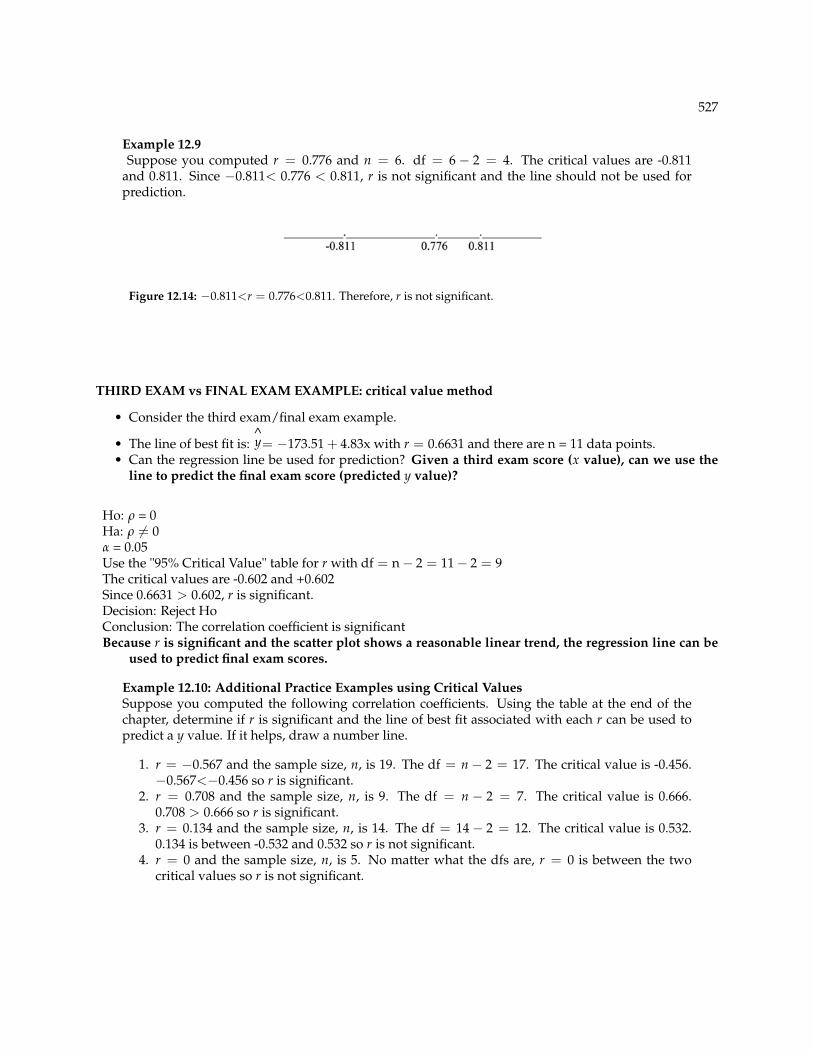
Example 12.9Suppose you computed r = 0.776 and n = 6. df = 6 − 2 = 4. The critical values are -0.811

and 0.811. Since −0.811< 0.776 < 0.811, r is not significant and the line should not be used forprediction.

Figure 12.14: −0.811<r = 0.776<0.811. Therefore, r is not significant.

THIRD EXAM vs FINAL EXAM EXAMPLE: critical value method

• Consider the third exam/final exam example.

• The line of best fit is:^y= −173.51 + 4.83x with r = 0.6631 and there are n = 11 data points.

• Can the regression line be used for prediction? Given a third exam score (x value), can we use theline to predict the final exam score (predicted y value)?

Ho: ρ = 0Ha: ρ 6= 0α = 0.05Use the "95% Critical Value" table for r with df = n− 2 = 11− 2 = 9The critical values are -0.602 and +0.602Since 0.6631 > 0.602, r is significant.Decision: Reject HoConclusion: The correlation coefficient is significantBecause r is significant and the scatter plot shows a reasonable linear trend, the regression line can be

used to predict final exam scores.

Example 12.10: Additional Practice Examples using Critical ValuesSuppose you computed the following correlation coefficients. Using the table at the end of thechapter, determine if r is significant and the line of best fit associated with each r can be used topredict a y value. If it helps, draw a number line.

1. r = −0.567 and the sample size, n, is 19. The df = n− 2 = 17. The critical value is -0.456.−0.567<−0.456 so r is significant.

2. r = 0.708 and the sample size, n, is 9. The df = n − 2 = 7. The critical value is 0.666.0.708 > 0.666 so r is significant.

3. r = 0.134 and the sample size, n, is 14. The df = 14− 2 = 12. The critical value is 0.532.0.134 is between -0.532 and 0.532 so r is not significant.

4. r = 0 and the sample size, n, is 5. No matter what the dfs are, r = 0 is between the twocritical values so r is not significant.


12.7.2 Assumptions in Testing the Significance of the Correlation Coefficient

Testing the significance of the correlation coefficient requires that certain assumptions about the data aresatisfied. The premise of this test is that the data are a sample of observed points taken from a largerpopulation. We have not examined the entire population because it is not possible or feasible to do so. Weare examining the sample to draw a conclusion about whether the linear relationship that we see betweenx and y in the sample data provides strong enough evidence so that we can conclude that there is a linearrelationship between x and y in the population.

The regression line equation that we calculate from the sample data gives the best fit line for our particularsample. We want to use this best fit line for the sample as an estimate of the best fit line for the population.Examining the scatterplot and testing the significance of the correlation coefficient helps us determine if itis appropriate to do this.The assumptions underlying the test of significance are:

• There is a linear relationship in the population that models the average value of y for varying valuesof x. In other words, the average of the y values for each particular x value lie on a straight linein the population. (We do not know the equation for the line for the population. Our regression linefrom the sample is our best estimate of this line in the population.)

• The y values for any particular x value are normally distributed about the line. This implies thatthere are more y values scattered closer to the line than are scattered farther away. Assumption (1)above implies that these normal distributions are centered on the line: the means of these normaldistributions of y values lie on the line.

• The standard deviations of the population y values about the line the equal for each value of x. Inother words, each of these normal distributions of y values has the same shape and spread about theline.

Figure 12.15: The y values for each x value are normally distributed about the line with the same standarddeviation. For each x value, the mean of the y values lies on the regression line. More y values lie near theline than are scattered further away from the line.


529

12.8 Prediction8

Recall the third exam/final exam example.

We examined the scatterplot and showed that the correlation coefficient is significant. We found the equa-tion of the best fit line for the final exam grade as a function of the grade on the third exam. We can nowuse the least squares regression line for prediction.

Suppose you want to estimate, or predict, the final exam score of statistics students who received 73 on thethird exam. The exam scores (x-values) range from 65 to 75. Since 73 is between the x-values 65 and 75,substitute x = 73 into the equation. Then:

^y= −173.51 + 4.83 (73) = 179.08 (12.8)

We predict that statistic students who earn a grade of 73 on the third exam will earn a grade of 179.08 onthe final exam, on average.

Example 12.11Recall the third exam/final exam example.Problem 1What would you predict the final exam score to be for a student who scored a 66 on the third

exam?

Solution145.27

Problem 2 (Solution on p. 566.)What would you predict the final exam score to be for a student who scored a 78 on the third

exam?


12.9 Outliers9

In some data sets, there are values (observed data points) called outliers. Outliers are observed datapoints that are far from the least squares line. They have large "errors", where the "error" or residual is thevertical distance from the line to the point.

Outliers need to be examined closely. Sometimes, for some reason or another, they should not be includedin the analysis of the data. It is possible that an outlier is a result of erroneous data. Other times, an outliermay hold valuable information about the population under study and should remain included in the data.The key is to carefully examine what causes a data point to be an outlier.

Besides outliers, a sample may contain one or a few points that are called influential points. Influentialpoints are observed data points that are far from the other observed data points but that greatly influencethe line. As a result an influential point may be close to the line, even though it is far from the rest of thedata. Because an influential point so strongly influences the best fit line, it generally will not have a large"error" or residual.

8This content is available online at <http://http://cnx.org/content/m17095/1.7/>.9This content is available online at <http://http://cnx.org/content/m17094/1.13/>.


Computers and many calculators can be used to identify outliers from the data. Computer output forregression analysis will often identify both outliers and influential points so that you can examine them.

Identifying OutliersWe could guess at outliers by looking at a graph of the scatterplot and best fit line. However we would likesome guideline as to how far away a point needs to be in order to be considered an outlier. As a rough ruleof thumb, we can flag any point that is located further than two standard deviations above or below thebest fit line as an outlier. The standard deviation used is the standard deviation of the residuals or errors.

We can do this visually in the scatterplot by drawing an extra pair of lines that are two standard deviationsabove and below the best fit line. Any data points that are outside this extra pair of lines are flagged aspotential outliers. Or we can do this numerically by calculating each residual and comparing it to twice thestandard deviation. On the TI-83, 83+, or 84+, the graphical approach is easier. The graphical procedureis shown first, followed by the numerical calculations. You would generally only need to use one of thesemethods.

Example 12.12In the third exam/final exam example, you can determine if there is an outlier or not. If there is

an outlier, as an exercise, delete it and fit the remaining data to a new line. For this example, thenew line ought to fit the remaining data better. This means the SSE should be smaller and thecorrelation coefficient ought to be closer to 1 or -1.

SolutionGraphical Identification of Outliers

With the TI-83,83+,84+ graphing calculators, it is easy to identify the outlier graphically and visu-ally. If we were to measure the vertical distance from any data point to the corresponding pointon the line of best fit and that distance was equal to 2s or farther, then we would consider the datapoint to be "too far" from the line of best fit. We need to find and graph the lines that are twostandard deviations below and above the regression line. Any points that are outside these twolines are outliers. We will call these lines Y2 and Y3:

As we did with the equation of the regression line and the correlation coefficient, we will usetechnology to calculate this standard deviation for us. Using the LinRegTTest with this data,scroll down through the output screens to find s=16.412

Line Y2=-173.5+4.83x-2(16.4) and line Y3=-173.5+4.83X+2(16.4)

where^y=-173.5+4.83x is the line of best fit. Y2 and Y3 have the same slope as the line of

best fit.

Graph the scatterplot with the best fit line in equation Y1, then enter the two extra lines as Y2 andY3 in the "Y="equation editor and press ZOOM 9. You will find that the only data point that is notbetween lines Y2 and Y3 is the point x=65, y=175. On the calculator screen it is just barely outsidethese lines. The outlier is the student who had a grade of 65 on the third exam and 175 on the finalexam; this point is further than 2 standard deviations away from the best fit line.

Sometimes a point is so close to the lines used to flag outliers on the graph that it is difficult totell if the point is between or outside the lines. On a computer, enlarging the graph may help; ona small calculator screen, zooming in may make the graph more clear. Note that when the graphdoes not give a clear enough picture, you can use the numerical comparisons to identify outliers.

531

Figure 12.16

Numerical Identification of OutliersIn the table below, the first two columns are the third exam and final exam data. The third

column shows the predicted^y values calculated from the line of best fit:

^y=-173.5+4.83x. The

residuals, or errors, have been calculated in the fourth column of the table: observed y value−

predicted y value = y−^y.

s is the standard deviation of all the y−^y= ε values where n = the total number of data points. If

each residual is calculated and squared, and the results are added up, we get the SSE. The standarddeviation of the residuals is calculated from the SSE as:

s =√

SSEn−2

Rather than calculate the value of s ourselves, we can find s using the computer or calculator. Forthis example, our calculator LinRegTTest found s=16.4 as the standard deviation of the residuals:35; -17; 16; -6; -19; 9; 3; -1; -10; -9; -1.


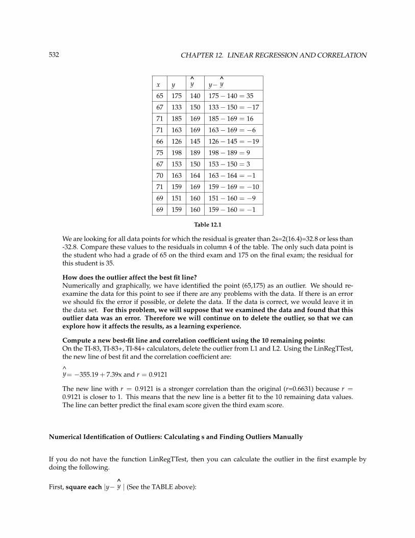
x y^y y−

^y

65 175 140 175− 140 = 35

67 133 150 133− 150 = −17

71 185 169 185− 169 = 16

71 163 169 163− 169 = −6

66 126 145 126− 145 = −19

75 198 189 198− 189 = 9

67 153 150 153− 150 = 3

70 163 164 163− 164 = −1

71 159 169 159− 169 = −10

69 151 160 151− 160 = −9

69 159 160 159− 160 = −1

Table 12.1

We are looking for all data points for which the residual is greater than 2s=2(16.4)=32.8 or less than-32.8. Compare these values to the residuals in column 4 of the table. The only such data point isthe student who had a grade of 65 on the third exam and 175 on the final exam; the residual forthis student is 35.

How does the outlier affect the best fit line?Numerically and graphically, we have identified the point (65,175) as an outlier. We should re-examine the data for this point to see if there are any problems with the data. If there is an errorwe should fix the error if possible, or delete the data. If the data is correct, we would leave it inthe data set. For this problem, we will suppose that we examined the data and found that thisoutlier data was an error. Therefore we will continue on to delete the outlier, so that we canexplore how it affects the results, as a learning experience.

Compute a new best-fit line and correlation coefficient using the 10 remaining points:On the TI-83, TI-83+, TI-84+ calculators, delete the outlier from L1 and L2. Using the LinRegTTest,the new line of best fit and the correlation coefficient are:

^y= −355.19 + 7.39x and r = 0.9121

The new line with r = 0.9121 is a stronger correlation than the original (r=0.6631) because r =0.9121 is closer to 1. This means that the new line is a better fit to the 10 remaining data values.The line can better predict the final exam score given the third exam score.

Numerical Identification of Outliers: Calculating s and Finding Outliers Manually

If you do not have the function LinRegTTest, then you can calculate the outlier in the first example bydoing the following.

First, square each |y−^y | (See the TABLE above):

533

The squares are 352; 172; 162; 62; 192; 92; 32; 12; 102; 92; 12

Then, add (sum) all the |y−^y | squared terms using the formula

11Σ

i = 1

(|yi −

^yi|)2

=11Σ

i = 1εi

2 (Recall that |yi −^yi| = εi.)

= 352 + 172 + 162 + 62 + 192 + 92 + 32 + 12 + 102 + 92 + 12

= 2440 = SSE. The result, SSE is the Sum of Squared Errors.

Next, calculate s, the standard deviation of all the |y−^y | = ε values where n = the total number of data

points. (Calculate the standard deviation of 35; 17; 16; 6; 19; 9; 3; 1; 10; 9; 1.)

The calculation is s =√

SSEn−2

For the third exam/final exam problem, s =√

244011−2 = 16.47

Next, multiply s by 1.9:(1.9) · (16.47) = 31.29

31.29 is almost 2 standard deviations away from the mean of the |y−^y | values.

If we were to measure the vertical distance from any data point to the corresponding point on the line ofbest fit and that distance is at least 1.9s, then we would consider the data point to be "too far" from the lineof best fit. We call that point a potential outlier.

For the example, if any of the |y−^y | values are at least 31.29, the corresponding (x, y) data point is a

potential outlier.

For the third exam/final exam problem, all the |y−^y |’s are less than 31.29 except for the first one which is

35.

35 > 31.29 That is, |y−^y | ≥ (1.9) · (s)

The point which corresponds to |y−^y | = 35 is (65, 175). Therefore, the data point (65, 175) is a potential

outlier. For this example, we will delete it. (Remember, we do not always delete an outlier.)

The next step is to compute a new best-fit line using the 10 remaining points. The new line of bestfit and the correlation coefficient are:

^y= −355.19 + 7.39x and r = 0.9121

Example 12.13Using this new line of best fit (based on the remaining 10 data points), what would a student

who receives a 73 on the third exam expect to receive on the final exam? Is this the same as theprediction made using the original line?


Solution

Using the new line of best fit,^y= −355.19 + 7.39(73) = 184.28. A student who scored 73 points on

the third exam would expect to earn 184 points on the final exam.

The original line predicted^y= −173.51 + 4.83(73) = 179.08 so the prediction using the new

line with the outlier eliminated differs from the original prediction.

Example 12.14(From The Consumer Price Indexes Web site) The Consumer Price Index (CPI) measures the aver-age change over time in the prices paid by urban consumers for consumer goods and services. TheCPI affects nearly all Americans because of the many ways it is used. One of its biggest uses is asa measure of inflation. By providing information about price changes in the Nation’s economy togovernment, business, and labor, the CPI helps them to make economic decisions. The President,Congress, and the Federal Reserve Board use the CPI’s trends to formulate monetary and fiscalpolicies. In the following table, x is the year and y is the CPI.

Data:

x y

1915 10.1

1926 17.7

1935 13.7

1940 14.7

1947 24.1

1952 26.5

1964 31.0

1969 36.7

1975 49.3

1979 72.6

1980 82.4

1986 109.6

1991 130.7

1999 166.6

Table 12.2

Problem

• Make a scatterplot of the data.

• Calculate the least squares line. Write the equation in the form^y= a + bx.

• Draw the line on the scatterplot.• Find the correlation coefficient. Is it significant?• What is the average CPI for the year 1990?

535

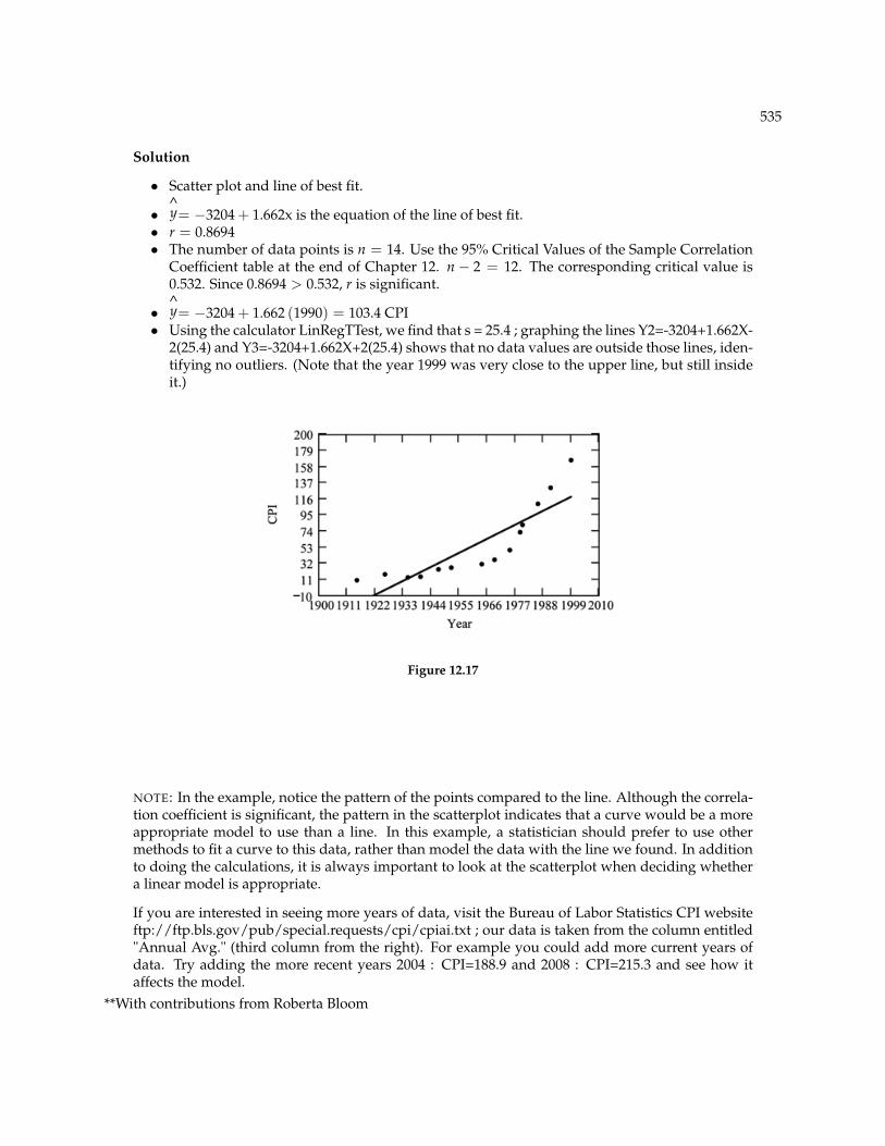
Solution

• Scatter plot and line of best fit.

•^y= −3204 + 1.662x is the equation of the line of best fit.

• r = 0.8694• The number of data points is n = 14. Use the 95% Critical Values of the Sample Correlation

Coefficient table at the end of Chapter 12. n − 2 = 12. The corresponding critical value is0.532. Since 0.8694 > 0.532, r is significant.

•^y= −3204 + 1.662 (1990) = 103.4 CPI

• Using the calculator LinRegTTest, we find that s = 25.4 ; graphing the lines Y2=-3204+1.662X-2(25.4) and Y3=-3204+1.662X+2(25.4) shows that no data values are outside those lines, iden-tifying no outliers. (Note that the year 1999 was very close to the upper line, but still insideit.)

Figure 12.17

NOTE: In the example, notice the pattern of the points compared to the line. Although the correla-tion coefficient is significant, the pattern in the scatterplot indicates that a curve would be a moreappropriate model to use than a line. In this example, a statistician should prefer to use othermethods to fit a curve to this data, rather than model the data with the line we found. In additionto doing the calculations, it is always important to look at the scatterplot when deciding whethera linear model is appropriate.

If you are interested in seeing more years of data, visit the Bureau of Labor Statistics CPI websiteftp://ftp.bls.gov/pub/special.requests/cpi/cpiai.txt ; our data is taken from the column entitled"Annual Avg." (third column from the right). For example you could add more current years ofdata. Try adding the more recent years 2004 : CPI=188.9 and 2008 : CPI=215.3 and see how itaffects the model.



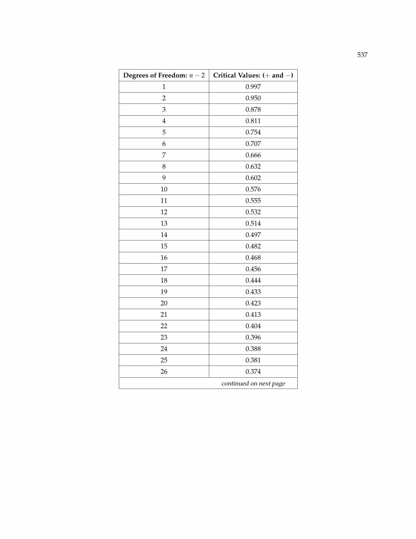
12.10 95% Critical Values of the Sample Correlation Coefficient Table10


537

Degrees of Freedom: n− 2 Critical Values: (+ and −)

1 0.997

2 0.950

3 0.878

4 0.811

5 0.754

6 0.707

7 0.666

8 0.632

9 0.602

10 0.576

11 0.555

12 0.532

13 0.514

14 0.497

15 0.482

16 0.468

17 0.456

18 0.444

19 0.433

20 0.423

21 0.413

22 0.404

23 0.396

24 0.388

25 0.381

26 0.374

continued on next page


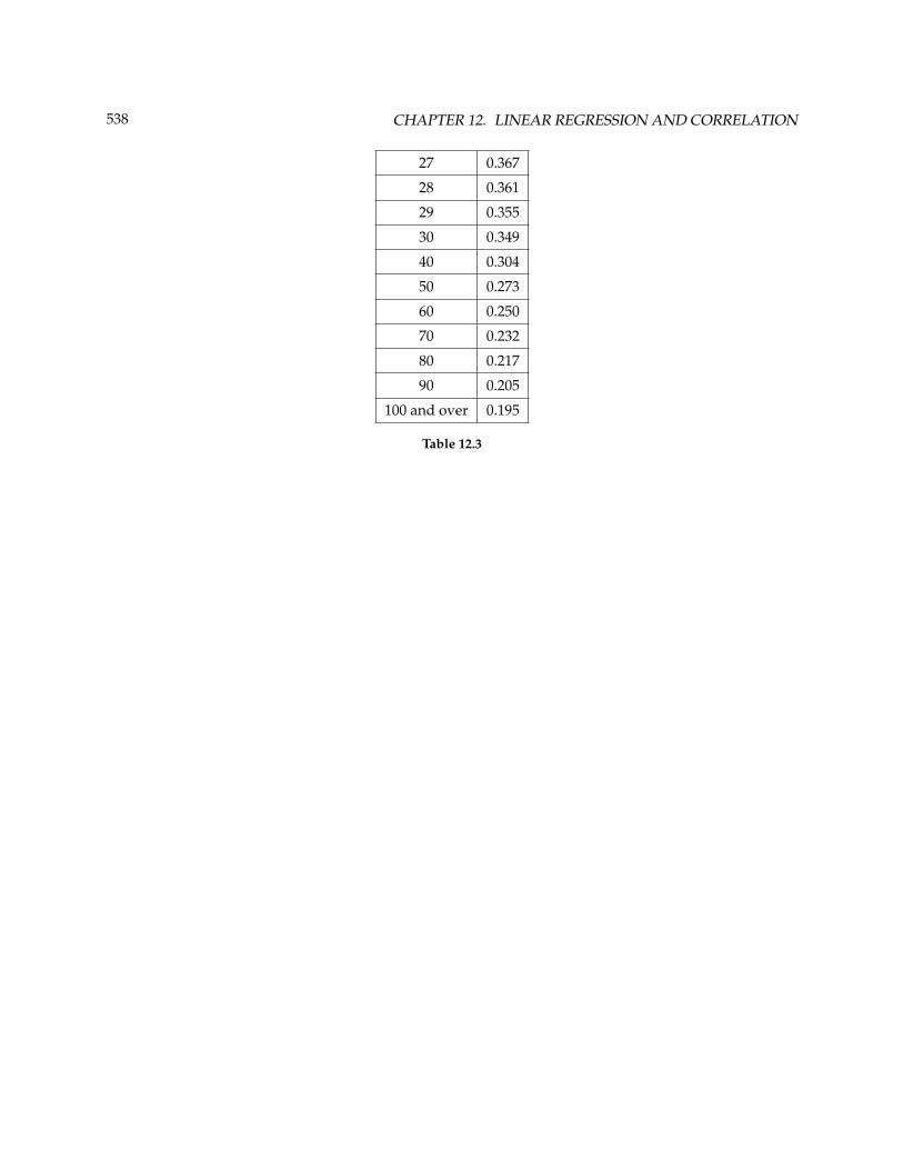
27 0.367

28 0.361

29 0.355

30 0.349

40 0.304

50 0.273

60 0.250

70 0.232

80 0.217

90 0.205

100 and over 0.195

Table 12.3

539

12.11 Summary11

Bivariate Data: Each data point has two values. The form is (x, y).

Line of Best Fit or Least Squares Line (LSL):^y= a + bx

x = independent variable; y = dependent variable

Residual: Actual y value− predicted y value = y−^y

Correlation Coefficient r:

1. Used to determine whether a line of best fit is good for prediction.2. Between -1 and 1 inclusive. The closer r is to 1 or -1, the closer the original points are to a straight line.3. If r is negative, the slope is negative. If r is positive, the slope is positive.4. If r = 0, then the line is horizontal.

Sum of Squared Errors (SSE): The smaller the SSE, the better the original set of points fits the line of bestfit.

Outlier: A point that does not seem to fit the rest of the data.


Linear Regression and Correlation - · PDF fileLinear Regression and Correlation ... is there...

Documents

Transcript of Linear Regression and Correlation - · PDF fileLinear Regression and Correlation ... is there...