Linear Quadratic Optimal Control of an Inverted Pendulum...
16
Çukurova Üniversitesi Mühendislik Mimarlık Fakültesi Dergisi, 32(2), ss. 109-123, Haziran 2017 Çukurova University Journal of the Faculty of Engineering and Architecture, 32(2), pp. 109-123, June 2017 Ç.Ü. Müh. Mim. Fak. Dergisi, 32(2), Haziran 2017 109 Linear Quadratic Optimal Control of an Inverted Pendulum on a Cart using Artificial Bee Colony Algorithm: An Experimental Study Barış ATA 1 , Ramazan ÇOBAN *1 1 Çukurova Üniversitesi, Mühendislik Mimarlık Fakültesi, Bilgisayar Mühendisliği Bölümü, Adana Geliş tarihi: 07.02.2017 Kabul tarihi: 31.05.2017 Abstract This study presents a Linear Quadratic Optimal (LQR) controller design for an inverted pendulum on a cart using the Artificial Bee Colony (ABC) algorithm. Main design parameters of the linear quadratic regulator are the weighting matrices. Generally, selecting weighting matrices is managed by trial and error since there exists no apparent connection between these weights and time domain requirements such as settling time, steady state error, and overshoot percentage. In this study after deriving the mathematical models of the inverted pendulum on a cart and the DC motor, an LQR controller is designed using the ABC algorithm to determine weighting matrices to overcome LQR design difficulties. The comparison and experimental results justify that the ABC algorithm is a very efficient way to determine LQR weighting matrices in comparison with a method in literature. Keywords: Artificial bee colony algorithm, Linear quadratic regulator, Inverted pendulum Yapay Arı Kolonisi Algoritması ile Bir Arabalı Ters Sarkacın Lineer Kuadratik Kontrolü: Deneysel Bir Çalışma Öz Bu çalışmada, Lineer Kuadratik Regülatör (LQR) ile bir ters sarkacın kontrolü için, Yapay Arı Kolonisi (ABC) optimizasyon algoritmasına dayalı bir metot önerilmiştir. LQR’ın temel tasarım parametreleri ağırlık matrisleridir. Ağırlık matrislerinin değerleri ile yüzde aşımı, yerleşme zamanı ve kararlı hal hatası gibi zaman uzayı performans kriterleri arasında doğrudan bir ilişki olmadığı için bu matrislerin seçimi genellikle deneme yanılma yöntemiyle gerçekleştirilmektedir. Bu çalışmada arabalı ters sarkaç ve bu mekanizmayı hareket ettiren DC motorun matematiksel modellerinin elde edilmesinin ardından sürü zekası temelli bir optimizasyon algoritması olan ABC algoritması kullanılarak bir LQR kontrolör tasarlanmıştır. Karşılaştırma ve deney sonuçları, ABC algoritmasının literatürde önerilen bir yöntem ile karşılaştırıldığında ağırlık matrislerinin belirlenmesinde daha etkin bir yol olduğunu göstermiştir. Anahtar Kelimeler: Yapay arı kolonisi algoritması, Lineer kuadratik regülatör, Ters sarkaç * Sorumlu yazar (Corresponding author): Ramazan Çoban, [email protected]
Transcript of Linear Quadratic Optimal Control of an Inverted Pendulum...

Çukurova Üniversitesi Mühendislik Mimarlık Fakültesi Dergisi, 32(2), ss. 109-123, Haziran 2017 Çukurova University Journal of the Faculty of Engineering and Architecture, 32(2), pp. 109-123, June 2017
Ç.Ü. Müh. Mim. Fak. Dergisi, 32(2), Haziran 2017 109
Linear Quadratic Optimal Control of an Inverted Pendulum on a Cart
using Artificial Bee Colony Algorithm: An Experimental Study
Barış ATA1, Ramazan ÇOBAN
*1
1Çukurova Üniversitesi, Mühendislik Mimarlık Fakültesi, Bilgisayar Mühendisliği Bölümü,
Adana
Geliş tarihi: 07.02.2017 Kabul tarihi: 31.05.2017
Abstract
This study presents a Linear Quadratic Optimal (LQR) controller design for an inverted pendulum on a
cart using the Artificial Bee Colony (ABC) algorithm. Main design parameters of the linear quadratic
regulator are the weighting matrices. Generally, selecting weighting matrices is managed by trial and
error since there exists no apparent connection between these weights and time domain requirements such
as settling time, steady state error, and overshoot percentage. In this study after deriving the mathematical
models of the inverted pendulum on a cart and the DC motor, an LQR controller is designed using the
ABC algorithm to determine weighting matrices to overcome LQR design difficulties. The comparison
and experimental results justify that the ABC algorithm is a very efficient way to determine LQR
weighting matrices in comparison with a method in literature.
Keywords: Artificial bee colony algorithm, Linear quadratic regulator, Inverted pendulum
Yapay Arı Kolonisi Algoritması ile Bir Arabalı Ters Sarkacın Lineer Kuadratik
Kontrolü: Deneysel Bir Çalışma
Öz
Bu çalışmada, Lineer Kuadratik Regülatör (LQR) ile bir ters sarkacın kontrolü için, Yapay Arı Kolonisi
(ABC) optimizasyon algoritmasına dayalı bir metot önerilmiştir. LQR’ın temel tasarım parametreleri
ağırlık matrisleridir. Ağırlık matrislerinin değerleri ile yüzde aşımı, yerleşme zamanı ve kararlı hal hatası
gibi zaman uzayı performans kriterleri arasında doğrudan bir ilişki olmadığı için bu matrislerin seçimi
genellikle deneme yanılma yöntemiyle gerçekleştirilmektedir. Bu çalışmada arabalı ters sarkaç ve bu
mekanizmayı hareket ettiren DC motorun matematiksel modellerinin elde edilmesinin ardından sürü
zekası temelli bir optimizasyon algoritması olan ABC algoritması kullanılarak bir LQR kontrolör
tasarlanmıştır. Karşılaştırma ve deney sonuçları, ABC algoritmasının literatürde önerilen bir yöntem ile
karşılaştırıldığında ağırlık matrislerinin belirlenmesinde daha etkin bir yol olduğunu göstermiştir.
Anahtar Kelimeler: Yapay arı kolonisi algoritması, Lineer kuadratik regülatör, Ters sarkaç
*Sorumlu yazar (Corresponding author): Ramazan Çoban, [email protected]
Linear Quadratic Optimal Control of an Inverted Pendulum on a Cart Using Artificial Bee Colony Algorithm: An
Experimental Study
110 Ç.Ü. Müh. Mim. Fak. Dergisi, 32(2), Haziran 2017
1. INTRODUCTION
Controlling an inverted pendulum on a cart is a
challenging problem due to the various characters
of the system: including highly unstable,
nonlinear, non-minimum phase, underactuated,
and single input-two output mechanical system.
Several substantial control systems can be
modelled with the help of inverted pendulum [1].
Inverted pendulum reveals many interesting
system - theoretic properties and its dynamics are
fundamental for balancing problems [2,3].
The inverted pendulum system set up consists of a
cart, a pendulum, a DC motor, and a driving
mechanism. There are two equilibrium points
being stable (downwards position) and unstable
(upwards position) for this system. Hence, there
are two control objectives for the inverted
pendulum system. First one is to swing the
pendulum up to unstable equilibrium from stable
equilibrium and the second one is to maintain the
unstable equilibrium position. This study will
focus on the design of an optimal controller for the
second control objective for the inverted pendulum
system. During this study Feedback Instruments’
digital pendulum system [4] is used to create a
more realistic control system.
One of the widely used optimal control techniques
is the Linear Quadratic Regulator (LQR) [5, 6].
The challenging part of the LQR controller design
is to choose its weights for states and control
signal [7]. Generally selecting these matrices is
based on the knowledge of control engineers or
designers and this process takes a long time since
it is carried out by trial and error. Various methods
to determine suitable weighting matrices have been
proposed [5, 8]. One of the methods for choosing
weighting matrices for LQR is Bryson’s rules [9].
According to this method 𝑄 can be taken as
Q=CTQC. Since matrix 𝐶 includes important
outputs, these states are included within the cost.
Also another method for choosing weighting
matrices for linear quadratic control of an inverted
pendulum is proposed by Ghosh et al. [10].
According to this method, the 𝑄 matrix can be
chosen as 𝑄 = 𝑑𝑖𝑎𝑔{𝑞11, 𝑞22, 𝑞33, 𝑞44} and R=r11
where q11
=500q, q22
,q33
=20q, q44
=q and r11=10n.
𝑞 and 𝑛 should be estimated by trial and error [10].
Beside these methods, recently many researchers
have proposed artificial intelligence algorithms
such as Genetic Algorithms (GA) and Particle
Swarm Optimization (PSO) algorithm for this goal
[11,12]. In addition, there is another computational
intelligence algorithm referred to as the Artificial
Bee Colony (ABC) algorithm for updating the
LQR weights. A discrete-time LQR controller
using the ABC algorithm is designed based on
only simulation [13]. However, real
implementation is very important to show
efficiency of the method. The ABC algorithm was
introduced by Karaboga [14,15] as a novel
method. It is a fast converging algorithm and has
only a few parameters to be adjusted. Because of
these superiorities it is utilized to find a solution
for many higher dimensional linear or nonlinear
problems [15,16].
This study proposes a method that selects
appropriate weighting matrices for an LQR
controller to stabilize cart position and pole angle
of a nonlinear inverted pendulum system with DC
motor while minimizing settling time, steady state
error and overshoot percentage of the output signal
as position of the cart. The ABC algorithm is
employed to determine weighting matrices.
2. INVERTED PENDULUM
Generally, an inverted pendulum system is
composed of a cart and a rod hinged it. The cart is
moved by a DC motor. The DC motor supplies
some force needed for motion of the cart via a
pulley-belt mechanism. Dynamics of the inverted
pendulum system can be represented as a set of
equations which is called mathematical model.
Either this model can be represented in transfer
function form or state space form. In this section
the complete mathematical model of the inverted
pendulum system has been derived.
The parametric representation of the inverted
pendulum system is shown in Figure 1 and the
parameters are presented in Table 1.

Barış ATA, Ramazan ÇOBAN
Ç.Ü. Müh. Mim. Fak. Dergisi, 32(2), Haziran 2017 111
Table 1. Parameters of the inverted pendulum Variable Meaning Unit
𝑥 Displacement of cart 𝑚
𝜃 Pendulum angle 𝑟𝑎𝑑
𝑀 Mass of cart 𝑘𝑔
𝑚 Mass of pendulum 𝑘𝑔
𝑙 Length of pendulum 𝑚
𝑔 Acceleration of gravity 𝑚/𝑠2
𝐽𝑝 Moment of inertia 𝑘𝑔𝑚2
𝑑 Damping coefficient 𝑁𝑚𝑠/𝑟𝑎𝑑
𝑏 Friction coefficient 𝑁𝑠/𝑚
Figure 1. Representation of inverted pendulum
Let 𝑁 and 𝑃 be horizontal and vertical components
of the force as shown in Figure 1. Considering
Figure 1, we can compute the coordinates of center
of gravity of the mass:
( )G xx x l x lsin (1)
( )G yy l lcos (2)
According to the Newton’s First Law of Motion,
applied force on the cart equals the product of
mass and its acceleration.
F ma (3)
So, the horizontal reaction force becomes:
2
2( ( ))
dN m x lsin
dt (4)
Noting 𝑑2 𝑑𝑡2⁄ [sin (𝜃)] = cos(𝜃) �� − sin (𝜃)𝜃2
and 𝑑2 𝑑𝑡2⁄ [cos (𝜃)] = −sin (𝜃)�� −cos(𝜃) 𝜃2,
Equation 4 can be rewritten as
2( ( ) ( ))N m x lcos lsin (5)
The force 𝐹 applied on the cart is equal to the sum
of the forces due to friction, acceleration, and the
horizontal reaction
F Mx bx N (6)
Substituting Equation 5 in Equation 6 we can get
2( ) ( ) ( )F M m x bx ml cos ml sin (7)
To obtain the second equation of motion for the
inverted pendulum, we need to add up the forces
perpendicular to the pendulum. Considering Figure
1 vertical force 𝑃 is calculated via the weight of
the pendulum. Let 𝑦𝐺 = 𝑙𝑐𝑜𝑠(𝜃) be the
displacement of pendulum from the pivot. Thus,
𝑃 is given by
2
2( ( ))
dP mg m lcos
dt (8)
Equation 8 can be written as
2( ) ( )P ml sin ml cos mg (9)
Noting that the torque equation is
0
0
x y
x y z
l F l l
N P
where the notation ⨂
indicates vector product
( ) ( )Plsin Nlcos (10)
And also
pJ d (11)
where 𝐽𝑝 is pendulum moment of inertia and 𝑑 is
pendulum damping coefficient. Equating Equation
10 and Equation 11, we can get
( ) ( ) pPlsin Nlcos J d (12)

Linear Quadratic Optimal Control of an Inverted Pendulum on a Cart Using Artificial Bee Colony Algorithm: An
Experimental Study
112 Ç.Ü. Müh. Mim. Fak. Dergisi, 32(2), Haziran 2017
Using the well-known trigonometric equation
cos2(𝜃) + sin2(𝜃) = 1, Equation 12 can be
rewritten as
2( ) ( ) ( ) 0pJ ml mglsin mlxcos d (13)
Equation 7 and Equation 13 are the equations of
motion for the inverted pendulum that describe the
translational and rotational motion, respectively.
From Equation 7 and Equation 13, �� and �� can
respectively be written as
2 2 2
2 2
2
( ) ( ) ( )
( ) ( ) ( )
( )
p
p
p
J ml bx m l gcos sinx
mlcos d J ml ml sin
J ml F
(14)
2 2 2
( ) ( ) ( )
( ) ( ) ( )
( )
M m mglsin mlbcos x
m l cos sin M m d
mlcos F
(15)
where 2 2 2 2( )( ) ( )pJ ml M m m l cos .
3. INVERTED PENDULUM WITH DC
MOTOR
In the inverted pendulum system, the cart is driven
by a DC motor. To create a more realistic model,
the motor characteristics should be added to the
mathematical model of the inverted pendulum
system. In this section the mathematical model of
the DC motor has been analyzed and then it has
been applied to the inverted pendulum model.
The transfer function is derived for an armature-
controlled DC [17,18]. The voltage is called back
electromotive force which is proportional to speed:
( )( ) m
b b
d tv t K
dt
(16)
where 𝐾𝑏 is the back electromotive force constant
and 𝑑𝜃𝑚(𝑡) 𝑑𝑡⁄ = 𝜔(𝑡) is the angular velocity of
the motor. Taking the Laplace transform of
Equation 16 gives
( ) ( )b b mV s K s s (17)
The relation 𝑣𝑏(𝑡) between the armature current
𝑖(𝑡) and the armature voltage 𝑒(𝑡) can be written
in Laplace form as
( ) ( ) ( ) ( )bRI s LsI s V s E s (18)
where 𝑅 and 𝐿 are rotor circuit resistance and rotor
circuit inductance, respectively. The torque
generated by the DC motor is proportional to the
armature current:
( ) ( )m tT s K I s (19)
where 𝑇𝑚 is the torque, and 𝐾𝑡 is the torque
constant. Rearranging Equation 19 for 𝐼(𝑠) and
substituting it and also substituting Equation 17
into Equation 18 yields
( ) ( )( ) ( )m
b m
t
R Ls T sK s s E s
K
(20)
The torque developed by the motor also can be
written as follows:
2( ) ( ) ( )m m mT s J s Ds s (21)
where 𝐽𝑚 is the inertia of the motor and, 𝐷 is the
viscous damping. Substituting Equation 21 into
Equation 20 yields
2
( )
( ) ( )( ) )
m t
m b t
s K
E s R Ls J s Ds K K s
(22)
Equation 22 is the transfer function of the DC
motor between input (voltage) and output (angular
position). Noting that 𝜔(𝑠) = 𝑠𝜃(𝑠) and
substituting 𝜔(𝑠) 𝑠⁄ instead of 𝜃(𝑠) into
Equations. 22 and 20 yields, respectively:

Barış ATA, Ramazan ÇOBAN
Ç.Ü. Müh. Mim. Fak. Dergisi, 32(2), Haziran 2017 113
( )
( ) ( )( ) )
t
m b t
Ks
E s R Ls J s D K K
(23)
( ) ( )( ) ( )m
b
t
R Ls T sK s E s
K
(24)
In order to obtain torque that is developed by the
motor and to get rid of angular velocity, we
substitute 𝜔(𝑠) from Equation 23 into Equation
24, additionally writing 𝑇𝑚(𝑠) term on the left-
hand-side yields
( ) 1 ( )( )( )
t b t
m
m b t
K K KT s E s
R Ls R Ls J s D K K
(25)
Equation 25 is the motor torque equation without
angular velocity in the equation. Now let us obtain
the force equation induced by the motor torque:
1
mT Fn
(26)
where 𝜌 and 𝑛1 are radius of pulley and gear ratio,
respectively. Substituting Equation 26 into
Equation 25 we obtain
1( )
1 ( )( )( )
t
b t
m b t
KnF s
R Ls
K KE s
R Ls J s D K K
(27)
Instead of the force 𝐹 in the inverted pendulum
equations of motion let us use the DC motor
armature voltage 𝐸(𝑠) as input. Up to this end, let
us rearrange Equation 27 considering Equation 23
and translational velocity - angular velocity
equation 𝜔(𝑠) = −(𝑛2 𝜌⁄ )𝑠𝑥(𝑠) we obtain
1 2( ) ( ) ( )b t tn n K K KF s sx s E s
R Ls R Ls
(28)
where 𝑛2 is gear ratio.
For simplification substituting 𝐿 = 0 in Equation
28 and taking the inverse Laplace transform, we
can obtain a differential equation whose inputs are
motor armature voltage 𝑒(𝑡) and translational
velocity of the cart ��(𝑡), and output is the force
𝐹(𝑡) applied on the cart.
1 2 1( ) ( ) ( )b t tK K Kn n nF t x t e t
R R
(29)
Let the states be [𝑥1 𝑥2 𝑥3 𝑥4] = [𝑥 �� 𝜃 ��]. Using
Equations. 14, 15, and 29, the state equations of
the inverted pendulum which include voltage 𝑒 as
input, can be written as follows:
1 2x x (30)
2 1 22
2
2 2
3 3 3 4
2 2 2
4 3
1
( )
( ) ( ) ( )
( ) ( )( )
b tp
p p
t
K Kn nJ ml b x
Rx
m l gcos x sin x mlcos x dx
J ml mlx sin x J ml
Kne
R
(31)
3 4x x (32)
3
4
1 23 2
2 2 2
3 3 4 4
13
( ) ( )
( )
( ) ( ) ( )
( )
b t
t
M m mglsin xx
K Kn nmlcos x b x
R
m l cos x sin x x M m dx
Knmlcos x e
R
(33)
where 2 2 2 2
3( )( ) ( )pJ ml M m m l cos x .
Since the main aim of this study is to design a
controller to stabilize the pendulum, so as to retain

Linear Quadratic Optimal Control of an Inverted Pendulum on a Cart Using Artificial Bee Colony Algorithm: An
Experimental Study
114 Ç.Ü. Müh. Mim. Fak. Dergisi, 32(2), Haziran 2017
pendulum upright position in response to changes
in cart position, linearization of the equations
about the vertically upward equilibrium position,
𝜃 = 0, is needed. So, assume very small deviation
𝜃 from equilibrium: sin(𝜃) = 𝜃, cos(𝜃) = 1 and
𝜃2 = 0.
Linearization of Equations 30-33 about 𝜃 = 0 can
be carried out as follows:
1 2x x (34)
2 1 22
2
2 2 2
3 4
1
( )
( )
b tp
p
t
K Kn nJ ml b x
Rx
m l gx mldx J ml
Kne
R
(35)
3 4x x (36)
3
4
1 22
14
( )
( )
b t
t
M m mglxx
K Kn nml b x
R
KnM m dx ml e
R
(37)
where 2 2 2( )( )pJ ml M m m l
4. LINEAR QUADRATIC REGULATOR
A linear time-invariant (LTI) and continuous time
control system in the state space is represented as
[19]
x Ax Bu
y Cx
(38)
where 𝑥 and 𝑢 are state and control vectors,
respectively. 𝐴, 𝐵, and, 𝐶 are the matrices of the
system.
Assuming that all states are measured or observed
and also they are controllable we can determine a
gain matrix 𝐾 for feedback. Using this matrix and
the states the control signal is obtained by
( ) ( )u t Kx t (39)
In the LQR design, in order to calculate optimal
control signal a quadratic performance function is
minimized:
0( )T TJ x Qx u Ru dt
(40)
where 𝑄 and 𝑅 are positive definite real symmetric
matrices. The superscript (𝑇) points out a matrix
transpose.
Noting that the term 𝑢𝑇given in Equation 40
represents the expenditure of the energy of control
signals. The weighting matrices 𝑄 and 𝑅 play a
central role upon making a decision on which one
of the two terms in Equation 40 is more important.
In order that the control signal 𝑢(𝑡) = −𝐾𝑥(𝑡)
makes the dynamic system given in Equation 38
optimal for any initial state 𝑥(0) we can determine
the matrix 𝐾 minimizing the performance index
given in Equation 40) [19].
1 TK R B P (41)
1 0T TA P PA PBR B P Q (42)
5. ARTIFICIAL BEE COLONY
ALGORITHM
The Artificial Bee Colony (ABC) algorithm is a
swarm intelligence method to optimize numerical
functions [14]. The algorithm uses finding food
source ability of honey bee colonies as a model to
solve optimization problems [14,15]. In the ABC
algorithm, the colony contains three groups of
Barış ATA, Ramazan ÇOBAN
Ç.Ü. Müh. Mim. Fak. Dergisi, 32(2), Haziran 2017 115
bees: employed, onlooker, and scout. An employed
bee goes to a food source to harvest the sweet
secretion of plant called nectar and provides
knowledge about the food source. An onlooker bee
gets the knowledge about food sources from
employed bees and chooses a food source. A scout
bee seeks for novel food sources randomly. Every
food source corresponds to only one employed bee
in the colony. So the number of the employed bees
is equal to the food sources around the hive. Also
the number of the employed bees is equal to the
number of the onlooker bees. If an employed bee
abandons its food source, it becomes a scout bee
[20].
At the beginning of the process, bees select a set of
food source positions randomly and determine the
nectar amounts of the selected food sources in the
ABC algorithm. Then, these bees return the hive
and share the information with the other bees,
waiting on the dance area. After sharing the
information employed bees return to the food
source which selected by themselves. If an
employed bee consumes the food source, it starts
to look for another source in the neighbourhood of
the previous one. Then, an onlooker bee chooses a
food source depending on the knowledge provided
by the employed bees. This division of labour
between onlooker bees and employed bees provide
the exploitation of local sources and scout bees
provide the exploration of new sources [20].
The position of a food source is a possible solution
of the optimization problem in the ABC algorithm.
The quality of the solution depends on the nectar
amount of the associated food source. Initial
population of food source positions (SN) is created
randomly by the ABC algorithm at the first step.
Each food source as a solution 𝑥𝑖(𝑖 = 1,2, … , 𝑆𝑁)
is a 𝐷𝑜𝑝 -dimensional vector where 𝐷𝑜𝑝 denotes
the number of the parameters in the optimization
problem [20].
After the initialization of the ABC algorithm, all
bees search every food source until a
predetermined number of iterations
Cycle=1,2,…,MCN, where MCN represents the
maximum cycle number. An employed bee
generates some changes on the food source for
encountering a new food source and checks the
nectar amount of new food source. If the new
nectar amount is more abundant than the previous
one, the position of new sources is replaced with
the old position. Otherwise, the bee keeps the
position of the previous food source. After all
employed bees finish their search process, the
nectar information and positions of the food
sources are shared with the onlooker bees. An
onlooker bee evaluates the information of nectar
amounts of food sources from employed bees then
makes a choice for a food source by using a
selection probability with respect to that evaluated
information [20].
An onlooker bee selects a food source depending
on the probability value of that food source, 𝑝𝑖 ,
determined by the Equation 43) as follows [20]:
1
i
i SN
i
i
fitp
f it
(43)
where 𝑓𝑖𝑡𝑖 denotes the fitness value of the solution
𝑖 and it is proportional to the nectar amount of the
food source in position 𝑖.
The ABC algorithm utilizes the Equation 44 to
create a new food position from the old position in
the memory [20].
( )ij ij ij ij kjv x x x (44)
where 𝑗 ∈ 1,2, … , 𝐷𝑜𝑝 and 𝑘 ∈ 1,2, … , 𝑆𝑁 are
randomly selected indexes. Despite it is
determined randomly, the index 𝑘 should be
different from 𝑖. 𝜙𝑖𝑗 is determined in the range of
[−1,1] randomly, and controls the production of a
food source position around the neighbourhood of
𝑥𝑖𝑗 . As seen from Equation 44, as long as the
difference between the parameters 𝑥𝑖𝑗 and 𝑥𝑘𝑗
decreases, the perturbation on the position 𝑥𝑖𝑗

Linear Quadratic Optimal Control of an Inverted Pendulum on a Cart Using Artificial Bee Colony Algorithm: An
Experimental Study
116 Ç.Ü. Müh. Mim. Fak. Dergisi, 32(2), Haziran 2017
decreases. Hence, as the search comes close to
optimum solution in the search space, the step
length is adaptively reduced.
The food source left by the employed bees is
replaced with a new food source by scout bees. In
the ABC algorithm, this is performed by producing
a position randomly and changing it with the
previous one. If a position cannot become better
further during a predetermined number of cycles
which is called 𝑙𝑖𝑚𝑖𝑡, then that food source is
thought to be abandoned. After the abandonment
of a food source, scout bees discover a new food
source to replace it. This process can be defined as
follows [20]:
[0,1]( )ij jmin jmax jminx x rand x x (45)
where j∈1,2,…,Dop and i∈1,2,…,SN.
If the nectar amount of new source is equal or
better than the nectar amount of the old source, the
new source position is changed with the old one or
else the old food position is kept in the memory.
So, a greedy selection mechanism is engaged as
the selection operation between the candidate food
source and the old one [20].
6. LQR CONTROLLER DESIGN
USING THE ABC ALGORITHM
Determination of the matrices 𝑄 and 𝑅 of the LQR
weights considerably affects the performance of
the controlled system. In a general manner
determining the weights is carried out by trial and
error as mentioned before.
In this study the ABC algorithm is employed to
select 𝑄 and 𝑅 to design an LQR controller for
considering both pendulum’s angle and cart’s
position. In this sections we shall explain how to
determine the matrices 𝑄 and 𝑅 of the LQR using
the ABC algorithm in order to take time-domain
specifications into account.
Main design parameters of the LQR are weighting
matrices. Computing these weighting matrices to
minimize a performance index by the ABC
algorithm is a minimization problem. This problem
requires to be resolved in such a way that output of
the system attains the desired level in the shortest
time as far as possible without a high overshoot.
Hence, the objective of this design is to decrease
the settling time 𝑡(𝑠) of the output of the system
(the cart position) with no overshoot (𝑜𝑠) or with
minimum overshoot and also minimize steady-
state error (𝑒𝑠𝑠). The objective weighting method
where multiple objective functions are united in
one objective function 𝑓𝑠𝑢𝑚 can be employed for
multiple objective optimization [21]. The objective
function 𝑓𝑠𝑢𝑚 can be written as
1 2 3sum s ssf K t K os K e (46)
where 𝐾1, 𝐾2 and 𝐾3 are the coefficients of the
fitness functions and their values are selected as
1.0 by trial and error in this study.
In addition to time-domain specifications included
in the objective function given in Equation 46,
important physical constraints of the controlled
system should be added to the objective function.
The inverted pendulum system has two physical
constraints. The first one is the bound of the
control signal which must be in the range of -2.5V
and +2.5V and the second one is the cart position
which is physically bounded by the rail length
which is 1m. Since, it is assumed that the initial
cart position is in the middle of the rail, position of
the cart can be limited to |𝑥| ≤ 0.5 [4].
Figure 2. Block diagram of the ABC training

Barış ATA, Ramazan ÇOBAN
Ç.Ü. Müh. Mim. Fak. Dergisi, 32(2), Haziran 2017 117
The cart position constraint is already incorporated
into the objective function 𝑓𝑠𝑢𝑚 which is given in
Equation 46, through the overshoot, on the other
hand, to incorporate the control signal 𝑢 into the
ABC algorithm fitness function, a penalty method
is used. The objective function given in Equation
46 can be evaluated with this method in the
following way [21]:
, if |u| 2.5evaluate ( )
, otherwise
sum
sum
ff x
f
(47)
where 𝜓 denotes a penalty coefficient for violation
of the control signal bound. The penalty coefficient
𝜓 is 0 if |𝑢| ≤ 2.5 otherwise it is a positive
constant. In this study 𝜓 is selected as 5 by trial
and error.
Block diagram of the ABC training is shown in
Figure 2. The reference input is selected as 𝑟 =
0.1. A pre-compensation scale factor 𝑁 which
addresses the steady state error, is added to the
reference input as shown in Figure 2. Pre-
compensation scale factor 𝑁 can be defined as
follows [22]:
1
1( )nN C A BK B
(48)
where 𝐶𝑛 = [1 0 0 0] to ensure that the reference
input will be only applied to the first state which is
the position of the cart.
As mentioned in the previous sections, 𝑄 and 𝑅
weighting matrices must be real symmetric and
positive definite matrices to ensure stability. Also
𝑄 and 𝑅 matrices must be non-negative definite to
ensure 𝑥𝑇𝑄𝑥 and 𝑢𝑇𝑅𝑢 non-negative for all
possible 𝑥 and 𝑢 in Equation 40. The easiest way
to ensure that the matrices are non-negative
definite is picking the weighting matrices to be
diagonal with all diagonal elements positive or
zero [23]. Selecting diagonal weighting matrices
causes the interaction of the components of the
states and control to decrease. However, this is not
a unique way to guarantee the weighting matrices
to be positive definite. There exists another way in
matrix theory to make sure that a matrix 𝑄 is
positive definite. Noting the algebraic principle; a
real symmetric matrix 𝑄 is positive definite if there
exists a non-singular matrix �� such that [24]
TQ QQ (49)
Since 𝑄 matrix is defined in the form 𝑄 = ����𝑇
and 𝑅 matrix 𝑅 = ����𝑇, 𝑄 and 𝑅 would be positive
definite in any case. In this way we have more
degree of freedom to select elements of matrices
than diagonal matrices. Because there is not a
direct relation with the matrices’ elements and
performance specifications, choosing weighting
matrices is not simple. In order to meet these
constraints the ABC algorithm was employed to
select the best 𝑄 and 𝑅 matrices that minimize the
Equation 46 in view of the time-domain
performance specifications.
The main parameters of the ABC algorithm,
colony size and maximum number of cycles are set
as SN=20 and MCN=100 by trial and error. To
create two matrices which �� is 4 × 4 and �� is
1 × 1 non-singular real symmetric matrices, the
number of parameters of the problem to be
optimized is defined as 11 and they will be
denoted as X1,X2,…,X11. Also the lower and upper
bounds of the parameters are set 0.1 and 20,
respectively, by trial and error. �� and �� matrices
are defined as follows
11 12 13 14
21 22 23 24
31 32 32 34
41 42 43 44
q q q q
q q q qQ
q q q q
q q q q
(50)
11R r (51)
where q11
=X1, q12=q21=X2, q13=q31=X3,
q14=q41=X4, q22=X5, q23=q32=X6,
q24=q42=X7, q33=X8, q34=q43=X9, q44=X10
and r11=X11. In a consequence, we have 11
Linear Quadratic Optimal Control of an Inverted Pendulum on a Cart Using Artificial Bee Colony Algorithm: An
Experimental Study
118 Ç.Ü. Müh. Mim. Fak. Dergisi, 32(2), Haziran 2017
parameters (X1,X2,…,X11) to be encoded in the
ABC algorithm as a solution vector. Hence, the
number of optimization parameters Dop=11.
In the ABC algorithm training, the linear model of
the inverted pendulum with DC motor given in
Equations 34-37 is used. Parameters of the DC
motor and parameters of the inverted pendulum are
presented in Table 2 and Table 3, respectively.
Since the state-space representation of a
continuous time LTI control system can be written
as in Equation 38, the matrices 𝐴, 𝐵 and 𝐶 can be
defined as follows
0 1.0000 0 0
0 9.0898 0.6893 0.0424,
0 0 0 1.0000
0 18.9542 21.8933 1.3477
0
5.0787, 1 0 0 0
0
10.5901
A
B C
(52)
Table 2. Parameters of the DC motor [4]
Parameter Value
ρ(m) 0.0314
R(Ω) 2.5
𝐾𝑡 0.05
𝐾𝑏 0.05
𝑛1 18.84
𝑛2 0.986
Table 3. Parameters of the inverted pendulum [4]
Parameter Unit Value
M kg 2.4
m kg 0.23
l m 0.36
g m/s2 9.81
Jp kgm2 0.0099
d Nms/rad 0.05
b Ns/m 0.00005
The linearized state space representation of
inverted pendulum is used to calculate 𝐾 and 𝑁.
Also the linear model of the pendulum is used to
simulate the inverted pendulum and calculate the
objective function given in Equation 46. In every
cycle of the ABC algorithm, new 𝑄 and 𝑅 matrices
are updated and a new feedback gain matrix 𝐾 is
obtained in the following way:
Solving the algebraic Ricatti equation given in
Equation 42 for 𝑃 where 𝐴 and 𝐵 are given
above. 𝑄 and 𝑅 are updated by the ABC
algorithm.
Finding the gain matrix using Equation 41.
Also 𝑁 is obtained from Equation 48. After the
calculation of 𝐾 and 𝑁, results are simulated by
using the linear inverted pendulum model as
shown in Figure 2 and the objective function given
in Equation 47 is calculated based on the
simulation results. The weighting matrices which
have provided the best fitness are memorised. The
weighting matrices determined by the ABC
algorithm are
625.8682 2.6121 2.6121 23.1362
2.6121 0.0400 0.0400 0.1221
2.6121 0.0400 0.0400 0.1221
23.1362 0.1221 0.1221 0.8782
13.8236
Q
R
(53)
7. COMPARISON RESULTS
After the LQR training which is performed to
determine the matrices 𝑄 and 𝑅 using the ABC
algorithm is achieved, the performance of the
proposed method is compared with a method
proposed by Ghosh et al. [10]. Block diagram of
the LQR controller of the nonlinear inverted
pendulum model with DC motor shown in Figure
3 is employed for the simulation test. State
equations described in Equations 30 – 33 are used
to simulate the nonlinear system. These equations
are solved using the fourth-order Runge-Kutta
method in a numerical manner where the step size
h=0.001.

Barış ATA, Ramazan ÇOBAN
Ç.Ü. Müh. Mim. Fak. Dergisi, 32(2), Haziran 2017 119
To obtain feedback gain matrix 𝐾, the algebraic
Ricatti equation given in Equation 42 is solved for
𝑃 where 𝐴 and 𝐵 are given in Equation 52, 𝑄 and
𝑅 are given in Equation 53. Then by using the
Equation 41, the feedback gain matrix is obtained
as
[ 6.7287 7.6433 24.6789 4.7350]K (54)
Using Equation 48 and based on 𝐾 and matrices 𝐴,
𝐵 and 𝐶, scale factor can be determined as
6.7287N (55)
Figure 3. Block diagram of the LQR controller for
the nonlinear inverted pendulum with
DC motor
The goal of this simulation is to show the changes
on position of the cart 𝑥, pendulum angle 𝜃 and
control signal 𝑢 based on initial conditions of
[ 𝑥0 ��0 𝜃 𝜃0] and reference signal 𝑟. Comparing
the proposed method with another method will
provide a clearer view about the performance.
Some of the methods proposed in the literature are
mentioned before. It is not required to compare the
proposed method with one trained by another
swarm optimization algorithm since the main goal
of this study is to show advantage of the ABC
algorithm in comparison with any method based
on trial and error instead of its training
performance. The method proposed by Ghosh et
al. [10] is used for comparison purposes in this
study. According to this method Q and R matrices
can be defined as follows [10]:
11 22 33 44 11, , , ,Q diag q q q q R r (56)
where q11
=500q, q22
=20q, q33
=20q, q44
=q and
r11=10n. By trial and error and with the choices
q=4 and n=2, 𝑄 and 𝑅 matrices are obtained as
follows: Q=diag{2000,80,80,4} and R=[100].
To obtain feedback gain matrix for this method,
the algebraic Ricatti equation given in Equation 42
is solved for 𝑃 where 𝐴 and 𝐵 are given in
Equation 52, 𝑄 and 𝑅 are given above. Then using
the Equation 41, the feedback gain matrix is
obtained as
[ 4.4721 6.4778 21.7808 4.1618]cK (57)
Using Equation 48 and based on 𝐾𝑐 and matrices
𝐴, 𝐵 and 𝐶, scale factor can be determined as
4.4721cN (58)
(a)
(b)
(c)
Figure 4. Comparison results of position (a),
angle (b) and control signal (c) for
𝑟 = 0.1 and initial conditions
[x0 x0 θ0 θ0]=[0 0 0.1 0]
Linear Quadratic Optimal Control of an Inverted Pendulum on a Cart Using Artificial Bee Colony Algorithm: An
Experimental Study
120 Ç.Ü. Müh. Mim. Fak. Dergisi, 32(2), Haziran 2017
The proposed method and the method proposed in
[10] are simulated in the simulation setup which is
shown in Figure 3. The only differences between
these simulations are the feedback gain matrix 𝐾
and the scale factor 𝑁. For the proposed method
the feedback matrix K= [-6.7287-7.6433 24.6789
4.7350] and N=-6.7287 are defined in Equation 54
and Equation 55, respectively, and also for the
method proposed in [10] the feedback matrix
Kc=[-4.4721-6.4778 21.7808 4.1618] and
N=-4.4721 are defined in Equation 57 and
Equation 58, respectively. For both methods
performance results are presented in Table 4 where
initial conditions [x0 x0 θ0 θ0]=[0 0 0.1 0] and
reference signal r = 0.1. Also simulation time and
step size are defined as T = 3 sec and h = 0.001,
respectively. Cart position, pendulum angle and
control signal are plotted in Figure 4(a-c),
respectively. The proposed method was indicated
by solid line and the other method was indicated
by dotted line in these figures. The proposed
method is faster about 0.8sec than the other
method to bring the cart to desired position as
shown in Figure 4(a). The cart reached the desired
position in about 2 sec with the proposed method
while it took 2.8 sec in the other method.
Pendulum’s swinging bound for the proposed
method is a bit larger than the other method as
shown in Figure 4(b), despite the proposed method
managed to keep the pendulum upright position in
about 2.2 sec while it took about 2.7 sec for the
other method. Overall, the simulation results have
shown that the proposed method is more efficient
than the method proposed in [10] to select
weighting matrices for LQR controller design.
Table 4. Comparison results Proposed Method Method Proposed in [10]
ts(sec) 2.0419 2.8010
os(%) 0 0
ess 0.0001 0.0014
fsum 2.0420 2.8024
8. EXPERIMENTAL RESULTS
After the comparison, four different experiments
are carried out to investigate the performance of
the weighting matrices in a real system.
Experiments have performed on Feedback's 33-
200 digital pendulum mechanical unit which
consists of a cart driven inverted pendulum and a
belt with DC motor on adjustable feet. The PC
with PCI 1711 Advantech card serves as the main
control unit. The control signal, which is a voltage
between –2.5 V and 2.5 V, is transferred to the
Digital Pendulum Controller (DPC), which drives
the DC motor. The cart position and the pendulum
angle encoder signals are transferred to the (DPC)
and then to the PC.
(a)
(b)
(c)
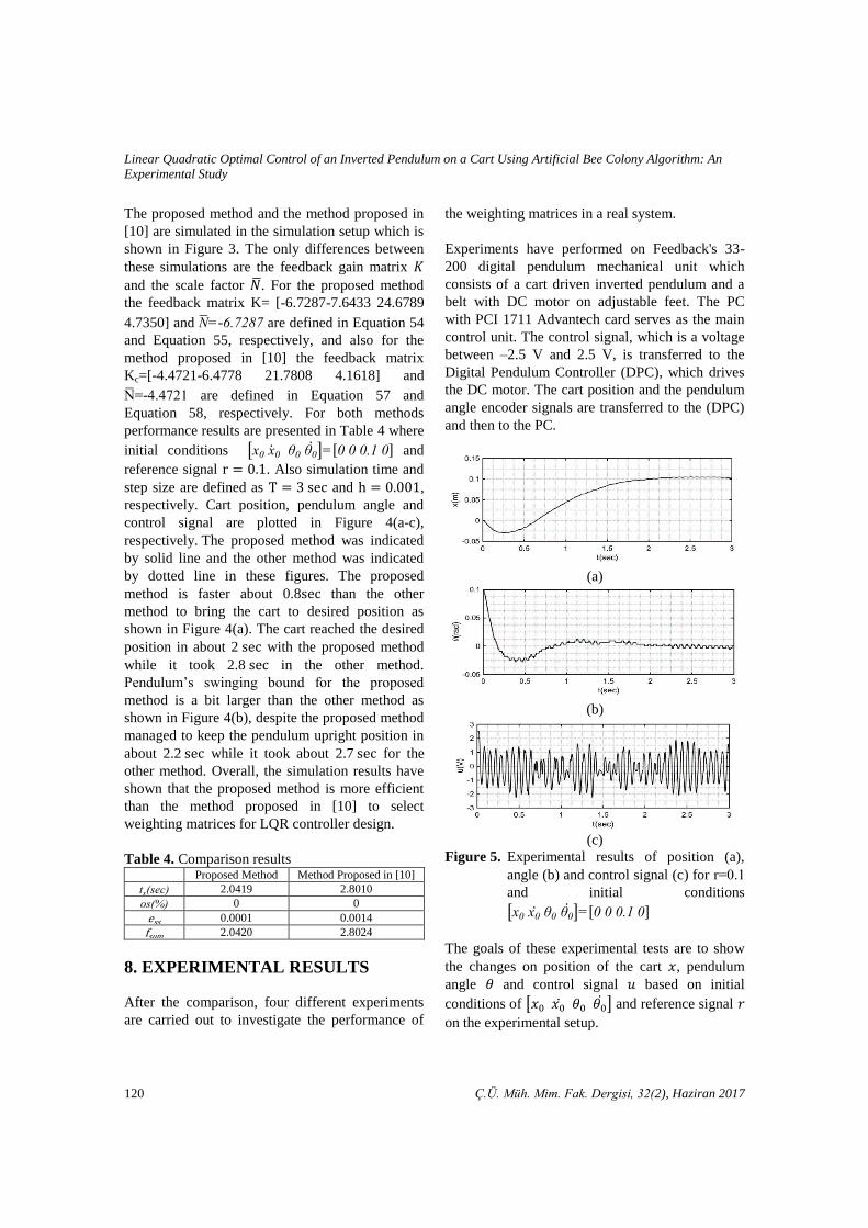
Figure 5. Experimental results of position (a),
angle (b) and control signal (c) for r=0.1
and initial conditions
[x0 x0 θ0 θ0]=[0 0 0.1 0]
The goals of these experimental tests are to show
the changes on position of the cart 𝑥, pendulum
angle 𝜃 and control signal 𝑢 based on initial
conditions of [𝑥0 𝑥0 𝜃0 𝜃0] and reference signal 𝑟
on the experimental setup.

Barış ATA, Ramazan ÇOBAN
Ç.Ü. Müh. Mim. Fak. Dergisi, 32(2), Haziran 2017 121
In the first test, for reference signal 𝑟 = 0.1 and
initial conditions [x0 x0 θ0 θ0]=[0 0 0.1 0], the
cart position (𝑥) , pendulum angle (𝜃) and control
signal (𝑢) are plotted and shown in Figure 5(a-c),
respectively. In the first test, the controller
managed to bring the cart from the initial position
0𝑚 to the desired position in about 2 sec while
bringing the pendulum angle from 0.1 rad to
0 rad as shown in Figure 5(a). Also the pendulum
angle reached to the desired position from the
initial position in about 2 sec as shown in Figure
5(b). The control signal started from 2.5 V and
during the test it was in the range of −2.5 V and
+2.5 V so it obeys physical restriction as shown in
Figure 5(c).
Figure 6. Experimental results of position (a),
angle (b) and control signal (c) for
r = 0.1 and initial conditions
[x0 x0 θ0 θ0]=[0 0 0.2 0]
In the second test, for reference signal r = 0.1 and
initial conditions [x0 x0 θ0 θ0]=[0 0 0.2 0], the
cart position (𝑥), pendulum angle (𝜃) and control
signal (𝑢) are plotted and shown in Figure 6(a-c),
respectively. In the second test, the controller
managed to bring the cart from the initial position
0 m to the desired position in about 2 sec as shown
in Figure 6(a). The pendulum reached to the
upright position from the initial position in about
0.4 sec as shown in Figure 6(b). The control signal
started from 2.5 V and during the test it was in the
range of −2.5 V and +2.5 V as shown in Figure
6(c).
Figure 7. Experimental results of position (a),
angle (b) and control signal (c) for
r = 0.2 and initial conditions
[x0 x0 θ0 θ0]=[0 0 0.1 0]
In the third test, for reference signal r = 0.2 and
initial conditions [x0 x0 θ0 θ0]=[0 0 0.1 0], the
cart position (𝑥), pendulum angle (𝜃) and control
(a)
(b)
(c)
(a)
(b)
(c)
Linear Quadratic Optimal Control of an Inverted Pendulum on a Cart Using Artificial Bee Colony Algorithm: An
Experimental Study
122 Ç.Ü. Müh. Mim. Fak. Dergisi, 32(2), Haziran 2017
signal (𝑢) are plotted and shown in Figure 7(a-c),
respectively. In the third test, the controller
managed to bring the cart from the initial position
0 m to the desired position in about 2.4 sec while
bringing the pendulum angle from 0.1 rad to 0 rad
as shown in Figure 7(a). Also the pendulum angle
reached to the desired position from the initial
position in about 2 sec as shown in Figure 7(b).
The control signal started from 2.5 V and during
the test it was in the range of −2.5 V and +2.5 V
as shown in Figure 7(c).
(a)
(b)
(c)
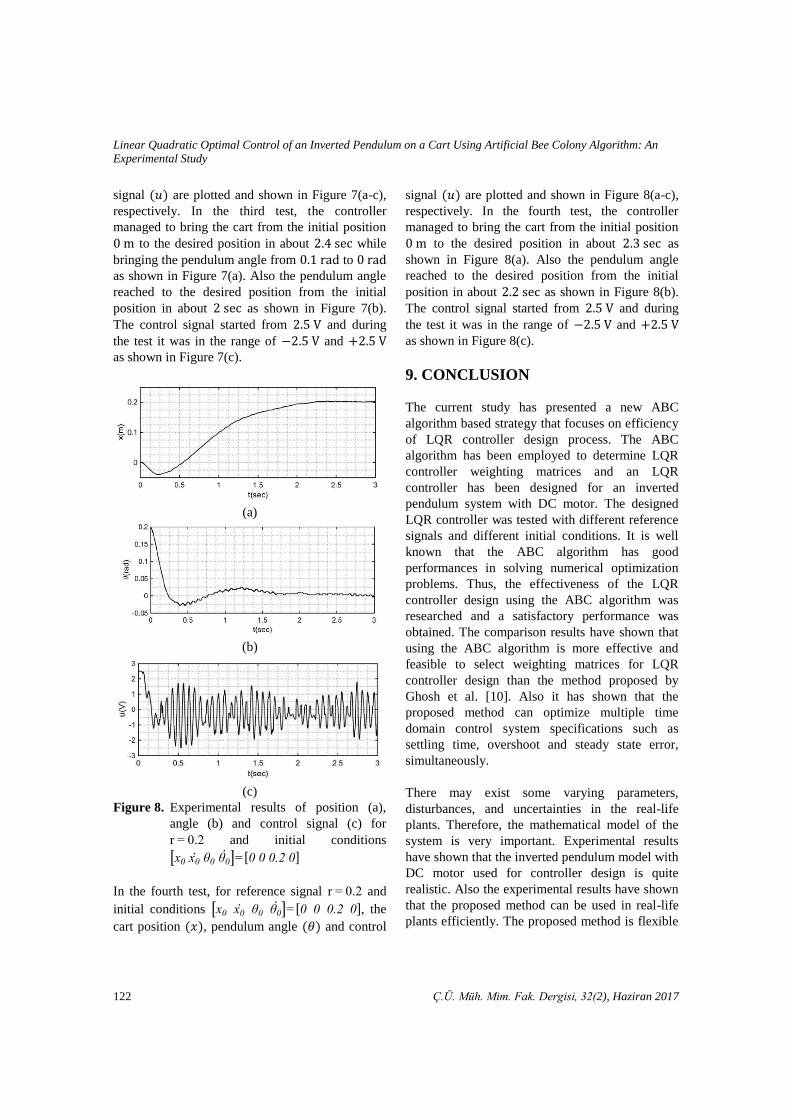
Figure 8. Experimental results of position (a),
angle (b) and control signal (c) for
r = 0.2 and initial conditions
[x0 x0 θ0 θ0]=[0 0 0.2 0]
In the fourth test, for reference signal r = 0.2 and
initial conditions [x0 x0 θ0 θ0]=[0 0 0.2 0], the
cart position (𝑥), pendulum angle (𝜃) and control
signal (𝑢) are plotted and shown in Figure 8(a-c),
respectively. In the fourth test, the controller
managed to bring the cart from the initial position
0 m to the desired position in about 2.3 sec as
shown in Figure 8(a). Also the pendulum angle
reached to the desired position from the initial
position in about 2.2 sec as shown in Figure 8(b).
The control signal started from 2.5 V and during
the test it was in the range of −2.5 V and +2.5 V
as shown in Figure 8(c).
9. CONCLUSION
The current study has presented a new ABC
algorithm based strategy that focuses on efficiency
of LQR controller design process. The ABC
algorithm has been employed to determine LQR
controller weighting matrices and an LQR
controller has been designed for an inverted
pendulum system with DC motor. The designed
LQR controller was tested with different reference
signals and different initial conditions. It is well
known that the ABC algorithm has good
performances in solving numerical optimization
problems. Thus, the effectiveness of the LQR
controller design using the ABC algorithm was
researched and a satisfactory performance was
obtained. The comparison results have shown that
using the ABC algorithm is more effective and
feasible to select weighting matrices for LQR
controller design than the method proposed by
Ghosh et al. [10]. Also it has shown that the
proposed method can optimize multiple time
domain control system specifications such as
settling time, overshoot and steady state error,
simultaneously.
There may exist some varying parameters,
disturbances, and uncertainties in the real-life
plants. Therefore, the mathematical model of the
system is very important. Experimental results
have shown that the inverted pendulum model with
DC motor used for controller design is quite
realistic. Also the experimental results have shown
that the proposed method can be used in real-life
plants efficiently. The proposed method is flexible

Barış ATA, Ramazan ÇOBAN
Ç.Ü. Müh. Mim. Fak. Dergisi, 32(2), Haziran 2017 123
and applicable in a wide range of optimization
problems. Hence, it can be regarded as a general
controller design method that can be applied to a
wide class of control problems.
10. REFERENCES
1. Anderson, C. W., 1989. Learning to Control an
Inverted Pendulum Using Neural Networks,
IEEE Control Systems Magazine, 9(3), 31-37.
2. Kuo, A. D, 2007. The Six Determinants of Gait
and the Inverted Pendulum Analogy: A
Dynamic Walking Perspective, Human
Movement Science, 26(4), 617-656.
3. Jeong, S., Takahashi, T., 2008. Wheeled
Inverted Pendulum Type Assistant Robot:
Design Concept and Mobile Control,
Intelligent Service Robotics, 1(4), 313-320.
4. Feedback Instruments Ltd., 2006. 33-936s
Digital Pendulum Control Experiments
Manual.
5. Kalman, R. E., 1964. When is a Linear Control
System Optimal?, Journal of Basic
Engineering, 86(1), 51-60.
6. Kwakernaak, H., Sivan, R., 1972. Linear
Optimal Control Systems, New York.
7. Fonseca Neto, J.V., Abreu, I. S., Da Silva, F.
N., 2010. Neural–genetic Synthesis for State-
Space Controllers Based on Linear Quadratic
Regulator Design for Eigenstructure
Assignment, IEEE Transactions on Systems,
Man, and Cybernetics, 40(2), 266-285.
8. Yaoqing, W., 1992. The Determination of
Weighting Matrices in lq Optimal Control
Systems, Acta Automatica Sinica, 2(11).
9. Bryson, A. E., 1975. Applied Optimal Control:
Optimization, Estimation and Control, New
York.
10. Ghosh, A., Krishnan, T., Subudhi, B., 2012.
Brief Paper-robust Proportional-integral-
Derivative Compensation of an Inverted Cart-
Pendulum System: An Experimental Study,
IET Control Theory & Applications, 6(8),
1145-1152.
11. Bottura, C. P., Fonseca Neto, J. V., 2000. Rule-
Based Decision-making Unit for Eigenstructure
Assignment Via Parallel Genetic Algorithm
and Lqr Designs, American Control
Conforence Proceedings, 467-471.
12. Mobayen, S., Rabiei, A., Moradi, M.,
Mohammady, B., 2011. Linear Quadratic
Optimal Control System Design using Particle
Swarm Optimization Algorithm, International
Journal of Physical Sciences, 6(30), 6958-
6966.
13. Ata, B., Coban, R., 2015. Artificial Bee Colony
Algorithm Based Linear Quadratic Optimal
Controller Design for a Nonlinear Inverted
Pendulum, International Journal of
International Systems. and Applications in
Engineering, 3(1), 1-6.
14. Karaboga, D., 2005. An Idea Based on Honey
Bee Swarm for Numerical Optimization,
Technical Report TR06, Erciyes University,
Kayseri.
15. Karaboga, D., Basturk, B., 2007. A Powerful
and Efficient Algorithm for Numerical
Function Optimization: Artificial Bee Colony
Algorithm, Journal of Global Optimization,
39(3), 459–471.
16. Ercin, O., Coban, R., 2012. Identification of
Linear Dynamic Systems using Artificial Bee
Colony Algorithm, Turkish Journal of
Electrical Eng. and Computer Sciences, 20(1),
1175–1188.
17. Nise, N. S., 2011. Control Systems
Engineering, USA.
18. Mablekos, V. E., 1980. Electric Machine
Theory for Power Engineers, New York.
19. Ogata, K., 2001. Modern Control Engineering,
New Jersey.
20. Karaboga D., Akay, B., 2009. A Comparative
Study of Artificial Bee Colony Algorithm,
Applied Mathematics and Computation,
214(1), 108–132.
21. Coban, R., 2011. A fuzzy Controller Design for
Nuclear Research Reactors using the Particle
Swarm Optimization Algorithm, Nuclear Eng.
and Design, 241(5), 1899–1908.
22. Messner, W., Tilbury, D., Inverted Pendulum:
State-space Methods for Controller Design,
http://ctms.engin.umich.edu/CTMS/index.php?
example=InvertedPendulum§ion=ControlS
tateSpace , Accessed:02:12:2016.
23. Franklin, G. F., 1997. Powell, D. J., Workman,
M. L., Digital Control of Dynamic Systems.
UK.
24. Ayres, F., 1976. Matrices, New York.

Linear Quadratic Optimal Control of an Inverted Pendulum on a Cart Using Artificial Bee Colony Algorithm: An
Experimental Study
124 Ç.Ü. Müh. Mim. Fak. Dergisi, 32(2), Haziran 2017