Simulation of the inverted pendulum

Interdisciplinary Project inComputer Science and Mathematics

Christian Wachinger Michael PockComputer Science Computer Science

Project Supervisor:Prof. Dr. Peter Rentrop

TU Munchen

17.12.2004

1

CONTENTS CONTENTS

Contents

1 Task of the interdisciplinary project 4

2 Mechanical model 5

2.1 General problem . . . . . . . . . . . . . . . . . . . . . . . . . . . . . . . . . . . . 5

2.2 Inverted one-bar pendulum . . . . . . . . . . . . . . . . . . . . . . . . . . . . . . 5

2.3 Inverted n-bar pendulum . . . . . . . . . . . . . . . . . . . . . . . . . . . . . . . 7

3 Simulation systems 9

3.1 One-step solver . . . . . . . . . . . . . . . . . . . . . . . . . . . . . . . . . . . . . 9

3.2 Explicit Euler . . . . . . . . . . . . . . . . . . . . . . . . . . . . . . . . . . . . . . 10

3.3 Runge-Kutta methods . . . . . . . . . . . . . . . . . . . . . . . . . . . . . . . . . 11

3.4 Step size control . . . . . . . . . . . . . . . . . . . . . . . . . . . . . . . . . . . . 11

3.5 Dormand-Prince method . . . . . . . . . . . . . . . . . . . . . . . . . . . . . . . . 12

4 Controller design 13

4.1 Basics of controller design . . . . . . . . . . . . . . . . . . . . . . . . . . . . . . . 13

4.2 Controlling with pole location presetting . . . . . . . . . . . . . . . . . . . . . . . 15

4.3 Controller design for the inverted pendulum . . . . . . . . . . . . . . . . . . . . . 16

5 Neural network 18

5.1 Basics of neural networks . . . . . . . . . . . . . . . . . . . . . . . . . . . . . . . 18

5.2 Feed-forward networks . . . . . . . . . . . . . . . . . . . . . . . . . . . . . . . . . 18

5.3 Learning through backpropagation . . . . . . . . . . . . . . . . . . . . . . . . . . 19

5.4 Reinforcement networks . . . . . . . . . . . . . . . . . . . . . . . . . . . . . . . . 20

6 Simulation results 24

6.1 One-bar Pendulum . . . . . . . . . . . . . . . . . . . . . . . . . . . . . . . . . . . 24

6.2 Double pendulum . . . . . . . . . . . . . . . . . . . . . . . . . . . . . . . . . . . . 30

7 Conclusions 30

2

CONTENTS CONTENTS

3

1 TASK OF THE INTERDISCIPLINARY PROJECT

Abstract

In this paper, the problem of the inverted n-bar pendulum in the plane is discussed. Thedescriptor form and the state space form, which corresponds to an ordinary differential equa-tion system (ODE), are deduced. The simulating systems for solving the ODE are describedand controllers for the one-bar and the two-bar case are developped. Also, a neural networkfor the task of controlling the inverted pendulum was trained.

1 Task of the interdisciplinary project

The project was done by two computer science students and the project was supervised byProfessor Rentrop, chair of numerical mathematics at TU Munchen. The task was split up intothree parts:

1. We had to model the inverse n-bar pendulum in the plane with the help of the descriptorand state space form. The descriptor form bases on redundant coordinates and results in adifferential algebraic equation of index 3. It is possible to solve the constraints explicitly asthe inverse n-bar pendulum has a tree structure. This is the transfer from the descriptorto the state space form which is characterised by a minimal set of local coordinates. Thestate space form is a system of ordinary differential equations.The pendulum should be simulated with the help of the mathematical development envi-ronment Matlab.

2. The modelled system should be controlled by a classical PD-controller, which can bededuced from the pendulum equations. With help of this controller a neural networkshould be developed, which can also regulate the inverted pendulum.

3. The simulation of the pendulum should be visualized with the help of the graphical toolsin Matlab.

4

2 MECHANICAL MODEL

2 Mechanical model

2.1 General problem

The problem we have to deal with can be described with the help of the equations of motion,which lead to a large system of differential algebraic equations. [3] These are the Lagrangeequations of the first kind, which are in descriptor form. They describe a mechanical systemof bodies with massless connections. The equations of motion according to Newton withoutconstraints are

p = v

M(p, t)v = f(p, v, t) (1)

with p ∈ R the vector of position coordinates, v ∈ Rn the vector of the velocity coordinates,M(p, t) ∈ Rn,n the symmetric and positive definite mass matrix and f(p, v, t) ∈ Rn the vectorfor the applied external forces. The connections cause the following constraints which are alsodenoted as the geometry of the system

0 = b(p, t), b(p, t) ∈ Rq.

By using Lagrange multipliers λ(t) ∈ Rq, equation (1) can be transformed to the descriptor form

p = v

M(p, t)v = f(p, v, λ, t)− (∂

∂p)b(p, t))T λ (2)

0 = b(p, t).

The equation (2) is a differential-algebraic system (DAE) of index three. In the following sectionswe will apply these equations to the inverted pendulum problem. So far it is not possible to derivea controller directly from the descriptor form, so it is necessary to transfer them into the statespace form. It corresponds to an ordinary differential equation system (ODE)

M(p, t)¨p = f(p, v, t) (3)

System (3) is also known as the Lagrange equations of the second kind.

2.2 Inverted one-bar pendulum

In this part we will concentrate on modelling an inverted one-bar pendulum. The model of themechanical system of this pendulum can be seen in figure 1. It consists of a cart with mass mconcentrated in the joint and one bar with length 2l1 and mass m1 concentrated in its centre.The car can move in horizontal direction. The inertia I1 is under the influence of the gravity.Coordinates p are:

• the position x of the cart

• the position x1, y1 of the bar centre

• the angle ϕ1.

Introducing constraint forces Fz1, · · · , Fz4 the Newton-Euler formulation gives

5

2.2 Inverted one-bar pendulum 2 MECHANICAL MODEL

Figure 1: Cart with inverted one-bar pendulum

mx = F + Fz1

m1x1 = Fz2

m1y1 = −m1g + Fz3

I1ϕ1 = Fz4

0 = x− x1 + l1sin(ϕ1)0 = y1 − l1cos(ϕ1)

The last two equations describe the geometry

b(p) = b(x, x1, y1, ϕ1) = 0

of the system. The inertia of a bar with length 2l1 is according to Steiner

I1 =43m1l

21.

With the help of D’Alembert, see [3], we get the descriptor form:

mx = F + λ1

m1x1 = −λ1

m1y1 = −m1g − λ2 (4)I1ϕ1 = λ1l1cosϕ1 − λ2l1sinϕ1

0 = x− x1 + l1sin(ϕ1)0 = y1 − l1cos(ϕ1)

6

2.3 Inverted n-bar pendulum 2 MECHANICAL MODEL

The state space form can be deduced from (4) by solving for x and ϕ1.(m + m1 m1l1cosϕ1

m1l1cosϕ1 I1 + m1l21

) (x

ϕ1

)=

(F + m1l1sinϕ1ϕ1

2

m1l1sinϕ1g

)(5)

(5) is a classical state space formulation consisting of two second order ODEs with a symmetricmass-matrix.

2.3 Inverted n-bar pendulum

Figure 2: Cart with inverted n-bar pendulum

The layout of the cart with the n-bars can be seen in the figure 2. The equations of motioncan be written analogously to the one-bar problem. The state space form is listed below, thededuction can be seen in [3]. We define:

cji := cji(ϕ) = cos(ϕj − ϕi), sji := sji(ϕ) = sin(ϕj − ϕi)

mi =n∑

k=i+1

mk, i, j = 1, · · · , n

The following matrix M is symmetric:

7

3 SIMULATION SYSTEMS

M =

m + m0 (m1 + 2m1)l1 cos ϕ1 · · · (mj + 2mj)lj cos ϕj · · · · · · · · · mnln cos ϕn

· · · I1 + (m1 + 4m1)l21 · · · 2(mj + 2mj)lilj · · · · · · · · · 2mnl1lncn1

......

......

......

......

· · · · · · · · · Ii + (mi + 4mi)l2i · · · 2(mj + 2mj)liljcji · · · 2mnlilncni

......

......

......

......

· · · · · · · · · · · · · · · · · · · · · In + mnl2n

B =

F(m1 + 2m1)gl1 sinϕ1

...(mi + 2mi)gli sinϕi

...mngln sinϕn

+

(m1 + 2m1)l1 sinϕ1

2(m1 + 2m1)l21s11

...2(mi + 2mi)l1lis1i

...2mnl1lns1n

ϕ2

1 + · · ·+

(mj + 2mj)lj sinϕj

2(mj + 2m1)lj l1sj1

...2(mj + 2mi)lj lisji

...2mnlj lnsjn

ϕ2

j +

+ · · ·+

mnln sinϕn

2mnl1lnsn1

...2mnlilnsni

...2mnl2nsnn

ϕ2

n

The general compact state space form is:

M

xϕ1

...ϕi

...ϕn

= B (6)

3 Simulation systems

For the simulation of the inverted pendulum problem, we have used the mathematical devel-opment environment Matlab. Matlab was chosen, as it is widely used in the field of numericalmathematics and supports solving ordinary differential equations. Moreover, it is possible to vi-sualize the simulation results. In our program we used the ode45, a standard solver included inMatlab, to solve the ordinary differential equation (ODE). The ode45 implements the method ofDormand-Prince, which is a member of the class of Runge-Kutta-Fehlberg methods. The reasonwhy we need such a solver is that it is not possible to solve the ODE analytically.

8

3.1 One-step solver 3 SIMULATION SYSTEMS

3.1 One-step solver

For solving an initial value problem

y′ = f(x, y), y(x0) = y0 (7)

a numerical method is needed. One step solver are defined by a function Φ(x, y, h; f) which givesapproximated values yi := y(xi) for the exact solution y(x):

yi+1 := yi + hΦ(xi, yi, h; f)xi+1 := xi + h

where h denotes the step size. In the following be x and y arbitrary but fixed, and z(t) is theexact solution of the initial value problem

z′(t) = f(t, z(t)), z(x) = y

with the initial values x and y. Then the function

∆(x, y, h; f) :={

z(x+h)−yh h 6= 0

f(x, y) h = 0

describes the differential quotient of the exact solution z(t) with step size h, whereas Φ(x, y, h; f)is the differential quotient of the approximated solution with step size h.The difference τ = ∆−Φ is the measure of quality of the approximation method and is denotedas local discretisation error.

In the following, FN (a, b) is defined as the set of all functions f , for which exist all partialderivations of order N on the area

S = {x, y|a ≤ x ≤ b, y ∈ Rn}, a,b finite,

where they are continuous and limited.

One step solvers have to fulfill

limh→0

τ(x, y, h; f) = 0.

This is equivalent to

limh→0

Φ(x, y, h; f) = f(x, y).

If this condition holds for all x ∈ [a, b], y ∈ F1(a, b), then Φ and the corresponding one stepmethod are called consistent.

The one step method is of order p, if

τ(x, y, h; f) = O(hp)

holds for all x ∈ [a, b], y ∈ R, f ∈ Fp(a, b).

The global discretisation error

9

3.2 Explicit Euler 3 SIMULATION SYSTEMS

en(X) := y(X)− yn X = xn fix , n variable

is the difference between exact solution and the approximated solution.

The one step method is denoted as convergent, if:

limn→∞

‖en(X)‖ = 0.

Theorem: Methods of order p > 0 are convergent and it holds

en(X) = O(hp).

This means that the order of the global discretisation error is equal to the order of the localdiscretisation error.

The crucial problem concerning one step methods is the choice of the step size h. If thestep size is too small, the computational effort of the method is unnecessary high, but if thestep size is too large, the global discretisation error increases. For initial values x0, y0 a step sizeas large as possible would be chosen,so that the global discretisation error is below a boundaryε after each step. Therefore a step size control is necessary.

3.2 Explicit Euler

The most elementar method of solving initial value problems is the explicit Euler. The value ofyi+1 can be calculated the following way:

yi+1 = yi + h · f(xi, yi) (8)

The explicit Euler calculates the new value yi+1 by following the tangent at the old value yi fora distance of h. The slope of the tagent is given by the value of f(xi, yi). The explicit Euler uses

Figure 3: Explicit Euler

no step size control, the step size h is fix. So it is only useful in special cases, where the functionto integrate is pretty flat. But it is very easy to implement and calculates very fast, so it can bea good choice.

10

3.3 Runge-Kutta methods 3 SIMULATION SYSTEMS

3.3 Runge-Kutta methods

The Runge-Kutta methods are a special kind of one step solvers, which evaluate the right sidein each step several times. The intermediate results are combined linearly.The general discretisation schema for one step of a Runge-Kutta method is

y1 = y0 + h(b1K1 + b2K2 + · · ·+ bsKs)

with corrections

Ki = f(x0 + cih, y0 + hi−1∑j=1

aijKj), i = 1, · · · , s.

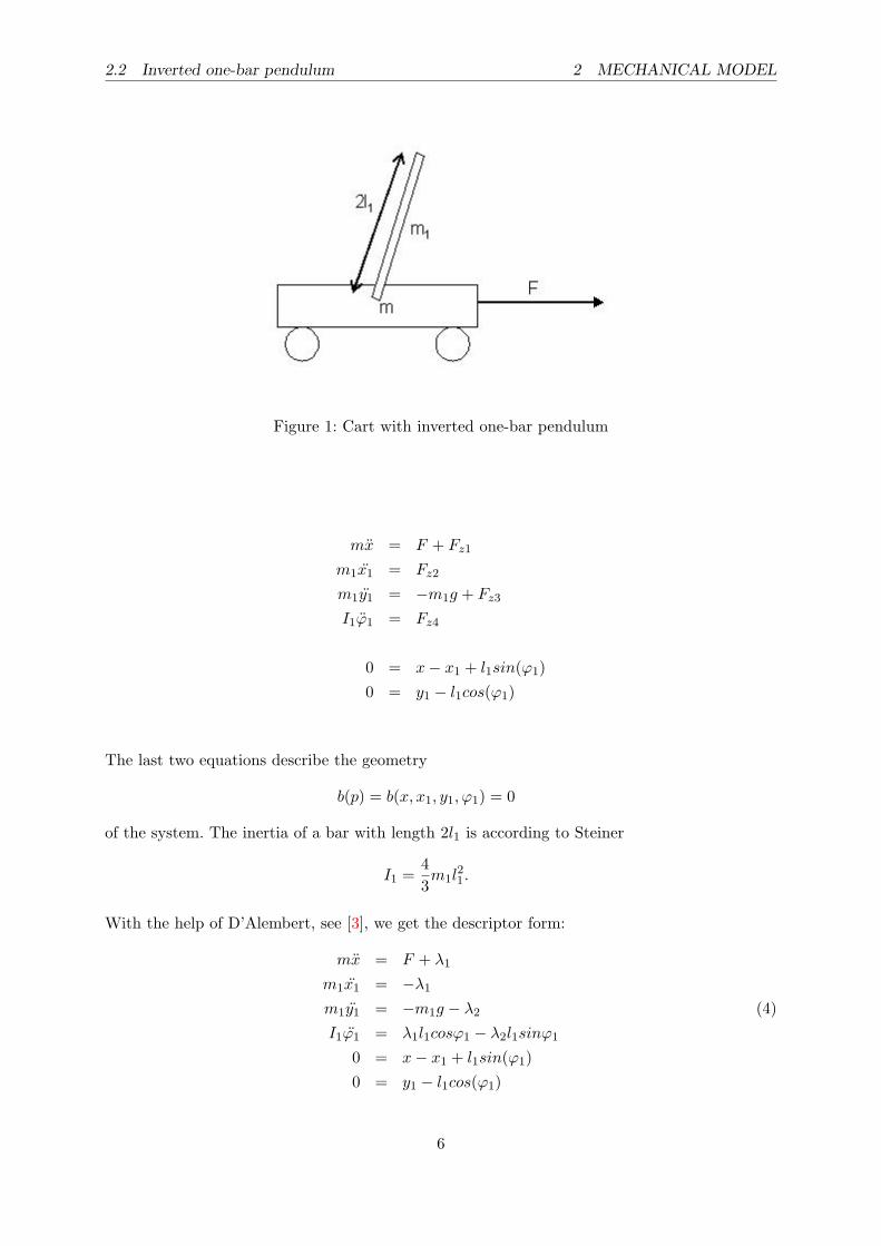
The coefficients are summarized in a tableau, the so called Butcher-tableau, see figure 4.

Figure 4: Butchertableau

3.4 Step size control

The Runge-Kutta methods use an equidistant grid, but this is for most applications inefficient.A better solution is to use an adaptive step size control. The grid has to be chosen so that

• a given accuracy of the numerical solution is reached

• the needed computational effort is minimized.

As the characteristics of the solution are a priori unknown, a good grid structure can not bechosen previous to the numerical integration. Instead, the grid points have to be adapted duringthe computation of the solution.Trying to apply this to Runge-Kutta methods lead to the following technique:To create a method of order p (for yi+1), it is combined with a method of order p+1 (for yk+1).This method for yi+1 is called the embedded method. The idea of embedding was developed byFehlberg and methods using this technique therefore are called Runge-Kutta-Fehlberg methods.This leads to a modified Butchertableau. (see figure 5)

The new step size is calculated with

hnew = h p+1

√ε

‖y − y‖

where ε denotes the tolerance.

11

3.5 Dormand-Prince method 4 CONTROLLER DESIGN

Figure 5: Modified Butchertableau for embedded Runge-Kutta-methods

3.5 Dormand-Prince method

The Dormand-Prince method is a member of the Runge-Kutta-Fehlberg class with order 4(5).It means that the method has order 5 and the embedded method has order 4. This is describedby the following equations:

y(x0 + h) = y0 + h4∑

k=0

bkfk(x0, y0;h)

y(x0 + h) = y0 + h

5∑k=0

bkfk(x0, y0;h)

fk = f(x0 + ckh, y0 + h

k−1∑t=0

aklfl)

In Matlab this ODE solver is implemented in the function ode45. The coefficients from Dormandand Prince can be seen in figure 6.

4 Controller design

4.1 Basics of controller design

There are several basic requirements to a controller:

• Stability

• Stationary accuracy

• Promptness

The basic principle for the control of a system is a complete description of the system byequations. For these inverted pendulum problem the equations are stated in section 2.A linear dynamic system is described by

12

4.1 Basics of controller design 4 CONTROLLER DESIGN

Figure 6: Butchertableau for Dormand-Prince-method

Figure 7: Schema of the functionality of the controller

x(t) = Ax(t) + Bu(t) (9)y(t) = Cx(t) + Du(t)

with A,B, C, D ∈ Rn,n constant. Assuming that there is no disturbance, the vector u(t) repre-sents the control variables. The vector y(t) denotes the measurement values. For the invertedpendulum problem, this means, that C is the unity matrix I and D is zero. The initial statex0 = x(t0) is in general unknown. There are several characteristics of a controller:

Controllability: The system (9) is called controllable, if the state space vector x can be movedto the finite state 0 within a finite time frame and an arbitrary initial state x0 by the correctchoice of the variable control vector u. The finite state 0 is not a limitation, as the coordinatesystem can be translated to the appropriate values.

13

4.1 Basics of controller design 4 CONTROLLER DESIGN

Observability: The system (9) is called observable, if the initial state x0 can be uniquelycalculated with a known u(t) and the measurement of y(t).

Stability: The system (9) is called stable if the solution x(t) of the homogeneous state spacedifferential equation x = Ax tends to 0 for t →∞. This holds for any initial state x0.

A linear system hast to be controllable and observable, so that it can be controlled. Thestability of the control path is necessary, as otherwise one of the basic requirements is notfulfilled.There are two different possibilities for the design of a controller. It can be designed in statespace or in frequency domain. In the following we will concentrate on the development in statespace where the linear system (9) can be handled with the KALMAN-criteria:

• The system (9) with u ∈ Rp is controllable if and only if the n× np controllability matrix

QS = (B,AB,A2B, · · · , An−1B)

has maximum rank n.

14

4.2 Controlling with pole location presetting 4 CONTROLLER DESIGN

• The system (9) with y ∈ Rq is observable if and only if the nq×n observability matrix QBC

CA...

CAn−1

has maximum rank n.

For the caracterisation of the stability, there exists the following theorem:

Theorem: The system (9) is stable if and only if all eigenvalues of A have a negative real part.

4.2 Controlling with pole location presetting

In the following a controller is designed by pole location presetting. This is done by presettingthe eigenvalues λ1, · · · , λn of the state space control to ensure that the controller r has theseeigenvalues. This leads to:

det(sI − (A− brT )) =n∏

ν=1

(s− λν) = sn + pn−1sn−1 + · · ·+ p1s + p0

=⇒ sn + an−1(r)sn−1 + · · ·+ a0(r) = sn + pn−1sn−1 + · · ·+ p1s + p0

r can be calculated by a comparison of the coefficients. But this approach has the disadvantage,that the effort of the evaluation of the determinante is too high and therefore the formula ofAckerman is used.

Theorem of Ackermann: If the control path x = Ax+ bu is controllable and the state spacecontrol has the characteristic polynomial p(s) = sn +an−1s

n−1 + · · ·+a1s+a0, then the controlvector is chosen as

rT = p0tT1 + p1t

T1 A+ · · ·+ pn−1t

T1 An−1 + tT1 An = tT1 [p0I + p1A+ · · ·+ pn−1A

n−1 +An] = tT1 p(A).

with tT1 as the last row of the inverse controllability matrix Q−1S and it is calculated by the

system of equations

tT1 b = 0tT1 Ab = 0

...tT1 An−2b = 0tT1 An−1b = 1

15

4.3 Controller design for the inverted pendulum 4 CONTROLLER DESIGN

4.3 Controller design for the inverted pendulum

In this section, the theory of control design of the last section shall be applied to the invertedpendulum problem. There are many articles concerning the problem of broomstick balancing, e.g.K. Furuta, [4] who approached the problem from a technical point of view and P. J. Larcombe,[5] who focused on the mathematical point of view.The inherent dificulty of controlling the inverted pendulum is, that is not a linear system.Unfortunately, there are only linear controllers, which cannot control non-linear systems. Butas the inverted pendulum behaves nearly linear, while it is balanced, it is possible to linearisethe equations of the pendulum for small angles. So the linear controlling theory can be applied.

4.3.1 Inverse one-bar pendulum

To develop a controller, the equation (5) has to solved for x and ϕ1 and linearised by settingcos(ϕ1) = 1, sin(ϕ1) = ϕ1 and ϕ1

2 = 0 for small ϕ1:

x = − 3m1g

4m1 + 7m· ϕ1 +

74m1 + 7m

· F

ϕ1 = − 3(m + m1)gl(4m1 + 7m)

· ϕ1 −3

l(4m1 + 7m)· F

By setting the state variables x1 := x, x2 := x, x3 := ϕ1, x4 := ϕ1 (xT = (x1, · · · , x4)) and theinput value u := F the control system is:

x =

0 1 0 00 0 − 3m1g

4m1+7m 00 0 0 10 0 3(m+m1)g

l(4m1+7m) 0

x +

07

4m1+7m

0− 3

l(4m1+7m)

u =: Ax + bu

The control path is controllable as the determinate of the controllability matrix

QS = (B,AB,A2B, · · · , An−1B)

is not zero. Moreover it is observable as the observability matrix QBC

CA...

CAn−1

has maximum rank 4, see [6]. Therefore the first two criteria are fulfilled and to fulfill also thethird criteria, the stability, all the eigenvalues of A must have a negative real part. This is nottrue as the eigenvalues are:

s1/2 = 0, s3/4 = ±

√3(m + m1)gl(4m1 + 7m)

Applying all these steps to the inverted pendulum problem we get the following results:

tT1 = [l(4m1 + 7m)

3g, 0,

7l2(4m1 + 7m)9g

, 0]

16

4.3 Controller design for the inverted pendulum 4 CONTROLLER DESIGN

leading to

r1 = −p0 ·l(4m1 + 7m)

3g

r2 = −p1 ·l(4m1 + 7m)

3g

r3 = −p0 ·7l2(4m1 + 7m)

9g− p2 ·

l(4m1 + 7m)3g

− (m + m1)g

r4 = −p1 ·7l2(4m1 + 7m)

9g− p3 ·

l(4m1 + 7m)3g

In the next step the variables p0, · · · , p3 have to be calculated. This works with the Theorem ofAckermann. Denoting the eigenvalues as λ1, · · · , λ4, this leads to

p(s) = (s− λ1)(s− λ2)(s− λ3)(s− λ4) = s4 + p3s3 + p2s

2 + p1s + p0 (10)

By using the quad eigenvalue λ = −1 the coefficients pi are

p0 = 1, p1 = 4, p2 = 6, p3 = 4.

Eventually the force F which controls the system is made up of

F = −r1x− r2x− r3ϕ− r4ϕ.

4.3.2 Inverted double pendulum

In this section a controller for the inverted double pendulum shall be developed. An approach likein the one-bar case is chosen. First of all the state space form of the double pendulum problemis linearised to reduce the complexity of the system. This is achieved by setting cos(ϕi) = 1,sin(ϕi) = ϕi and ϕ2

i = ϕ22 = 0 for small ϕi with i = 1,2. Moreover it is assumed that m1 = m2

and l1 = l2. Concerning this and solving for x, ϕ1 and ϕ2 leads to xϕ1

ϕ2

= 3l1(56m1+97m

l1 · (973 F − 45m1ϕ1g −m1ϕ2g)

3 · (−5F + (7m + 11m1)ϕ1g − (2m + m1)ϕ2g)−F − 9(2m + m1)ϕ1g + (19m + 11m1)ϕ2g

Similar to the one-bar pendulum the state variables are set to x1 := x, x2 := x, x3 := ϕ1,x4 := ϕ1, x5 := ϕ2, x6 := ϕ2 (xT = (x1, · · · , x6)) and the input value u := F . This leads to thecontrol system:

x =

0 1 0 0 0 00 0 − 135m1g

56m1+97m 0 − 135m1g56m1+97m 0

0 0 0 1 0 00 0 9(7m+11m1)g

l1(56m1+97m) 0 − 9(2m+m1)gl1(56m1+97m) 0

0 0 0 0 0 10 0 27(2m+m1)g

l1(56m1+97m) 0 −3(19m+11m1)gl1(56m1+97m) 0

x +

097

56m1+97m

0− 45

l1(56m1+97m)

0− 3

l1(56m1+97m)

u =: Ax + bu

17

5 NEURAL NETWORK

The control path is also controllable and observable, as the determinants of the controllabilitymatrix QS and the observability matrix QB are not zero. But like in the one-bar case it is notstable.The Theorem of Ackermann is applied to the system and we receive the vector t1, with whichthe controller can be developed. A sixfold eigenvalue λ = −3 is used and the coefficients pi are:

p0 = 729, p1 = 1458, p2 = 1215, p3 = 540, p4 = 135, p5 = 18.

The force F is set to

F = −r1x− r2x− r3ϕ1 − r4ϕ1 − r5ϕ2 − r6ϕ2.

5 Neural network

In this section an approach to control the inverted pendulum by using neural networks is de-scribed. Neural networks are modelled similar to the human brain. They are often used to solvehard problems, where it is difficult to write exact algorithms, or where the exact algorithms areto slow.

5.1 Basics of neural networks

The aim of neural networks is to simulate a function. But before the function can be simulated,the network has to learn its behaviour. For this purpose exist several learning algorithms. Whatkind of functions the network is able to simulate, depends on its topology.

A neural network consists of a set of so called neurons and connections inbetween, the so calledsynapses. The neural network can also be seen as a graph G = (V,E) where the nodes of thegraph V are the neurons and the edges of the graph G are the synapses. Each synapse (i, j) ∈ Ehas a certain weight wji ∈ R.

5.2 Feed-forward networks

A special kind of neural networks are the feed-forward networks (figure 8). The neurons of thisnetworks are allocated of several disjunct layers, where the first layer is the input layer andthe last one is the output layer. Layers between the first and last layer are the so called hiddenlayers. There are no connections between neurons of the same layer. The information flows justin one direction from the input to the output layer.How many layers are used in a neural network depends on the problem. By changing the numberof layers in a network, the separation possibility of it changes. With a one-layered network linearseparation can be achieved. With a two layered network convex areas can be separated.The activation of a neuron ok in layer r can be computed as

netk =∑

l ∈ layer < r wklol, ok = f(netk)

with an activation function f. The activation function should be non-linear. One frequently usedfunction is the logistic function

18

5.3 Learning through backpropagation 5 NEURAL NETWORK

Figure 8: Two-layered feed-forward network

f(x) = 11+e−x

with the derivation

f ′(x) = f(x)(1− f(x)).

5.3 Learning through backpropagation

The most frequently used learning algorithm for both supervised and reinforcement learning isthe backpropagation algorithm.In the first part a simple forward propagation is used to evaluate the network and to determinethe output error

E = 12

∑i in output layer(oi − di)2

with the desired output di of the i-th output node. In the next part a technique called gradientdescent is used to change the weights

wij := wij + ∆wij = wij − α ∂E∂wij

with the learn rate α. The gradient is

19

5.4 Reinforcement networks 5 NEURAL NETWORK

− ∂E∂wij

= − ∂E∂oi

∂oi∂neti

∂neti∂wij

= δioj

with

δi = − ∂E∂neti

= − ∂E∂oi

f ′(neti).

If i is an output node then

∂E∂oi

= (oi − di).

Otherwise if i is not an output node and in the r-th layer then by using the chain rule

∂E∂oi

=∑

k ∈ layer > r∂E

∂netk∂netk∂oi

=∑

k ∈ layer > r δkwki.

Now an error propagation algorithm is used which is symmetric to the forward propagationalgorithm:

netk =∑

l ∈ layer < r wklf(netl).

When using the error propagation algorithm, first of all the error (di − oi)f ′(neti) must beassigned to the output nodes. Then the error is backpropagated through the network

δi = f ′(neti)∑

k ∈ layer > r wkiδk.

This means, that the error of one node is calculated by summing up the errors of all successivenodes, multiplying each error with the corresponding weight and multiplying this sum with theactivation of the node applied to the derivation of f. Eventually all the weights of the networkare changed

wij := wij + αδioj .

Like stated above a gradient descent method is used within the backpropagation algorithm. Theproblem of this method is, that it can get stuck in local minimum and therefore, the globalminimum can not be found. It depends on the initial choice of the weights, which minimum isfound. This means that with a good choice of the initial weights, within some training steps,a good minimum can be found, whereas otherwise, if there is a bad initial set of weights, evenafter a lot of time spent in training of the network, it will not work properly.

5.4 Reinforcement networks

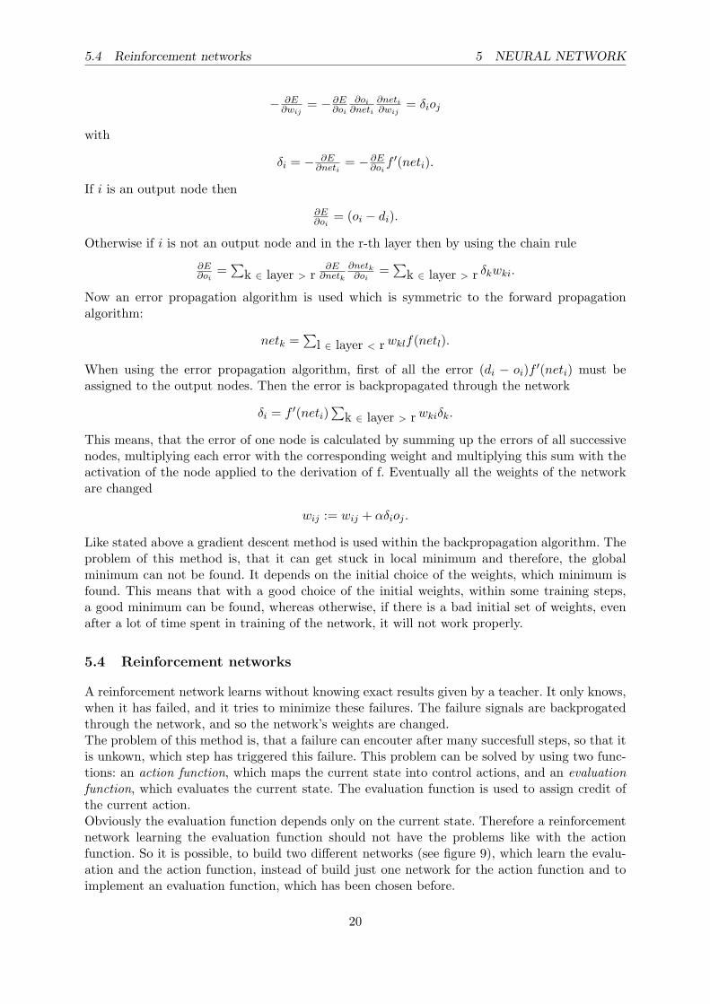
A reinforcement network learns without knowing exact results given by a teacher. It only knows,when it has failed, and it tries to minimize these failures. The failure signals are backprogatedthrough the network, and so the network’s weights are changed.The problem of this method is, that a failure can encouter after many succesfull steps, so that itis unkown, which step has triggered this failure. This problem can be solved by using two func-tions: an action function, which maps the current state into control actions, and an evaluationfunction, which evaluates the current state. The evaluation function is used to assign credit ofthe current action.Obviously the evaluation function depends only on the current state. Therefore a reinforcementnetwork learning the evaluation function should not have the problems like with the actionfunction. So it is possible, to build two different networks (see figure 9), which learn the evalu-ation and the action function, instead of build just one network for the action function and toimplement an evaluation function, which has been chosen before.

20

5.4 Reinforcement networks 5 NEURAL NETWORK

5.4.1 Controlling the inverted pendulum with a reinforcement network

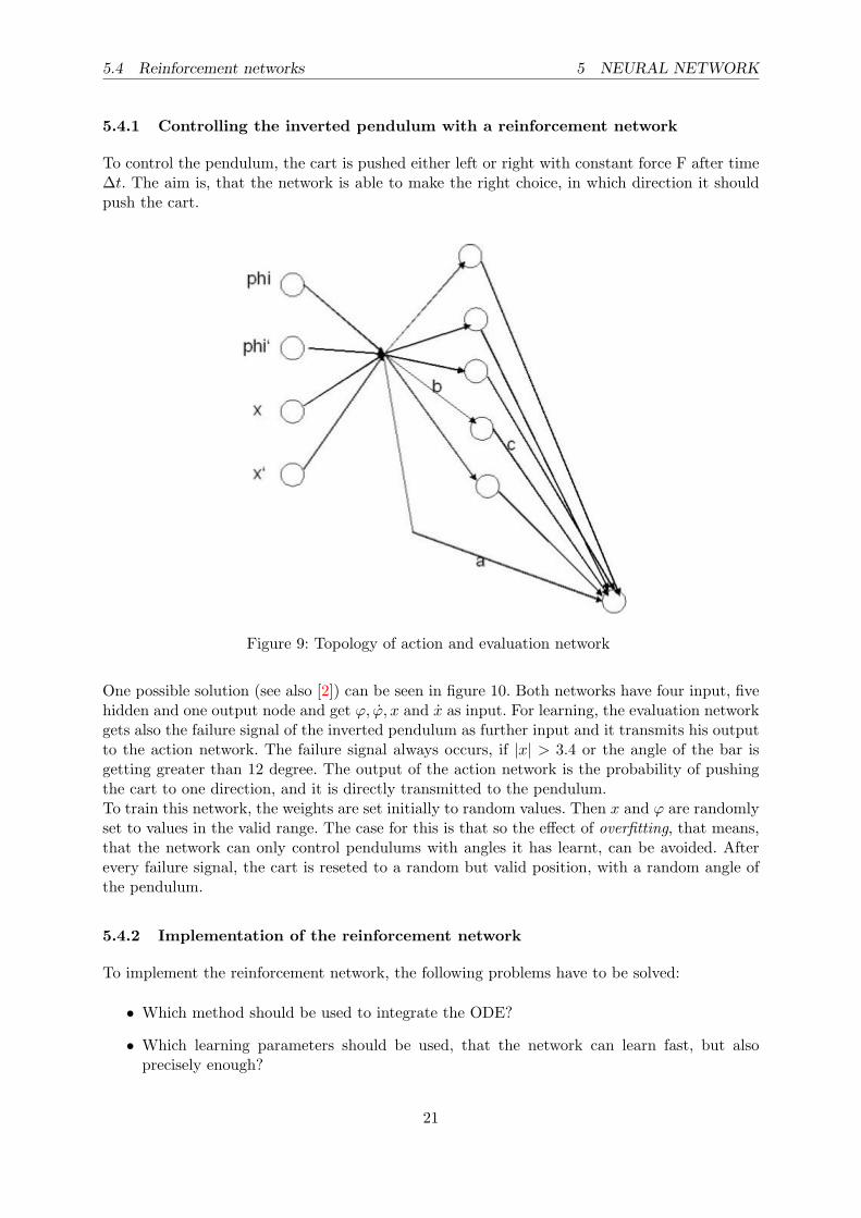
To control the pendulum, the cart is pushed either left or right with constant force F after time∆t. The aim is, that the network is able to make the right choice, in which direction it shouldpush the cart.

Figure 9: Topology of action and evaluation network

One possible solution (see also [2]) can be seen in figure 10. Both networks have four input, fivehidden and one output node and get ϕ, ϕ, x and x as input. For learning, the evaluation networkgets also the failure signal of the inverted pendulum as further input and it transmits his outputto the action network. The failure signal always occurs, if |x| > 3.4 or the angle of the bar isgetting greater than 12 degree. The output of the action network is the probability of pushingthe cart to one direction, and it is directly transmitted to the pendulum.To train this network, the weights are set initially to random values. Then x and ϕ are randomlyset to values in the valid range. The case for this is that so the effect of overfitting, that means,that the network can only control pendulums with angles it has learnt, can be avoided. Afterevery failure signal, the cart is reseted to a random but valid position, with a random angle ofthe pendulum.

5.4.2 Implementation of the reinforcement network

To implement the reinforcement network, the following problems have to be solved:

• Which method should be used to integrate the ODE?

• Which learning parameters should be used, that the network can learn fast, but alsoprecisely enough?

21

5.4 Reinforcement networks 5 NEURAL NETWORK

As we have an equidistant timegrid, it is not possible to use the Dormand-Prince-method or theother in Matlab implemented integrators. So it is necessary to use a much simpler method.The most simple integration-method is the explicit Euler. For a fine grid and functions withsmall derivations, it integrates the function fast and precisly. But it does not work well with arough grid or functions with large derivations, as it becomes very unprecisly.But dealing with the inverted pendulum, this problems can be avoided. The grid can be chosensmall enough, and as the calculation is breaked, if there are to large values, our function, whichis integrated, is pretty flat. So it is a good choice, as it works very well for this case and it isalso very easy to implement.The right choice of the learning parameters is much harder. We have succesfully used the fol-lowing ones (see [1]):

γ = 0.9βe = 0.2βa = 0.2ρe = 1ρa = 0.05

Be t the current time. Define the input vector v as follow:

v =

x+2,4

4,8x+1,5

3ϕ+0,2094

0,4186ϕ+2,01

4,02

0, 5

Define the following activation functions:

• yte for the hidden layer in the evaluation network e at time t

• zte for the output node in the evaluation network e at time t

• yta for the hidden layer in the action network at a time t

• zta for the output node in the action network at a time t

If t is not superscripted explicitly, the current time is meant.Define the weights for the networks as:

• ae for the weights of the input to the output layer in the evaluation network e

• be for the weights of the input to the hidden layer in the evaluation network e

• ce for the weights of the hidden to the output layer in the evaluation network e

• aa for the weights of the input to the output layer in the action network a

• ba for the weights of the input to the hidden layer in the action network a

• ca for the weights of the hidden to the output layer in the action network a

22

5.4 Reinforcement networks 5 NEURAL NETWORK

Figure 10: The complete system with action and evaluation network

Define r:

r :={−1− zt−1

e if failure occuredγzt

e − zt−1e else

The influence of the failure signal on the pendulum depends of the choice of r. Define p asfollowing:

p :={

1− za if cart was pushed to the right−za else

Be f the logistical function

f(x) = 11−e−x

Be 1 ≤ i ≤ 5, then the weights are changed on the following way:

ae(i) = ae(i) + βe · r · f ′((ye)(i)) · sgn(ce(i))aa(i) = aa(i) + βa · r · f ′((ya)(i)) · sgn(ca(i)) · pbe(i) = be(i) + ρe · r · v(i)ba(i) = ba(i) + ρa · r · p · v(i)ce(i) = ce(i) + ρe · r · ye(i)ca(i) = ca(i) + ρa · r · p · ya(i)

23

6 SIMULATION RESULTS

6 Simulation results

6.1 One-bar Pendulum

6.1.1 Simulation with the PD-Controller

The inverted pendulum system was implemented in Matlab. For controlling the pendulum thecontroller, designed in section 5, was used. The behaviour of the controller changes when usingdifferent eigenvalues λ in equation (10). The maximum interval of controllable values was from-59.01 degree to 59.01 degree. This was obtained with λ = −1.1. The plots for ϕ = 59.01 can beseen in figure 11. Further increasing of ϕ leads to a chaotic system (see figure 12).The change of λ influences not only the range of controllable angles but also the speed, in

Figure 11: Plot of x, phi and F with initial deflection of 59◦ (PD-controller)

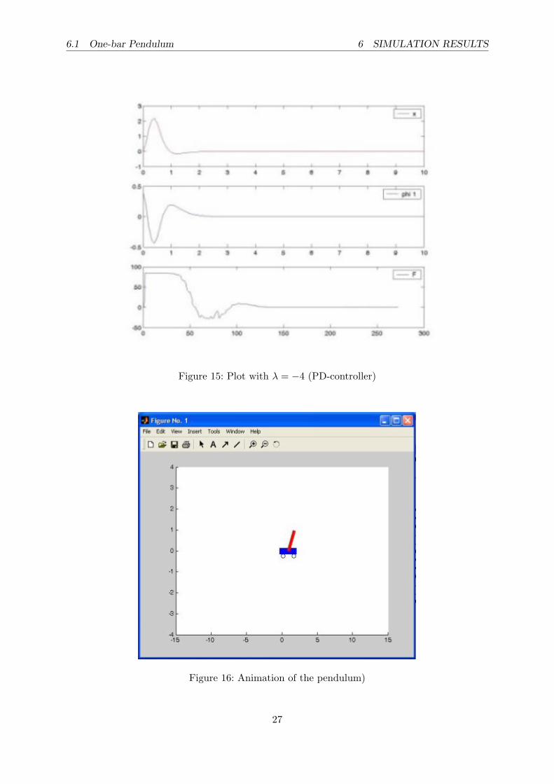
which the pendulum is controlled. In figure 13 to 15 there are plots with an initial deflection of23 degree using λ = −0.5, λ = −1 and λ = −4. The images show, that lower values of λ lead toa faster control of the pendulum. A screenshot of the animation is shown in figure 16.

24

6.1 One-bar Pendulum 6 SIMULATION RESULTS

Figure 12: Plot of x, phi and F with initial deflection greater than 59◦ (PD-controller)

25

6.1 One-bar Pendulum 6 SIMULATION RESULTS

Figure 13: Plot with λ = −0, 5 (PD-controller)

Figure 14: Plot with λ = −1 (PD-controller)

26

6.1 One-bar Pendulum 6 SIMULATION RESULTS

Figure 15: Plot with λ = −4 (PD-controller)

Figure 16: Animation of the pendulum)

27

6.1 One-bar Pendulum 6 SIMULATION RESULTS

6.1.2 Simulation with the neural network

For the simulation of the inverted pendulum we trained a neural network using reinforcementlearning like described in section 6.3. The network had about 4,000 trials to learn. Afterwards itwas able to control a pendulum with an initial angle of about 30 degrees, also depending on theinitial position of the cart. It is not possible to exactly quantify the performance of the neuralnetwork as it is non-deterministic. The reason for the non-determinism is that the decision aboutthe applied force depends also on random values. The applied force is either +10 N or -10 N.This restricts the possible interval of initial angles as for higher deflections, especially in thebeginning of the control cycle, stronger forces are needed.A plot of the cart position, cart velocity, bar angle and bar velocity for an initial angle of 30degrees can be seen in figure 17.

Figure 17: Plot of neural network results with initial angle of 30 ◦

Different trials have shown that starting with random values and training them, a quite similarcontrol behaviour shows up. In figure 18 are examples for the simulation with an initial deflectionof 5.8 degree with two different neural networks each after 1,000 learning steps.After training several neural networks it has shown up that about 4,000 learning steps are enoughso that the neural network can control the inverted pendulum.The following weights have shown good results

a =

−0.72193 −0.38412 −1.7838 −1.0804 −0.44322−0.92651 −0.80744 −1.2158 −0.92695 −0.81483−0.77189 −0.84096 −1.2998 −1.0309 −0.78035−0.83051 −0.53704 −1.4489 −0.91007 −0.55633−0.74199 −0.63616 −1.4718 −0.88074 −0.69155

28

6.1 One-bar Pendulum 6 SIMULATION RESULTS

Figure 18: Plots of neural network results after 1000 learning steps

29

6.2 Double pendulum 7 CONCLUSIONS

b =

−0.46577−0.27866−1.0052−0.610873.0188

c =

−2.4621−0.67372−0.88071−0.84916−1.0529

d =

−0.87518 −1.0326 −0.35068 0.12587 −0.14769−0.76652 −1.0859 −0.21711 0.05435 −0.25859−0.87144 −1.1044 −0.34958 0.021331 −0.37435−0.9112 −1.0643 −0.35439 0.076197 −0.29504−0.88561 −1.1752 −0.22411 −0.011083 −0.33166

e =

0.77669−4.902813.3678.8845−4.4849

f =

−6.223−5.8976−5.623−5.8571−5.6119

We have also tried a feed-forward network with supervised learning, but it has not convergedinto a good local minimum, although we had done many tries. So the stabilisation of the networkwas not possible with this network.

6.2 Double pendulum

We have tried to develop a PD-Controller according to the results of section 5.3.2. We haveapplied many different eigenvalues, also -1 and -3, which were successfully used in [6]. Unfortu-nately the PD-Controller was not able to stabilise the double pendulum. Moreover in the caseof the double pendulum, the control is such complex, that it is not possible to develop a controlstrategy intuitively.Also the approach with the neural network was not successful. With the reinforcement net-work, that showed good results in the one-bar case, is very specialised and cannot be simplytransformed to work for the two-bar case. We could not try the feed-forward network as ourPD-controller did not work well and so we had no teacher for the network.

7 Conclusions

In the paper a model of the n-bar inverted pendulum problem was shown. According to thismodel, the corresponding ODE were listed. Based on this description in state space form, thecontroller equations for the one-bar and the two-bar pendulum were deduced. Moreover, anaproach using neural networks was applied. Two different types of neural networks were used,a feed-forward-network and a reinforcement network.We implemented the model of the inverted n-bar pendulum and the deduced controllers inMatlab. To watch the simulation, we wrote a visualisation of the cart with the pendulum. Wealso added a graphical user interface, for an easy usage of the program.The code was built modular to be extendable, so it is possible to integrate other controllersvery easily. We also put emphasis on the detailed documentation of the code, so that the reuseof the program is enabled.

30

7 CONCLUSIONS

We have not examined the following aspects yet:

• An extension of the inverted pendulum is to allow movements not only in one dimension,but instead to move on a two-dimensional plane. Research concerning this topic is doneby the chair of Professor Schmidhuber by Georg Fette.

• There are many other approaches in the field of machine learning, which could be usedinstead of a feed-forward or a reinforcement network, like genetic algorithms or recurrentnetworks.

• Further controllers can be developped, so that inverted pendulums with more than two barscan be stabilised. But as the equations become much more complex for higher dimensions,it will be more difficult to develop a controller for these cases.

• Another approach is the usage of a fuzzy controller, which was already successfully appliedin this area. The design of a fuzzy controller is also supported of Matlab with the fuzzytoolbox.

31

REFERENCES REFERENCES

References

[1] Anderson, C. W. Code for neuronal networks and reinforcement learning.http://www.cs.colostate.edu/˜anderson/code/ .

[2] Anderson, C. W. Learning to control an inverted pendulum using neural networks. IEEEControl Systems Magazine (1989).

[3] B. Karasozen, P. Rentrop, Y. W. Inverted n-bar model in descriptor and in state spaceform. Mathematical Modelling of Systems, Vol. 4, No. 4, pp. 272 - 285 (1995).

[4] K. Furuta, T. Okutani, H. S. Computer control of a double inverted pendulum. Com-puters and Electrical Engineering, 5, pp. 67 - 84 (1978).

[5] P. J. Larcombe, R. Z. The controllability of a double inverted pendulum by symbolicalgebra analysis. Glasgow University, Proceedings of IEEE - Systems, Man and CyberneticsConference (1993).

[6] Wagner, Y. Modellierung differential-algebraischer gleichungen und neuronale netze zurlosung des stabbalance-problems. TU Munchen, Mathematisches Institut (1994).

32