LINEAR QUADRATIC ESTIMATOR - University of …mocha-java.uccs.edu/ECE5530/ECE5530-CH05.pdf ·...
33
ECE5530: Multivariable Control Systems II. 5–1 LINEAR QUADRATIC ESTIMATOR 5.1: Setting up the optimal state estimator ■ We now start to put the pieces together Least-squares estimation and dynamic systems ➠ Observer. ■ Discrete case first, then convert to continuous case. ■ The filtering aspect will become apparent as we progress. MODEL : Same as before x k C1 D A d x k C w k y k D C d x k C v k : ■ Periodic measurements of system behavior available, but corrupted by noise v k ➠ sensor noise. ■ Process noise w k and sensor noise v k are white. (If not, need to use shaping stuff from before and augment system vector x ). ASSUME : EŒw k Ł D 0I EŒw k w T j Ł D „ w ĩ.k j/ EŒv k Ł D 0I EŒv k v T j Ł D „ v ĩ.k j/ EŒw k v T j Ł D 0 8 k; j EŒx 0 Ł DO x 0: Lecture notes prepared by Dr. Gregory L. Plett. Copyright © 2016, 2010, 2008, 2006, 2004, 2002, 2001, 1999, Gregory L. Plett
-
Upload
nguyentuyen -
Category
Documents
-
view
213 -
download
0
Transcript of LINEAR QUADRATIC ESTIMATOR - University of …mocha-java.uccs.edu/ECE5530/ECE5530-CH05.pdf ·...

ECE5530: Multivariable Control Systems II. 5–1
LINEAR QUADRATIC ESTIMATOR
5.1: Setting up the optimal state estimator
■ We now start to put the pieces together
! Least-squares estimation and dynamic systems ➠ Observer.
■ Discrete case first, then convert to continuous case.
■ The filtering aspect will become apparent as we progress.
MODEL: Same as before
xkC1 D Adxk C wk
yk D Cdxk C vk:
■ Periodic measurements of system behavior available, but corrupted
by noise vk ➠ sensor noise.
■ Process noise wk and sensor noise vk are white. (If not, need to use
shaping stuff from before and augment system vector x).
ASSUME:
EŒwk! D 0I EŒwkwTj ! D „w".k " j /
EŒvk! D 0I EŒvkvTj ! D „v".k " j /
EŒwkvTj ! D 0 8 k; j
EŒx0! D Ox0:
Lecture notes prepared by Dr. Gregory L. Plett. Copyright © 2016, 2010, 2008, 2006, 2004, 2002, 2001, 1999, Gregory L. Plett

ECE5530, LINEAR QUADRATIC ESTIMATOR 5–2
GOAL: Use these periodic measurements of the system output to
develop an optimal estimate of the state xk ! Oxk, and develop a
measure of confidence in this estimate.
TERMINOLOGY:
replacements
k " 1 k k C 1 k C 2
."/."/."/."/ .C/.C/.C/ .C/
■ State estimate is “ Oxk”. Two estimates possible and used:
! One that uses all PRIOR information
# # # yk"2; yk"1 ➠ Ox"k :
! One that uses all POSSIBLE information
# # # yk"2; yk"1; yk
➠ OxCk :
■ Let us analyze one segment
k k C 1
Ox"k OxC
k Ox"kC1 OxC
kC1
STEP I: Measurement update: Use yk to go from Ox"k to OxC
k .
STEP II: Time update: (propagation) Use the (assumed known) plant
model to propagate statistics for OxCk to Ox"
kC1.
■ At each step, we have an estimation error:
QxCk
„ƒ‚…
error
D xk„ƒ‚…
truth
" OxCk
„ƒ‚…
estimate
;
with associated error covariance matrix (assuming/enforcing
EΠQxCk ! D 0).
„Cx;k D E
!
QxCk . QxC
k /T"
D E!
.xk " OxCk /.xk " OxC
k /T"
:
Lecture notes prepared by Dr. Gregory L. Plett. Copyright © 2016, 2010, 2008, 2006, 2004, 2002, 2001, 1999, Gregory L. Plett

ECE5530, LINEAR QUADRATIC ESTIMATOR 5–3
■ Want „Cx;k to be “small”.
STEP I: Assume we have the initial values . Ox"k ; „"
x;k/.
■ Now, use new measurement to find optimal estimates of . OxCk ; „C
x;k/ ➠
Key part of recursive solution.
■ Enforce the constraint that the solution to the update problem
Ox"k ! OxC
k is a linear equation of the form
OxCk D L0
k Ox"k C Lkyk:
■ Updated estimate is a linear combination of previous estimate and
most recent measurement.
■ Lk, L0k time varying matrices; different; yet to be determined.
■ We are looking for the best LINEAR filter.
■ If wk, vk are also Gaussian, it will also turn out this is the BEST filter
possible. No nonlinear filter can do better!
Lecture notes prepared by Dr. Gregory L. Plett. Copyright © 2016, 2010, 2008, 2006, 2004, 2002, 2001, 1999, Gregory L. Plett

ECE5530, LINEAR QUADRATIC ESTIMATOR 5–4
5.2: Deriving the optimal state estimator
STEP I: Solution
■ Assume initial estimate unbiased ➠ EŒ Qx"k ! D 0.
■ Constrain solution so that EŒ QxCk ! D 0 also.
EŒxk " OxCk ! D EŒxk " L0
k Ox"k " Lkyk!
D EŒxk " L0k Ox"
k " Lkyk! C
0‚ …„ ƒ
EŒL0kxk! " EŒL0
kxk!
EŒ QxCk ! D EŒ.I " L0
k " LkCd/xk C L0kxk " L0
k Ox"k
„ ƒ‚ …
L0k Qx"
k
!
D EŒ.I " L0k " LkCd/xk!:
■ To ensure that this estimate is unbiased for all xk, must have
L0k C LkCd D I . Therefore
OxCk D L0
k Ox"k C Lkyk
D .I " LkCd/ Ox"k C Lkyk
D Ox"k C Lk
!
yk " Cd Ox"k
"
„ ƒ‚ …
Innovation
where the innovation is the error in our estimate, or “what is new” in
this measurement.
■ Exactly the same form as we have seen before in the updates we
have looked at! Need a good way to choose “blending factor” Lk.
Estimate covariance
■ Since the estimation error has zero mean, the covariance matrix is
„x;k D EŒ Qxk QxTk !.
Lecture notes prepared by Dr. Gregory L. Plett. Copyright © 2016, 2010, 2008, 2006, 2004, 2002, 2001, 1999, Gregory L. Plett

ECE5530, LINEAR QUADRATIC ESTIMATOR 5–5
■ Need to look at „"x;k and „C
x;k to see how covariance is changed by a
measurement.
■ Then, pick Lk for “optimal blending”.
Optimization
■ We will choose Lk to minimize the sum of the squares of the
estimation error vector:
Jk D EŒ#
QxCk
$T QxC
k !:
■ Equivalent to minimizing the “length” squared of the error vector,
which seems like an appealing objective.
■ Note that we can rewrite the cost in terms of the error covariance
matrix
Jk D traceŒ„Cx;k!
(recall xT x D traceŒxxT !).
Covariance update
■ First, we must write „Cx;k in terms of „"
x;k and the measurement noise.
■ Know OxCk D .I " LkCd/ Ox"
k C Lkyk. Therefore, estimation error
dynamics given by
QxCk D xk " OxC
k
D xk " .I " LkCd/ Ox"k " Lk.Cdxk C vk/
D .I " LkCd/ Qx"k " Lkvk:
Lecture notes prepared by Dr. Gregory L. Plett. Copyright © 2016, 2010, 2008, 2006, 2004, 2002, 2001, 1999, Gregory L. Plett

ECE5530, LINEAR QUADRATIC ESTIMATOR 5–6
■ Now, form
„Cx;k D EŒ QxC
k
#
QxCk
$T !
D EŒf.I " LkCd/ Qx"k " Lkvkgf.I " LkCd/ Qx"
k " LkvkgT !:
■ As before, three terms,
1. EŒ.I " LkCd/ Qx"k
#
Qx"k
$T .I " LkCd/T ! D .I " LkCd/„"
x;k.I " LkCd/T .
2. EŒLkvkvTk LT
k ! D Lk„vLTk .
3. EΠQx"k vT
k ! D 0 since prior estimate error is uncorrelated with the
measurement noise at this time step.
■ Therefore, for any Lk,
„Cx;k D .I " LkCd/„"
x;k.I " LkCd/T C Lk„vLTk :
■ These two equations tell us how to update Qxk and „x;k, given any Lk.
■ Now, optimize to find best Lk.
■ The “trace” operator makes life quite easy since we have
d trace.AB/
dAD BT ; AB square
d trace.ACAT /
dAD 2AC; C symmetric:
■ FormdJk
dLkD 0 for optimal gain. Recall
Jk D EΠQxTk
C QxCk ! D trace.„C
x;k/
D trace#
.I " LkCd/„"x;k.I " LkCd/T
$
C trace.Lk„vLTk /
■ Then,dJk
dLk
D "2„"x;kC T
d C 2Lk.Cd„"x;kC T
d C „v/ D 0
Lecture notes prepared by Dr. Gregory L. Plett. Copyright © 2016, 2010, 2008, 2006, 2004, 2002, 2001, 1999, Gregory L. Plett

ECE5530, LINEAR QUADRATIC ESTIMATOR 5–7
which gives
L$k D „"
x;kC Td
!
Cd„"x;kC T
d C „v
""1
which is the Kalman gain matrix—minimizing gain.
■ Can show that with this gain
„Cx;k D .I " L$
kCd/„"x;k
D
%
The optimized value of the updated
error covariance matrix.
&
■ Thus, in terms of the mean-square estimation error,
Lk D „"x;kC T
d
!
Cd„"x;kC T
d C „v
""1
is the optimal blending ratio ➠ Very similar form to the gain matrices
studied earlier.
(End of STEP I, measurement update).
STEP II: Time update (propagation).
■ Have developed update estimates at time “kC”.
■ Need to propagate to develop predictions of the best estimate at time
“.k C 1/"”.
■ Have already studied this case. Using known model and process
noise covariance,
Ox"kC1 D Ad OxC
k .C deterministic input/
„"x;kC1 D Ad„C
x;kATd C „w:
Lecture notes prepared by Dr. Gregory L. Plett. Copyright © 2016, 2010, 2008, 2006, 2004, 2002, 2001, 1999, Gregory L. Plett

ECE5530, LINEAR QUADRATIC ESTIMATOR 5–8
5.3: Kalman filter loop
■ We can combine the parts that make up this one segment
.#/"k ) .#/"
kC1 to form a recursion:
Prior estimates Ox"k ; „"
x;kUsually initialize with Ox0; „x;0
Compute Kalman gain
Lk D „"x;kC T
d
!
Cd „"x;kC T
d C „v
""1
Update estimate with yk
OxCk D Ox"
k C Lk
!
yk " Cd Ox"k
"
Update covariance„C
x;k D .I " LkCd /„"x;k
PropagateOx"kC1 D Ad OxC
k
„"x;kC1 D Ad „C
x;kATd C „w
ykk ! k C 1
■ “Simple” to perform on a digital computer.
EXAMPLE: Px.t/ D w.t/, "t D 1, Sw D 1.
■ Independent noisy measurements y.t/ D x.t/ C v.t/.
■ Standard deviation of measurement noise #v D 1=2.
■ Convert continuous to discrete
xk D Adxk"1 C wk"1; EŒwkwl ! D „w".k " l/:
! Find Ad from zero-order-hold equivalent: Ad D 1.
! Find „w using „w D
Z 1
0
e0Swe0 dt D 1.
! Measurement equation, yk D Cdxk C vk.
EŒvkvk! D „v D #2v D 1=4; Cd D 1:
! Assume that there is no initial uncertainty. Ox"0 D 0 and „"
x;0 D 0.
Lecture notes prepared by Dr. Gregory L. Plett. Copyright © 2016, 2010, 2008, 2006, 2004, 2002, 2001, 1999, Gregory L. Plett

ECE5530, LINEAR QUADRATIC ESTIMATOR 5–9
Time step 0:
■ L0 D „"x;0C
Td .Cd„"
x;0CTd C „v/"1 D 0.
■ OxC0 D Ox"
0 C L0.y0 " Cd Ox"0 / D Ox"
0 D 0.
■ „Cx;0 D .I " L0Cd/„"
x;0 D „"x;0 D 0.
■ Ox"1 D Ad OxC
0 D 0 and „"x;1 D Ad„C
x;0ATd C „w D 0 C 1 D 1.
Time step 1:
■ L1 D „"x;1C
Td .Cd„"
x;1CTd C „v/"1 D 1 # 1.1 # 1 # 1 C 1=4/"1 D 4=5.
■ OxC1 D Ox"
1 C L1.y1 " Cd Ox"1 / D 0 C .4=5/y1 D .4=5/y1.
■ „Cx;1 D .I " L1Cd/„"
x;1 D 1=5.
■ Ox"2 D Ad OxC
1 D .4=5/y1 and „"x;2 D Ad„C
x;1ATd C „w D .1=5/ C 1 D 6=5.
Time step 2:
■ L2 D „"x;2C
Td .Cd„"
x;2CTd C „v/"1 D .6=5/.6=5 C 1=4/"1 D 24=29.
■ OxC2 D Ox"
2 C L2.y2 " Cd Ox"2 / D .4=29/y1 C .24=29/y2.
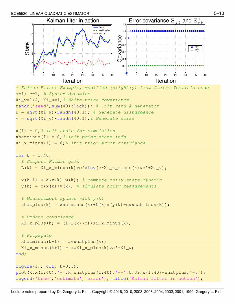
■ „Cx;2 D 6=29 and so forth, hopefully to steady state.
„"x;0 D 0 „"
x;1 D 1 „"x;2 D 1:2 „"
x;3 D 1:207
# % # % # % # %
„Cx;0 D 0 „C
x;1 D 0:2 „Cx;2 D 0:207 „C
x;3 D 0:2071
■ Covariance increases during propagation and is then reduced by
each measurement.
■ Covariance still oscillates at steady state between „"x;ss and „C
x;ss.
Lecture notes prepared by Dr. Gregory L. Plett. Copyright © 2016, 2010, 2008, 2006, 2004, 2002, 2001, 1999, Gregory L. Plett
ECE5530, LINEAR QUADRATIC ESTIMATOR 5–10
0 5 10 15 20 25 30 35 40−2
0
2
4
6
8true estimateerror
Iteration
Sta
teKalman filter in action
0 5 10 15 20 25 30 35 400
0.2
0.4
0.6
0.8
1
1.2
1.4
Iteration
Cova
riance
Error covariance „"x;k and „C
x;k
„!x
„Cx
% Kalman Filter Example, modified (slightly) from Claire Tomlin's code
a=1; c=1; % System dynamics
Xi_v=1/4; Xi_w=1;% White noise covariance
randn('seed',sum(40*clock)); % Init rand # generator
w = sqrt(Xi_w)*randn(40,1); % Generate disturbance
v = sqrt(Xi_v)*randn(40,1);% Generate noise
x(1) = 0;% init state for simulation
xhatminus(1) = 0;% init prior state info
Xi_x_minus(1) = 0;% init prior error covariance
for k = 1:40,
% Compute Kalman gain
L(k) = Xi_x_minus(k)*c'*inv(c*Xi_x_minus(k)*c'+Xi_v);
x(k+1) = a*x(k)+w(k); % compute noisy state dynamic
y(k) = c*x(k)+v(k); % simulate noisy measurements
% Measurement update with y(k)
xhatplus(k) = xhatminus(k)+L(k)*(y(k)-c*xhatminus(k));
% Update covariance
Xi_x_plus(k) = (1-L(k)*c)*Xi_x_minus(k);
% Propagate
xhatminus(k+1) = a*xhatplus(k);
Xi_x_minus(k+1) = a*Xi_x_plus(k)*a'+Xi_w;
end;
figure(1); clf; k=0:39;
plot(k,x(1:40),'-',k,xhatplus(1:40),'--',0:39,x(1:40)-xhatplus,'-.');
legend('true','estimate','error'); title('Kalman filter in action');
Lecture notes prepared by Dr. Gregory L. Plett. Copyright © 2016, 2010, 2008, 2006, 2004, 2002, 2001, 1999, Gregory L. Plett

ECE5530, LINEAR QUADRATIC ESTIMATOR 5–11
xlabel('Iteration'); ylabel('State'); grid;
figure(2); clf;
plot(k,Xi_x_minus(1:40),'o',k,Xi_x_plus(1:40),'+');
grid; legend('Xi_x^{-}','Xi_x^{+}',0);
title('Error covariance before (o) and after ^{+} meas. update');
xlabel('Iteration'); ylabel('Covariance');
Discrete Kalman filter versus RLS
KALMAN: First the covariance matrix:
„Cx;k D .I " LkCd/„"
x;k
D „"x;k " „"
x;kC Td
!
Cd„"x;kC T
d C „v
""1Cd„"
x;k:
■ Now, use matrix inversion lemma (proof in book appendix)!
NA"1 C NBT NC "1 NB""1
D NA " NA NBT!
NB NA NBT C NC""1 NB NA
where we substitute
NA D „"x;k
NB D CdNC D „v:
■ Thenh
„Cx;k
i
"1 D!
„"x;k
""1 C C T
d „"1v Cd :
■ For the gain, use the following form of the matrix inversion lemma:!
NA"1 C NBT NC "1 NB""1 NBT NC "1 D NA NBT
!NB NA NBT C NC
""1
with the same substitutions (proof in notes appendix).
■ So:
Lk D „"x;kC T
d
!
Cd„"x;kC T
d C „v
""1
D!#
„"x;k
$"1 C C T
d „"1v Cd
""1C T
d „"1v
D „Cx;kC T
d „"1v :
Lecture notes prepared by Dr. Gregory L. Plett. Copyright © 2016, 2010, 2008, 2006, 2004, 2002, 2001, 1999, Gregory L. Plett

ECE5530, LINEAR QUADRATIC ESTIMATOR 5–12
RLS: Covariance update was
Q"1kC1 D Q"1
k C H TkC1R
"1kC1HkC1:
■ The gain was
gain D QkC1HTkC1R
"1kC1:
■ Therefore, measurement update step of Kalman filter is the same as
the recursive form of the maximum-likelihood estimate (when v in
y D Hx C v is Gaussian, OxML is linear).
! Therefore, if wk is Gaussian, a linear filter is the best filter possible!
No nonlinear filter can do better!
■ Time update is additional step necessary when estimating a moving
(dynamic) state vector.
Lecture notes prepared by Dr. Gregory L. Plett. Copyright © 2016, 2010, 2008, 2006, 2004, 2002, 2001, 1999, Gregory L. Plett

ECE5530, LINEAR QUADRATIC ESTIMATOR 5–13
5.4: Continuous-time filters
GOAL: Develop an estimator Ox.t/ that is a linear function of
measurements y.$/, 0 % $ % t , and minimizes the function
E!
.x.t/ " Ox.t//T .x.t/ " Ox.t//"
:
ASSUMED: Dynamics of linear system are
Px.t/ D Ax.t/ C Bww.t/
y.t/ D Cyx.t/ C v.t/
and EŒw.t/! D EŒv.t/! D 0; EŒw.t1/w.t2/T ! D Swı.t1 " t2/,
EŒv.t1/v.t2/T ! D Svı.t1 " t2/, EŒw.t1/v.t2/! D 0, Sw > 0, Sv > 0, Ox.0/ and
„x.0/ given.
APPROACH: As before, analyze discrete case as "t ! 0.
■ To proceed, we must relate the discrete and continuous sensor
noises. (We already saw how to relate process noises).
■ One approach: Use discrete noise ("t small)
vk D1
"t
Z "t
0
v.t/ dt .average value/:
■ Then,
„v D EŒvkvTk ! D
1
"t 2
Z "t
0
Z "t
0
EŒv.%/v.$/T ! d% d$
D1
"t 2# "t # Sv D
Sv
"t:
■ As "t ! 0, the discrete noise tends to infinite pulse covariance with
weight Sv, similar to Svı.t/.
Lecture notes prepared by Dr. Gregory L. Plett. Copyright © 2016, 2010, 2008, 2006, 2004, 2002, 2001, 1999, Gregory L. Plett

ECE5530, LINEAR QUADRATIC ESTIMATOR 5–14
Conversion
■ Recall
! „"x;kC1 D Ad„C
x;kATd C „w.
! „Cx;k D .I " LkCd/„"
x;k.
■ With malice aforethought, consider
Lk
"tD
„"x;kC T
d
"t
!
Cd„"x;kC T
d C „v
""1
D „"x;kC T
d
!
Cd„"x;kC T
d "t C „v"t""1
:
■ As "t ! 0, if „"x;k finite,
Cd„"x;kC T
d "t ! 0
„v"t ! Sv
„"x;k ! „x.t/
Cd ! Cy
9
>>>>=
>>>>;
as "t ! 0Lk
"t! L.t/ D „x.t/C T
y S"1v :
■ Already looked at propagation case
„"x;kC1 D Ad„C
x;kATd C „w
& .I C A"t/„Cx;k.I C A"t/T C BwSwBT
w "t
D „Cx;k C "t
h
A„Cx;k C „C
x;kAT C BwSwBTw
i
C o."t 2/;
but „Cx;k D „"
x;k " LkCd„"x;k . . . combine. . .
„"x;kC1 D „"
x;k " LkCd„"x;k
C"th
A„"x;k " ALkCd„"
x;k C „"x;kAT
"LkCd„"x;kAT C BwSwBT
w
i
Co."t 2/:
Lecture notes prepared by Dr. Gregory L. Plett. Copyright © 2016, 2010, 2008, 2006, 2004, 2002, 2001, 1999, Gregory L. Plett

ECE5530, LINEAR QUADRATIC ESTIMATOR 5–15
■ Rearrange. . .
„"x;kC1 " „"
x;k
"tD
"Lk
"tCd„"
x;k C A„"x;k C „"
x;kAT C BwSwBTw
"ALkCd„"x;k " LkCd„"
x;kAT C o."t /:
■ As "t ! 0, LHS ! P„x.t/, Cd ! Cy,Lk
"t! L.t/, „"
x;k ! „x.t/ and
ALkCd„"x;k ! 0.
Resulting expression
P„x.t/ D
Riccati for measurement update‚ …„ ƒ
A„x.t/ C „x.t/AT C BwSwBTw
„ ƒ‚ …
Lyapunov for propagation
" „x.t/C Ty S"1
v Cy„x.t/„ ƒ‚ …
'0
:
■ Matrix RICCATI equation for error covariance.
■ Equation includes the following impact on P„x.t/:
! A„x.t/ C „x.t/AT➠ Homogeneous part.
! BwSwBTw ➠ Increase due to process noise.
! „x.t/C Ty S"1
v Cy„x.t/ ➠ Decrease due to measurements.
Culture
Count Jacopo Francesco Riccati (1676–1754) was an Italian savant who wrote on mathematics,
physics, and philosophy. He was chiefly responsible for introducing the ideas of Newton to Italy.
At one point he was offered the presidency of the St. Petersburg Academy of Sciences but
understandably he preferred the leisure and comfort of his aristocratic life in Italy to
administrative responsibilities in Russia. Though widely known in scientific circles of his time,
he now survives only through the differential equation bearing his name. Even this was an
accident of history, for Riccati merely discussed special cases of this equation without offering
any solutions, and most of these special cases were successfully treated by various members
of the Bernoulli family. The details of this complex story can be found in G. N. Watson “A
treatise on the Theory of Bessel Functions.” 2d ed., pp. 1–3, Cambridge, London, 1944. The
special Riccati equation Py C by2 D cxm is known to be solvable in finite terms if and only if the
exponent m is "2 or of the form "4k=.2k C 1/ for some integer k.
Lecture notes prepared by Dr. Gregory L. Plett. Copyright © 2016, 2010, 2008, 2006, 2004, 2002, 2001, 1999, Gregory L. Plett

ECE5530, LINEAR QUADRATIC ESTIMATOR 5–16
(Taken from “Differential Equations with Applications and Historical Notes” by George F.
Simmons).
State-Estimate Update
■ Recall
1. Ox"k D Ad OxC
k"1.
2. OxCk D Ox"
k C Lk.yk " Cd Ox"k /.
■ Substitute (1) into (2)
OxCk D Ad OxC
k"1 C Lk.yk " CdAd OxCk"1/:
■ Substitute:
OxCk D .I C A"t/ OxC
k"1 C Lk
'
yk " Cd.I C A"t/ Oxk"1
(
:
■ So,
OxCk " OxC
k"1
"tD A OxC
k"1 CLk
"t
'
yk " Cd OxCk"1 " CdA"t OxC
k"1
(
:
■ Then,
POx.t/ D A Ox.t/ C L.t/!
y.t/ " Cy Ox.t/"
L.t/ D „x.t/C Ty S"1
v
P„x.t/ D A„x.t/ C „x.t/AT C BwSwBTw " „x.t/C T
y S"1v Cy„x.t/:
■ This is called a “Kalman–Bucy” filter, or a continuous-time Kalman
filter/estimator.
EXAMPLE: Estimate the value of a constant given continuous
measurements of x corrupted by Gaussian white noise.
Px D 0 .trivial dynamics of constant/
Lecture notes prepared by Dr. Gregory L. Plett. Copyright © 2016, 2010, 2008, 2006, 2004, 2002, 2001, 1999, Gregory L. Plett

ECE5530, LINEAR QUADRATIC ESTIMATOR 5–17
y D x C v;
where v ( N .0; Sv/. Then A D Bw D Sw D 0.
■ The Riccati equation becomes: P„x.t/ D "„2x.t/=Sv.
■ Integrate:Z „x.t/
„x;0
d„x.$/
„2x.$/
D "1
Sv
Z t
0
d$
"„"1x .$/
ˇˇ„x.t/
„x;0D "t=Sv
1
„x;0"
1
„x.t/D "t=Sv
1
„x;0C
t
SvD
1
„x.t/
„x.t/ D„x;0Sv
Sv C „x;0tI
L.t/ D „x.t/=Sv D„x;0
Sv C „x;0t:
■ As t ! 1, L.t/ ! 0, so that Ox.t/ ! constant.
POx.t/ D„x;0
Sv C „x;0t„ ƒ‚ …
L.t/
Œy.t/ " Ox.t/! ! 0:
Lecture notes prepared by Dr. Gregory L. Plett. Copyright © 2016, 2010, 2008, 2006, 2004, 2002, 2001, 1999, Gregory L. Plett

ECE5530, LINEAR QUADRATIC ESTIMATOR 5–18
5.5: Steady-state Kalman filters
■ Several examples have begun to demonstrate that the filter gains can
have a transient and then settle to constant values.
Steady stateL.t/
■ Since the estimator will typically be running for a long time, most of
the operations will occur with the filter in the steady-state region.
■ Therefore, recursive/differential equations do not need to be solved!
Steady-state solution
■ The Kalman gain depends on state covariance, which for a discrete-
time system has two steady-state solutions: „"x;ss and „C
x;ss. Then,
Lss D „Cx;ssC
Td „"1
v :
■ Consider the filter loop as k ! 1
„"x;ss D Ad„C
x;ssATd C „w
„Cx;ss D „"
x;ss " „"x;ssC
Td
!
Cd„"x;ssC
Td C „v
""1Cd„"
x;ss:
■ Combine these two to get
„"x;ss D „w C Ad„"
x;ssATd "
Ad„"x;ssC
Td
!
Cd„"x;ssC
Td C „v
""1Cd„"
x;ssATd :
■ One matrix equation, one
matrix unknown ➠ dlqe.m
k k C 1 k C 2 k C 3
„x
Lecture notes prepared by Dr. Gregory L. Plett. Copyright © 2016, 2010, 2008, 2006, 2004, 2002, 2001, 1999, Gregory L. Plett

ECE5530, LINEAR QUADRATIC ESTIMATOR 5–19
EXAMPLE: xkC1 D xk C wk. yk D xk C vk. Steady-state covariance?
■ Let EŒwk! D EŒvk! D 0, EŒwkwl ! D 1".k " l/, EŒvkvl ! D 2".k " l/
■ EŒx0! D Ox0 and EŒ.x0 " Ox0/.x0 " Ox0/! D „x;0.
■ Notice Ad D 1, Cd D 1, „w D 1 and „v D 2.'
„Cx;k
(
"1 D#
„"x;k
$"1 C C T
d „"1v Cd
„Cx;k D
11
„"x;k
C 12
D2„"
x;k
2 C „"x;k
:
„"x;kC1 D Ad„C
x;kATd C „w D „C
x;k C 1 D2„"
x;k
2 C „"x;k
C 1
„"x;ss D
2„"x;ss
2 C „"x;ss
C 1
which gives us „"x;ss D 2 and „C
x;ss D 1.
„"x;0 D 1 „"
x;1 D 3 „"x;2 D 11=5 „"
x;3 D 43=21
# % # % # % # %
„Cx;0 D 2 „C
x;1 D 6=5 „Cx;2 D 22=21 „C
x;3 D 86=85
Steady-state in continuous time
■ The same kind of result often holds for LTI continuous-time systems.
■ The steady-state Kalman gain is associated with P„x.t/ ! 0, giving
the algebraic Riccati equation (ARE)
A„x C „xAT C BwSwBTw " „xC T
y S"1v Cy„x D 0
and
L D „xC Ty S"1
v :
Lecture notes prepared by Dr. Gregory L. Plett. Copyright © 2016, 2010, 2008, 2006, 2004, 2002, 2001, 1999, Gregory L. Plett

ECE5530, LINEAR QUADRATIC ESTIMATOR 5–20
■ Same as time-varying case, but with constant „x and L. care.m
■ Tradeoff between sensor and process noise now explicit:
L D „xC Ty S"1
v .
! If uncertain about estimate („x large), then innovation .y " Cy Ox/
weighted heavily (big L).
! If Sv small (measurements accurate) then new measurements
highly weighted (big L).
■ We can think of „xC Ty S"1
v as analogous to SNR.
NOTE: Continuous case requires Sv > 0 (S"1v explicit) but discrete does
not („"1v can be avoided).
Stability of steady-state Kalman filter
■ Steady-state gain is much easier to compute/use than time-varying
solution.
■ Small performance reduction if we use steady-state value for ALL
time since transient region is quite short (relatively). But, what can we
say about stability?
CTS SYSTEM:
Px.t/ D Ax.t/ C Bww.t/
y.t/ D Cyx.t/ C v.t/
where w ( N .0; Sw/ and v ( N .0; Sv/; w; v white and independent.
ASSUME:
1. Sv > 0, Sw > 0.
Lecture notes prepared by Dr. Gregory L. Plett. Copyright © 2016, 2010, 2008, 2006, 2004, 2002, 2001, 1999, Gregory L. Plett

ECE5530, LINEAR QUADRATIC ESTIMATOR 5–21
2. All plant dynamics constant
3. ŒA; Cy! detectable (unstable modes observable)
4. ŒA; Bw! stabilizable (unstable modes controllable)
■ Time-varying Kalman gains for this time-invariant system satisfy
P„x D A„x C „xAT C BwSwBTw " „xC T
y S"1v Cy„x
L D „xC Ty S"1
v ;
„x;0 given.
■ With the above assumptions, „x.t/ ! „x;ss regardless of „x;0 as
t ! 1, where „x;ss solves
0 D A„x;ss C „x;ssAT C BwSwBT
w " „x;ssCTy S"1
v Cy„x;ss:
■ Stabilizable/detectable implies „x;ss ' 0 (unique)
■ „x;ss > 0 iff ŒA; Bw! controllable.
■ If „x;ss exists, the steady-state optimal estimator
POx D A Ox C Lss.y.t/ " Cy Ox.t//
Lss D „x;ssCTy S"1
v
is asymptotically stable if (1)–(4) hold.
Big conclusion
1. Time-varying Kalman filter gains provide PERFORMANCE OPTIMAL
filter design, but,
2. Under MILD conditions, we can show that the closed-loop estimation
error dynamics are stable when we use the steady-state gains for all
time ➠ BIG computational savings.
Lecture notes prepared by Dr. Gregory L. Plett. Copyright © 2016, 2010, 2008, 2006, 2004, 2002, 2001, 1999, Gregory L. Plett

ECE5530, LINEAR QUADRATIC ESTIMATOR 5–22
5.6: Frequency-domain interpretation
■ We are interested in finding the estimation-error dynamics. We start
with the plant dynamics:
Px D Ax C Buu C Bww
y D Cyx C v
where w ( N .0; Sw/, BwSwBTw > 0, v ( N .0; Sv/, Sv > 0; w; v white
and independent, ŒA; Cy! observable.
■ Strong form of assumptions.
■ Steady-state Kalman filter:
POx D A Ox C Buu C L.y " Cy Ox/:
■ This gives estimation error dynamics: Qx D x " Ox
PQx D Px " POx D Ax C Bww "!
.A " LCy/ Ox C L.Cyx C v/"
D .A " LCy/ Qx C Bww " Lv:
■ Filter stability governed by eigenvalues of .A " LCy/.
■ Equation makes explicit the tradeoff between:
! Speed of estimator error decay (L big, eig.A " LCy/ far in LHP)
! Susceptibility of estimator error to being corrupted by sensor
noise. (L small so Lv small).
■ Kalman filter selects the optimal balance between these two goals.
■ Have POx D A Ox C L.y " Cy Ox/ . . . (steady-state filter)
Lecture notes prepared by Dr. Gregory L. Plett. Copyright © 2016, 2010, 2008, 2006, 2004, 2002, 2001, 1999, Gregory L. Plett

ECE5530, LINEAR QUADRATIC ESTIMATOR 5–23
■ Laplace transform both sides. . . (assume scalar state for now)
OX.s/
Y.s/D
L
s " A C LCyD
LLCy"A
sLCy"A
C 1:
■ Pole at s D ".LCy " A/ and dc-gain of L=.LCy " A/.
■ This is the transfer function of the filter applied to the measurements
to form the estimate Ox (low-pass).
■ Increasing L pushes the filter transfer function up and out.
Increasing L
f
ˇˇˇ OX=Y
ˇˇˇ
■ Eventually, estimate would be too corrupted by the noise in the
measurements.
■ Note that balancing the sensor-noise impact done with respect to the
process noise .Bww/.
■ It turns out that the ratio Sw=Sv plays a key role in the selection of L.
EXAMPLE: System driven by noise
Px D w
y D x C v
where EŒw! D EŒv! D 0 and w and v independent;
EŒw.t/w.t C $/! D Swı.$/ and EŒv.t/v.t C $/! D Svı.$/.
■ EŒx.0/! D 0, EŒx.0/2! D „x.0/.
Lecture notes prepared by Dr. Gregory L. Plett. Copyright © 2016, 2010, 2008, 2006, 2004, 2002, 2001, 1999, Gregory L. Plett

ECE5530, LINEAR QUADRATIC ESTIMATOR 5–24
■ The optimal filter is
POx D„x.t/
Sv
.y " Ox/
„x.t/ Dp
SwSv1 C be"2˛t
1 " be"2˛t;
where ˛ Dp
Sw=Sv and b D .„x.0/ "p
SwSv/=.„x.0/ Cp
SwSv/.
■ Convergence speed of „x.t/ determined by Sw=Sv.
■ Steady-state:
„x.t/ ! „x;ss Dp
SwSv
Lss D„x;ss
SvD
p
Sw=Sv:
Therefore, steady-state filter:
POx D "
s
Sw
SvOx C
s
Sw
Svy;
and the closed-loop pole location determined by Sw=Sv.
■ If Sw=Sv small, sensors are relatively noisy.
■ If Sw=Sv large, sensors relatively clean.
More “culture”
■ There are three main types of Kalman filter:
1. We have concentrated on the “filtering problem”.
■ Use data up to and
including the current time
to provide an estimate for
the current time.
DATA
Current time
Ox.t/
Lecture notes prepared by Dr. Gregory L. Plett. Copyright © 2016, 2010, 2008, 2006, 2004, 2002, 2001, 1999, Gregory L. Plett

ECE5530, LINEAR QUADRATIC ESTIMATOR 5–25
2. The “smoothing problem” (offline, post-analysis)
■ Use data up to and
including the current time
to provide an estimate for
a past time.
DATA
Current timePrior time
Ox.to/
3. The “prediction problem”
■ Use data up to and
including the current time
to provide an estimate for
a future time.
DATA
Current time Futuretime
Ox.tf /
■ All three filters have application to control theory, but #2 and #3 are
used more often by signal-processing people.
Lecture notes prepared by Dr. Gregory L. Plett. Copyright © 2016, 2010, 2008, 2006, 2004, 2002, 2001, 1999, Gregory L. Plett
ECE5530, LINEAR QUADRATIC ESTIMATOR 5–26
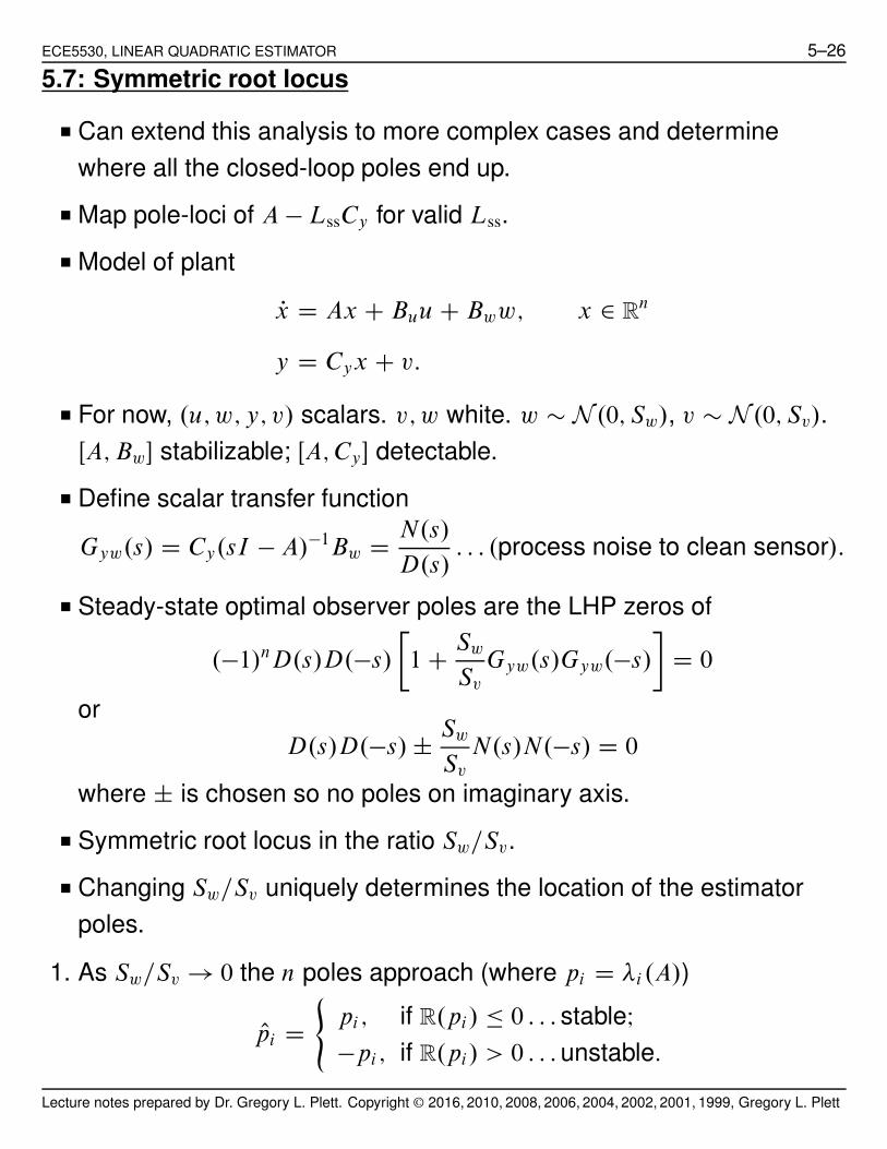
5.7: Symmetric root locus
■ Can extend this analysis to more complex cases and determine
where all the closed-loop poles end up.
■ Map pole-loci of A " LssCy for valid Lss.
■ Model of plant
Px D Ax C Buu C Bww; x 2 Rn
y D Cyx C v:
■ For now, .u; w; y; v/ scalars. v; w white. w ( N .0; Sw/, v ( N .0; Sv/.
ŒA; Bw! stabilizable; ŒA; Cy! detectable.
■ Define scalar transfer function
Gyw.s/ D Cy.sI " A/"1Bw DN.s/
D.s/: : : .process noise to clean sensor/:
■ Steady-state optimal observer poles are the LHP zeros of
."1/nD.s/D."s/
%
1 CSw
Sv
Gyw.s/Gyw."s/
&
D 0
or
D.s/D."s/ ˙Sw
Sv
N.s/N."s/ D 0
where ˙ is chosen so no poles on imaginary axis.
■ Symmetric root locus in the ratio Sw=Sv.
■ Changing Sw=Sv uniquely determines the location of the estimator
poles.
1. As Sw=Sv ! 0 the n poles approach (where pi D &i .A/)
Opi D
(
pi; if R.pi/ % 0 : : : stableI
"pi; if R.pi/ > 0 : : : unstable:
Lecture notes prepared by Dr. Gregory L. Plett. Copyright © 2016, 2010, 2008, 2006, 2004, 2002, 2001, 1999, Gregory L. Plett

ECE5530, LINEAR QUADRATIC ESTIMATOR 5–27
■ As sensors become relatively noisy, filter gains very low.
Essentially open-loop, but must be stable.
2. As Sw=Sv ! 1, —low sensor noise, high bandwidth—assume N.s/
has m roots ´i
(a) m of the n poles approach
Opi D
(
´i ; if R.´i/ % 0I
"´i ; if R.´i/ > 0;
the finite zeros of N.s/=D.s/.
(b) Remaining n " m poles asymptotically approach straight lines that
intersect at origin with angles
˙l'
n " ml D 0; 1; : : : .n " m " 1/=2 n " m odd
˙.l C 1=2/'
n " ml D 0; 1; : : : .n " m/=2 " 1 n " m even;
a BUTTERWORTH configuration.
Butterworth examples
n " m D 1 n " m D 2 n " m D 3
R.s/ R.s/R.s/
I.s/ I.s/I.s/
45ı 72ı
■ Remember, these are only asymptotic trajectories for the poles. We
can use standard root-locus arguments to find out where the rest of
the poles end up at intermediate values of Sw=Sv.
■ Note the key role played by the ratio Sw=Sv.
Lecture notes prepared by Dr. Gregory L. Plett. Copyright © 2016, 2010, 2008, 2006, 2004, 2002, 2001, 1999, Gregory L. Plett

ECE5530, LINEAR QUADRATIC ESTIMATOR 5–28
EXAMPLE: Undamped harmonic oscillator."
Px1
Px2
#
D
"
0 1
"!2o 0
# "
x1
x2
#
C
"
0
1
#
w
and w ( N .0; 1/, v ( N .0; Sv/.
y D x2 C v:
■ Location of optimal poles?
Gyw.s/ Dh
0 1i
( "
s 0
0 s
#
"
"
0 1
"!2o 0
#) "1 "
0
1
#
Ds
s2 C !2o
DN.s/
D.s/:
■ Need to find stable solutions of
.s2 C !2o/2 "
1
Sv.s2/ D 0
or
1 "1
Sv
s2
.s2 C !2o/2
D 0:
Sv ! 1
Sv ! 0 Sv ! 0
■ As Sv ! 0 (low sensor noise), one observer pole tends to the origin
(shielded from process noise by system zero at origin). The other
pole ! "1, which essentially results in differentiation of the output to
determine the state.
■ As Sv ! 1 (high sensor noise), poles revert to the open-loop poles
(open-loop observer).
Lecture notes prepared by Dr. Gregory L. Plett. Copyright © 2016, 2010, 2008, 2006, 2004, 2002, 2001, 1999, Gregory L. Plett

ECE5530, LINEAR QUADRATIC ESTIMATOR 5–29
5.8: Relationship between LQE and LQR
■ For LQR, we solve the Riccati equation
" PP .t/ D P.t/A C AT P.t/ C Q " P.t/BuR"1BTu P.t/:
P.t/ is the linear function relating the costate to the state
(&.t/ D P.t/x.t/), Q is the state-weighting penalty and R is the
control-weighting penalty.
■ For LQE, we found that we need to solve the Riccati equation
P„x.t/ D „x.t/AT C A„x.t/ C BwSwBTw " „x.t/C T
y S"1v Cy„x.t/:
„x.t/ is the error covariance matrix, Sw is the process noise spectral
density and Sv is the measurement noise spectral density.
■ The LQR and LQE Riccati equations are duals. First note that LQR is
solved backward in time. If it were to be solved forward in time we
would have
PP .t/ D P.t/A C AT P.t/ C Q " P.t/BuR"1BTu P.t/:
■ Then, replace A , AT , Bu , C Ty , K , L, Q , BwSwBT
w , R , Sv
and P , „x to notice the duality.
■ Duality is explored in further detail in the text to show that LQE is H2
optimal estimation when cast in a certain framework just as LQR is
H2 optimal control in a similar specific framework.
Solving for the gain matrix L.t/
■ Here, we use duality to formulate an estimator Hamiltonian matrix,
which may be used to solve the estimator Riccati equation.
Lecture notes prepared by Dr. Gregory L. Plett. Copyright © 2016, 2010, 2008, 2006, 2004, 2002, 2001, 1999, Gregory L. Plett
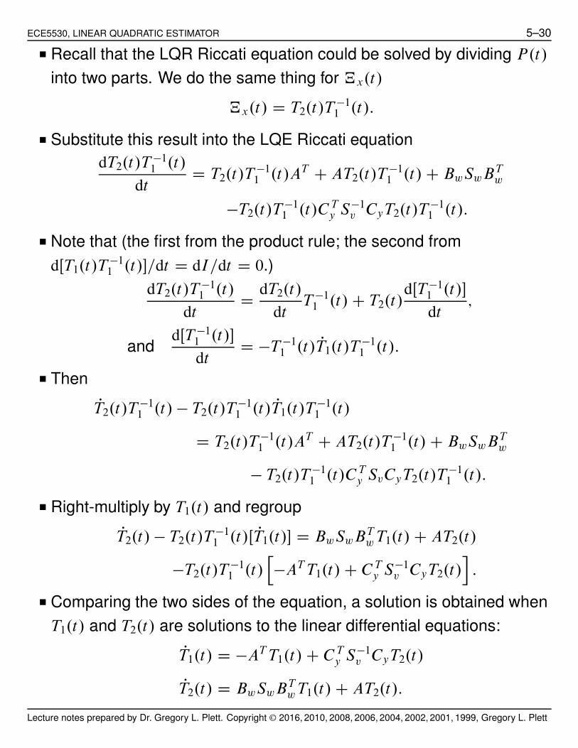
ECE5530, LINEAR QUADRATIC ESTIMATOR 5–30
■ Recall that the LQR Riccati equation could be solved by dividing P.t/
into two parts. We do the same thing for „x.t/
„x.t/ D T2.t/T"11 .t/:
■ Substitute this result into the LQE Riccati equation
dT2.t/T"11 .t/
dtD T2.t/T
"11 .t/AT C AT2.t/T
"11 .t/ C BwSwBT
w
"T2.t/T"11 .t/C T
y S"1v CyT2.t/T
"11 .t/:
■ Note that (the first from the product rule; the second from
dŒT1.t/T"11 .t/!=dt D dI=dt D 0.)
dT2.t/T"11 .t/
dtD
dT2.t/
dtT "1
1 .t/ C T2.t/dŒT "1
1 .t/!
dt;
anddŒT "1
1 .t/!
dtD "T "1
1 .t/ PT1.t/T"11 .t/:
■ Then
PT2.t/T"11 .t/ " T2.t/T
"11 .t/ PT1.t/T
"11 .t/
D T2.t/T"11 .t/AT C AT2.t/T
"11 .t/ C BwSwBT
w
" T2.t/T"11 .t/C T
y SvCyT2.t/T"11 .t/:
■ Right-multiply by T1.t/ and regroup
PT2.t/ " T2.t/T"11 .t/ΠPT1.t/! D BwSwBT
w T1.t/ C AT2.t/
"T2.t/T"11 .t/
h
"AT T1.t/ C C Ty S"1
v CyT2.t/i
:
■ Comparing the two sides of the equation, a solution is obtained when
T1.t/ and T2.t/ are solutions to the linear differential equations:
PT1.t/ D "AT T1.t/ C C Ty S"1
v CyT2.t/
PT2.t/ D BwSwBTw T1.t/ C AT2.t/:
Lecture notes prepared by Dr. Gregory L. Plett. Copyright © 2016, 2010, 2008, 2006, 2004, 2002, 2001, 1999, Gregory L. Plett

ECE5530, LINEAR QUADRATIC ESTIMATOR 5–31
■ Combining yields the Hamiltonian system for the Kalman filter"
PT1.t/
PT2.t/
#
D
"
"AT C Ty S"1
v Cy
BwSwBTw A
# "
T1.t/
T2.t/
#
D Y
"
T1.t/
T2.t/
#
■ The matrix Y is termed the Hamiltonian of the Kalman filter.
■ The initial conditions of the Hamiltonian system must satisfy
„x.0/ D T2.0/T "11 .0/;
so T1.0/ and T2.0/ are not uniquely specified. One choice is"
T1.0/
T2.0/
#
D
"
I
„x.0/
#
:
■ The Hamiltonian system is then solved as"
T1.t/
T2.t/
#
D eYt
"
I
„x.0/
#
D
"
ˆ11.t/ ˆ12.t/
ˆ21.t/ ˆ22.t/
# "
I
„x.0/
#
or
„x.t/ D fˆ21.t/ C ˆ22.t/„x.0/g fˆ11.t/ C ˆ12.t/„x.0/g"1
and the Kalman gain is
L.t/ D fˆ21.t/ C ˆ22.t/„x.0/g fˆ11.t/ C ˆ12.t/„x.0/g"1 C Ty S"1
v :
The steady-state Kalman gain
■ We can also use the Kalman Hamiltonian matrix to find the
steady-state gain matrix Lss much the same way we used the LQR
Hamiltonian matrix to find the steady-state matrix Kss.
■ The eigenequation of the Kalman Hamiltonian is"
"AT C Ty S"1
v Cy
BwSwBTw A
#
‰ D ‰ƒ:
Lecture notes prepared by Dr. Gregory L. Plett. Copyright © 2016, 2010, 2008, 2006, 2004, 2002, 2001, 1999, Gregory L. Plett

ECE5530, LINEAR QUADRATIC ESTIMATOR 5–32
■ Where ƒ is a diagonal matrix containing the eigenvalues of the
Hamiltonian (the first nx of which are in the left-half plane) and ‰ is
the matrix of eigenvectors. We can write ‰ as
‰ D
"
‰11 ‰12
‰21 ‰22
#
:
■ Using properties of the matrix exponential,"
T1.t/
T2.t/
#
D eYt
"
I
„x.0/
#
D e‰ƒ‰"1t
"
I
„x.0/
#
D ‰eƒt‰"1
"
I
„x.0/
#
D
"
‰11 ‰12
‰21 ‰22
# "
e"&t 0
0 e&t
#
‰"1
"
I
„x.0/
#
D
"
‰11e"&t ‰12e
&t
‰21e"&t ‰22e
&t
# "
.matrix top/
.matrix bottom/
#
:
■ As t ! 1, e"&t ! 0 and"
T1.t/
T2.t/
#
!
"
‰12
‰22
#
e&t .matrix bottom/:
■ The steady-state Riccati solution is then
„x;ss D T2.1/T "11 .1/
D ‰22.‰12/"1:
and the steady-state gain matrix is
Lss D ‰22.‰12/"1C T
y S"1v :
■ Note that the formula in the book is incorrect.
Lecture notes prepared by Dr. Gregory L. Plett. Copyright © 2016, 2010, 2008, 2006, 2004, 2002, 2001, 1999, Gregory L. Plett

ECE5530, LINEAR QUADRATIC ESTIMATOR 5–33
Appendix: Proof of matrix inversion lemma, form 2
■ Want to show!
NA"1 C NBT NC "1 NB""1 NBT NC "1 D NA NBT
!NB NA NBT C NC
""1:
■ Multiply on left by!
NA"1 C NBT NC "1 NB"
NBT NC "1 D!
NA"1 C NBT NC "1 NB"
NA NBT!
NB NA NBT C NC""1
D NBT!
NB NA NBT C NC""1
C NBT NC "1 NB NA NBT!
NB NA NBT C NC""1
D NBT˚
I C NC "1 NB NA NBT) !
NB NA NBT C NC""1
D NBT NC "1˚
NC C NB NA NBT) !
NB NA NBT C NC""1
D NBT NC "1:
Lecture notes prepared by Dr. Gregory L. Plett. Copyright © 2016, 2010, 2008, 2006, 2004, 2002, 2001, 1999, Gregory L. Plett