Linear Matrix Inequalities in System and Control Theoryboyd/lmibook/lmibook.pdf · Linear Matrix...
205
Linear Matrix Inequalities in System and Control Theory
Transcript of Linear Matrix Inequalities in System and Control Theoryboyd/lmibook/lmibook.pdf · Linear Matrix...

Linear Matrix Inequalities in
System and Control Theory

SIAM Studies in Applied Mathematics
This series of monographs focuses on mathematics and its applications to problemsof current concern to industry, government, and society. These monographs will be ofinterest to applied mathematicians, numerical analysts, statisticians, engineers, andscientists who have an active need to learn useful methodology.
Series List
Vol. 1 Lie-Backlund Transformations in ApplicationsRobert L. Anderson and Nail H. Ibragimov
Vol. 2 Methods and Applications of Interval AnalysisRamon E. Moore
Vol. 3 Ill-Posed Problems for Integrodifferential Equations in Mechanics andElectromagnetic TheoryFrederick Bloom
Vol. 4 Solitons and the Inverse Scattering TransformMark J. Ablowitz and Harvey Segur
Vol. 5 Fourier Analysis of Numerical Approximations of Hyperbolic EquationsRobert Vichnevetsky and John B. Bowles
Vol. 6 Numerical Solution of Elliptic ProblemsGarrett Birkhoff and Robert E. Lynch
Vol. 7 Analytical and Numerical Methods for Volterra EquationsPeter Linz
Vol. 8 Contact Problems in Elasticity: A Study of Variational Inequalities andFinite Element MethodsN. Kikuchi and J. T. Oden
Vol. 9 Augmented Lagrangian and Operator-Splitting Methods in NonlinearMechanicsRoland Glowinski and P. Le Tallec
Vol. 10 Boundary Stabilization of Thin Plate SplinesJohn E. Lagnese
Vol. 11 Electro-Diffusion of IonsIsaak Rubinstein
Vol. 12 Mathematical Problems in Linear ViscoelasticityMauro Fabrizio and Angelo Morro
Vol. 13 Interior-Point Polynomial Algorithms in Convex ProgrammingYurii Nesterov and Arkadii Nemirovskii
Vol. 14 The Boundary Function Method for Singular Perturbation ProblemsAdelaida B. Vasil’eva, Valentin F. Butuzov, and Leonid V. Kalachev
Vol. 15 Linear Matrix Inequalities in System and Control TheoryStephen Boyd, Laurent El Ghaoui, Eric Feron, and VenkataramananBalakrishnan

Stephen Boyd, Laurent El Ghaoui,
Eric Feron, and Venkataramanan Balakrishnan
Linear Matrix Inequalities in
System and Control Theory
Society for Industrial and Applied Mathematics
® Philadelphia
Copyright c© 1994 by the Society for Industrial and Applied Mathematics.
All rights reserved. No part of this book may be reproduced, stored, or transmitted in anymanner without the written permission of the Publisher. For information, write to the Societyfor Industrial and Applied Mathematics, 3600 University City Science Center, Philadelphia,Pennsylvania 19104-2688.
The royalties from the sales of this book are being placed in a fund to help studentsattend SIAM meetings and other SIAM related activities. This fund is administered bySIAM and qualified individuals are encouraged to write directly to SIAM for guidelines.
Library of Congress Cataloging-in-Publication Data
Linear matrix inequalities in system and control theory / Stephen Boyd. . . [et al.].
p. cm. -- (SIAM studies in applied mathematics ; vol. 15)Includes bibliographical references and index.ISBN 0-89871-334-X1. Control theory. 2. Matrix inequalities. 3. Mathematical
optimization. I. Boyd, Stephen P. II. Series: SIAM studies inapplied mathematics : 15.QA402.3.L489 1994515’.64--dc20 94-10477
Contents
Preface vii
Acknowledgments ix
1 Introduction 11.1 Overview . . . . . . . . . . . . . . . . . . . . . . . . . . . . . . . . . . 11.2 A Brief History of LMIs in Control Theory . . . . . . . . . . . . . . . 21.3 Notes on the Style of the Book . . . . . . . . . . . . . . . . . . . . . . 41.4 Origin of the Book . . . . . . . . . . . . . . . . . . . . . . . . . . . . . 5
2 Some Standard Problems Involving LMIs 72.1 Linear Matrix Inequalities . . . . . . . . . . . . . . . . . . . . . . . . . 72.2 Some Standard Problems . . . . . . . . . . . . . . . . . . . . . . . . . 92.3 Ellipsoid Algorithm . . . . . . . . . . . . . . . . . . . . . . . . . . . . . 122.4 Interior-Point Methods . . . . . . . . . . . . . . . . . . . . . . . . . . . 142.5 Strict and Nonstrict LMIs . . . . . . . . . . . . . . . . . . . . . . . . . 182.6 Miscellaneous Results on Matrix Inequalities . . . . . . . . . . . . . . 222.7 Some LMI Problems with Analytic Solutions . . . . . . . . . . . . . . 24Notes and References . . . . . . . . . . . . . . . . . . . . . . . . . . . . . . . 27
3 Some Matrix Problems 373.1 Minimizing Condition Number by Scaling . . . . . . . . . . . . . . . . 373.2 Minimizing Condition Number of a Positive-Definite Matrix . . . . . . 383.3 Minimizing Norm by Scaling . . . . . . . . . . . . . . . . . . . . . . . 383.4 Rescaling a Matrix Positive-Definite . . . . . . . . . . . . . . . . . . . 393.5 Matrix Completion Problems . . . . . . . . . . . . . . . . . . . . . . . 403.6 Quadratic Approximation of a Polytopic Norm . . . . . . . . . . . . . 413.7 Ellipsoidal Approximation . . . . . . . . . . . . . . . . . . . . . . . . . 42Notes and References . . . . . . . . . . . . . . . . . . . . . . . . . . . . . . . 47
4 Linear Differential Inclusions 514.1 Differential Inclusions . . . . . . . . . . . . . . . . . . . . . . . . . . . 514.2 Some Specific LDIs . . . . . . . . . . . . . . . . . . . . . . . . . . . . . 524.3 Nonlinear System Analysis via LDIs . . . . . . . . . . . . . . . . . . . 54Notes and References . . . . . . . . . . . . . . . . . . . . . . . . . . . . . . . 56
5 Analysis of LDIs: State Properties 615.1 Quadratic Stability . . . . . . . . . . . . . . . . . . . . . . . . . . . . . 615.2 Invariant Ellipsoids . . . . . . . . . . . . . . . . . . . . . . . . . . . . . 68
v
vi Contents
Notes and References . . . . . . . . . . . . . . . . . . . . . . . . . . . . . . . 72
6 Analysis of LDIs: Input/Output Properties 776.1 Input-to-State Properties . . . . . . . . . . . . . . . . . . . . . . . . . 776.2 State-to-Output Properties . . . . . . . . . . . . . . . . . . . . . . . . 846.3 Input-to-Output Properties . . . . . . . . . . . . . . . . . . . . . . . . 89Notes and References . . . . . . . . . . . . . . . . . . . . . . . . . . . . . . . 96
7 State-Feedback Synthesis for LDIs 997.1 Static State-Feedback Controllers . . . . . . . . . . . . . . . . . . . . . 997.2 State Properties . . . . . . . . . . . . . . . . . . . . . . . . . . . . . . 1007.3 Input-to-State Properties . . . . . . . . . . . . . . . . . . . . . . . . . 1047.4 State-to-Output Properties . . . . . . . . . . . . . . . . . . . . . . . . 1077.5 Input-to-Output Properties . . . . . . . . . . . . . . . . . . . . . . . . 1097.6 Observer-Based Controllers for Nonlinear Systems . . . . . . . . . . . 111Notes and References . . . . . . . . . . . . . . . . . . . . . . . . . . . . . . . 112
8 Lur’e and Multiplier Methods 1198.1 Analysis of Lur’e Systems . . . . . . . . . . . . . . . . . . . . . . . . . 1198.2 Integral Quadratic Constraints . . . . . . . . . . . . . . . . . . . . . . 1228.3 Multipliers for Systems with Unknown Parameters . . . . . . . . . . . 124Notes and References . . . . . . . . . . . . . . . . . . . . . . . . . . . . . . . 126
9 Systems with Multiplicative Noise 1319.1 Analysis of Systems with Multiplicative Noise . . . . . . . . . . . . . . 1319.2 State-Feedback Synthesis . . . . . . . . . . . . . . . . . . . . . . . . . 134Notes and References . . . . . . . . . . . . . . . . . . . . . . . . . . . . . . . 136
10 Miscellaneous Problems 14110.1 Optimization over an Affine Family of Linear Systems . . . . . . . . . 14110.2 Analysis of Systems with LTI Perturbations . . . . . . . . . . . . . . . 14310.3 Positive Orthant Stabilizability . . . . . . . . . . . . . . . . . . . . . . 14410.4 Linear Systems with Delays . . . . . . . . . . . . . . . . . . . . . . . . 14410.5 Interpolation Problems . . . . . . . . . . . . . . . . . . . . . . . . . . . 14510.6 The Inverse Problem of Optimal Control . . . . . . . . . . . . . . . . . 14710.7 System Realization Problems . . . . . . . . . . . . . . . . . . . . . . . 14810.8 Multi-Criterion LQG . . . . . . . . . . . . . . . . . . . . . . . . . . . . 15010.9 Nonconvex Multi-Criterion Quadratic Problems . . . . . . . . . . . . . 151Notes and References . . . . . . . . . . . . . . . . . . . . . . . . . . . . . . . 152
Notation 157
List of Acronyms 159
Bibliography 161
Index 187
Copyright c© 1994 by the Society for Industrial and Applied Mathematics.

Preface
The basic topic of this book is solving problems from system and control theory usingconvex optimization. We show that a wide variety of problems arising in systemand control theory can be reduced to a handful of standard convex and quasiconvexoptimization problems that involve matrix inequalities. For a few special cases thereare “analytic solutions” to these problems, but our main point is that they can besolved numerically in all cases. These standard problems can be solved in polynomial-time (by, e.g., the ellipsoid algorithm of Shor, Nemirovskii, and Yudin), and so aretractable, at least in a theoretical sense. Recently developed interior-point methodsfor these standard problems have been found to be extremely efficient in practice.Therefore, we consider the original problems from system and control theory as solved.
This book is primarily intended for the researcher in system and control theory,but can also serve as a source of application problems for researchers in convex op-timization. Although we believe that the methods described in this book have greatpractical value, we should warn the reader whose primary interest is applied controlengineering. This is a research monograph: We present no specific examples or nu-merical results, and we make only brief comments about the implications of the resultsfor practical control engineering. To put it in a more positive light, we hope that thisbook will later be considered as the first book on the topic, not the most readable oraccessible.
The background required of the reader is knowledge of basic system and controltheory and an exposure to optimization. Sontag’s book Mathematical Control The-
ory [Son90] is an excellent survey. Further background material is covered in thetexts Linear Systems [Kai80] by Kailath, Nonlinear Systems Analysis [Vid92] byVidyasagar, Optimal Control: Linear Quadratic Methods [AM90] by Anderson andMoore, and Convex Analysis and Minimization Algorithms I [HUL93] by Hiriart–Urruty and Lemarechal.
We also highly recommend the book Interior-point Polynomial Algorithms in Con-
vex Programming [NN94] by Nesterov and Nemirovskii as a companion to this book.The reader will soon see that their ideas and methods play a critical role in the basicidea presented in this book.
vii

Acknowledgments
We thank A. Nemirovskii for encouraging us to write this book. We are grateful to S.Hall, M. Gevers, and A. Packard for introducing us to multiplier methods, realizationtheory, and state-feedback synthesis methods, respectively. This book was greatlyimproved by the suggestions of J. Abedor, P. Dankoski, J. Doyle, G. Franklin, T.Kailath, R. Kosut, I. Petersen, E. Pyatnitskii, M. Rotea, M. Safonov, S. Savastiouk,A. Tits, L. Vandenberghe, and J. C. Willems. It is a special pleasure to thank V.Yakubovich for his comments and suggestions.
The research reported in this book was supported in part by AFOSR (underF49620-92-J-0013), NSF (under ECS-9222391), and ARPA (under F49620-93-1-0085).L. El Ghaoui and E. Feron were supported in part by the Delegation Generale pourl’Armement. E. Feron was supported in part by the Charles Stark Draper CareerDevelopment Chair at MIT. V. Balakrishnan was supported in part by the Controland Dynamical Systems Group at Caltech and by NSF (under NSFD CDR-8803012).
This book was typeset by the authors using LATEX, and many macros originallywritten by Craig Barratt.
Stephen Boyd Stanford, California
Laurent El Ghaoui Paris, France
Eric Feron Cambridge, Massachusetts
Venkataramanan Balakrishnan College Park, Maryland
ix

Linear Matrix Inequalities in
System and Control Theory

Chapter 1
Introduction
1.1 Overview
The aim of this book is to show that we can reduce a very wide variety of prob-lems arising in system and control theory to a few standard convex or quasiconvexoptimization problems involving linear matrix inequalities (LMIs). Since these result-ing optimization problems can be solved numerically very efficiently using recentlydeveloped interior-point methods, our reduction constitutes a solution to the originalproblem, certainly in a practical sense, but also in several other senses as well. In com-parison, the more conventional approach is to seek an analytic or frequency-domainsolution to the matrix inequalities.
The types of problems we consider include:
• matrix scaling problems, e.g., minimizing condition number by diagonal scaling
• construction of quadratic Lyapunov functions for stability and performance anal-ysis of linear differential inclusions
• joint synthesis of state-feedback and quadratic Lyapunov functions for lineardifferential inclusions
• synthesis of state-feedback and quadratic Lyapunov functions for stochastic anddelay systems
• synthesis of Lur’e-type Lyapunov functions for nonlinear systems
• optimization over an affine family of transfer matrices, including synthesis ofmultipliers for analysis of linear systems with unknown parameters
• positive orthant stability and state-feedback synthesis
• optimal system realization
• interpolation problems, including scaling
• multicriterion LQG/LQR
• inverse problem of optimal control
In some cases, we are describing known, published results; in others, we are extendingknown results. In many cases, however, it seems that the results are new.
By scanning the list above or the table of contents, the reader will see that Lya-punov’s methods will be our main focus. Here we have a secondary goal, beyondshowing that many problems from Lyapunov theory can be cast as convex or quasi-convex problems. This is to show that Lyapunov’s methods, which are traditionally
1
2 Chapter 1 Introduction
applied to the analysis of system stability , can just as well be used to find bounds onsystem performance, provided we do not insist on an “analytic solution”.
1.2 A Brief History of LMIs in Control Theory
The history of LMIs in the analysis of dynamical systems goes back more than 100years. The story begins in about 1890, when Lyapunov published his seminal workintroducing what we now call Lyapunov theory. He showed that the differential equa-tion
d
dtx(t) = Ax(t) (1.1)
is stable (i.e., all trajectories converge to zero) if and only if there exists a positive-definite matrix P such that
ATP + PA < 0. (1.2)
The requirement P > 0, ATP +PA < 0 is what we now call a Lyapunov inequality onP , which is a special form of an LMI. Lyapunov also showed that this first LMI couldbe explicitly solved. Indeed, we can pick any Q = QT > 0 and then solve the linearequation ATP+PA = −Q for the matrix P , which is guaranteed to be positive-definiteif the system (1.1) is stable. In summary, the first LMI used to analyze stability of adynamical system was the Lyapunov inequality (1.2), which can be solved analytically(by solving a set of linear equations).
The next major milestone occurs in the 1940’s. Lur’e, Postnikov, and others inthe Soviet Union applied Lyapunov’s methods to some specific practical problemsin control engineering, especially, the problem of stability of a control system with anonlinearity in the actuator. Although they did not explicitly form matrix inequalities,their stability criteria have the form of LMIs. These inequalities were reduced topolynomial inequalities which were then checked “by hand” (for, needless to say, smallsystems). Nevertheless they were justifiably excited by the idea that Lyapunov’stheory could be applied to important (and difficult) practical problems in controlengineering. From the introduction of Lur’e’s 1951 book [Lur57] we find:
This book represents the first attempt to demonstrate that the ideas ex-pressed 60 years ago by Lyapunov, which even comparatively recently ap-peared to be remote from practical application, are now about to become areal medium for the examination of the urgent problems of contemporaryengineering.
In summary, Lur’e and others were the first to apply Lyapunov’s methods to practicalcontrol engineering problems. The LMIs that resulted were solved analytically, byhand. Of course this limited their application to small (second, third order) systems.
The next major breakthrough came in the early 1960’s, when Yakubovich, Popov,Kalman, and other researchers succeeded in reducing the solution of the LMIs thatarose in the problem of Lur’e to simple graphical criteria, using what we now callthe positive-real (PR) lemma (see §2.7.2). This resulted in the celebrated Popovcriterion, circle criterion, Tsypkin criterion, and many variations. These criteria couldbe applied to higher order systems, but did not gracefully or usefully extend to systemscontaining more than one nonlinearity. From the point of view of our story (LMIs incontrol theory), the contribution was to show how to solve a certain family of LMIsby graphical methods.
Copyright c© 1994 by the Society for Industrial and Applied Mathematics.
1.2 A Brief History of LMIs in Control Theory 3
The important role of LMIs in control theory was already recognized in the early1960’s, especially by Yakubovich [Yak62, Yak64, Yak67]. This is clear simply fromthe titles of some of his papers from 1962–5, e.g., The solution of certain matrix
inequalities in automatic control theory (1962), and The method of matrix inequalities
in the stability theory of nonlinear control systems (1965; English translation 1967).The PR lemma and extensions were intensively studied in the latter half of the
1960s, and were found to be related to the ideas of passivity, the small-gain criteriaintroduced by Zames and Sandberg, and quadratic optimal control. By 1970, it wasknown that the LMI appearing in the PR lemma could be solved not only by graphicalmeans, but also by solving a certain algebraic Riccati equation (ARE). In a 1971paper [Wil71b] on quadratic optimal control, J. C. Willems is led to the LMI
[
ATP + PA+Q PB + CT
BTP + C R
]
≥ 0, (1.3)
and points out that it can be solved by studying the symmetric solutions of the ARE
ATP + PA− (PB + CT )R−1(BTP + C) +Q = 0,
which in turn can be found by an eigendecomposition of a related Hamiltonian matrix.(See §2.7.2 for details.) This connection had been observed earlier in the Soviet Union,where the ARE was called the Lur’e resolving equation (see [Yak88]).
So by 1971, researchers knew several methods for solving special types of LMIs:direct (for small systems), graphical methods, and by solving Lyapunov or Riccatiequations. From our point of view, these methods are all “closed-form” or “analytic”solutions that can be used to solve special forms of LMIs. (Most control researchersand engineers consider the Riccati equation to have an “analytic” solution, since thestandard algorithms that solve it are very predictable in terms of the effort required,which depends almost entirely on the problem size and not the particular problemdata. Of course it cannot be solved exactly in a finite number of arithmetic steps forsystems of fifth and higher order.)
In Willems’ 1971 paper we find the following striking quote:
The basic importance of the LMI seems to be largely unappreciated. Itwould be interesting to see whether or not it can be exploited in compu-tational algorithms, for example.
Here Willems refers to the specific LMI (1.3), and not the more general form thatwe consider in this book. Still, Willems’ suggestion that LMIs might have someadvantages in computational algorithms (as compared to the corresponding Riccatiequations) foreshadows the next chapter in the story.
The next major advance (in our view) was the simple observation that:
The LMIs that arise in system and control theory can be formulated asconvex optimization problems that are amenable to computer solution.
Although this is a simple observation, it has some important consequences, the mostimportant of which is that we can reliably solve many LMIs for which no “analyticsolution” has been found (or is likely to be found).
This observation was made explicitly by several researchers. Pyatnitskii and Sko-rodinskii [PS82] were perhaps the first researchers to make this point, clearly andcompletely. They reduced the original problem of Lur’e (extended to the case of mul-tiple nonlinearities) to a convex optimization problem involving LMIs, which they
This electronic version is for personal use and may not be duplicated or distributed.
4 Chapter 1 Introduction
then solved using the ellipsoid algorithm. (This problem had been studied before, butthe “solutions” involved an arbitrary scaling matrix.) Pyatnitskii and Skorodinskiiwere the first, as far as we know, to formulate the search for a Lyapunov function asa convex optimization problem, and then apply an algorithm guaranteed to solve theoptimization problem.
We should also mention several precursors. In a 1976 paper, Horisberger and Be-langer [HB76] had remarked that the existence of a quadratic Lyapunov function thatsimultaneously proves stability of a collection of linear systems is a convex probleminvolving LMIs. And of course, the idea of having a computer search for a Lya-punov function was not new—it appears, for example, in a 1965 paper by Schultz etal. [SSHJ65].
The final chapter in our story is quite recent and of great practical importance: thedevelopment of powerful and efficient interior-point methods to solve the LMIs thatarise in system and control theory. In 1984, N. Karmarkar introduced a new linearprogramming algorithm that solves linear programs in polynomial-time, like the ellip-soid method, but in contrast to the ellipsoid method, is also very efficient in practice.Karmarkar’s work spurred an enormous amount of work in the area of interior-pointmethods for linear programming (including the rediscovery of efficient methods thatwere developed in the 1960s but ignored). Essentially all of this research activity con-centrated on algorithms for linear and (convex) quadratic programs. Then in 1988,Nesterov and Nemirovskii developed interior-point methods that apply directly to con-vex problems involving LMIs, and in particular, to the problems we encounter in thisbook. Although there remains much to be done in this area, several interior-pointalgorithms for LMI problems have been implemented and tested on specific familiesof LMIs that arise in control theory, and found to be extremely efficient.
A summary of key events in the history of LMIs in control theory is then:
• 1890: First LMI appears; analytic solution of the Lyapunov LMI via Lyapunovequation.
• 1940’s: Application of Lyapunov’s methods to real control engineering prob-lems. Small LMIs solved “by hand”.
• Early 1960’s: PR lemma gives graphical techniques for solving another familyof LMIs.
• Late 1960’s: Observation that the same family of LMIs can be solved by solvingan ARE.
• Early 1980’s: Recognition that many LMIs can be solved by computer viaconvex programming.
• Late 1980’s: Development of interior-point algorithms for LMIs.
It is fair to say that Yakubovich is the father of the field, and Lyapunov the grandfatherof the field. The new development is the ability to directly solve (general) LMIs.
1.3 Notes on the Style of the Book
We use a very informal mathematical style, e.g., we often fail to mention regularity orother technical conditions. Every statement is to be interpreted as being true moduloappropriate technical conditions (that in most cases are trivial to figure out).
We are very informal, perhaps even cavalier, in our reduction of a problem toan optimization problem. We sometimes skip “details” that would be important ifthe optimization problem were to be solved numerically. As an example, it may be
Copyright c© 1994 by the Society for Industrial and Applied Mathematics.
1.4 Origin of the Book 5
necessary to add constraints to the optimization problem for normalization or to ensureboundedness. We do not discuss initial guesses for the optimization problems, eventhough good ones may be available. Therefore, the reader who wishes to implement
an algorithm that solves a problem considered in this book should be prepared tomake a few modifications or additions to our description of the “solution”.
In a similar way, we do not pursue any theoretical aspects of reducing a problemto a convex problem involving matrix inequalities. For example, for each reducedproblem we could state, probably simplify, and then interpret in system or controltheoretic terms the optimality conditions for the resulting convex problem. Anotherfascinating topic that could be explored is the relation between system and controltheory duality and convex programming duality. Once we reduce a problem arisingin control theory to a convex program, we can consider various dual optimizationproblems, lower bounds for the problem, and so on. Presumably these dual problemsand lower bounds can be given interesting system-theoretic interpretations.
We mostly consider continuous-time systems, and assume that the reader cantranslate the results from the continuous-time case to the discrete-time case. Weswitch to discrete-time systems when we consider system realization problems (whichalmost always arise in this form) and also when we consider stochastic systems (toavoid the technical details of stochastic differential equations).
The list of problems that we consider is meant only to be representative, andcertainly not exhaustive. To avoid excessive repetition, our treatment of problemsbecomes more terse as the book progresses. In the first chapter on analysis of lin-ear differential inclusions, we describe many variations on problems (e.g., computingbounds on margins and decay rates); in later chapters, we describe fewer and fewervariations, assuming that the reader could work out the extensions.
Each chapter concludes with a section entitled Notes and References, in which wehide proofs, precise statements, elaborations, and bibliography and historical notes.The completeness of the bibliography should not be overestimated, despite its size(over 500 entries). The appendix contains a list of notation and a list of acronymsused in the book. We apologize to the reader for the seven new acronyms we introduce.
To lighten the notation, we use the standard convention of dropping the timeargument from the variables in differential equations. Thus, x = Ax is our shortform for dx/dt = Ax(t). Here A is a constant matrix; when we encounter time-varying coefficients, we will explicitly show the time dependence, as in x = A(t)x.Similarly, we drop the dummy variable from definite integrals, writing for example,∫ T
0uT ydt for
∫ T
0u(t)T y(t)dt. To reduce the number of parentheses required, we adopt
the convention that the operators Tr (trace of a matrix) and E (expected value) havelower precedence than multiplication, transpose, etc. Thus, TrATB means Tr
(
ATB)
.
1.4 Origin of the Book
This book started out as a section of the paper Method of Centers for Minimizing
Generalized Eigenvalues, by Boyd and El Ghaoui [BE93], but grew too large to bea section. For a few months it was a manuscript (that presumably would have beensubmitted for publication as a paper) entitled Generalized Eigenvalue Problems Aris-
ing in Control Theory. Then Feron, and later Balakrishnan, started adding material,and soon it was clear that we were writing a book, not a paper. The order of theauthors’ names reflects this history.
This electronic version is for personal use and may not be duplicated or distributed.

Chapter 2
Some Standard ProblemsInvolving LMIs
2.1 Linear Matrix Inequalities
A linear matrix inequality (LMI) has the form
F (x)∆= F0 +
m∑
i=1
xiFi > 0, (2.1)
where x ∈ Rm is the variable and the symmetric matrices Fi = FTi ∈ Rn×n, i =
0, . . . ,m, are given. The inequality symbol in (2.1) means that F (x) is positive-definite, i.e., uTF (x)u > 0 for all nonzero u ∈ Rn. Of course, the LMI (2.1) isequivalent to a set of n polynomial inequalities in x, i.e., the leading principal minorsof F (x) must be positive.
We will also encounter nonstrict LMIs, which have the form
F (x) ≥ 0. (2.2)
The strict LMI (2.1) and the nonstrict LMI (2.2) are closely related, but a precisestatement of the relation is a bit involved, so we defer it to §2.5. In the next fewsections we consider strict LMIs.
The LMI (2.1) is a convex constraint on x, i.e., the set x | F (x) > 0 is convex.Although the LMI (2.1) may seem to have a specialized form, it can represent awide variety of convex constraints on x. In particular, linear inequalities, (convex)quadratic inequalities, matrix norm inequalities, and constraints that arise in controltheory, such as Lyapunov and convex quadratic matrix inequalities, can all be cast inthe form of an LMI.
Multiple LMIs F (1)(x) > 0, . . . , F (p)(x) > 0 can be expressed as the single LMIdiag(F (1)(x), . . . , F (p)(x)) > 0. Therefore we will make no distinction between a setof LMIs and a single LMI, i.e., “the LMI F (1)(x) > 0, . . . , F (p)(x) > 0” will mean “theLMI diag(F (1)(x), . . . , F (p)(x)) > 0”.
When the matrices Fi are diagonal, the LMI F (x) > 0 is just a set of linearinequalities. Nonlinear (convex) inequalities are converted to LMI form using Schurcomplements. The basic idea is as follows: the LMI
[
Q(x) S(x)
S(x)T R(x)
]
> 0, (2.3)
7
8 Chapter 2 Some Standard Problems Involving LMIs
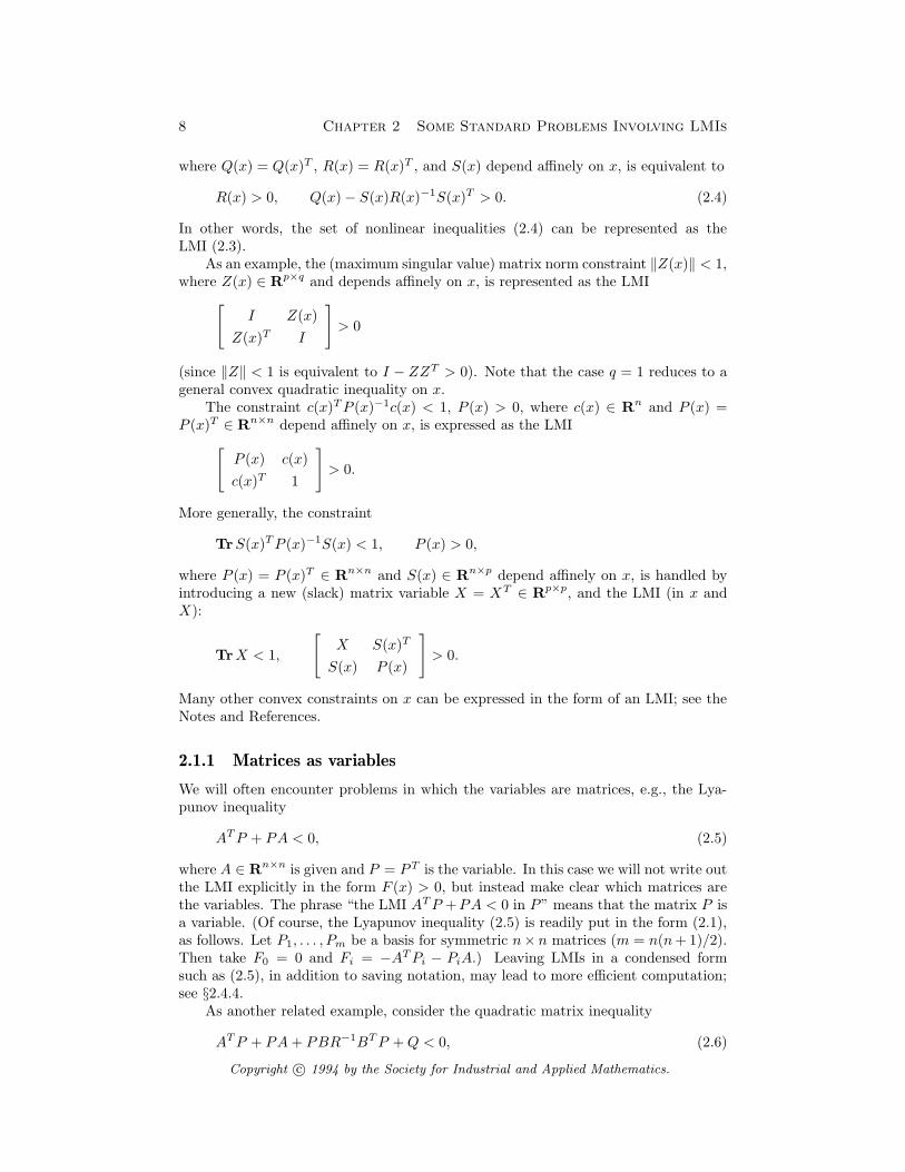
where Q(x) = Q(x)T , R(x) = R(x)T , and S(x) depend affinely on x, is equivalent to
R(x) > 0, Q(x)− S(x)R(x)−1S(x)T > 0. (2.4)
In other words, the set of nonlinear inequalities (2.4) can be represented as theLMI (2.3).
As an example, the (maximum singular value) matrix norm constraint ‖Z(x)‖ < 1,where Z(x) ∈ Rp×q and depends affinely on x, is represented as the LMI
[
I Z(x)
Z(x)T I
]
> 0
(since ‖Z‖ < 1 is equivalent to I − ZZT > 0). Note that the case q = 1 reduces to ageneral convex quadratic inequality on x.
The constraint c(x)TP (x)−1c(x) < 1, P (x) > 0, where c(x) ∈ Rn and P (x) =P (x)T ∈ Rn×n depend affinely on x, is expressed as the LMI
[
P (x) c(x)
c(x)T 1
]
> 0.
More generally, the constraint
TrS(x)TP (x)−1S(x) < 1, P (x) > 0,
where P (x) = P (x)T ∈ Rn×n and S(x) ∈ Rn×p depend affinely on x, is handled byintroducing a new (slack) matrix variable X = XT ∈ Rp×p, and the LMI (in x andX):
TrX < 1,
[
X S(x)T
S(x) P (x)
]
> 0.
Many other convex constraints on x can be expressed in the form of an LMI; see theNotes and References.
2.1.1 Matrices as variables
We will often encounter problems in which the variables are matrices, e.g., the Lya-punov inequality
ATP + PA < 0, (2.5)
where A ∈ Rn×n is given and P = P T is the variable. In this case we will not write outthe LMI explicitly in the form F (x) > 0, but instead make clear which matrices arethe variables. The phrase “the LMI ATP +PA < 0 in P” means that the matrix P isa variable. (Of course, the Lyapunov inequality (2.5) is readily put in the form (2.1),as follows. Let P1, . . . , Pm be a basis for symmetric n× n matrices (m = n(n+1)/2).Then take F0 = 0 and Fi = −ATPi − PiA.) Leaving LMIs in a condensed formsuch as (2.5), in addition to saving notation, may lead to more efficient computation;see §2.4.4.
As another related example, consider the quadratic matrix inequality
ATP + PA+ PBR−1BTP +Q < 0, (2.6)
Copyright c© 1994 by the Society for Industrial and Applied Mathematics.

2.2 Some Standard Problems 9
where A, B, Q = QT , R = RT > 0 are given matrices of appropriate sizes, andP = PT is the variable. Note that this is a quadratic matrix inequality in the variableP . It can be expressed as the linear matrix inequality
[
−ATP − PA−Q PB
BTP R
]
> 0.
This representation also clearly shows that the quadratic matrix inequality (2.6) isconvex in P , which is not obvious.
2.1.2 Linear equality constraints
In some problems we will encounter linear equality constraints on the variables, e.g.
P > 0, ATP + PA < 0, TrP = 1, (2.7)
where P ∈ Rk×k is the variable. Of course we can eliminate the equality constraint towrite (2.7) in the form F (x) > 0. Let P1, . . . , Pm be a basis for symmetric k×k matriceswith trace zero (m = (k(k + 1)/2)− 1) and let P0 be a symmetric k × k matrix withTrP0 = 1. Then take F0 = diag(P0,−ATP0−P0A) and Fi = diag(Pi,−ATPi−PiA)for i = 1, . . . ,m.
We will refer to constraints such as (2.7) as LMIs, leaving any required eliminationof equality constraints to the reader.
2.2 Some Standard Problems
Here we list some common convex and quasiconvex problems that we will encounterin the sequel.
2.2.1 LMI problems
Given an LMI F (x) > 0, the corresponding LMI Problem (LMIP) is to find xfeas suchthat F (xfeas) > 0 or determine that the LMI is infeasible. (By duality, this means:Find a nonzero G ≥ 0 such that TrGFi = 0 for i = 1, . . . ,m and TrGF0 ≤ 0; see theNotes and References.) Of course, this is a convex feasibility problem. We will say“solving the LMI F (x) > 0” to mean solving the corresponding LMIP.
As an example of an LMIP, consider the “simultaneous Lyapunov stability prob-lem” (which we will see in §5.1): We are given Ai ∈ Rn×n, i = 1, . . . , L, and need tofind P satisfying the LMI
P > 0, ATi P + PAi < 0, i = 1, . . . , L,
or determine that no such P exists. Determining that no such P exists is equivalentto finding Q0, . . . , QL, not all zero, such that
Q0 ≥ 0, . . . , QL ≥ 0, Q0 =L∑
i=1
(
QiATi +AiQi
)
, (2.8)
which is another (nonstrict) LMIP.
This electronic version is for personal use and may not be duplicated or distributed.
10 Chapter 2 Some Standard Problems Involving LMIs
2.2.2 Eigenvalue problems
The eigenvalue problem (EVP) is to minimize the maximum eigenvalue of a matrixthat depends affinely on a variable, subject to an LMI constraint (or determine thatthe constraint is infeasible), i.e.,
minimize λ
subject to λI −A(x) > 0, B(x) > 0
where A and B are symmetric matrices that depend affinely on the optimizationvariable x. This is a convex optimization problem.
EVPs can appear in the equivalent form of minimizing a linear function subjectto an LMI, i.e.,
minimize cTx
subject to F (x) > 0(2.9)
with F an affine function of x. In the special case when the matrices Fi are all diagonal,this problem reduces to the general linear programming problem: minimizing thelinear function cTx subject to a set of linear inequalities on x.
Another equivalent form for the EVP is:
minimize λ
subject to A(x, λ) > 0
where A is affine in (x, λ). We leave it to the reader to verify that these forms areequivalent, i.e., any can be transformed into any other.
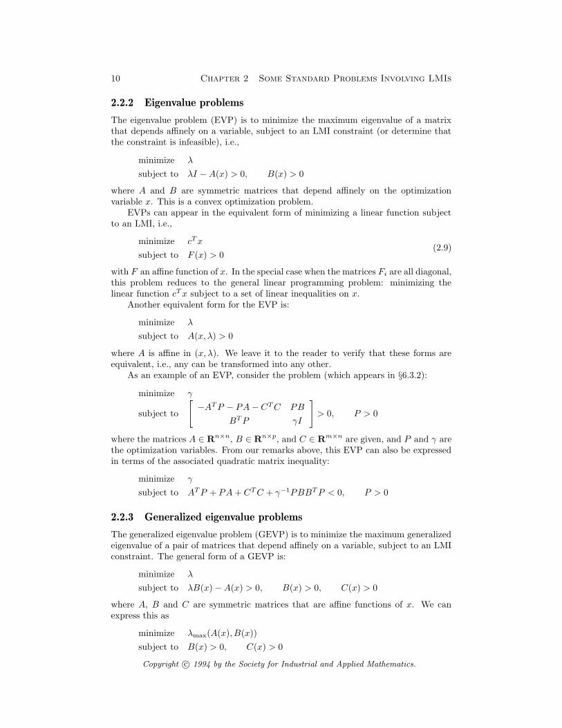
As an example of an EVP, consider the problem (which appears in §6.3.2):
minimize γ
subject to
[
−ATP − PA− CTC PB
BTP γI
]
> 0, P > 0
where the matrices A ∈ Rn×n, B ∈ Rn×p, and C ∈ Rm×n are given, and P and γ arethe optimization variables. From our remarks above, this EVP can also be expressedin terms of the associated quadratic matrix inequality:
minimize γ
subject to ATP + PA+ CTC + γ−1PBBTP < 0, P > 0
2.2.3 Generalized eigenvalue problems
The generalized eigenvalue problem (GEVP) is to minimize the maximum generalizedeigenvalue of a pair of matrices that depend affinely on a variable, subject to an LMIconstraint. The general form of a GEVP is:
minimize λ
subject to λB(x)−A(x) > 0, B(x) > 0, C(x) > 0
where A, B and C are symmetric matrices that are affine functions of x. We canexpress this as
minimize λmax(A(x), B(x))
subject to B(x) > 0, C(x) > 0
Copyright c© 1994 by the Society for Industrial and Applied Mathematics.
2.2 Some Standard Problems 11
where λmax(X,Y ) denotes the largest generalized eigenvalue of the pencil λY − Xwith Y > 0, i.e., the largest eigenvalue of the matrix Y −1/2XY −1/2. This GEVP isa quasiconvex optimization problem since the constraint is convex and the objective,λmax(A(x), B(x)), is quasiconvex. This means that for feasible x, x and 0 ≤ θ ≤ 1,
λmax(A(θx+ (1− θ)x), B(θx+ (1− θ)x)) ≤max λmax(A(x), B(x)), λmax(A(x), B(x)) .
Note that when the matrices are all diagonal and A(x) and B(x) are scalar, thisproblem reduces to the general linear-fractional programming problem, i.e., minimiz-ing a linear-fractional function subject to a set of linear inequalities. In addition,many nonlinear quasiconvex functions can be represented in the form of a GEVP withappropriate A, B, and C; see the Notes and References.
An equivalent alternate form for a GEVP is
minimize λ
subject to A(x, λ) > 0
where A(x, λ) is affine in x for fixed λ and affine in λ for fixed x, and satisfies themonotonicity condition λ > µ =⇒ A(x, λ) ≥ A(x, µ). As an example of a GEVP,consider the problem
maximize α
subject to −ATP − PA− 2αP > 0, P > 0
where the matrix A is given, and the optimization variables are the symmetric matrixP and the scalar α. (This problem arises in §5.1.)
2.2.4 A convex problem
Although we will be concerned mostly with LMIPs, EVPs, and GEVPs, we will alsoencounter the following convex problem, which we will abbreviate CP:
minimize log detA(x)−1
subject to A(x) > 0, B(x) > 0(2.10)
where A and B are symmetric matrices that depend affinely on x. (Note that whenA > 0, log detA−1 is a convex function of A.)
Remark: Problem CP can be transformed into an EVP, since detA(x) > λ canbe represented as an LMI in x and λ; see [NN94, §6.4.3]. As we do with variableswhich are matrices, we leave these problems in the more natural form.
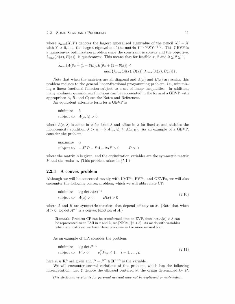
As an example of CP, consider the problem:
minimize log detP−1
subject to P > 0, vTi Pvi ≤ 1, i = 1, . . . , L(2.11)
here vi ∈ Rn are given and P = P T ∈ Rn×n is the variable.We will encounter several variations of this problem, which has the following
interpretation. Let E denote the ellipsoid centered at the origin determined by P ,
This electronic version is for personal use and may not be duplicated or distributed.
12 Chapter 2 Some Standard Problems Involving LMIs
E ∆=
z∣
∣ zTPz ≤ 1
. The constraints are simply vi ∈ E . Since the volume of E is pro-
portional to (detP )−1/2, minimizing log detP−1 is the same as minimizing the volumeof E . So by solving (2.11), we find the minimum volume ellipsoid, centered at the ori-gin, that contains the points v1, . . . , vL, or equivalently, the polytope Cov1, . . . , vL,where Co denotes the convex hull.
2.2.5 Solving these problems
The standard problems (LMIPs, EVPs, GEVPs, and CPs) are tractable, from boththeoretical and practical viewpoints:
• They can be solved in polynomial-time (indeed with a variety of interpretationsfor the term “polynomial-time”).
• They can be solved in practice very efficiently.
By “solve the problem” we mean: Determine whether or not the problem is fea-sible, and if it is, compute a feasible point with an objective value that exceeds theglobal minimum by less than some prespecified accuracy.
2.3 Ellipsoid Algorithm
We first describe a simple ellipsoid algorithm that, roughly speaking, is guaranteedto solve the standard problems. We describe it here because it is very simple and,from a theoretical point of view, efficient (polynomial-time). In practice, however, theinterior-point algorithms described in the next section are much more efficient.
Although more sophisticated versions of the ellipsoid algorithm can detect in-feasible constraints, we will assume that the problem we are solving has at least oneoptimal point, i.e., the constraints are feasible. (In the feasibility problem, we considerany feasible point as being optimal.) The basic idea of the algorithm is as follows. Westart with an ellipsoid E (0) that is guaranteed to contain an optimal point. We thencompute a cutting plane for our problem that passes through the center x(0) of E(0).This means that we find a nonzero vector g(0) such that an optimal point lies in thehalf-space
z∣
∣ g(0)T (z − x(0)) ≤ 0
(or in the half-space
z∣
∣ g(0)T (z − x(0)) < 0
,depending on the situation). (We will explain how to do this for each of our problemslater.) We then know that the sliced half-ellipsoid
E(0) ∩
z∣
∣
∣ g(0)T (z − x(0)) ≤ 0
contains an optimal point. Now we compute the ellipsoid E (1) of minimum volumethat contains this sliced half-ellipsoid; E (1) is then guaranteed to contain an optimalpoint. The process is then repeated.
We now describe the algorithm more explicitly. An ellipsoid E can be describedas
E =
z∣
∣ (z − a)TA−1(z − a) ≤ 1
where A = AT > 0. The minimum volume ellipsoid that contains the half-ellipsoid
z∣
∣ (z − a)TA−1(z − a) ≤ 1, gT (z − a) ≤ 0
is given by
E =
z∣
∣
∣ (z − a)T A−1(z − a) ≤ 1
,
Copyright c© 1994 by the Society for Industrial and Applied Mathematics.
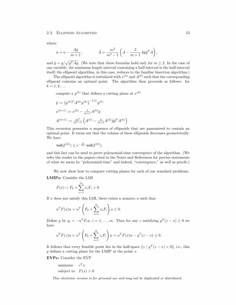
2.3 Ellipsoid Algorithm 13
where
a = a− Ag
m+ 1, A =
m2
m2 − 1
(
A− 2
m+ 1AggTA
)
,
and g = g/√
gTAg. (We note that these formulas hold only for m ≥ 2. In the case ofone variable, the minimum length interval containing a half-interval is the half-intervalitself; the ellipsoid algorithm, in this case, reduces to the familiar bisection algorithm.)
The ellipsoid algorithm is initialized with x(0) andA(0) such that the correspondingellipsoid contains an optimal point. The algorithm then proceeds as follows: fork = 1, 2, . . .
compute a g(k) that defines a cutting plane at x(k)
g :=(
g(k)TA(k)g(k))−1/2
g(k)
x(k+1) := x(k) − 1m+1A
(k)g
A(k+1) := m2
m2−1
(
A(k) − 2m+1A
(k)ggTA(k))
This recursion generates a sequence of ellipsoids that are guaranteed to contain anoptimal point. It turns out that the volume of these ellipsoids decreases geometrically.We have
vol(E(k)) ≤ e−k
2m vol(E(0)),
and this fact can be used to prove polynomial-time convergence of the algorithm. (Werefer the reader to the papers cited in the Notes and References for precise statementsof what we mean by “polynomial-time” and indeed, “convergence,” as well as proofs.)
We now show how to compute cutting planes for each of our standard problems.
LMIPs: Consider the LMI
F (x) = F0 +
m∑
i=1
xiFi > 0.
If x does not satisfy this LMI, there exists a nonzero u such that
uTF (x)u = uT
(
F0 +m∑
i=1
xiFi
)
u ≤ 0.
Define g by gi = −uTFiu, i = 1, . . . ,m. Then for any z satisfying gT (z − x) ≥ 0 wehave
uTF (z)u = uT
(
F0 +
m∑
i=1
ziFi
)
u = uTF (x)u− gT (z − x) ≤ 0.
It follows that every feasible point lies in the half-space z | gT (z − x) < 0, i.e., thisg defines a cutting plane for the LMIP at the point x.
EVPs: Consider the EVP
minimize cTx
subject to F (x) > 0
This electronic version is for personal use and may not be duplicated or distributed.

14 Chapter 2 Some Standard Problems Involving LMIs
Suppose first that the given point x is infeasible, i.e., F (x) 6> 0. Then we can con-struct a cutting plane for this problem using the method described above for LMIPs.In this case, we are discarding the half-space z | gT (z − x) ≥ 0 because all suchpoints are infeasible.
Now assume that the given point x is feasible, i.e., F (x) > 0. In this case, thevector g = c defines a cutting plane for the EVP at the point x. Here, we are discardingthe half-space z | gT (z − x) > 0 because all such points (whether feasible or not)have an objective value larger than x, and hence cannot be optimal.
GEVPs: We consider the formulation
minimize λmax(A(x), B(x))
subject to B(x) > 0, C(x) > 0
Here, A(x) = A0 +∑m
i=1 xiAi, B(x) = B0 +∑m
i=1 xiBi and C(x) = C0 +∑m
i=1 xiCi.Now suppose we are given a point x. If the constraints are violated, we use the methoddescribed for LMIPs to generate a cutting plane at x.
Suppose now that x is feasible. Pick any u 6= 0 such that
(λmax(A(x), B(x))B(x)−A(x))u = 0.
Define g by
gi = −uT (λmax(A(x), B(x))Bi −Ai)u, i = 1, . . . ,m.
We claim g defines a cutting plane for this GEVP at the point x. To see this, we notethat for any z,
uT (λmax(A(x), B(x))B(z)−A(z))u = −gT (z − x).
Hence, if gT (z − x) ≥ 0 we find that
λmax(A(z), B(z)) ≥ λmax(A(x), B(x))
which establishes our claim.
CPs: We now consider our standard CP (2.10). When the given point x is infeasiblewe already know how to generate a cutting plane. So we assume that x is feasible. Inthis case, a cutting plane is given by the gradient of the objective
− log detA(x) = − log det
(
A0 +
m∑
i=1
xiAi
)
at x, i.e., gi = −TrAiA(x)−1. Since the objective function is convex we have for all
z,
log detA(z)−1 ≥ log detA(x)−1 + gT (z − x).
In particular, gT (z − x) > 0 implies log detA(z)−1 > log detA(x)−1, and hence zcannot be optimal.
2.4 Interior-Point Methods
Since 1988, interior-point methods have been developed for the standard problems.In this section we describe a simple interior-point method for solving an EVP, givena feasible starting point. The references describe more sophisticated interior-pointmethods for the other problems (including the problem of computing a feasible startingpoint for an EVP).
Copyright c© 1994 by the Society for Industrial and Applied Mathematics.

2.4 Interior-Point Methods 15
2.4.1 Analytic center of an LMI
The notion of the analytic center of an LMI plays an important role in interior-pointmethods, and is important in its own right. Consider the LMI
F (x) = F0 +m∑
i=1
xiFi > 0,
where Fi = FTi ∈ Rn×n. The function
φ(x)∆=
log detF (x)−1 F (x) > 0
∞ otherwise,(2.12)
is finite if and only if F (x) > 0, and becomes infinite as x approaches the boundaryof the feasible set x|F (x) > 0, i.e., it is a barrier function for the feasible set. (Wehave already encountered this function in our standard problem CP.)
We suppose now that the feasible set is nonempty and bounded, which impliesthat the matrices F1, . . . , Fm are linearly independent (otherwise the feasible set willcontain a line). It can be shown that φ is strictly convex on the feasible set, so it hasa unique minimizer, which we denote x?:
x?∆= arg min
x
φ(x). (2.13)
We refer to x? as the analytic center of the LMI F (x) > 0. Equivalently,
x? = arg max
F (x) > 0
detF (x), (2.14)
that is, F (x?) has maximum determinant among all positive-definite matrices of theform F (x).
Remark: The analytic center depends on the LMI (i.e., the data F0, . . . , Fm)and not its feasible set: We can have two LMIs with different analytic centers butidentical feasible sets. The analytic center is, however, invariant under congruenceof the LMI: F (x) > 0 and T TF (x)T > 0 have the same analytic center providedT is nonsingular.
We now turn to the problem of computing the analytic center of an LMI. (Thisis a special form of our problem CP.) Newton’s method, with appropriate step lengthselection, can be used to efficiently compute x?, starting from a feasible initial point.We consider the algorithm:
x(k+1) := x(k) − α(k)H(x(k))−1g(x(k)), (2.15)
where α(k) is the damping factor of the kth iteration, and g(x(k)) and H(x(k)) denotethe gradient and Hessian of φ, respectively, at x(k). In [NN94, §2.2], Nesterov andNemirovskii give a simple step length rule appropriate for a general class of barrierfunctions (called self-concordant), and in particular, the function φ. Their dampingfactor is:
α(k) :=
1 if δ(x(k)) ≤ 1/4,
1/(1 + δ(x(k))) otherwise,(2.16)
This electronic version is for personal use and may not be duplicated or distributed.
16 Chapter 2 Some Standard Problems Involving LMIs
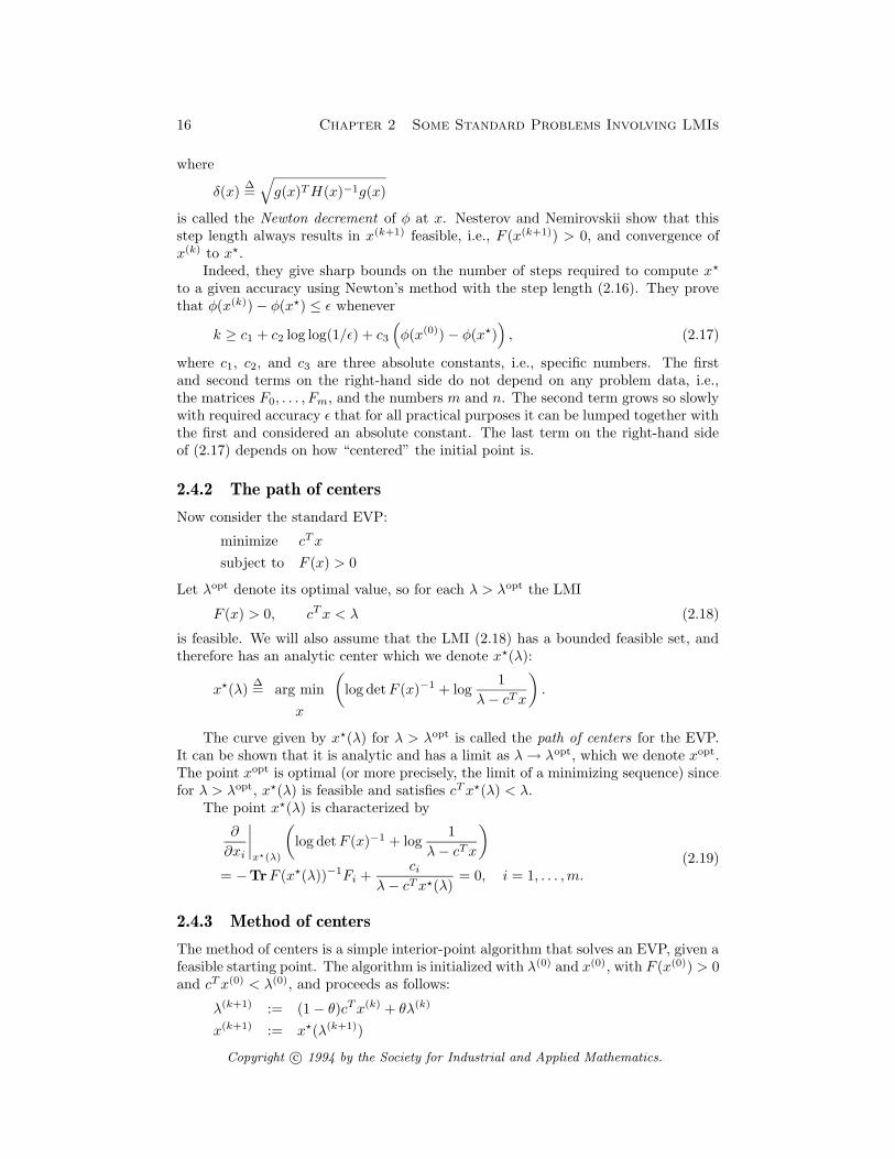
where
δ(x)∆=√
g(x)TH(x)−1g(x)
is called the Newton decrement of φ at x. Nesterov and Nemirovskii show that thisstep length always results in x(k+1) feasible, i.e., F (x(k+1)) > 0, and convergence ofx(k) to x?.
Indeed, they give sharp bounds on the number of steps required to compute x?
to a given accuracy using Newton’s method with the step length (2.16). They provethat φ(x(k))− φ(x?) ≤ ε whenever
k ≥ c1 + c2 log log(1/ε) + c3
(
φ(x(0))− φ(x?))
, (2.17)
where c1, c2, and c3 are three absolute constants, i.e., specific numbers. The firstand second terms on the right-hand side do not depend on any problem data, i.e.,the matrices F0, . . . , Fm, and the numbers m and n. The second term grows so slowlywith required accuracy ε that for all practical purposes it can be lumped together withthe first and considered an absolute constant. The last term on the right-hand sideof (2.17) depends on how “centered” the initial point is.
2.4.2 The path of centers
Now consider the standard EVP:
minimize cTx
subject to F (x) > 0
Let λopt denote its optimal value, so for each λ > λopt the LMI
F (x) > 0, cTx < λ (2.18)
is feasible. We will also assume that the LMI (2.18) has a bounded feasible set, andtherefore has an analytic center which we denote x?(λ):
x?(λ)∆= arg min
x
(
log detF (x)−1 + log1
λ− cTx
)
.
The curve given by x?(λ) for λ > λopt is called the path of centers for the EVP.It can be shown that it is analytic and has a limit as λ→ λopt, which we denote xopt.The point xopt is optimal (or more precisely, the limit of a minimizing sequence) sincefor λ > λopt, x?(λ) is feasible and satisfies cTx?(λ) < λ.
The point x?(λ) is characterized by
∂
∂xi
∣
∣
∣
∣
x?(λ)
(
log detF (x)−1 + log1
λ− cTx
)
= −TrF (x?(λ))−1Fi +ci
λ− cTx?(λ)= 0, i = 1, . . . ,m.
(2.19)
2.4.3 Method of centers
The method of centers is a simple interior-point algorithm that solves an EVP, given afeasible starting point. The algorithm is initialized with λ(0) and x(0), with F (x(0)) > 0and cTx(0) < λ(0), and proceeds as follows:
λ(k+1) := (1− θ)cTx(k) + θλ(k)
x(k+1) := x?(λ(k+1))
Copyright c© 1994 by the Society for Industrial and Applied Mathematics.
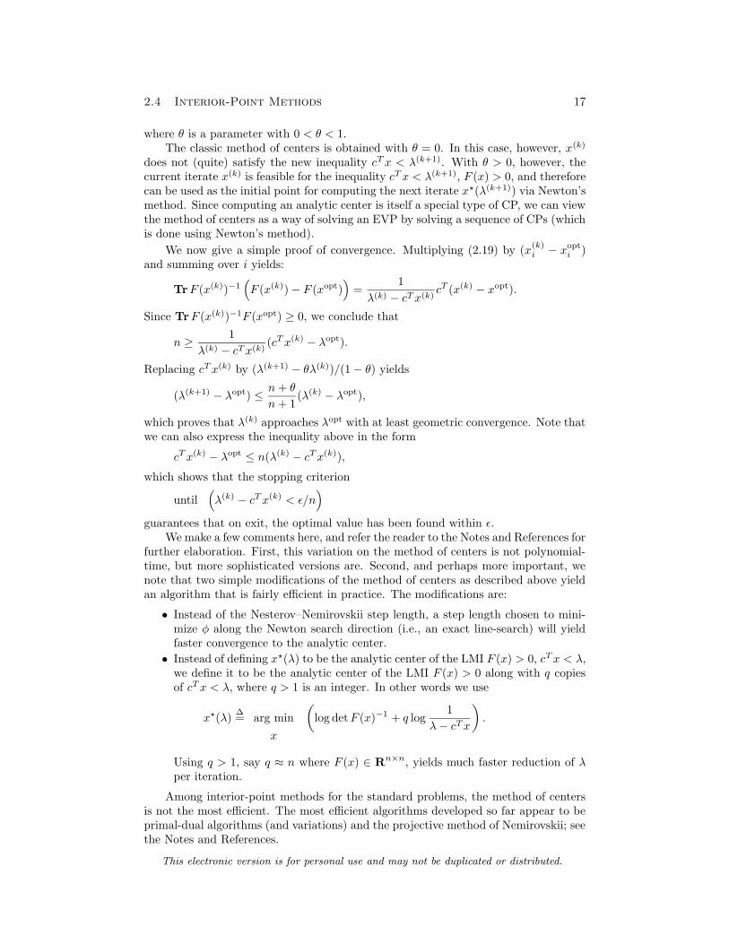
2.4 Interior-Point Methods 17
where θ is a parameter with 0 < θ < 1.The classic method of centers is obtained with θ = 0. In this case, however, x(k)
does not (quite) satisfy the new inequality cTx < λ(k+1). With θ > 0, however, thecurrent iterate x(k) is feasible for the inequality cTx < λ(k+1), F (x) > 0, and thereforecan be used as the initial point for computing the next iterate x?(λ(k+1)) via Newton’smethod. Since computing an analytic center is itself a special type of CP, we can viewthe method of centers as a way of solving an EVP by solving a sequence of CPs (whichis done using Newton’s method).
We now give a simple proof of convergence. Multiplying (2.19) by (x(k)i − xopti )
and summing over i yields:
TrF (x(k))−1(
F (x(k))− F (xopt))
=1
λ(k) − cTx(k)cT (x(k) − xopt).
Since TrF (x(k))−1F (xopt) ≥ 0, we conclude that
n ≥ 1
λ(k) − cTx(k)(cTx(k) − λopt).
Replacing cTx(k) by (λ(k+1) − θλ(k))/(1− θ) yields
(λ(k+1) − λopt) ≤ n+ θ
n+ 1(λ(k) − λopt),
which proves that λ(k) approaches λopt with at least geometric convergence. Note thatwe can also express the inequality above in the form
cTx(k) − λopt ≤ n(λ(k) − cTx(k)),
which shows that the stopping criterion
until(
λ(k) − cTx(k) < ε/n)
guarantees that on exit, the optimal value has been found within ε.We make a few comments here, and refer the reader to the Notes and References for
further elaboration. First, this variation on the method of centers is not polynomial-time, but more sophisticated versions are. Second, and perhaps more important, wenote that two simple modifications of the method of centers as described above yieldan algorithm that is fairly efficient in practice. The modifications are:
• Instead of the Nesterov–Nemirovskii step length, a step length chosen to mini-mize φ along the Newton search direction (i.e., an exact line-search) will yieldfaster convergence to the analytic center.
• Instead of defining x?(λ) to be the analytic center of the LMI F (x) > 0, cTx < λ,we define it to be the analytic center of the LMI F (x) > 0 along with q copiesof cTx < λ, where q > 1 is an integer. In other words we use
x?(λ)∆= arg min
x
(
log detF (x)−1 + q log1
λ− cTx
)
.
Using q > 1, say q ≈ n where F (x) ∈ Rn×n, yields much faster reduction of λper iteration.
Among interior-point methods for the standard problems, the method of centersis not the most efficient. The most efficient algorithms developed so far appear to beprimal-dual algorithms (and variations) and the projective method of Nemirovskii; seethe Notes and References.
This electronic version is for personal use and may not be duplicated or distributed.
18 Chapter 2 Some Standard Problems Involving LMIs
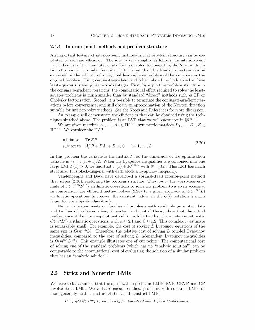
2.4.4 Interior-point methods and problem structure
An important feature of interior-point methods is that problem structure can be ex-ploited to increase efficiency. The idea is very roughly as follows. In interior-pointmethods most of the computational effort is devoted to computing the Newton direc-tion of a barrier or similar function. It turns out that this Newton direction can beexpressed as the solution of a weighted least-squares problem of the same size as theoriginal problem. Using conjugate-gradient and other related methods to solve theseleast-squares systems gives two advantages. First, by exploiting problem structure inthe conjugate-gradient iterations, the computational effort required to solve the least-squares problems is much smaller than by standard “direct” methods such as QR orCholesky factorization. Second, it is possible to terminate the conjugate-gradient iter-ations before convergence, and still obtain an approximation of the Newton directionsuitable for interior-point methods. See the Notes and References for more discussion.
An example will demonstrate the efficiencies that can be obtained using the tech-niques sketched above. The problem is an EVP that we will encounter in §6.2.1.
We are given matrices A1, . . . , AL ∈ Rn×n, symmetric matrices D1, . . . , DL, E ∈Rn×n. We consider the EVP
minimize TrEP
subject to ATi P + PAi +Di < 0, i = 1, . . . , L
(2.20)
In this problem the variable is the matrix P , so the dimension of the optimizationvariable is m = n(n + 1)/2. When the Lyapunov inequalities are combined into onelarge LMI F (x) > 0, we find that F (x) ∈ RN×N with N = Ln. This LMI has muchstructure: It is block-diagonal with each block a Lyapunov inequality.
Vandenberghe and Boyd have developed a (primal-dual) interior-point methodthat solves (2.20), exploiting the problem structure. They prove the worst-case esti-mate of O(m2.75L1.5) arithmetic operations to solve the problem to a given accuracy.In comparison, the ellipsoid method solves (2.20) to a given accuracy in O(m3.5L)arithmetic operations (moreover, the constant hidden in the O(·) notation is muchlarger for the ellipsoid algorithm).
Numerical experiments on families of problems with randomly generated dataand families of problems arising in system and control theory show that the actualperformance of the interior-point method is much better than the worst-case estimate:O(mαLβ) arithmetic operations, with α ≈ 2.1 and β ≈ 1.2. This complexity estimateis remarkably small. For example, the cost of solving L Lyapunov equations of thesame size is O(m1.5L). Therefore, the relative cost of solving L coupled Lyapunovinequalities, compared to the cost of solving L independent Lyapunov inequalitiesis O(m0.6L0.2). This example illustrates one of our points: The computational costof solving one of the standard problems (which has no “analytic solution”) can becomparable to the computational cost of evaluating the solution of a similar problemthat has an “analytic solution”.
2.5 Strict and Nonstrict LMIs
We have so far assumed that the optimization problems LMIP, EVP, GEVP, and CPinvolve strict LMIs. We will also encounter these problems with nonstrict LMIs, ormore generally, with a mixture of strict and nonstrict LMIs.
Copyright c© 1994 by the Society for Industrial and Applied Mathematics.
2.5 Strict and Nonstrict LMIs 19
As an example consider the nonstrict version of the EVP (2.9), i.e.
minimize cTx
subject to F (x) ≥ 0
Intuition suggests that we could simply solve the strict EVP (by, say, an interior-pointmethod) to obtain the solution of the nonstrict EVP. This is correct in most but notall cases.
If the strict LMI F (x) > 0 is feasible, then we have
x ∈ Rm | F (x) ≥ 0 = x ∈ Rm | F (x) > 0, (2.21)
i.e., the feasible set of the nonstrict LMI is the closure of the feasible set of the strictLMI. It follows that
inf
cTx | F (x) ≥ 0
= inf
cTx | F (x) > 0
. (2.22)
So in this case, we can solve the strict EVP to obtain a solution of the nonstrict EVP.This is true for the problems GEVP and CP as well.
We will say that the LMI F (x) ≥ 0 is strictly feasible if its strict version is feasible,i.e., if there is some x0 ∈ Rm such that F (x0) > 0. We have just seen that when anLMI is strictly feasible, we can replace nonstrict inequality with strict inequality in theproblems EVP, GEVP, and CP in order to solve them. In the language of optimizationtheory, the requirement of strict feasibility is a (very strong) constraint qualification.
When an LMI is feasible but not strictly feasible, (2.21) need not hold, and theEVPs with the strict and nonstrict LMIs can be very different. As a simple example,consider F (x) = diag(x,−x) with x ∈ R. The right-hand side of (2.22) is +∞ sincethe strict LMI F (x) > 0 is infeasible. The left-hand side, however, is always 0, sincethe LMI F (x) ≥ 0 has the single feasible point x = 0. This example shows one of thetwo pathologies that can occur: The nonstrict inequality contains an implicit equalityconstraint (in contrast with an explicit equality constraint as in §2.1.2).
The other pathology is demonstrated by the example F (x) = diag(x, 0) withx ∈ R and c = −1. Once again, the strict LMI is infeasible so the right-hand sideof (2.22) is +∞. The feasible set for the nonstrict LMI is the interval [0, ∞) so theright-hand side is −∞. The problem here is that F (x) is always singular. Of course,the nonstrict LMI F (x) ≥ 0 is equivalent (in the sense of defining equal feasible sets) tothe “reduced” LMI F (x) = x ≥ 0. Note that this reduced LMI satisfies the constraintqualification, i.e., is strictly feasible.
2.5.1 Reduction to a strictly feasible LMI
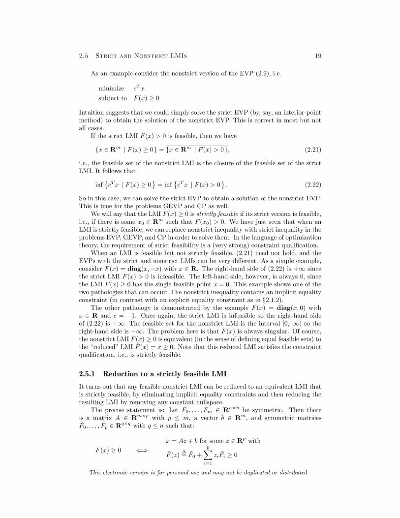
It turns out that any feasible nonstrict LMI can be reduced to an equivalent LMI thatis strictly feasible, by eliminating implicit equality constraints and then reducing theresulting LMI by removing any constant nullspace.
The precise statement is: Let F0, . . . , Fm ∈ Rn×n be symmetric. Then thereis a matrix A ∈ Rm×p with p ≤ m, a vector b ∈ Rm, and symmetric matricesF0, . . . , Fp ∈ Rq×q with q ≤ n such that:
F (x) ≥ 0 ⇐⇒x = Az + b for some z ∈ Rp with
F (z)∆= F0 +
p∑
i=1
ziFi ≥ 0
This electronic version is for personal use and may not be duplicated or distributed.
20 Chapter 2 Some Standard Problems Involving LMIs
where the LMI F (z) ≥ 0 is either infeasible or strictly feasible. See the Notes andReferences for a proof.
The matrix A and vector b describe the implicit equality constraints for the LMIF (x) ≥ 0. Similarly, the LMI F (z) ≥ 0 can be interpreted as the original LMI withits constant nullspace removed (see the Notes and References). In most of the prob-lems encountered in this book, there are no implicit equality constraints or nontrivialcommon nullspace for F , so we can just take A = I, b = 0, and F = F .
Using this reduction we can, at least in principle, always deal with strictly feasibleLMIs. For example we have
inf
cTx∣
∣ F (x) ≥ 0
= inf
cT (Az + b)∣
∣
∣F (z) ≥ 0
= inf
cT (Az + b)∣
∣
∣F (z) > 0
since the LMI F (z) ≥ 0 is either infeasible or strictly feasible.
2.5.2 Example: Lyapunov inequality
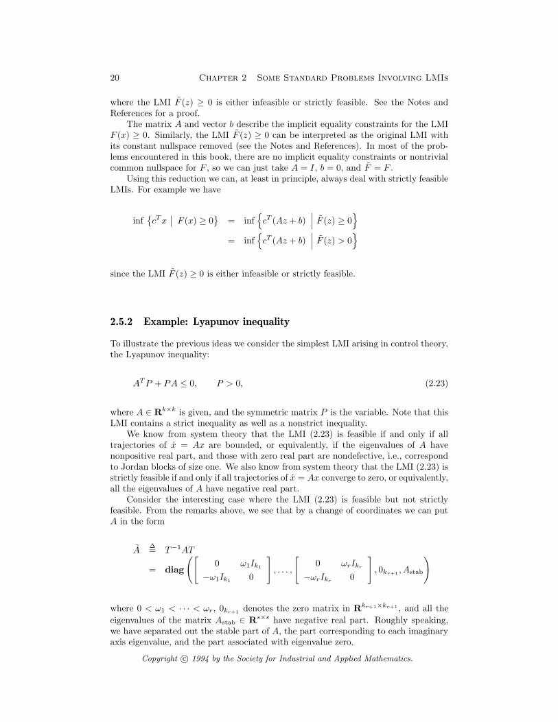
To illustrate the previous ideas we consider the simplest LMI arising in control theory,the Lyapunov inequality:
ATP + PA ≤ 0, P > 0, (2.23)
where A ∈ Rk×k is given, and the symmetric matrix P is the variable. Note that thisLMI contains a strict inequality as well as a nonstrict inequality.
We know from system theory that the LMI (2.23) is feasible if and only if alltrajectories of x = Ax are bounded, or equivalently, if the eigenvalues of A havenonpositive real part, and those with zero real part are nondefective, i.e., correspondto Jordan blocks of size one. We also know from system theory that the LMI (2.23) isstrictly feasible if and only if all trajectories of x = Ax converge to zero, or equivalently,all the eigenvalues of A have negative real part.
Consider the interesting case where the LMI (2.23) is feasible but not strictlyfeasible. From the remarks above, we see that by a change of coordinates we can putA in the form
A∆= T−1AT
= diag
([
0 ω1Ik1
−ω1Ik10
]
, . . . ,
[
0 ωrIkr
−ωrIkr0
]
, 0kr+1, Astab
)
where 0 < ω1 < · · · < ωr, 0kr+1denotes the zero matrix in Rkr+1×kr+1 , and all the
eigenvalues of the matrix Astab ∈ Rs×s have negative real part. Roughly speaking,we have separated out the stable part of A, the part corresponding to each imaginaryaxis eigenvalue, and the part associated with eigenvalue zero.
Copyright c© 1994 by the Society for Industrial and Applied Mathematics.
2.5 Strict and Nonstrict LMIs 21
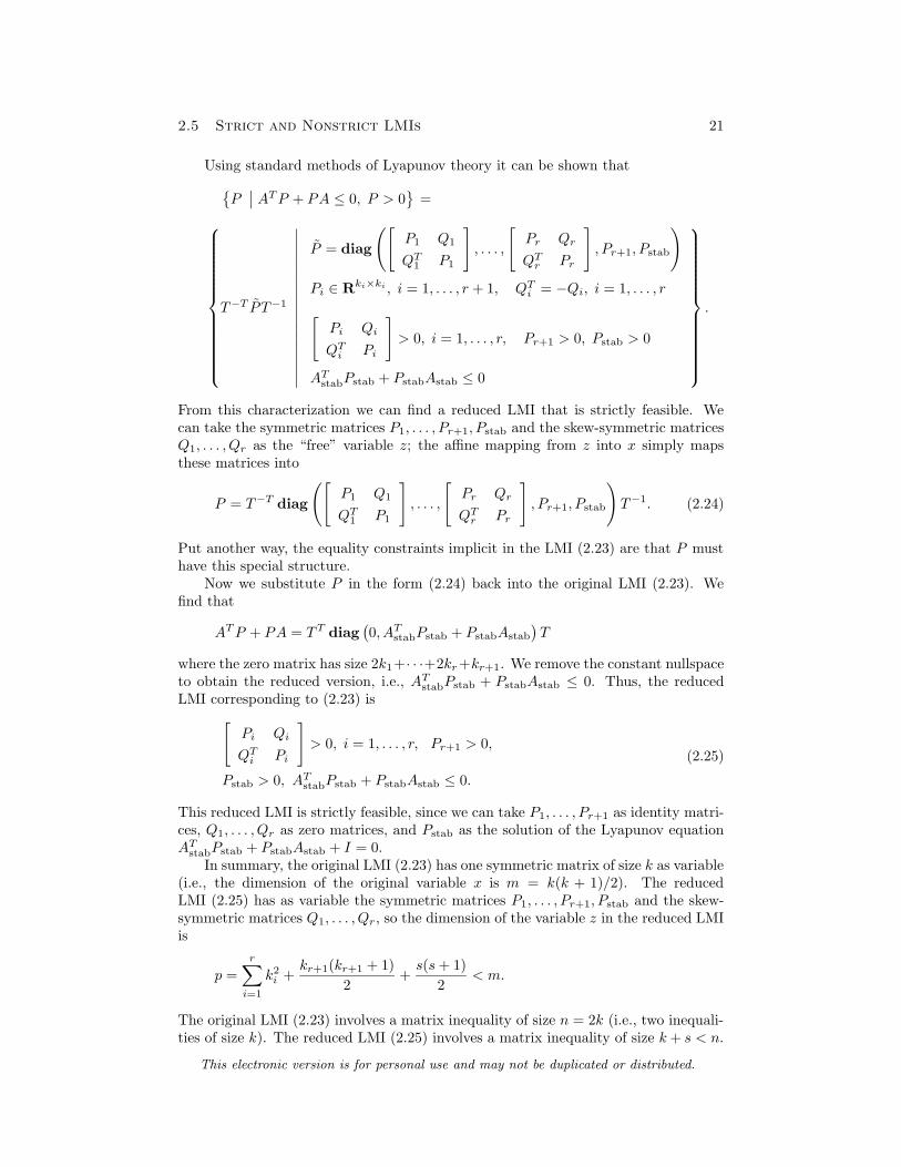
Using standard methods of Lyapunov theory it can be shown that
P∣
∣ ATP + PA ≤ 0, P > 0
=
T−T P T−1
∣
∣
∣
∣
∣
∣
∣
∣
∣
∣
∣
∣
∣
∣
∣
∣
∣
∣
P = diag
([
P1 Q1
QT1 P1
]
, . . . ,
[
Pr Qr
QTr Pr
]
, Pr+1, Pstab
)
Pi ∈ Rki×ki , i = 1, . . . , r + 1, QTi = −Qi, i = 1, . . . , r
[
Pi Qi
QTi Pi
]
> 0, i = 1, . . . , r, Pr+1 > 0, Pstab > 0
ATstabPstab + PstabAstab ≤ 0
.
From this characterization we can find a reduced LMI that is strictly feasible. Wecan take the symmetric matrices P1, . . . , Pr+1, Pstab and the skew-symmetric matricesQ1, . . . , Qr as the “free” variable z; the affine mapping from z into x simply mapsthese matrices into
P = T−T diag
([
P1 Q1
QT1 P1
]
, . . . ,
[
Pr Qr
QTr Pr
]
, Pr+1, Pstab
)
T−1. (2.24)
Put another way, the equality constraints implicit in the LMI (2.23) are that P musthave this special structure.
Now we substitute P in the form (2.24) back into the original LMI (2.23). Wefind that
ATP + PA = T T diag(
0, ATstabPstab + PstabAstab
)
T
where the zero matrix has size 2k1+· · ·+2kr+kr+1. We remove the constant nullspaceto obtain the reduced version, i.e., AT
stabPstab + PstabAstab ≤ 0. Thus, the reducedLMI corresponding to (2.23) is
[
Pi Qi
QTi Pi
]
> 0, i = 1, . . . , r, Pr+1 > 0,
Pstab > 0, ATstabPstab + PstabAstab ≤ 0.
(2.25)
This reduced LMI is strictly feasible, since we can take P1, . . . , Pr+1 as identity matri-ces, Q1, . . . , Qr as zero matrices, and Pstab as the solution of the Lyapunov equationATstabPstab + PstabAstab + I = 0.
In summary, the original LMI (2.23) has one symmetric matrix of size k as variable(i.e., the dimension of the original variable x is m = k(k + 1)/2). The reducedLMI (2.25) has as variable the symmetric matrices P1, . . . , Pr+1, Pstab and the skew-symmetric matrices Q1, . . . , Qr, so the dimension of the variable z in the reduced LMIis
p =
r∑
i=1
k2i +kr+1(kr+1 + 1)
2+s(s+ 1)
2< m.
The original LMI (2.23) involves a matrix inequality of size n = 2k (i.e., two inequali-ties of size k). The reduced LMI (2.25) involves a matrix inequality of size k+ s < n.
This electronic version is for personal use and may not be duplicated or distributed.
22 Chapter 2 Some Standard Problems Involving LMIs
2.6 Miscellaneous Results on Matrix Inequalities
2.6.1 Elimination of semidefinite terms
In the LMIP
find x such that F (x) > 0, (2.26)
we can eliminate any variables for which the corresponding coefficient in F is semidef-inite. Suppose for example that Fm ≥ 0 and has rank r < n. Roughly speaking, bytaking xm extremely large, we can ensure that F is positive-definite on the range ofFm, so the LMIP reduces to making F positive-definite on the nullspace of Fm.
More precisely, let Fm = UUT with U full-rank, and let U be an orthogonalcomplement of U , e.g., UT U = 0 and [U U ] is of maximum rank (which in this casejust means that [U U ] is nonsingular). Of course, we have
F (x) > 0 ⇐⇒[
U U]T
F (x)[
U U]
> 0.
Since
[
U U]T
F (x)[
U U]
=
[
UT F (x)U UT F (x)U
UT F (x)U UT F (x)U + xm(UTU)2
]
,
where x = [x1 · · ·xm−1]T and F (x)∆= F0 + x1F1 + · · · + xm−1Fm−1, we see that
F (x) > 0 if and only if UT F U(x) > 0, and xm is large enough that
UT F (x)U + xm(UTU)2 > UT F (x)U(
UT F (x)U)−1
UT F (x)U.
Therefore, the LMIP (2.26) is equivalent to
find x1, . . . , xm−1 such that UT F (x1, . . . , xm−1)U > 0.
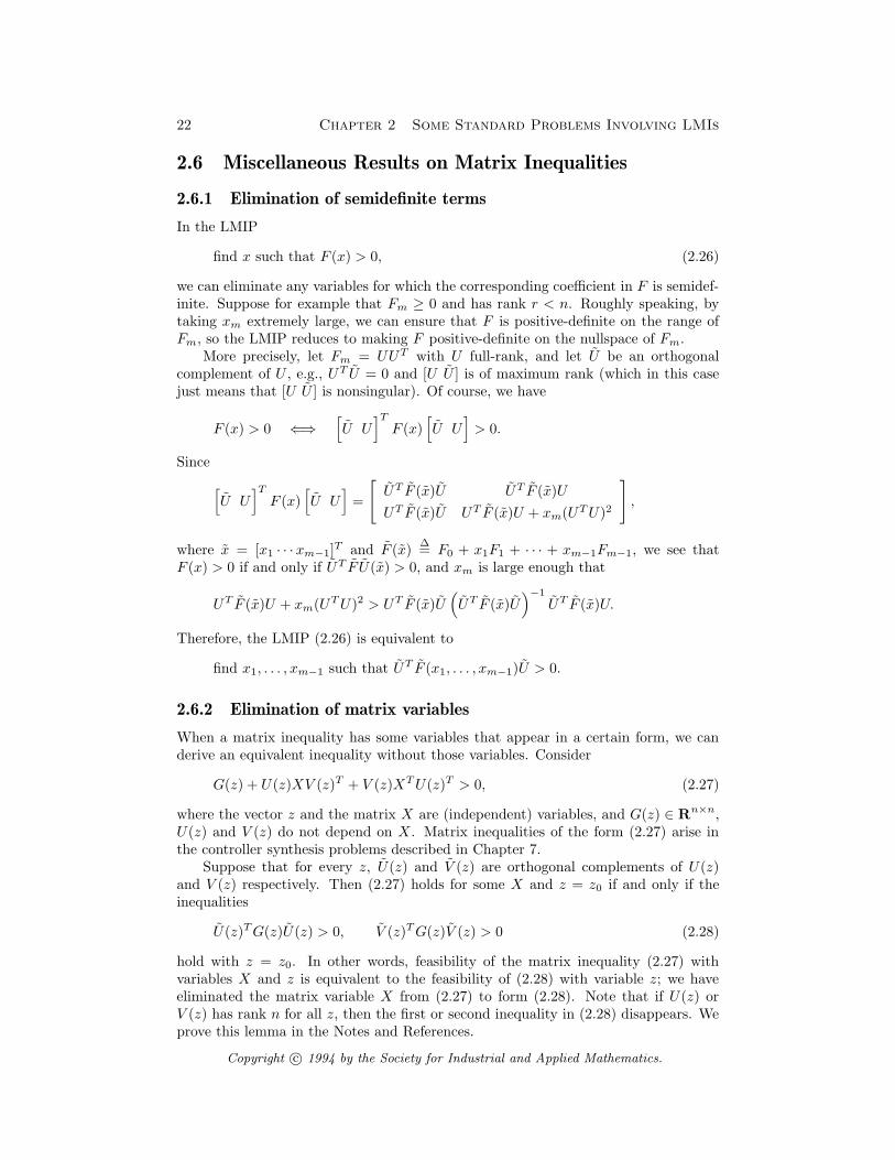
2.6.2 Elimination of matrix variables
When a matrix inequality has some variables that appear in a certain form, we canderive an equivalent inequality without those variables. Consider
G(z) + U(z)XV (z)T + V (z)XTU(z)T > 0, (2.27)
where the vector z and the matrix X are (independent) variables, and G(z) ∈ Rn×n,U(z) and V (z) do not depend on X. Matrix inequalities of the form (2.27) arise inthe controller synthesis problems described in Chapter 7.
Suppose that for every z, U(z) and V (z) are orthogonal complements of U(z)and V (z) respectively. Then (2.27) holds for some X and z = z0 if and only if theinequalities
U(z)TG(z)U(z) > 0, V (z)TG(z)V (z) > 0 (2.28)
hold with z = z0. In other words, feasibility of the matrix inequality (2.27) withvariables X and z is equivalent to the feasibility of (2.28) with variable z; we haveeliminated the matrix variable X from (2.27) to form (2.28). Note that if U(z) orV (z) has rank n for all z, then the first or second inequality in (2.28) disappears. Weprove this lemma in the Notes and References.
Copyright c© 1994 by the Society for Industrial and Applied Mathematics.
2.6 Miscellaneous Results on Matrix Inequalities 23
We can express (2.28) in another form using Finsler’s lemma (see the Notes andReferences):
G(z)− σU(z)U(z)T > 0, G(z)− σV (z)V (z)T > 0
for some σ ∈ R.As an example, we will encounter in §7.2.1 the LMIP with LMI
Q > 0, AQ+QAT +BY + Y TBT < 0, (2.29)
where Q and Y are the variables. This LMIP is equivalent to the LMIP with LMI
Q > 0, AQ+QAT < σBBT ,
where the variables are Q and σ ∈ R. It is also equivalent to the LMIP
Q > 0, BT(
AQ+QAT)
B < 0,
with variable Q, where B is any matrix of maximum rank such that BTB = 0. Thuswe have eliminated the variable Y from (2.29) and reduced the size of the matrices inthe LMI.
2.6.3 The S-procedureWe will often encounter the constraint that some quadratic function (or quadraticform) be negative whenever some other quadratic functions (or quadratic forms) areall negative. In some cases, this constraint can be expressed as an LMI in the datadefining the quadratic functions or forms; in other cases, we can form an LMI that isa conservative but often useful approximation of the constraint.
The S-procedure for quadratic functions and nonstrict inequalitiesLet F0, . . . , Fp be quadratic functions of the variable ζ ∈ Rn:
Fi(ζ)∆= ζTTiζ + 2uTi ζ + vi, i = 0, . . . , p,
where Ti = TTi . We consider the following condition on F0, . . . , Fp:
F0(ζ) ≥ 0 for all ζ such that Fi(ζ) ≥ 0, i = 1, . . . , p. (2.30)
Obviously if
there exist τ1 ≥ 0, . . . , τp ≥ 0 such that
for all ζ, F0(ζ)−p∑
i=1
τiFi(ζ) ≥ 0,(2.31)
then (2.30) holds. It is a nontrivial fact that when p = 1, the converse holds, providedthat there is some ζ0 such that F1(ζ0) > 0.
Remark: If the functions Fi are affine, then (2.31) and (2.30) are equivalent;this is the Farkas lemma.
Note that (2.31) can be written as[
T0 u0
uT0 v0
]
−p∑
i=1
τi
[
Ti ui
uTi vi
]
≥ 0.
This electronic version is for personal use and may not be duplicated or distributed.
24 Chapter 2 Some Standard Problems Involving LMIs
The S-procedure for quadratic forms and strict inequalities
We will use another variation of the S-procedure, which involves quadratic forms andstrict inequalities. Let T0, . . . , Tp ∈ Rn×n be symmetric matrices. We consider thefollowing condition on T0, . . . , Tp:
ζTT0ζ > 0 for all ζ 6= 0 such that ζTTiζ ≥ 0, i = 1, . . . , p. (2.32)
It is obvious that if
there exists τ1 ≥ 0, . . . , τp ≥ 0 such that T0 −p∑
i=1
τiTi > 0, (2.33)
then (2.32) holds. It is a nontrivial fact that when p = 1, the converse holds, providedthat there is some ζ0 such that ζT0 T1ζ0 > 0. Note that (2.33) is an LMI in the variablesT0 and τ1, . . . , τp.
Remark: The first version of the S-procedure deals with nonstrict inequalitiesand quadratic functions that may include constant and linear terms. The secondversion deals with strict inequalities and quadratic forms only, i.e., quadraticfunctions without constant or linear terms.
Remark: Suppose that T0, u0 and v0 depend affinely on some parameter ν. Thenthe condition (2.30) is convex in ν. This does not, however, mean that the problemof checking whether there exists ν such that (2.30) holds has low complexity. Onthe other hand, checking whether (2.31) holds for some ν is an LMIP in thevariables ν and τ1, . . . , τp. Therefore, this problem has low complexity. See theNotes and References for further discussion.
S-procedure exampleIn Chapter 5 we will encounter the following constraint on the variable P :
for all ξ 6= 0 and π satisfying πTπ ≤ ξTCTCξ,[
ξ
π
]T [
ATP + PA PB
BTP 0
][
ξ
π
]
< 0.(2.34)
Applying the second version of the S-procedure, (2.34) is equivalent to the existenceof τ ≥ 0 such that
ATP + PA+ τCTC PB
BTP −τI
< 0.
Thus the problem of finding P > 0 such that (2.34) holds can be expressed as anLMIP (in P and the scalar variable τ).
2.7 Some LMI Problems with Analytic Solutions
There are analytic solutions to several LMI problems of special form, often with im-portant system and control theoretic interpretations. We briefly describe some of theseresults in this section. At the same time we introduce and define several importantterms from system and control theory.
Copyright c© 1994 by the Society for Industrial and Applied Mathematics.
2.7 Some LMI Problems with Analytic Solutions 25
2.7.1 Lyapunov’s inequality
We have already mentioned the LMIP associated with Lyapunov’s inequality, i.e.
P > 0, ATP + PA < 0
where P is variable and A ∈ Rn×n is given. Lyapunov showed that this LMI is feasibleif and only the matrix A is stable, i.e., all trajectories of x = Ax converge to zero ast→∞, or equivalently, all eigenvalues of A must have negative real part. To solve thisLMIP, we pick any Q > 0 and solve the Lyapunov equation ATP + PA = −Q, whichis nothing but a set of n(n+ 1)/2 linear equations for the n(n+ 1)/2 scalar variablesin P . This set of linear equations will be solvable and result in P > 0 if and only ifthe LMI is feasible. In fact this procedure not only finds a solution when the LMI isfeasible; it parametrizes all solutions as Q varies over the positive-definite cone.
2.7.2 The positive-real lemma
Another important example is given by the positive-real (PR) lemma, which yieldsa “frequency-domain” interpretation for a certain LMIP, and under some additionalassumptions, a numerical solution procedure via Riccati equations as well. We give asimplified discussion here, and refer the reader to the References for more completestatements.
The LMI considered is:
P > 0,
[
ATP + PA PB − CT
BTP − C −DT −D
]
≤ 0, (2.35)
where A ∈ Rn×n, B ∈ Rn×p, C ∈ Rp×n, and D ∈ Rp×p are given, and the matrixP = PT ∈ Rn×n is the variable. (We will encounter a variation on this LMI in §6.3.3.)Note that if D + DT > 0, the LMI (2.35) is equivalent to the quadratic matrixinequality
ATP + PA+ (PB − CT )(D +DT )−1(PB − CT )T ≤ 0. (2.36)
We assume for simplicity that A is stable and the system (A,B,C) is minimal.The link with system and control theory is given by the following result. The
LMI (2.35) is feasible if and only if the linear system
x = Ax+Bu, y = Cx+Du (2.37)
is passive, i.e.,
∫ T
0
u(t)T y(t) dt ≥ 0
for all solutions of (2.37) with x(0) = 0.Passivity can also be expressed in terms of the transfer matrix of the linear sys-
tem (2.37), defined as
H(s)∆= C(sI −A)−1B +D
for s ∈ C. Passivity is equivalent to the transfer matrix H being positive-real, whichmeans that
H(s) +H(s)∗ ≥ 0 for all Re s > 0.
This electronic version is for personal use and may not be duplicated or distributed.
26 Chapter 2 Some Standard Problems Involving LMIs
When p = 1 this condition can be checked by various graphical means, e.g., plottingthe curve given by the real and imaginary parts of H(iω) for ω ∈ R (called the Nyquistplot of the linear system). Thus we have a graphical, frequency-domain condition forfeasibility of the LMI (2.35). This approach was used in much of the work in the 1960sand 1970s described in §1.2.
With a few further technical assumptions, including D+DT > 0, the LMI (2.35)can be solved by a method based on Riccati equations and Hamiltonian matrices.With these assumptions the LMI (2.35) is feasible if and only if there exists a realmatrix P = P T satisfying the ARE
ATP + PA+ (PB − CT )(D +DT )−1(PB − CT )T = 0, (2.38)
which is just the quadratic matrix inequality (2.36) with equality substituted for in-equality. Note that P > 0.
To solve the ARE (2.38) we first form the associated Hamiltonian matrix
M =
[
A−B(D +DT )−1C B(D +DT )−1BT
−CT (D +DT )−1C −AT + CT (D +DT )−1BT
]
.
Then the system (2.37) is passive, or equivalently, the LMI (2.35) is feasible, if andonly if M has no pure imaginary eigenvalues. This fact can be used to form a Routh–Hurwitz (Sturm) type test for passivity as a set of polynomial inequalities in the dataA, B, C, and D.
When M has no pure imaginary eigenvalues we can construct a solution Pare asfollows. Pick V ∈ R2n×n so that its range is a basis for the stable eigenspace ofM , e.g., V = [v1 · · · vn] where v1, . . . , vn are a set of independent eigenvectors of Massociated with its n eigenvalues with negative real part. Partition V as
V =
[
V1
V2
]
,
where V1 and V2 are square; then set Pare = V2V−11 . The solution Pare thus obtained
is the minimal element among the set of solutions of (2.38): if P = P T satisfies (2.38),then P ≥ Pare. Much more discussion of this method, including the precise technicalconditions, can be found in the References.
2.7.3 The bounded-real lemma
The same results appear in another important form, the bounded-real lemma. Herewe consider the LMI
P > 0,
[
ATP + PA+ CTC PB + CTD
BTP +DTC DTD − I
]
≤ 0. (2.39)
where A ∈ Rn×n, B ∈ Rn×p, C ∈ Rp×n, and D ∈ Rp×p are given, and the matrixP = PT ∈ Rn×n is the variable. For simplicity we assume that A is stable and(A,B,C) is minimal.
This LMI is feasible if and only the linear system (2.37) is nonexpansive, i.e.,
∫ T
0
y(t)T y(t) dt ≤∫ T
0
u(t)Tu(t) dt
Copyright c© 1994 by the Society for Industrial and Applied Mathematics.
Notes and References 27
for all solutions of (2.37) with x(0) = 0, This condition can also be expressed interms of the transfer matrix H. Nonexpansivity is equivalent to the transfer matrixH satisfying the bounded-real condition, i.e.,
H(s)∗H(s) ≤ I for all Re s > 0.
This is sometimes expressed as ‖H‖∞ ≤ 1 where
‖H‖∞ ∆= sup ‖H(s)‖ | Re s > 0
is called the H∞ norm of the transfer matrix H.This condition is easily checked graphically, e.g., by plotting ‖H(iω)‖ versus ω ∈ R
(called a singular value plot for p > 1 and a Bode magnitude plot for p = 1).Once again we can relate the LMI (2.39) to an ARE. With some appropriate tech-
nical conditions (see the Notes and References) including DTD < I, the LMI (2.39)is feasible if and only the ARE
ATP + PA+ CTC + (PB + CTD)(I −DTD)−1(PB + CTD)T = 0 (2.40)
has a real solution P = P T . Once again this is the quadratic matrix inequalityassociated with the LMI (2.39), with equality instead of the inequality.
We can solve this equation by forming the Hamiltonian matrix
M =
[
A+B(I −DTD)−1DTC B(I −DTD)−1BT
−CT (I −DDT )−1C −AT − CTD(I −DTD)−1BT
]
.
Then the system (2.37) is nonexpansive, or equivalently, the LMI (2.39) is feasible,if and only if M has no imaginary eigenvalues. In this case we can find the minimalsolution to (2.40) as described in §2.7.2.
2.7.4 Others
Several other LMI problems have analytic solutions, e.g., the ones that arise in thesynthesis of state-feedback for linear systems, or estimator gains for observers. As asimple example consider the LMI
P > 0, AP + PAT < BBT
where A ∈ Rn×n and B ∈ Rn×p are given and P is the variable. This LMI is feasibleif and only if the pair (A,B) is stabilizable, i.e., there exists a matrix K ∈ Rp×n suchthat A+BK is stable. There are simple methods for determining whether this is thecase, and when it is, of constructing an appropriate P . We will describe this and otherresults in Chapter 7.
Several standard results from linear algebra can also be interpreted as analyticsolutions to certain LMI problems of special form. For example, it is well-knownthat among all symmetric positive-definite matrices with given diagonal elements,the diagonal matrix has maximum determinant. This gives an analytic solution to aspecial (and fairly trivial) CP (see §3.5).
Notes and References
LMIs
The term “Linear Matrix Inequality” was coined by J. C. Willems and is widely used now.As we mentioned in §1.2, the term was used in several papers from the 1970s to refer to the
This electronic version is for personal use and may not be duplicated or distributed.

28 Chapter 2 Some Standard Problems Involving LMIs
specific LMI (1.3). The term is also consistent with the title of an early paper by Bellmanand Ky Fan: On Systems of Linear Inequalities in Hermitian Matrix Variables [BF63] (seebelow).
A more accurate term might be “Affine Matrix Inequality”, since the matrix is an affineand not linear function of the variable. We think of the term “Linear Matrix Inequality” asanalogous to the term “Linear Inequalities” used to describe aTi x ≤ bi, i = 1, . . . , p.
When m = 1, an LMI is nothing but a matrix pencil. The theory of matrix pencils is very oldand quite complete, and there is an extensive literature (see, e.g., Golub and Van Loan [GL89]and the references therein). For the case of m = 1 all of our standard problems are readilysolved, e.g., by simultaneous diagonalization of F0 and F1 by an appropriate congruence.The case m = 1 does not arise on its own in any interesting problem from system or controltheory, but it does arise in the “line-search (sub)problem”, i.e., when we restrict one of ourstandard problems to a specific line. In this context the variable represents the “step length”to be taken in an iteration of an algorithm, and it useful to know that such problems can besolved extremely efficiently.
Schur complements for nonstrict inequalities
The Schur complement result of section §2.1 can be generalized to nonstrict inequalities asfollows. Suppose Q and R are symmetric. The condition
[
Q S
ST R
]
≥ 0 (2.41)
is equivalent to
R ≥ 0, Q− SR†ST ≥ 0, S(I −RR†) = 0,
where R† denotes the Moore–Penrose inverse of R.
To see this, let U be an orthogonal matrix that diagonalizes R, so that
UTRU =
[
Σ 0
0 0
]
,
where Σ > 0 and diagonal. Inequality (2.41) holds if and only if
[
I 0
0 UT
][
Q S
ST R
][
I 0
0 U
]
=
Q S1 S2
ST1 Σ 0
ST2 0 0
≥ 0,
where [S1 S2] = SU , with appropriate partitioning. We must then have S2 = 0, which holdsif and only if S(I −RR†) = 0, and
[
Q S1
ST1 Σ
]
≥ 0,
which holds if and only if Q− SR†ST ≥ 0.
Formulating convex problems in terms of LMIs
The idea that LMIs can be used to represent a wide variety of convex constraints can befound in Nesterov and Nemirovskii’s report [NN90b] (which is really a preliminary version
Copyright c© 1994 by the Society for Industrial and Applied Mathematics.
Notes and References 29
of their book [NN94]) and software manual [NN90a]. They formalize the idea of a “positive-definite representable” function; see §5.3, §5.4, and §6.4 of their book [NN94]. The ideais also discussed in the article [Ali92b] and thesis [Ali91] of Alizadeh. In [BE93], Boydand El Ghaoui give a list of quasiconvex functions that can be represented as generalizedeigenvalues of matrices that depend affinely on the variable.
Infeasibility criterion for LMIs
The LMI F (x) > 0 is infeasible means the affine set F (x) | x ∈ Rm does not intersect thepositive-definite cone. From convex analysis, this is equivalent to the existence of a linearfunctional ψ that is positive on the positive-definite cone and nonpositive on the affine setof matrices. The linear functionals that are positive on the positive-definite cone are of theform ψ(F ) = TrGF , where G ≥ 0 and G 6= 0. From the fact that ψ is nonpositive on theaffine set F (x)|x ∈ Rm, we can conclude that TrGFi = 0, i = 1, . . . ,m and TrGF0 ≤ 0.These are precisely the conditions for infeasibility of an LMI that we mentioned in §2.2.1.For the special case of multiple Lyapunov inequalities, these conditions are given Bellmanand Ky Fan [BF63] and Kamenetskii and Pyatnitskii [KP87a, KP87b].
It is straightforward to derive optimality criteria for the other problems, using convex anal-ysis. Some general references for convex analysis are the books [Roc70, Roc82] and surveyarticle [Roc93] by Rockafellar. The recent text [HUL93] gives a good overview of convexanalysis; LMIs are used as examples in several places.
Complexity of convex optimization
The important role of convexity in optimization is fairly widely known, but perhaps notwell enough appreciated, at least outside the former Soviet Union. In a standard (Western)treatment of optimization, our standard problems LMIP, EVP, GEVP, and CP would beconsidered very difficult since they are nondifferentiable and nonlinear. Their convexityproperties, however, make them tractable, both in theory and in practice.
In [Roc93, p194], Rockafellar makes the important point:
One distinguishing idea which dominates many issues in optimization theory isconvexity . . . An important reason is the fact that when a convex function isminimized over a convex set every locally optimal solution is global. Also, first-order necessary conditions turn out to be sufficient. A variety of other propertiesconducive to computation and interpretation of solutions ride on convexity aswell. In fact the great watershed in optimization isn’t between linearity andnonlinearity, but convexity and nonconvexity.
Detailed discussion of the (low) complexity of convex optimization problems can be foundin the books by Grotschel, Lovasz, Schrijver [GLS88], Nemirovskii and Yudin [NY83], andVavasis [Vav91].
Complete and detailed worst-case complexity analyses of several algorithms for our standardproblems can be found in Chapters 3, 4, and 6 of Nesterov and Nemirovskii [NN94].
Ellipsoid algorithm
The ellipsoid algorithm was developed by Shor, Nemirovskii, and Yudin in the 1970s [Sho85,NY83]. It was used by Khachiyan in 1979 to prove that linear programs can be solved inpolynomial-time [Kha79, GL81, GLS88]. Discussion of the ellipsoid method, as well asseveral extensions and variations, can be found in [BGT81] and [BB91, ch14]. A detailedhistory of its development, including English and Russian references, appears in chapter 3 ofAkgul [Akg84].
This electronic version is for personal use and may not be duplicated or distributed.
30 Chapter 2 Some Standard Problems Involving LMIs
Optimization problems involving LMIs
One of the earliest papers on LMIs is also, in our opinion, one of the best: On systems oflinear inequalities in Hermitian matrix variables, by Bellman and Ky Fan [BF63]. In thispaper we find many results, e.g., a duality theory for the multiple Lyapunov inequality EVPand a theorem of the alternative for the multiple Lyapunov inequality LMIP. The paperconcentrates on the associated mathematics: there is no discussion of how to solve suchproblems, or any potential applications, although they do comment that such inequalitysystems arise in Lyapunov theory. Given Bellman’s legendary knowledge of system andcontrol theory, and especially Lyapunov theory, it is tempting to conjecture that Bellmanwas aware of the potential applications. But so far we have found no evidence for this.
Relevant work includes Cullum et al. [CDW75], Craven and Mond [CM81], Polak andWardi [PW82], Fletcher [Fle85], Shapiro [Sha85], Friedland et al. [FNO87], Goh andTeo [GT88], Panier [Pan89], Allwright [All89], Overton and Womersley [Ove88, Ove92,OW93, OW92], Ringertz [Rin91], Fan and Nekooie [FN92, Fan93] and Hiriart–Urruty andYe [HUY92].
LMIPs are solved using various algorithms for convex optimization in Boyd and Yang [BY89],Pyatnitskii and Skorodinskii [PS83], Kamenetskii and Pyatnitskii [KP87a, KP87b].
A survey of methods for solving problems involving LMIs used by researchers in control theorycan be found in the paper by Beck [Bec91]. The software packages [BDG+91] and [CS92a]use convex programming to solve many robust control problems. Boyd [Boy94] outlines howinterior-point convex optimization algorithms can be used to build robust control softwaretools. Convex optimization problems involving LMIs have been used in control theory sinceabout 1985: Gilbert’s method [Gil66] was used by Doyle [Doy82] to solve a diagonal scalingproblem; another example is the musol program of Fan and Tits [FT86].
Among other methods used in control to solve problems involving multiple LMIs is the“method of alternating convex projections” described in the article by Grigoriadis and Skel-ton [GS92]. This method is essentially a relaxation method, and requires an analytic ex-pression for the projection onto the feasible set of each LMI. It is not a polynomial-timealgorithm; its complexity depends on the problem data, unlike the ellipsoid method or theinterior-point methods described in [NN94], whose complexities depend on the problem sizeonly . However, the alternating projections method is reported to work well in many cases.
Interior-point methods for LMI problems
Interior-point methods for various LMI problems have recently been developed by several re-searchers. The first were Nesterov and Nemirovskii [NN88, NN90b, NN90a, NN91a, NN94,NN93]; others include Alizadeh [Ali92b, Ali91, Ali92a], Jarre [Jar93c], Vandenberghe andBoyd [VB93b], Rendl, Vanderbei, and Wolkowocz [RVW93], and Yoshise [Yos94].
Of course, general interior-point methods (and the method of centers in particular) have along history. Early work includes the book by Fiacco and McCormick [FM68], the methodof centers described by Huard et al. [LH66, Hua67], and Dikin’s interior-point methodfor linear programming [Dik67]. Interest in interior-point methods surged in 1984 whenKarmarkar [Kar84] gave his interior-point method for solving linear programs, which appearsto have very good practical performance as well as a good worst-case complexity bound. Sincethe publication of Karmarkar’s paper, many researchers have studied interior-point methodsfor linear and quadratic programming. These methods are often described in such a waythat extensions to more general (convex) constraints and objectives are not clear. However,Nesterov and Nemirovskii have developed a theory of interior-point methods that applies tomore general convex programming problems, and in particular, every problem that arisesin this book; see [NN94]. In particular, they derive complexity bounds for many differentinterior-point algorithms, including the method of centers, Nemirovskii’s projective algorithmand primal-dual methods. The most efficient algorithms seem to be Nemirovskii’s projectivealgorithm and primal-dual methods (for the case of linear programs, see [Meh91]).
Other recent articles that consider interior-point methods for more general convex program-ming include Sonnevend [Son88], Jarre [Jar91, Jar93b], Kortanek et al. [KPY91], DenHertog, Roos, and Terlaky [DRT92], and the survey by Wright [Wri92].
Copyright c© 1994 by the Society for Industrial and Applied Mathematics.
Notes and References 31
Interior-point methods for GEVPs are described in Boyd and El Ghaoui [BE93] (variationon the method of centers), and Nesterov and Nemirovskii [NN91b] and [NN94, §4.4] (avariation on Nemirovskii’s projective algorithm). Since GEVPs are not convex problems,devising a reliable stopping criterion is more challenging than for the convex problems LMIP,EVP, and CP. A detailed complexity analysis (in particular, a statement and proof of thepolynomial-time complexity of GEVPs) is given in [NN91b, NN94]. See also [Jar93a].
Several researchers have recently studied the possibility of switching from an interior-pointmethod to a quadratically convergent local method in order to improve on the final conver-gence; see [Ove92, OW93, OW92, FN92, NF92].
Interior-point methods for CPs and other related extremal ellipsoid volume problems can befound in [NN94, §6.5].
Interior-point methods and problem structure
Many researchers have developed algorithms that take advantage of the special structureof the least-squares problems arising in interior-point methods for linear programming. Asfar as we know, the first (and so far, only) interior-point algorithm that takes advantageof the special (Lyapunov) structure of an LMI problem arising in control is described inVandenberghe and Boyd [VB93b, VB93a]. Nemirovskii’s projective method can also takeadvantage of such structure; these two algorithms appear to be the most efficient algorithmsdeveloped so far for solving the LMIs that arise in control theory.
Software for solving LMI problems
Gahinet and Nemirovskii have recently developed a software package called LMI-Lab [GN93]based on an earlier FORTRAN code [NN90a], which allows the user to describe an LMIproblem in a high-level symbolic form (not unlike the formulas that appear throughout thisbook!). LMI-Lab then solves the problem using Nemirovskii’s projective algorithm, takingadvantage of some of the problem structure (e.g., block structure, diagonal structure of someof the matrix variables).
Recently, El Ghaoui has developed another software package for solving LMI problems. Thisnoncommercial package, called LMI-tool, can be used with matlab. It is available via anony-mous ftp (for more information, send mail to [email protected]). Another version of LMI-tool, developed by Nikoukhah and Delebecque, is available for use with the matlab-likefreeware package scilab; in this version, LMI-tool has been interfaced with Nemirovskii’sprojective code. scilab can be obtained via anonymous ftp (for more information, send mailto [email protected]).
A commercial software package that solves a few specialized control system analysis anddesign problems via LMI formulation, called optin, was recently developed by Olas andAssociates; see [OS93, Ola94].
Reduction to a strictly feasible LMI
In this section we prove the following statement. Let F0, . . . , Fm ∈ Rn×n be symmetricmatrices. Then there is a matrix A ∈ Rm×p with p ≤ m, a vector b ∈ Rm, and symmetricmatrices F0, . . . , Fp ∈ Rq×q with q ≤ n such that:
F (x) ≥ 0 if and only if x = Az + b for some z ∈ Rp and F (z)∆= F0 +
p∑
i=1
ziFi ≥ 0.
In addition, if the LMI F (x) ≥ 0 is feasible, then the LMI F (z) ≥ 0 is strictly feasible.
This electronic version is for personal use and may not be duplicated or distributed.
32 Chapter 2 Some Standard Problems Involving LMIs
Consider the LMI
F (x) = F0 +
m∑
i=1
xiFi ≥ 0, (2.42)
where Fi ∈ Rn×n, i = 0, . . . ,m. Let X denote the feasible set x | F (x) ≥ 0.If X is empty, there is nothing to prove; we can take p = m, A = I, b = 0, F0 = F0, . . . , Fp =Fp.
Henceforth we assume that X is nonempty. If X is a singleton, say X = x0, then with
p = 1, A = 0, b = x0, F0 = 1, and F1 = 0, the statement follows.
Now consider the case when X is neither empty nor a singleton. Then, there is an affinesubspace A of minimal dimension p ≥ 1 that contains X. Let a1, . . . ap a basis for the linearpart of A. Then every x ∈ A can be written as x = Az+b where A = [a1 · · · ap] is full-rankand b ∈ Rm. Defining G0 = F (b), Gi = F (ai)−F0, i = 1, . . . , p, and G(z) = G0+
∑p
i=1ziGi,
we see that F (x) ≥ 0 if and only if there exists z ∈ Rp satisfying x = Az + b and G(z) ≥ 0.
Let Z∆= z ∈ Rp | G(z) ≥ 0. By construction, Z has nonempty interior. Let z0 a point in
the interior of Z and let v lie in the nullspace of G(z0). Now, vTG(z)v is a nonnegative affinefunction of z ∈ Z and is zero at an interior point of Z. Therefore, it is identically zero overZ, and hence over Rp. Therefore, v belongs to the intersection B of the nullspaces of theGi, i = 0, . . . , p. Conversely, any v belonging to B will satisfy vTG(z)v = 0 for any z ∈ Rp.B may therefore be interpreted as the “constant” nullspace of the LMI (2.42). Let q be thedimension of B.If q = n (i.e., G0 = · · · = Gp = 0), then obviously F (x) ≥ 0 if and only if x = Az+ b. In this
case, the statement is satisfied with F0 = I ∈ Rp×p, Fi = 0, i = 1, . . . , p.
If q < n, let v1, . . . , vq a basis for B. Complete the basis v1, . . . , vq by vq+1, . . . , vn to
obtain a basis of Rn. Define U = [vq+1 · · · vn], Fi = UTGiU , i = 1, . . . , p and F (z) =
F0 +∑p
i=1ziFi. Then, the LMI G(z) ≥ 0 is equivalent to the LMI F (z) ≥ 0, and by
construction, there exists z0 such that F (z0) > 0. This concludes the proof.
Elimination procedure for matrix variables
We now prove the matrix elimination result stated in §2.6.2: Given G, U , V , there exists Xsuch that
G+ UXV T + V XTUT > 0 (2.43)
if and only if
UTGU > 0, V TGV > 0 (2.44)
holds, where U and V are orthogonal complements of U and V respectively.
It is obvious that if (2.43) holds for some X, so do inequalities (2.44). Let us now prove theconverse.
Suppose that inequalities (2.44) are feasible. Suppose now that inequality (2.43) is not feasiblefor any X. In other words, suppose that
G+ UXV T + V XTUT 6> 0,
for every X. By duality, this is equivalent to the condition
there exists Z 6= 0 with Z ≥ 0, V TZU = 0, and TrGZ ≤ 0. (2.45)
Copyright c© 1994 by the Society for Industrial and Applied Mathematics.
Notes and References 33
Now let us show that Z ≥ 0 and V TZU = 0 imply that
Z = V HHT V T + UKKT UT (2.46)
for some matrices H, K (at least one of which is nonzero, since otherwise Z = 0). Thiswill finish our proof, since (2.44) implies that TrGZ > 0 for Z of the form (2.46), whichcontradicts TrGZ ≤ 0 in (2.45).
Let R be a Cholesky factor of Z, i.e. Z = RRT . The condition V TZU = 0 is equivalent to
V TRRTU = (V TR)(UTR)T = 0.
This means that there exists a unitary matrix T , and matrices M and N such that
V TRT = [0 M ] and UTRT = [N 0] ,
where the number of columns of M and N add up to that of R. In other words, RT can bewritten as
RT = [A B]
for some matrices A,B such that V TA = 0, UTB = 0. From the definition of V and U ,matrices A, B can be written A = V H, B = UK for some matrices H,K, and we have
Z = RRT = (RT )(RT )T = AAT +BBT = V HHT V T + UKKT UT ,
which is the desired result.
The equivalence between the conditions
U(z)TG(z)U(z) > 0
and
G(z)− σU(z)U(z)T > 0 for some real scalar σ
is through Finsler’s lemma [Fin37] (see also §3.2.6 of [Sch73]), which states that if xTQx > 0for all nonzero x such that xTAx = 0, where Q and A are symmetric, real matrices, thenthere exists a real scalar such that Q− σA > 0.
Finsler’s lemma has also been directly used to eliminate variables in certain matrix inequali-ties (see for example [PH86, KR88, BPG89b]); it is closely related to the S-procedure. Wealso note another result on elimination of matrix variables, due to Parrott [Par78].
The elimination lemma is related to a matrix dilation problem considered in [DKW82], whichwas used in control problems in [PZPB91, PZP+92, Gah92, Pac94, IS93a, Iwa93] (seealso the Notes and References of Chapter 7).
The S-procedure
The problem of determining if a quadratic form is nonnegative when other quadratic forms arenonnegative has been studied by mathematicians for at least seventy years. For a completediscussion and references, we refer the reader to the survey article by Uhlig [Uhl79]. See alsothe book by Hestenes [Hes81, p354-360] and Horn and Johnson [HJ91, p78-86] for proofsof various S-procedure results.
The application of the S-procedure to control problems dates back to 1944, when Lur’eand Postnikov used it to prove the stability of some particular nonlinear systems. Thename “S-procedure” was introduced much later by Aizerman and Gantmacher in their 1964
This electronic version is for personal use and may not be duplicated or distributed.
34 Chapter 2 Some Standard Problems Involving LMIs
book [AG64]; since then Yakubovich has given more general formulations and correctederrors in some earlier proofs [Yak77, FY79].
The proof of the two S-procedure results described in this chapter can be found in thearticles by Yakubovich [FY79, Yak77, Yak73]. Recent and important developments aboutthe S-procedure can be found in [Yak92] and references therein.
Complexity of S-procedure condition
Suppose that T0, u0, and v0 depend affinely on some variable ν; the condition (2.30) isconvex in ν. Indeed, for fixed ζ, the constraint F0(ζ) ≥ 0 is a linear constraint on ν and theconstraint (2.30) is simply an infinite number of these linear constraints. We might thereforeimagine that the problem of checking whether there exists ν such that (2.30) holds has lowcomplexity since it can be cast as a convex feasibility problem. This is wrong. In fact, merelyverifying that the condition (2.30) holds for fixed data Ti, ui, and vi, is as hard as solvinga general indefinite quadratic program, which is NP-complete. We could determine whetherthere exists ν such that (2.30) holds with polynomially many steps of the ellipsoid algorithm;the problem is that finding a cutting plane (which is required for each step of the ellipsoidalgorithm) is itself an NP-complete problem.
Positive-real and bounded-real lemma
In 1961, Popov gave the famous Popov frequency-domain stability criterion for the absolutestability problem [Pop62]. Popov’s criterion could be checked via graphical means, by verify-ing that the Nyquist plot of the “linear part” of the nonlinear system was confined to a specificregion in the complex plane. Yakubovich [Yak62, Yak64] and Kalman [Kal63a, Kal63b]established the connection between the Popov criterion and the existence of a positive-definite matrix satisfying certain matrix inequalities. The PR lemma is also known by variousnames such as the Yakubovich–Kalman–Popov–Anderson Lemma or the Kalman–YakubovichLemma. The PR lemma is now standard material, described in several books on control andsystems theory, e.g., Narendra and Taylor [NT73], Vidyasagar [Vid92, pp474–478], Faurreand Depeyrot [FD77], Anderson and Vongpanitlerd [AV73, ch5–7], Brockett [Bro70], andWillems [Wil70].
In its original form, the PR Lemma states that the transfer function c(sI − A)−1b of thesingle-input single-output minimal system (A, b, c) is positive-real, i.e.
Re c(sI −A)−1b ≥ 0 for all Re s > 0 (2.47)
if and only if there exists P > 0 such that ATP +PA ≤ 0 and Pb = cT . The condition (2.47)can be checked graphically.
Anderson [And67, And66b, And73] extended the PR lemma to multi-input multi-outputsystems, and derived similar results for nonexpansive systems [And66a]. Willems [Wil71b,Wil74a] described connections between the PR lemma, certain quadratic optimal controlproblems and the existence of symmetric solutions to the ARE; it is in [Wil71b] that we findWillems’ quote on the role of LMIs in quadratic optimal control (see page 3).
The connections between passivity, LMIs and AREs can be summarized as follows. Weconsider A, B, C, and D such that all eigenvalues of A have negative real part, (A,B) iscontrollable and D +DT > 0. The following statements are equivalent:
1. The system
x = Ax+Bu, y = Cx+Du, x(0) = 0
is passive, i.e., satisfies∫ T
0
u(t)T y(t)dt ≥ 0
for all u and T ≥ 0.
Copyright c© 1994 by the Society for Industrial and Applied Mathematics.
Notes and References 35
2. The transfer matrix H(s) = C(sI −A)−1B +D is positive-real, i.e.,
H(s) +H(s)∗ ≥ 0
for all s with Re s ≥ 0.
3. The LMI[
ATP + PA PB − CT
BTP − C −(D +DT )
]
≤ 0 (2.48)
in the variable P = P T is feasible.
4. There exists P = P T satisfying the ARE
ATP + PA+ (PB − CT )(D +DT )−1(PB − CT )T = 0. (2.49)
5. The sizes of the Jordan blocks corresponding to the pure imaginary eigenvalues of theHamiltonian matrix
M =
[
A−B(D +DT )−1C B(D +DT )−1BT
−CT (D +DT )−1C −AT + CT (D +DT )−1BT
]
are all even.
The equivalence of 1, 2, 3, and 4 can be found in Theorem 4 of [Wil71b] and also [Wil74a].The equivalence of 5 is found in, for example, Theorem 1 of [LR80]. Origins of this result canbe traced back to Reid [Rei46] and Levin [Lev59]; it is explicitly stated in Potter [Pot66].An excellent discussion of this result and its connections with spectral factorization theorycan be found in [AV73]; see also [Fra87, BBK89, Rob89]. Connections between the ex-tremal points of the set of solutions of the LMI (2.48) and the solutions of the ARE (2.49)are explored in [Bad82]. The method for constructing Pare from the stable eigenspace ofM , described in §2.7.2, is in [BBK89]; this method is an obvious variation of Laub’s algo-rithm [Lau79, AL84], or Van Dooren’s [Doo81]. A less stable numerical method can be foundin [Rei46, Lev59, Pot66, AV73]. For other discussions of strict passivity, see the articlesby Wen [Wen88], Lozano–Leal and Joshi [LLJ90]. It is also possible to check passivity (ornonexpansivity) of a system symbolically using Sturm methods, which yields Routh–Hurwitzlike algorithms; see Siljak [Sil71, Sil73] and Boyd, Balakrishnan, and Kabamba [BBK89].
The PR lemma is used in many areas, e.g., interconnected systems [MH78] and stochasticprocesses and stochastic realization theory [Fau67, Fau73, AM74].
This electronic version is for personal use and may not be duplicated or distributed.

Chapter 3
Some Matrix Problems
3.1 Minimizing Condition Number by Scaling
The condition number of a matrix M ∈ Rp×q, with p ≥ q, is the ratio of its largestand smallest singular values, i.e.,
κ(M)∆=
(
λmax(MTM)
λmin(MTM)
)1/2
for M full-rank, and κ(M) =∞ otherwise. For square invertible matrices this reducesto κ(M) = ‖M‖‖M−1‖.
We consider the problem:
minimize κ (LMR)
subject to L ∈ Rp×p, diagonal and nonsingular
R ∈ Rq×q, diagonal and nonsingular
(3.1)
where L and R are the optimization variables, and the matrix M ∈ Rp×q is given.We will show that this problem can be transformed into a GEVP. We assume withoutloss of generality that p ≥ q and M is full-rank.
Let us fix γ > 1. There exist nonsingular, diagonal L ∈ Rp×p and R ∈ Rq×q
such that κ(LMR) ≤ γ if and only if there are nonsingular, diagonal L ∈ Rp×p andR ∈ Rq×q and µ > 0 such that
µI ≤ (LMR)T (LMR) ≤ µγ2I.
Since we can absorb the factor 1/õ into L, this is equivalent to the existence of
nonsingular, diagonal L ∈ Rp×p and R ∈ Rq×q such that
I ≤ (LMR)T (LMR) ≤ γ2I,
which is the same as
(RRT )−1 ≤MT (LTL)M ≤ γ2(RRT )−1. (3.2)
This is equivalent to the existence of diagonal P ∈ Rp×p, Q ∈ Rq×q with P > 0,Q > 0 and
Q ≤MTPM ≤ γ2Q. (3.3)
37
38 Chapter 3 Some Matrix Problems
To see this, first suppose that L ∈ Rp×p and R ∈ Rq×q are nonsingular and diagonal,and (3.2) holds. Then (3.3) holds with P = LTL and Q = (RRT )−1. Conversely,suppose that (3.3) holds for diagonal P ∈ Rp×p and Q ∈ Rq×q with P > 0, Q > 0.Then, (3.2) holds for L = P 1/2 and R = Q−1/2.
Hence we can solve (3.1) by solving the GEVP:
minimize γ2
subject to P ∈ Rp×p and diagonal, P > 0,
Q ∈ Rq×q and diagonal, Q > 0
Q ≤MTPM ≤ γ2Q
Remark: This result is readily extended to handle scaling matrices that havea given block-diagonal structure, and more generally, the constraint that one ormore blocks are equal. Complex matrices are readily handled by substitutingM ∗
(complex-conjugate transpose) for MT .
3.2 Minimizing Condition Number of a
Positive-Definite Matrix
A related problem is minimizing the condition number of a positive-definite matrixM that depends affinely on the variable x, subject to the LMI constraint F (x) > 0.This problem can be reformulated as the GEVP
minimize γ
subject to F (x) > 0, µ > 0, µI < M(x) < γµI(3.4)
(the variables here are x, µ, and γ).We can reformulate this GEVP as an EVP as follows. Suppose
M(x) = M0 +
m∑
i=1
xiMi, F (x) = F0 +
m∑
i=1
xiFi.
Defining the new variables ν = 1/µ, x = x/µ, we can express (3.4) as the EVP withvariables ν = 1/µ, x = x/µ and γ:
minimize γ
subject to νF0 +
m∑
i=1
xiFi > 0, I < νM0 +
m∑
i=1
xiMi < γI
3.3 Minimizing Norm by Scaling
The optimal diagonally scaled norm of a matrix M ∈ Cn×n is defined as
ν(M)∆= inf
∥
∥DMD−1∥
∥
∣
∣ D ∈ Cn×n is diagonal and nonsingular
,
where ‖M‖ is the norm (i.e., largest singular value) of the matrix M . We will showthat ν(M) can be computed by solving a GEVP.
Copyright c© 1994 by the Society for Industrial and Applied Mathematics.
3.4 Rescaling a Matrix Positive-Definite 39
Note that
ν(M) = inf
γ
∣
∣
∣
∣
∣
(
DMD−1)∗ (
DMD−1)
< γ2I
for some diagonal, nonsingular D
= inf
γ∣
∣M∗D∗DM ≤ γ2D∗D for some diagonal, nonsingular D
= inf
γ∣
∣M∗PM ≤ γ2P for some diagonal P = P T > 0
.
Therefore ν(M) is the optimal value of the GEVP
minimize γ
subject to P > 0 and diagonal, M∗PM < γ2P
Remark: This result can be extended in many ways. For example, the moregeneral case of block-diagonal similarity-scaling, with equality constraints amongthe blocks, is readily handled. As another example, we can solve the problem ofsimultaneous optimal diagonal scaling of several matrices M1, . . . ,Mp: To com-pute
inf
max
i = 1, . . . , p
∥
∥DMiD−1∥
∥
∣
∣
∣
∣
∣
D ∈ Cn×n is diagonal
and nonsingular
,
we simply compute the optimal value of the GEVP
minimize γ
subject to P > 0 and diagonal, M∗i PMi < γ2P, i = 1, . . . , p
Another closely related quantity, which plays an important role in the stabilityanalysis of linear systems with uncertain parameters, is
inf
γ
∣
∣
∣
∣
∣
P > 0, M∗PM + i(M∗G−GM) < γ2P,
P and G diagonal and real
, (3.5)
which can also be computed by solving a GEVP.
3.4 Rescaling a Matrix Positive-Definite
We are given a matrix M ∈ Cn×n, and ask whether there is a diagonal matrix D > 0such that the Hermitian part of DM is positive-definite. This is true if and only ifthe LMI
M∗D +DM > 0, D > 0 (3.6)
is feasible. So determining whether a matrix can be rescaled positive-definite is anLMIP.
When this LMI is feasible, we can find a feasible scaling D with the smallestcondition number by solving the EVP
minimize µ
subject to D diagonal, M∗D +DM > 0, I < D < µ2I
This electronic version is for personal use and may not be duplicated or distributed.
40 Chapter 3 Some Matrix Problems
Remark: The LMI (3.6) can also be interpreted as the condition for the existenceof a diagonal quadratic Lyapunov function that proves stability of −M ; see theNotes and References and §10.3.
3.5 Matrix Completion Problems
In a matrix completion problem some entries of a matrix are fixed and the others areto be chosen so the resulting (“completed”) matrix has some property, e.g., is Toeplitzand positive-definite. Many of these problems can be cast as LMIPs. The simplestexample is positive-definite completion: Some entries of a symmetric matrix are given,and we are to complete the matrix to make it positive-definite. Evidently this is anLMIP.
We can easily recover some known results about this problem. We can assume thatthe diagonal entries are specified (otherwise we simply make them very large, i.e., elim-inate them; see §2.6.1). Then the set of all positive-definite completions, if nonempty,is bounded. Hence the associated LMI has an analytic center A? (see §2.4.1). Thematrix A? is characterized by TrA?−1B = 0 for every B = BT that has zero entrieswhere A has specified entries (see §2.4.2). Thus the matrix A?−1 has a zero entryin every location corresponding to an unspecified entry in the original matrix, i.e.,it has the same sparsity structure as the original matrix. Depending on the patternof specified entries, this condition can lead to an “analytic solution” of the problem.But of course an arbitrary positive-definite completion problem is readily solved as anLMIP.
Let us mention a few simple generalizations of this matrix completion problemthat have not been considered in the literature but are readily solved as LMIPs, andmight be useful in applications.
Suppose that for each entry of the matrix we specify an upper and lower bound,in other words, we consider an “interval matrix”. For entries that are completelyspecified, the lower and upper bound coincide; for entries that are completely freethe lower bound is −∞ and the upper bound is +∞. The problem of completingthe matrix, subject to the bounds on each entry, to make it positive-definite (or acontraction, i.e., have norm less than one) is readily formulated as an LMIP.
As another example, suppose we are given a set of matrices that have some givensparsity pattern. We want to determine a matrix with the complementary sparsitypattern that, when added to each of the given matrices, results in a positive-definite(or contractive, etc.) matrix. We might call this the “simultaneous matrix completionproblem” since we seek a completion that serves for multiple original matrices. Thisproblem is also readily cast as an LMIP.
As a more specific example, suppose we are given upper and lower bounds forsome of the correlation coefficients of a stationary time-series, and must determinesome complementary correlation coefficients that are consistent with them. In otherwords, we have a Toeplitz matrix with some entries within given intervals, while theothers are completely free (unspecified). We must determine these free entries so thatthe Toeplitz matrix is positive-definite, for any choice of the specified elements in theintervals. This is an LMIP.
Copyright c© 1994 by the Society for Industrial and Applied Mathematics.
3.6 Quadratic Approximation of a Polytopic Norm 41
3.6 Quadratic Approximation of a Polytopic Norm
Consider a piecewise linear norm ‖ · ‖pl on Rn defined by
‖z‖pl ∆= maxi=1,...,p
∣
∣aTi z∣
∣ ,
where ai ∈ Rn for i = 1, . . . , p.
For any P > 0, the quadratic norm defined by ‖z‖P ∆=√zTPz = ‖P 1/2z‖ satisfies
1/√α‖z‖P ≤ ‖z‖pl ≤
√α‖z‖P for all z,
for some constant α ≥ 1. Thus, the quadratic norm√zTPz approximates ‖z‖pl within
a factor of α. We will show that the problem of finding P that minimizes α, i.e., theproblem of determining the optimal quadratic norm approximation of ‖ · ‖pl, is anEVP.
Let v1, . . . , vL be the vertices of the unit ball Bpl of ‖ · ‖pl, so that
Bpl ∆= z | ‖z‖pl ≤ 1 = Co v1, . . . , vL
and let BP denote the unit ball of ‖ · ‖P . Then
1/√α‖z‖P ≤ ‖z‖pl ≤
√α‖z‖P (3.7)
is equivalent to
1/√αBP ⊆ Bpl ⊆
√αBP .
The first inclusion, 1/√αBP ⊆ Bpl, is equivalent to
aTi P−1ai ≤ α, i = 1, . . . , p,
and the second, Bpl ⊆√αBP , is equivalent to
vTi Pvi ≤ α, i = 1, . . . , L.
Therefore we can minimize α such that (3.7) holds for some P > 0 by solving the EVP
minimize α
subject to vTi Pvi ≤ α, i = 1, . . . , L,
[
P ai
aTi α
]
≥ 0, i = 1, . . . , p
Remark: The number of vertices L of the unit ball of ‖ · ‖pl can grow exponen-tially in p and n. Therefore the result is uninteresting from the point of view ofcomputational complexity and of limited practical use except for problems withlow dimensions.The optimal factor α in this problem never exceeds
√n. Indeed, by computing
the maximum volume ellipsoid that lies inside the unit ball of ‖ · ‖pl, (which doesnot require us to find the vertices vi, i = 1, . . . , L), we can find (in polynomial-time) a norm for which α is less than
√n. See the Notes and References for more
details.
This electronic version is for personal use and may not be duplicated or distributed.
42 Chapter 3 Some Matrix Problems
3.7 Ellipsoidal Approximation
The problem of approximating some subset of Rn with an ellipsoid arises in manyfields and has a long history; see the Notes and References. To pose such a problemprecisely we need to know how the subset is described, whether we seek an inner orouter approximation, and how the approximation will be judged (volume, major orminor semi-axis, etc.).
In some cases the problem can be cast as a CP or an EVP, and hence solvedexactly. As an example consider the problem of finding the ellipsoid centered aroundthe origin of smallest volume that contains a polytope described by its vertices. Wesaw in §2.2.4 that this problem can be cast as a CP.
In other cases, we can compute an approximation of the optimal ellipsoid bysolving a CP or an EVP. In some of these cases, the problem is known to be NP-hard,so it is unlikely that the problem can be reduced (polynomially) to an LMI problem.It also suggests that the approximations obtained by solving a CP or EVP will not begood for all instances of problem data, although the approximations may be good on“typical” problems, and hence of some use in practice.
As an example consider the problem of finding the ellipsoid of smallest volumethat contains a polytope described by a set of linear inequalities, i.e., x | aTi x ≤bi, i = 1, . . . , p . (This is the same problem as described above, but with a differentdescription of the polytope.) This problem is NP-hard. Indeed, consider the problemof simply verifying that a given, fixed ellipsoid contains a polytope described by aset of linear inequalities. This problem is equivalent to the general concave quadraticprogramming problem, which is NP-complete.
In this section we consider subsets formed from ellipsoids E1, . . . , Ep in variousways: union, intersection, and addition. We approximate these sets by an ellipsoid E0.
We describe an ellipsoid E in two different ways. The first description uses convexquadratic functions:
E = x | T (x) ≤ 0, , T (x) = xTAx+ 2xT b+ c, (3.8)
where A = AT > 0 and bTA−1b− c > 0 (which ensures that E is nonempty and doesnot reduce to a single point). Note that this description is homogeneous, i.e., we canscale A, b and c by any positive factor without affecting E .
The volume of E is given by
vol(E)2 = β det(
(bTA−1b− c)A−1)
where β is a constant that depends only on the dimension of x, i.e., n. The diameterof E (i.e., twice the maximum semi-axis length) is
2√
(bTA−1b− c)λmax(A−1).
We will also describe an ellipsoid as the image of the unit ball under an affinemapping with symmetric positive-definite matrix:
E =
x∣
∣ (x− xc)TP−2(x− xc) ≤ 1
= Pz + xc | ‖z‖ ≤ 1 , (3.9)
where P = P T > 0. (This representation is unique, i.e., P and xc are uniquelydetermined by the ellipsoid E .) The volume of E is then proportional to detP , andits diameter is 2λmax(P ).
Each of these descriptions of E is readily converted into the other. Given a repre-sentation (3.8) (i.e., A, b, and c) we form the representation (3.9) with
P =√
bTA−1b− c A−1/2, xc = −A−1b.Copyright c© 1994 by the Society for Industrial and Applied Mathematics.
3.7 Ellipsoidal Approximation 43
Given the representation (3.9), we can form a representation (3.8) of E with
A = P−2, b = −P−2xc, c = xTc P−2xc − 1.
(This forms one representation of E ; we can form every representation of E by scalingthese A, b, c by positive factors.)
3.7.1 Outer approximation of union of ellipsoids
We seek a small ellipsoid E0 that covers the union of ellipsoids E1, . . . , Ep (or equiva-lently, the convex hull of the union, i.e., Co
⋃pi=1 Ei). We will describe these ellipsoids
via the associated quadratic functions Ti(x) = xTAix+ 2xT bi + ci. We have
E0 ⊇p⋃
i=1
Ei (3.10)
if and only if Ei ⊆ E0 for i = 1, . . . , p. This is true if and only if, for each i, every xsuch that Ti(x) ≤ 0 satisfies T0(x) ≤ 0. By the S-procedure, this is true if and only ifthere exist nonnegative scalars τ1, . . . , τp such that
for every x, T0(x)− τiTi(x) ≤ 0, i = 1, . . . , p,
or, equivalently, such that[
A0 b0
bT0 c0
]
− τi
[
Ai bi
bTi ci
]
≤ 0, i = 1, . . . , p.
Since our representation of E0 is homogeneous, we will now normalize A0, b0 and c0in a convenient way: such that bT0 A
−10 b0 − c0 = 1. In other words we set
c0 = bT0 A−10 b0 − 1 (3.11)
and parametrize E0 by A0 and b0 alone. Thus our condition becomes:[
A0 b0
bT0 bT0 A−10 b0 − 1
]
− τi
[
Ai bi
bTi ci
]
≤ 0, i = 1, . . . , p.
Using Schur complements, we obtain the equivalent LMI
A0 b0 0
bT0 −1 bT0
0 b0 −A0
− τi
Ai bi 0
bTi ci 0
0 0 0
≤ 0, i = 1, . . . , p, (3.12)
with variables A0, b0, and τ1, . . . , τp. To summarize, the condition (3.10) is equivalentto the existence of nonnegative τ1, . . . , τp such that (3.12) holds. (Since A0 > 0, itfollows that the τi must, in fact, be positive.)
With the normalization (3.11), the volume of E0 is proportional to√
detA−10 .
Thus we can find the smallest volume ellipsoid containing the union of ellipsoids E1,. . . , Ep by solving the CP (with variables A0, b0, and τ1, . . . , τp)
minimize log detA−10subject to A0 > 0, τ1 ≥ 0, . . . , τp ≥ 0, (3.12)
This electronic version is for personal use and may not be duplicated or distributed.
44 Chapter 3 Some Matrix Problems
This ellipsoid is called the Lowner–John ellipsoid for⋃p
i=1 Ei, and satisfies severalnice properties (e.g., affine invariance, certain bounds on how well it approximatesCo⋃ Ei); see the Notes and References.We can find the ellipsoid (or equivalently, sphere) of smallest diameter that con-
tains⋃ Ei by minimizing λmax(A
−10 ) subject to the constraints of the previous CP,
which is equivalent to solving the EVP
maximize λ
subject to A0 > λI, τ1 ≥ 0, . . . , τp ≥ 0, (3.12)
The optimal diameter is 2/√λopt, where λopt is an optimal value of the EVP above.
3.7.2 Outer approximation of the intersection of ellipsoids
Simply verifying that
E0 ⊇p⋂
i=1
Ei (3.13)
holds, given E0, E1, . . . , Ep, is NP-complete, so we do not expect to recast it as oneof our LMI problems. A fortiori, we do not expect to cast the problem of finding thesmallest volume ellipsoid covering the intersection of some ellipsoids as a CP.
We will describe three ways that we can compute suboptimal ellipsoids for thisproblem by solving CPs. The first method uses the S-procedure to derive an LMIthat is a sufficient condition for (3.13) to hold.
Once again we normalize our representation of E0 so that (3.11) holds. From theS-procedure we obtain the condition: there exist positive scalars τ1, . . . , τp such that
[
A0 b0
bT0 bT0 A−10 b0 − 1
]
−p∑
i=1
τi
[
Ai bi
bTi ci
]
≤ 0,
which can be written as the LMI (in variables A0, b0, and τ1, . . . , τp):
A0 b0 0
bT0 −1 bT0
0 b0 −A0
−
p∑
i=1
τi
Ai bi 0
bTi ci 0
0 0 0
≤ 0. (3.14)
This LMI is sufficient but not necessary for (3.13) to hold, i.e., it characterizes somebut not all of the ellipsoids that cover the intersection of E1, . . . , Ep. We can find thebest such outer approximation (i.e., the one of smallest volume) by solving the CP(with variables A0, b0, and τ1, . . . , τp)
minimize log detA−10subject to A0 > 0, τ1 ≥ 0, . . . , τp ≥ 0, (3.14)
(3.15)
Remark: The intersection⋂p
i=1Ei is empty or a single point if and only if there
exist nonnegative τ1, . . . , τp, not all zero, such that
p∑
i=1
τi
[
Ai bi
bTi ci
]
≥ 0.
In this case (3.15) is unbounded below.
Copyright c© 1994 by the Society for Industrial and Applied Mathematics.
3.7 Ellipsoidal Approximation 45
Another method that can be used to find a suboptimal solution for the problem ofdetermining the minimum volume ellipsoid that contains the intersection of E1, . . . , Epis to first compute the maximum volume ellipsoid that is contained in the intersection,which can be cast as a CP (see the next section). If this ellipsoid is scaled by a factorof n about it center then it is guaranteed to contain the intersection. See the Notesand References for more discussion.
Yet another method for producing a suboptimal solution is based on the idea ofthe analytic center (see §2.4.1). Suppose that E1, . . . , Ep are given in the form (3.9),with x1, . . . , xp and P1, . . . , Pp. The LMI
F (x) = diag
([
I P−11 (x− x1)
(x− x1)TP−11 1
]
, . . .
. . . ,
[
I P−1p (x− xp)
(x− xp)TP−1p 1
])
> 0
in the variable x has as feasible set the interior of⋂p
i=1 Ei. We assume now that theintersection
⋂pi=1 Ei has nonempty interior (i.e., is nonempty and not a single point).
Let x? denote its analytic center, i.e.,
x? = arg min
F (x) > 0
log detF (x)−1
and let H denote the Hessian of log detF (x)−1 at x?. Then it can be shown that
E0 ∆=
x∣
∣ (x− x?)TH(x− x?) ≤ 1
⊆p⋂
i=1
Ei.
In fact we can give a bound on how poorly E0 approximates the intersection. It canbe shown that
x∣
∣ (x− x?)TH(x− x?) ≤ (3p+ 1)2
⊇p⋂
i=1
Ei.
Thus, when E0 is enlarged by a factor of 3p+ 1, it covers⋂p
i=1 Ei. See the Notes andReferences for more discussion of this.
3.7.3 Inner approximation of the intersection of ellipsoids
The ellipsoid E0 is contained in the intersection of the ellipsoids E1, . . . , Ep if and onlyif for every x satisfying
(x− x0)TP−20 (x− x0) ≤ 1,
we have
(x− xi)TP−2i (x− xi) ≤ 1, i = 1, . . . , p.
Using the S-procedure, this is equivalent to the existence of nonnegative λ1, . . . , λpsatisfying
for every x, (x− xi)TP−2i (x− xi)
−λi(x− x0)TP−20 (x− x0) ≤ 1− λi, i = 1, . . . , p.
(3.16)
This electronic version is for personal use and may not be duplicated or distributed.

46 Chapter 3 Some Matrix Problems
We prove in the Notes and References section that (3.16) is equivalent to
−P 2i xi − x0 P0
(xi − x0)T λi − 1 0
P0 0 −λiI
≤ 0, i = 1, . . . , p. (3.17)
Therefore, we obtain the largest volume ellipsoid contained in the intersection ofthe ellipsoids E1, . . . , Ep by solving the CP (with variables P0, x0, λ1, . . . , λp)
minimize log detP−10subject to P0 > 0, λ1 ≥ 0, . . . , λp ≥ 0, (3.17)
Among the ellipsoids contained in the intersection of E1, . . . , Ep, we can find onethat maximizes the smallest semi-axis by solving
minimize λ
subject to λI > P0 > 0, λ1 ≥ 0, . . . , λp ≥ 0, (3.17)
Equivalently, this yields the sphere of largest diameter contained in the intersection.
3.7.4 Outer approximation of the sum of ellipsoids
The sum of the ellipsoids E1, . . . , Ep is defined as
A ∆= x1 + · · ·+ xp | x1 ∈ E1, . . . , xp ∈ Ep .
We seek a small ellipsoid E0 containing A.The ellipsoid E0 contains A if and only if for every x1, . . . , xp such that Ti(xi) ≤ 0,
i = 1, . . . , p, we have
T0
(
p∑
i=1
xi
)
≤ 0.
By application of the S-procedure, this condition is true if
there exist τi ≥ 0, i = 1, . . . , p such that
for every xi, i = 1, . . . , p, T0
(
p∑
i=1
xi
)
−p∑
i=1
τiTi(xi) ≤ 0.(3.18)
Once again we normalize our representation of E0 so that (3.11) holds. Let xdenote the vector made by stacking x1, . . . , xp, i.e.,
x =
x1...
xp
.
Then both T0 (∑p
i=1 xi) and∑p
i=1 τiTi(xi) are quadratic functions of x. Indeed, letEi denote the matrix such that xi = Eix, and define
E0 =
p∑
i=1
Ei, Ai = ETi AiEi, bi = ET
i bi, i = 0, . . . , p.
Copyright c© 1994 by the Society for Industrial and Applied Mathematics.
Notes and References 47
With this notation, we see that condition (3.18) is equivalent to
there exist τi ≥ 0, i = 1, . . . , p such that
[
A0 b0
bT0 bT0 A−10 b0 − 1
]
−p∑
i=1
τi
[
Ai bi
bTi ci
]
≤ 0.
(3.19)
This condition is readily written as an LMI in variables A0, b0, τ1, . . . , τp using Schurcomplements:
A0 b0 0
bT0 −1 bT0
0 b0 −A0
−
p∑
i=1
τi
Ai bi 0
bTi ci 0
0 0 0
≤ 0. (3.20)
Therefore, we compute the minimum volume ellipsoid, proven to contain thesum of E1, . . . , Ep via the S-procedure, by minimizing log detA−10 subject to A0 > 0and (3.20). This is a CP.
Notes and References
Matrix scaling problems
The problem of scaling a matrix to reduce its condition number is considered in Forsytheand Straus [FS55] (who describe conditions for the scaling T to be optimal in terms of anew variable R = T−∗T−1, just as we do). Other references on the problem of improvingthe condition number of a matrix via diagonal or block-diagonal scaling are [Bau63, GV74,Sha85, Wat91]. We should point out that the results of §3.1 are not practically useful innumerical analysis, since the cost of computing the optimal scalings (via the GEVP) exceedsthe cost of solving the problem for which the scalings are required (e.g., solving a set of linearequations).
A special case of the problem of minimizing the condition number of a positive-definite matrixis considered in [EHM92, EHM93]. Finally, Khachiyan and Kalantari ([KK92]) consider theproblem of diagonally scaling a positive semidefinite matrix via interior-point methods andgive a complete complexity analysis for the problem.
The problem of similarity-scaling a matrix to minimize its norm appears often in controlapplications (see for example [Doy82, Saf82]). A recent survey article on this topic is byPackard and Doyle [PD93]. A related quantity is the one-sided multivariable stability margin,described in [TSC92]; the problem of computing this quantity can be easily transformedinto a GEVP. The quantity (3.5), used in the analysis of linear systems with parameteruncertainties, was introduced by Fan, Tits and Doyle in [FTD91] (see also [BFBE92]). Someclosely related quantities were considered in [SC93, SL93a, CS92b]; see also Chapter 8 inthis book, where a different approach to the same problem and its extensions is considered.We also mention some other related quantities found in the articles by Kouvaritakis andLatchman [KL85a, KL85b, LN92], and Rotea and Prasanth [RP93, RP94], which can becomputed via GEVPs.
Diagonal quadratic Lyapunov functions
The problem of rescaling a matrix M with a diagonal matrix D > 0 such that its Her-mitian part is positive-definite is considered in the articles by Barker et al. [BBP78] andKhalil [Kha82]. The problem is the same as determining the existence of diagonal quadraticLyapunov function for a given linear system; see [Ger85, Hu87, BY89, Kra91]. In [KB93],Kaszkurewicz and Bhaya give an excellent survey on the topic of diagonal Lyapunov func-tions, including many references and examples from mathematical ecology, power systems,
This electronic version is for personal use and may not be duplicated or distributed.
48 Chapter 3 Some Matrix Problems
and digital filter stability. Diagonal Lyapunov functions arise in the analysis of positiveorthant stability; see §10.3.
Matrix completion problems
Matrix completions problems are addressed in the article of Dym and Gohberg [DG81], inwhich the authors examine conditions for the existence of completions of band matrices suchthat the inverse is also a band matrix. In [GJSW84], their results are extended to a moregeneral class of partially specified matrices. In both papers the “sparsity pattern” resultmentioned in §3.5 appears. In [BJL89], Barrett et al. provide an algorithm for finding thecompletion maximizing the determinant of the completed matrix (i.e., the analytic center A?
mentioned in §3.5). In [HW93], Helton and Woerdeman consider the problem of minimumnorm extension of Hankel matrices. In [GFS93], Grigoriadis, Frazho and Skelton considerthe problem of approximating a given symmetric matrix by a Toeplitz matrix and propose asolution to this problem via convex optimization. See also [OSA93].
Dancis ([Dan92, Dan93] and Johnson and Lunquist [JL92]) study completion problems inwhich the rank or inertia of the completed matrix is specified. As far as we know, suchproblems cannot be cast as LMIPs.
A classic paper on the contractive completion problem (i.e., completing a matrix so its normis less than one) is Davis, Kahan, and Weinberger in [DKW82], in which an analytic solutionis given for contractive completion problems with a special block form. The result in thispaper is closely related to (and also more general than) the matrix elimination proceduregiven in §2.6.2. See [Woe90, NW92, BW92] for more references on contractive completionproblems.
Maximum volume ellipsoid contained in a symmetric polytope
In this section, we establish some properties of the maximum volume ellipsoid contained ina symmetric polytope described as:
P =
z∣
∣
∣
∣aTi z∣
∣ ≤ 1, i = 1, . . . , p
.
Consider an ellipsoid described by E = x∣
∣ xTQ−1x ≤ 1 where Q = QT > 0. Its volume is
proportional to√detQ. The condition E ⊆ P can be expressed aTi Qai ≤ 1 for i = 1, . . . , p.
Hence we obtain the maximum volume ellipsoid contained in P by solving the CP
minimize log detQ−1
subject to Q > 0, aTi Qai ≤ 1, i = 1, . . . , p
Suppose now that Q is optimal. From the standard optimality conditions, there are nonneg-ative λ1, . . . , λp such that
Q−1 =
p∑
i=1
λiaTi Qai
aiaTi ,
and λi = 0 if aTi Qai = 1. Multiplying by Q1/2 on the left and right and taking the traceyields
∑p
i=1λi = n.
For any x ∈ Rn, we have
xTQ−1x =
p∑
i=1
λi(xT ai)
2
aTi Qai.
Copyright c© 1994 by the Society for Industrial and Applied Mathematics.
Notes and References 49
For each i, either λi = 0 or aTi Qai = 1, so we conclude
xTQ−1x =
p∑
i=1
λi(xT ai)
2.
Suppose now that x belongs to P. Then
xTQ−1x ≤p∑
i=1
λi = n.
Equivalently, P ⊆ √nE , so we have:
E ⊆ P ⊆√nE ,
i.e., the maximum volume ellipsoid contained in P approximates P within the scale factor√n.
Ellipsoidal approximation
The problem of computing the minimum volume ellipsoid in Rn that contains a given convexset was considered by John and Lowner, who showed that the optimal ellipsoid, when shrunkabout its center by a factor of n, is contained in the given set (see [Joh85, GLS88]). Suchellipsoids are called Lowner–John ellipsoids. In the case of symmetric sets, the factor n canbe improved to
√n (using an argument similar to the one in the Notes and References section
above). A closely related problem is finding the maximum volume ellipsoid contained in aconvex set. Similar results hold for these ellipsoids.
Special techniques have been developed to compute smallest spheres and ellipsoids containinga given set of points in spaces of low dimension; see e.g., Preparata and Shamos [PS85, p.255]or Post [Pos84].
Minimum volume ellipsoids containing a given set arise often in control theory. Schweppeand Schlaepfer [Sch68, SS72] use ellipsoids containing the sum and the intersection of twogiven ellipsoids in the problem of state estimation with norm-bounded disturbances. See alsothe articles by Bertsekas and Rhodes [BR71], Chernousko [Che80a, Che80b, Che80c] andKahan [Kah68]. In [RB92], ellipsoidal approximations of robot linkages and workspace areused to rapidly detect or avoid collisions.
Minimum volume ellipsoids have been widely used in system identification; see the ar-ticles by Fogel [Fog79], Fogel and Huang [FH82], Deller [Del89], Belforte, Bona andCerone [BBC90], Lau, Kosut and Boyd [LKB90, KLB90, KLB92], Cheung, Yurkovichand Passino [CYP93] and the book by Norton [Nor86].
In the ellipsoid algorithm we encountered the minimum volume ellipsoid that contains a givenhalf-ellipsoid; the references on the ellipsoid algorithm describe various extensions.
Efficient interior-point methods for computing minimum volume outer and maximum volumeinner ellipsoids for various sets are described in Nesterov and Nemirovskii [NN94]. Seealso [KT93].
Ellipsoidal approximation via analytic centers
Ellipsoidal approximations via barrier functions arise in the theory of interior-point algo-rithms, and can be traced back to Dikin [Dik67] and Karmarkar [Kar84] for polytopesdescribed by a set of linear inequalities. For the case of more general LMIs, see Nesterov andNemirovskii [NN94], Boyd and El Ghaoui [BE93], and Jarre [Jar93c].
These approximations have the property that they are easy to compute, and come withprovable bounds on how suboptimal they are. These bounds have the following form: if
This electronic version is for personal use and may not be duplicated or distributed.
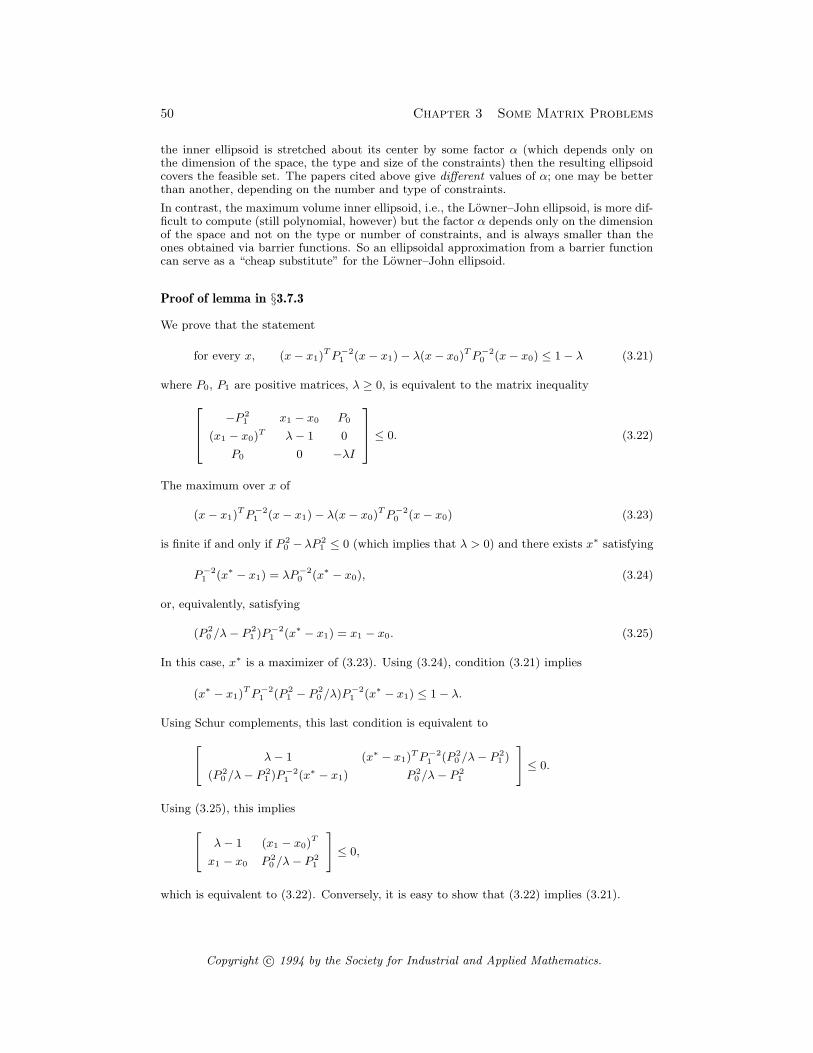
50 Chapter 3 Some Matrix Problems
the inner ellipsoid is stretched about its center by some factor α (which depends only onthe dimension of the space, the type and size of the constraints) then the resulting ellipsoidcovers the feasible set. The papers cited above give different values of α; one may be betterthan another, depending on the number and type of constraints.
In contrast, the maximum volume inner ellipsoid, i.e., the Lowner–John ellipsoid, is more dif-ficult to compute (still polynomial, however) but the factor α depends only on the dimensionof the space and not on the type or number of constraints, and is always smaller than theones obtained via barrier functions. So an ellipsoidal approximation from a barrier functioncan serve as a “cheap substitute” for the Lowner–John ellipsoid.
Proof of lemma in §3.7.3
We prove that the statement
for every x, (x− x1)TP−21 (x− x1)− λ(x− x0)TP−20 (x− x0) ≤ 1− λ (3.21)
where P0, P1 are positive matrices, λ ≥ 0, is equivalent to the matrix inequality
−P 21 x1 − x0 P0
(x1 − x0)T λ− 1 0
P0 0 −λI
≤ 0. (3.22)
The maximum over x of
(x− x1)TP−21 (x− x1)− λ(x− x0)TP−20 (x− x0) (3.23)
is finite if and only if P 20 −λP 21 ≤ 0 (which implies that λ > 0) and there exists x∗ satisfying
P−21 (x∗ − x1) = λP−20 (x∗ − x0), (3.24)
or, equivalently, satisfying
(P 20 /λ− P 21 )P−21 (x∗ − x1) = x1 − x0. (3.25)
In this case, x∗ is a maximizer of (3.23). Using (3.24), condition (3.21) implies
(x∗ − x1)TP−21 (P 21 − P 20 /λ)P−21 (x∗ − x1) ≤ 1− λ.
Using Schur complements, this last condition is equivalent to
[
λ− 1 (x∗ − x1)TP−21 (P 20 /λ− P 21 )(P 20 /λ− P 21 )P−21 (x∗ − x1) P 20 /λ− P 21
]
≤ 0.
Using (3.25), this implies
[
λ− 1 (x1 − x0)T
x1 − x0 P 20 /λ− P 21
]
≤ 0,
which is equivalent to (3.22). Conversely, it is easy to show that (3.22) implies (3.21).
Copyright c© 1994 by the Society for Industrial and Applied Mathematics.

Chapter 4
Linear Differential Inclusions
4.1 Differential Inclusions
A differential inclusion (DI) is described by:
x ∈ F (x(t), t), x(0) = x0, (4.1)
where F is a set-valued function on Rn×R+. Any x : R+ → Rn that satisfies (4.1) iscalled a solution or trajectory of the DI (4.1). Of course, there can be many solutionsof the DI (4.1). Our goal is to establish that various properties are satisfied by allsolutions of a given DI. For example, we might show that every trajectory of a givenDI converges to zero as t→∞.
By a standard result called the Relaxation Theorem, we may as well assumeF (x, t) is a convex set for every x and t. The DI given by
x ∈ CoF (x(t), t), x(0) = x0 (4.2)
is called the relaxed version of the DI (4.1). Since CoF (x(t), t) ⊇ F (x(t), t), everytrajectory of the DI (4.1) is also a trajectory of relaxed DI (4.2). Very roughly speak-ing, the Relaxation Theorem states that for many purposes the converse is true. (Seethe References for precise statements.) As a specific and simple example, it can beshown that for every DI we encounter in this book, the reachable or attainable sets ofthe DI and its relaxed version coincide, i.e., for every T ≥ 0
x(T ) | x satisfies (4.1) = x(T ) | x satisfies (4.2) .In fact we will not need the Relaxation Theorem, or rather, we will always get it
“for free”—every result we establish in the next two chapters extends immediately tothe relaxed version of the problem. The reason is that when a quadratic Lyapunovfunction is used to establish some property for the DI (4.1), then the same Lyapunovfunction establishes the property for the relaxed DI (4.2).
4.1.1 Linear differential inclusions
A linear differential inclusion (LDI) is given by
x ∈ Ωx, x(0) = x0, (4.3)
where Ω is a subset of Rn×n. We can interpret the LDI (4.3) as describing a familyof linear time-varying systems. Every trajectory of the LDI satisfies
x = A(t)x, x(0) = x0, (4.4)
51
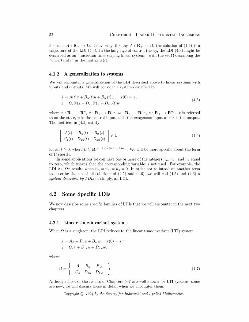
52 Chapter 4 Linear Differential Inclusions
for some A : R+ → Ω. Conversely, for any A : R+ → Ω, the solution of (4.4) is atrajectory of the LDI (4.3). In the language of control theory, the LDI (4.3) might bedescribed as an “uncertain time-varying linear system,” with the set Ω describing the“uncertainty” in the matrix A(t).
4.1.2 A generalization to systems
We will encounter a generalization of the LDI described above to linear systems withinputs and outputs. We will consider a system described by
x = A(t)x+Bu(t)u+Bw(t)w, x(0) = x0,
z = Cz(t)x+Dzu(t)u+Dzw(t)w(4.5)
where x : R+ → Rn, u : R+ → Rnu , w : R+ → Rnw , z : R+ → Rnz . x is referredto as the state, u is the control input, w is the exogenous input and z is the output.The matrices in (4.5) satisfy
[
A(t) Bu(t) Bw(t)
Cz(t) Dzu(t) Dzw(t)
]
∈ Ω. (4.6)
for all t ≥ 0, where Ω ⊆ R(n+nz)×(n+nu+nw). We will be more specific about the formof Ω shortly.
In some applications we can have one or more of the integers nu, nw, and nz equalto zero, which means that the corresponding variable is not used. For example, theLDI x ∈ Ωx results when nu = nw = nz = 0. In order not to introduce another termto describe the set of all solutions of (4.5) and (4.6), we will call (4.5) and (4.6) asystem described by LDIs or simply, an LDI.
4.2 Some Specific LDIs
We now describe some specific families of LDIs that we will encounter in the next twochapters.
4.2.1 Linear time-invariant systems
When Ω is a singleton, the LDI reduces to the linear time-invariant (LTI) system
x = Ax+Buu+Bww, x(0) = x0,
z = Czx+Dzuu+Dzww,
where
Ω =
[
A Bu Bw
Cz Dzu Dzw
]
. (4.7)
Although most of the results of Chapters 5–7 are well-known for LTI systems, someare new; we will discuss these in detail when we encounter them.
Copyright c© 1994 by the Society for Industrial and Applied Mathematics.
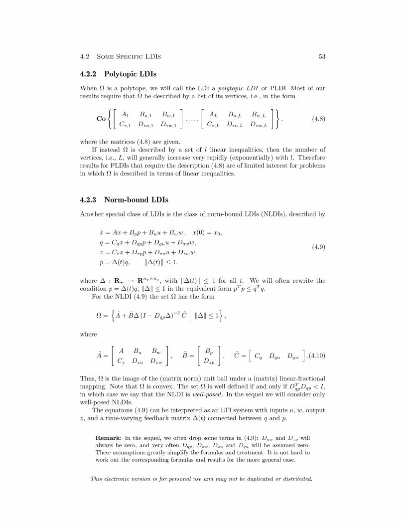
4.2 Some Specific LDIs 53
4.2.2 Polytopic LDIs
When Ω is a polytope, we will call the LDI a polytopic LDI or PLDI. Most of ourresults require that Ω be described by a list of its vertices, i.e., in the form
Co
[
A1 Bu,1 Bw,1
Cz,1 Dzu,1 Dzw,1
]
, . . . ,
[
AL Bu,L Bw,L
Cz,L Dzu,L Dzw,L
]
. (4.8)
where the matrices (4.8) are given.If instead Ω is described by a set of l linear inequalities, then the number of
vertices, i.e., L, will generally increase very rapidly (exponentially) with l. Thereforeresults for PLDIs that require the description (4.8) are of limited interest for problemsin which Ω is described in terms of linear inequalities.
4.2.3 Norm-bound LDIs
Another special class of LDIs is the class of norm-bound LDIs (NLDIs), described by
x = Ax+Bpp+Buu+Bww, x(0) = x0,
q = Cqx+Dqpp+Dquu+Dqww,
z = Czx+Dzpp+Dzuu+Dzww,
p = ∆(t)q, ‖∆(t)‖ ≤ 1.
(4.9)
where ∆ : R+ → Rnp×nq , with ‖∆(t)‖ ≤ 1 for all t. We will often rewrite thecondition p = ∆(t)q, ‖∆‖ ≤ 1 in the equivalent form pT p ≤ qT q.
For the NLDI (4.9) the set Ω has the form
Ω =
A+ B∆(I −Dqp∆)−1
C∣
∣
∣‖∆‖ ≤ 1
,
where
A =
[
A Bu Bw
Cz Dzu Dzw
]
, B =
[
Bp
Dzp
]
, C =[
Cq Dqu Dqw
]
.(4.10)
Thus, Ω is the image of the (matrix norm) unit ball under a (matrix) linear-fractionalmapping. Note that Ω is convex. The set Ω is well defined if and only if DT
qpDqp < I,in which case we say that the NLDI is well-posed . In the sequel we will consider onlywell-posed NLDIs.
The equations (4.9) can be interpreted as an LTI system with inputs u, w, outputz, and a time-varying feedback matrix ∆(t) connected between q and p.
Remark: In the sequel, we often drop some terms in (4.9): Dqw and Dzp willalways be zero, and very often Dqp, Dzw, Dzu and Dqu will be assumed zero.These assumptions greatly simplify the formulas and treatment. It is not hard towork out the corresponding formulas and results for the more general case.
This electronic version is for personal use and may not be duplicated or distributed.
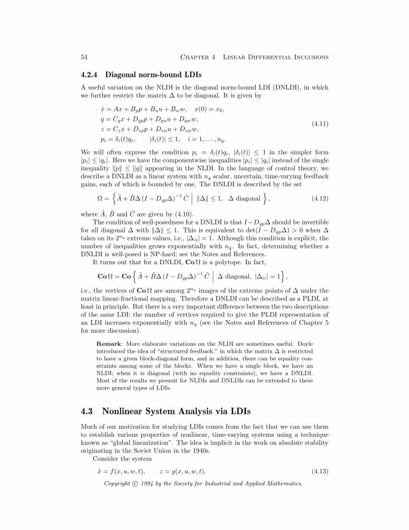
54 Chapter 4 Linear Differential Inclusions
4.2.4 Diagonal norm-bound LDIs
A useful variation on the NLDI is the diagonal norm-bound LDI (DNLDI), in whichwe further restrict the matrix ∆ to be diagonal. It is given by
x = Ax+Bpp+Buu+Bww, x(0) = x0,
q = Cqx+Dqpp+Dquu+Dqww,
z = Czx+Dzpp+Dzuu+Dzww,
pi = δi(t)qi, |δi(t)| ≤ 1, i = 1, . . . , nq.
(4.11)
We will often express the condition pi = δi(t)qi, |δi(t)| ≤ 1 in the simpler form|pi| ≤ |qi|. Here we have the componentwise inequalities |pi| ≤ |qi| instead of the singleinequality ‖p‖ ≤ ‖q‖ appearing in the NLDI. In the language of control theory, wedescribe a DNLDI as a linear system with nq scalar, uncertain, time-varying feedbackgains, each of which is bounded by one. The DNLDI is described by the set
Ω =
A+ B∆(I −Dqp∆)−1
C∣
∣
∣‖∆‖ ≤ 1, ∆ diagonal
, (4.12)
where A, B and C are given by (4.10).The condition of well-posedness for a DNLDI is that I−Dqp∆ should be invertible
for all diagonal ∆ with ‖∆‖ ≤ 1. This is equivalent to det(I − Dqp∆) > 0 when ∆takes on its 2nq extreme values, i.e., |∆ii| = 1. Although this condition is explicit, thenumber of inequalities grows exponentially with nq. In fact, determining whether aDNLDI is well-posed is NP-hard; see the Notes and References.
It turns out that for a DNLDI, CoΩ is a polytope. In fact,
CoΩ = Co
A+ B∆(I −Dqp∆)−1
C∣
∣
∣ ∆ diagonal, |∆ii| = 1
,
i.e., the vertices of CoΩ are among 2nq images of the extreme points of ∆ under thematrix linear-fractional mapping. Therefore a DNLDI can be described as a PLDI, atleast in principle. But there is a very important difference between the two descriptionsof the same LDI: the number of vertices required to give the PLDI representation ofan LDI increases exponentially with nq (see the Notes and References of Chapter 5for more discussion).
Remark: More elaborate variations on the NLDI are sometimes useful. Doyleintroduced the idea of “structured feedback,” in which the matrix ∆ is restrictedto have a given block-diagonal form, and in addition, there can be equality con-straints among some of the blocks. When we have a single block, we have anNLDI; when it is diagonal (with no equality constraints), we have a DNLDI.Most of the results we present for NLDIs and DNLDIs can be extended to thesemore general types of LDIs.
4.3 Nonlinear System Analysis via LDIs
Much of our motivation for studying LDIs comes from the fact that we can use themto establish various properties of nonlinear, time-varying systems using a techniqueknown as “global linearization”. The idea is implicit in the work on absolute stabilityoriginating in the Soviet Union in the 1940s.
Consider the system
x = f(x, u, w, t), z = g(x, u, w, t). (4.13)
Copyright c© 1994 by the Society for Industrial and Applied Mathematics.
4.3 Nonlinear System Analysis via LDIs 55
Suppose that for each x, u, w, and t there is a matrix G(x, u, w, t) ∈ Ω such that
[
f(x, u, w, t)
g(x, u, w, t)
]
= G(x, u, w, t)
x
u
w
(4.14)
where Ω ⊆ R(n+nz)×(n+nu+nw). Then of course every trajectory of the nonlinearsystem (4.13) is also a trajectory of the LDI defined by Ω. If we can prove that everytrajectory of the LDI defined by Ω has some property (e.g., converges to zero), thena fortiori we have proved that every trajectory of the nonlinear system (4.13) has thisproperty.
4.3.1 A derivative condition
Conditions that guarantee the existence of such a G are f(0, 0, 0, 0) = 0, g(0, 0, 0, 0) =0, and
∂f
∂x
∂f
∂u
∂f
∂w
∂g
∂x
∂g
∂u
∂g
∂w
∈ Ω for all x, u, w, t. (4.15)
In fact we can make a stronger statement that links the difference between a pairof trajectories of the nonlinear system and the trajectories of the LDI given by Ω.Suppose we have (4.15) but not necessarily f(0, 0, 0, 0) = 0, g(0, 0, 0, 0) = 0. Then forany pair of trajectories (x,w, z) and (x, w, z) we have
[
x− ˙x
z − z
]
∈ CoΩ
x− x
u− u
w − w
,
i.e., (x− x, w − w, z − z) is a trajectory of the LDI given by CoΩ.These results follow from a simple extension of the mean-value theorem: if φ :
Rn → Rn satisfies
∂φ
∂x∈ Ω
throughout Rn, then for any x and x we have
φ(x)− φ(x) ∈ CoΩ(x− x). (4.16)
To see this, let c ∈ Rn. By the mean-value theorem we have
cT (φ(x)− φ(x)) = cT∂φ
∂x(ζ)(x− x)
for some ζ that lies on the line segment between x and x. Since by assumption
∂φ
∂x(ζ) ∈ Ω,
we conclude that
cT (φ(x)− φ(x)) ≤ sup
A ∈ CoΩ
cTA(x− x).
Since c was arbitrary, we see that φ(x)− φ(x) is in every half-space that contains theconvex set CoΩ(x− x), which proves (4.16).
This electronic version is for personal use and may not be duplicated or distributed.
56 Chapter 4 Linear Differential Inclusions
4.3.2 Sector conditions
Sometimes the nonlinear system (4.13) can be expressed in the form
x = Ax+Bpp+Buu+Bww,
q = Cqx+Dqpp+Dquu+Dqww,
z = Czx+Dzpp+Dzuu+Dzww,
pi = φi(qi, t), i = 1, . . . , nq,
(4.17)
where φi : R×R+ → R satisfy the sector conditions
αiq2 ≤ qφi(q, t) ≤ βiq
2
for all q and t ≥ 0, where αi and βi are given. In words, the system consists of a linearpart together with nq time-varying sector-bounded scalar nonlinearities.
The variables pi and qi can be eliminated from (4.17) provided the matrix I−Dqp∆is nonsingular for all diagonal ∆ with αi ≤ ∆ii ≤ βi. In this case, we say the systemis well-posed.
Assume now that the system (4.17) is well-posed, and let (4.13) be the equationsobtained by eliminating the variables p and q. Define
Ω =
A+ B∆(I −Dqp∆)−1
C∣
∣
∣ ∆ diagonal, ∆ii ∈ [αi, βi]
,
where A, B and C are given by (4.10). Then, the condition (4.14) holds.
Notes and References
Differential inclusions
The books by Aubin and Cellina [AC84], Kisielewicz [Kis91], and the classic text by Filip-pov [Fil88] cover the theory of differential inclusions. See also the article by Roxin [Rox65]and references therein. Background material, e.g., set-valued analysis, can be found in thebook by Aubin and Frankowska [AF90].
The term linear differential inclusion is a bit misleading, since LDIs do not enjoy any particu-lar linearity or superposition properties. We use the term only to point out the interpretationas an uncertain time-varying linear system. Many authors refer to LDIs using some subsetof the phrase “uncertain linear time-varying system”. A more accurate term, suggested tous and used by A. Filippov and E. Pyatnitskii, is selector-linear differential inclusion.
PLDIs come up in several articles on control theory, e.g., [MP89, KP87a, KP87b, BY89].
Integral quadratic constraints
The pointwise quadratic constraint p(t)T p(t) ≤ q(t)T q(t) that occur in NLDIs can be gener-
alized to the integral quadratic constraint∫ t
0pT p dτ ≤
∫ t
0qT q dτ ; see §8.2 and §8.3.
Global linearization
The idea of replacing a nonlinear system by a time-varying linear system can be found in Liuet al. [Liu68, LSL69]. They call this approach global linearization. Of course, approximatingthe set of trajectories of a nonlinear system via LDIs can be very conservative, i.e., there aremany trajectories of the LDI that are not trajectories of the nonlinear system. We will seein Chapter 8 how this conservatism can be reduced in some special cases.
The idea of global linearization is implicit in the early Soviet literature on the absolutestability problem, e.g., Lur’e and Postnikov [LP44, Lur57] and Popov [Pop73].
Copyright c© 1994 by the Society for Industrial and Applied Mathematics.

Notes and References 57
Modeling systems as PLDIs
One of the key issues in robust control theory is how to model or measure plant “uncertainty”or “variation”. We propose a simple method that should work well in some cases. At theleast, the method is extremely simple and natural.
Suppose we have a real system that is fairly well modeled as a linear system. We collectmany sets of input/output measurements, obtained at different times, under different op-erating conditions, or perhaps from different instances of the system (e.g., different unitsfrom a manufacturing run). It is important that we have data sets from enough plants orplant conditions to characterize or at least give some idea of the plant variation that can beexpected.
For each data set we develop a linear system model of the plant. To simplify the problemwe will assume that the state in this model is accessible, so the different models refer to thesame state vector. These models should be fairly close, but of course not exactly the same.We might find for example that the transfer matrices of these models at s = 0 differ by about10%, but at high frequencies they differ considerably more. More importantly, this collectionof models contains information about the “structure” of the plant variation.
We propose to model the system as a PLDI with the vertices given by the measured orestimated linear system models. In other words, we model the plant as a time-varying linearsystem, with system matrices that can jump around among any of the models we estimated.It seems reasonable to conjecture that a controller that works well with this PLDI is likelyto work well when connected to the real system. Such controllers can be designed by themethods described in Chapter 7.
Well-posedness of DNLDIs
See [BY89] for a proof that a DNLDI is well-posed if and only if det(I−Dqp∆) > 0 for every∆ with |∆ii| = 1; the idea behind this proof can be traced back to Zadeh and Desoer [ZD63,§9.17]; see also [Sae86]. An equivalent condition is in terms of P0 matrices (a matrix is P0if every principal minor is nonnegative; see [FP62, FP66, FP67]): A DNLDI is well-posed ifand only if I +Dqp is invertible, and (I +Dqp)
−1(I −Dqp) is a P0 matrix [Gha90]. Anotherequivalent condition is that (I + Dqp, I − Dqp) is a W0 pair (see [Wil70]). The problemof determining whether a general matrix is P0 is thought to be very difficult, i.e., of highcomplexity [CPS92, p149].
Standard branch-and-bound techniques can be applied to the problem of determining well-posedness of DNLDIs; see for example [Sd86, GS88, SP89, BBB91, BB92]. Of course thesemethods have no theoretical advantage over simply checking that the 2nq determinants arepositive. But in practice they may be more efficient, especially when used with computation-ally cheap sufficient conditions (see below).
There are several sufficient conditions for well-posedness of a DNLDI that can be checked inpolynomial-time. Fan, Tits, and Doyle [FTD91] show that if the LMI
DTqpPDqp < P, P diagonal, P > 0, (4.18)
is feasible, then the DNLDI is well-posed. Condition (4.18) is equivalent to the existence of adiagonal (scaling) matrix R such that ‖RDqpR
−1‖ < 1. In [FTD91], the authors also give asufficient condition for well-posedness of more general “structured” LDIs, e.g., when equalityconstraints are imposed on the matrix ∆ in (4.11). These conditions can also be obtainedusing the S-procedure; see [Fer93].
Representing DNLDIs as PLDIs
For a well-posed DNLDI, CoΩ is a polytope, which means that the DNLDI (4.12) can alsobe represented as a PLDI. More specifically, we have
CoΩ = Co
A+ B∆(I −Dqp∆)−1 C∣
∣ ∆ diagonal, |∆ii| = 1
,
This electronic version is for personal use and may not be duplicated or distributed.
58 Chapter 4 Linear Differential Inclusions
where A, B and C are given by (4.10). Note that the set on the right-hand side is a polytopewith at most 2nq vertices. We now prove this result.
Define
K =
A+ B∆(I −Dqp∆)−1 C∣
∣ ∆ diagonal, |∆ii| = 1
,
which is a set containing at most 2nq points. By definition
CoΩ = Co
A+ B∆(I −Dqp∆)−1 C∣
∣ ∆ diagonal, |∆ii| ≤ 1
.
Clearly we have CoΩ ⊇ CoK. We will now show that every extreme point of CoΩ iscontained in CoK, which will imply that CoK ⊇ CoΩ, completing the proof.
Let Wext be an extreme point of CoΩ. Then there exists a linear function ψ such that Wextis the unique maximizer of ψ over CoΩ. In fact, Wext ∈ Ω, since otherwise, the half-spaceW | ψ(W ) < ψ(Wext)− ε, where ε > 0 is sufficiently small, contains Ω but not Wext, whichcontradicts Wext ∈ CoΩ.
Now, for W ∈ Ω, ψ(W ) is a bounded linear-fractional function of the first diagonal entry∆11 of ∆, for fixed ∆22, . . . ,∆nqnq , i.e., it equals (a+ b∆11)/(c+ d∆11) for some a, b, c andd. Moreover, the denominator c + d∆11 is nonzero for ∆11 ∈ [−1, 1], since the DNLDI iswell-posed. Therefore, for every fixed ∆22, . . . ,∆nqnq , the function ψ achieves a maximum atan extreme value of ∆11, i.e., ∆11 = ±1. Extending this argument to ∆22, . . . ,∆nqnq leads
us to the following conclusion: Wext = A + BS (I −DqpS)−1 C, where S satisfies Sii = ±1.
In other words, Wext ∈ CoK, which concludes our proof.
We have already noted that the description of a DNLDI as a PLDI will be much larger thanits description as a DNLDI; see the Notes and References of Chapter 5, and also [BY89] and[PS82, KP87a, Kam83].
Approximating PLDIs by NLDIs
It is often useful to conservatively approximate a PLDI as an NLDI. One reason, amongmany, is the potentially much smaller size of the description as an NLDI compared to thedescription of the PLDI. We consider the PLDI
x = A(t)x, A(t) ∈ ΩPLDI∆= Co A1, . . . , AL , (4.19)
with x(t) ∈ Rn, and the NLDI
x = (A+Bp∆(t)Cq)x, ‖∆(t)‖ ≤ 1, (4.20)
with associated set ΩNLDI∆= A+Bp∆Cq | ‖∆‖ ≤ 1. Our goal is to find A, Bp, and Cq
such that ΩPLDI ⊆ ΩNLDI with the set ΩNLDI as small as possible in some appropriate sense.This will give an efficient outer approximation of the PLDI (4.19) by the NLDI (4.20). SinceΩPLDI ⊆ ΩNLDI implies that every trajectory of the PLDI is a trajectory of the NLDI, everyresult we establish for all trajectories of the NLDI holds for all trajectories of the PLDI. ForL very large, it is much easier to work with the NLDI than the PLDI.
For simplicity, we will only consider the case with Bp ∈ Rn×n and invertible. Evidently thereis substantial redundancy in our representation of the NLDI (4.20): We can replace Bp byαBp and Cq by Cq/α where α 6= 0. (We can also replace Bp and Cq with BpU and V Cq
where U and V are any orthogonal matrices, without affecting the set ΩNLDI, but we willnot use this fact.)
We have ΩPLDI ⊆ ΩNLDI if for every ξ and k = 1, . . . , L, there exists π such that
Bpπ = (Ak −A)ξ, πTπ ≤ ξTCTq Cqξ.
Copyright c© 1994 by the Society for Industrial and Applied Mathematics.
Notes and References 59
This yields the equivalent condition
(Ak −A)TB−Tp B−1p (Ak −A) ≤ CTq Cq, k = 1, . . . , L,
which, in turn, is equivalent to
BpBTp > 0,
[
CTq Cq (Ak −A)T
Ak −A BpBTp
]
≥ 0, k = 1, . . . , L.
Introducing new variables V = CTq Cq and W = BpB
Tp , we get the equivalent LMI in A, V
and W
W > 0,
[
V (Ak −A)T
Ak −A W
]
≥ 0, k = 1, . . . , L. (4.21)
Thus we have ΩPLDI ⊆ ΩNLDI if condition (4.21) holds.
There are several ways to minimize the size of ΩNLDI ⊇ ΩPLDI. The most obvious is tominimize TrV + TrW subject to (4.21), which is an EVP in A, V and W . This objectiveis clearly related to several measures of the size of ΩNLDI, but we do not know of any simpleinterpretation.
We can formulate the problem of minimizing the diameter of ΩNLDI as an EVP. We define thediameter of a set Ω ⊆ Rn×n as max ‖F −G‖ | F, G ∈ Ω. The diameter of ΩNLDI is equal
to 2√
λmax(V )λmax(W ). We can exploit the scaling redundancy in Cq to assume without lossof generality that λmax(V ) ≤ 1, and then minimize λmax(W ) subject to (4.21) and V ≤ I,which is an EVP. It can be shown that the resulting optimal V opt satisfies λmax(V
opt) = 1,so that we have in fact minimized the diameter of ΩNLDI subject to ΩPLDI ⊆ ΩNLDI.
This electronic version is for personal use and may not be duplicated or distributed.


Chapter 5
Analysis of LDIs:State Properties
In this chapter we consider properties of the state x of the LDI
x = A(t)x, A(t) ∈ Ω, (5.1)
where Ω ⊆ Rn×n has one of four forms:
• LTI systems: LTI systems are described by x = Ax.
• Polytopic LDIs: PLDIs are described by x = A(t)x, A(t) ∈ Co A1, . . . , AL.
• Norm-bound LDIs: NLDIs are described by
x = Ax+Bpp, q = Cqx+Dqpp, p = ∆(t)q, ‖∆(t)‖ ≤ 1,
which we will rewrite as
x = Ax+Bpp, pT p ≤ (Cqx+Dqpp)T (Cqx+Dqpp). (5.2)
We assume well-posedness, i.e., ‖Dqp‖ < 1.
• Diagonal Norm-bound LDIs: DNLDIs are described by
x = Ax+Bpp, q = Cqx+Dqpp,
pi = δi(t)qi, |δi(t)| ≤ 1, i = 1, . . . , nq.(5.3)
which can be rewritten as
x = Ax+Bpp, q = Cqx+Dqpp, |pi| ≤ |qi|, i = 1, . . . , nq.
Again, we assume well-posedness.
5.1 Quadratic Stability
We first study stability of the LDI (5.1), that is, we ask whether all trajectories ofsystem (5.1) converge to zero as t→∞. A sufficient condition for this is the existenceof a quadratic function V (ξ) = ξTPξ, P > 0 that decreases along every nonzerotrajectory of (5.1). If there exists such a P , we say the LDI (5.1) is quadratically
stable and we call V a quadratic Lyapunov function.
61
62 Chapter 5 Analysis of LDIs: State Properties
Since
d
dtV (x) = xT
(
A(t)TP + PA(t))
x,
a necessary and sufficient condition for quadratic stability of system (5.1) is
P > 0, ATP + PA < 0 for all A ∈ Ω. (5.4)
Multiplying the second inequality in (5.4) on the left and right by P−1, and defininga new variable Q = P−1, we may rewrite (5.4) as
Q > 0, QAT +AQ < 0 for all A ∈ Ω. (5.5)
This dual inequality is an equivalent condition for quadratic stability. We now showthat conditions for quadratic stability for LTI systems, PLDIs, and NLDIs can beexpressed in terms of LMIs.
• LTI systems: Condition (5.4) becomes
P > 0, ATP + PA < 0. (5.6)
Therefore, checking quadratic stability for an LTI system is an LMIP in the variableP . This is precisely the (necessary and sufficient) Lyapunov stability criterion for LTIsystems. (In other words, a linear system is stable if and only if it is quadratically sta-ble.) Alternatively, using (5.5), stability of LTI systems is equivalent to the existenceof Q satisfying the LMI
Q > 0, AQ+QAT < 0. (5.7)
Of course, each of these (very special) LMIPs can be solved analytically by solving aLyapunov equation (see §1.2 and §2.7).
• Polytopic LDIs: Condition (5.4) is equivalent to
P > 0, ATi P + PAi < 0, i = 1, . . . , L. (5.8)
Thus, determining quadratic stability for PLDIs is an LMIP in the variable P . Thedual condition (5.5) is equivalent to the LMI in the variable Q
Q > 0, QATi +AiQ < 0, i = 1, . . . , L. (5.9)
• Norm-bound LDIs: Condition (5.4) is equivalent to P > 0 and
[
ξ
π
]T [
ATP + PA PBp
BTp P 0
][
ξ
π
]
< 0 (5.10)
for all nonzero ξ satisfying
[
ξ
π
]T
−CTq Cq −CT
q Dqp
−DTqpCq I −DT
qpDqp
[
ξ
π
]
≤ 0. (5.11)
In order to apply the S-procedure we show that the set
A = (ξ, π) | ξ 6= 0, (5.11)Copyright c© 1994 by the Society for Industrial and Applied Mathematics.
5.1 Quadratic Stability 63
equals the set
B = (ξ, π) | (ξ, π) 6= 0, (5.11) .
It suffices to show that (ξ, π) | ξ = 0, π 6= 0, (5.11) = ∅. But this is immediate:If π 6= 0, then condition (5.11) cannot hold without having ξ 6= 0, since I−DT
qpDqp > 0.Therefore, the condition that dV (x)/dt < 0 for all nonzero trajectories is equivalentto (5.10) being satisfied for any nonzero (ξ, π) satisfying (5.11). (This argument recursthroughout this chapter and will not be repeated.) Using the S-procedure, we findthat quadratic stability of (5.2) is equivalent to the existence of P and λ satisfying
P > 0, λ ≥ 0,
ATP + PA+ λCTq Cq PBp + λCT
q Dqp
(PBp + λCTq Dqp)
T −λ(I −DTqpDqp)
< 0.(5.12)
Thus, determining quadratic stability of an NLDI is an LMIP. Since LMI (5.12) impliesthat λ > 0, we may, by defining P = P/λ, obtain an equivalent condition
P > 0,
AT P + PA+ CTq Cq PBp + CT
q Dqp
(PBp + CTq Dqp)
T −(I −DTqpDqp)
< 0, (5.13)
an LMI in the variable P . Thus, quadratic stability of the NLDI has the frequency-domain interpretation that the H∞ norm of the LTI system
x = Ax+Bpp, q = Cqx+Dqpp
is less than one.With the new variables Q = P−1, µ = 1/λ, quadratic stability of NLDIs is also
equivalent to the existence of µ and Q satisfying the LMI
µ ≥ 0, Q > 0,
[
AQ+QAT + µBpBTp µBpD
Tqp +QCT
q
(µBpDTqp +QCT
q )T −µ(I −DqpD
Tqp)
]
< 0.(5.14)
Remark: Note that our assumption of well-posedness is in fact incorporated inthe LMI (5.12) since it implies I − DqpD
Tqp > 0. Therefore the NLDI (5.2) is
well-posed and quadratically stable if and only if the LMIP (5.12) has a solution.
In the remainder of this chapter we will assume that Dqp in (5.2) is zero; thereader should bear in mind that all the following results hold for nonzero Dqp as well.
• Diagonal Norm-bound LDIs: For the DNLDI (5.3), we can obtain only asufficient condition for quadratic stability. The condition dV (x)/dt < 0 for all nonzerotrajectories is equivalent to
ξT (ATP + PA)ξ + 2ξTPBpπ < 0
for all nonzero (ξ, π) satisfying
π2i ≤ (Cq,iξ +Dqp,iπ)T(Cq,iξ +Dqp,iπ) , i = 1, . . . , L,
This electronic version is for personal use and may not be duplicated or distributed.
64 Chapter 5 Analysis of LDIs: State Properties
where we have used Cq,i and Dqp,i to denote the ith rows of Cq and Dqp respec-tively. Using the S-procedure, we see that this condition is implied by the existenceof nonnegative λ1, . . . , λnq
such that
ξT (ATP + PA)ξ + 2ξTPBpπ
+
L∑
i=1
λi
(
(Cq,iξ +Dqp,iπ)T(Cq,iξ +Dqp,iπ)− π2i
)
< 0
for all nonzero (ξ, π). With Λ = diag(λ, . . . , λnq), this is equivalent to
[
ATP + PA+ CTq ΛCq PBp + CT
q ΛDqp
BTp P +DT
qpΛCq DTqpΛDqp − Λ
]
< 0. (5.15)
Therefore, if there exist P > 0 and diagonal Λ ≥ 0 satisfying (5.15), then theDNLDI (5.3) is quadratically stable. Checking this sufficient condition for quadraticstability is an LMIP. Note that from (5.15), we must have Λ > 0.
Equivalently, quadratic stability is implied by the existence of Q > 0, M =diag(µ1, . . . , µnq
) > 0 satisfying the LMI[
AQ+QAT +BpMBTp QCT
q +BpMDTqp
CqQ+DqpMBTp −M +DqpMDT
qp
]
< 0, (5.16)
another LMIP.
Remark: Quadratic stability of a DNLDI via the S-procedure has a simplefrequency-domain interpretation. Denoting by H the transfer matrix H(s) =Dqp + Cq(sI − A)−1Bp, and assuming (A,Bp, Cq) is minimal, quadratic stabil-ity is equivalent to the fact that, for some diagonal, positive-definite matrix Λ,‖Λ1/2HΛ−1/2‖∞ < 1. Λ−1/2 can then be interpreted as a scaling. (See the Notesand References for more details on the connection between the S-procedure andscaling.)
Remark: Here too our assumption of well-posedness is in fact incorporatedin the LMI (5.15) or (5.16). The bottom right block is precisely the sufficientcondition for well-posedness mentioned on page 57. Therefore the DNLDI (5.2)is well-posed and quadratically stable if the LMI (5.15) or (5.16) is feasible.
Note the similarity between the corresponding LMIs for the NLDI and the DNLDI;the only difference is that the diagonal matrix appearing in the LMI associated withthe DNLDI is fixed as the scaled identity matrix in the LMI associated with the NLDI.In general it is straightforward to derive the corresponding (sufficient) condition forDNLDIs from the result for NLDIs. In the remainder of the book, we will often restrictour attention to NLDIs, and pay only occasional attention to DNLDIs; we leave tothe reader the task of generalizing all the results for NLDIs to DNLDIs.
Remark: An LTI system is stable if and only if it is quadratically stable. Formore general LDIs, however, stability does not imply quadratic stability (see theNotes and References at the end of this chapter). It is true that an LDI isstable if and only if there exists a convex Lyapunov function that proves it; seethe Notes and References.
Copyright c© 1994 by the Society for Industrial and Applied Mathematics.
5.1 Quadratic Stability 65
5.1.1 Coordinate transformations
We can give another interpretation of quadratic stability in terms of state-space coor-dinate transformations. Consider the change of coordinates x = T x, where detT 6= 0.In the new coordinate system, (5.1) is described by the matrix A(t) = T−1A(t)T .We ask the question: Does there exist T such that in the new coordinate system, all(nonzero) trajectories of the LDI are always decreasing in norm, i.e., d‖x‖/dt < 0?It is easy to show that this is true if and only if there exists a quadratic Lyapunovfunction V (ξ) = ξTPξ for the LDI, in which case we can take any T with TT T = P−1,for example, T = P−1/2 (these T ’s are all related by right orthogonal matrix multi-plication). With this interpretation, it is natural to seek a coordinate transformationmatrix T that makes all nonzero trajectories decreasing in norm, and has the small-est possible condition number κ(T ). This turns out to be an EVP for LTI systems,polytopic and norm-bound LDIs.
To see this, let P = T−TT−1, so that κ(T )2 = κ(P ). Minimizing the conditionnumber of T subject to the requirement that d‖x‖/dt < 0 for all nonzero trajectories isthen equivalent to minimizing the condition number of P subject to d(xTPx)/dt < 0.(Any T with TT T = P−1opt where Popt is an optimal solution, is optimal for the originalproblem.) For each of our systems (LTI systems, PLDIs and NLDIs), the change ofcoordinates with smallest condition number is obtained by solving the following EVPs:
• LTI systems: The EVP in the variables P and η is
minimize η
subject to (5.6), I ≤ P ≤ ηI
(In this formulation, we have taken advantage of the homogeneity of the LMI (5.6) inthe variable P .)
• Polytopic LDIs: The EVP in the variables P and η is
minimize η
subject to (5.8), I ≤ P ≤ ηI
• Norm-bound LDIs: The EVP in the variables P , η and λ is
minimize η
subject to (5.12), I ≤ P ≤ ηI
5.1.2 Quadratic stability margins
Quadratic stability margins give a measure of how much the set Ω can be expandedabout some center with the LDI remaining quadratically stable.
• Polytopic LDIs: For the PLDI
x = (A0 +A(t))x, A(t) ∈ α Co A1, . . . , AL ,
we define the quadratic stability margin as the largest nonnegative α for which it isquadratically stable. This quantity is computed by solving the following GEVP in P
This electronic version is for personal use and may not be duplicated or distributed.
66 Chapter 5 Analysis of LDIs: State Properties
and α:
maximize α
subject to P > 0, α ≥ 0,
AT0 P + PA0 + α
(
ATi P + PAi
)
< 0, i = 1, . . . , L
• Norm-bound LDIs: The quadratic stability margin of the system
x = Ax+Bpp, pT p ≤ α2xTCTq Cqx,
is defined as the largest α ≥ 0 for which the system is quadratically stable, and iscomputed by solving the GEVP in P , λ and β = α2:
maximize β
subject to P > 0, β ≥ 0,
[
ATP + PA+ βλCTq Cq PBp
BTp P −λI
]
< 0
Defining P = P/λ, we get an equivalent EVP in P and β:
maximize β
subject to P > 0, β ≥ 0,
[
AT P + PA+ βCTq Cq PBp
BTp P −I
]
< 0
Remark: The quadratic stability margin obtained by solving this EVP is just1/‖Cq(sI −A)−1Bp‖∞.
5.1.3 Decay rate
The decay rate (or largest Lyapunov exponent) of the LDI (5.1) is defined to be thelargest α such that
limt→∞
eαt‖x(t)‖ = 0
holds for all trajectories x. Equivalently, the decay rate is the supremum of
lim inft→∞
− log ‖x(t)‖t
over all nonzero trajectories. (Stability corresponds to positive decay rate.)We can use the quadratic Lyapunov function V (ξ) = ξTPξ to establish a lower
bound on the decay rate of the LDI (5.1). If dV (x)/dt ≤ −2αV (x) for all trajectories,then V (x(t)) ≤ V (x(0))e−2αt, so that ‖x(t)‖ ≤ e−αtκ(P )1/2‖x(0)‖ for all trajectories,and therefore the decay rate of the LDI (5.1) is at least α.
• LTI systems: The condition that dV (x)/dt ≤ −2αV (x) for all trajectories isequivalent to
ATP + PA+ 2αP ≤ 0. (5.17)
Therefore, the largest lower bound on the decay rate that we can find using a quadraticLyapunov function can be found by solving the following GEVP in P and α:
maximize α
subject to P > 0, (5.17)(5.18)
Copyright c© 1994 by the Society for Industrial and Applied Mathematics.
5.1 Quadratic Stability 67
This lower bound is sharp, i.e., the optimal value of the GEVP (5.18) is the decay rateof the LTI system (which is the stability degree of A, i.e., negative of the maximumreal part of the eigenvalues of A).
As an alternate condition, there exists a quadratic Lyapunov function provingthat the decay rate is at least α if and only if there exists Q satisfying the LMI
Q > 0, AQ+QAT + 2αQ ≤ 0. (5.19)
• Polytopic LDIs: The condition that dV (x)/dt ≤ −2αV (x) for all trajectories isequivalent to the LMI
ATi P + PAi + 2αP ≤ 0, i = 1, . . . , L. (5.20)
Therefore, the largest lower bound on the decay rate provable via quadratic Lyapunovfunctions is obtained by maximizing α subject to (5.20) and P > 0. This is a GEVPin P and α.
As an alternate condition, there exists a quadratic Lyapunov function provingthat the decay rate is at least α if and only if there exists Q satisfying the LMI
Q > 0, AiQ+QATi + 2αQ ≤ 0, i = 1, . . . , L. (5.21)
• Norm-bound LDIs: Applying the S-procedure, the condition that dV (x)/dt ≤−2αV (x) for all trajectories is equivalent to the existence of λ ≥ 0 such that
[
ATP + PA+ λCTq Cq + 2αP PBp
BTp P −λI
]
≤ 0. (5.22)
Therefore, we obtain the largest lower bound on the decay rate of (5.2) by maximizingα over the variables α, P and λ, subject to P > 0, λ ≥ 0 and (5.22), a GEVP.
The lower bound has a simple frequency-domain interpretation: Define the α-shifted H∞ norm of the system by
‖H‖∞,α∆= sup ‖H(s)‖ | Re s > −α .
Then the optimal value of the GEVP is equal to the largest α such that ‖H‖∞,α < 1.This can be seen by rewriting (5.22) as
[
(A+ αI)TP + P (A+ αI) + λCT
q Cq PBp
BTp P −λI
]
≤ 0,
and noting that the H∞ norm of the system (A+ αI,Bp, Cq) equals ‖H‖∞,α.An alternate necessary and sufficient condition for the existence of a quadratic
Lyapunov function proving that the decay rate of (5.2) is at least α is that thereexists Q and µ satisfying the LMI
Q > 0, µ ≥ 0,
[
AQ+QAT + µBpBTp + 2αQ QCT
q
CqQ −µI
]
≤ 0.(5.23)
This electronic version is for personal use and may not be duplicated or distributed.
68 Chapter 5 Analysis of LDIs: State Properties
5.2 Invariant Ellipsoids
Quadratic stability can also be interpreted in terms of invariant ellipsoids. For Q > 0,let E denote the ellipsoid centered at the origin
E =
ξ ∈ Rn∣
∣ ξTQ−1ξ ≤ 1
.
The ellipsoid E is said to be invariant for the LDI (5.1) if for every trajectory x of theLDI, x(t0) ∈ E implies x(t) ∈ E for all t ≥ t0. It is easily shown that this is the caseif and only if Q satisfies
QAT +AQ ≤ 0, for all A ∈ Ω,
or equivalently,
ATP + PA ≤ 0, for all A ∈ Ω, (5.24)
where P = Q−1. Thus, for LTI systems, PLDIs and NLDIs, invariance of E is charac-terized by LMIs in Q or P , its inverse.
Remark: Condition (5.24) is just the nonstrict version of condition (5.4).
• LTI systems: The corresponding LMI in P is
P > 0, ATP + PA ≤ 0, (5.25)
and the LMI in Q is
Q > 0, AQ+ PAT ≤ 0, (5.26)
• Polytopic LDIs: The corresponding LMI in P is
P > 0, ATi P + PAi ≤ 0, i = 1, . . . , L, (5.27)
and the LMI in Q is
Q > 0, QATi +AiQ ≤ 0, i = 1, . . . , L. (5.28)
• Norm-bound LDIs: Applying the S-procedure, invariance of the ellipsoid E isequivalent to the existence of λ such that
P > 0, λ ≥ 0,
ATP + PA+ λCTq Cq PBp + λCT
q Dqp
(PBp + λCTq Dqp)
T −λ(I −DTqpDqp)
≤ 0.(5.29)
Invariance of the ellipsoid E is equivalent to the existence of µ such that
µ ≥ 0, Q > 0, and
[
AQ+QAT + µBpBTp µBpD
Tqp +QCT
q
(µBpDTqp +QCT
q )T −µ(I −DqpD
Tqp)
]
≤ 0.(5.30)
In summary, the condition that E be an invariant ellipsoid can be expressed ineach case as an LMI in Q or its inverse P .
Copyright c© 1994 by the Society for Industrial and Applied Mathematics.
5.2 Invariant Ellipsoids 69
5.2.1 Smallest invariant ellipsoid containing a polytope
Consider a polytope described by its vertices, P = Cov1, . . . , vp. The ellipsoid Econtains the polytope P if and only if
vTj Q−1vj ≤ 1, j = 1, . . . , p.
This condition may be expressed as an LMI in Q[
1 vTjvj Q
]
≥ 0, j = 1, . . . , p, (5.31)
or as an LMI in P = Q−1 as
vTj Pvj ≤ 1, j = 1, . . . , p. (5.32)
Minimum volume
The volume of E is, up to a constant that depends on n,√detQ. We can minimize
this volume by solving appropriate CPs.
• LTI systems: The CP in P is
minimize log detP−1
subject to (5.25), (5.32)
• Polytopic LDIs: The CP in P is
minimize log detP−1
subject to (5.27), (5.32)(5.33)
• Norm-bound LDIs: The CP in P and λ is
minimize log detP−1
subject to (5.29), (5.32)
Minimum diameter
The diameter of the ellipsoid E is 2√
λmax(Q). We can minimize this quantity bysolving appropriate EVPs.
• LTI systems: The EVP in the variables Q and λ is
minimize λ
subject to (5.26), (5.31), Q ≤ λI
• Polytopic LDIs: The EVP in Q and λ is
minimize λ
subject to (5.28), (5.31), Q ≤ λI(5.34)
• Norm-bound LDIs: The EVP in Q, λ and µ is
minimize λ
subject to (5.30), (5.31), Q ≤ λI
This electronic version is for personal use and may not be duplicated or distributed.

70 Chapter 5 Analysis of LDIs: State Properties
Remark: These results have the following use. The polytope P represents ourknowledge of the state at time t0, i.e., x(t0) ∈ P (this knowledge may reflectmeasurements or prior assumptions). An invariant ellipsoid E containing P thengives a bound on the state for t ≥ t0, i.e., we can guarantee that x(t) ∈ E for allt ≥ t0.
5.2.2 Largest invariant ellipsoid contained in a polytope
We now consider a polytope described by linear inequalities:
P =
ξ ∈ Rn∣
∣ aTk ξ ≤ 1, k = 1, . . . , q
.
The ellipsoid E is contained in the polytope P if and only if
max
aTk ξ | ξ ∈ E
≤ 1, k = 1, . . . , q.
This is equivalent to
aTkQak ≤ 1, k = 1, . . . , q, (5.35)
which is a set of linear inequalities in Q. The maximum volume of invariant ellipsoidscontained in P can be found by solving CPs:
• LTI systems: For LTI systems, the CP in the variable Q is
minimize log detQ−1
subject to (5.26), (5.35)
(Since the volume of E is, up to a constant,√detQ, minimizing log detQ−1 will
maximize the volume of E).
• Polytopic LDIs: For PLDIs, the CP in the variable Q is
minimize log detQ−1
subject to (5.28), (5.35)
• Norm-bound LDIs: For NLDIs, the CP in the variables Q and µ is
minimize log detQ−1
subject to (5.30), (5.35)
We also can find the maximum minor diameter (that is, the length of the minoraxis) of invariant ellipsoids contained in P by solving EVPs:
• LTI systems: For LTI systems, the EVP in the variables Q and λ is
maximize λ
subject to (5.26), (5.35), λI ≤ Q
• Polytopic LDIs: For PLDIs, the EVP in the variables Q and λ is
maximize λ
subject to (5.28), 5.35), λI ≤ Q
Copyright c© 1994 by the Society for Industrial and Applied Mathematics.
5.2 Invariant Ellipsoids 71
• Norm-bound LDIs: For NLDIs, the EVP in the variables Q, µ and λ is
maximize λ
subject to (5.30), (5.35), λI ≤ Q
Remark: These results can be used as follows. The polytope P represents theallowable (or safe) operating region for the system. The ellipsoids found abovecan be interpreted as regions of safe initial conditions, i.e., initial conditions forwhich we can guarantee that the state always remains in the safe operating region.
5.2.3 Bound on return time
The return time of a stable LDI for the polytope P is defined as the smallest T suchthat if x(0) ∈ P, then x(t) ∈ P for all t ≥ T . Upper bounds on the return time canbe found by solving EVPs.
• LTI systems: Let us consider a positive decay rate α. If Q > 0 satisfies
QAT +AQ+ 2αQ ≤ 0,
then E is an invariant ellipsoid, and moreover x(0) ∈ E implies that x(t) ∈ e−αtE forall t ≥ 0. Therefore if T is such that
e−αT E ⊆ P ⊆ E ,we can conclude that if x(0) ∈ P, then x(t) ∈ P for all t ≥ T , so that T is an upperbound on the return time. If we use both representations of the polytope,
P =
x ∈ Rn∣
∣ aTk x ≤ 1, k = 1, . . . , q
= Cov1, . . . , vp,the constraint e−αT E ⊆ P is equivalent to the LMI in Q and γ
aTi Qai ≤ γ, k = 1, . . . , q, (5.36)
where γ = e2αT , and the problem of finding the smallest such γ and therefore thesmallest T (for a fixed α) is an EVP in the variables γ and Q:
minimize γ
subject to (5.19), (5.31), (5.36)
• Polytopic LDIs: For PLDIs, the smallest bound on the return time provable viainvariant ellipsoids, with a given decay rate α, is obtained by solving the EVP in thevariables Q and γ
minimize γ
subject to (5.21), (5.31), (5.36)
• Norm-bound LDIs: For NLDIs, the smallest bound on the return time provablevia invariant ellipsoids, with a given decay rate α, is obtained by solving the EVP inthe variables Q, γ and µ
minimize γ
subject to (5.23), (5.31), (5.36)
This electronic version is for personal use and may not be duplicated or distributed.
72 Chapter 5 Analysis of LDIs: State Properties
Notes and References
Quadratic stability for NLDIs
Lur’e and Postnikov [LP44] gave one of the earliest stability analyses for NLDIs: Theyconsidered the stability of the system
x = Ax+ bpp, q = cqx, p = φ(q, t)q, (5.37)
where p and q are scalar. This problem came to be popularly known as the problem of“absolute stability in automatic control”. In the original setting of Lur’e and Postnikov, φ wasassumed to be a time-invariant nonlinearity. Subsequently, various additional assumptionswere made about φ, generating different special cases and solutions. (The family of systems ofthe form (5.37), where φ(q, t) can be any sector [−1, 1] nonlinearity, is an NLDI.) Pyatnitskii,in [Pya68], points out that by 1968, over 200 papers had been written about the system (5.37).
Among these, the ones most relevant to this book are undoubtedly from Yakubovich. Asfar as we know, Yakubovich was the first to make systematic use of LMIs along with theS-procedure to prove stability of nonlinear control systems (see references [Yak62, Yak64,Yak67, Yak66, Yak77, Yak82]). The main idea of Yakubovich was to express the re-sulting LMIs as frequency-domain criteria for the transfer function G(s) = cq(sI − A)−1bp.(Yakubovich calls this method the “method of matrix inequalities”.) These criteria are mostuseful when dealing with experimental data arising from frequency response measurements;they are described in detail in the book by Narendra and Taylor [NT73]. See also [Bar70b].Popov [Pop73] and Willems [Wil71b, Wil74a] outline the relationship between the problemof absolute stability of automatic control and quadratic optimal control.
The case when p and q are vector-valued signals has been considered much more recently;see for instance, [ZK88, ZK87, KR88, BH89]. In [KPZ90, PD90], the authors remarkthat quadratic stability of NLDIs is equivalent to the H∞ condition (5.13). However, asstated in [PD90], there is no fundamental difference between these and the older resultsof Yakubovich and Popov; the newer results can be regarded as extensions of the worksof Yakubovich and Popov to feedback synthesis and to the case of “structured perturba-tions” [RCDP93, PZP+92].
While all the results presented in this chapter are based on Lyapunov stability techniques,they have very strong connections with the input-output approach to study the stabilityof nonlinear, uncertain systems. This approach was sparked by Popov [Pop62], who usedit to study the Lur’e system. Other major contributors include Zames [Zam66a, Zam66b,ZF67], Sandberg [San64, San65a, San65b] and Brockett [Bro65, Bro66, BW65]. Seealso the papers and the book by Willems [Wil69a, Wil69b, Wil71a]. The advantage ofthe input-output approach is that the systems are not required to have finite-dimensionalstate [Des65, DV75, Log90]; the corresponding stability criteria are usually most easilyexpressed in the frequency domain, and result in infinite-dimensional convex optimizationproblems. Modern approaches from this viewpoint include Doyle’s µ-analysis [Doy82] andSafonov’s Km-analysis [Saf82, SD83, SD84], implemented in the robustness analysis soft-ware packages µ-tools and Km-tools [BDG+91, CS92a], which approximately solve theseinfinite-dimensional problems. See also [AS79, SS81].
Quadratic stability for PLDIs
This topic is much more recent than NLDIs, the likely reason being that the LMI expressingquadratic stability of a general PLDI (which is just a number of simultaneous Lyapunovinequalities (5.8)) cannot be converted to a Riccati inequality or a frequency-domain criterion.One of the first occurrences of PLDIs is in [HB76], where Horisberger and Belanger notethat the problem of quadratic stability for a PLDI is convex (the authors write down thecorresponding LMIs). For other results and computational procedures for PLDIs see [PS82,PS86, BY89, KP87a, Kam83, EZKN90, KB93, AGG94]; the article [KP87a], where theauthors develop a subgradient method for proving quadratic stability of a PLDI, which isfurther refined in [Mei91]; the paper [PS86], where the discrete-time counterpart of this
Copyright c© 1994 by the Society for Industrial and Applied Mathematics.
Notes and References 73
problem is considered. See also the articles by Gu et al. [GZL90, GL93b, Gu94], Garofaloet al. [GCG93], and the survey article by Barmish et al. [BK93].
Necessary and sufficient conditions for LDI stability
Much attention has also focused on necessary and sufficient conditions for stability of LDIs(as opposed to quadratic stability); see for example [PR91b] or [MP86]. Earlier references onthis topic include [Pya70b] which connects the problem of stability of an LDI to an optimalcontrol problem, and [Pya70a, BT79, BT80], where the discrete-time counterpart of thisproblem is considered.
Vector Lyapunov functions
The technique of vector Lyapunov functions also yields search problems that can be expressedas LMIPs. One example is given in [CFA90]. Here we already have quadratic Lyapunovfunctions for a number of subsystems; the problem is to find an appropriate positive linearcombination that proves, e.g., stability of an interconnected system.
Finally, let us point out that quadratic Lyapunov functions have been used to determineestimates of regions of stability for general nonlinear systems. See for example [Gha94,BD85].
Stable LDIs that are not quadratically stable
An LTI system is stable if and only if it is quadratically stable; this is just Lyapunov’sstability theorem for linear systems (see e.g., [Lya47, p277]). It is possible, however, for anLDI to be stable without being quadratically stable. Here is a PLDI example:
x = A(t)x, A(t) ∈ Co A1, A2 ,
A1 =
[
−100 0
0 −1
]
, A2 =
[
8 −9120 −18
]
.
From (2.8), this PLDI is not quadratically stable if there exist Q0 ≥ 0, Q1 ≥ 0 and Q2 ≥ 0,not all zero, such that
Q0 = A1Q1 +Q1AT1 +A2Q2 +Q2A
T2 .
It can be verified that the matrices
Q0 =
[
5.2 2
2 24
]
, Q1 =
[
0.1 3
3 90
]
, Q2 =
[
2.7 1
1 1
]
satisfy these duality conditions.
However, the piecewise quadratic Lyapunov function
V (x) = max
xTP1x, xTP2x
,
P1 =
[
14 −1−1 1
]
, P2 =
[
0 0
0 1
]
,(5.38)
proves that the PLDI is stable. To show this, we use the S-procedure. A necessary andsufficient condition for the Lyapunov function V defined in (5.38) to prove the stability of
This electronic version is for personal use and may not be duplicated or distributed.
74 Chapter 5 Analysis of LDIs: State Properties
the PLDI is the existence of four nonnegative numbers λ1, λ2, λ3, λ4 such that
AT1 P1 + P1A1 − λ1(P2 − P1) < 0,
AT2 P1 + P1A2 − λ2(P2 − P1) < 0,
AT1 P2 + P2A1 + λ3(P2 − P1) < 0, AT
2 P2 + P2A2 + λ4(P2 − P1) < 0.
(5.39)
It can be verified that λ1 = 50, λ2 = 0, λ3 = 1, λ4 = 100 are such numbers.
For other examples of stable LDIs that are not quadratically stable, see Brockett [Bro65,Bro77, Bro70] and Pyatnitskii [Pya71]. In [Bro77], Brockett uses the S-procedure toprove that a certain piecewise quadratic form is a Lyapunov function and finds LMIs similarto (5.39); see also [Vid78].
Finally, an LDI is stable if and only if there is a convex Lyapunov function that proves it.One such Lyapunov function is
V (ξ) = sup ‖x(t)‖ | x satisfies (5.1), x(0) = ξ, t ≥ 0 .
See Brayton and Tong [BT79, BT80], and also [Zub55, MV63, DK71, VV85, PR91b,PR91a, Rap90, Rap93, MP89, Mol87]. In general, computing such Lyapunov functions iscomputationally intensive, if not intractable.
Nonlinear systems and fading memory
Consider the nonlinear system
x = f(x,w, t), (5.40)
with
∂f
∂x∈ Ω for all x, w, t
where Ω is convex. Suppose the LDI x ∈ Ωx is stable, i.e., all trajectories converge to zero ast→∞. This implies the system has fading memory , that is, for fixed input w, the differencebetween any two trajectories of (5.40) converges to zero. In other words, the system “forgets”its initial condition. (See [BC85].)
Fix an input w and let x and x denote any two solutions of (5.40). Using the mean-valuetheorem from §4.3.1, we have
d
dt(x− x) = f(x,w, t)− f(x, w, t) = A(t)(x− x)
for some A(t) ∈ Ω. Since the LDI is stable, x(t)− x(t) converges to zero as t→∞.
Relation between S-procedure for DNLDIs and scaling
We discuss the interpretation of the diagonal matrix Λ in (5.15) as a scaling matrix .
Every trajectory of the DNLDI (5.3) is also a trajectory (and vice versa) of the DNLDI
x = Ax+BpT−1p,
q = TCqx+ TDqpT−1p,
pi = δi(t)qi, |δi(t)| ≤ 1, i = 1, . . . , nq
(5.41)
for any diagonal nonsingular T . Therefore, if DNLDI (5.41) is stable for some diagonalnonsingular T , then so is DNLDI (5.3). T is referred to as a scaling matrix.
Copyright c© 1994 by the Society for Industrial and Applied Mathematics.
Notes and References 75
Treating DNLDI (5.41) as an NLDI, and applying the condition (5.13) for quadratic stability,we require, for some diagonal nonsingular T ,
P > 0,
[
ATP + PA+ CTq T
2Cq PBpT−1 + CT
q T2DqpT
−1
(PBpT−1 + CT
q T2DqpT
−1)T −(I − T−1DTqpT
2DqpT−1)
]
< 0,
An obvious congruence, followed by the substitution T 2 = Λ, yields the LMI condition inP > 0 and diagonal Λ > 0:
[
ATP + PA+ CTq ΛCq PBp + CqΛDqp
BTPP +DT
qpΛCq DTqpΛDq − Λ
]
< 0.
This is precisely LMI (5.15), the condition for stability of the DNLDI (5.3) obtained usingthe S-procedure. This relation between scaling and the diagonal matrices arising from theS-procedure is described in Boyd and Yang [BY89].
Pyatnitskii and Skorodinskii [PS82, PS83], and Kamenetskii [Kam83] reduce the problem ofnumerical search for appropriate scalings and the associated Lyapunov functions to a convexoptimization problem. Saeki and Araki [SA88] also conclude convexity of the scaling problemand use the properties of M-matrices to obtain a solution.
Representing a DNLDI as a PLDI: Implications for quadratic stability
We saw in Chapter 4 that a DNLDI can be represented as a PLDI, where the number L ofvertices can be as large as 2nq . From the results of §5.1, checking quadratic stability for thisPLDI requires the solution of L simultaneous Lyapunov inequalities in P > 0 (LMI (5.8)). Ifthe system is represented as a DNLDI, a sufficient condition for quadratic stability is givenby the LMI (5.15), in the variables P > 0 and Λ > 0.
Comparing the two conditions for quadratic stability, we observe that while the quadraticstability condition (5.8) for LDI (5.3), obtained by representing it as a PLDI, is both necessaryand sufficient (i.e., not conservative), the size of the LMI grows exponentially with nq, thesize of ∆. On the other hand, the size of the LMI (5.15) grows polynomially with nq, butthis LMI yields only a sufficient condition for quadratic stability of LDI (5.3). Discussion ofthis issue can be found in Kamenetskii [Kam83] and Pyatnitskii and Skorodinskii [PS82].
This electronic version is for personal use and may not be duplicated or distributed.

Chapter 6
Analysis of LDIs:Input/Output Properties
6.1 Input-to-State Properties
We first consider input-to-state properties of the LDI
x = A(t)x+Bw(t)w, [A(t) Bw(t)] ∈ Ω, (6.1)
where w is an exogenous input signal.
• LTI systems: The system has the form x = Ax+Bww.
• Polytopic LDIs: Here the description is
x = A(t)x+Bw(t)w, [A(t) Bw(t)] ∈ Co [A1 Bw,1] , . . . , [AL Bw,L] .
• Norm-bound LDIs: NLDIs have the form
x = Ax+Bpp+Bww, q = Cqx, p = ∆(t)q, ‖∆(t)‖ ≤ 1,
or equivalently,
x = Ax+Bpp+Bww, q = Cqx, pT p ≤ qT q.
• Diagonal Norm-bound LDIs: DNLDIs have the form
x = Ax+Bpp+Bww, q = Cqx,
pi = δi(t)qi, |δi(t)| ≤ 1, i = 1, . . . , nq,
or equivalently,
x = Ax+Bpp+Bww, q = Cqx, |pi| ≤ |qi|, i = 1, . . . , nq.
6.1.1 Reachable sets with unit-energy inputs
Let Rue denote the set of reachable states with unit-energy inputs for the LDI (6.1),i.e.,
Rue ∆=
x(T )
∣
∣
∣
∣
∣
∣
∣
∣
x, w satisfy (6.1), x(0) = 0
∫ T
0
wTw dt ≤ 1, T ≥ 0
.
77

78 Chapter 6 Analysis of LDIs: Input/Output Properties
We will bound Rue by ellipsoids of the form
E =
ξ | ξTPξ ≤ 1
, (6.2)
where P > 0.Suppose that the function V (ξ) = ξTPξ, with P > 0, satisfies
dV (x)/dt ≤ wTw for all x, w satisfying (6.1). (6.3)
Integrating both sides from 0 to T , we get
V (x(T ))− V (x(0)) ≤∫ T
0
wTw dt.
Noting that V (x(0)) = 0 since x(0) = 0, we get
V (x(T )) ≤∫ T
0
wTw dt ≤ 1,
for every T ≥ 0, and every input w such that∫ T
0wTw dt ≤ 1. In other words, the
ellipsoid E contains the reachable set Rue.
• LTI systems: Condition (6.3) is equivalent to the LMI in P
P > 0,
[
ATP + PA PBw
BTwP −I
]
≤ 0, (6.4)
which can also be expressed as an LMI in Q = P−1
Q > 0, AQ+QAT +BwBTw ≤ 0. (6.5)
Remark: For a controllable LTI system, the reachable set is the ellipsoidξ | ξTW−1
c ξ ≤ 1, where Wc is the controllability Gramian, defined by
Wc∆=
∫ ∞
0
eAtBwBTwe
AT t dt.
Since Wc satisfies the Lyapunov equation
AWc +WcAT +BwB
Tw = 0, (6.6)
we see that Q = Wc satisfies (6.5). Thus the ellipsoidal bound is sharp for LTIsystems.
• Polytopic LDIs: For PLDIs, condition (6.3) holds if and only if
P > 0 and
[
A(t)TP + PA(t) PBw(t)
Bw(t)TP −I
]
≤ 0 for all t ≥ 0. (6.7)
Inequality (6.7) holds if and only if
P > 0,
[
ATi P + PAi PBw,i
BTw,iP −I
]
≤ 0, i = 1, . . . , L. (6.8)
Thus the ellipsoid E contains Rue if the LMI (6.8) holds.
Copyright c© 1994 by the Society for Industrial and Applied Mathematics.

6.1 Input-to-State Properties 79
Alternatively, we can write (6.8) as
Q > 0, QATi +AiQ+Bw,iB
Tw,i ≤ 0, i = 1, . . . , L, (6.9)
where Q = P−1. Note that this condition implies that E is invariant.
• Norm-bound LDIs: Condition (6.3) holds if and only if P > 0 and
ξT (ATP + PA)ξ + 2ξTP (Bpπ +Bwω)− ωTω ≤ 0
hold for every ω and for every ξ and π satisfying
πTπ − ξTCTq Cqξ ≤ 0.
Using the S-procedure, this is equivalent to the existence of P and λ satisfying
P > 0, λ ≥ 0,
ATP + PA+ λCTq Cq PBp PBw
BTp P −λI 0
BTwP 0 −I
≤ 0. (6.10)
Equivalently, defining Q = P−1, condition (6.3) holds if and only if there exist Q andµ satisfying
Q > 0, µ ≥ 0,
[
AQ+QAT +BwBTw + µBpB
Tp QCT
q
CqQ −µI
]
≤ 0. (6.11)
• Diagonal Norm-bound LDIs: Condition (6.3) holds if and only if P > 0 andfor all ξ and π that satisfy
π2i ≤ (Cq,iξ)T(Cq,iξ) , i = 1, . . . , nq,
we have for all ω,
ξT (ATP + PA)ξ + 2ξTP (Bpπ +Bwω)− ωTω ≤ 0.
It follows from the S-procedure that this condition holds if there exist P and Λ =diag(λ, . . . , λnq
) satisfying
P > 0, Λ ≥ 0,
ATP + PA+ CTq ΛCq PBp PBw
BTp P −Λ 0
BTwP 0 −I
≤ 0.
Equivalently, defining Q = P−1, condition (6.3) holds if there exist Q and a diagonalmatrix M such that
Q > 0, M ≥ 0,
[
AQ+QAT +BwBTw +BpMBT
p QCTq
CqQ −M
]
≤ 0. (6.12)
For the remainder of this section we leave the extension to DNLDIs to the reader.The results described above give us a set of ellipsoidal outer approximations of
Rue. We can optimize over this set in several ways.
This electronic version is for personal use and may not be duplicated or distributed.
80 Chapter 6 Analysis of LDIs: Input/Output Properties
Smallest outer approximations
• LTI systems: For LTI systems, we can minimize the volume over ellipsoids E withP satisfying (6.3) by minimizing log detP−1 over the variable P subject to (6.4). Thisis a CP.
If (A,Bw) is uncontrollable, the volume of the reachable set is zero, and this CPwill be unbounded below. If (A,Bw) is controllable, then the CP finds the exactreachable set, which corresponds to P = W−1
c .
• Polytopic LDIs: For PLDIs, the minimum volume ellipsoid of the form (6.2)with P satisfying (6.3), is found by minimizing log detP−1 subject to (6.8). This is aCP.
• Norm-bound LDIs: For NLDIs, the minimum volume ellipsoid of the form (6.2),satisfying (6.3), is obtained by minimizing log detP−1 over the variables P and λsubject to (6.10). This is again a CP.
We can also minimize the diameter of ellipsoids of the form (6.2), satisfying (6.3),by replacing the objective function log detP−1 in the CPs by the objective functionλmax(P
−1). This yields EVPs.
Testing if a point is outside the reachable set
The point x0 lies outside the reachable set if there exists an ellipsoidal outer approx-imation of Rue that does not contain it. For LTI systems, x0 does not belong to thereachable set if there exists P satisfying xT0 Px0 > 1 and (6.4). This is an LMIP. Ofcourse, if (A,Bw) is controllable, then x0 does not belong to the reachable set if andonly if xT0W
−1c x0 > 1, where Wc is defined by the equation (6.6).
For PLDIs, a sufficient condition for a point x0 to lie outside the reachable setRue can be checked via an LMIP in the variable P : xT0 Px0 > 1 and (6.8). For NLDIs,x0 lies outside the reachable set Rue if there exist P and λ satisfying xT0 Px0 > 1and (6.10), another LMIP.
Testing if the reachable set lies outside a half-space
The reachable set Rue lies outside the half-space H =
ξ ∈ Rn∣
∣ aT ξ > 1
if and onlyif an ellipsoid E containing Rue lies outside H, that is, the minimum value of ξTQ−1ξover ξ satisfying aT ξ > 1 exceeds one. We easily see that
min
ξTQ−1ξ∣
∣ aT ξ > 1
= 1/(aTQa).
Therefore, for LTI systems, H does not intersect the reachable set if there existsQ satisfying aTQa < 1 and (6.5). This is an LMIP. If (A,Bw) is controllable, then Hdoes not intersect the reachable set if and only if aTWca < 1, where Wc is defined bythe equation (6.6).
For PLDIs, a sufficient condition for H not to intersect the reachable set Ruecan be checked via an LMIP in the variable Q: aTQa < 1 and (6.9). For NLDIs, Hdoes not intersect the reachable set Rue if there exists Q and µ satisfying aTQa < 1and (6.11). This is an LMIP.
Testing if the reachable set is contained in a polytope
Since a polytope can be expressed as an intersection of half-spaces (these determineits “faces”), we can immediately use the results of the previous subsection in order to
Copyright c© 1994 by the Society for Industrial and Applied Mathematics.
6.1 Input-to-State Properties 81
check if the reachable set is contained in a polytope. (Note we only obtain sufficientconditions.) We remark that we can use different ellipsoidal outer approximations tocheck different faces.
6.1.2 Reachable sets with componentwise unit-energy inputs
We now turn to a variation of the previous problem; we consider the set of reachablestates with inputs whose components have unit-energy, that is, we consider the set
Ruce ∆=
x(T )
∣
∣
∣
∣
∣
∣
∣
x, w satisfy (6.1), x(0) = 0,∫ T
0
w2i dt ≤ 1, i = 1, . . . , nw, T ≥ 0
.
Suppose there is a positive-definite quadratic function V (ξ) = ξTPξ, and R =diag(r1, . . . , rnw
) such that
P > 0, R ≥ 0, TrR = 1,d
dtV (x) ≤ wTRw for all x and w satisfying (6.1).
(6.13)
Then the ellipsoid E given by (6.2) contains the reachable set. To prove this, weintegrate both sides of the last inequality from 0 to T , to get
V (x(T ))− V (x(0)) ≤∫ T
0
wTRw dt.
Noting that V (x(0)) = 0 since x(0) = 0, we get
V (x(T )) ≤∫ T
0
wTRw dt ≤ 1.
Let us now consider condition (6.13) for the various LDIs:
• LTI systems: For LTI systems, condition (6.13) is equivalent to the LMI in Pand R:
P > 0, R ≥ 0 and diagonal, TrR = 1,
[
ATP + PA PBw
BTwP −R
]
≤ 0.(6.14)
Therefore, if there exist P and R such that (6.14) is satisfied, then the ellipsoid Econtains the reachable set Ruce.
Alternatively, using the variable Q = P−1, we can write an equivalent LMI in Qand R:
Q > 0, R ≥ 0 and diagonal, TrR = 1,
[
QAT +AQ Bw
BTw −R
]
≤ 0.(6.15)
Remark: It turns out that with LTI systems, the reachable set is equal to theintersection of all such ellipsoids. (For more details on this, see the Notes andReferences.)
This electronic version is for personal use and may not be duplicated or distributed.
82 Chapter 6 Analysis of LDIs: Input/Output Properties
• Polytopic LDIs: For PLDIs, condition (6.13) holds if and only if
P > 0, R ≥ 0 and diagonal, TrR = 1,
[
ATi P + PAi PBw,i
BTw,iP −R
]
≤ 0, i = 1, . . . , L.(6.16)
Therefore, if there exist P and R such that (6.16) holds, then the ellipsoid E =
ξ | ξTPξ ≤ 1
contains Ruce.With Q = P−1, condition (6.13) is equivalent to
Q > 0, R ≥ 0 and diagonal, TrR = 1,
[
QATi +AiQ Bw,i
BTw,i −R
]
≤ 0, i = 1, . . . , L.(6.17)
• Norm-bound LDIs: For NLDIs, applying the S-procedure, condition (6.13) holdsif and only if there exist P , λ and R such that
P > 0, R ≥ 0 and diagonal, TrR = 1, λ ≥ 0,
ATP + PA+ λCTq Cq PBp PBw
BTp P −λI 0
BTwP 0 −R
≤ 0.
(6.18)
Therefore, if there exists P , λ and R such that (6.18) is satisfied, then the ellipsoid Econtains the reachable set Ruce.
With Q = P−1, condition (6.13) is also equivalent to the existence of Q, R and µsuch that
Q > 0, R ≥ 0 and diagonal, TrR = 1, µ ≥ 0,
AQ+QAT + µBpBTp QCT
q Bw
CqQ −µI 0
BTw 0 −R
≤ 0.
(6.19)
As in the previous section, we can find the minimum volume and minimum di-ameter ellipsoids among all ellipsoids of the form (6.2), satisfying condition (6.13), bysolving CPs and EVPs, respectively. We can also check that a point does not belongto the reachable set or that a half-space does not intersect the reachable set, by solvingappropriate LMIPs.
6.1.3 Reachable sets with unit-peak inputs
We consider reachable sets with inputs w that satisfy wTw ≤ 1. Thus, we are inter-ested in the set
Rup ∆=
x(T )
∣
∣
∣
∣
∣
x, w satisfy (6.1), x(0) = 0,
wTw ≤ 1, T ≥ 0
.
Suppose that there exists a quadratic function V (ξ) = ξTPξ with
P > 0, and dV (x)/dt ≤ 0 for all x, w
satisfying (6.1), wTw ≤ 1 and V (x) ≥ 1.(6.20)
Copyright c© 1994 by the Society for Industrial and Applied Mathematics.
6.1 Input-to-State Properties 83
Then, the ellipsoid E given by (6.2) contains the reachable set Rup. Let us considernow condition (6.20) for the various LDIs:
• LTI systems: For LTI systems, condition (6.20) is equivalent to P > 0 and
ξT (ATP + PA)ξ + ξTPBww + wTBTwPξ ≤ 0
for any ξ and w satisfying
wTw ≤ 1 and ξTPξ ≥ 1.
Using the S-procedure, we conclude that condition (6.20) holds if there exist α ≥ 0and β ≥ 0 such that for all x and w,
[
x
w
]T [
ATP + PA+ αP PBw
BTwP −βI
][
x
w
]
+ β − α ≤ 0, (6.21)
or equivalently
ATP + PA+ αP PBw 0
BTwP −βI 0
0 0 β − α
≤ 0. (6.22)
Clearly we must have α ≥ β. Next, if (6.22) holds for some (α0, β0), then it holds forall α0 ≥ β ≥ β0. Therefore, we can assume without loss of generality that β = α, andrewrite (6.21) as
[
ATP + PA+ αP PBw
BTwP −αI
]
≤ 0. (6.23)
Therefore, if there exists P and α satisfying
P > 0, α ≥ 0, and (6.23), (6.24)
then the ellipsoid E contains the reachable set Rup. Note that inequality (6.23) is notan LMI in α and P ; however, for fixed α it is an LMI in P .
Alternatively, condition (6.23) is equivalent to the following inequality in Q = P−1
and α:[
QAT +AQ+ αQ Bw
BTw −αI
]
≤ 0. (6.25)
• Polytopic LDIs: Condition (6.20) holds if P > 0 and there exists α ≥ 0 satisfying[
ATi P + PAi + αP PBw,i
BTw,iP −αI
]
≤ 0, i = 1, . . . , L. (6.26)
Therefore, if there exists P and α satisfying
P > 0, α ≥ 0, and (6.26), (6.27)
then the ellipsoid E contains the reachable set Rup. Once again, we note that condi-tion (6.26) is not an LMI in α and P , but is an LMI in P for fixed α. We can alsorewrite condition (6.26) in terms of Q = P−1 as the equivalent inequality
[
QATi +AiQ+ αQ Bw,i
BTw,i −αI
]
≤ 0, i = 1, . . . , L. (6.28)
This electronic version is for personal use and may not be duplicated or distributed.
84 Chapter 6 Analysis of LDIs: Input/Output Properties
• Norm-bound LDIs: For NLDIs, condition (6.20) holds if and only if P > 0 and
ξT (ATP + PA)ξ + 2ξTP (Bwω +Bpπ) ≤ 0
for every ω, ξ and π satisfying
ωTω ≤ 1, ξTPξ ≥ 1, πTπ − ξTCTq Cqξ ≤ 0.
Therefore, using the S-procedure, a sufficient condition for (6.20) to hold is that thereexist α ≥ 0 and λ ≥ 0 such that
ATP + PA+ αP + λCTq Cq PBp PBw
BTp P −λI 0
BTwP 0 −αI
≤ 0. (6.29)
If there exists P , α and λ satisfying
P > 0, α ≥ 0, λ ≥ 0, and (6.29), (6.30)
the ellipsoid EP−1 contains the reachable set Rup. We note again that inequality (6.29)is not an LMI in P and α, but is an LMI in P for fixed α.
Defining Q = P−1, condition (6.20) is also implied by the existence of µ ≥ 0 andα ≥ 0 such that
QAT +AQ+ αQ+ µBTp Bp QCT
q Bw
CqQ −µI 0
BTw 0 −αI
≤ 0. (6.31)
(In fact, the existence of λ ≥ 0 and α ≥ 0 satisfying (6.29) is equivalent to the existenceof µ ≥ 0 and α ≥ 0 satisfying (6.31).)
For fixed α, we can minimize the volume or diameter among all ellipsoids E satis-fying condition (6.24) for LTI systems, condition (6.27) for PLDIs and condition (6.30)for NLDIs by forming the appropriate CPs, or EVPs, respectively.
Remark: Inequality (6.23) can also be derived by combining the results of §6.1.1with an exponential time-weighting of the input w. See the Notes and Referencesfor details.As in §6.1.2, it is possible to determine outer ellipsoidal approximations of thereachable set of LTI systems, PLDIs and NLDIs, subject to componentwise unit-peak inputs.
6.2 State-to-Output Properties
We now consider state-to-output properties for the LDI
x = A(t)x, z = Cz(t)x (6.32)
where[
A(t)
Cz(t)
]
∈ Ω. (6.33)
• LTI systems: LTI systems have the form x = Ax, z = Czx.
Copyright c© 1994 by the Society for Industrial and Applied Mathematics.
6.2 State-to-Output Properties 85
• Polytopic LDIs: PLDIs have the form x = A(t)x, z = Cz(t)x, where[
A(t)
Cz(t)
]
∈ Co
[
A1
C1
]
, . . . ,
[
AL
CL
]
.
• Norm-bound LDIs: NLDIs have the form
x = Ax+Bpp, q = Cqx, z = Czx p = ∆(t)q, ‖∆(t)‖ ≤ 1,
or equivalently
x = Ax+Bpp, q = Cqx, z = Czx, pT p ≤ qT q.
• Diagonal Norm-bound LDIs: DNLDIs have the form
x = Ax+Bpp, q = Cqx,
z = Czx, pi = δi(t)qi, |δi(t)| ≤ 1, i = 1, . . . , nq,
or equivalently
x = Ax+Bpp, q = Cqx,
z = Czx, |pi| ≤ |qi|, i = 1, . . . , nq.
6.2.1 Bounds on output energy
We seek the maximum output energy given a certain initial state,
max
∫ ∞
0
zT z dt
∣
∣
∣
∣
x = A(t)x, z = Cz(t)x
, (6.34)
where x(0) is given, and the maximum is taken over A(t), Cz(t) such that (6.33) holds.Suppose there exists a quadratic function V (ξ) = ξTPξ such that
P > 0 andd
dtV (x) ≤ −zT z, for every x and z satisfying (6.32). (6.35)
Then, integrating both sides of the second inequality in (6.35) from 0 to T , we get
V (x(T ))− V (x(0)) ≤ −∫ T
0
zT z dt.
for every T ≥ 0. Since V (x(T )) ≥ 0, we conclude that V (x(0)) = x(0)TPx(0) is anupper bound on the maximum energy of the output z given the initial condition x(0).
We now derive LMIs that provide upper bounds on the output energy for thevarious LDIs.
• LTI systems: In the case of LTI systems, condition (6.35) is equivalent to
P > 0, ATP + PA+ CTz Cz ≤ 0. (6.36)
Therefore, we obtain the best upper bound on the output energy provable via quadraticfunctions by solving the EVP
minimize x(0)TPx(0)
subject to P > 0, (6.36)(6.37)
This electronic version is for personal use and may not be duplicated or distributed.
86 Chapter 6 Analysis of LDIs: Input/Output Properties
In this case the solution can be found analytically, and it is exactly equal to the outputenergy, which is x(0)TWox(0), where Wo is the observability Gramian of the system,defined by
Wo∆=
∫ ∞
0
eAT tCT
z CzeAt dt.
Since Wo satisfies the Lyapunov equation
ATWo +WoA+ CTz Cz = 0, (6.38)
it satisfies (6.35).With Q = P−1, condition (6.35) is equivalent to
Q > 0,
[
AQ+QAT QCTz
CzQ −I
]
≤ 0. (6.39)
IfQ satisfies (6.39), then an upper bound on the output energy (6.34) is x(0)TQ−1x(0).
• Polytopic LDIs: For PLDIs, condition (6.35) is equivalent to
P > 0, A(t)TP + PA(t) + Cz(t)TCz(t) ≤ 0 for all t ≥ 0. (6.40)
Inequalities (6.40) hold if and only if the following LMI in the variable P holds:
P > 0, ATi P + PAi + CT
z,iCz,i ≤ 0, i = 1, . . . , L. (6.41)
Therefore the EVP corresponding to finding the best upper bound on the outputenergy provable via quadratic functions is
minimize x(0)TPx(0)
subject to P > 0, (6.41)(6.42)
Defining Q = P−1, condition (6.35) is also equivalent to the LMI in Q
Q > 0,
[
AiQ+QATi QCT
z,i
Cz,iQ −I
]
≤ 0.
• Norm-bound LDIs: For NLDIs, condition (6.35) is equivalent to P > 0 and
ξT (ATP + PA+ CTz Cz)ξ + 2ξTPBpπ ≤ 0
for every ξ and π that satisfy πTπ ≤ ξTCTq Cqξ. Using the S-procedure, an equivalent
condition is the existence of P and λ such that
P > 0, λ ≥ 0,
[
ATP + PA+ CTz Cz + λCT
q Cq PBp
BTp P −λI
]
≤ 0.(6.43)
Therefore we obtain the smallest upper bound on the output energy (6.34) provablevia quadratic functions satisfying condition (6.35) by solving the following EVP in thevariables P and λ
minimize x(0)TPx(0)
subject to P > 0, λ ≥ 0, (6.43)(6.44)
Copyright c© 1994 by the Society for Industrial and Applied Mathematics.
6.2 State-to-Output Properties 87
With Q = P−1, condition (6.35) is also equivalent to the existence of µ ≥ 0 satisfying
Q > 0,
AQ+QAT + µBpBTp QCT
z QCTq
CzQ −I 0
CqQ 0 −µI
≤ 0.
• Diagonal Norm-bound LDIs: For DNLDIs, condition (6.35) is equivalent to
ξT (ATP + PA+ CTz Cz)ξ + 2ξTPBpπ ≤ 0,
for every ξ and π that satisfy
π2i ≤ (Cq,iξ)T(Cq,iξ) , i = 1, . . . , nq.
Using the S-procedure, a sufficient condition is that there exists a diagonal Λ ≥ 0such that
[
ATP + PA+ CTz Cz + CT
q ΛCq PBp
BTp P −Λ
]
≤ 0. (6.45)
Therefore we obtain the smallest upper bound on the output energy (6.34) provablevia quadratic functions satisfying condition (6.35) and the S-procedure by solving thefollowing EVP in the variables P and Λ:
minimize x(0)TPx(0)
subject to P > 0, Λ ≥ 0 and diagonal, (6.45)
With Q = P−1, condition (6.35) is also equivalent to the existence of a diagonal matrixM ≥ 0 satisfying
AQ+QAT +BpMBTp QCT
z QCTq
CzQ −I 0
CqQ 0 −M
≤ 0.
Once again, we leave it to the reader to extend the results in the remainder of thesection to DNLDIs.
Maximum output energy extractable from a set
As an extension, we seek bounds on the maximum extractable energy from x(0), whichis known only to lie in a polytope P = Cov1, . . . , vp.
We first note that since P > 0, x(0)TPx(0) takes its maximum value on one ofthe vertices v1, . . . , vp. Therefore, the smallest upper bound on the extractable energyfrom P provable via quadratic Lyapunov functions for any of our LDIs is computedby solving (6.37), (6.42) or (6.44) p times, successively setting x(0) = vi, i = 1, . . . , p.The maximum of the p resulting optimal values is the smallest upper bound sought.
As a variation, suppose that x(0) is only known to belong to the ellipsoid E =ξ | ξTXξ ≤ 1. Then, the smallest upper bound on the maximum output energyextractable from E provable via quadratic functions satisfying (6.35) is obtained byreplacing the objective function x(0)TPx(0) in the EVPs (6.37), (6.42), and (6.44) bythe objective function λmax(X
−1/2PX−1/2), and solving the corresponding EVPs. ForLTI systems, the exact value of the maximum extractable output energy is obtained.
This electronic version is for personal use and may not be duplicated or distributed.

88 Chapter 6 Analysis of LDIs: Input/Output Properties
Finally, if x0 is a random variable with Ex0xT0 = X0, then we obtain the small-
est upper bound on the expected output energy provable via quadratic functions byreplacing the objective function x(0)TPx(0) in the EVPs (6.37), (6.42), and (6.44) bythe objective function TrX0P and solving the corresponding EVPs.
6.2.2 Bounds on output peak
It is possible to derive bounds on ‖z(t)‖ using invariant ellipsoids.Assume first that the initial condition x(0) is known. Suppose E = ξ | ξTPξ ≤ 1
is an invariant ellipsoid containing x(0) for the LDI (6.32). Then
z(t)T z(t) ≤ maxξ∈E
ξTCz(t)TCz(t)ξ
for all t ≥ 0. We can express maxξ∈E ξTCz(t)
TCz(t)ξ as the square root of theminimum of δ subject to
[
P CTz
Cz δI
]
≥ 0. (6.46)
• LTI systems: The smallest bound on the output peak that can be obtained viainvariant ellipsoids is the square root of the optimal value of the EVP in the variablesP and δ
minimize δ
subject to P > 0, x(0)TPx(0) ≤ 1,
(6.46), ATP + PA ≤ 0
(6.47)
• Polytopic LDIs: For PLDIs, we obtain the smallest upper bound on ‖z‖ provablevia invariant ellipsoids by taking the square root of the optimal value of the followingEVP in the variables P and δ
minimize δ
subject to P > 0, x(0)TPx(0) ≤ 1, (6.46),
ATi P + PAi ≤ 0, i = 1, . . . , L
• Norm-bound LDIs: For NLDIs, we obtain the smallest upper bound on ‖z‖provable via invariant ellipsoids by taking the square root of the optimal value of thefollowing EVP in the variables P , λ and δ
minimize δ
subject to P > 0, x(0)TPx(0) ≤ 1, λ ≥ 0, (6.46),
ATP + PA+ λCTq Cq PBp
BTp P −λI
≤ 0
Copyright c© 1994 by the Society for Industrial and Applied Mathematics.

6.3 Input-to-Output Properties 89
Remark: As variation of this problem, we can impose a decay rate constraint onthe output, that is, given α > 0, we can compute an upper bound on the smallestγ such that the output z satisfies
‖z(t)‖ ≤ γe−αt,
for all t ≥ 0. This also reduces to an EVP.
6.3 Input-to-Output Properties
We finally consider the input-output behavior of the LDI
x = A(t)x+Bw(t)w, x(0) = x0,
z = Cz(t)x+Dzw(t)w,(6.48)
where[
A(t) Bw(t)
Cz(t) Dzw(t)
]
∈ Ω. (6.49)
6.3.1 Hankel norm bounds
In this section, we assume that Dzw(t) = 0 for all t, and consider the quantity
φ∆= max
∫ ∞
T
zT z dt
∣
∣
∣
∣
∣
∣
∫ T
0wTw dt ≤ 1, x(0) = 0,
w(t) = 0, t > T ≥ 0
,
and the maximum is taken over A(t), B(t) and C(t) satisfying (6.49). For an LTIsystem,
√φ equals the Hankel norm, a name that we extend for convenience to LDIs.
An upper bound for φ can be computed by combining the ellipsoidal bounds onreachable sets from §6.1.1 and the bounds on the output energy from §6.2.1. Supposethat P > 0 and Q > 0 satisfy
d
dt
(
xTPx)
≤ wTw,d
dt
(
xTQx)
≤ −zT z (6.50)
for all x, w and z satisfying (6.48). Then, from the arguments in §6.1.1 and §6.2.1, weconclude that
φ ≤ sup∫∞
TzT z dt
∣
∣ x(T )TPx(T ) ≤ 1
≤ sup
x(T )TQx(T )∣
∣ x(T )TPx(T ) ≤ 1
= λmax(P−1/2QP−1/2).
• LTI systems: We compute the smallest upper bound on the Hankel norm provablevia quadratic functions satisfying (6.50) by computing the square root of the minimumγ such that there exist P > 0 and Q > 0 satisfying
ATP + PA+ PBwBTwP ≤ 0,
ATQ+QA+ CTz Cz ≤ 0,
γP −Q ≥ 0.
This electronic version is for personal use and may not be duplicated or distributed.
90 Chapter 6 Analysis of LDIs: Input/Output Properties
This is a GEVP in the variables γ, P , and Q. It is possible to transform it into an EVPby introducing the new variable Q = Q/γ. The corresponding EVP in the variablesγ, P , and Q is then to minimize γ subject to
ATP + PA+ PBwBTwP ≤ 0,
AT Q+ QA+ CTz Cz/γ ≤ 0,
P − Q ≥ 0
In this case, the optimal value is exactly the Hankel norm. It can be found analyticallyas λmax(WcWo) where Wc and Wo are the controllability and observability Gramians,i.e., the solutions of the Lyapunov equations (6.6) and (6.38), respectively.
• Polytopic LDIs: We compute the smallest upper bound on the Hankel normprovable via quadratic functions satisfying (6.50) by computing the square root of theminimum γ such that there exist P > 0 and Q > 0 satisfying
ATi P + PAi + PBw,iB
Tw,iP ≤ 0,
ATi Q+QAi + CT
z,iCz,i ≤ 0, i = 1, . . . , L
γP −Q ≥ 0.
This is a GEVP in the variables γ, P , and Q. Defining Q = Q/γ, an equivalent EVPin the variables γ, P , and Q is to minimize γ subject to
ATi P + PAi + PBw,iB
Tw,iP ≤ 0,
ATi Q+ QAi + CT
z,iCz,i/γ ≤ 0, i = 1, . . . , L
P − Q ≥ 0
• Norm-bound LDIs: Similarly, the smallest upper bound on the Hankel normprovable via quadratic functions satisfying (6.50) is computed by taking the squareroot of the minimum γ such that there exist P > 0, Q > 0, λ ≥ 0, and µ ≥ 0 satisfying
ATP + PA+ λCTq Cq PBp PBw
BTp P −λI 0
BTwP 0 −I
≤ 0,
[
ATQ+QA+ CTz Cz + µCT
q Cq QBp
BTp Q −µI
]
≤ 0,
γP −Q ≥ 0.
This is a GEVP in the variables γ, P , Q, λ, and µ. If we introduce the new variablesQ = Q/γ, ν = µ/γ and equivalent EVP in the variables γ, P , Q, λ, and ν is tominimize γ such that
ATP + PA+ λCTq Cq PBp PBw
BTp P −λI 0
BTwP 0 −I
≤ 0,
[
AT Q+ QA+ CTz Cz/γ + νCT
q Cq QBp
BTp Q −νI
]
≤ 0,
P − Q ≥ 0.
Copyright c© 1994 by the Society for Industrial and Applied Mathematics.
6.3 Input-to-Output Properties 91
6.3.2 L2 and RMS gains
We assume Dzw(t) = 0 for simplicity of exposition. We define the L2 gain of theLDI (6.48) as the quantity
sup‖w‖2 6=0
‖z‖2‖w‖2
where the L2 norm of u is ‖u‖22 =∫∞
0uTu dt, and the supremum is taken over
all nonzero trajectories of the LDI, starting from x(0) = 0. The LDI is said to benonexpansive if its L2 gain is less than one.
Now, suppose there exists a quadratic function V (ξ) = ξTPξ, P > 0, and γ ≥ 0such that for all t,
d
dtV (x) + zT z − γ2wTw ≤ 0 for all x and w satisfying (6.48). (6.51)
Then the L2 gain of the LDI is less than γ. To show this, we integrate (6.51) from 0to T , with the initial condition x(0) = 0, to get
V (x(T )) +
∫ T
0
(
zT z − γ2wTw)
dt ≤ 0.
since V (x(T )) ≥ 0, this implies
‖z‖2‖w‖2
≤ γ.
Remark: It can be easily checked that if (6.51) holds for V (ξ) = ξTPξ, P > 0,then γ is also an upper bound on the RMS gain of the LDI, where the root-mean-square (RMS) value of ξ is defined as
RMS(ξ)∆=
(
lim supT→∞
1
T
∫ T
0
ξT ξ dt
)1/2
,
and the RMS gain is defined as
supRMS(w)6=0
RMS(z)
RMS(w).
Now reconsider condition (6.51) for LDIs.
• LTI systems: Condition (6.51) is equivalent to[
ATP + PA+ CTz Cz PBw
BTwP −γ2I
]
≤ 0. (6.52)
Therefore, we compute the smallest upper bound on the L2 gain of the LTI systemprovable via quadratic functions by minimizing γ over the variables P and γ satisfyingconditions P > 0 and (6.52). This is an EVP.
Remark: Assuming that (A,Bw, Cz) is minimal, this EVP gives the exact valueof the L2 gain of the LTI system, which also equals the H∞ norm of its transfermatrix, ‖Cz(sI −A)−1Bw‖∞.
This electronic version is for personal use and may not be duplicated or distributed.
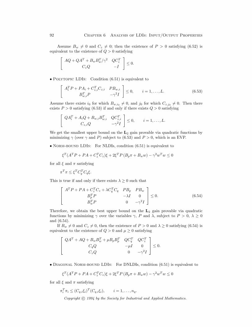
92 Chapter 6 Analysis of LDIs: Input/Output Properties
Assume Bw 6= 0 and Cz 6= 0; then the existence of P > 0 satisfying (6.52) isequivalent to the existence of Q > 0 satisfying
[
AQ+QAT +BwBTw/γ
2 QCTz
CzQ −I
]
≤ 0.
• Polytopic LDIs: Condition (6.51) is equivalent to
[
ATi P + PAi + CT
z,iCz,i PBw,i
BTw,iP −γ2I
]
≤ 0, i = 1, . . . , L. (6.53)
Assume there exists i0 for which Bw,i0 6= 0, and j0 for which Cz,j0 6= 0. Then thereexists P > 0 satisfying (6.53) if and only if there exists Q > 0 satisfying
[
QATi +AiQ+Bw,iB
Tw,i QCT
z,i
Cz,iQ −γ2I
]
≤ 0, i = 1, . . . , L.
We get the smallest upper bound on the L2 gain provable via quadratic functions byminimizing γ (over γ and P ) subject to (6.53) and P > 0, which is an EVP.
• Norm-bound LDIs: For NLDIs, condition (6.51) is equivalent to
ξT (ATP + PA+ CTz Cz)ξ + 2ξTP (Bpπ +Bww)− γ2wTw ≤ 0
for all ξ and π satisfying
πTπ ≤ ξTCTq Cqξ.
This is true if and only if there exists λ ≥ 0 such that
ATP + PA+ CTz Cz + λCT
q Cq PBp PBw
BTp P −λI 0
BTwP 0 −γ2I
≤ 0. (6.54)
Therefore, we obtain the best upper bound on the L2 gain provable via quadraticfunctions by minimizing γ over the variables γ, P and λ, subject to P > 0, λ ≥ 0and (6.54).
If Bw 6= 0 and Cz 6= 0, then the existence of P > 0 and λ ≥ 0 satisfying (6.54) isequivalent to the existence of Q > 0 and µ ≥ 0 satisfying
QAT +AQ+BwBTw + µBpB
Tp QCT
q QCTz
CqQ −µI 0
CzQ 0 −γ2I
≤ 0.
• Diagonal Norm-bound LDIs: For DNLDIs, condition (6.51) is equivalent to
ξT (ATP + PA+ CTz Cz)ξ + 2ξTP (Bpπ +Bww)− γ2wTw ≤ 0
for all ξ and π satisfying
πTi πi ≤ (Cq,iξi)T (Cq,iξi), i = 1, . . . , nq.
Copyright c© 1994 by the Society for Industrial and Applied Mathematics.
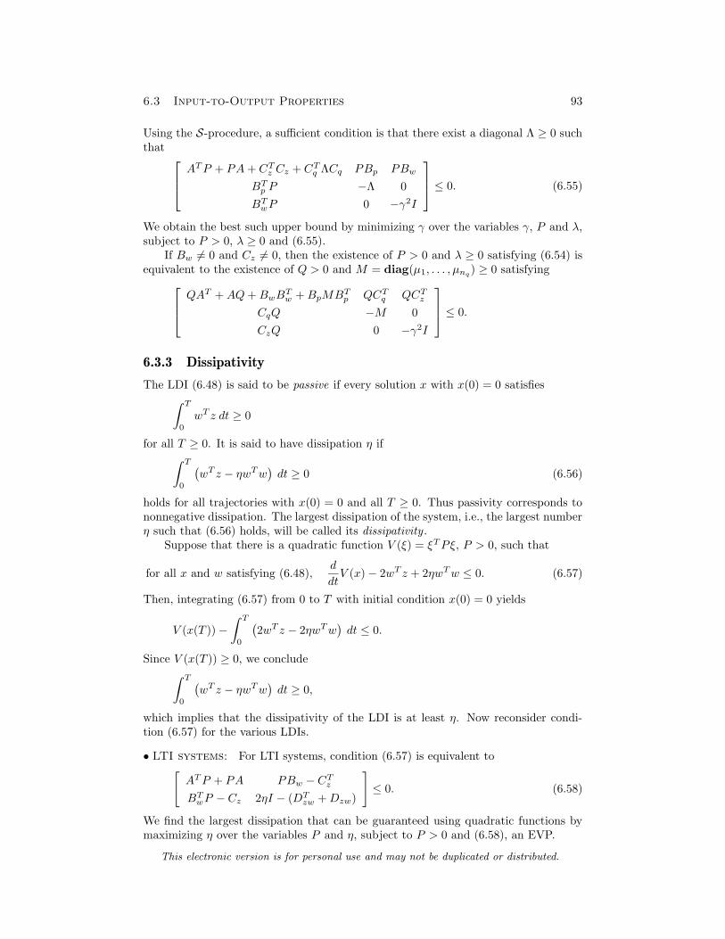
6.3 Input-to-Output Properties 93
Using the S-procedure, a sufficient condition is that there exist a diagonal Λ ≥ 0 suchthat
ATP + PA+ CTz Cz + CT
q ΛCq PBp PBw
BTp P −Λ 0
BTwP 0 −γ2I
≤ 0. (6.55)
We obtain the best such upper bound by minimizing γ over the variables γ, P and λ,subject to P > 0, λ ≥ 0 and (6.55).
If Bw 6= 0 and Cz 6= 0, then the existence of P > 0 and λ ≥ 0 satisfying (6.54) isequivalent to the existence of Q > 0 and M = diag(µ1, . . . , µnq
) ≥ 0 satisfying
QAT +AQ+BwBTw +BpMBT
p QCTq QCT
z
CqQ −M 0
CzQ 0 −γ2I
≤ 0.
6.3.3 Dissipativity
The LDI (6.48) is said to be passive if every solution x with x(0) = 0 satisfies∫ T
0
wT z dt ≥ 0
for all T ≥ 0. It is said to have dissipation η if∫ T
0
(
wT z − ηwTw)
dt ≥ 0 (6.56)
holds for all trajectories with x(0) = 0 and all T ≥ 0. Thus passivity corresponds tononnegative dissipation. The largest dissipation of the system, i.e., the largest numberη such that (6.56) holds, will be called its dissipativity .
Suppose that there is a quadratic function V (ξ) = ξTPξ, P > 0, such that
for all x and w satisfying (6.48),d
dtV (x)− 2wT z + 2ηwTw ≤ 0. (6.57)
Then, integrating (6.57) from 0 to T with initial condition x(0) = 0 yields
V (x(T ))−∫ T
0
(
2wT z − 2ηwTw)
dt ≤ 0.
Since V (x(T )) ≥ 0, we conclude∫ T
0
(
wT z − ηwTw)
dt ≥ 0,
which implies that the dissipativity of the LDI is at least η. Now reconsider condi-tion (6.57) for the various LDIs.
• LTI systems: For LTI systems, condition (6.57) is equivalent to[
ATP + PA PBw − CTz
BTwP − Cz 2ηI − (DT
zw +Dzw)
]
≤ 0. (6.58)
We find the largest dissipation that can be guaranteed using quadratic functions bymaximizing η over the variables P and η, subject to P > 0 and (6.58), an EVP.
This electronic version is for personal use and may not be duplicated or distributed.
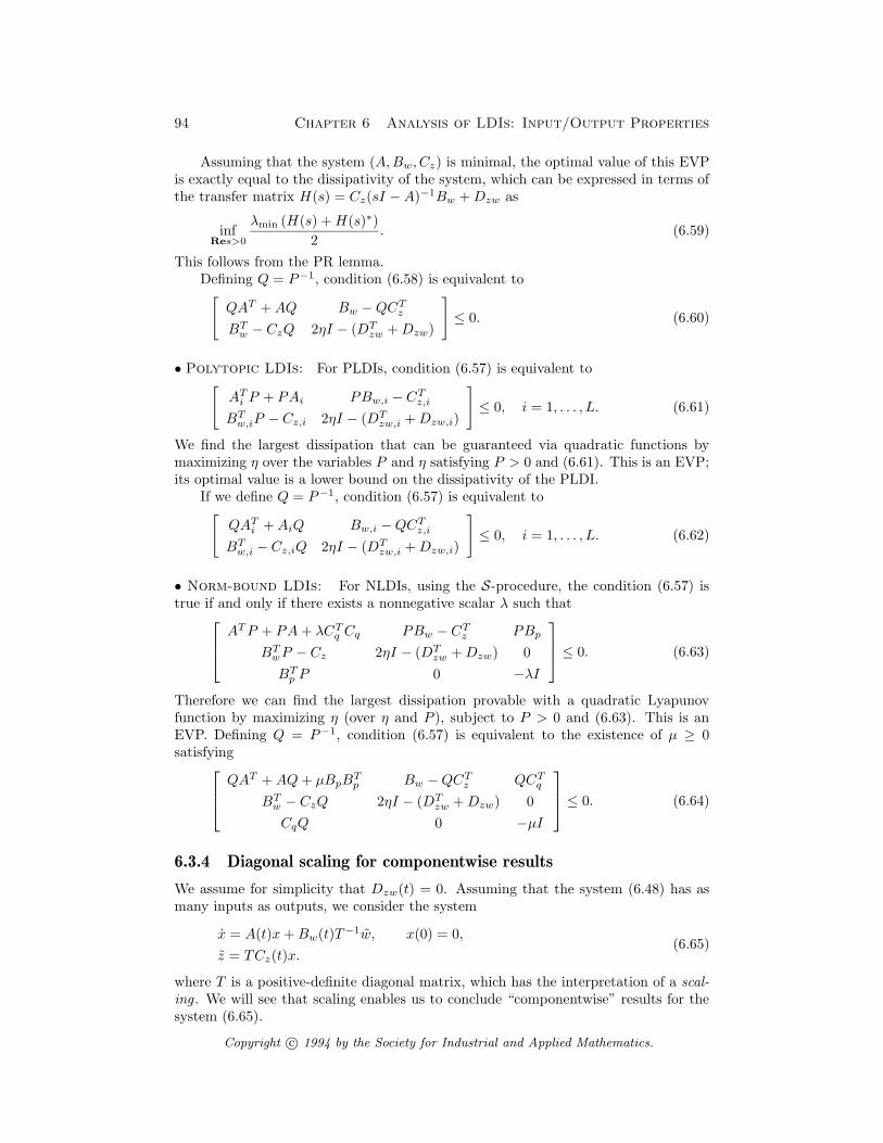
94 Chapter 6 Analysis of LDIs: Input/Output Properties
Assuming that the system (A,Bw, Cz) is minimal, the optimal value of this EVPis exactly equal to the dissipativity of the system, which can be expressed in terms ofthe transfer matrix H(s) = Cz(sI −A)−1Bw +Dzw as
infRes>0
λmin (H(s) +H(s)∗)
2. (6.59)
This follows from the PR lemma.Defining Q = P−1, condition (6.58) is equivalent to[
QAT +AQ Bw −QCTz
BTw − CzQ 2ηI − (DT
zw +Dzw)
]
≤ 0. (6.60)
• Polytopic LDIs: For PLDIs, condition (6.57) is equivalent to[
ATi P + PAi PBw,i − CT
z,i
BTw,iP − Cz,i 2ηI − (DT
zw,i +Dzw,i)
]
≤ 0, i = 1, . . . , L. (6.61)
We find the largest dissipation that can be guaranteed via quadratic functions bymaximizing η over the variables P and η satisfying P > 0 and (6.61). This is an EVP;its optimal value is a lower bound on the dissipativity of the PLDI.
If we define Q = P−1, condition (6.57) is equivalent to[
QATi +AiQ Bw,i −QCT
z,i
BTw,i − Cz,iQ 2ηI − (DT
zw,i +Dzw,i)
]
≤ 0, i = 1, . . . , L. (6.62)
• Norm-bound LDIs: For NLDIs, using the S-procedure, the condition (6.57) istrue if and only if there exists a nonnegative scalar λ such that
ATP + PA+ λCTq Cq PBw − CT
z PBp
BTwP − Cz 2ηI − (DT
zw +Dzw) 0
BTp P 0 −λI
≤ 0. (6.63)
Therefore we can find the largest dissipation provable with a quadratic Lyapunovfunction by maximizing η (over η and P ), subject to P > 0 and (6.63). This is anEVP. Defining Q = P−1, condition (6.57) is equivalent to the existence of µ ≥ 0satisfying
QAT +AQ+ µBpBTp Bw −QCT
z QCTq
BTw − CzQ 2ηI − (DT
zw +Dzw) 0
CqQ 0 −µI
≤ 0. (6.64)
6.3.4 Diagonal scaling for componentwise results
We assume for simplicity that Dzw(t) = 0. Assuming that the system (6.48) has asmany inputs as outputs, we consider the system
x = A(t)x+Bw(t)T−1w, x(0) = 0,
z = TCz(t)x.(6.65)
where T is a positive-definite diagonal matrix, which has the interpretation of a scal-
ing . We will see that scaling enables us to conclude “componentwise” results for thesystem (6.65).
Copyright c© 1994 by the Society for Industrial and Applied Mathematics.
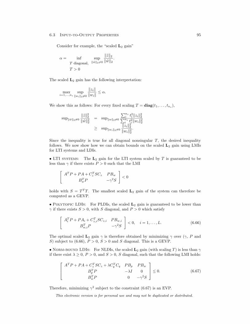
6.3 Input-to-Output Properties 95
Consider for example, the “scaled L2 gain”
α = infT diagonal,
T > 0
sup‖w‖2 6=0
‖z‖2‖w‖2
.
The scaled L2 gain has the following interpretation:
maxi=1,...,nz
sup‖wi‖2 6=0
‖zi‖‖wi‖
≤ α.
We show this as follows: For every fixed scaling T = diag(t1, . . . , tnz),
sup‖w‖2 6=0‖z‖22‖w‖22
= sup‖w‖2 6=0
∑nz
i t2i ‖zi‖22∑nz
i t2i ‖wi‖22≥ sup‖wi‖2 6=0
‖zi‖22‖wi‖22
.
Since the inequality is true for all diagonal nonsingular T , the desired inequalityfollows. We now show how we can obtain bounds on the scaled L2 gain using LMIsfor LTI systems and LDIs.
• LTI systems: The L2 gain for the LTI system scaled by T is guaranteed to beless than γ if there exists P > 0 such that the LMI
[
ATP + PA+ CTz SCz PBw
BTwP −γ2S
]
< 0
holds with S = T TT . The smallest scaled L2 gain of the system can therefore becomputed as a GEVP.
• Polytopic LDIs: For PLDIs, the scaled L2 gain is guaranteed to be lower thanγ if there exists S > 0, with S diagonal, and P > 0 which satisfy
[
ATi P + PAi + CT
z,iSCz,i PBw,i
BTw,iP −γ2S
]
< 0, i = 1, . . . , L. (6.66)
The optimal scaled L2 gain γ is therefore obtained by minimizing γ over (γ, P andS) subject to (6.66), P > 0, S > 0 and S diagonal. This is a GEVP.
• Norm-bound LDIs: For NLDIs, the scaled L2 gain (with scaling T ) is less than γif there exist λ ≥ 0, P > 0, and S > 0, S diagonal, such that the following LMI holds:
ATP + PA+ CTz SCz + λCT
q Cq PBp PBw
BTp P −λI 0
BTwP 0 −γ2S
≤ 0. (6.67)
Therefore, minimizing γ2 subject to the constraint (6.67) is an EVP.
This electronic version is for personal use and may not be duplicated or distributed.
96 Chapter 6 Analysis of LDIs: Input/Output Properties
Notes and References
Integral quadratic constraints
In §8.2 (and §10.9) we consider a generalization of the NLDI in which the pointwise conditionpT p ≤ qT q is replaced by the integral constraint
∫ ∞
0
pT p dt ≤∫ ∞
0
qT q dt.
Many of the results derived for NLDIs and DNLDIs then become necessary and sufficient.Integral quadratic constraints were introduced by Yakubovich. For a general study of these,we refer the reader to the articles of Yakubovich (see [Yak92] and references therein), andalso Megretsky [Meg93, Meg92a, Meg92b].
Reachable sets for componentwise unit-energy inputs
We study in greater detail the set of states reachable with componentwise unit-energy inputsfor LTI systems (see §6.1.2). We begin by observing that a point x0 belongs to the reachableset if and only if the optimal value of the problem
minimize maxi
∫ ∞
0
w2i dt
subject to x = −Ax+Bww, x(0) = x0, limt→∞
x(t) = 0
is less than one. This is a multi-criterion convex quadratic problem, considered in §10.8. Inthis case, the problem reduces to checking whether the LMI
xT0 Px0 < 1,
[
ATP + PA PB
BTP −R
]
≤ 0,
P > 0, R > 0, diagonal, TrR = 1
is feasible. This shows that the reachable set is the intersection of ellipsoids
ξ | ξTPξ ≤ 1
satisfying equation (6.14).
A variation of this problem is considered in [SZ92], where the authors consider inputs wsatisfying
∫∞
0wwT dt ≤ Q, or equivalently
∫ ∞
0
wTWw dt ≤ TrWQ for every W ≥ 0.
They get necessary conditions characterizing the corresponding reachable set. We now deriveLMI conditions that are both necessary and sufficient.
As before, x0 belongs to the reachable set if and only the optimal value of the problem
minimize
∫ ∞
0
wTWw dt
subject to x = −Ax+Bww, x(0) = x0, limt→∞
x(t) = 0
is less than TrWQ for every W ≥ 0. This is equivalent to infeasibility of the LMI (in thevariables P and W ):
xT0 Px0 −TrWQ ≥ 0, P > 0,
[
ATP + PA PB
BTP −W
]
≤ 0.
Copyright c© 1994 by the Society for Industrial and Applied Mathematics.
Notes and References 97
These are precisely the conditions obtained in [SZ92].
Reachable sets with unit-peak inputs
Schweppe [Sch73, §4.3.3] considers the more general problem of time-varying ellipsoidal ap-proximations of reachable sets with unit-peak inputs for time-varying systems; the positive-definite matrix describing the ellipsoidal approximation satisfies a matrix differential equa-tion, terms of which closely resemble those in the matrix inequalities described in this book.Sabin and Summers [SS90] study the approximation of the reachable set via quadratic func-tions. A survey of the available techniques can be found in the article by Gayek [Gay91].See also [FG88].
The technique used to derive LMI (6.23) can be interpreted as an exponential time-weightingprocedure. Fix α > 0. Then for every T > 0, rewrite LDI (6.1), with new exponentially
time-weighted variables xT (t) = eα(t−T )/2x(t) and v(t) = eα(t−T )/2w(t) as
xT =(
A(t) +α
2I)
xT +Bw(t)v, xT (0) = 0.
Since w(t)Tw(t) ≤ 1, we have∫ T
0vT v dτ ≤ 1/α.
Now suppose that P > 0 satisfies condition (6.23), which we rewrite for convenience as
[
(A+ αI/2)TP + P (A+ αI/2) PBw
BTwP −αI
]
≤ 0. (6.68)
The results of §6.1.1 imply that xT (T ) satisfies xT (T )TPxT (T ) ≤ 1; therefore, x(T )TPx(T ) ≤
1. Since LMI (6.68) is independent of T , the ellipsoid
x | xTPx ≤ 1
contains the reachableset with unit-peak inputs.
Bounds on overshoot
The results of §6.1.3 can be used to find a bound on the step response peak for LDIs. Considera single-input single-output LDI, subject to a unit-step input:
x = A(t)x+ bw(t), x(0) = 0,
s = cz(t)x,
[
A(t) bw(t)
cz(t) 0
]
∈ Ω.
Since a unit-step is also a unit-peak input, an upper bound on maxt≥0 |s(t)| (i.e., the over-shoot) can be found by combining the results on reachable sets with unit-peak inputs (§6.1.3)and bounds on output peak (§6.2.2).Suppose there exist Q > 0 and α > 0 satisfying (6.25),
A(t)Q+QA(t)T + αQ+1
αbw(t)bw(t)
T < 0.
Then, from §6.2.2, we conclude that maxt≥0 |s(t)| does not exceed M , where M2 = maxt≥0cz(t)
TQcz(t). This can be used to find LMI-based bounds on overshoot for LTI systems,PLDIs and NLDIs. We note that the resulting bounds can be quite conservative. TheseLMIs can be used to determine state-feedback matrices as well (see the Notes and Referencesof Chapter 7).
This electronic version is for personal use and may not be duplicated or distributed.
98 Chapter 6 Analysis of LDIs: Input/Output Properties
Bounds on impulse response peak for LTI systems
The impulse response h(t) = ceAtb of the single-input single-output LTI system
x = Ax+ bu, x(0) = 0, y = cx
is just the output y with initial condition x(0) = b and zero input. Therefore, we can com-pute a bound on the impulse response peak by combining the results on invariant ellipsoidsfrom §5.2 with those on the peak value of the output from §6.2.2. The bound obtained thisway can be quite conservative. For instance, consider the LTI system with transfer function
H(s) =1
s+ s1
n∏
i=2
s− sis+ si
,
where si+1 À si > 0, i.e., the dynamics of this system are widely spaced. The bound onthe peak value of the impulse response of the system computed via the EVP (6.47) turnsout to be 2n − 1 times the actual maximum value of the impulse response, where n is thedimension of a minimal realization of the system [Fer93]. We conjecture that the boundcan be no more conservative, that is, for every LTI system, the bound on the peak of theimpulse response computed via the EVP (6.47) can be no more than 2n− 1 times the actualmaximum value of the impulse response.
Examples for which the bound obtained via the EVP (6.47) is sharp include the case of passiveLTI systems. In this case, we know there exists a positive-definite P such that ATP+PA ≤ 0,Pb = cT , so that the maximum value of the impulse response is cb and is attained for t = 0.This is an illustration of the fact that passive systems have nice “peaking” properties, whichis used in nonlinear control [Kok92].
Copyright c© 1994 by the Society for Industrial and Applied Mathematics.

Chapter 7
State-Feedback Synthesis for LDIs
7.1 Static State-Feedback Controllers
We consider the LDI
x = A(t)x+Bw(t)w +Bu(t)u, z = Cz(t)x+Dzw(t)w +Dzu(t)u,
[
A(t) Bw(t) Bu(t)
Cz(t) Dzw(t) Dzu(t)
]
∈ Ω,
(7.1)
where Ω has one of our special forms (i.e., singleton, polytope, image of a unit ballunder a matrix linear-fractional mapping). Here u : R+ → Rnu is the control input
and w : R+ → Rnw is the exogenous input signal .Let K ∈ Rnu×n, and suppose that u = Kx. Since the control input is a linear
function of the state, this is called (linear, constant) state-feedback , and the matrix Kis called the state-feedback gain. This yields the closed-loop LDI
x = (A(t) +Bu(t)K)x+Bw(t)w,
z = (Cz(t) +Dzu(t)K)x+Dzw(t)w.(7.2)
In this chapter we consider the state-feedback synthesis problem, i.e., the problem offinding a matrix K so that the closed-loop LDI (7.2) satisfies certain properties orspecifications, e.g., stability.
Remark: Using the idea of global linearization described in §4.3, the methods ofthis chapter can be used to synthesize a linear state-feedback for some nonlinear,time-varying systems. As an example, we can synthesize a state-feedback for thesystem
x = f(x,w, u, t), z = g(x,w, u, t),
provided we have
∂f
∂x
∂f
∂w
∂f
∂u
∂g
∂x
∂g
∂w
∂g
∂u
(x,w, u, t) ∈ Ω,
and f(0, 0, 0, t) = 0, g(0, 0, 0, t) = 0, for all x, t, w and u.
99
100 Chapter 7 State-Feedback Synthesis for LDIs
7.2 State Properties
We consider the LDI
x = A(t)x+Bu(t)u, [A(t) Bu(t)] ∈ Ω. (7.3)
• LTI systems: For LTI systems, (7.3) becomes
x = Ax+Buu. (7.4)
• Polytopic LDIs: PLDIs are given by
x = A(t)x+Bu(t)u, [A(t) Bu(t)] ∈ Co [A1 Bu,1] , . . . . [AL Bu,L] . (7.5)
• Norm-bound LDIs: For NLDIs, (7.3) becomes
x = Ax+Buu+Bpp, q = Cqx+Dquu+Dqpp
p = ∆(t)q, ‖∆(t)‖ ≤ 1.(7.6)
Equivalently, we have
x = Ax+Buu+Bpp, q = Cqx+Dqpp+Dquu, pT p ≤ qT q.
• Diagonal Norm-bound LDIs: For DNLDIs, equation (7.3) becomes
x = Ax+Buu+Bpp, q = Cqx+Dqpp+Dquu,
pi = δi(t)qi, |δi(t)| ≤ 1, i = 1, . . . , L.(7.7)
Equivalently, we have
x = Ax+Buu+Bpp, q = Cqx+Dqpp+Dquu,
|pi| ≤ |qi|, i = 1, . . . , nq.
7.2.1 Quadratic stabilizability
The system (7.1) is said to be quadratically stabilizable (via linear state-feedback) ifthere exists a state-feedback gain K such that the closed-loop system (7.2) is quadrat-ically stable (hence, stable). Quadratic stabilizability can be expressed as an LMIP.
• LTI systems: Let us fix the matrix K. The LTI system (7.4) is (quadratically)stable if and only if there exists P > 0 such that
(A+BuK)TP + P (A+BuK) < 0,
or equivalently, there exists Q > 0 such that
Q(A+BuK)T + (A+BuK)Q < 0. (7.8)
Neither of these conditions is jointly convex in K and P or Q, but by a simple changeof variables we can obtain an equivalent condition that is an LMI.
Define Y = KQ, so that for Q > 0 we have K = Y Q−1. Substituting into (7.8)yields
AQ+QAT +BuY + Y TBTu < 0, (7.9)
Copyright c© 1994 by the Society for Industrial and Applied Mathematics.
7.2 State Properties 101
which is an LMI in Q and Y . Thus, the system (7.4) is quadratically stabilizable ifand only if there exist Q > 0 and Y such that the LMI (7.9) holds. If this LMI isfeasible, then the quadratic function V (ξ) = ξTQ−1ξ proves (quadratic) stability ofsystem (7.4) with state-feedback u = Y Q−1x.
Remark: We will use the simple change of variables Y = KQ many times inthe sequel. It allows us to recast the problem of finding a state-feedback gainas an LMIP with variables that include Q and Y ; the state-feedback gain K isrecovered as K = Y Q−1.
An alternate equivalent condition for (quadratic) stabilizability, involving fewervariables, can be derived using the elimination of matrix variables described in §2.6.2:There exist Q > 0 and a scalar σ such that
AQ+QAT − σBuBTu < 0. (7.10)
Since we can always assume σ > 0 in LMI (7.10), and since the LMI is homogeneousin Q and σ, we can without loss of generality take σ = 1, thus reducing the number ofvariables by one. If Q > 0 satisfies the LMI (7.10), a stabilizing state-feedback gain isgiven by K = −(σ/2)BT
uQ−1.
From the elimination procedure of §2.6.2, another equivalent condition is
BTu
(
AQ+QAT)
Bu < 0, (7.11)
where Bu is an orthogonal complement of Bu. For any Q > 0 satisfying (7.11), astabilizing state-feedback gain is K = −(σ/2)BT
uQ−1, where σ is any scalar such
that (7.10) holds (condition (7.11) implies that such a scalar exists).For LTI systems, these LMI conditions are necessary and sufficient for stabiliz-
ability. In terms of linear system theory, stabilizability is equivalent to the conditionthat every unstable mode be controllable; it is not hard to show that this is equivalentto feasibility of the LMIs (7.9), (7.11), or (7.10).
• Polytopic LDIs: For the PLDI (7.5), the same argument applies. Quadraticstabilizability is equivalent to the existence of Q > 0 and Y with
QATi +AiQ+Bu,iY + Y TBT
u,i < 0, i = 1, . . . , L. (7.12)
• Norm-bound LDIs: With u = Kx, the NLDI (7.6) is quadratically stable (seeLMI (5.14)) if there exist Q > 0 and µ > 0 such that
(
AQ+QAT +BuKQ
+QKTBTu + µBpB
Tp
)
µBpDTqp +Q(Cq +DquK)T
µDqpBTp + (Cq +DquK)Q −µ(I −DqpD
Tqp)
< 0.
This condition has a simple frequency-domain interpretation: The H∞ norm of thetransfer matrix from p to q for the LTI system x = (A + BuK)x + Bpp, q = (Cq +DquK)x+Dqpp is less than one.
With Y = KQ, we conclude that the NLDI is quadratically stabilizable if thereexist Q > 0, µ > 0 and Y such that
(
AQ+QAT + µBpBTp
+BuY + Y TBTu
)
µBpDTqp +QCT
q + Y TDTqu
µDqpBTp + CqQ+DquY − µ(I −DqpD
Tqp)
< 0. (7.13)
This electronic version is for personal use and may not be duplicated or distributed.
102 Chapter 7 State-Feedback Synthesis for LDIs
Using the elimination procedure of §2.6.2, we obtain the equivalent conditions:
(
AQ+QAT
− σBuBTu + µBpB
Tp
)
QCTq + µBpD
Tqp − σBuD
Tqu
CqQ+ µDqpBTp − σDquB
Tu −µ(I −DqpD
Tqp)− σDquD
Tqu
< 0,
−µ(I −DqpDTqp) < 0.
(7.14)
The latter condition is always satisfied since the NLDI is well-posed. By homogeneity,we can set µ = 1. If Q > 0 and σ > 0 satisfy (7.14) with µ = 1, a stabilizingstate-feedback gain is K = (−σ/2)BT
uQ−1.
An alternate, equivalent condition for quadratic stabilizability is expressed interms of the orthogonal complement of [BT
u DTqu]
T , which we denote by G:
GT
[
AQ+QAT + µBpBTp QCT
q + µBpDTqp
CqQ+ µDqpBTp −µ(I −DqpD
Tqp)
]
G < 0. (7.15)
(Again, we can freely set µ = 1 in this LMI.)In the remainder of this chapter we will assume that Dqp in (7.6) is zero in order
to simplify the discussion; all the following results can be extended to the case inwhich Dqp is nonzero.
• Diagonal Norm-bound LDIs: With u = Kx, the DNLDI (7.7) is quadraticallystable (see LMI (5.16)) if there exist Q > 0, M = diag(µ1, . . . , µnq
) > 0 satisfying
(
AQ+QAT +BuKQ
+QKTBTu +BpMBT
p
)
BpMDTqp +Q(Cq +DquK)T
DqpMBTp + (Cq +DquK)Q −(M −DqpMDT
qp)
< 0.
This condition leads to a simple frequency-domain interpretation for quadratic stabi-lizability of DNLDIs: Let H denote the transfer matrix from p to q for the LTI systemx = (A+BuK)x+Bpp, q = (Cq +DquK)x+Dqpp. Then the DNLDI is quadraticallystabilizable if there exists K such that for some diagonal positive-definite matrix M ,‖M−1/2HM1/2‖∞ ≤ 1. There is no analytical method for checking this condition.
With Y = KQ, we conclude that the NLDI is quadratically stabilizable if thereexist Q > 0, M > 0 and diagonal, and Y such that
(
AQ+QAT +BpMBTp
+BuY + Y TBTu
)
BpMDTqp +QCT
q + Y TDTqu
DqpMBTp + CqQ+DquY − (M −DqpMDT
qp)
< 0.
As before, we can eliminate the variable Y using the elimination procedure of §2.6.2,and obtain equivalent LMIs in fewer variables.
7.2.2 Holdable ellipsoids
Just as quadratic stability can also be interpreted in terms of invariant ellipsoids, wecan interpret quadratic stabilizability in terms of holdable ellipsoids. We say that theellipsoid
E =
ξ ∈ Rn∣
∣ ξTQ−1ξ ≤ 1
Copyright c© 1994 by the Society for Industrial and Applied Mathematics.

7.2 State Properties 103
is holdable for the system (7.3) if there exists a state-feedback gain K such that Eis invariant for the system (7.3) with u = Kx. Therefore the LMIs described in theprevious section also characterize holdable ellipsoids for the system (7.3).
With this parametrization of quadratic stabilizability and holdable ellipsoids asLMIs in Q > 0 and Y , we can solve various optimization problems, such as findingthe coordinate transformation that minimizes the condition number of Q, imposingnorm constraints on the input u = Kx, etc.
Remark: In Chapter 5, we saw that quadratic stability and invariant ellipsoidswere characterized by LMIs in a variable P > 0 and also its inverse Q = P−1.In contrast, quadratic stabilizability and ellipsoid holdability can be expressedas LMIs only in variables Q and Y ; it is not possible to rewrite these LMIs asLMIs with Q−1 as a variable. This restricts the extension of some of the resultsfrom Chapter 5 (and Chapter 6) to state-feedback synthesis. As a rule of thumb,results in the analysis of LDIs that are expressed as LMIs in the variable Q canbe extended to state-feedback synthesis, with a few exceptions; results expressedas LMIs in P are not. For example, we will not be able to compute the minimumvolume holdable ellipsoid that contains a given polytope P (see problem (5.33))as an optimization problem over LMIs; however, we will be able to compute theminimum diameter holdable ellipsoid (see problem (5.34)) containing P.
7.2.3 Constraints on the control input
When the initial condition is known, we can find an upper bound on the norm ofthe control input u(t) = Kx(t) as follows. Pick Q > 0 and Y which satisfy thequadratic stabilizability condition (either (7.9), (7.12) or (7.13)), and in additionx(0)TQ−1x(0) ≤ 1. This implies that x(t) belongs to E for all t ≥ 0, and conse-quently,
maxt≥0
‖u(t)‖ = maxt≥0 ‖Y Q−1x(t)‖≤ maxx∈E ‖Y Q−1x‖= λmax(Q
−1/2Y TY Q−1/2).
Therefore, the constraint ‖u(t)‖ ≤ µ is enforced at all times t ≥ 0 if the LMIs
[
1 x(0)T
x(0) Q
]
≥ 0,
[
Q Y T
Y µ2I
]
≥ 0 (7.16)
hold, where Q > 0 and Y satisfy the stabilizability conditions (either (7.9), (7.12)or (7.13)).
We can extend this to the case where x(0) lies in an ellipsoid or polytope. Forexample suppose we require (7.16) to hold for all ‖x(0‖ ≤ 1. This is easily shown tobe equivalent to
Q ≥ I,
[
Q Y T
Y µ2I
]
≥ 0.
As another extension we can handle constraints on
‖u(t)‖max ∆= maxi|ui(t)|
This electronic version is for personal use and may not be duplicated or distributed.

104 Chapter 7 State-Feedback Synthesis for LDIs
in a similar manner:
maxt≥0
‖u(t)‖max = maxt≥0 ‖Y Q−1x(t)‖max≤ maxx∈E ‖Y Q−1x‖max= maxi
(
Y Q−1Y T)
ii.
Therefore, the constraint ‖u(t)‖max ≤ µ for t ≥ 0 is implied by the LMI[
1 x(0)T
x(0) Q
]
≥ 0,
[
X Y
Y T Q
]
≥ 0, Xii ≤ µ2,
where once again, Q > 0 and Y satisfy the stabilizability conditions (either (7.9),(7.12) or (7.13)).
7.3 Input-to-State Properties
We next consider the LDI
x = A(t)x+Bw(t)w +Bu(t)u. (7.17)
• LTI systems: For LTI systems, equation (7.17) becomes x = Ax+Bww +Buu.
• Polytopic LDIs: PLDIs are given by x = A(t)x + Bw(t)w + Bu(t)u, where[A(t) Bw(t) Bu(t)] ∈ Co [A1 Bw,1 Bu,1] , . . . , [AL Bw,L Bu,L].
• Norm-bound LDIs: For NLDIs, equation (7.17) becomes
x = Ax+Buu+Bpp+Bww, q = Cqx+Dquu
p = ∆(t)q, ‖∆(t)‖ ≤ 1
which we can also express as
x = Ax+Buu+Bpp+Bww, q = Cqx+Dquu, pT p ≤ qT q.
• Diagonal Norm-bound LDIs: For DNLDIs, equation (7.17) becomes
x = Ax+Buu+Bpp+Bww, q = Cqx+Dquu
pi = δi(t)qi, |δi(t)| ≤ 1, i = 1, . . . , L.
Equivalently, we have
x = Ax+Buu+Bpp+Bww, q = Cqx+Dquu,
|pi| ≤ |qi|, i = 1, . . . , nq.
7.3.1 Reachable sets with unit-energy inputs
For the system (7.17) with u = Kx, the set of states reachable with unit energy isdefined as
Rue ∆=
x(T )
∣
∣
∣
∣
∣
∣
∣
x, w, u satisfy (7.17), u = Kx, x(0) = 0,∫ T
0
wTw dt ≤ 1, T ≥ 0
.
Copyright c© 1994 by the Society for Industrial and Applied Mathematics.
7.3 Input-to-State Properties 105
We will now derive conditions under which there exists a state-feedback gain K guar-anteeing that a given ellipsoid E = ξ ∈ Rn
∣
∣ ξTQ−1ξ ≤ 1 contains Rue.
• LTI systems: From §6.1.1, the ellipsoid E contains Rue for the system (7.4) forsome state-feedback gain K if K satisfies
AQ+QAT +BuKQ+QKTBTu +BwB
Tw ≤ 0.
Setting KQ = Y , we conclude that E ⊇ Rue for some K if there exist Y such that
QAT +AQ+BuY + Y TBTu +BwB
Tw ≤ 0.
For any Q > 0 and Y satisfying this LMI, the state-feedback gain K = Y Q−1 is suchthat the ellipsoid E contains the reachable set for the closed-loop system.
Using the elimination procedure of §2.6.2, we eliminate the variable Y to obtainthe LMI in Q > 0 and the variable σ:
QAT +AQ− σBuBTu +BwB
Tw ≤ 0. (7.18)
For any Q > 0 and σ satisfying this LMI, a corresponding state-feedback gain is givenby K = −(σ/2)BT
uQ−1. Another equivalent condition for E to contain Rue is
BTu
(
AQ+QAT +BwBTw
)
Bu ≤ 0, (7.19)
where Bu is an orthogonal complement of Bu.
• Polytopic LDIs: For PLDIs, E contains Rue for some state-feedback gain K ifthere exist Q > 0 and Y such that the following LMI holds (see LMI (6.9)):
QATi +AiQ+Bu,iY + Y TBT
u,i +Bw,iBTw,i < 0, i = 1, . . . , L.
• Norm-bound LDIs: For NLDIs, E contains Rue for some state-feedback gain Kif there exist µ > 0 and Y such that the following LMI holds (see LMI (6.11)):
[
QAT +AQ+BuY + Y TBTu +BwB
Tw + µBpB
Tp (CqQ+DquY )T
CqQ+DquY −µI
]
≤ 0.
We can eliminate Y to obtain the LMI in Q > 0 and σ that guarantees that E containsthe reachable set Rue for some state-feedback gain K:
(
AQ+QAT − σBuBTu
+µBpBTp +BwB
Tw
)
QCTq + µBpD
Tqp − σBuD
Tqu
CqQ+ µDqpBTp − σDquB
Tu −µ(I −DqpD
Tqp)− σDquD
Tqu
< 0. (7.20)
The corresponding state-feedback gain is K = (−σ/2)BTuQ
−1.An equivalent condition is expressed in terms of G, the orthogonal complement
of [BTu DT
qu]T :
GT
(
AQ+QAT
+µBpBTp +BwB
Tw
)
QCTq + µBpD
Tqp
CqQ+ µDqpBTp −µ(I −DqpD
Tqp)
G < 0.
This electronic version is for personal use and may not be duplicated or distributed.
106 Chapter 7 State-Feedback Synthesis for LDIs
• Diagonal Norm-bound LDIs: For DNLDIs, E contains Rue for some state-feedback gain K if there exist Q > 0, M > 0 and diagonal, and Y such that thefollowing LMI holds (see LMI (6.12)):
[
QAT +AQ+BuY + Y TBTu +BwB
Tw +BpMBT
p (CqQ+DquY )T
CqQ+DquY −M
]
≤ 0.
Using the elimination procedure of §2.6.2, we can eliminate the variable Y to obtainan equivalent LMI in fewer variables.
Using these LMIs (see §6.1.1 for details):
• We can find a state-feedback gain K such that a given point x0 lies outside theset of reachable states for the system (7.3).
• We can find a state-feedback gain K such that the set of reachable states for thesystem (7.3) lies in a given half-space. This result can be extended to check ifthe reachable set is contained in a polytope. In this case, in contrast with theresults in Chapter 6, we must use the same outer ellipsoidal approximation tocheck different faces. (This is due to the coupling induced by the new variableY = KQ.)
7.3.2 Reachable sets with componentwise unit-energy inputs
With u = Kx, the set of reachable states for inputs with componentwise unit-energyfor the system (7.17) is defined as
Ruce ∆=
x(T )
∣
∣
∣
∣
∣
∣
∣
x, w, u satisfy (7.17), u = Kx, x(0) = 0,∫ T
0
wTi wi dt ≤ 1, T ≥ 0
.
We now consider the existence of the state-feedback gain K such that the ellipsoidE = ξ ∈ Rn
∣
∣ ξTQ−1ξ ≤ 1 contains Ruce for LTI systems and LDIs.
• LTI systems: From LMI (6.15), E ⊇ Ruce for the LTI system (7.4) if there existsdiagonal R > 0 with unit trace such that the LMI
[
QAT +AQ+BuY + Y TBTu Bw
BTw −R
]
≤ 0.
• Polytopic LDIs: For PLDIs, E ⊇ Ruce for some state-feedback gain K if thereexist Q > 0, Y (= KQ), and a diagonal R > 0 with unit trace (see LMI (6.17)), suchthat
[
QATi +AiQ+Bu,iY + Y TBT
u,i Bw,i
BTw,i −R
]
< 0, i = 1, . . . , L.
• Norm-bound LDIs: For NLDIs, E ⊇ Ruce for some state-feedback gain K if thereexist Q > 0, µ > 0, Y and a diagonal R > 0 with unit trace (see LMI (6.19)), suchthat
QAT + Y TBTu +AQ+BuY + µBpB
Tp QCT
q + Y TDTqu Bw
CqQ+DquY −µI 0
BTw 0 −R
≤ 0.
Copyright c© 1994 by the Society for Industrial and Applied Mathematics.
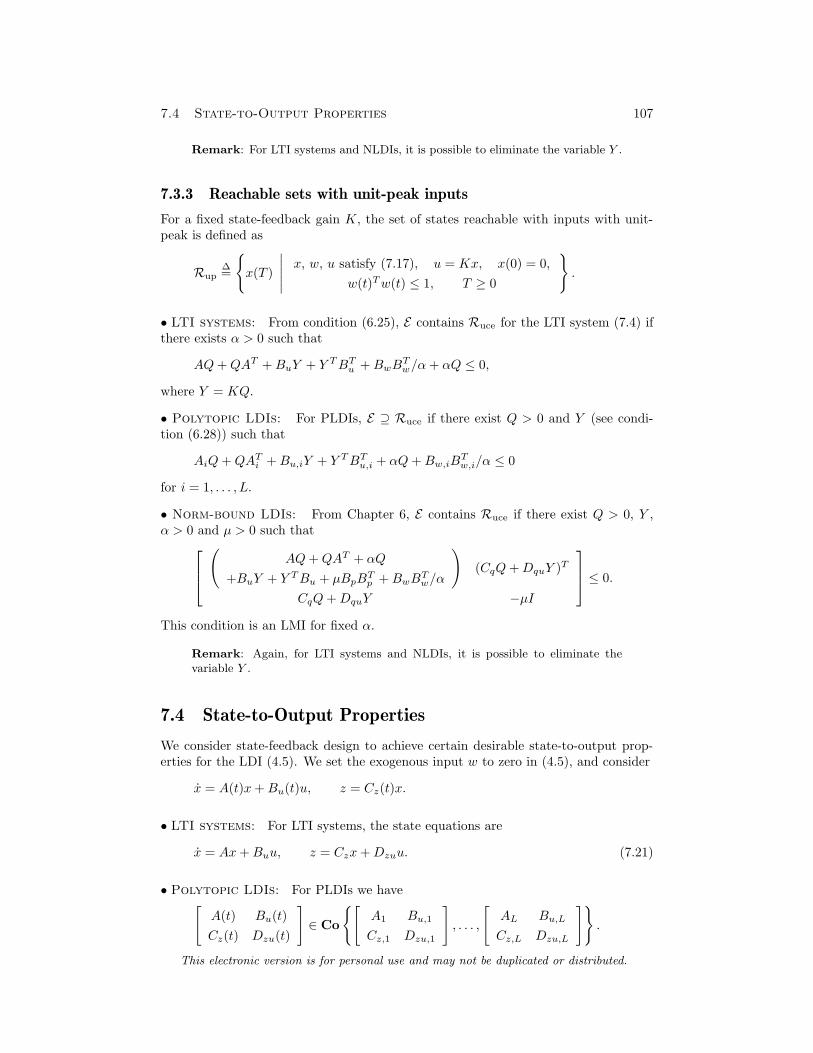
7.4 State-to-Output Properties 107
Remark: For LTI systems and NLDIs, it is possible to eliminate the variable Y .
7.3.3 Reachable sets with unit-peak inputs
For a fixed state-feedback gain K, the set of states reachable with inputs with unit-peak is defined as
Rup ∆=
x(T )
∣
∣
∣
∣
∣
x, w, u satisfy (7.17), u = Kx, x(0) = 0,
w(t)Tw(t) ≤ 1, T ≥ 0
.
• LTI systems: From condition (6.25), E contains Ruce for the LTI system (7.4) ifthere exists α > 0 such that
AQ+QAT +BuY + Y TBTu +BwB
Tw/α+ αQ ≤ 0,
where Y = KQ.
• Polytopic LDIs: For PLDIs, E ⊇ Ruce if there exist Q > 0 and Y (see condi-tion (6.28)) such that
AiQ+QATi +Bu,iY + Y TBT
u,i + αQ+Bw,iBTw,i/α ≤ 0
for i = 1, . . . , L.
• Norm-bound LDIs: From Chapter 6, E contains Ruce if there exist Q > 0, Y ,α > 0 and µ > 0 such that
(
AQ+QAT + αQ
+BuY + Y TBu + µBpBTp +BwB
Tw/α
)
(CqQ+DquY )T
CqQ+DquY −µI
≤ 0.
This condition is an LMI for fixed α.
Remark: Again, for LTI systems and NLDIs, it is possible to eliminate thevariable Y .
7.4 State-to-Output Properties
We consider state-feedback design to achieve certain desirable state-to-output prop-erties for the LDI (4.5). We set the exogenous input w to zero in (4.5), and consider
x = A(t)x+Bu(t)u, z = Cz(t)x.
• LTI systems: For LTI systems, the state equations are
x = Ax+Buu, z = Czx+Dzuu. (7.21)
• Polytopic LDIs: For PLDIs we have[
A(t) Bu(t)
Cz(t) Dzu(t)
]
∈ Co
[
A1 Bu,1
Cz,1 Dzu,1
]
, . . . ,
[
AL Bu,L
Cz,L Dzu,L
]
.
This electronic version is for personal use and may not be duplicated or distributed.
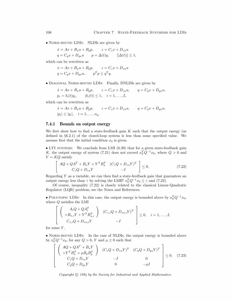
108 Chapter 7 State-Feedback Synthesis for LDIs
• Norm-bound LDIs: NLDIs are given by
x = Ax+Buu+Bpp, z = Czx+Dzuu
q = Cqx+Dquu p = ∆(t)q, ‖∆(t)‖ ≤ 1,
which can be rewritten as
x = Ax+Buu+Bpp, z = Czx+Dzuu
q = Cqx+Dquu, pT p ≤ qT q.
• Diagonal Norm-bound LDIs: Finally, DNLDIs are given by
x = Ax+Buu+Bpp, z = Czx+Dzuu, q = Cqx+Dquu,
pi = δi(t)qi, |δi(t)| ≤ 1, i = 1, . . . , L.
which can be rewritten as
x = Ax+Buu+Bpp, z = Czx+Dzuu, q = Cqx+Dquu,
|pi| ≤ |qi|, i = 1, . . . , nq.
7.4.1 Bounds on output energy
We first show how to find a state-feedback gain K such that the output energy (asdefined in §6.2.1) of the closed-loop system is less than some specified value. Weassume first that the initial condition x0 is given.
• LTI systems: We conclude from LMI (6.39) that for a given state-feedback gainK, the output energy of system (7.21) does not exceed xT0Q
−1x0, where Q > 0 andY = KQ satisfy
[
AQ+QAT +BuY + Y TBTu (CzQ+DzuY )T
CzQ+DzuY −I
]
≤ 0, (7.22)
Regarding Y as a variable, we can then find a state-feedback gain that guarantees anoutput energy less than γ by solving the LMIP xT0Q
−1x0 ≤ γ and (7.22).Of course, inequality (7.22) is closely related to the classical Linear-Quadratic
Regulator (LQR) problem; see the Notes and References.
• Polytopic LDIs: In this case, the output energy is bounded above by xT0Q−1x0,
where Q satisfies the LMI
(
AiQ+QATi
+Bu,iY + Y TBTu,i
)
(Cz,iQ+Dzu,iY )T
Cz,iQ+Dzu,iY −I
≤ 0, i = 1, . . . , L
for some Y .
• Norm-bound LDIs: In the case of NLDIs, the output energy is bounded aboveby xT0Q
−1x0, for any Q > 0, Y and µ ≥ 0 such that
(
AQ+QAT +BuY
+Y TBTu + µBpB
Tp
)
(CzQ+DzuY )T (CqQ+DquY )T
CzQ+DzuY −I 0
CqQ+DquY 0 −µI
≤ 0. (7.23)
Copyright c© 1994 by the Society for Industrial and Applied Mathematics.
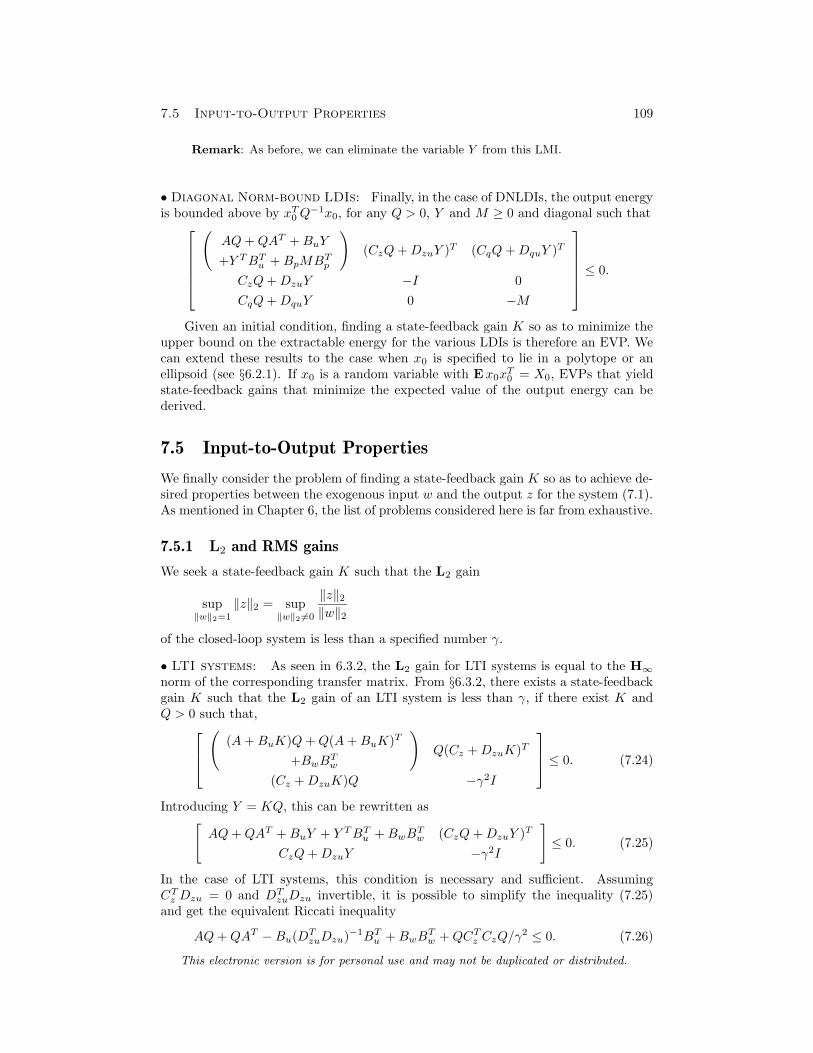
7.5 Input-to-Output Properties 109
Remark: As before, we can eliminate the variable Y from this LMI.
• Diagonal Norm-bound LDIs: Finally, in the case of DNLDIs, the output energyis bounded above by xT0Q
−1x0, for any Q > 0, Y and M ≥ 0 and diagonal such that
(
AQ+QAT +BuY
+Y TBTu +BpMBT
p
)
(CzQ+DzuY )T (CqQ+DquY )T
CzQ+DzuY −I 0
CqQ+DquY 0 −M
≤ 0.
Given an initial condition, finding a state-feedback gain K so as to minimize theupper bound on the extractable energy for the various LDIs is therefore an EVP. Wecan extend these results to the case when x0 is specified to lie in a polytope or anellipsoid (see §6.2.1). If x0 is a random variable with Ex0x
T0 = X0, EVPs that yield
state-feedback gains that minimize the expected value of the output energy can bederived.
7.5 Input-to-Output Properties
We finally consider the problem of finding a state-feedback gain K so as to achieve de-sired properties between the exogenous input w and the output z for the system (7.1).As mentioned in Chapter 6, the list of problems considered here is far from exhaustive.
7.5.1 L2 and RMS gains
We seek a state-feedback gain K such that the L2 gain
sup‖w‖2=1
‖z‖2 = sup‖w‖2 6=0
‖z‖2‖w‖2
of the closed-loop system is less than a specified number γ.
• LTI systems: As seen in 6.3.2, the L2 gain for LTI systems is equal to the H∞
norm of the corresponding transfer matrix. From §6.3.2, there exists a state-feedbackgain K such that the L2 gain of an LTI system is less than γ, if there exist K andQ > 0 such that,
(
(A+BuK)Q+Q(A+BuK)T
+BwBTw
)
Q(Cz +DzuK)T
(Cz +DzuK)Q −γ2I
≤ 0. (7.24)
Introducing Y = KQ, this can be rewritten as[
AQ+QAT +BuY + Y TBTu +BwB
Tw (CzQ+DzuY )T
CzQ+DzuY −γ2I
]
≤ 0. (7.25)
In the case of LTI systems, this condition is necessary and sufficient. AssumingCTz Dzu = 0 and DT
zuDzu invertible, it is possible to simplify the inequality (7.25)and get the equivalent Riccati inequality
AQ+QAT −Bu(DTzuDzu)
−1BTu +BwB
Tw +QCT
z CzQ/γ2 ≤ 0. (7.26)
This electronic version is for personal use and may not be duplicated or distributed.
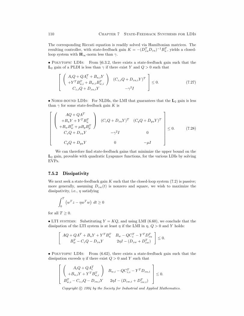
110 Chapter 7 State-Feedback Synthesis for LDIs
The corresponding Riccati equation is readily solved via Hamiltonian matrices. Theresulting controller, with state-feedback gain K = −(DT
zuDzu)−1BT
u , yields a closed-loop system with H∞-norm less than γ.
• Polytopic LDIs: From §6.3.2, there exists a state-feedback gain such that theL2 gain of a PLDI is less than γ if there exist Y and Q > 0 such that
(
AiQ+QATi +Bu,iY
+Y TBTu,i +Bw,iB
Tw,i
)
(Cz,iQ+Dzu,iY )T
Cz,iQ+Dzu,iY −γ2I
≤ 0. (7.27)
• Norm-bound LDIs: For NLDIs, the LMI that guarantees that the L2 gain is lessthan γ for some state-feedback gain K is
AQ+QAT
+BuY + Y TBTu
+BwBTw + µBpB
Tp
(CzQ+DzuY )T (CqQ+DquY )T
CzQ+DzuY −γ2I 0
CqQ+DquY 0 −µI
≤ 0. (7.28)
We can therefore find state-feedback gains that minimize the upper bound on theL2 gain, provable with quadratic Lyapunov functions, for the various LDIs by solvingEVPs.
7.5.2 Dissipativity
We next seek a state-feedback gain K such that the closed-loop system (7.2) is passive;more generally, assuming Dzw(t) is nonzero and square, we wish to maximize thedissipativity, i.e., η satisfying
∫ T
0
(
wT z − ηwTw)
dt ≥ 0
for all T ≥ 0.
• LTI systems: Substituting Y = KQ, and using LMI (6.60), we conclude that thedissipation of the LTI system is at least η if the LMI in η, Q > 0 and Y holds:
[
AQ+QAT +BuY + Y TBTu Bw −QCT
z − Y TDTzu
BTw − CzQ−DzuY 2ηI − (Dzw +DT
zw)
]
≤ 0.
• Polytopic LDIs: From (6.62), there exists a state-feedback gain such that thedissipation exceeds η if there exist Q > 0 and Y such that
(
AiQ+QATi
+Bu,iY + Y TBTu,i
)
Bw,i −QCTz,i − Y TDzu,i
BTw,i − Cz,iQ−Dzu,iY 2ηI − (Dzw,i +DT
zw,i)
≤ 0.
Copyright c© 1994 by the Society for Industrial and Applied Mathematics.
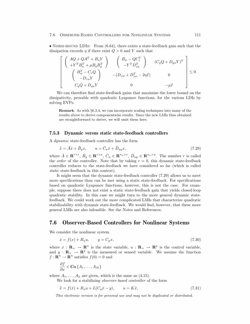
7.6 Observer-Based Controllers for Nonlinear Systems 111
• Norm-bound LDIs: From (6.64), there exists a state-feedback gain such that thedissipation exceeds η if there exist Q > 0 and Y such that
(
AQ+QAT +BuY
+Y TBTu + µBqB
Tq
) (
Bw −QCTz
−Y TDTzu
)
(CqQ+DquY )T
(
BTw − CzQ
−DzuY
)
−(Dzw +DTzw − 2ηI) 0
CqQ+DquY 0 −µI
≤ 0
We can therefore find state-feedback gains that maximize the lower bound on thedissipativity, provable with quadratic Lyapunov functions, for the various LDIs bysolving EVPs.
Remark: As with §6.3.4, we can incorporate scaling techniques into many of theresults above to derive componentwise results. Since the new LMIs thus obtainedare straightforward to derive, we will omit them here.
7.5.3 Dynamic versus static state-feedback controllers
A dynamic state-feedback controller has the form
˙x = Ax+ Byx, u = Cux+ Duyx, (7.29)
where A ∈ Rr×r, By ∈ Rr×n, Cu ∈ Rnu×r, Duy ∈ Rnu×n. The number r is calledthe order of the controller. Note that by taking r = 0, this dynamic state-feedbackcontroller reduces to the state-feedback we have considered so far (which is calledstatic state-feedback in this context).
It might seem that the dynamic state-feedback controller (7.29) allows us to meetmore specifications than can be met using a static state-feedback. For specificationsbased on quadratic Lyapunov functions, however, this is not the case. For exam-ple, suppose there does not exist a static state-feedback gain that yields closed-loopquadratic stability. In this case we might turn to the more general dynamic state-feedback. We could work out the more complicated LMIs that characterize quadraticstabilizability with dynamic state-feedback. We would find, however, that these moregeneral LMIs are also infeasible. See the Notes and References.
7.6 Observer-Based Controllers for Nonlinear Systems
We consider the nonlinear system
x = f(x) +Buu, y = Cyx, (7.30)
where x : R+ → Rn is the state variable, u : R+ → Rp is the control variable,and y : R+ → Rq is the measured or sensed variable. We assume the functionf : Rn → Rn satisfies f(0) = 0 and
∂f
∂x∈ Co A1, . . . , AM
where A1, . . . , AL are given, which is the same as (4.15).We look for a stabilizing observer-based controller of the form
˙x = f(x) +Buu+ L(Cyx− y), u = Kx, (7.31)
This electronic version is for personal use and may not be duplicated or distributed.
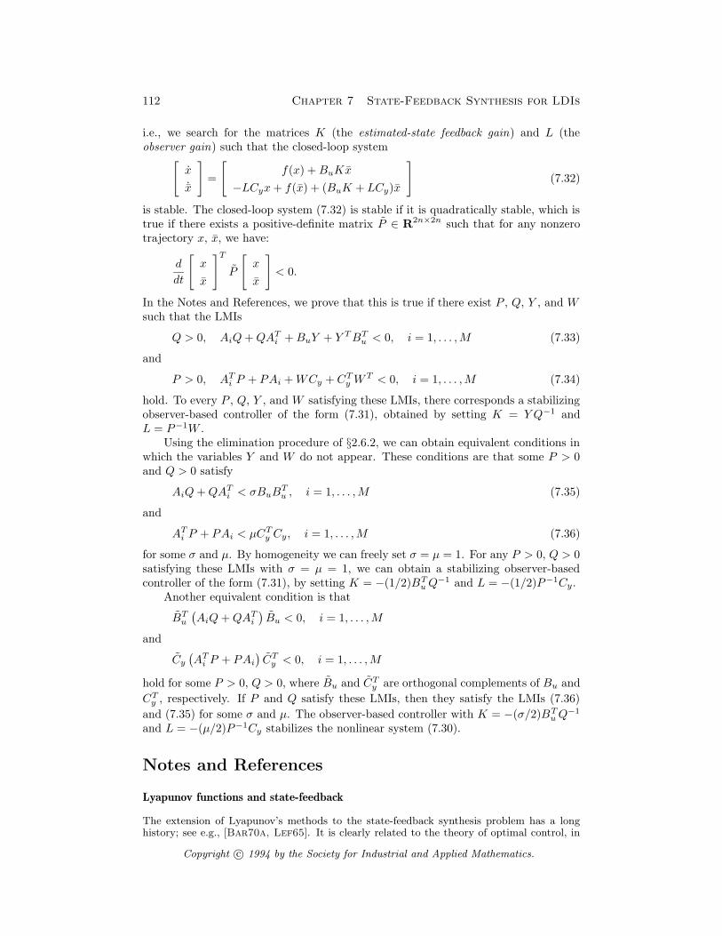
112 Chapter 7 State-Feedback Synthesis for LDIs
i.e., we search for the matrices K (the estimated-state feedback gain) and L (theobserver gain) such that the closed-loop system
[
x
˙x
]
=
[
f(x) +BuKx
−LCyx+ f(x) + (BuK + LCy)x
]
(7.32)
is stable. The closed-loop system (7.32) is stable if it is quadratically stable, which istrue if there exists a positive-definite matrix P ∈ R2n×2n such that for any nonzerotrajectory x, x, we have:
d
dt
[
x
x
]T
P
[
x
x
]
< 0.
In the Notes and References, we prove that this is true if there exist P , Q, Y , and Wsuch that the LMIs
Q > 0, AiQ+QATi +BuY + Y TBT
u < 0, i = 1, . . . ,M (7.33)
and
P > 0, ATi P + PAi +WCy + CT
y WT < 0, i = 1, . . . ,M (7.34)
hold. To every P , Q, Y , and W satisfying these LMIs, there corresponds a stabilizingobserver-based controller of the form (7.31), obtained by setting K = Y Q−1 andL = P−1W .
Using the elimination procedure of §2.6.2, we can obtain equivalent conditions inwhich the variables Y and W do not appear. These conditions are that some P > 0and Q > 0 satisfy
AiQ+QATi < σBuB
Tu , i = 1, . . . ,M (7.35)
and
ATi P + PAi < µCT
y Cy, i = 1, . . . ,M (7.36)
for some σ and µ. By homogeneity we can freely set σ = µ = 1. For any P > 0, Q > 0satisfying these LMIs with σ = µ = 1, we can obtain a stabilizing observer-basedcontroller of the form (7.31), by setting K = −(1/2)BT
uQ−1 and L = −(1/2)P−1Cy.
Another equivalent condition is that
BTu
(
AiQ+QATi
)
Bu < 0, i = 1, . . . ,M
and
Cy
(
ATi P + PAi
)
CTy < 0, i = 1, . . . ,M
hold for some P > 0, Q > 0, where Bu and CTy are orthogonal complements of Bu and
CTy , respectively. If P and Q satisfy these LMIs, then they satisfy the LMIs (7.36)
and (7.35) for some σ and µ. The observer-based controller with K = −(σ/2)BTuQ
−1
and L = −(µ/2)P−1Cy stabilizes the nonlinear system (7.30).
Notes and References
Lyapunov functions and state-feedback
The extension of Lyapunov’s methods to the state-feedback synthesis problem has a longhistory; see e.g., [Bar70a, Lef65]. It is clearly related to the theory of optimal control, in
Copyright c© 1994 by the Society for Industrial and Applied Mathematics.
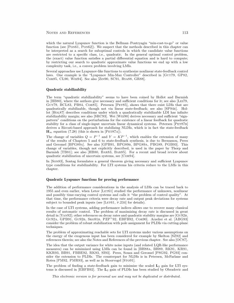
Notes and References 113
which the natural Lyapunov function is the Bellman–Pontryagin “min-cost-to-go” or valuefunction (see [Pon61, Pon62]). We suspect that the methods described in this chapter canbe interpreted as a search for suboptimal controls in which the candidate value functionsare restricted to a specific class, i.e., quadratic. In the general optimal control problem,the (exact) value function satisfies a partial differential equation and is hard to compute;by restricting our search to quadratic approximate value functions we end up with a lowcomplexity task, i.e., a convex problem involving LMIs.
Several approaches use Lyapunov-like functions to synthesize nonlinear state-feedback controllaws. One example is the “Lyapunov Min-Max Controller” described in [Gut79, GP82,Cor85, CL90, Wei94]. See also [Zin90, SC91, Rya88, GR88].
Quadratic stabilizability
The term “quadratic stabilizability” seems to have been coined by Hollot and Barmishin [HB80], where the authors give necessary and sufficient conditions for it; see also [Lei79,Gut79, BCL83, PB84, Cor85]. Petersen [Pet85], shows that there exist LDIs that arequadratically stabilizable, though not via linear state-feedback; see also [SP94e]. Hol-lot [Hol87] describes conditions under which a quadratically stabilizable LDI has infinitestabilizability margin; see also [SRC93]. Wei [Wei90] derives necessary and sufficient “sign-pattern” conditions on the perturbations for the existence of a linear feedback for quadraticstability for a class of single-input uncertain linear dynamical systems. Petersen [Pet87b]derives a Riccati-based approach for stabilizing NLDIs, which is in fact the state-feedbackH∞ equation (7.28) (this is shown in [Pet87a]).
The change of variables Q = P−1 and Y = KP−1, which enables the extension of manyof the results of Chapters 5 and 6 to state-feedback synthesis, is due to Bernussou, Peresand Geromel [BPG89a]. See also [GPB91, BPG89b, BPG89a, PBG89, PGB93]. Thischange of variables, though not explicitly described, is used in the paper by Thorp andBarmish [TB81]; see also [HB80, Bar83, Bar85]. For a recent and broad review aboutquadratic stabilization of uncertain systems, see [Cor94].
In [Son83], Sontag formulates a general theorem giving necessary and sufficient Lyapunovtype conditions for stabilizability. For LTI systems his criteria reduce to the LMIs in thischapter.
Quadratic Lyapunov functions for proving performance
The addition of performance considerations in the analysis of LDIs can be traced back to1955 and even earlier, when Letov [Let61] studied the performance of unknown, nonlinearand possibly time-varying control systems and calls it “the problem of control quality”. Atthat time, the performance criteria were decay rate and output peak deviations for systemssubject to bounded peak inputs (see [Let61, p.234] for details).
In the case of LTI systems, adding performance indices allows one to recover many classicalresults of automatic control. The problem of maximizing decay rate is discussed in greatdetail in [Yan92]; other references on decay rates and quadratic stability margins are [Gu92b,Gu92a, GPB91, Gu92b, Sko91b, PZP+92, EBFB92, Cor90]. Arzelier et al. [ABG93]consider the problem of robust stabilization with pole assignment for PLDIs via cutting-planetechniques.
The problem of approximating reachable sets for LTI systems under various assumptions onthe energy of the exogenous input has been considered for example by Skelton [SZ92] andreferences therein; see also the Notes and References of the previous chapter. See also [OC87].
The idea that the output variance for white noise inputs (and related LQR-like performancemeasures) can be minimized using LMIs can be found in [BH88a, BH89, RK91, KR91,KKR93, BB91, FBBE92, RK93, SI93]. Peres, Souza and Geromel [PSG92, PG93] con-sider the extension to PLDIs. The counterpart for NLDIs is in Petersen, McFarlane andRotea [PM92, PMR93], as well as in Stoorvogel [Sto91].
The problem of finding a state-feedback gain to minimize the scaled L2 gain for LTI sys-tems is discussed in [EBFB92]. The L2 gain of PLDIs has been studied by Obradovic and
This electronic version is for personal use and may not be duplicated or distributed.
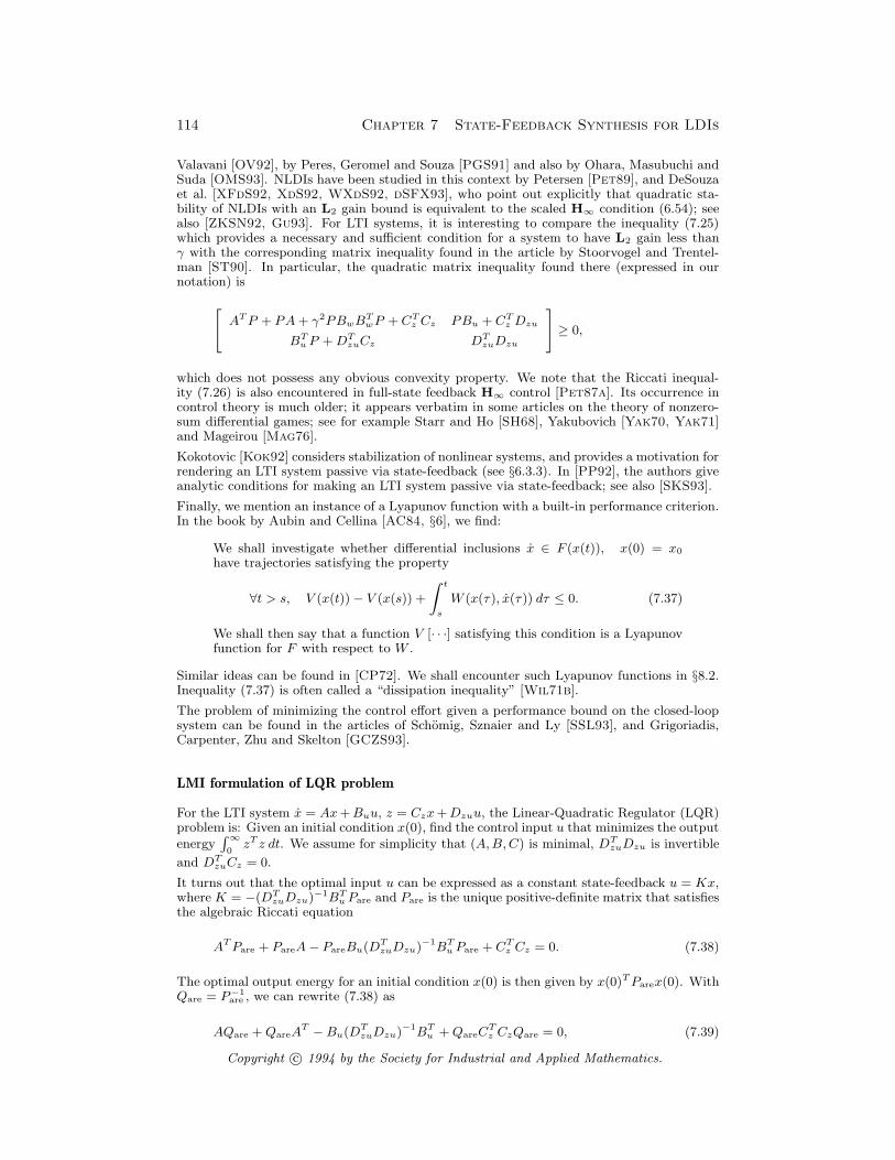
114 Chapter 7 State-Feedback Synthesis for LDIs
Valavani [OV92], by Peres, Geromel and Souza [PGS91] and also by Ohara, Masubuchi andSuda [OMS93]. NLDIs have been studied in this context by Petersen [Pet89], and DeSouzaet al. [XFdS92, XdS92, WXdS92, dSFX93], who point out explicitly that quadratic sta-bility of NLDIs with an L2 gain bound is equivalent to the scaled H∞ condition (6.54); seealso [ZKSN92, Gu93]. For LTI systems, it is interesting to compare the inequality (7.25)which provides a necessary and sufficient condition for a system to have L2 gain less thanγ with the corresponding matrix inequality found in the article by Stoorvogel and Trentel-man [ST90]. In particular, the quadratic matrix inequality found there (expressed in ournotation) is
[
ATP + PA+ γ2PBwBTwP + CT
z Cz PBu + CTz Dzu
BTu P +DT
zuCz DTzuDzu
]
≥ 0,
which does not possess any obvious convexity property. We note that the Riccati inequal-ity (7.26) is also encountered in full-state feedback H∞ control [Pet87a]. Its occurrence incontrol theory is much older; it appears verbatim in some articles on the theory of nonzero-sum differential games; see for example Starr and Ho [SH68], Yakubovich [Yak70, Yak71]and Mageirou [Mag76].
Kokotovic [Kok92] considers stabilization of nonlinear systems, and provides a motivation forrendering an LTI system passive via state-feedback (see §6.3.3). In [PP92], the authors giveanalytic conditions for making an LTI system passive via state-feedback; see also [SKS93].
Finally, we mention an instance of a Lyapunov function with a built-in performance criterion.In the book by Aubin and Cellina [AC84, §6], we find:
We shall investigate whether differential inclusions x ∈ F (x(t)), x(0) = x0have trajectories satisfying the property
∀t > s, V (x(t))− V (x(s)) +
∫ t
s
W (x(τ), x(τ)) dτ ≤ 0. (7.37)
We shall then say that a function V [· · ·] satisfying this condition is a Lyapunovfunction for F with respect to W .
Similar ideas can be found in [CP72]. We shall encounter such Lyapunov functions in §8.2.Inequality (7.37) is often called a “dissipation inequality” [Wil71b].
The problem of minimizing the control effort given a performance bound on the closed-loopsystem can be found in the articles of Schomig, Sznaier and Ly [SSL93], and Grigoriadis,Carpenter, Zhu and Skelton [GCZS93].
LMI formulation of LQR problem
For the LTI system x = Ax+Buu, z = Czx+Dzuu, the Linear-Quadratic Regulator (LQR)problem is: Given an initial condition x(0), find the control input u that minimizes the outputenergy
∫∞
0zT z dt. We assume for simplicity that (A,B,C) is minimal, DT
zuDzu is invertible
and DTzuCz = 0.
It turns out that the optimal input u can be expressed as a constant state-feedback u = Kx,where K = −(DT
zuDzu)−1BT
u Pare and Pare is the unique positive-definite matrix that satisfiesthe algebraic Riccati equation
ATPare + PareA− PareBu(DTzuDzu)
−1BTu Pare + CT
z Cz = 0. (7.38)
The optimal output energy for an initial condition x(0) is then given by x(0)TParex(0). WithQare = P−1are , we can rewrite (7.38) as
AQare +QareAT −Bu(D
TzuDzu)
−1BTu +QareC
Tz CzQare = 0, (7.39)
Copyright c© 1994 by the Society for Industrial and Applied Mathematics.
Notes and References 115
and the optimal output energy as x(0)TQ−1arex(0).
In section §7.4.1, we considered the closely related problem of finding a state-feedback gainK that minimizes an upper bound on the energy of the output, given an initial condition.For LTI systems, the upper bound equals the output energy, and we showed that in this case,the minimum output energy was given by minimizing x(0)TQ−1x(0) subject to Q > 0 and
[
AQ+QAT +BuY + Y TBTu (CzQ+DzuY )T
CzQ+DzuY −I
]
≤ 0. (7.40)
Of course, the optimal value of this EVP must equal the optimal output energy given viathe solution to the Riccati solution (7.39); the Riccati equation can be thus be interpreted asyielding an analytic solution to the EVP. We can derive this analytic solution for the EVP viathe following steps. First, it can be shown, using a simple completion-of-squares argumentthat LMI (7.40) holds for some Q > 0 and Y if and only if it holds for Y = −(DT
zuDzu)−1BT
u ;in this case, Q > 0 must satisfy
QAT +AQ+QCTz CzQ−Bu
(
DTzuDzu
)−1BTu ≤ 0. (7.41)
Next, it can be shown by standard manipulations that if Q > 0 satisfies (7.41), then Q ≤ Qare.Therefore for every initial condition x(0), we have x(0)TQ−1arex(0) ≤ x(0)TQ−1x(0), andtherefore the optimal value of the EVP is just x(0)TQ−1arex(0), and the optimal state-feedbackgain is Kopt = YoptQ
−1are = −(DT
zuDzu)−1BT
u Pare.
It is interesting to note that with P = Q−1, the EVP is equivalent to minimizing x(0)TPx(0)subject to
ATP + PA+ CTz Cz − PBu
(
DTzuDzu
)−1BTu P ≤ 0, (7.42)
which is not a convex constraint in P . However, the problem of maximizing x(0)TPx(0)subject P > 0 and the constraint
ATP + PA− PBu(DTzuDzu)
−1BTu P + CzC
Tz ≥ 0,
which is nothing other than (7.42), but with the inequality reversed, is an EVP; it is well-known (see for example [Wil71b]) that this EVP is another formulation of the LQR problem.
Static versus dynamic state-feedback
An LTI system can be stabilized using dynamic state-feedback if and only if it can be stabi-lized using static state-feedback (see for example, [Kai80]). In fact, similar statements canbe made for all the properties and for all the LDIs considered in this chapter, provided theproperties are specified using quadratic Lyapunov functions. We will demonstrate this facton one simple problem considered in this chapter.
Consider the LTI system
x = Ax+Buu+Bww, x(0) = 0, z = Czx. (7.43)
From §7.5.1, the exists a static state-feedback u = Kx such that the L2 gain from w to zdoes not exceed γ if the LMI in variables Q > 0 and Y is feasible:
[
AQ+QAT +BuY + Y TBTu +BwB
Tw QCT
z
CzQ −γ2I
]
≤ 0.
This electronic version is for personal use and may not be duplicated or distributed.
116 Chapter 7 State-Feedback Synthesis for LDIs
(In fact this condition is also necessary, but this is irrelevant to the current discussion.)Eliminating Y , we get the equivalent LMI in Q > 0 and scalar σ:
AQ+QAT +BwBTw +
QCTz CzQ
γ2≤ σBuB
Tu . (7.44)
We next consider a dynamic state-feedback for the system:
xc = Acxc +Bcx, xc(0) = 0, u = Ccxc +Dcx. (7.45)
We will show that there exist matrices Ac, Bc, Cc and Dc such that the L2 gain of thesystem (7.43,7.45) does not exceed γ if and only if the LMI (7.44) holds. This will establishthat the smallest upper bound on the L2 gain, provable via quadratic Lyapunov functions,is the same irrespective of whether a static state-feedback or a dynamic state-feedback isemployed.
We will show only the part that is not obvious. With state vector xcl = [xT xTc ]T , the
closed-loop system is
xcl = Aclxcl +Bclu, xcl(0) = 0, z = Cclxcl,
where Acl = Abig +BbigKbig with
Abig =
[
A 0
0 0
]
, Bbig =
[
0 Bu
I 0
]
, Kbig =
[
Bc Ac
Dc Cc
]
,
Bcl =
[
Bw
0
]
, Ccl = [Cz 0] .
From §6.3.2, the L2 gain of the closed-loop system does not exceed γ if the LMI in Pbig > 0is feasible:
[
ATbigP + PbigA+ PBbigKbig +KT
bigBTbigP + CT
clCcl PBcl
BTclP −γ2I
]
≤ 0.
Eliminating Kbig from this LMI yields two equivalent LMIs in Pbig > 0 and a scalar τ .
[
ATbigP + PbigA− τI + CT
clCcl PBcl
BTclP −γ2I
]
≤ 0,
[
ATbigP + PbigA− τPBbigBT
bigP + CTclCcl PBcl
BTclP −γ2I
]
≤ 0.
It is easy to verify that the first LMI holds for large enough τ , while the second reduces toτ > 0 and
AQ11 +Q11AT +
BwBTw
γ2+Q11CzC
Tz Q11 ≤ τBuB
Tu ,
where Q11 is the leading n×n block of P−1big . The last LMI is precisely (7.44) with the change
of variables Q = γ2Q11 and σ = γ2τ .
A similar result is established [PZP+92]; other references that discuss the question of whendynamic or nonlinear feedback does better than static feedback include Petersen, Khar-gonekar and Rotea [Pet85, KPR88, RK88, KR88, Pet88, RK89].
Copyright c© 1994 by the Society for Industrial and Applied Mathematics.
Notes and References 117
Dynamic output-feedback for LDIs
A natural extension to the results of this chapter is the synthesis of output-feedback to meetvarious performance specifications. We suspect, however, that output-feedback synthesisproblems have high complexity and are therefore unlikely to be recast as LMI problems.Several researchers have considered such problems: Steinberg and Corless [SC85], Galimidiand Barmish [GB86], and Geromel, Peres, de Souza and Skelton [PGS93]; see also [HCM93].
One variation of this problem is the “reduced-order controller problem”, that is, finding dy-namic output-feedback controllers with the smallest possible number of states. It is shownin [PZPB91, EG93, Pac94] that this problem can be reduced to the problem of minimizingthe rank of a matrix P ≥ 0 subject to certain LMIs. The general problem of minimizing therank of a matrix subject to an LMI constraint has high complexity; in fact, a special rankminimization problem can be shown to be equivalent to the NP-hard zero-one linear pro-gramming problem (see e.g. [Dav94]). Nevertheless several researchers have tried heuristic,local algorithms for such problems and report practical success. Others studying this topicinclude Iwasaki, Skelton, Geromel and de Souza [IS93b, ISG93, GdSS93, SIG93].
Observer-based controllers for nonlinear systems
We prove that the LMIs (7.33) and (7.34) (in the variables P > 0, Q > 0, W and Y ) ensurethe existence of an observer-based controller of the form (7.31) which makes the system (7.30)quadratically stable.
We start by rewriting the system (7.32) in the coordinates x, x− x:[
˙x
˙x− x
]
=
[
LCy(x− x) + f(x) +BuKx
f(x)− f(x) + LCy(x− x)
]
. (7.46)
Using the results of §4.3, we can write
[
˙x
˙x− x
]
∈ Co
Aij
∣
∣ 1 ≤ i ≤M, 1 ≤ j ≤M
[
x
x− x
]
with
Aij =
[
Ai +BuK LCy
0 Aj + LCy
]
, i, j = 1, . . . ,M.
Simple state-space manipulations show the system (7.32) is quadratically stable if and only ifthe system (7.46) is quadratically stable. Therefore, the system (7.32) is quadratically stable
if there exists P > 0 such that
ATijP + P Aij < 0, i, j = 1, . . . ,M. (7.47)
We will now show that the LMI (7.47) has a solution if and only if the LMIs (7.33) and (7.34)do.
First suppose that (7.47) has a solution P . With P partitioned as n× n blocks,
P =
[
P11 P12
PT12 P22
]
,
we easily check that the inequality (7.47) implies
(Ai +BuK)TP11 + P11(Ai +BuK) < 0, i = 1, . . . ,M. (7.48)
This electronic version is for personal use and may not be duplicated or distributed.
118 Chapter 7 State-Feedback Synthesis for LDIs
With the change of variables Q = P−111 and Y = BuQ, the inequality (7.48) is equivalentto (7.33).
Define Q = P−1. The inequality (7.47) becomes
AijQ+ QATij < 0, i, j = 1, . . . ,M.
Denoting by Q22 the lower-right n× n block of Q, we see that this inequality implies
(Ai + LCy)Q22 +Q22(Ai + LCy)T < 0, i = 1, . . . ,M. (7.49)
With P = Q−122 and W = PL, the inequality (7.49) is equivalent to (7.34).
Conversely, suppose that P , Q, Y and W satisfy the LMIs (7.34) and (7.33) and defineL = P−1W , K = Y Q−1. We now prove there exists a positive λ such that
P =
[
λQ−1 0
0 P
]
satisfies (7.47) and therefore proves the closed-loop system (7.32) is quadratically stable. Wecompute
ATijP + P Aij =
λ
(
(Ai +BuK)TQ−1
+Q−1(Ai +BuK)
)
λQ−1LCy
λ(LCy)TQ−1
(Aj + LCy)TP
+ P (Aj + LCy)
,
for i, j = 1, . . . ,M . Therefore, using Schur complements, the closed-loop system (7.32) isquadratically stable if λ > 0 satisfies
λ(Q−1LCy((Aj + LCy)TP + P (Aj + LCy))
−1(LCy)TQ−1)
− (A+BuK)TQ−1 −Q−1(A+BuK) > 0
for i, j = 1, . . . ,M . This condition is satisfied for any λ > 0 such that
λ min1≤j≤M
µj > max1≤i≤M
νi,
where
µj = λmin(Q−1LCy((Aj + LCy)
TP + P (Aj + LCy))−1(LCy)
TQ−1), j = 1, . . . ,M
and
νi = λmax((Ai +BuK)TQ−1 +Q−1(Ai +BuK)), i = 1, . . . ,M.
Since (7.34) and (7.33) are satisfied, such a λ always exists.
Problems of observer-based controller design along with quadratic Lyapunov functions thatprove stability have been considered by Bernstein and Haddad [BH93] and Yaz [Yaz93].
Gain-scheduled or parameter-dependent controllers
Several researchers have extended the results on state-feedback synthesis to handle the casein which the controller parameters can depend on system parameters. Such controllers arecalled gain-scheduled or parameter-dependent. We refer the reader to the articles cited forprecise explanations of what these control laws are, and which design problems can be recastas LMI problems. Lu, Zhou and Doyle in [LZD91] and Becker and Packard [Bec93, BP91]consider the problem in the context of NLDIs. Other relevant references include [PB92,Pac94, PBPB93, BPPB93, GA94, IS93a, IS93b, AGB94].
Copyright c© 1994 by the Society for Industrial and Applied Mathematics.
Chapter 8
Lur’e and Multiplier Methods
8.1 Analysis of Lur’e Systems
We consider the Lur’e system
x = Ax+Bpp+Bww, q = Cqx,
z = Czx, pi(t) = φi(qi(t)), i = 1, . . . , np,(8.1)
where p(t) ∈ Rnp , and the functions φi satisfy the [0, 1] sector conditions
0 ≤ σφi(σ) ≤ σ2 for all σ ∈ R, (8.2)
or, equivalently,
φi(σ)(φi(σ)− σ) ≤ 0 for all σ ∈ R.
The data in this problem are the matrices A, Bp, Bw, Cq and Cz. The results thatfollow will hold for any nonlinearities φi satisfying the sector conditions. In caseswhere the φi are known, however, the results can be sharpened.
It is possible to handle the more general sector conditions
αiσ2 ≤ σφi(σ) ≤ βiσ
2 for all σ ∈ R,
where αi and βi are given. Such systems are readily transformed to the form givenin (8.1) and (8.2) by a loop transformation (see the Notes and References).
An important special case of (8.1), (8.2) occurs when the functions φi are linear,i.e., φi(σ) = δiσ, where δi ∈ [0, 1]. In the terminology of control theory, this is referredto as a system with unknown-but-constant parameters. It is important to distinguishthis case from the PLDI obtained with (8.1), φi(σ) = δi(t)σ and δi(t) ∈ [0, 1], whichis referred to as a system with unknown, time-varying parameters.
Our analysis will be based on Lyapunov functions of the form
V (ξ) = ξTPξ + 2
np∑
i=1
λi
∫ Ci,qξ
0
φi(σ) dσ, (8.3)
where Ci,q denotes the ith row of Cq. Thus the data describing the Lyapunov functionare the matrix P and the scalars λi, i = 1, . . . , np. We require P > 0 and λi ≥ 0,which implies that V (ξ) ≥ ξTPξ > 0 for nonzero ξ.
Note that the Lyapunov function (8.3) depends on the (not fully specified) non-linearities φi. Thus the data P and λi should be thought of as providing a recipe for
119
120 Chapter 8 Lur’e and Multiplier Methods
constructing a specific Lyapunov function given the nonlinearities φi. As an exam-ple, consider the special case of a system with unknown-but-constant parameters, i.e.,φi(σ) = δiσ. The Lyapunov function will then have the form
V (ξ) = ξT(
P + CTq ∆ΛCq
)
ξ
where ∆ = diag(δ1, . . . , δnp) and Λ = diag(λ1, . . . , λnp
). In other words, we are reallysynthesizing a parameter-dependent quadratic Lyapunov function for our parameter-dependent system.
8.1.1 Stability
We set the exogenous input w to zero, and seek P and λi such that
dV (x)
dt< 0 for all nonzero x satisfying (8.1) and (8.2). (8.4)
Since
dV (x)
dt= 2
(
xTP +
np∑
i=1
λipiCi,q
)
(Ax+Bpp) ,
condition (8.4) holds if and only if(
ξTP +
np∑
i=1
λiπiCi,q
)
(Aξ +Bpπ) < 0
for all nonzero ξ satisfying
πi(πi − ci,qξ) ≤ 0, i = 1, . . . , np. (8.5)
It is easily shown that
(ξ, π) | ξ 6= 0, (8.5) = (ξ, π) | ξ 6= 0 or π 6= 0, (8.5) .The S-procedure then yields the following sufficient condition for (8.4): The LMI inP > 0, Λ = diag(λ1, . . . , λnp
) ≥ 0 and T = diag(τ1, . . . , τnp) ≥ 0
[
ATP + PA PBp +ATCTq Λ + CT
q T
BTp P + ΛCqA+ TCq ΛCqBp +BT
p CTq Λ− 2T
]
< 0 (8.6)
holds.
Remark: When we set Λ = 0 we obtain the LMI[
ATP + PA PBp + CTq T
BTp P + TCq −2T
]
< 0,
which can be interpreted as a condition for the existence of a quadratic Lyapunovfunction for the Lur’e system, as follows. Perform a loop transformation on theLur’e system to bring the nonlinearities to sector [−1, 1]. Then the LMI aboveis the same (to within a scaling of the variable T ) as one that yields quadraticstability of the associated DNLDI; see §5.1.
Remark: Condition (8.6) is only a sufficient condition for the existence of a Lur’eLyapunov function that proves stability of system (8.1). It is also necessary whenthere is only one nonlinearity, i.e., when np = 1.
Copyright c© 1994 by the Society for Industrial and Applied Mathematics.
8.1 Analysis of Lur’e Systems 121
8.1.2 Reachable sets with unit-energy inputs
We consider the set reachable with unit-energy inputs,
Rue ∆=
x(T )
∣
∣
∣
∣
∣
∣
∣
∣
x, w satisfy (8.3), x(0) = 0
∫ T
0
wTw dt ≤ 1, T ≥ 0
.
The set
F =
ξ
∣
∣
∣
∣
∣
ξTPξ + 2
np∑
i=1
λi
∫ Ci,qξ
0
φi(σ) dσ ≤ 1
contains Rue ifd
dtV (x) ≤ wTw for all x and w satisfying (8.1) and (8.2). (8.7)
From the S-procedure, the condition (8.7) holds if there exists T = diag(τ1, . . . , τnp) ≥
0 such that
ATP + PA PBp +ATCTq Λ + CT
q T PBw
BTp P + ΛCqA+ TCq ΛCqBp +BT
p CTq Λ− 2T ΛCqBw
BTwP BT
wCTq Λ −I
≤ 0 (8.8)
holds, where Λ = diag(λ1, . . . , λnp) ≥ 0.
Of course, the ellipsoid E = ξ ∈ Rn∣
∣ ξTPξ ≤ 1 contains F , so that E ⊇F ⊇ Rue. Therefore, E gives an outer approximation of Rue if the nonlinearitiesare not known. If the nonlinearities φi are known, F gives a possibly better outerapproximation. We can use these results to prove that a point x0 does not belong tothe reachable set by solving appropriate LMIPs.
8.1.3 Output energy bounds
We consider the system (8.1) with initial condition x(0), and compute upper boundson the output energy
J =
∫ ∞
0
zT z dt
using Lyapunov functions V of the form (8.3).If
d
dtV (x) + zT z ≤ 0 for all x satisfying (8.1), (8.9)
then J ≤ V (x(0)). The condition (8.9) is equivalent to
2
(
ξTP +
np∑
i=1
λiπiCi,q
)
(Aξ +Bpπ) + ξTCTz Czξ ≤ 0,
for every ξ satisfying
πi(πi − ci,qξ) ≤ 0, i = 1, . . . , np.
This electronic version is for personal use and may not be duplicated or distributed.
122 Chapter 8 Lur’e and Multiplier Methods
Using the S-procedure, we conclude that the condition (8.9) holds if there existsT = diag(τ1, . . . , τnp
) ≥ 0 such that[
ATP + PA+ CTz Cz PBp +ATCT
q Λ + CTq T
BTp P + ΛCqA+ TCq ΛCqBp +BT
p CTq Λ− 2T
]
≤ 0. (8.10)
Since V (x(0)) ≤ x(0)T (P + CTq ΛCq)x(0), an upper bound on J is obtained
by solving the following EVP in the variables P , Λ = diag(λ1, . . . , λnp) and T =
diag(τ1, . . . , τnp):
minimize x(0)T(
P + CTq ΛCq
)
x(0)
subject to (8.10), T ≥ 0, Λ ≥ 0, P > 0
If the nonlinearities φi are known, we can obtain possibly better bounds on J bymodifying the objective in the EVP appropriately.
8.1.4 L2 gain
We assume that Dzw = 0 for simplicity. If there exists a Lyapunov function of theform (8.3) and γ ≥ 0 such that
d
dtV (x) ≤ γ2wTw − zT z for all x and w satisfying (8.1), (8.11)
then the L2 gain of the system (8.1) does not exceed γ. The condition (8.11) isequivalent to
2
(
ξTP +
np∑
i=1
λiπiCi,q
)
(Aξ +Bpπ) ≤ γ2wTw − ξTCTz Czξ
for any ξ satisfying πi(πi − ci,qξ) ≤ 0, i = 1, . . . , np. Using the S-procedure, this issatisfied if there exists T = diag(τ1, . . . , τnp
) ≥ 0 such that
ATP + PA+ CTz Cz PBp +ATCT
q Λ + CTq T PBw
BTp P + ΛCqA+ TCq ΛCqBp +BT
p CTq Λ− 2T ΛCqBw
BTwP BT
wCTq Λ −γ2I
≤ 0. (8.12)
The smallest upper bound on the L2 gain, provable using Lur’e Lyapunov functions,is therefore obtained by minimizing γ over γ, P , Λ and T subject to P > 0, Λ =diag(λ1, . . . , λnp
) ≥ 0, T = diag(τ1, . . . , τnp) ≥ 0 and (8.12). This is an EVP.
8.2 Integral Quadratic Constraints
In this section we consider an important variation on the NLDI, in which the point-wise constraint p(t)T p(t) ≤ q(t)T q(t) is replaced with a constraint on the integrals ofp(t)T p(t) and q(t)T q(t):
x = Ax+Bpp+Buu+Bww,
q = Cqx+Dqpp+Dquu+Dqww,
z = Czx+Dzpp+Dzuu+Dzww∫ t
0
p(τ)T p(τ) dτ ≤∫ t
0
q(τ)T q(τ) dτ.
(8.13)
Copyright c© 1994 by the Society for Industrial and Applied Mathematics.
8.2 Integral Quadratic Constraints 123
Such a system is closely related to the NLDI with the same data matrices; indeed,every trajectory of the associated NLDI is a trajectory of (8.13). This system isnot, however, a differential inclusion. In control theory terms, the system (8.13) isdescribed as a linear system with (dynamic) nonexpansive feedback. An importantexample is when p and q are related by a linear system, i.e.,
xf = Afxf +Bfq, p = Cfxf +Dfq, xf (0) = 0,
where ‖Df + Cf (sI −Af )−1Bf‖∞ ≤ 1.
We can also consider a generalization of the DNLDI, in which we have compo-nentwise integral quadratic constraints. Moreover, we can consider integral quadraticconstraints with different sector bounds; as an example we will encounter constraintsof the form
∫ t
0p(τ)T q(τ) dτ ≥ 0 in §8.3.
We will now show that many of the results on NLDIs (and DNLDIs) from Chap-ters 5–7 generalize to systems with integral quadratic constraints. We will demon-strate this generalization for stability analysis and L2 gain bounds, leaving others tothe reader.
As in Chapters 5–7, our analysis will be based on quadratic functions of the stateV (ξ) = ξTPξ, and roughly speaking, the very same LMIs will arise. However, theinterpretation of V is different here. For example, in stability analysis, the V ofChapters 5–7 decreases monotonically to zero. Here, the very same V decreases tozero, but not necessarily monotonically. Thus, V is not a Lyapunov function in theconventional sense.
8.2.1 Stability
Consider system (8.13) without w and z. Suppose P > 0 and λ ≥ 0 are such that
d
dtxTPx < λ
(
pT p− qT q)
, (8.14)
or
d
dt
(
xTPx+ λ
∫ t
0
(
q(τ)T q(τ)− p(τ)T p(τ))
dτ
)
< 0.
Note that the second term is always nonnegative. Using standard arguments fromLyapunov theory, it can be shown that limt→∞ x(t) = 0, or the system is stable.
Now, let us examine the condition (8.14). It is exactly the same as the conditionobtained by applying the S-procedure to the condition
d
dtxTPx < 0, whenever pT p ≤ qT q,
which in turn, leads to the LMI condition for quadratic stability of NLDI (5.3)
P > 0, λ ≥ 0,
ATP + PA+ λCTq Cq PBp + λCT
q Dqp
(PBp + λCTq Dqp)
T −λ(I −DTqpDqp)
< 0.
8.2.2 L2 gain
We assume that x(0) = 0 and, for simplicity, that Dzw = 0 and Dqp = 0.
This electronic version is for personal use and may not be duplicated or distributed.

124 Chapter 8 Lur’e and Multiplier Methods
Suppose P > 0 and λ ≥ 0 are such that
d
dtxTPx < λ
(
pT p− qT q)
+ γ2wTw − zT z. (8.15)
Integrating both sides from 0 to T ,
x(T )TPx(T ) + λ
∫ T
0
(
q(τ)T q(τ)− p(τ)T p(τ))
dτ <
∫ T
0
(
γ2wTw − zT z)
dt.
This implies that the L2 gain from w to z for system (8.13) does not exceed γ.Condition (8.15) leads to the same LMI (6.55) which guarantees that the L2 gainof the NLDI (4.9) from w to z does not exceed γ.
Remark: Almost all the results described in Chapters 5, 6 and 7 extend imme-diately to systems with integral quadratic constraints. The only exceptions arethe results on coordinate transformations (§5.1.1, also §7.2.2), and on reachablesets with unit-peak inputs (§6.1.3 and §7.3.3).
8.3 Multipliers for Systems with Unknown Parameters
We consider the system
x = Ax+Bpp+Bww, q = Cqx+Dqpp,
pi = δiqi, i = 1, . . . , np, z = Czx+Dzww,(8.16)
where p(t) ∈ Rnp , and δi, i = 1, . . . , np are any nonnegative numbers. We can considerthe more general case when αi ≤ δi ≤ βi using a loop transformation (see the Notesand References).
For reasons that will become clear shortly, we begin by defining np LTI systemswith input qi and output qm,i, where qm,i(t) ∈ R:
xm,i = Am,ixm,i +Bm,iqi, xm,i(0) = 0,
qm,i = Cm,ixm,i +Dm,iqi,(8.17)
where we assume that Am,i is stable and (Am,i, Bm,i) is controllable. We furtherassume that
∫ t
0
qi(τ)qm,i(τ) dτ ≥ 0 for all t ≥ 0.
This last condition is equivalent to passivity of the LTI systems (8.17), which in turnis equivalent to the existence of Pi ≥ 0, i = 1, . . . , np, satisfying
[
ATm,iPi + PiAm,i PiBm,i − CT
m,i
BTm,iPi − Cm,i −
(
Dm,i +DTm,i
)
]
≤ 0, i = 1, . . . , np. (8.18)
(See §6.3.3.)Thus, q and qm
∆= [qm,1, . . . , qm,np
]T are the input and output respectively of thediagonal system with realization
Am = diag(Am,i), Bm = diag(Bm,i), Cm = diag(Cm,i), Dm = diag(Dm,i),
Copyright c© 1994 by the Society for Industrial and Applied Mathematics.

8.3 Multipliers for Systems with Unknown Parameters 125
Defining
A =
[
A 0
BmCq Am
]
, Bp =
[
Bp
BmDqp
]
, Bw =
[
Bw
0
]
,
Cq = [DmCq Cm], Dqp = DmDqp, Cz = [Cz 0].
consider the following system with integral quadratic constraints:
dx
dt= Ax+ Bpp+ Bww,
qm = Cqx+ Dqpp,
z = Czx+ Dqpp+Dzww,∫ t
0
pi(τ)qm,i(τ) dτ ≥ 0, i = 1, . . . , np.
(8.19)
It is easy to show that if x is a trajectory of (8.16), then [xT xTm]T is a trajectoryof (8.19) for some appropriate xm. Therefore, conclusions about (8.16) have implica-tions for (8.19). For instance, if system (8.19) is stable, so is system (8.16).
8.3.1 Stability
Consider system (8.19) without w and z. Suppose P > 0 is such that
d
dtxTPx+ 2
np∑
i=1
piqm,i < 0, (8.20)
or
d
dt
(
xTPx+ 2
np∑
i=1
∫ t
0
pi(τ)qm,i(τ) dτ
)
< 0.
Then, it can be shown using standard arguments that limt→∞ x(t) = 0, i.e., thesystem (8.19) is stable.
Condition (8.20) is just the LMI in P > 0, Cm and Dm:[
ATP + PA PBp + CTq
BTp P + Cq Dqp + DT
qp
]
< 0. (8.21)
Remark: LMI (8.21) can also be interpreted as a positive dissipation con-dition for the LTI system with transfer matrix G(s) = −W (s)H(s), whereW (s) = Cm(sI−Am)−1Bm+Dm and H(s) = Cq(sI−A)−1Bp+Dqp. Therefore,we conclude that system (8.16) is stable if there exists a passive W such that−W (s)H(s) has positive dissipation. Hence W is often called a “multiplier”. Seethe Notes and References for details.
8.3.2 Reachable sets with unit-energy inputs
The set of reachable states with unit-energy inputs for the system
x = Ax+Bpp+Bww, q = Cqx+Dqpp,
p = δq, δ ≥ 0,(8.22)
This electronic version is for personal use and may not be duplicated or distributed.
126 Chapter 8 Lur’e and Multiplier Methods
is
Rue ∆=
x(T )
∣
∣
∣
∣
∣
∣
∣
∣
x, w satisfy (8.22), x(0) = 0
∫ T
0
wTw dt ≤ 1, T ≥ 0
.
We can obtain a sufficient condition for a point x0 to lie outside the reachable set Rue,using quadratic functions for the augmented system. Suppose P > 0 is such that
d
dtxTPx+ 2
np∑
i=1
piqm,i < wTw, (8.23)
or
xTPx+ 2
np∑
i=1
∫ t
0
pi(τ)qm,i(τ) dτ <
∫ t
0
w(τ)Tw(τ) dτ.
then the set E =
x∣
∣ xTPx ≤ 1
contains the reachable set for the system (8.19).Condition (8.23) is equivalent to the LMI in P > 0, Cm and Dm:
ATP + PA PBw PBp + CTq
BTwP −I 0
BTp P + Cq 0 Dqp + DT
qp
< 0. (8.24)
Now, the point x0 lies outside the set of reachable states for the system (8.22) ifthere exists P satisfying (8.23) and there exists no z such that
[
x0
z
]T
P
[
x0
z
]
≤ 1.
Partitioning P conformally with the sizes of x0 and z as
P =
[
P11 P12
PT12 P22
]
,
we note that
minz
[
x0
z
]T [
P11 P12
PT12 P22
][
x0
z
]
= xT0 (P11 − P12P−122 P
T12)x0.
Therefore, x0 does not belong to the reachable set for the system (8.22) if there existP > 0, Pi ≥ 0, λ ≥ 0, Cm, and DM satisfying (8.18), (8.24) and
[
xT0 P11x0 − 1 xT0 P12
PT12x0 P22
]
> 0.
This is an LMIP.
Notes and References
Lur’e systems
The Notes and References of Chapters 5 and 7 are relevant to this chapter as well. Lur’eand Postnikov were the first to propose Lyapunov functions consisting of a quadratic form
Copyright c© 1994 by the Society for Industrial and Applied Mathematics.
Notes and References 127
plus the integral of the nonlinearity [LP44]. The book [Lur57] followed this article, in whichthe author showed how to solve the problem of finding such Lyapunov functions analyti-cally for systems of order 2 or 3. Another early book that uses such Lyapunov functions isLetov [Let61]. Work on this topic was continued by Popov [Pop62], Yakubovich [Yak64].Tsypkin [Tsy64d, Tsy64c, Tsy64a, Tsy64b], Szego [Sze63] and Meyer [Mey66]. Juryand Lee [JL65] consider the case of Lur’e systems with multiple nonlinearities and derive acorresponding stability criterion. See also [IR64].
The ellipsoid method is used to construct Lyapunov functions for the Lur’e stability problemin the papers by Pyatnitskii and Skorodinskii [PS82, PS83]. See also [Sko91a, Sko91b] forgeneral numerical methods to prove stability of nonlinear systems via the Popov or circlecriterion. A precursor is the paper by Karmarkar and Siljak [KS75], who used a locally con-vergent algorithm to determine margins for a Lur’e-Postnikov system with one nonlinearity.
Indeed, in the early books by Lur’e, Postnikov, and Letov the problem of constructing Lya-punov functions reduces to the satisfaction of some inequalities. In some special cases theyeven point out geometrical properties of the regions defined by the inequalities, i.e., that theyform a parallelogram. But as far as we know, convexity of the regions is not noted in theearly work. In any case, it was not known in the 1940’s and 1950’s that solution of convexinequalities is practically and theoretically tractable.
Construction of Lyapunov functions for systems with integral quadratic constraints
We saw in §8.2.1 that the quadratic positive function V (ξ) = ξTPξ is not necessarily aLyapunov function in the conventional sense for the system (8.13) with integral quadraticconstraints; although V (x(t))→ 0 as t→∞, it does not do so monotonically. We now showhow we can explicitly construct a Lyapunov function given P , in cases when p and q arerelated by
xf = f(xf , q, t), p = g(xf , q, t), (8.25)
where xf (t) ∈ Rnf .
Since∫ t
0pT pdτ ≤
∫ t
0qT q dτ , it can be shown (see for example [Wil72]) that Vf : Rnf → R+
given by
Vf (ξf )∆= sup
−∫ T
0
(
qT q − pT p)
dt
∣
∣
∣
∣
xf (0) = ξf , xf satisfies (8.25), T ≥ 0
is a Lyapunov function that proves stability of system (8.25). Moreover, the Lyapunovfunction V : Rn ×Rnf → R+ given by
V (ξ, ξf )∆= ξTPξ + Vf (ξf )
proves stability of the interconnection
x = Ax+Bpp, q = Cqx+Dqpp,
xf = f(xf , q, t), p = g(xf , q, t).
Note that this construction also shows that ξTPξ proves the stability of the NLDI (5.2).
Integral quadratic constraints have recently received much attention, especially in the formerSoviet Union. See for example [Yak88, Meg92a, Meg92b, Yak92, Sav91, SP94b, SP94h,SP94d].
Systems with constant, unknown parameters
Problems involving system (8.16) are widely studied in the field of robust control, sometimesunder the name “real-µ problems”; see Siljak [Sil89] for a survey. The results of §8.3 were
This electronic version is for personal use and may not be duplicated or distributed.
128 Chapter 8 Lur’e and Multiplier Methods
derived by Fan, Tits and Doyle in [FTD91] using an alternate approach, involving the ap-plication of an off-axis circle criterion (see also §3.3). We also mention [TV91], where Tesiand Vicino study a hybrid system, consisting of a Lur’e system with unknown parameters.
There are elegant analytic solutions for some very special problems involving parameter-dependent linear systems, e.g., Kharitonov’s theorem [Kha78] and its extensions [BHL89].A nice survey of these results can be found in Barmish [Bar93].
Complexity of stabilization problems
The stability (and performance) analysis problems considered in §8.3 have high complexity.For example, checking if (8.16) is stable is NP-hard (see Coxson and Demarco [CD91], Braatzand Young [BYDM93], Poljak and Rohn [PR94], and Nemirovskii [Nem94]). We conjecturethat checking whether a general DNLDI is stable is also NP-hard.
Likewise, many stabilization problems for uncertain systems are NP-hard. For instance, theproblem of checking whether system (8.16) is stabilizable by a constant state-feedback canbe shown to be NP-hard using the method of [Nem94].
A related result, due to Blondel and Gevers [BG94], states that checking whether thereexists a common stabilizing LTI controller for three LTI systems is undecidable. In contrast,checking whether there exists a static, output-feedback control law for a single LTI systemis rationally decidable [ABJ75].
Multiplier methods
See [Wil69a, NT73, DV75, Sil69, Wil70, Wil76] for discussion of and bibliography onmultiplier theory and its connections to Lyapunov stability theory. In general multipliertheory we consider the system
x = Ax+Bpp+Bww, q = Cqx+Dqpp, p(t) = ∆(q, t).
The method involves checking that Hm =W(
Cq(sI −A)−1Bp +Dqp
)
satisfies
Hm(jω) +Hm(jω)∗ ≥ 0 for every ω ∈ R,
for some choice of W from a set that is determined by the properties of ∆. When ∆ isa nonlinear time-invariant memoryless operator satisfying a sector condition (i.e., when wehave a Lur’e system), the multipliers W are of the form (1 + qs) for some q ≥ 0. This isthe famous Popov criterion [Pop62, Pop64]; we must also cite Yakubovich, who showed,using the S-procedure [Yak77], that feasibility of LMI (8.6) is equivalent to the existence ofq nonnegative such that (1 + qs)(cq(sI −A)−1bp) + 1/k has positive dissipation.
In the case when ∆(q, t) = δq(t) for some unknown real number δ, the multiplier W can beany passive transfer matrix. This observation was made by Brockett and Willems in [BW65];given a transfer function Hqp they show that the transfer function Hqp/(1+kHqp) is stable forall values of k in (0,∞) if and only if there exists a passive multiplier W such that WHqp isalso passive. This case has also been considered in [CS92b, SC93, SL93a, SLC94] where theauthors devise appropriate multipliers for constant real uncertainties. The paper [BHPD94]by Balakrishnan et al., shows how various stability tests for uncertain systems can be red-erived in the context of multiplier theory, and how these tests can be reduced to LMIPs. Seealso [LSC94].
Safonov and Wyetzner use a convex parametrization of multipliers found by Zames andFalb [ZF68, ZF67] to prove stability of systems subject to “monotonic” or “odd-monotonic”nonlinearities (see [SW87] for details; see also [GG94]). Hall and How, along with Bern-stein and Haddad, generalize the use of quadratic Lyapunov functions along with multipliersfor various classes of nonlinearities, and apply them to Aerospace problems; see for ex-ample [HB91a, How93, HH93b, HHHB92, HH93a, HHH93a, HCB93, HB93b, HB93a,HHH93b]. See also [CHD93].
Copyright c© 1994 by the Society for Industrial and Applied Mathematics.
Notes and References 129
Multiple nonlinearities for Lur’e systems
Our analysis method for Lur’e systems with multiple nonlinearities in §8.1 can be conser-vative, since the S-procedure can be conservative in this case. Rapoport [Rap86, Rap87,Rap88] devises a way of determining if there exists Lyapunov functions of the form (8.3)nonconservatively by generating appropriate LMIs. We note, however, that the number ofthese LMIs grows exponentially with the number of nonlinearities. Kamenetskii [Kam89]and Rapoport [Rap89] derive corresponding frequency-domain stability criteria. Kamenet-skii calls his results “convolution method for solving matrix inequalities”.
Loop transformations
Consider the Lur’e system with general sector conditions, i.e.,
x = Ax+Bp, q = Cx+Dp,
pi(t) = φi(qi(t)), αiσ2 ≤ σφi(σ) ≤ βiσ2.
(8.26)
Here we have dropped the variables w and z and the subscripts on B, C and D to simplifythe presentation. We assume this system is well-posed, i.e., det(I −D∆) 6= 0 for all diagonal∆ with αi ≤ ∆ii ≤ βi.Define
pi∆=
1
βi − αi(φi(qi)− αiqi) = φi(qi).
It is readily shown that 0 ≤ σφi(σ) ≤ σ2 for all σ. Let Λ and Γ denote the diagonal matrices
Λ = diag(α1, . . . , αnq ), Γ = diag(β1 − α1, . . . , βnq − αnq ),
so that p = Γ−1(p − Λq). We now substitute p = Γp + Λq into (8.26) and, using our well-posedness assumption, solve for x and q in terms of x and p. This results in
x =(
A+BΛ(I −DΛ)−1C)
x+B(I − ΛD)−1Γp,
q = (I −DΛ)−1Cx+ (I −DΛ)−1DΓp.
We can therefore express (8.26) as
x = Ax+ Bp, q = Cx+ Dp,
pi(t) = φi(qi(t)), 0 ≤ σφi(σ) ≤ σ2.(8.27)
where
A = A+BΛ(I −DΛ)−1C, B = B(I − ΛD)−1Γ,
C = (I −DΛ)−1C, D = (I −DΛ)−1DΓ.
Note that (8.27) is in the standard Lur’e system form. So to analyze the more general Lur’esystem (8.26), we simply apply the methods of §8.1 to the loop-transformed system (8.27).In practice, i.e., in a numerical implementation, it is probably better to derive the LMIsassociated with the more general Lur’e system than to loop transform to the standard Lur’esystem.
The construction above is a loop transformation that maps nonlinearities in sector [αi, βi]into the standard sector, i.e., [0, 1]. Similar transformations can be used to map any set ofsectors into any other, including so-called infinite sectors, in which, say, βi = +∞.
The term loop transformation comes from a simple block-diagram interpretation of the equa-tions given above. For detailed descriptions of loop transformations, see the book by Desoerand Vidyasagar [DV75, p50].
This electronic version is for personal use and may not be duplicated or distributed.

Chapter 9
Systems with Multiplicative Noise
9.1 Analysis of Systems with Multiplicative Noise
9.1.1 Mean-square stability
We first consider the discrete-time stochastic system
x(k + 1) =
(
A0 +
L∑
i=1
Aipi(k)
)
x(k), (9.1)
where p(0), p(1), . . ., are independent, identically distributed random variables with
E p(k) = 0, E p(k)p(k)T = Σ = diag(σ1, . . . , σL). (9.2)
We assume that x(0) is independent of the process p.Define M(k), the state correlation matrix, as
M(k)∆= Ex(k)x(k)T .
Of course, M satisfies the linear recursion
M(k + 1) = AM(k)AT +
L∑
i=1
σ2iAiM(k)ATi , M(0) = Ex(0)x(0)T . (9.3)
If this linear recursion is stable, i.e., regardless of x(0), limk→∞M(k) = 0, we saythe system is mean-square stable. Mean-square stability implies, for example, thatx(k)→ 0 almost surely.
It can be shown (see the Notes and References) that mean-square stability isequivalent to the existence of a matrix P > 0 satisfying the LMI
ATPA− P +L∑
i=1
σ2iATi PAi < 0. (9.4)
An alternative, equivalent condition is that the dual inequality
AQAT −Q+
L∑
i=1
σ2iAiQATi < 0 (9.5)
holds for some Q > 0.
131
132 Chapter 9 Systems with Multiplicative Noise
Remark: For P > 0 satisfying (9.4), we can interpret the function V (ξ) = ξTPξas a stochastic Lyapunov function: EV (x) decreases along trajectories of (9.1).Alternatively, the function V (M) = TrMP is a (linear) Lyapunov function forthe deterministic system (9.3) (see the Notes and References).
Remark: Mean-square stability can be verified directly by solving the Lyapunovequation in P
ATPA− P +
L∑
i=1
σ2iATi PAi + I = 0
and checking whether P > 0. Thus the LMIPs (9.4) and (9.5) offer no computa-tional (or theoretical) advantages for checking mean-square stability.
We can consider variations on the mean-square stability problem, for example,determining the mean-square stability margin. Here, we are given A0, . . . , AL, andasked to find the largest γ such that with Σ < γ2I, the system (9.1) is mean-squarestable. From the LMIP characterizations of mean-square stability, we can deriveGEVP characterizations that yield the exact mean-square stability margin. Again,the GEVP offers no computational or theoretical advantages, since the mean-squarestability margin can be obtained by computing the eigenvalue of a (large) matrix.
9.1.2 State mean and covariance bounds with unit-energy inputs
We now add an exogenous input w to our stochastic system:
x(k + 1) = Ax(k) +Bww(k) +
L∑
i=1
(Aix(k) +Bw,iw(k)) pi(k), x(0) = 0. (9.6)
We assume that the exogenous input w is deterministic, with energy not exceedingone, i.e.,
∞∑
k=0
w(k)Tw(k) ≤ 1.
Let x(k) denote the mean of x(k), which satisfies x(k+1) = Ax(k)+Bww(k), and let
X(k) denote the covariance of x(k), i.e., X(k) = E (x(k)− x(k)) (x(k)− x(k))T. We
will develop joint bounds on x(k) and X(k).Suppose V (ξ) = ξTPξ where P > 0 satisfies
EV (x(k + 1)) ≤ EV (x(k)) + w(k)Tw(k) (9.7)
for all trajectories. Then,
EV (x(k)) ≤k∑
j=0
w(j)Tw(j), k ≥ 0,
which implies that, for all k ≥ 0,
Ex(k)TPx(k) = x(k)TP x(k) + E (x(k)− x(k))TP (x(k)− x(k))
= x(k)TP x(k) + TrX(k)P
≤ 1.
Copyright c© 1994 by the Society for Industrial and Applied Mathematics.

9.1 Analysis of Systems with Multiplicative Noise 133
Let us now examine condition (9.7). We note that
EV (x(k + 1)) =
[
x(k)
w(k)
]T
M
[
x(k)
w(k)
]
+Tr
(
ATPA+
L∑
i=1
σ2iATi PAi
)
X(k),
where
M =
[
AT
BTw
]
P[
A Bw
]
+
L∑
i=1
σ2i
[
ATi
BTw,i
]
P[
Ai Bw,i
]
.
Next, the LMI conditions[
AT
BTw
]
P[
A Bw
]
+
L∑
i=1
σ2i
[
ATi
BTw,i
]
P[
Ai Bw,i
]
≤[
P 0
0 I
]
(9.8)
and
ATPA+
L∑
i=1
σ2iATi PAi < P (9.9)
imply
EV (x(k + 1)) ≤ xT (k)P x(k) + w(k)Tw(k)
+Tr
(
ATPA+L∑
i=1
σ2iATi PAi
)
X(k)
≤ xT (k)P x(k) + w(k)Tw(k)
+E (x(k)− x(k))TP (x(k)− x(k))
= EV (x(k)) + w(k)Tw(k), k ≥ 0.
Of course, LMI (9.8) implies LMI (9.9); thus, we conclude that LMI (9.8) im-plies (9.7). Therefore, we conclude that x(k) and X(k) must belong to the set
( ¯x(k), X(k))∣
∣ x(k)TP x(k) + TrX(k)P ≤ 1
for any P > 0 satisfying the LMI (9.8). For example, we have the bound TrM(k)P ≤ 1on the state covariance matrix.
We can derive further bounds on M(k). For example, since we have TrM(k)P ≤λmin(P )TrM(k) and therefore TrM(k) ≤ 1/λmin(P ), we can derive bounds on TrMby maximizing λmin(P ) subject to (9.8) and P > 0. This is an EVP. As anotherexample, we can derive an upper bound on λmax(M) by maximizing TrP subjectto (9.8) and P > 0, which is another EVP.
9.1.3 Bound on L2 gain
We now consider the system
x(k + 1) = Ax(k) +Bww(k) +
L∑
i=1
(Aix(k) +Bw,iw(k)) pi(k), x(0) = 0,
z(k) = Czx(k) +Dzww(k) +
L∑
i=1
(Cz,ix(k) +Dzw,iw(k)) pi(k).
(9.10)
This electronic version is for personal use and may not be duplicated or distributed.
134 Chapter 9 Systems with Multiplicative Noise
with the same assumptions on p. We assume that w is deterministic.We define the L2 gain η of this system as
η2∆= sup
E
∞∑
k=0
z(k)T z(k)
∣
∣
∣
∣
∣
∞∑
k=0
w(k)Tw(k) ≤ 1
. (9.11)
Suppose that V (ξ) = ξTPξ, with P > 0, satisfies
EV (x(k + 1))−EV (x(k)) ≤ γ2w(k)Tw(k)−E z(k)T z(k). (9.12)
Then γ ≥ η. The condition (9.12) can be shown to be equivalent to the LMI[
A Bw
Cz Dzw
]T [
P 0
0 I
][
A Bw
Cz Dzw
]
−[
P 0
0 γ2I
]
+
L∑
i=1
σ2i
[
Ai Bw,i
Cz,i Dzw,i
]T [
P 0
0 I
][
Ai Bw,i
Cz,i Dzw,i
]
≤ 0.
(9.13)
Minimizing γ subject to LMI (9.13), which is an EVP, yields an upper bound on η.
Remark: It is straightforward to apply the scaling method developed in §6.3.4to obtain componentwise results.
9.2 State-Feedback Synthesis
We now add a control input u to our system:
x(k + 1) = Ax(k) +Buu(k) +Bww(k)+L∑
i=1
(Aix(k) +Bu,iu(k) +Bw,iw(k)) pi(k),
z(k) = Czx(k) +Dzuu(k) +Dzww(k)+L∑
i=1
(Cz,ix(k) +Dzu,iu(k) +Dzw,iw(k)) pi(k).
(9.14)
We seek a state-feedback u(k) = Kx(k) such that the closed-loop system
x(k + 1) = (A+BuK)x(k) +Bww(k)+L∑
i=1
((Ai +Bu,iK)x(k) +Bw,iw(k)) pi(k),
z(k) = (Cz +DzuK)x(k) +Dzww(k)+L∑
i=1
((Cz,i +Dzu,iK)x(k) +Dzw,iw(k)) pi(k),
(9.15)
satisfies various properties.
9.2.1 Stabilizability
We seek K and Q > 0 such that
(A+BuK)Q(A+BuK)T −Q
+
L∑
i=1
σ2i (Ai +Bu,iK)Q(Ai +Bu,iK)T < 0.
Copyright c© 1994 by the Society for Industrial and Applied Mathematics.
9.2 State-Feedback Synthesis 135
With the change of variable Y = KQ, we obtain the equivalent condition
(AQ+BuY )Q−1(AQ+BuY )T −Q
+
L∑
i=1
σ2i (AiQ+Bu,iY )Q−1(AiQ+Bu,iY )T < 0,(9.16)
which is easily written as an LMI in Q and Y .Thus, system (9.14) is mean-square stabilizable (with constant state-feedback) if
and only if the LMI Q > 0, (9.16) is feasible. In this case, a stabilizing state-feedbackgain is K = Y Q−1.
As an extension, we can maximize the closed-loop mean-square stability margin.System (9.15) is mean-square stable for Σ ≤ γ2I if and only if
(AQ+BuY )Q−1(AQ+BuY )T −Q
+γ2L∑
i=1
(AiQ+Bu,iY )Q−1(AiQ+Bu,iY )T < 0(9.17)
holds for some Y and Q > 0. Therefore, finding K that maximizes γ reduces to thefollowing GEVP:
maximize γ
subject to Q > 0, (9.17)
9.2.2 Minimizing the bound on L2 gain
We now seek a state-feedback gain K which minimizes the bound on L2 gain (asdefined by (9.11)) for system (9.15). η ≤ γ for some K if there exist P > 0 and Ksuch that
L∑
i=1
σ2i
[
Ai +Bu,iK Bw,i
Cz,i +Dzu,iK Dzw,i
]T
P
[
Ai +Bu,iK Bw,i
Cz,i +Dzu,iK Dzw,i
]
+
[
A+BuK Bw
Cz +DzuK Dzw
]T
P
[
A+BuK Bw
Cz +DzuK Dzw
]
≤[
P 0
0 γ2I
]
where
P =
[
P 0
0 I
]
.
We make the change of variables Q = P−1, Y = KQ. Applying a congruencewith Q = diag(Q, I), we get
L∑
i=1
σ2i
[
AiQ+Bu,iY Bw,i
Cz,iQ+Dzu,iY Dzw,i
]T
Q−1
[
AiQ+Bu,iY Bw,i
Cz,iQ+Dzu,iY Dzw,i
]
+
[
AQ+BuY Bw
CzQ+DzuY Dzw
]T
Q−1
[
AQ+BuY Bw
CzQ+DzuY Dzw
]
≤[
Q 0
0 γ2I
]
.
This inequality is readily transformed to an LMI.
This electronic version is for personal use and may not be duplicated or distributed.
136 Chapter 9 Systems with Multiplicative Noise
Notes and References
Systems with multiplicative noise
Systems with multiplicative noise are a special case of stochastic systems. For an introductionto this topic see Arnold [Arn74] or Astrom [Ast70].
A rigorous treatment of continuous-time stochastic systems requires much technical machin-ery (see [EG94]). In fact there are many ways to formulate the continuous-time version of asystem such as (9.10); see Ito [Ito51] and Stratonovitch [Str66].
Stability of system with multiplicative noise
For a survey of different concepts of stability for stochastic systems see [Koz69] and thereferences therein. The definition of mean-square stability can be found in [Sam59]. Mean-square stability is a strong form of stability. In particular, it implies stability of the meanEx(k) and that all trajectories converge to zero with probability one [Kus67, Wil73]. For thesystems considered here, it is also equivalent to L2-stability, which is the property that (see
for example, [EP92]) E∑T
t=0‖x(t)‖2 has a (finite) limit as T →∞ for all initial conditions.
The equation for the state correlation matrix (9.3) can be found in [McL71, Wil73]. An alge-braic criterion for mean-square stability of a system with multiplicative white noise is givenin [NS72]. It is reminiscent of the classical (deterministic) Hurwitz criterion. Frequency-domain criteria are given in [WB71]. The related Lyapunov equation was given by Klein-mann [Kle69] for the case L = 1 (i.e., a single uncertainty). The criterion then reducesto an H2 norm condition on a certain transfer matrix. (This is in parallel with the resultsof [EP92], see below.)
Kats and Krasovskii introduced in [KK60] the idea of a stochastic Lyapunov function andproved a related Lyapunov theorem. A thorough stability analysis of (nonlinear) stochasticsystems was made by Kushner in [Kus67] using this idea of a stochastic Lyapunov func-tion. Kushner used this idea to derive bounds for return time, expected output energy, etc.However, this approach does not provide a way to construct the Lyapunov functions.
Proof of stability criterion
We now prove that condition (9.4) is a necessary and sufficient condition for mean-squarestability. We first prove that condition (9.4) is sufficient. Let P > 0 satisfy (9.4). Introducethe (linear Lyapunov) function V (M) = TrMP , which is positive on the cone of nonnegativematrices. For nonzero M(k) satisfying (9.3),
V (M(k + 1)) = Tr
(
AM(k)AT +
L∑
i=1
σ2iAiM(k)ATi
)
P
= TrM(k)
(
ATPA+
L∑
i=1
σ2iATi PAi
)
< TrM(k)P = V (M(k)).
A further standard argument from Lyapunov theory proves that M(k) converges to zero ask →∞.
To prove that condition (9.4) is also necessary, we assume that the system is mean-squarestable. This means that for every positive initial condition M(0) ≥ 0, the solution to thelinear recursion (9.3) goes to zero as k → 0. Linearity of system (9.3) implies that, for anarbitrary choice ofM(0), the corresponding solutionM(k) converges to 0, i.e., (9.3) is stable.We now write (9.3) as m(k+1) = Am(k), where m(k) is a vector containing the n2 elementsof M(k), and A is a real matrix. (This matrix can be expressed via Kronecker products
Copyright c© 1994 by the Society for Industrial and Applied Mathematics.
Notes and References 137
involving A0, . . . , AL.) Stability of A is equivalent to that of AT , and the correspondingmatrix difference equation,
N(k + 1) = ATN(k)A+
L∑
i=1
σ2iATi N(k)Ai, (9.18)
is also stable.
Now let N(0) > 0, and let N(k) be the corresponding solution of (9.18). Since N(k) satisfiesa stable first-order linear difference equation with constant coefficients, the function
P (k) =
k∑
j=0
N(j)
has a (finite) limit for k →∞, which we denote by P . The fact that N(0) > 0 implies P > 0.
Now (9.18) implies
P (k + 1) = N(0) +ATP (k)A+
L∑
i=1
σ2iATi P (k)Ai
Taking the limit k →∞ shows that P satisfies (9.4).
Mean-square stability margin
System (9.10) can be viewed as a linear system subject to random parameter variations. Forsystems with deterministic parameters only known to lie in ranges, the computation of anexact stability margin is an NP-hard problem [CD92]. The fact that a stochastic analogof the deterministic stability margin is easier to compute should not be surprising; we aredealing with a very special form of stability, which only considers the average behavior of thesystem.
An exact stability margin can also be computed for continuous-time systems with multiplica-tive noise provided the Ito framework is considered; see [EG94]. In contrast, the computationof an exact stability margin seems difficult for Stratonovitch systems.
In [EP92], El Bouhtouri and Pritchard provide a complete robustness analysis in a slightlydifferent framework than ours, namely for so-called “block-diagonal” perturbations. Roughlyspeaking, they consider a continuous-time Ito system of the form
dx(t) = Ax(t)dt+
L∑
i=1
Bi∆i(Cx(t))dpi(t),
where the operators ∆i are Lipschitz continuous, with ∆i(0) = 0; the processes pi, i =1, . . . , L, are standard Brownian motions (which, roughly speaking, are integrals of whitenoise).
We note that our framework can be recovered by assuming that the operators ∆i are restrictedto a diagonal structure of the form ∆i(z) = σiz.
Measuring the “size” of the perturbation term by(∑L
i=1‖∆i‖2
)1/2, where ‖ · ‖ denotes the
Lipschitz norm, leads the authors of [EP92] to the robustness margin
minimize γ
subject to P > 0, ATP + PA+ CTC < 0, BTi PBi ≤ γ, i = 1, . . . , L
This electronic version is for personal use and may not be duplicated or distributed.

138 Chapter 9 Systems with Multiplicative Noise
For L = 1, and B1 and C are vectors, that is, when a single scalar uncertain parameterperturbs an LTI system, both this result and ours coincide with the H2 norm of (A,B1, C).This is consistent with the earlier results of Kleinmann [Kle69] and Willems [WB71] (seealso [BB91, p114] for a related result). For L > 1 however, applying their results to ourframework would be conservative, since we only consider “diagonal” perturbations with “re-peated elements”, ∆i = σiI. Note that the LMI approach can also solve the state-feedbacksynthesis problem in the framework of [EP92]. El Bouhtouri and Pritchard provide a solutionof this problem in [EP94].
Stability conditions for arbitrary noise intensities are given in geometric terms in [WW83].In our framework, this happens if and only if the optimal value of the corresponding GEVPis zero.
Bounds on state covariance with noise input
We consider system (9.6) in which w is a unit white noise process, i.e., w(k) are independent,identically distributed with Ew(k) = 0, Ew(k)w(k)T = W , and w is independent of p.In this case, of course, the state mean x is zero. We derive an upper bound on the statecorrelation (or covariance) of the system.
The state correlation M(k) satisfies the difference equation
M(k + 1) = AM(k)AT +BwWBTw +
L∑
i=1
σ2i(
AiM(k)ATi +Bw,iWBT
w,i
)
,
with M(0) = 0.
Since the system is mean-square stable, the state correlation M(k) has a (finite) limit M∞
which satisfies
M∞ = AM∞AT +BwWBT
w +
L∑
i=1
σ2i(
AiM∞ATi +Bw,iWBT
w,i
)
.
In fact, the matrix M∞ can be computed directly as the solution of a linear matrix equation.However, the above LMI formulation extends immediately to more complicated situations (forinstance, when the white noise input w has a covariance matrix with unknown off-diagonalelements), while the “direct” method does not. See the Notes and References for Chapter 6for details on how these more complicated situations can be handled.
Extension to other stochastic systems
The Lur’e stability problem considered in §8.1 can be extended to the stochastic framework;see Wonham [Won66]. This extension can be cast in terms of LMIs.
It is also possible to extend the results in this chapter to “uncertain stochastic systems”, ofthe form
x(k + 1) =
(
A(k) +
L∑
i=1
σiAipi(k)
)
x(k),
where the time-varying matrix A(k) is only known to belong to a given polytope.
State-feedback synthesis
Conditions for stabilizability for arbitrary noise intensities are given in geometric termsin [WW83]. Apart from this work, the bulk of earlier research on this topic concentrated
Copyright c© 1994 by the Society for Industrial and Applied Mathematics.
Notes and References 139
on Linear-Quadratic Regulator theory for continuous-time Ito systems, which addresses theproblem of finding an input u that minimize a performance index of the form
J(K) = E
∫ ∞
0
(
x(t)TQx(t) + u(t)TRu(t))
dt
where Q ≥ 0 and R > 0 are given. The solution of this problem, as found in [McL71]or [Ben92], can be expressed as a (linear, constant) state-feedback u(t) = Kx(t) where thegain K is given in terms of the solution of a non-standard Riccati equation. (See [Kle69,Won68, FR75, BH88b] for additional details.) The existing methods (see e.g. [Phi89,RSH90]) use homotopy algorithms to solve these equations, with no guarantee of global con-vergence. We can solve these non-standard Riccati equations reliably (i.e., with guaranteedconvergence), by recognizing that the solution is an extremal point of a certain LMI feasibilityset.
This electronic version is for personal use and may not be duplicated or distributed.

Chapter 10
Miscellaneous Problems
10.1 Optimization over an Affine Family of Linear Systems
We consider a family of linear systems,
x = Ax+Bww, z = Cz(θ)x+Dzw(θ)w, (10.1)
where Cz and Dzw depend affinely on a parameter θ ∈ Rp. We assume that A isstable and (A, Bw) is controllable. The transfer function,
Hθ(s)∆= Cz(θ)(sI −A)−1Bw +Dzw(θ),
depends affinely on θ.Several problems arising in system and control theory have the form
minimize ϕ0(Hθ)
subject to ϕi(Hθ) < αi, i = 1, . . . , p(10.2)
where ϕi are various convex functionals. These problems can often be recast as LMIproblems. To do this, we will represent ϕi(Hθ) < αi as an LMI in θ, αi, and possiblysome auxiliary variables ζi (for each i):
Fi(θ, αi, ζi) > 0.
The general optimization problem (10.2) can then be expressed as the EVP
minimize α0
subject to Fi(θ, αi, ζi) > 0, i = 0, 1, . . . , p
10.1.1 H2 norm
The H2 norm of the system (10.1), i.e.,
‖Hθ‖22 =1
2πTr
∫ ∞
0
Hθ(jω)∗Hθ(jω) dω,
is finite if and only if Dzw(θ) = 0. In this case, it equals TrCzWcCTz , where Wc > 0 is
the controllability Gramian of the system (10.1) which satisfies (6.6). Therefore, theH2 norm of the system (10.1) is less than or equal to γ if and only if the followingconditions on θ and γ2 are satisfied:
Dzw(θ) = 0, TrCz(θ)WcCz(θ)T ≤ γ2.
The quadratic constraint on θ is readily cast as an LMI.
141

142 Chapter 10 Miscellaneous Problems
10.1.2 H∞ norm
From the bounded-real lemma, we have ‖Hθ‖∞ < γ if and only if there exists P ≥ 0such that
[
ATP + PA PBw
BTwP −γ2I
]
+
[
Cz(θ)T
Dzw(θ)T
]
[
Cz(θ) Dzw(θ)]
≤ 0.
Remark: Here we have converted the so-called “semi-infinite” convex constraint‖Hθ(iω)‖ < γ for all ω ∈ R into a finite-dimensional convex (linear matrix)inequality.
10.1.3 Entropy
The γ-entropy of the system (10.1) is defined as
Iγ(Hθ)∆=
−γ22π
∫ ∞
−∞
log det(I − γ2Hθ(iω)Hθ(iω)∗) dω, if ‖Hθ‖∞ < γ,
∞, otherwise.
When it is finite, Iγ(Hθ) is given by TrBTwPBw, where P is a symmetric matrix
with the smallest possible maximum singular value among all solutions of the Riccatiequation
ATP + PA+ Cz(θ)TCz(θ) +
1
γ2PBwB
TwP = 0.
For the system (10.1), the γ-entropy constraint Iγ ≤ λ is therefore equivalent to anLMI in θ, P = P T , γ2, and λ:
Dzw(θ) = 0,
ATP + PA PBw Cz(θ)T
BTwP −γ2I 0
Cz(θ) 0 −I
≤ 0, TrBT
wPBw ≤ λ.
10.1.4 Dissipativity
Suppose that w and z are the same size. The dissipativity of Hθ (see (6.59)) exceedsγ if and only if the LMI in the variables P = P T and θ holds:
[
ATP + PA PBw − Cz(θ)T
BTwP − Cz(θ) 2γI −Dzw(θ)−Dzw(θ)
T
]
≤ 0.
We remind the reader that passivity corresponds to zero dissipativity.
10.1.5 Hankel norm
The Hankel norm of Hθ is less than γ if and only if the following LMI in Q, θ and γ2
holds:
Dzw(θ) = 0, ATQ+QA+ Cz(θ)TCz(θ) ≤ 0,
γ2I −W1/2c QW
1/2c ≥ 0, Q ≥ 0.
(Wc is the controllability Gramian defined by (6.6).)
Copyright c© 1994 by the Society for Industrial and Applied Mathematics.
10.2 Analysis of Systems with LTI Perturbations 143
10.2 Analysis of Systems with LTI Perturbations
In this section, we address the problem of determining the stability of the system
x = Ax+Bpp, q = Cqx+Dqpp, pi = δi ∗ qi, i = 1, . . . , np, (10.3)
where p = [p1 · · · pnp]T , q = [q1 · · · qnp
]T , and δi, i = 1, . . . , np, are impulseresponses of single-output single-output LTI systems whose H∞ norm is strictly lessthan one, and ∗ denotes convolution. This problem has many variations: Some of theδi may be impulse response matrices, or they may satisfy equality constraints such asδ1 = δ2. Our analysis can be readily extended to these cases.
Let Hqp(s) = Cq(sI−A)−1Bp+Dqp. Suppose that there exists a diagonal transfermatrix W (s) = diag(W1(s), . . . ,Wnp
(s)), where W1(s), . . . ,Wnp(s) are single-input
single-output transfer functions with no poles or zeros on the imaginary axis suchthat
supω∈R
∥
∥W (iω)Hqp(iω)W (iω)−1∥
∥ < 1 (10.4)
Then from a small-gain argument, the system (10.3) is stable. Such a W is referredto as a frequency-dependent scaling .
Condition (10.4) is equivalent to the existence of γ > 0 such that
Hqp(iω)∗W (iω)∗W (iω)Hqp(iω)−W (iω)∗W (iω) + γI ≤ 0,
for all ω ∈ R. From spectral factorization theory, it can be shown that such a Wexists if and only if there exists a stable, diagonal transfer matrix V and positive µsuch that
Hqp(iω)∗(V (iω) + V (iω)∗)Hqp(iω)− (V (iω) + V (iω)∗) + γI ≤ 0,
V (iω) + V (iω)∗ ≥ µI,(10.5)
for all ω ∈ R.In order to reduce (10.5) to an LMI condition, we restrict V to belong to an affine,
finite-dimensional set Θ of diagonal transfer matrices, i.e., of the form
Vθ(s) = DV(θ) + CV(θ)(sI −A)−1B,
where DV and CV are affine functions are θ.Then, Hqp(−s)TVθ(s)Hqp(s) − Vθ(s) has a state-space realization (Aaug , Baug,
Caug(θ), Daug(θ)) where Caug andDaug are affine in θ, and (Aaug, Baug) is controllable.From §10.1.4, the condition that Vθ(iω)+Vθ(iω)
∗ ≥ µI for all ω ∈ R is equivalentto the existence of P1 ≥ 0, θ and γ > 0 such that the LMI
[
ATVP1 + P1AV P1BV − CV(θ)
T
(P1BV − CV(θ)T )T −(DV(θ) +DV(θ)
T ) + µI
]
≤ 0
holds.The condition Hqp(iω)
∗(Vθ(iω) + Vθ(iω)∗)Hqp(iω)− (Vθ(iω) + Vθ(iω)
∗) + γI ≤ 0is equivalent to the existence of P2 = PT
2 and θ satisfying the LMI[
ATaugP2 + P2Aaug P2Baug + Caug(θ)
T
(P2Baug + Caug(θ)T )T Daug(θ) +Daug(θ)
T + γI
]
≤ 0. (10.6)
(See the Notes and References for details.) Thus proving stability of the system (10.3)using a finite-dimensional set of frequency-dependent scalings is an LMIP.
This electronic version is for personal use and may not be duplicated or distributed.

144 Chapter 10 Miscellaneous Problems
10.3 Positive Orthant Stabilizability
The LTI system x = Ax is said to be positive orthant stable if x(0) ∈ Rn+ implies that
x(t) ∈ Rn+ for all t ≥ 0, and x(t) → 0 as t → ∞. It can be shown that the system
x = Ax is positive orthant stable if and only if Aij ≥ 0 for i 6= j, and there existsa diagonal P > 0 such that PAT + AP < 0. Therefore checking positive orthantstability is an LMIP.
We next consider the problem of finding K such that the system x = (A+BK)xis positive orthant stable. Equivalently, we seek a diagonal Q > 0 and K such thatQ(A + BK)T + (A + BK)Q < 0, with the off-diagonal entries of A + BK beingnonnegative. Since Q > 0 is diagonal, the last condition holds if and only if allthe off-diagonal entries of (A+BK)Q are nonnegative. Therefore, with the change ofvariables Y = KQ, proving positive orthant stabilizability for the system x = Ax+Buis equivalent to finding a solution to the LMIP with variables Q and Y :
Q > 0, (AQ+BY )ij ≥ 0, i 6= j, QAT + Y TBT +AQ+BY < 0. (10.7)
Remark: The method can be extended to invariance of more general (polyhedral)sets. Positive orthant stability and stabilizability of LDIs can be handled in asimilar way. See the Notes and References.
10.4 Linear Systems with Delays
Consider the system described by the delay-differential equation
d
dtx(t) = Ax(t) +
L∑
i=1
Aix(t− τi), (10.8)
where x(t) ∈ Rn, and τi > 0. If the functional
V (x, t) = x(t)TPx(t) +
L∑
i=1
∫ τi
0
x(t− s)TPix(t− s) ds, (10.9)
where P > 0, P1 > 0, . . . , PL > 0, satisfies dV (x, t)/dt < 0 for every x satisfying (10.8),then the system (10.8) is stable, i.e., x(t)→ 0 as t→∞.
It can be verified that dV (x, t)/dt = y(t)TWy(t), where
W =
ATP + PA+
L∑
i=1
Pi PA1 · · · PAL
AT1 P −P1 · · · 0
......
. . ....
ATLP 0 · · · −PL
, y(t) =
x(t)
x(t− τ1)...
x(t− τL)
.
Therefore, we can prove stability of system (10.8) using Lyapunov functionals of theform (10.9) by solving the LMIP W < 0, P > 0, P1 > 0, . . . , PL > 0.
Copyright c© 1994 by the Society for Industrial and Applied Mathematics.
10.5 Interpolation Problems 145
Remark: The techniques for proving stability of norm-bound LDIs, discussedin Chapter 5, can also be used on the system (10.8); it can be verified that theLMI (5.15) that we get for quadratic stability of a DNLDI, in the case when thestate x is a scalar, is the same as the LMI W < 0 above. We also note that wecan regard the delay elements of system (10.8) as convolution operators with unitL2 gain, and use the techniques of §10.2 to check its stability.
Next, we add an input u to the system (10.8) and consider
d
dtx(t) = Ax(t) +Bu(t) +
L∑
i=1
Aix(t− τi). (10.10)
We seek a state-feedback u(t) = Kx(t) such that the system (10.10) is stable.From the discussion above, there exists a state-feedback gain K such that a Lya-
punov functional of the form (10.9) proves the stability of the system (10.10), if
W =
(A+BK)TP + P (A+BK) +
L∑
i=1
Pi PA1 · · · PAL
AT1 P −P1 · · · 0
......
. . ....
ATLP 0 · · · −PL
< 0
for some P , P1, . . . , PL > 0.Multiplying every block entry ofW on the left and on the right by P−1 and setting
Q = P−1, Qi = P−1PiP−1 and Y = KP−1, we obtain the condition
X =
AQ+QAT +BY + Y TBT +
L∑
i=1
Qi A1Q · · · ALQ
QAT1 −Q1 · · · 0
......
. . ....
QATL 0 · · · −QL
< 0.
Thus, checking stabilizability of the system (10.8) using Lyapunov functionals of theform (10.9) is an LMIP in the variables Q, Y , Q1, . . . , QL.
Remark: It is possible to use the elimination procedure of §2.6.2 to eliminatethe matrix variable Y and obtain an equivalent LMIP with fewer variables.
10.5 Interpolation Problems
10.5.1 Tangential Nevanlinna-Pick problem
Given λ1, . . . , λm with λi ∈ C+∆= s | Re s > 0 and distinct, u1, . . . , um, with
ui ∈ Cq and v1, . . . , vm, with vi ∈ Cp, i = 1, . . . ,m, the tangential Nevanlinna-Pick
This electronic version is for personal use and may not be duplicated or distributed.

146 Chapter 10 Miscellaneous Problems
problem is to find, if possible, a function H : C −→ Cp×q which is analytic in C+,and satisfies
H(λi)ui = vi, i = 1, . . . ,m, with ‖H‖∞ ≤ 1. (10.11)
Problem (10.11) arises in multi-input multi-output H∞ control theory.From Nevanlinna-Pick theory, problem (10.11) has a solution and only if the Pick
matrix N defined by
Nij =u∗i uj − v∗i vjλ∗i + λj)
is positive semidefinite. N can also be obtained as the solution of the Lyapunovequation
A∗N +NA− (U∗U − V ∗V ) = 0.
where A = diag(λ1, . . . , λm), U = [u1 · · · um], V = [v1 · · · vm]. For future reference,we note that N = Gin −Gout, where
A∗Gin +GinA− U∗U = 0, A∗Gout +GoutA− V ∗V = 0.
Solving the tangential Nevanlinna-Pick problem simply requires checking whetherN ≥0.
10.5.2 Nevanlinna-Pick interpolation with scaling
We now consider a simple variation of problem (10.11): Given λ1, . . . , λm with λi ∈C+, u1, . . . , um, with ui ∈ Cp and v1, . . . , vm, with vi ∈ Cp, i = 1, . . . ,m, the problemis to find
γopt = inf
‖DHD−1‖∞∣
∣
∣
∣
∣
H is analytic in C+, D = D∗ > 0
D ∈ D, H(λi)ui = vi, i = 1, . . . ,m
, (10.12)
where D is the set of m×m block-diagonal matrices with some specified block struc-ture. Problem (10.12) corresponds to finding the smallest scaled H∞ norm of allinterpolants. This problem arises in multi-input multi-output H∞ control synthesisfor systems with structured perturbations.
With a change of variables P = D∗D and the discussion in the previous section,it follows that γopt is the smallest positive γ such that there exists P > 0, P ∈ D suchthat the following equations and inequality hold:
A∗Gin +GinA− U∗PU = 0,
A∗Gout +GoutA− V ∗PV = 0,
γ2Gin −Gout ≥ 0.
This is a GEVP.
10.5.3 Frequency response identification
We consider the problem of identifying the transfer function H of a linear systemfrom noisy measurements of its frequency response at a set of frequencies. We seek Hsatisfying two constraints:
Copyright c© 1994 by the Society for Industrial and Applied Mathematics.
10.6 The Inverse Problem of Optimal Control 147
• Consistency with measurements. For some ni with |ni| ≤ ε, we have fi =H(jωi)+ni. Here, fi is the measurement of the frequency response at frequencyωi, ni is the (unknown) measurement error, and ε is the measurement precision.
• Prior assumption. α-shifted H∞ norm of H does not exceed M .
From Nevanlinna-Pick theory, there exist H and n with H(ωi) = fi + ni satisfyingthese conditions if and only if there exist ni with |ni| ≤ ε, Gin > 0 and Gout > 0 suchthat
M2Gin −Gout ≥ 0,
(A+ αI)∗Gin +Gin (A+ αI)− e∗e = 0,
(A+ αI)∗Gout +Gout (A+ αI)− (f + n)∗(f + n) = 0,
where A = diag(jω1, . . . , jωm), e = [1 · · · 1], f = [f1 · · · fm], and n =[n1 · · · nm]. It can be shown that these conditions are equivalent to
M2Gin −Gout ≥ 0,
(A+ αI)∗Gin +Gin (A+ αI)− e∗e = 0,
(A+ αI)∗Gout +Gout (A+ αI)− (f + n)∗(f + n) ≥ 0,
with |ni| ≤ ε.With this observation, we can answer a number of interesting questions in fre-
quency response identification by solving EVPs and GEVPs.
• For fixed α and ε, minimize M . Solving this GEVP answers the question “Givenα and a bound on the noise values, what is the smallest possible α-shiftedH∞ norm of the system consistent with the measurements of the frequencyresponse?”
• For fixed α and M , minimize ε. Solving this EVP answers the question “Givenα and a bound on α-shifted H∞ norm of the system, what is the “smallest”possible noise such that the measurements are consistent with the given valuesof α and M .
10.6 The Inverse Problem of Optimal Control
Given a system
x = Ax+Bu, x(0) = x0, z =
[
Q1/2 0
0 R1/2
][
x
u
]
,
with (A,B) is stabilizable, (Q,A) is detectable and R > 0, the LQR problem is todetermine u that minimizes
∫ ∞
0
zT z dt.
The solution of this problem can be expressed as a state-feedback u = Kx withK = −R−1BTP , where P is the unique nonnegative solution of
ATP + PA− PBR−1BTP +Q = 0.
The inverse problem of optimal control is the following. Given a matrix K, determineif there exist Q ≥ 0 and R > 0, such that (Q,A) is detectable and u = Kx is the
This electronic version is for personal use and may not be duplicated or distributed.
148 Chapter 10 Miscellaneous Problems
optimal control for the corresponding LQR problem. Equivalently, we seek R > 0 andQ ≥ 0 such that there exists P nonnegative and P1 positive-definite satisfying
(A+BK)TP + P (A+BK) +KTRK +Q = 0, BTP +RK = 0
and ATP1 +P1A < Q. This is an LMIP in P , P1, R and Q. (The condition involvingP1 is equivalent to (Q,A) being detectable.)
10.7 System Realization Problems
Consider the discrete-time minimal LTI system
x(k + 1) = Ax(k) +Bu(k), y(k) = Cx(k), (10.13)
where x : Z+ → Rn, u : Z+ → Rnu y : Z+ → Rny . The system realization problem isto find a change of state coordinates x = T x, such that the new realization
x(k + 1) = T−1ATx(k) + T−1Bu(k) y(k) = CTx(k), (10.14)
satisfies two competing constraints: First, the input-to-state transfer matrix, T−1(zI−A)−1B should be “small”, in order to avoid state overflow in numerical implementa-tion; and second, the state-to-output transfer matrix, C(zI−A)−1T should be “small”,in order to minimize effects of state quantization at the output.
Suppose we assume that the RMS value of the input is bounded by α and requirethe RMS value of the state to be less than one. This yields the bound
∥
∥T−1(zI −A)−1B∥
∥
∞≤ 1/α, (10.15)
where the H∞ norm of the transfer matrix H(z) is defined as
‖H‖∞ = sup ‖H(z)‖ | |z| > 1 .
Next, suppose that the state quantization noise is modeled as a white noise sequencew(k) with Ew(k)Tw(k) = η, injected directly into the state, and its effect on theoutput is measured by its RMS value, which is just η times the H2 norm of thestate-to-output transfer matrix:
pnoise = η∥
∥C(zI −A)−1T∥
∥
2. (10.16)
Our problem is then to compute T to minimize the noise power (10.16) subject to theoverflow avoidance constraint (10.15).
The constraint (10.15) is equivalent to the existence of P > 0 such that[
ATPA− P + T−TT−1 ATPB
BTPA BTPB − I/α2
]
≤ 0.
The output noise power can be expressed as
p2noise = η2TrTTWoT,
where Wo is the observability Gramian of the original system (A,B,C), given by
Wo =
∞∑
k=0
(AT )kCTCAk.
Copyright c© 1994 by the Society for Industrial and Applied Mathematics.
10.7 System Realization Problems 149
Wo is the solution of the Lyapunov equation
ATWoA−Wo + CTC = 0.
With X = T−TT−1, the realization problem is: Minimize η2TrWoX−1 subject
to X > 0 and the LMI (in P > 0 and X)[
ATPA− P +X ATPB
BTPA BTPB − I/α2
]
≤ 0. (10.17)
This is a convex problem in X and P , and can be transformed into the EVP
minimize η2TrYWc
subject to (10.17), P > 0,
[
Y I
I X
]
≥ 0
Similar methods can be used to handle several variations and extensions.
Input u has RMS value bounded componentwise
Suppose the RMS value of each component ui is less than α (instead of the RMS valueof u being less than α) and that the RMS value of the state is still required to be lessthan one. Then, using the methods of §10.9, an equivalent condition is the LMI (withvariables X, P and R):
[
ATPA− P +X ATPB
BTPA BTPB −R/α2
]
≤ 0, P > 0, (10.18)
where R > 0 is diagonal, with unit trace, so that the EVP (over X, Y , P and R) is
minimize η2TrYWc
subject to (10.18), P > 0, X > 0
R > 0, R is diagonal, TrR = 1[
Y I
I X
]
≥ 0
Minimizing state-to-output H∞ norm
Alternatively, we can measure the effect of the quantization noise on the output withthe H∞ norm, that is, we can choose T to minimize ‖C(zI−A)−1T‖∞ subject to theconstraint (10.15). The constraint ‖C(zI − A)−1T‖∞ ≤ γ is equivalent to the LMI(over Y > 0 and X = T−TT−1 > 0):
[
ATY A− Y + CTC ATY
Y A Y −X/α2
]
≤ 0. (10.19)
Therefore choosing T to minimize ‖C(zI −A)−1T‖∞ subject to (10.15) is the GEVP
minimize γ
subject to P > 0, Y > 0, X > 0, (10.17), (10.19)
An optimal state coordinate transformation T is any matrix that satisfies Xopt =(TTT )−1, where Xopt is an optimal value of X in the GEVP.
This electronic version is for personal use and may not be duplicated or distributed.
150 Chapter 10 Miscellaneous Problems
10.8 Multi-Criterion LQG
Consider the LTI system given by
x = Ax+Bu+ w, y = Cx+ v, z =
[
Q1/2 0
0 R1/2
][
x
u
]
,
where u is the control input; y is the measured output; z is the exogenous output;w and v are independent white noise signals with constant, positive-definite spectraldensity matrices W and V respectively; we further assume that Q ≥ 0 and R > 0,that (A,B) is controllable, and that (C,A) and (Q,A) are observable.
The standard Linear-Quadratic Gaussian (LQG) problem is to minimize
Jlqg = limt→∞
E z(t)T z(t)
over u, subject to the condition that u(t) is measurable on y(τ) for τ ≤ t. The optimalcost is given by
J∗lqg = Tr (XlqgU +QYlqg) ,
where Xlqg and Ylqg are the unique positive-definite solutions of the Riccati equations
ATXlqg +XlqgA−XlqgBR−1BTXlqg +Q = 0,
AYlqg + YlqgAT − YlqgC
TV −1CYlqg +W = 0,(10.20)
and U = YlqgCTV −1CYlqg.
In the multi-criterion LQG problem, we have several exogenous outputs of interestgiven by
zi =
[
Q1/2i 0
0 R1/2i
][
x
u
]
, Qi ≥ 0, Ri > 0, i = 0, . . . , p.
We assume that (Q0, A) is observable. For each zi, we associate a cost function
J ilqg = lim
t→∞E zi(t)
T zi(t), i = 0, . . . , p. (10.21)
The multi-criterion LQG problem is to minimize J0lqg over u subject to the measurabil-
ity condition and the constraints J ilqg < γi, i = 1, . . . , p. This is a convex optimization
problem, whose solution is given by maximizing
Tr (XlqgU +QYlqg)−p∑
i=1
γiτi,
over nonnegative τ1, . . . , τp, where Xlqg and Ylqg are the solutions of (10.20) with
Q = Q0 +
p∑
i=1
τiQi and R = R0 +
p∑
i=1
τiRi.
Noting that Xlqg ≥ X for every X > 0 that satisfies
ATX +XA−XBR−1BTX +Q ≥ 0,
we conclude that the optimal cost is the maximum of
Tr
(
XU + (Q0 +
p∑
i=1
τiQi)Ylqg
)
−p∑
i=1
γiτi,
Copyright c© 1994 by the Society for Industrial and Applied Mathematics.

10.9 Nonconvex Multi-Criterion Quadratic Problems 151
over X, τ1, . . . , τp, subject to X > 0, τ1 ≥ 0, . . . , τp ≥ 0 and
ATX +XA−XB
(
R0 +
p∑
i=1
τiRi
)−1
BTX +Q0 +
p∑
i=1
τiQi ≥ 0.
Computing this is an EVP.
10.9 Nonconvex Multi-Criterion Quadratic Problems
In this section, we consider the LTI system x = Ax+Bu, x(0) = x0, where (A,B) iscontrollable. For any u, we define a set of p+ 1 cost indices J0, . . . , Jp by
Ji(u) =
∫ ∞
0
[xT uT ]
[
Qi Ci
CTi Ri
][
x
u
]
dt, i = 0, . . . , p.
Here the symmetric matrices[
Qi Ci
CTi Ri
]
, i = 0, . . . , p,
are not necessarily positive-definite. The constrained optimal control problem is:
minimize J0,
subject to Ji ≤ γi, i = 1, . . . , p, x(t)→ 0 as t→∞(10.22)
The solution to this problem proceeds as follows: We first define
Q = Q0 +
p∑
i=1
τiQi, R = R0 +
p∑
i=1
τiRi, C = C0 +
p∑
i=1
τiCi,
where τ1 ≥ 0, . . . , τp ≥ 0. Next, with τ = [τ1 · · · τp], we define
S(τ, u)∆= J0 +
p∑
i=1
τiJi −p∑
i=1
τiγi.
Then, the solution of problem (10.22), when it is not −∞, is given by:
supτ
infuS(τ, u) | x(t)→ 0 as t→∞
(See the Notes and References.)For any fixed τ , the infimum over u of S(τ, u), when it is not −∞, is computed
by solving the EVP in P = P T
maximize x(0)TPx(0)−p∑
i=1
τiγi
subject to
[
ATP + PA+Q PB + CT
BTP + C R
]
≥ 0
(10.23)
Therefore, the optimal control problem is solved by the EVP in P = P T and τ :
maximize x(0)TPx(0)−p∑
i=1
τiγi
subject to
[
ATP + PA+Q PB + CT
BTP + C R
]
≥ 0, τ1 ≥ 0, . . . , τp ≥ 0.
This electronic version is for personal use and may not be duplicated or distributed.
152 Chapter 10 Miscellaneous Problems
Notes and References
Optimization over an affine family of linear systems
Optimization over an affine family of transfer matrices arises in linear controller design viaYoula’s parametrization of closed-loop transfer matrices; see Boyd and Barratt [BB91] andthe references therein. Other examples include finite-impulse-response (FIR) filter design (seefor example [OKUI88]) and antenna array weight design [KRB89].
In [Kav94] Kavranoglu considers the problem of approximating in the H∞ norm a giventransfer matrix by a constant matrix, which is a problem of the form considered in §10.1. Hecasts the problem as an EVP.
Stability of systems with LTI perturbations
For references about this problem, we refer the reader to the Notes and References in Chap-ter 3. LMI (10.6) is derived from Theorems 3 and 4 in Willems [Wil71b].
Positive orthant stabilizability
The problem of positive orthant stability and holdability was extensively studied by Berman,Neumann and Stern [BNS89, §7.4]. They solve the positive orthant holdability problemwhen the control input is scalar; our results extend theirs to the multi-input case. The studyof positive orthant holdability draws heavily from the theory of positive matrices, referencesfor which are [BNS89] and the book by Berman and Plemmons [BP79, ch6].
Diagonal solutions to the Lyapunov equation play a central role in the positive orthantstabilizability and holdability problems. A related paper is by Geromel [Ger85], who givesa computational procedure to find diagonal solutions of the Lyapunov equation. Diagonalquadratic Lyapunov functions also arise in the study of large-scale systems [MH78]; seealso §3.4. A survey of results and applications of diagonal Lyapunov stability is given inKaszkurewicz and Bhaya [KB93].
A generalization of the concept of positive orthant stability is that of invariance of polyhedralsets. The problem of checking whether a given polyhedron is invariant as well as the associatedstate-feedback synthesis problem have been considered by many authors, see e.g., [Bit88,BBT90, HB91b] and references therein. The LMI method of §10.3 can be extended to thepolyhedral case, using the approach of [CH93]. Finally, we note that the results of §10.3 areeasily generalized to the LDIs considered in Chapter 4.
Stabilization of systems with time delays
The introduction of Lyapunov functionals of the form (10.9) is due to Krasovskii [Kra56].Skorodinskii [Sko90] observed that the problem of proving stability of a system with delaysvia Lyapunov–Krasovskii functionals is a convex problem. See also [PF92, WBL92, SL93b,FBB92].
It is interesting to note that the “structured stability problem” or “µ-analysis problem”can be cast in terms of linear systems with delays. Consider a stable LTI system withtransfer matrix H and L inputs and outputs, connected in feedback with a diagonal transfermatrix ∆ with H∞ norm less than one. This system is stable for all such ∆ if and only ifsup
ω∈R µ(H(jω)) < 1, where µ denotes the structured singular value (see [Doy82]). It can
be shown (see [Boy86]) that if the feedback system is stable for all ∆ which are diagonal,with ∆ii(s) = e−sTi , Ti > 0 (i.e., delays) then the system is stable for all ∆ with ‖∆‖∞ ≤ 1.Thus, verifying sup
ω∈R µ(H(jω)) < 1 can be cast as checking stability of a linear systemwith L arbitrary, positive delays. In particular we see that Krasovskii’s method from 1956can be interpreted as a Lyapunov-based µ-analysis method.
Copyright c© 1994 by the Society for Industrial and Applied Mathematics.
Notes and References 153
Interpolation problems
The classical Nevanlinna-Pick problem dates back at least to 1916 [Pic16, Nev19]. Thereare two matrix versions of this problem: the matrix Nevanlinna-Pick problem [DGK79]and the tangential Nevanlinna-Pick problem [Fed75]. A comprehensive description of theNevanlinna-Pick problem, its extensions and variations can be found in the book by Ball,Gohberg and Rodman [BGR90].
A number of researchers have studied the application of Nevanlinna-Pick theory to problemsin system and control: Delsarte, Genin and Kamp discuss the role of the matrix Nevanlinna-Pick problem in circuit and systems theory [DGK81]. Zames and Francis, in [ZF83], studythe implications of interpolation conditions in controller design; also see [OF85]. Changand Pearson [CP84] solve a class of H∞-optimal controller design problems using matrixNevanlinna-Pick theory. Safonov [Saf86] reduces the design of controllers for systems withstructured perturbations to the scaled matrix Nevanlinna-Pick problem. In [Kim87], Kimurareduces a class of H∞-optimal controller design problems to the tangential Nevanlinna-Pickproblem; see also [Bal94].
System identification
The system identification problem considered in §10.5.3 can be found in [CNF92]. Othersystem identification problems can be cast in terms of LMI problems; see e.g., [PKT+94].
The inverse problem of optimal control
This problem was first considered by Kalman [Kal64], who solved it when the control u isscalar; see also [And66c]. It is discussed in great detail by Anderson and Moore [AM90,§5.6], Fujii and Narazaki [FN84] and the references therein; they solve the problem whenthe control weighting matrix R is known, by checking that the return difference inequality
(
I −BT (−iωI −AT )−1K)
R(
I −KT (iωI −A)−1B)
≥ R
holds for all ω ∈ R. Our result handles the case of unknown R, i.e., the most general formof the inverse optimal control problem.
System realization problems
For a discussion of the problem of system realizations see [MR76, Thi84], which give an-alytical solutions via balanced realizations for special realization problems. The book byGevers and Li [GL93a] describes a number of digital filter realization problems. Liu, Skeltonand Grigoriadis discuss the problem of optimal finite word-length controller implementa-tion [LSG92]. See also Rotea and Williamson [RW94b, RW94a].
We conjecture that the LMI approach to system realization can also incorporate the constraintof stability, i.e., that the (nonlinear) system not exhibit limit cycles due to quantization oroverflow; see, e.g., [Wil74b].
We also note that an H∞ norm constraint on the input-to-state transfer matrix yields,indirectly, a bound on the peak gain from input to state; Boyd and Doyle [BD87]. This canbe used to guarantee no overflow given a maximum peak input level.
Multi-criterion LQG
The multi-criterion LQG problem is discussed in [BB91]; see also the references cited there.Rotea [Rot93] calls this problem “generalized H2 control”. He shows that one can restrictattention to observer-based controllers such as
d
dtx = (A+BK)x+ Y CTV −1(y − Cx), u = Kx,
This electronic version is for personal use and may not be duplicated or distributed.
154 Chapter 10 Miscellaneous Problems
where Y is given by (10.20). The covariance of the residual state x−x is Y and the covarianceP of the state x is given by the solution of the Lyapunov equation:
(A+BK)P + P (A+BK)T + Y CTV −1CY = 0. (10.24)
The value of each cost index J ilqg defined by (10.21) is then
J ilqg = TrRiKPK
T + TrQi (Y + P ) .
Now, taking Z = KP as a new variable, we replace (10.24) by the linear equality in W andP
AP + PAT +BZ + ZTBT + Y CTV −1CY = 0
and each cost index becomes
J ilqg = TrRiZP
−1ZT + TrQi (Y + P ) .
The multi-criterion problem is then solved by the EVP in P , Z and X
minimize TrR0X + TrQ0(P + Y )
subject to
[
X Z
ZT P
]
≥ 0,
AP + PAT +BZ + ZTBT + Y CTV −1CY = 0,
TrRiX + TrQi(P + Y ) ≤ γi, i = 1, . . . , L
This formulation of the multi-criterion LQG problem is the dual of our formulation; the twoformulations can be used together in an efficient primal-dual method (see, e.g., [VB93b]). Wealso mention an algorithm devised by Zhu, Rotea and Skelton [ZRS93] to solve a similar classof problems. For a variation on the multi-criterion LQG problem discussed here, see [Toi84];see also [TM89, Mak91].
Nonconvex multi-criterion quadratic problems
This section is based on Megretsky [Meg92a, Meg92b, Meg93] and Yakubovich [Yak92].In our discussion we omitted important technical details, such as constraint regularity, whichis covered in these articles. Also, Yakubovich gives conditions under which the infimumis actually a minimum (that is, there exists an optimal control law that achieves the bestperformance). The EVP (10.23) is derived from Theorem 3 in Willems [Wil71b].
Many of the sufficient conditions for NLDIs in Chapters 5–7 can be shown to be necessaryand sufficient conditions when we consider integral constraints on p and q, by analyzing themas nonconvex multi-criterion quadratic problems. This is illustrated in the following section.
Mixed H2–H∞ problem
We consider the analog of an NLDI with integral quadratic constraint:
x = Ax+Bpp+Buu, q = Cqx, z =
[
Q1/2 0
0 R1/2
][
x
u
]
∫ ∞
0
pT p dt ≤∫ ∞
0
qT q dt
Copyright c© 1994 by the Society for Industrial and Applied Mathematics.
Notes and References 155
Define the cost function J =∫∞
0zT z dt. Our goal is to determine minK maxp J , over all
possible linear state-feedback strategies u = Kx. (Note that this is the same as the prob-lem considered in §7.4.1 with integral constraints on p and q instead of pointwise in timeconstraints.)
For fixed K, finding the maximum of J over admissible p’s is done using the results of §10.9.This maximum is obtained by solving the EVP
minimize x(0)TPx(0)
subject to
(A+BuK)TP + P (A+BuK)+
Q+KTRK + τCTq Cq
PBp
BTp P −τI
≤ 0, τ ≥ 0
The minimization over K is now simply done by introducing the new variables W = P−1,Y = KW , µ = 1/τ . Indeed, in this particular case, we know we can add the constraintP > 0. The corresponding EVP is then
minimize x(0)TW−1x(0)
subject to
(
WAT + Y BTu +AW +BuY+
WQW + Y TRY +WCTq CqW/µ
)
µBp
µBTp −µI
≤ 0, µ ≥ 0
which is the same as the EVP (7.23).
This electronic version is for personal use and may not be duplicated or distributed.

Notation
R, Rk, Rm×n The real numbers, real k-vectors, real m× n matrices.
R+ The nonnegative real numbers.
C The complex numbers.
Re(a) The real part of a ∈ C, i.e., (a+ a∗)/2.
S The closure of a set S ⊆ Rn.
Ik The k× k identity matrix. The subscript is omitted when k is notrelevant or can be determined from context.
MT Transpose of a matrix M : (MT )ij = Mji.
M∗ Complex-conjugate transpose of a matrixM : (M ∗)ij = M∗ji, where
α∗ denotes the complex-conjugate of α ∈ C.
TrM Trace of M ∈ Rn×n, i.e.,∑n
i=1Mii.
M ≥ 0 M is symmetric and positive semidefinite, i.e., M = MT andzTMz ≥ 0 for all z ∈ Rn.
M > 0 M is symmetric and positive-definite, i.e., zTMz > 0 for all nonzeroz ∈ Rn.
M > N M and N are symmetric and M −N > 0.
M1/2 For M > 0, M1/2 is the unique Z = ZT such that Z > 0, Z2 = M .
λmax(M) The maximum eigenvalue of the matrix M = MT .
λmax(P,Q) For P = P T , Q = QT > 0, λmax(P,Q) denotes the maximum eigen-value of the symmetric pencil (P,Q), i.e., λmax(Q
−1/2PQ−1/2).
λmin(M) The minimum eigenvalue of M = MT .
‖M‖ The spectral norm of a matrix or vector M , i.e.,√
λmax(MTM).
Reduces to the Euclidean norm, i.e., ‖x‖ =√xTx, for a vector x.
diag(· · ·) Block-diagonal matrix formed from the arguments, i.e.,
diag (M1, . . . ,Mm)∆=
M1
. . .
Mm
.
157
158 Notation
CoS Convex hull of the set S ⊆ Rn, given by
CoS∆=
p∑
i=1
λixi
∣
∣
∣
∣
∣
xi ∈ S, p ≥ 0
.
(Without loss of generality, we can take p = n+ 1 here.)
Ex Expected value of (the random variable) x.
Copyright c© 1994 by the Society for Industrial and Applied Mathematics.
Acronyms
Acronym Meaning Page
ARE Algebraic Riccati Equation 3
CP Convex Minimization Problem 11
DI Differential Inclusion 51
DNLDI Diagonal Norm-bound Linear Differential Inclusion 54
EVP Eigenvalue Minimization Problem 10
GEVP Generalized Eigenvalue Minimization Problem 10
LDI Linear Differential Inclusion 51
LMI Linear Matrix Inequality 7
LMIP Linear Matrix Inequality Problem 9
LQG Linear-Quadratic Gaussian 150
LQR Linear-Quadratic Regulator 114
LTI Linear Time-invariant 52
NLDI Norm-bound Linear Differential Inclusion 53
PLDI Polytopic Linear Differential Inclusion 53
PR Positive-Real 25
RMS Root-Mean-Square 91
159

Bibliography
[ABG93] D. Arzelier, J. Bernussou, and G. Garcia. Pole assignment of linear uncertainsystems in a sector via a Lyapunov-type approach. IEEE Trans. Aut. Control,AC-38(7):1128–1131, July 1993.
[ABJ75] B. D. Anderson, N. K. Bose, and E. I. Jury. Output feedback stabilization andrelated problems—Solution via decision methods. IEEE Trans. Aut. Control,AC-20:53–66, 1975.
[AC84] J. P. Aubin and A. Cellina. Differential Inclusions, volume 264 of ComprehensiveStudies in Mathematics. Springer-Verlag, 1984.
[AF90] J. P. Aubin and H. Frankowska. Set-valued analysis, volume 2 of Systems &Control. Birkhauser, Boston, 1990.
[AG64] M. A. Aizerman and F. R. Gantmacher. Absolute stability of regulator systems.Information Systems. Holden-Day, San Francisco, 1964.
[AGB94] P. Apkarian, P. Gahinet, and G. Becker. Self-scheduled H∞ control of linearparameter-varying systems. Submitted., 1994.
[AGG94] F. Amato, F. Garofalo, and L. Glielmo. Polytopic coverings and robust stabilityanalysis via Lyapunov quadratic forms. In A. Zinober, editor, Variable structureand Lyapunov control, volume 193 of Lecture notes in control and informationsciences, chapter 13, pages 269–288. Springer-Verlag, 1994.
[Akg84] M. Akgul. Topics in Relaxation and Ellipsoidal Methods, volume 97 of ResearchNotes in Mathematics. Pitman, 1984.
[AL84] W. F. Arnold and A. J. Laub. Generalized eigenproblem algorithms and softwarefor algebraic Riccati equations. Proc. IEEE, 72(12):1746–1754, December 1984.
[Ali91] F. Alizadeh. Combinatorial optimization with interior point methods and semi-definite matrices. PhD thesis, Univ. of Minnesota, October 1991.
[Ali92a] F. Alizadeh. Combinatorial optimization with semidefinite matrices. In Pro-ceedings of second annual Integer Programming and Combinatorial Optimizationconference. Carnegie-Mellon University, 1992.
[Ali92b] F. Alizadeh. Optimization over the positive-definite cone: interior point meth-ods and combinatorial applications. In Panos Pardalos, editor, Advances inOptimization and Parallel Computing. North-Holland, 1992.
[All89] J. Allwright. On maximizing the minimum eigenvalue of a linear combination ofsymmetric matrices. SIAM J. on Matrix Analysis and Applications, 10:347–382,1989.
[AM74] B. Anderson and P. J. Moylan. Spectral factorization of a finite-dimensionalnonstationary matrix covariance. IEEE Trans. Aut. Control, AC-19(6):680–692,1974.
[AM90] B. Anderson and J. B. Moore. Optimal Control: Linear Quadratic Methods.Prentice-Hall, 1990.
[And66a] B. Anderson. Algebraic description of bounded real matrices. Electron. Lett.,2(12):464–465, December 1966.
161

162 Bibliography
[And66b] B. Anderson. Stability of control systems with multiple nonlinearities. J.Franklin Inst., 282:155–160, 1966.
[And66c] B. Anderson. The testing for optimality of linear systems. Int. J. Control,4(1):29–40, 1966.
[And67] B. Anderson. A system theory criterion for positive real matrices. SIAM J.Control, 5:171–182, 1967.
[And73] B. Anderson. Algebraic properties of minimal degree spectral factors. Automat-ica, 9:491–500, 1973. Correction in 11:321–322, 1975.
[Arn74] L. Arnold. Stochastic differential equations: theory and applications. Wiley, NewYork, 1974.
[AS79] M. Araki and M. Saeki. Multivariable circle criteria and M-matrix condition. InProc. Joint American Control Conf., pages 11–17, 1979.
[Ast70] K. J. Astrom. Introduction to stochastic control theory, volume 70 of Math. inScience and Engr. Academic Press, 1970.
[AV73] B. Anderson and S. Vongpanitlerd. Network analysis and synthesis: a modernsystems theory approach. Prentice-Hall, 1973.
[Bad82] F. A. Badawi. On the quadratic matrix inequality and the corresponding alge-braic Riccati equation. Int. J. Control, 36(2):313–322, August 1982.
[Bal94] V. Balakrishnan. H∞ controller synthesis with time-domain constraints usinginterpolation theory and convex optimization. IEEE Trans. Aut. Control, 1994.Submitted.
[Bar70a] E. A. Barbashin. Introduction to the theory of stability. Walters-Noordhoff, 1970.
[Bar70b] A. I. Barkin. Sufficient conditions for the absence of auto-oscillations in pulsesystems. Aut. Remote Control, 31:942–946, 1970.
[Bar83] B. R. Barmish. Stabilization of uncertain systems via linear control. IEEETrans. Aut. Control, AC-28(8):848–850, August 1983.
[Bar85] B. R. Barmish. Necessary and sufficient conditions for quadratic stabilizabil-ity of an uncertain system. Journal of Optimization Theory and Applications,46(4):399–408, August 1985.
[Bar93] B. R. Barmish. New Tools for Robustness of Linear Systems. MacMillan, 1993.
[Bau63] F. L. Bauer. Optimally scaled matrices. Numerische Mathematik, 5:73–87, 1963.
[BB91] S. Boyd and C. Barratt. Linear Controller Design: Limits of Performance.Prentice-Hall, 1991.
[BB92] V. Balakrishnan and S. Boyd. Global optimization in control system analysisand design. In C. T. Leondes, editor, Control and Dynamic Systems: Advancesin Theory and Applications, volume 53. Academic Press, New York, New York,1992.
[BBB91] V. Balakrishnan, S. Boyd, and S. Balemi. Branch and bound algorithm forcomputing the minimum stability degree of parameter-dependent linear systems.Int. J. of Robust and Nonlinear Control, 1(4):295–317, October–December 1991.
[BBC90] G. Belforte, B. Bona, and V. Cerone. Parameter estimation algorithms for aset-membership description of uncertainty. Automatica, 26:887–898, 1990.
[BBFE93] S. Boyd, V. Balakrishnan, E. Feron, and L. El Ghaoui. Control system analysisand synthesis via linear matrix inequalities. In Proc. American Control Conf.,volume 2, pages 2147–2154, San Francisco, California, June 1993.
[BBK89] S. Boyd, V. Balakrishnan, and P. Kabamba. A bisection method for computingthe H∞ norm of a transfer matrix and related problems. Mathematics of Control,Signals, and Systems, 2(3):207–219, 1989.
[BBP78] G. P. Barker, A. Berman, and R. J. Plemmons. Positive diagonal solutions tothe Lyapunov equations. Linear and Multilinear Algebra, 5:249–256, 1978.
Copyright c© 1994 by the Society for Industrial and Applied Mathematics.
Bibliography 163
[BBT90] C. Burgat, A. Benzaouia, and S. Tarbouriech. Positively invariant sets ofdiscrete-time systems with constrained inputs. Int. J. Systems Science, 21:1249–1271, 1990.
[BC85] S. Boyd and L. O. Chua. Fading memory and the problem of approximatingnonlinear operators with Volterra series. IEEE Trans. Circuits Syst., CAS-32(11):1150–1171, November 1985.
[BCL83] B. R. Barmish, M. Corless, and G. Leitmann. A new class of stabilizing con-trollers for uncertain dynamical systems. SIAM Journal on Control and Opti-mization, 21(2):246–255, March 1983.
[BD85] V. G. Borisov and S. N. Diligenskii. Numerical method of stability analysis ofnonlinear systems. Automation and Remote Control, 46:1373–1380, 1985.
[BD87] S. Boyd and J. Doyle. Comparison of peak and RMS gains for discrete-timesystems. Syst. Control Letters, 9:1–6, June 1987.
[BDG+91] G. Balas, J. C. Doyle, K. Glover, A. Packard, and Roy Smith. µ-analysis andsynthesis. MUSYN, inc., and The Mathworks, Inc., 1991.
[BE93] S. Boyd and L. El Ghaoui. Method of centers for minimizing generalized eigenval-ues. Linear Algebra and Applications, special issue on Numerical Linear AlgebraMethods in Control, Signals and Systems, 188:63–111, July 1993.
[Bec91] C. Beck. Computational issues in solving LMIs. In Proc. IEEE Conf. on Decisionand Control, volume 2, pages 1259–1260, Brighton, December 1991.
[Bec93] G. Becker. Quadratic Stability and Performance of Linear Parameter DependentSystems. PhD thesis, University of California, Berkeley, 1993.
[BEFB93] S. Boyd, L. El Ghaoui, E. Feron, and V. Balakrishnan. Linear matrix inequalitiesin system and control theory. In Proc. Annual Allerton Conf. on Communication,Control and Computing, Allerton House, Monticello, Illinois, October 1993.
[Ben92] A. Bensoussan. Stochastic Control of Partially Observable Systems. CambridgeUniversity Press, Cambridge, Great Britain, 1992.
[BF63] R. Bellman and K. Fan. On systems of linear inequalities in Hermitian matrixvariables. In V. L. Klee, editor, Convexity, volume 7 of Proceedings of Symposiain Pure Mathematics, pages 1–11. American Mathematical Society, 1963.
[BFBE92] V. Balakrishnan, E. Feron, S. Boyd, and L. El Ghaoui. Computing bounds forthe structured singular value via an interior point algorithm. In Proc. AmericanControl Conf., volume 4, pages 2195–2196, Chicago, June 1992.
[BG94] V. Blondel and M. Gevers. Simultaneous stabilizability question of three linearsystems is rationally undecidable. Mathematics of Control, Signals, and Systems,6(1):135–145, 1994.
[BGR90] J. A. Ball, I. Gohberg, and L. Rodman. Interpolation of Rational Matrix Func-tions, volume 45 of Operator Theory: Advances and Applications. Birkhauser,Basel, 1990.
[BGT81] R. G. Bland, D. Goldfarb, and M. J. Todd. The ellipsoid method: A survey.Operations Research, 29(6):1039–1091, 1981.
[BH88a] D. Bernstein and W. Haddad. Robust stability and performance analysis forstate space systems via quadratic Lyapunov bounds. In Proc. IEEE Conf. onDecision and Control, pages 2182–2187, 1988.
[BH88b] D. S. Bernstein and D. C. Hyland. Optimal projection equations for reduced-order modeling, estimation, and control of linear systems with multiplicativenoise. J. Optimiz. Theory Appl., 58:387–409, 1988.
[BH89] D. Bernstein and W. Haddad. Robust stability and performance analysis forlinear dynamic systems. IEEE Trans. Aut. Control, AC-34(7):751–758, July1989.
[BH93] D. Bernstein and W. Haddad. Nonlinear controllers for positive-real systemswith arbitrary input nonlinearities. In Proc. American Control Conf., volume 1,pages 832–836, San Francisco, California, June 1993.
This electronic version is for personal use and may not be duplicated or distributed.
164 Bibliography
[BHL89] A. C. Bartlett, C. V. Hollot, and H. Lin. Root locations of an entire polytopeof polynomials: it suffices to check the edges. Mathematics of Control, Signals,and Systems, 1(1):61–71, 1989.
[BHPD94] V. Balakrishnan, Y. Huang, A. Packard, and J. Doyle. Linear matrix inequalitiesin analysis with multipliers. In Proc. American Control Conf., 1994. Invitedsession on Recent Advances in the Control of Uncertain Systems.
[Bit88] G. Bitsoris. Positively invariant polyhedral sets of discrete-time linear systems.Int. J. Control, 47(6):1713–1726, June 1988.
[BJL89] W.W. Barrett, C. R. Johnson, and M. Lundquist. Determinantal formulation formatrix completions associated with chordal graphs. Linear Algebra and Appl.,121:265–289, 1989.
[BK93] B. R. Barmish and H. I. Kang. A survey of extreme point results for robustnessof control systems. Automatica, 29(1):13–35, 1993.
[BNS89] A. Berman, M. Neumann, and R. Stern. Nonnegative Matrices in DynamicSystems. Wiley-Interscience, 1989.
[Boy86] S. Boyd. A note on parametric and nonparametric uncertainties in control sys-tems. In Proc. American Control Conf., pages 1847–1849, Seattle, Washington,June 1986.
[Boy94] S. Boyd. Robust control tools: Graphical user-interfaces and LMI algorithms.Systems, Control and Information, 38(3):111–117, March 1994. Special issue onNumerical Approaches in Control Theory.
[BP79] A. Berman and R. J. Plemmons. Nonnegative matrices in the mathematicalsciences. Computer Science and Applied Mathematics. Academic Press, 1979.
[BP91] G. Becker and A. Packard. Gain-scheduled state-feedback with quadratic stabil-ity for uncertain systems. In Proc. American Control Conf., pages 2702–2703,June 1991.
[BPG89a] J. Bernussou, P. L. D. Peres, and J. C. Geromel. A linear programming orientedprocedure for quadratic stabilization of uncertain systems. Syst. Control Letters,13:65–72, 1989.
[BPG89b] J. Bernussou, P. L. D. Peres, and J. C. Geromel. Robust decentralized regulation:A linear programming approach. IFAC/IFORS/IMACS Symposium Large ScaleSystems: Theory and Applications, Berlin-GDR, 1:135–138, 1989.
[BPPB93] G. Becker, A. Packard, D. Philbrick, and G. Balas. Control of parametricallydependent linear systems: a single quadratic Lyapunov approach. In 1993 Amer-ican Control Conference, volume 3, pages 2795–2799, June 1993.
[BR71] D. Bertsekas and I. Rhodes. Recursive state estimation for a set-membershipdescription of uncertainty. IEEE Trans. Aut. Control, AC-16(2):117–128, 1971.
[Bro65] R. Brockett. Optimization theory and the converse of the circle criterion. InNational Electronics Conference, volume 21, pages 697–701, San Francisco, Cal-ifornia, 1965.
[Bro66] R. W. Brockett. The status of stability theory for deterministic systems. IEEETrans. Aut. Control, AC-11:596–606, July 1966.
[Bro70] R. W. Brockett. Finite Dimensional Linear Systems. John Wiley & Sons, NewYork, 1970.
[Bro77] R. Brockett. On improving the circle criterion. In Proc. IEEE Conf. on Decisionand Control, pages 255–257, 1977.
[BT79] R. K. Brayton and C. H. Tong. Stability of dynamical systems: A constructiveapproach. IEEE Trans. Circuits Syst., CAS-26(4):224–234, 1979.
[BT80] R. K. Brayton and C. H. Tong. Constructive stability and asymptotic stabilityof dynamical systems. IEEE Trans. Circuits Syst., CAS-27(11):1121–1130, 1980.
[BW65] R. W. Brockett and J. L. Willems. Frequency domain stability criteria. IEEETrans. Aut. Control, AC-10:255–261, 401–413, 1965.
Copyright c© 1994 by the Society for Industrial and Applied Mathematics.
Bibliography 165
[BW92] M. Bakonyi and H. J. Woerdeman. The central method for positive semi-definite,contractive and strong Parrott type completion problems. Operator Theory:Advances and Applications, 59:78–95, 1992.
[BY89] S. Boyd and Q. Yang. Structured and simultaneous Lyapunov functions forsystem stability problems. Int. J. Control, 49(6):2215–2240, 1989.
[BYDM93] R. D. Braatz, P. M. Young, J. C. Doyle, and M. Morari. Computational com-plexity of µ calculation. In Proc. American Control Conf., pages 1682–1683, SanFrancisco, CA, June 1993.
[CD91] G. E. Coxson and C. L. DeMarco. Testing robust stability of general matrixpolytopes is an NP-hard computation. In Proc. Annual Allerton Conf. on Com-munication, Control and Computing, pages 105–106, Allerton House, Monticello,Illinois, 1991.
[CD92] G. E. Coxson and C. L. DeMarco. Computing the real structured singular valueis NP-hard. Technical Report ECE-92-4, Dept. of Elec. and Comp. Eng., Univ.of Wisconsin-Madison, June 1992.
[CDW75] J. Cullum, W. Donath, and P. Wolfe. The minimization of certain nondiffer-entiable sums of eigenvalues of symmetric matrices. Math. Programming Study,3:35–55, 1975.
[CFA90] H.-D. Chiang and L. Fekih-Ahmed. A constructive methodology for estimatingthe stability regions of interconnected nonlinear systems. IEEE Trans. CircuitsSyst., 37(5):577–588, 1990.
[CH93] E. B. Castelan and J. C. Hennet. On invariant polyhedra of continuous-timelinear systems. IEEE Trans. Aut. Control, 38(11):1680–1685, December 1993.
[CHD93] E. G. Collins, W. M. Haddad, and L. D. Davis. Riccati equation approaches forrobust stability and performance. In Proc. American Control Conf., volume 2,pages 1079–1083, San Francisco, California, June 1993.
[Che80a] F. L. Chernousko. Optimal guaranteed estimates of indeterminancies with theaid of ellipsoids I. Engineering Cybernetics, 18(3):1–9, 1980.
[Che80b] F. L. Chernousko. Optimal guaranteed estimates of indeterminancies with theaid of ellipsoids II. Engineering Cybernetics, 18(4):1–9, 1980.
[Che80c] F. L. Chernousko. Optimal guaranteed estimates of indeterminancies with theaid of ellipsoids III. Engineering Cybernetics, 18(5):1–7, 1980.
[CL90] M. Corless and G. Leitmann. Deterministic control of uncertain systems: a Lya-punov theory approach. In A. Zinober, editor, Deterministic control of uncertainsystems. Peregrinus Ltd., 1990.
[CM81] B. Craven and B. Mond. Linear programming with matrix variables. LinearAlgebra and Appl., 38:73–80, 1981.
[CNF92] J. Chen, C. N. Nett, and M. K. H. Fan. Worst-case identification in H∞: Vali-dation of a priori information, essentially optimal algorithms, and error bounds.In Proc. American Control Conf., pages 251–257, Chicago, June 1992.
[Cor85] M. Corless. Stabilization of uncertain discrete-time systems. Proceedings of theIFAC workshop on model error concepts and compensation, Boston, USA, pages125–128, 1985.
[Cor90] M. Corless. Guaranteed rates of exponential convergence for uncertain dynamicalsystems. Journal of Optimization Theory and Applications, 64:481–494, 1990.
[Cor94] M. Corless. Robust stability analysis and controller design with quadratic Lya-punov functions. In A. Zinober, editor, Variable structure and Lyapunov control,volume 193 of Lecture notes in control and information sciences, chapter 9, pages181–203. Springer-Verlag, 1994.
[CP72] S. Chang and T. Peng. Adaptive guaranteed cost control of systems with uncer-tain parameters. IEEE Trans. Aut. Control, AC-17:474–483, August 1972.
[CP84] B. C. Chang and J. B. Pearson, Jr. Optimal disturbance rejection in linearmultivariable systems. IEEE Trans. Aut. Control, AC-29(10):880–887, October1984.
This electronic version is for personal use and may not be duplicated or distributed.
166 Bibliography
[CPS92] R. Cottle, J. S. Pang, and R. E. Stone. The Linear Complementarity Problem.Academic Press, 1992.
[CS92a] R. Chiang and M. G. Safonov. Robust Control Toolbox. The Mathworks, Inc.,1992.
[CS92b] R. Y. Chiang and M. G. Safonov. Real Km-synthesis via generalized Popov mul-tipliers. In Proc. American Control Conf., volume 3, pages 2417–2418, Chicago,June 1992.
[CYP93] M. Cheung, S. Yurkovich, and K. M. Passino. An optimal volume ellipsoidalgorithm for parameter estimation. IEEE Trans. Aut. Control, AC-38(8):1292–1296, 1993.
[Dan92] J. Dancis. Positive semidefinite completions of partial hermitian matrices. LinearAlgebra and Appl., 175:97–114, 1992.
[Dan93] J. Dancis. Choosing the inertias for completions of certain partially specifiedmatrices. SIAM Jour. Matrix Anal. Appl., 14(3):813–829, July 1993.
[Dav94] J. David. Algorithms for analysis and design of robust controllers. PhD thesis,Kat. Univ. Leuven, ESAT, 3001 Leuven, Belgium, 1994.
[Del89] J. Deller. Set membership identification in digital signal processing. IEEE Trans.Acoust., Speech, Signal Processing, 6(4):4–20, 1989.
[Des65] C. A. Desoer. A generalization of the Popov criterion. IEEE Trans. Aut. Control,AC-10:182–185, 1965.
[DG81] H. Dym and I. Gohberg. Extensions of band matrices with band inverses. LinearAlgebra and Appl., 36:1–24, 1981.
[DGK79] P. Delsarte, Y. Genin, and Y. Kamp. The Nevanlinna-Pick problem for matrix-valued functions. SIAM J. Appl. Math., 36(1):47–61, February 1979.
[DGK81] P. Delsarte, Y. Genin, and Y. Kamp. On the role of the Nevanlinna-Pick problemin circuit and systems theory. Circuit Theory and Appl., 9:177–187, 1981.
[Dik67] I. Dikin. Iterative solution of problems of linear and quadratic programming.Soviet Math. Dokl., 8(3):674–675, 1967.
[DK71] E. J. Davison and E. M. Kurak. A computational method for determiningquadratic Lyapunov functions for non-linear systems. Automatica, 7(5):627–636,September 1971.
[DKW82] C. Davis, W. M. Kahan, and H. F. Weinberger. Norm-preserving dilations andtheir applications to optimal error bounds. SIAM J. Numerical Anal., 19(3):445–469, June 1982.
[Doo81] P. Van Dooren. A generalized eigenvalue approach for solving Riccati equations.SIAM J. Sci. Stat. Comp., 2:121–135, June 1981.
[Doy82] J. Doyle. Analysis of feedback systems with structured uncertainties. IEE Proc.,129-D(6):242–250, November 1982.
[DRT92] D. Den Hertog, C. Roos, and T. Terlaky. A large-step analytic center methodfor a class of smooth convex programming problems. SIAM J. Optimization,2(1):55–70, February 1992.
[dSFX93] C. E. de Souza, M. Fu, and L. Xie. H∞ analysis and synthesis of discrete-timesystems with time-varying uncertainty. IEEE Trans. Aut. Control, AC-38(3),March 1993.
[DV75] C. A. Desoer and M. Vidyasagar. Feedback Systems: Input-Output Properties.Academic Press, New York, 1975.
[EBFB92] L. El Ghaoui, V. Balakrishnan, E. Feron, and S. Boyd. On maximizing a robust-ness measure for structured nonlinear perturbations. In Proc. American ControlConf., volume 4, pages 2923–2924, Chicago, June 1992.
[EG93] L. El Ghaoui and P. Gahinet. Rank minimization under LMI constraints: aframework for output feedback problems. In Proc. of the European Contr. Conf.,pages 1176–1179, July 1993.
Copyright c© 1994 by the Society for Industrial and Applied Mathematics.

Bibliography 167
[EG94] L. El Ghaoui. Analysis and state-feedback synthesis for systems with multiplica-tive noise. Syst. Control Letters, 1994. Submitted.
[EHM92] L. Elsner, C. He, and V. Mehrmann. Minimization of the norm, the norm of theinverse and the condition number of a matrix by completion. Technical Report92-028, Universitat Bielefeld, POB 8640, D-4800 Bielefeld 1, Germany, 1992.
[EHM93] L. Elsner, C. He, and V. Mehrmann. Minimization of the condition number of apositive-definite matrix by completion. Technical report, TU-Chemnitz-Zwikau,Chemnitz, Germany, September 1993.
[EP92] A. El Bouhtouri and A. J. Pritchard. Stability radii of linear systems with respectto stochastic perturbations. Syst. Control Letters, 19(1):29–33, July 1992.
[EP94] A. El Bouthouri and A. Pritchard. A Riccati equation approach to maximizingthe stability radius of a linear system under structured stochastic Lipschitzianperturbations. Syst. Control Letters, January 1994.
[EZKN90] S. V. Emelyanov, P. V. Zhivoglyadov, S. K. Korovin, and S. V. Nikitin. Group ofisometries and some stabilization and stabilizability aspects of uncertain systems.Problems of Control and Information Theory, 19(5-6):451–477, 1990.
[Fan93] M. K. H. Fan. A quadratically convergent algorithm on minimizing the largesteigenvalue of a symmetric matrix. Linear Algebra and Appl., 188-189:231–253,1993.
[Fau67] P. Faurre. Representation of Stochastic Processes. PhD thesis, Stanford Univer-sity, 1967.
[Fau73] P. Faurre. Realisations Markoviennes de processus stationnaires. TechnicalReport 13, INRIA, Domaine de Voluceau, Rocquencourt, 78150, Le Chesnay,France, 1973.
[FBB92] E. Feron, V. Balakrishnan, and S. Boyd. Design of stabilizing state feedback fordelay systems via convex optimization. In Proc. IEEE Conf. on Decision andControl, volume 4, pages 2195–2196, Tucson, December 1992.
[FBBE92] E. Feron, V. Balakrishnan, S. Boyd, and L. El Ghaoui. Numerical methodsfor H2 related problems. In Proc. American Control Conf., volume 4, pages2921–2922, Chicago, June 1992.
[FD77] P. Faurre and M. Depeyrot. Elements of System Theory. North-Holland, NewYork, 1977.
[Fed75] P. I. Fedcina. Descriptions of solutions of the tangential Nevanlinna-Pick prob-lem. Doklady Akad. Nauk. Arm., 60:37–42, 1975.
[Fer93] E. Feron. Linear Matrix Inequalities for the Problem of Absolute Stability ofControl Systems. PhD thesis, Stanford University, Stanford, CA 94305, October1993.
[FG88] M. E. Fisher and J. E. Gayek. Estimating reachable sets for two-dimensional lin-ear discrete systems. Journal of Optimization Theory and Applications, 56(1):67–88, January 1988.
[FH82] E. Fogel and Y. Huang. On the value of information in system identification-bounded noise case. Automatica, 18(2):229–238, 1982.
[Fil88] A. F. Filippov. Differential Equations with Discontinuous Righthand Sides.Kluwer Academic Publishers, Dordrect, The Netherlands, 1988. Translated from1960 Russian version.
[Fin37] P. Finsler. Uber das Vorkommen definiter und semi-definiter Formen in Scharenquadratischer Formen. Comentarii Mathematici Helvetici, 9:199–192, 1937.
[Fle85] R. Fletcher. Semidefinite matrix constraints in optimization. SIAM J. Controland Opt., 23:493–513, 1985.
[FM68] A. Fiacco and G. McCormick. Nonlinear programming: sequential unconstrainedminimization techniques. Wiley, 1968. Reprinted 1990 in the SIAM Classics inApplied Mathematics series.
This electronic version is for personal use and may not be duplicated or distributed.
168 Bibliography
[FN84] T. Fujii and M. Narazaki. A complete optimality condition in the inverse problemof optimal control. SIAM J. on Control and Optimization, 22(2):327–341, March1984.
[FN92] M. K. H. Fan and B. Nekooie. On minimizing the largest eigenvalue of a sym-metric matrix. In Proc. IEEE Conf. on Decision and Control, pages 134–139,December 1992.
[FNO87] S. Friedland, J. Nocedal, and M. Overton. The formulation and analysis ofnumerical methods for inverse eigenvalue problems. SIAM J. Numer. Anal.,24(3):634–667, June 1987.
[Fog79] E. Fogel. System identification via membership set constraints with energy con-strained noise. IEEE Trans. Aut. Control, AC-24(5):752–757, 1979.
[FP62] M. Fiedler and V. Ptak. On matrices with non-positive off-diagonal elementsand positive principal minors. Czechoslovak Mathematical Journal, 87:382–400,1962.
[FP66] M. Fiedler and V. Ptak. Some generalizations of positive definiteness and mono-tonicity. Numerische Mathematik, 9:163–172, 1966.
[FP67] M. Fiedler and V. Ptak. Diagonally dominant matrices. Czechoslovak Mathe-matical Journal, 92:420–433, 1967.
[FR75] W. H. Fleming and R. W. Rishel. Deterministic and stochastic optimal control.Springer-Verlag, 1975.
[Fra87] B. A. Francis. A course in H∞ Control Theory, volume 88 of Lecture Notes inControl and Information Sciences. Springer-Verlag, 1987.
[FS55] G. E. Forsythe and E. G. Straus. On best conditioned matrices. Proc. Amer.Math. Soc., 6:340–345, 1955.
[FT86] M. K. H. Fan and A. L. Tits. Characterization and efficient computation of thestructured singular value. IEEE Trans. Aut. Control, AC-31(8):734–743, August1986.
[FT88] M. K. H. Fan and A. L. Tits. m-form numerical range and the computationof the structured singular value. IEEE Trans. Aut. Control, AC-33(3):284–289,March 1988.
[FTD91] M. K. H. Fan, A. L. Tits, and J. C. Doyle. Robustness in the presence of mixedparametric uncertainty and unmodeled dynamics. IEEE Trans. Aut. Control,AC-36(1):25–38, January 1991.
[FY79] A. L. Fradkov and V. A. Yakubovich. The S-procedure and duality relations innonconvex problems of quadratic programming. Vestnik Leningrad Univ. Math.,6(1):101–109, 1979. In Russian, 1973.
[GA93] P. Gahinet and P. Apkarian. A LMI-based parametrization of all H∞ controllerswith applications. In Proc. IEEE Conf. on Decision and Control, pages 656–661,San Antonio, Texas, December 1993.
[GA94] P. Gahinet and P. Apkarian. A convex characterization of parameter dependentH∞ controllers. IEEE Trans. Aut. Control, 1994. To appear.
[Gah92] P. Gahinet. A convex parametrization of H∞ suboptimal controllers. In Proc.IEEE Conf. on Decision and Control, pages 937–942, 1992.
[Gay91] J. E. Gayek. A survey of techniques for approximating reachable and controllablesets. In Proc. IEEE Conf. on Decision and Control, pages 1724–1729, Brighton,December 1991.
[GB86] A. R. Galimidi and B. R. Barmish. The constrained Lyapunov problem and itsapplication to robust output feedback stabilization. IEEE Trans. Aut. Control,AC-31(5):410–419, May 1986.
[GCG93] F. Garofalo, G. Celentano, and L. Glielmo. Stability robustness of intervalmatrices via Lyapunov quadratic forms. IEEE Trans. Aut. Control, 38(2):281–284, February 1993.
Copyright c© 1994 by the Society for Industrial and Applied Mathematics.
Bibliography 169
[GCZS93] K. M. Grigoriadis, M. J. Carpenter, G. Zhu, and R. E. Skelton. Optimal redesignof linear systems. In Proc. American Control Conf., volume 3, pages 2680–2684,San Francisco, California, June 1993.
[GdSS93] J. C. Geromel, C. C. de Souza, and R. E. Skelton. Static output feedbackcontrollers: Robust stability and convexity. Submitted to IEEE Trans. Aut.Cont., 1993.
[Ger85] J. C. Geromel. On the determination of a diagonal solution of the Lyapunovequation. IEEE Trans. Aut. Control, AC-30:404–406, April 1985.
[GFS93] K. M. Grigoriadis, A. E. Frazho, and R. E. Skelton. Application of alternatingconvex projections methods for computation of positive Toeplitz matrices. IEEETrans. Signal Proc., September 1993. To appear.
[GG94] P. B. Gapski and J. C. Geromel. A convex approach to the absolute stabilityproblem. IEEE Trans. Aut. Control, November 1994.
[Gha90] L. El Ghaoui. Robustness of Linear Systems against Parameter Variations. PhDthesis, Stanford University, Stanford CA 94305, March 1990.
[Gha94] L. El Ghaoui. Quadratic Lyapunov functions for rational systems: An LMIapproach. Submitted to IFAC Conf. on Robust Control., 1994.
[Gil66] E. Gilbert. An iterative procedure for computing the minimum of a quadraticform on a convex set. SIAM J. on Control, 4(1):61–80, 1966.
[GJSW84] R. Grone, C. R. Johnson, E. M Sa, and H. Wolkowicz. Positive definite com-pletions of partial Hermitian matrices. Linear Algebra and Appl., 58:109–124,1984.
[GL81] P. Gacs and L. Lovasz. Khachiyan’s algorithm for linear programming. Math.Program. Studies, 14:61–68, 1981.
[GL89] G. Golub and C. Van Loan. Matrix Computations. Johns Hopkins Univ. Press,Baltimore, second edition, 1989.
[GL93a] M. Gevers and G. Li. Parametrizations in Control, Estimation and Filter-ing Problems: Accuracy Aspects. Communications and Control Engineering.Springer-Verlag, London, January 1993.
[GL93b] K. Gu and N. K. Loh. Direct computation of stability bounds for systems withpolytopic uncertainties. IEEE Trans. Aut. Control, 38(2):363–366, February1993.
[GLS88] M. Grotschel, L. Lovasz, and A. Schrijver. Geometric Algorithms and Combina-torial Optimization, volume 2 of Algorithms and Combinatorics. Springer-Verlag,1988.
[GN93] P. Gahinet and A. Nemirovskii. LMI Lab: A Package for Manipulating andSolving LMIs. INRIA, 1993.
[GP82] S. Gutman and Z. Palmor. Properties of min-max controllers in uncertain dy-namical systems. SIAM Journal on Control and Optimization, 20(6):850–861,November 1982.
[GPB91] J. C. Geromel, P. L. D. Peres, and J. Bernussou. On a convex parameter spacemethod for linear control design of uncertain systems. SIAM J. Control andOptimization, 29(2):381–402, March 1991.
[GR88] D. P. Goodall and E. P. Ryan. Feedback controlled differential inclusions andstabilization of uncertain dynamical systems. SIAM Journal on Control andOptimization, 26(6):1431–1441, November 1988.
[GS88] R. R. E. De Gaston and M. G. Safonov. Exact calculation of the multiloopstability margin. IEEE Trans. Aut. Control, AC-33(2):156–171, 1988.
[GS92] K. M. Grigoriadis and R. E. Skelton. Alternating convex projection methods forcovariance control design. In Proc. Annual Allerton Conf. on Communication,Control and Computing, Allerton House, Monticello, Illinois, 1992.
[GT88] C. Goh and D. Teo. On minimax eigenvalue problems via constrained optimiza-tion. Journal of Optimization Theory and Applications, 57(1):59–68, 1988.
This electronic version is for personal use and may not be duplicated or distributed.
170 Bibliography
[GTS+94] K. C. Goh, L. Turan, M. G. Safonov, G. P. Papavassilopoulos, and J. H. Ly. Bi-affine matrix inequality properties and computational methods. In Proc. Amer-ican Control Conf., 1994.
[Gu92a] K. Gu. Designing stabilizing control of uncertain systems by quasiconvex opti-mization. IEEE Trans. Aut. Control, AC-38(9), 1992.
[Gu92b] K. Gu. Linear feedback stabilization of arbitrary time-varying uncertain systems.In Proc. American Control Conf., Chicago, June 1992.
[Gu93] K. Gu. The trade-off between H∞ attenuation and uncertainty. In Proc. Amer-ican Control Conf., pages 1666–1670, San Fransico, June 1993.
[Gu94] K. Gu. Designing stabilizing control of uncertain systems by quasiconvex opti-mization. IEEE Trans. Aut. Control, 39(1):127–131, January 1994.
[Gut79] S. Gutman. Uncertain dynamical systems — a Lyapunov min-max approach.IEEE Trans. Aut. Control, AC-24(3):437–443, June 1979.
[GV74] G. Golub and J. Varah. On a characterization of the best `2 scaling of a matrix.SIAM J. on Numerical Analysis, 11(3):472–479, June 1974.
[GZL90] K. Gu, M. A. Zohdy, and N. K. Loh. Necessary and sufficient conditions ofquadratic stability of uncertain linear systems. IEEE Trans. Aut. Control, AC-35(5):601–604, May 1990.
[HB76] H. P. Horisberger and P. R. Belanger. Regulators for linear, time invariant plantswith uncertain parameters. IEEE Trans. Aut. Control, AC-21:705–708, 1976.
[HB80] C. V. Hollot and B. R. Barmish. Optimal quadratic stabilizability of uncer-tain linear systems. Proc. 18th Allerton Conf. on Communication, Control andComputing, University of Illinois, Monticello, pages 697–706, 1980.
[HB91a] W. Haddad and D. Bernstein. Parameter-dependent Lyapunov functions, con-stant real parameter uncertainty, and the Popov criterion in robust analysisand synthesis. In Proc. IEEE Conf. on Decision and Control, pages 2274–2279,2632–2633, Brighton, U.K., December 1991.
[HB91b] J. Hennet and J. Beziat. A class of invariant regulators for the discrete-timelinear constrained regulator problem. Automatica, 27:549–554, 1991.
[HB93a] W. Haddad and D. Bernstein. Explicit construction of quadratic Lyapunovfunctions for the small gain, positivity, circle, and Popov theorems and theirapplication to robust stability. part I: Continuous-time theory. Int. J. Robustand Nonlinear Control, 3:313–339, 1993.
[HB93b] W. Haddad and D. Bernstein. Off-axis absolute stability criteria and µ-boundsinvolving non-positive-real plant-dependent multipliers for robust stability andperformance with locally slope-restricted monotonic nonlinearities. In Proc.American Control Conf., volume 3, pages 2790–2794, San Francisco, Califor-nia, June 1993.
[HCB93] W. Haddad, E. Collins, and D. Bernstein. Robust stability analysis using thesmall gain, circle, positivity, and Popov theorems: A comparative study. IEEETrans. Control Sys. Tech., 1(4):290–293, December 1993.
[HCM93] W. M. Haddad, E. G. Collins, and R. Moser. Fixed structure computation of thestructured singular value. In Proc. American Control Conf., pages 1673–1674,San Fransico, June 1993.
[Hes81] M. R. Hestenes. Optimization Theory, the Finite Dimensional Case. Krieger,Huntington, New York, 1981.
[HH93a] S. R. Hall and J. P. How. Mixed H2/µ performance bounds using dissipationtheory. In Proc. IEEE Conf. on Decision and Control, San Antonio, Texas,December 1993.
[HH93b] J. P. How and S. R. Hall. Connections between the Popov stability criterionand bounds for real parametric uncertainty. In Proc. American Control Conf.,volume 2, pages 1084–1089, June 1993.
Copyright c© 1994 by the Society for Industrial and Applied Mathematics.

Bibliography 171
[HHH93a] J. P. How, W. M. Haddad, and S. R. Hall. Robust control synthesis exampleswith real parameter uncertainty using the Popov criterion. In Proc. AmericanControl Conf., volume 2, pages 1090–1095, San Francisco, California, June 1993.
[HHH93b] J. P. How, S. R. Hall, and W. M. Haddad. Robust controllers for the MiddeckActive Control Experiment using Popov controller synthesis. In AIAA Guid.,Nav., and Control Conf., pages 1611–1621, August 1993. Submitted to IEEETransactions on Control Systems Technology.
[HHHB92] W. Haddad, J. How, S. Hall, and D. Bernstein. Extensions of mixed-µ bounds tomonotonic and odd monotonic nonlinearities using absolute stability theory. InProc. IEEE Conf. on Decision and Control, Tucson, Arizona, December 1992.
[HJ91] R. Horn and C. Johnson. Topics in Matrix Analysis. Cambridge UniversityPress, Cambridge, 1991.
[Hol87] C. V. Hollot. Bound invariant Lyapunov functions: A means for enlarging theclass of stabilizable uncertain systems. Int. J. Control, 46(1):161–184, 1987.
[How93] J. P. How. Robust Control Design with Real Parameter Uncertainty using Abso-lute Stability Theory. PhD thesis, Massachusetts Institute of Technology, Febru-ary 1993.
[Hu87] H. Hu. An algorithm for rescaling a matrix positive definite. Linear Algebra andits Applications, 96:131–147, 1987.
[Hua67] P. Huard. Resolution of mathematical programming with nonlinear constraintsby the method of centers. North Holland, Amsterdam, 1967.
[HUL93] J.-B. Hiriart-Urruty and C. Lemarechal. Convex Analysis and MinimizationAlgorithms I, volume 305 of Grundlehren der mathematischen Wissenschaften.Springer-Verlag, New York, 1993.
[HUY92] J.-B. Hiriart-Urruty and D. Ye. Sensitivity analysis of all eigenvalues of a sym-metric matrix. Technical report, Univ. Paul Sabatier, Toulouse, 1992.
[HW93] J. W. Helton and H. J. Woerdeman. Symmetric Hankel operators: Minimalnorm extensions and eigenstructures. Linear Algebra and Appl., 185:1–19, 1993.
[IR64] E. S. Ibrahim and Z. V. Rekasius. Construction of Liapunov functions for non-linear feedback systems with several nonlinear elements. In Proc. Joint AmericanControl Conf., pages 256–260, June 1964.
[IS93a] T. Iwasaki and R. E. Skelton. A complete solution to the general H∞ controlproblem: LMI existence conditions and state space formulas. In Proc. AmericanControl Conf., pages 605–609, San Francisco, June 1993.
[IS93b] T. Iwasaki and R. E. Skelton. Parametrization of all stabilizing controllers viaquadratic Lyapunov functions. Submitted to J. Optim. Theory Appl., 1993.
[ISG93] T. Iwasaki, R. E. Skelton, and J. C. Geromel. Linear quadratic suboptimalcontrol via static output feedback. Submitted to Syst. and Cont. Letters, 1993.
[Ito51] K. Ito. On a formula concerning stochastic differentials. Nagoya Math. J., 3(55),1951.
[Iwa93] T. Iwasaki. A Unified Matrix Inequality Approach to Linear Control Design.PhD thesis, Purdue University, West Lafayette, IN 47907, December 1993.
[Jar91] F. Jarre. Interior-point methods for convex programming. To appear, Appl.Math. Opt., 1991.
[Jar93a] F. Jarre. An interior-point method for convex fractional programming. Submittedto Math. Progr., March 1993.
[Jar93b] F. Jarre. An interior-point method for minimizing the maximum eigenvalue ofa linear combination of matrices. SIAM J. Control and Opt., 31(5):1360–1377,September 1993.
[Jar93c] F. Jarre. Optimal ellipsoidal approximations around the analytic center. Tech-nical report, Intitut fur Angewandte Mathematik, University of Wurzburg, 8700Wurzburg, Germany, 1993.
This electronic version is for personal use and may not be duplicated or distributed.
172 Bibliography
[JL65] E. I. Jury and B. W. Lee. The absolute stability of systems with many nonlin-earities. Automation and Remote Control, 26:943–961, 1965.
[JL92] C. R. Johnson and M. Lundquist. An inertia formula for Hermitian matriceswith sparse inverses. Linear Algebra and Appl., 162:541–556, 1992.
[Joh85] F. John. Extremum problems with inequalities as subsidiary conditions. InJ. Moser, editor, Fritz John, Collected Papers, pages 543–560. Birkhauser,Boston, Massachussetts, 1985.
[Kah68] W. Kahan. Circumscribing an ellipsoid about the intersection of two ellipsoids.Canad. Math. Bull., 11(3):437–441, 1968.
[Kai80] T. Kailath. Linear Systems. Prentice-Hall, New Jersey, 1980.
[Kal63a] R. E. Kalman. Lyapunov functions for the problem of Lur’e in automatic control.Proc. Nat. Acad. Sci., USA, 49:201–205, 1963.
[Kal63b] R. E. Kalman. On a new characterization of linear passive systems. In Proc.First Annual Allerton Conf. on Communication, Control and Computing, pages456–470, 1963.
[Kal64] R. E. Kalman. When is a linear control system optimal? Trans. ASME, J.Basic Eng., Ser. D., 86:51–60, 1964.
[Kam83] V. A. Kamenetskii. Absolute stability and absolute instability of control systemswith several nonlinear nonstationary elements. Automation and Remote Control,44(12):1543–1552, 1983.
[Kam89] V. A. Kamenetskii. Convolution method for matrix inequalities. Automationand Remote Control, 50(5):598–607, 1989.
[Kar84] N. Karmarkar. A new polynomial-time algorithm for linear programming. Com-binatorica, 4(4):373–395, 1984.
[Kav94] D. Kavranoglu. Computation of the optimal solution for the zeroth order L∞norm approximation problem. Syst. Control Letters, 1994. Submitted.
[KB93] E. Kaszkurewicz and A. Bhaya. Robust stability and diagonal Lyapunov func-tions. SIAM J. on Matrix Analysis and Applications, 14(2):508–520, April 1993.
[Kha78] V. L. Kharitonov. Asymptotic stability of an equilibrium position of a family ofsystems of linear differential equations. Differential’nye Uraveniya, 14(11):1483–1485, 1978.
[Kha79] L. Khachiyan. A polynomial algorithm in linear programming. Soviet Math.Dokl., 20:191–194, 1979.
[Kha82] H. K. Khalil. On the existence of positive diagonal P such that PA+ATP < 0.IEEE Trans. Aut. Control, AC-27:181–184, 1982.
[Kim87] H. Kimura. Directional interpolation approach to H∞-optimization and robuststabilization. IEEE Trans. Aut. Control, 32(12):1085–1093, December 1987.
[Kis91] M. Kisielewicz. Differential inclusions and optimal control, volume 44 of Mathe-matics and its applications; East European series. Kluwer Academic Publishers,Boston, 1991.
[KK60] I. I. Kats and N. N. Krasovskii. On the stability of systems with random pa-rameters. Prikl. Mat. Mek., 809, 1960.
[KK92] L. Khachiyan and B. Kalantari. Diagonal matrix scaling and linear program-ming. SIAM J. on Optimization, 2(4):668–672, November 1992.
[KKR93] I. Kaminer, P. P. Khargonekar, and M. A. Rotea. Mixed H2/H∞ control fordiscrete-time systems via convex optimization. Automatica, 29(1):57–70, 1993.
[KL85a] B. Kouvaritakis and D. Latchman. Necessary and sufficient stability criterion forsystems with structured uncertainties: The major principal direction alignmentprinciple. Int. J. Control, 42(3):575–598, 1985.
[KL85b] B. Kouvaritakis and D. Latchman. Singular value and eigenvalue techniquesin the analysis of systems with structured perturbations. Int. J. Control,41(6):1381–1412, 1985.
Copyright c© 1994 by the Society for Industrial and Applied Mathematics.
Bibliography 173
[KLB90] R. Kosut, M. Lau, and S. Boyd. Identification of systems with parametric andnonparametric uncertainty. In Proc. American Control Conf., pages 2412–2417,San Diego, May 1990.
[KLB92] R. Kosut, M. Lau, and S. Boyd. Set-membership identification of systems withparametric and nonparametric uncertainty. IEEE Trans. Aut. Control, AC-37(7):929–941, July 1992.
[Kle69] D. L. Kleinman. On the stability of linear stochastic systems. IEEE Trans. Aut.Control, August 1969.
[Kok92] P. V. Kokotovic. The joy of feedback: Nonlinear and adaptive. IEEE ControlSystems, June 1992.
[Koz69] F. Kozin. A survey of stability of stochastic systems. Automatica, 5:95–112,1969.
[KP87a] V. A. Kamenetskii and E. S. Pyatnitskii. Gradient method of constructingLyapunov functions in problems of absolute stability. Automation and RemoteControl, pages 1–9, 1987.
[KP87b] V. A. Kamenetskii and Y. S. Pyatnitskii. An iterative method of Lyapunovfunction construction for differential inclusions. Syst. Control Letters, 8:445–451, 1987.
[KPR88] P. P. Khargonekar, I. R. Petersen, and M. A. Rotea. H∞-optimal control withstate-feedback. IEEE Trans. Aut. Control, AC-33(8):786–788, August 1988.
[KPY91] K. Kortanek, F. Potra, and Y. Ye. On some efficient interior point methods fornonlinear convex programming. Linear Algebra and Appl., 152:169–189, 1991.
[KPZ90] P. P. Khargonekar, I. R. Petersen, and K. Zhou. Robust stabilization of uncertainlinear systems: quadratic stabilizability and H∞ control theory. IEEE Trans.Aut. Control, AC-35(3):356–361, March 1990.
[KR88] P. P. Khargonekar and M. A. Rotea. Stabilization of uncertain systems withnorm bounded uncertainty using control Lyapunov functions. Proc. IEEE Conf.on Decision and Control, 1:503–507, 1988.
[KR91] P. P. Khargonekar and M. A. Rotea. Mixed H2/H∞ control: A convex opti-mization approach. IEEE Trans. Aut. Control, AC-36(7):824–837, July 1991.
[Kra56] N. N. Krasovskii. Application of Lyapunov’s second method for equations withtime delay. Prikl. Mat. Mek., 20(3):315–327, 1956.
[Kra91] J. Kraaijevanger. A characterization of Lyapunov diagonal stability usingHadamard products. Linear Algebra and Appl., 151:245–254, 1991.
[KRB89] N. Khraishi, R. Roy, and S. Boyd. A specification language approach to solvingconvex antenna weight design problems. Technical Report 8901, Stanford Uni-versity, Information Systems Laboratory, Electrical Engineering Department,January 1989.
[KS75] V. J. S. Karmarkar and D. D. Siljak. Maximization of absolute stability regionsby mathematical programming methods. Regelungstechnik, 2:59–61, 1975.
[KT93] L. G. Khachiyan and M. J. Todd. On the complexity of approximating themaximal inscribed ellipsoid for a polytope. Mathematical Programming, 61:137–159, 1993.
[Kus67] H. J. Kushner. Stochastic stability and control. Academic Press, New York,1967.
[Lau79] A. J. Laub. A Schur method for solving algebraic Riccati equations. IEEETrans. Aut. Control, AC-24(6):913–921, December 1979.
[Lef65] S. Lefschetz. Stability of Nonlinear Control Systems. Mathematics in Scienceand Engineering. Academic Press, New York, 1965.
[Lei79] G. Leitmann. Guaranteed asymptotic stability for some linear systems withbounded uncertainties. Trans. of the ASME: Journal of Dynamic Systems, Mea-surement, and Control, 101:212–216, September 1979.
This electronic version is for personal use and may not be duplicated or distributed.

174 Bibliography
[Let61] A. M. Letov. Stability in Nonlinear Control Systems. Princeton University Press,Princeton, 1961.
[Lev59] J. J. Levin. On the matrix Riccati equation. Proc. Amer. Math. Soc., 10:519–524,1959.
[LH66] B. Lieu and P. Huard. La methode des centres dans un espace topologique.Numerische Mathematik, 8:56–67, 1966.
[Liu68] R. W. Liu. Convergent systems. IEEE Trans. Aut. Control, AC-13(4):384–391,August 1968.
[LKB90] M. Lau, R. Kosut, and S. Boyd. Parameter set estimation of systems withuncertain nonparametric dynamics and disturbances. In Proc. IEEE Conf. onDecision and Control, pages 3162–3167, Honolulu, Hawaii, December 1990.
[LLJ90] R. Lozano-Leal and S. Joshi. Strictly positive real transfer functions revisited.IEEE Trans. Aut. Control, AC-35:1243–1245, 1990.
[LN92] H. A. Latchman and R. J. Norris. On the equivalence between similarity andnonsimilarity scalings in robustness analysis. IEEE Trans. Aut. Control, AC-37(11):1849–1853, 1992.
[Log90] H. Logemann. Circle criteria, small-gain conditions and internal stability forinfinite-dimensional systems. Technical Report 222, Institut fur DynamischeSysteme, Universitat Bremen, April 1990.
[LP44] A. I. Lur’e and V. N. Postnikov. On the theory of stability of control systems.Applied mathematics and mechanics, 8(3), 1944. In Russian.
[LR80] P. Lancaster and L. Rodman. Existence and uniqueness theorems for the alge-braic Riccati equation. Int. J. Control, 32(2):285–309, 1980.
[LSA94] J. H. Ly, M. G. Safonov, and F. Ahmad. Positive real Parrott theorem withapplication to LMI controller synthesis. In Proc. American Control Conf., 1994.
[LSC94] J. H. Ly, M. G. Safonov, and R. Y Chiang. Real/complex multivariable stabilitymargin computation via generalized Popov multiplier — LMI approach. In Proc.American Control Conf., 1994.
[LSG92] K. Liu, R. E. Skelton, and K. Grigoriadis. Optimal controllers for finitewordlength implementation. IEEE Trans. Aut. Control, 372, 1992.
[LSL69] R. Liu, R. Saeks, and R. J. Leake. On global linearization. SIAM-AMS proceed-ings, pages 93–102, 1969.
[Lur57] A. I. Lur’e. Some Nonlinear Problems in the Theory of Automatic Control. H.M. Stationery Off., London, 1957. In Russian, 1951.
[Lya47] A. M. Lyapunov. Probleme general de la stabilite du mouvement, volume 17 ofAnnals of Mathematics Studies. Princeton University Press, Princeton, 1947.
[LZD91] W. M. Lu, K. Zhou, and J. C. Doyle. Stabilization of LFT systems. In Proc.IEEE Conf. on Decision and Control, volume 2, pages 1239–1244, Brighton,December 1991.
[Mak91] P. Makila. Multiple models, multiplicative noise and linear quadratic control-algorithm aspects. Int. J. Control, 54(4):921–941, October 1991.
[Mag76] E. F. Mageirou. Values and strategies in infinite duration linear quadratic games.IEEE Trans. Aut. Control, AC-21:547–550, 1976.
[McL71] P. J. McLane. Optimal stochastic control of linear systems with state- andcontrol-dependent disturbances. IEEE Trans. Aut. Control, 16(6):292–299, De-cember 1971.
[Meg92a] A. Megretsky. S–procedure in optimal non-stochastic filtering. Technical ReportTRITA/MAT-92-0015, Department of Mathematics, Royal Institute of Technol-ogy, S-100 44 Stockholm, Sweden, March 1992.
[Meg92b] A. Megretsky. Power distribution approach in robust control. Technical ReportTRITA/MAT-92-0027, Department of Mathematics, Royal Institute of Technol-ogy, S-100 44 Stockholm, Sweden, 1992.
Copyright c© 1994 by the Society for Industrial and Applied Mathematics.

Bibliography 175
[Meg93] A. Megretsky. Necessary and sufficient conditions of stability: A multiloopgeneralization of the circle criterion. IEEE Trans. Aut. Control, AC-38(5):753–756, May 1993.
[Meh91] S. Mehrotra. On the implementation of a primal-dual interior point method.SIAM Journal on Optimization, 2(4):575–601, November 1991.
[Mei91] A. M. Meilakhs. Construction of a Lyapunov function for parametrically per-turbed linear systems. Automation and Remote Control, 52(10):1479–1481, Oc-tober 1991.
[Mey66] K. R. Meyer. On the existence of Lyapunov functions for the problem of Lur’e.J. SIAM Control, 3(3):373–383, 1966.
[MH78] P. J. Moylan and D. J. Hill. Stability criteria for large-scale systems. IEEETrans. Aut. Control, AC-23:143–149, 1978.
[Mol87] A. P. Molchanov. Lyapunov functions for nonlinear discrete-time control sys-tems. Automation and Remote Control, pages 728–736, 1987.
[MP86] A. P. Molchanov and E. S. Pyatnitskii. Lyapunov functions that specify nec-essary and sufficient conditions of absolute stability of nonlinear nonstationarycontrol system Pt. I–III. Automation and Remote Control, 46(3,4,5):(344–354),(443–451), (620–630), 1986.
[MP89] A. P. Molchanov and E. S. Pyatnitskii. Criteria of asymptotic stability of dif-ferential and difference inclusions encountered in control theory. Syst. ControlLetters, 13:59–64, 1989.
[MR76] C. T. Mullis and R. A. Roberts. Synthesis of minimum roundoff noise fixed-pointdigital filters. IEEE Trans. Circuits Syst., 23:551–562, September 1976.
[MV63] S. G. Margolis and W. G. Vogt. Control engineering applications of V. I. Zubov’sconstruction procedure for Lyapunov functions. IEEE Trans. Aut. Control, AC-8:104–113, April 1963.
[Nem94] A. Nemirovskii. Several NP-Hard problems arising in robust stability analysis.Mathematics of Control, Signals, and Systems, 6(1):99–105, 1994.
[Nev19] R. Nevanlinna. Uber beschrankte funktionen die in gegebenen punktenvorgeschreibene funktionswerte bewirkt werden. Anal. Acad. Sci. Fenn., Ser.A, 13:1–71, 1919.
[NF92] B. Nekooie and M. K. H. Fan. A quadratically convergent local algorithm onminimizing sums of the largest eigenvalues of a symmetric matrix. Submitted toComputational Optimization and Applications., October 1992.
[NN88] Yu. Nesterov and A. Nemirovsky. A general approach to polynomial-time algo-rithms design for convex programming. Technical report, Centr. Econ. & Math.Inst., USSR Acad. Sci., Moscow, USSR, 1988.
[NN90a] Yu. Nesterov and A. Nemirovsky. Optimization over positive semidefinite ma-trices: Mathematical background and user’s manual. USSR Acad. Sci. Centr.Econ. & Math. Inst., 32 Krasikova St., Moscow 117418 USSR, 1990.
[NN90b] Yu. Nesterov and A. Nemirovsky. Self-concordant functions and polynomial timemethods in convex programming. Technical report, Centr. Econ. & Math. Inst.,USSR Acad. Sci., Moscow, USSR, April 1990.
[NN91a] Yu. Nesterov and A. Nemirovsky. Conic formulation of a convex programmingproblem and duality. Technical report, Centr. Econ. & Math. Inst., USSRAcademy of Sciences, Moscow USSR, 1991.
[NN91b] Yu. Nesterov and A. Nemirovsky. An interior point method for generalized linear-fractional programming. Submitted to Math. Programming, Series B., 1991.
[NN93] Yu. E. Nesterov and A. S. Nemirovskii. Acceleration of the path-followingmethod for optimization over the cone of positive semidefinite matrices.Manuscript., 1993.
[NN94] Yu. Nesterov and A. Nemirovsky. Interior-point polynomial methods in convexprogramming, volume 13 of Studies in Applied Mathematics. SIAM, Philadelphia,PA, 1994.
This electronic version is for personal use and may not be duplicated or distributed.
176 Bibliography
[Nor86] J. P. Norton. An Introduction to Identification. Academic Press, 1986.
[NS72] T. Nakamizo and Y. Sawaragi. Analytical study on n-th order linear system withstochastic coefficients. In R. F. Curtain, editor, Lecture notes on Mathematics:Stability of stochastic dynamical systems, pages 173–185. Springer verlag, 1972.
[NT73] K. S. Narendra and J. H. Taylor. Frequency domain criteria for absolute stability.Electrical science. Academic Press, New York, 1973.
[NW92] G. Naevdal and H. J. Woerdeman. Partial matrix contractions and intersectionsof matrix balls. Linear Algebra and Appl., 175:225–238, 1992.
[NY83] A. Nemirovskii and D. Yudin. Problem Complexity and Method Efficiency inOptimization. John Wiley & Sons, 1983.
[OC87] A. I. Ovseevich and F. L. Chernousko. On optimal ellipsoids approximatingreachable sets. Prob. of Control and Info. Th., 16(2):125–134, 1987.
[OF85] S. D. O’Young and B. A. Francis. Sensitivity tradeoffs for multivariable plants.IEEE Trans. Aut. Control, AC-30(7):625–632, July 1985.
[OKUI88] Y. Ohashi, H. Kando, H. Ukai, and T. Iwazumi. Optimal design of FIR linearphase filters via convex quadratic programming method. Int. J. Systems Sci.,19(8):1469–1482, 1988.
[Ola94] A. Olas. Construction of optimal Lyapunov functions for systems with structureduncertainties. IEEE Trans. Aut. Control, 39(1):167–171, January 1994.
[OMS93] E. Ohara, I. Masubuchi, and N. Suda. Quadratic stabilization and robust dis-turbance attenuation using parametrization of stabilizing state feedback gains– convex optimization approach. In Proc. American Control Conf., volume 3,pages 2816–2820, San Francisco, California, June 1993.
[OS93] A. Olas and S. So. Application of the simplex method to the multi-variable sta-bility problem. In Proc. American Control Conf., pages 1680–1681, San Fransico,June 1993.
[OS94] A. Ohara and T. Sugie. Control systems synthesis via convex optimization.Systems, Control and Information, 38(3):139–146, March 1994. Special issue onNumerical Approaches in Control Theory. In Japanese.
[OSA93] A. Ohara, N. Suda, and A. Amari. Dualistic differential geometry of positivedefinite matrices and its application to optimizations and matrix completionproblems. In MTNS-93, 1993.
[OV92] D. Obradovic and L. Valavani. Stability and performance in the presence of mag-nitude bounded real uncertainty: Riccati equation based state space approaches.Automatica, July 1992.
[Ove88] M. Overton. On minimizing the maximum eigenvalue of a symmetric matrix.SIAM J. on Matrix Analysis and Applications, 9(2):256–268, 1988.
[Ove92] M. Overton. Large-scale optimization of eigenvalues. SIAM J. Optimization,pages 88–120, 1992.
[OW92] M. Overton and R. Womersley. On the sum of the largest eigenvalues of asymmetric matrix. SIAM J. on Matrix Analysis and Applications, pages 41–45,1992.
[OW93] M. Overton and R. Womersley. Optimality conditions and duality theory forminimizing sums of the largest eigenvalues of symmetric matrices. MathematicalProgramming, 62:321–357, 1993.
[Pac94] A. Packard. Gain scheduling via linear fractional transformations. Syst. ControlLetters, 22:79–92, 1994.
[Pan89] E. Panier. On the need for special purpose algorithms for minimax eigenvalueproblems. Journal Opt. Theory Appl., 62(2):279–287, August 1989.
[Par78] S. Parrott. On a quotient norm and the Sz.-Nagy-Foias lifting theorem. Journalof Functional Analysis, 30:311–328, 1978.
Copyright c© 1994 by the Society for Industrial and Applied Mathematics.
Bibliography 177
[PB84] I. Petersen and B. Barmish. The stabilization of single-input uncertain linearsystems via control. In Proc. 6th International Conference on Analysis andOptimization of Systems, pages 69–83. springer-Verlag, 1984. Lecture notes incontrol and information sciences, Vol. 62.
[PB92] A. Packard and G. Becker. Quadratic stabilization of parametrically-dependentlinear systems using parametrically-dependent linear, dynamic feedback. ASMEJ. of Dynamic Systems, Measurement and Control, July 1992. Submitted.
[PBG89] P. L. D. Peres, J. Bernussou, and J. C. Geromel. A cutting plane techniqueapplied to robust control synthesis. In IFAC workshop on Control Applicationsof Nonlinear Programming and Optimization, Paris, 1989.
[PBPB93] A. Packard, G. Becker, D. Philbrick, and G. Balas. Control of parameter de-pendent systems: applications to H∞ gain scheduling. In 1993 IEEE RegionalConference on Aerospace Control Systems, pages 329–333, May 1993.
[PD90] A. Packard and J. C. Doyle. Quadratic stability with real and complex pertur-bations. IEEE Trans. Aut. Control, AC-35(2):198–201, February 1990.
[PD93] A. Packard and J. Doyle. The complex structured singular value. Automatica,29(1):71–109, 1993.
[Pet85] I. R. Petersen. Quadratic stabilizability of uncertain linear systems: existence ofa nonlinear stabilizing control does not imply existence of a stabilizing control.IEEE Trans. Aut. Control, AC-30(3):291–293, 1985.
[Pet87a] I. R. Petersen. Disturbance attenuation and H∞ optimization: a design methodbased on the algebraic Riccati equation. IEEE Trans. Aut. Control, AC-32(5):427–429, May 1987.
[Pet87b] I. R. Petersen. A stabilization algorithm for a class of uncertain systems. Syst.Control Letters, 8(4):351–357, 1987.
[Pet88] I. R. Petersen. Quadratic stabilizability of uncertain linear systems containingboth constant and time-varying uncertain parameters. Journal of OptimizationTheory and Applications, 57(3):439–461, June 1988.
[Pet89] I. R. Petersen. Complete results for a class of state-feedback disturbance atten-uation problems. IEEE Trans. Aut. Control, AC-34(11):1196–1199, November1989.
[PF92] S. Phoojaruenchanachai and K. Furuta. Memoryless stabilization of uncertainlinear systems including time-varying state delays. IEEE Trans. Aut. Control,37(7), July 1992.
[PG93] P. L. D. Peres and J. C. Geromel. H2 control for discrete-time systems, opti-mality and robustness. Automatica, 29(1):225–228, 1993.
[PGB93] P. L. D. Peres, J. C. Geromel, and J. Bernussou. Quadratic stabilizability oflinear uncertain systems in convex-bounded domains. Automatica, 29(2):491–493, 1993.
[PGS91] P. L. D. Peres, J. C. Geromel, and S. R. Souza. Convex analysis of discrete-timeuncertain H∞ control problems. In Proc. IEEE Conf. on Decision and Control,Brighton, UK, December 1991.
[PGS93] P. L. D. Peres, J. C. Geromel, and S. R. Souza. H∞ robust control by staticoutput feedback. In Proc. American Control Conf., volume 1, pages 620–621,San Francisco, California, June 1993.
[PH86] I. R. Petersen and C. V. Hollot. A Riccati equation approach to the stabilizationof uncertain linear systems. Automatica, 22(4):397–411, 1986.
[Phi89] Y. A. Phillis. Algorithms for systems with multiplicative noise. J. Contr. Dyn.Syst., 30:65–81, 1989.
[Pic16] G. Pick. Uber die beschrankungen analytischer funktionen, welche durchvorgegebene funktionswerte bewirkt werden. Math. Ann., 77:7–23, 1916.
[PKT+94] K. Poolla, P. Khargonekar, A. Tikku, J. Krause, and K. Nagpal. A time-domainapproach to model validation. IEEE Trans. Aut. Control, May 1994.
This electronic version is for personal use and may not be duplicated or distributed.
178 Bibliography
[PM92] I. R. Petersen and D. C. McFarlane. Optimal guaranteed cost control of uncer-tain linear systems. In Proc. American Control Conf., Chicago, June 1992.
[PMR93] I. R. Petersen, D. C. McFarlane, and M. A. Rotea. Optimal guaranteed costcontrol of discrete-time uncertain systems. In 12th IFAC World Congress, pages407–410, Sydney, Australia, July 1993.
[Pon61] L. Pontryagin. Optimal Regulation Processes, volume 18. American Mathemat-ical Society Translations, 1961.
[Pon62] L. Pontryagin. The Mathematical Theory of Optimal Processes. John Wiley &Sons, 1962.
[Pop62] V. M. Popov. Absolute stability of nonlinear systems of automatic control.Automation and Remote Control, 22:857–875, 1962.
[Pop64] V. M. Popov. One problem in the theory of absolute stability of controlledsystems. Automation and Remote Control, 25(9):1129–1134, 1964.
[Pop73] V. M. Popov. Hyperstability of Control Systems. Springer-Verlag, New York,1973.
[Pos84] M. Post. Minimum spanning ellipsoids. In Proc. ACM Symp. Theory Comp.,pages 108–116, 1984.
[Pot66] J. E. Potter. Matrix quadratic solutions. J. SIAM Appl. Math., 14(3):496–501,May 1966.
[PP92] G. Picci and S. Pinzoni. On feedback-dissipative systems. Jour. of Math. Sys-tems, Estimation and Control, 2(1):1–30, 1992.
[PR91a] E. S. Pyatnitskii and L. B. Rapoport. Existence of periodic motions and test forabsolute stability of nonlinear nonstationary systems in the three-dimensionalcase. Automation and Remote Control, 52(5):648–658, 1991.
[PR91b] E. S. Pyatnitskii and L. B. Rapoport. Periodic motion and tests for absolutestability of non-linear nonstationary systems. Automation and Remote Control,52(10):1379–1387, October 1991.
[PR94] S. Poljak and J. Rohn. Checking robust nonsingularity is NP-complete. Mathe-matics of Control, Signals, and Systems, 6(1):1–9, 1994.
[PS82] E. S. Pyatnitskii and V. I. Skorodinskii. Numerical methods of Lyapunov func-tion construction and their application to the absolute stability problem. Syst.Control Letters, 2(2):130–135, August 1982.
[PS83] E. S. Pyatnitskii and V. I. Skorodinskii. Numerical method of constructionof Lyapunov functions and absolute stability criteria in the form of numericalprocedures. Automation and Remote Control, 44(11):1427–1437, 1983.
[PS85] F. P. Preparata and M. I. Shamos. Computational Geometry, an Introduction.Texts and monographs in Computer Science. Springer-Verlag, New York, 1985.
[PS86] E. S. Pyatnitskii and V. I. Skorodinskii. A criterion of absolute stability ofnon-linear sampled-data control systems in the form of numerical procedures.Automation and Remote Control, 47(9):1190–1198, August 1986.
[PSG92] P. L. D. Peres, S. R. Souza, and J. C. Geromel. Optimal H2 control for uncertainsystems. In Proc. American Control Conf., Chicago, June 1992.
[PW82] E. Polak and Y. Wardi. A nondifferentiable optimization algorithm for the designof control systems subject to singular value inequalities over a frequency range.Automatica, 18(3):267–283, 1982.
[Pya68] E. S. Pyatnitskii. New research on the absolute stability of automatic control(review). Automation and Remote Control, 29(6):855–881, June 1968.
[Pya70a] E. S. Pyatnitskii. Absolute stability of nonlinear pulse systems with nonsta-tionary nonlinearity. Automation and Remote Control, 31(8):1242–1249, August1970.
[Pya70b] E. S. Pyatnitskii. Absolute stability of nonstationary nonlinear systems. Au-tomation and Remote Control, 31(1):1–11, January 1970.
Copyright c© 1994 by the Society for Industrial and Applied Mathematics.
Bibliography 179
[Pya71] E. S. Pyatnitskii. Criterion for the absolute stability of second-order non-linearcontrolled systems with one nonlinear nonstationary element. Automation andRemote Control, 32(1):1–11, January 1971.
[PZP+92] A. Packard, K. Zhou, P. Pandey, J. Leonhardson, and G. Balas. Optimal, con-stant I/O similarity scaling for full-information and state-feedback control prob-lems. Syst. Control Letters, 19:271–280, October 1992.
[PZPB91] A. Packard, K. Zhou, P. Pandey, and G. Becker. A collection of robust controlproblems leading to LMI’s. In Proc. IEEE Conf. on Decision and Control,volume 2, pages 1245–1250, Brighton, December 1991.
[Rap86] L. B. Rapoport. Lyapunov stability and positive definiteness of the quadraticform on the cone. Prikladnaya matematika i mekhanika, 50(4):674–679, 1986.In Russian; English translation in Applied Mathematics and Mechanics.
[Rap87] L. B. Rapoport. Absolute stability of control systems with several nonlinearstationary elements. Automation and Remote Control, pages 623–630, 1987.
[Rap88] L. B. Rapoport. Sign-definiteness of a quadratic form with quadratic constraintsand absolute stability of nonlinear control systems. Sov. Phys. Dokl., 33(2):96–98, 1988.
[Rap89] L. B. Rapoport. Frequency criterion of absolute stability for control systemswith several nonlinear stationary elements. Automation and Remote Control,50(6):743–750, 1989.
[Rap90] L. B. Rapoport. Boundary of absolute stability of nonlinear nonstationary sys-tems and its connection with the construction of invariant functions. Automationand Remote Control, 51(10):1368–1375, 1990.
[Rap93] L. B. Rapoport. On existence of non-smooth invariant functions on the boundaryof the absolute stability domain. Automation and Remote Control, 54(3):448–453, 1993.
[RB92] E. Rimon and S. Boyd. Efficient distance computation using best ellipsoid fit.Proceedings of the 1992 IEEE International Symposium on Intelligent Control,pages 360–365, August 1992.
[RCDP93] M. A. Rotea, M. Corless, D. Da, and I. R. Petersen. Systems with structureduncertainty: Relations between quadratic and robust stability. IEEE Trans.Aut. Control, AC-38(5):799–803, 1993.
[Rei46] W. T. Reid. A matrix differential equation of the Riccati type. Amer. J. Math.,68:237–246, 1946.
[Rin91] U. T. Ringertz. Optimal design of nonlinear shell structures. Technical ReportFFA TN 1991-18, The Aeronautical Research Institute of Sweden, 1991.
[RK88] M. A. Rotea and P. P. Khargonekar. Stabilizability of linear time-varying anduncertain systems. IEEE Trans. Aut. Control, 33(9), September 1988.
[RK89] M. A. Rotea and P. P. Khargonekar. Stabilization of uncertain systems withnorm bounded uncertainty - a control Lyapunov function approach. SIAM J.on Optimization, 27(6):1402–1476, November 1989.
[RK91] M. A. Rotea and P. P. Khargonekar. Generalized H2/H∞ control via convexoptimization. In Proc. IEEE Conf. on Decision and Control, volume 3, pages2719–2720, Brighton, England, June 1991. Also in Proc. IMA Workshop onRobust Control, University of Minnesota, 1993.
[RK93] M. A. Rotea and I. Kaminer. Generalized H2/H∞ control of discrete-time sys-tems. In 12th IFAC World Congress, volume 2, pages 239–242, Sydney, Aus-tralia, July 1993.
[Rob89] G. Robel. On computing the infinity norm. IEEE Trans. Aut. Control, AC-34(8):882–884, August 1989.
[Roc70] R. T. Rockafellar. Convex Analysis. Princeton Univ. Press, Princeton, secondedition, 1970.
[Roc82] R. T. Rockafellar. Convex Analysis and Optimization. Pitman, Boston, 1982.
This electronic version is for personal use and may not be duplicated or distributed.
180 Bibliography
[Roc93] R. T. Rockafellar. Lagrange multipliers and optimality. SIAM Review, 35:183–283, 1993.
[Rot93] M. A. Rotea. The generalized H2 control problem. Automatica, 29(2):373–383,1993.
[Rox65] E. Roxin. On generalized dynamical systems defined by contingent equations.Journal of Differential Equations, 1:188–205, 1965.
[RP93] M. A. Rotea and R. Prasanth. The ρ performance measure: A new tool forcontroller design with multiple frequency domain specifications. Submitted toTrans. Aut. Control, 1993.
[RP94] M. A. Rotea and R. Prasanth. The ρ performance measure: A new tool for con-troller design with multiple frequency domain specifications. In Proc. AmericanControl Conf., Baltimore, 1994.
[RSH90] S. Richter and A. Scotteward Hodel. Homotopy methods for the solution ofgeneral modified algebraic Riccati equations. In Proc. IEEE Conf. on Decisionand Control, pages 971–976, 1990.
[RVW93] F. Rendl, R. Vanderbei, and H. Wolkowocz. A primal-dual interior-point methodfor the max-min eigenvalue problem. Technical report, University of Waterloo,Dept. of Combinatorics and Optimization, Waterloo, Ontario, Canada, 1993.
[RW94a] M. A. Rotea and D. Williamson. Optimal realizations of finite wordlength dig-ital controllers via affine matrix inequalities. In Proc. American Control Conf.,Baltimore, 1994.
[RW94b] M. A. Rotea and D. Williamson. Optimal synthesis of finite wordlength filtersvia affine matrix inequalities. IEEE Trans. Circuits Syst., 1994. To appear.Abridged version in Proc. 31st Annual Allerton Conference on Communication,Control, and Computing, Monticello, IL, pp. 505-514, 1993.
[Rya88] E. P. Ryan. Adaptive stabilization of a class of uncertain nonlinear systems: Adifferential inclusion approach. Systems and Control Letters, 10:95–101, 1988.
[SA88] M. Saeki and M. Araki. Search method for the weighting matrix of the multi-variable circle criterion. Int. J. Control, 47(6):1811–1821, 1988.
[Sae86] M. Saeki. A method of robust stability analysis with highly structured uncer-tainties. IEEE Trans. Aut. Control, AC-31(10):935–940, October 1986.
[Saf80] M. G. Safonov. Stability and Robustness of Multivariable Feedback Systems. MITPress, Cambridge, 1980.
[Saf82] M. G. Safonov. Stability margins of diagonally perturbed multivariable feedbacksystems. IEE Proc., 129-D:251–256, 1982.
[Saf86] M. G. Safonov. Optimal diagonal scaling for infinity-norm optimization. Syst.Control Letters, 7:257–260, 1986.
[Sam59] J. C. Samuels. On the mean square stability of random linear systems. Trans.IRE, PGIT-5(Special supplement):248–, 1959.
[San64] I. W. Sandberg. A frequency-domain condition for the stability of feedbacksystems containing a single time-varying nonlinear element. Bell Syst. Tech. J.,43(3):1601–1608, July 1964.
[San65a] I. W. Sandberg. On the boundedness of solutions of non-linear integral equations.Bell Syst. Tech. J., 44:439–453, 1965.
[San65b] I. W. Sandberg. Some results in the theory of physical systems governed bynonlinear functional equations. Bell Syst. Tech. J., 44:871–898, 1965.
[Sav91] A. V. Savkin. Absolute stability of nonlinear control systems with nonstationarylinear part. Automation and Remote Control, 41(3):362–367, 1991.
[SC85] A. Steinberg and M. Corless. Output feedback stabilization of uncertain dynam-ical systems. IEEE Trans. Aut. Control, AC-30(10):1025–1027, October 1985.
[SC91] A. G. Soldatos and M. Corless. Stabilizing uncertain systems with boundedcontrol. Dynamics and Control, 1:227–238, 1991.
Copyright c© 1994 by the Society for Industrial and Applied Mathematics.
Bibliography 181
[SC93] M. G. Safonov and R. Y. Chiang. Real/complex Km-synthesis without curvefitting. In C. T. Leondes, editor, Control and Dynamic Systems, volume 56,pages 303–324. Academic Press, New York, 1993.
[Sch68] F. C. Schweppe. Recursive state estimation: Unknown but bounded errors andsystem inputs. IEEE Trans. Aut. Control, AC-13(1):22–28, 1968.
[Sch73] F. C. Schweppe. Uncertain dynamic systems. Prentice-Hall, Englewood Cliffs,N.J., 1973.
[SD83] M. G. Safonov and J. Doyle. Optimal scaling for multivariable stability marginsingular value computation. In Proceedings of MECO/EES 1983 Symposium,1983.
[SD84] M. G. Safonov and J. Doyle. Minimizing conservativeness of robust singularvalues. In S. G. Tzafestas, editor, Multivariable Control, pages 197–207. D.Reidel, 1984.
[Sd86] A. Sideris and R. deGaston. Multivariable stability margin calculation withuncertain correlated parameters. In Proceedings of 25th Conference on Decisionand Control, pages 766–771. IEEE, December 1986.
[SGL94] M. G. Safonov, K. C. Goh, and J. H. Ly. Control system synthesis via bilinearmatrix inequalities. In Proc. American Control Conf., 1994.
[SH68] A. W. Starr and Y. C. Ho. Nonzero-sum differential games. Technical Report564, Harvard University - Division of Engineering and Applied Physics, Cam-bridge, Massachusetts, 1968.
[Sha85] A. Shapiro. Extremal problems on the set of nonnegative definite matrices.Linear Algebra and Appl., 67:7–18, 1985.
[Sho85] N. Z. Shor. Minimization Methods for Non-differentiable Functions. SpringerSeries in Computational Mathematics. Springer-Verlag, Berlin, 1985.
[SI93] R. E. Skelton and T. Iwasaki. Liapunov and covariance controllers. Int. J.Control, 57(3):519–536, March 1993.
[SIG93] R. E. Skelton, T. Iwasaki, and K. M. Grigoriadis. A unified approach to linearcontrol design, 1993. Manuscript.
[Sil69] D. D. Siljak. Nonlinear Systems: Parameter Analysis and Design. John Wiley& Sons, New York, 1969.
[Sil71] D. D. Siljak. New algebraic criteria for positive realness. J. Franklin Inst.,291(2):109–118, February 1971.
[Sil73] D. D. Siljak. Algebraic criteria for positive realness relative to the unit circle.J. Franklin Inst., 296(2):115–122, August 1973.
[Sil89] D. D. Siljak. Parameter space methods for robust control design: A guided tour.IEEE Trans. Aut. Control, 34(7):674–688, July 1989.
[Sko90] V. I. Skorodinskii. Iterational method of construction of Lyapunov-Krasovskiifunctionals for linear systems with delay. Automation and Remote Control,51(9):1205–1212, 1990.
[Sko91a] V. I. Skorodinskii. Iterational methods of testing frequency domain criteria ofabsolute stability for continuous control systems. I. Automation and RemoteControl, 52(7):941–945, 1991.
[Sko91b] V. I. Skorodinskii. Iterational methods of verification for frequency domaincriteria of absolute stability for continuous control systems. II. Automation andRemote Control, 52(8):1082–1088, 1991.
[SKS93] W. Sun, P. Khargonekar, and D. Shim. Controller synthesis to render a closedloop transfer function positive real. In Proc. American Control Conf., volume 2,pages 1074–1078, San Francisco, California, June 1993.
[SL93a] M. G. Safonov and P. H. Lee. A multiplier method for computing real mul-tivariable stability margin. In IFAC World Congress, Sydney, Australia, July1993.
This electronic version is for personal use and may not be duplicated or distributed.
182 Bibliography
[SL93b] T. J. Su and P. L. Liu. Robust stability for linear uncertain time-delay systemswith delay-dependence. Int. J. Systems Sci., 24(6):1067–1080, 1993.
[SLC94] M. G. Safonov, J. Ly, and R. Y. Chiang. On computation of multivariablestability margin using generalized Popov multiplier—LMI approach. In Proc.American Control Conf., Baltimore, June 1994.
[Son83] E. Sontag. A Lyapunov-like characterization of asymptotic controllability. SIAMJ. Contr. Opt., 21:462–471, May 1983.
[Son88] G. Sonnevend. New algorithms in convex programming based on a notion of‘centre’ (for systems of analytic inequalities) and on rational extrapolation. In-ternational Series of Numerical Mathematics, 84:311–326, 1988.
[Son90] E. D. Sontag. Mathematical Control Theory, volume 6 of Texts in Applied Math-ematics. Springer-Verlag, 1990.
[SP89] A. Sideris and R. S. S. Pena. Fast computation of the multivariable stabilitymargin for real interrelated uncertain parameters. IEEE Trans. Aut. Control,AC-34(12):1272–1276, December 1989.
[SP94a] M. G. Safonov and G. P. Papavassilopoulos. The diameter of an intersection ofellipsoids and BMI robust synthesis. In Symposium on Robust Control Design.IFAC, 1994.
[SP94b] A. V. Savkin and I. Petersen. A connection between H∞ control and the absolutestabilizability of uncertain systems. Syst. Control Letters, 1994. To appear.
[SP94c] A. V. Savkin and I. Petersen. A method for robust stabilization related to thePopov stability criterion. Technical report, Dept. of Elec. Engineering, Aus-tralian Defence Force Academy, Campbell 2600, Australia, 1994.
[SP94d] A. V. Savkin and I. Petersen. Minimax optimal control of uncertain systemswith structured uncertainty. Int. J. Robust and Nonlinear Control, 1994. Toappear.
[SP94e] A. V. Savkin and I. Petersen. Nonlinear versus linear control in the absolutestabilizability of uncertain systems with structured uncertainty. IEEE Trans.Aut. Control, 1994. Submitted.
[SP94f] A. V. Savkin and I. Petersen. Output feedback ultimate boundedness controlfor uncertain dynamic systems with structured uncertainty. Technical report,Dept. of Elec. Engineering, Australian Defence Force Academy, Campbell 2600,Australia, 1994.
[SP94g] A. V. Savkin and I. Petersen. Time-varying problems of H∞ control and absolutestabilizability of uncertain systems. Technical report, Dept. of Elec. Engineering,Australian Defence Force Academy, Campbell 2600, Australia, 1994. Submittedto 1994 ACC.
[SP94h] A. V. Savkin and I. Petersen. An uncertainty averaging approach to optimalguaranteed cost control of uncertain systems with structured uncertainty. Tech-nical report, Dept. of Elec. Engineering, Australian Defence Force Academy,Campbell 2600, Australia, 1994.
[SRC93] S. M. Swei, M. A. Rotea, and M. Corless. System order reduction in robuststabilization problems. Int. J. Control, 1993. To appear; also in 12th IFACWorld Congress, Australia 1993, (6)27-30, July, 1993.
[SS72] F. M. Schlaepfer and F. C. Schweppe. Continuous-time state estimation underdisturbances bounded by convex sets. IEEE Trans. Aut. Control, AC-17(2):197–205, 1972.
[SS81] T. N. Sharma and V. Singh. On the absolute stability of multivariable discrete-time nonlinear systems. IEEE Trans. Aut. Control, AC-26(2):585–586, 1981.
[SS90] G. C. Sabin and D. Summers. Optimal technique for estimating the reachable setof a controlled n-dimensional linear system. Int. J. Systems Sci., 21(4):675–692,1990.
Copyright c© 1994 by the Society for Industrial and Applied Mathematics.
Bibliography 183
[SSHJ65] D. G. Schultz, F. T. Smith, H. C. Hsieh, and C. D. Johnson. The generationof Liapunov functions. In C. T. Leondes, editor, Advances in Control Systems,volume 2, pages 1–64. Academic Press, New York, New York, 1965.
[SSL93] E. Schomig, M. Sznaier, and U. L. Ly. Minimum control effort state-feedbackH∞-control. In Proc. American Control Conf., volume 1, pages 595–599, SanFrancisco, California, June 1993.
[ST90] A. Stoorvogel and H. Trentelman. The quadratic matrix inequality in singularH∞ control with state feedback. SIAM J. Control and Optimization, 28(5):1190–1208, September 1990.
[Sto91] A. A. Stoorvogel. The robust H2 problem: A worst case design. In Conferenceon Decision and Control, pages 194–199, Brighton, England, December 1991.
[Str66] R. L. Stratonovitch. A new representation of stochastic integrals and equations.SIAM J. Control and Opt., pages 362–371, 1966.
[SW87] M. G. Safonov and G. Wyetzner. Computer-aided stability criterion rendersPopov criterion obsolete. IEEE Trans. Aut. Control, AC-32(12):1128–1131, De-cember 1987.
[SZ92] R. E. Skelton and G. Zhu. Optimal L∞ bounds for disturbance robustness.IEEE Trans. Aut. Control, AC-37(10):1568–1572, October 1992.
[Sze63] G. P. Szego. On the absolute stability of sampled-data control systems. Proc.Nat. Acad. Sci., 50:558–560, 1963.
[TB81] J. S. Thorp and B. R. Barmish. On guaranteed stability of uncertain linearsystems via linear control. Journal of Optimization Theory and Applications,35(4):559–579, December 1981.
[Thi84] L. Thiele. State space discrete systems. Int. J. of Circuit Theory and Applica-tions, 12, 1984.
[TM89] H. T. Toivonen and P. M. Makila. Computer-aided design procedure for multi-objective LQG control problems. Int. J. Control, 49(2):655–666, February 1989.
[Toi84] H. T. Toivonen. A multiobjective linear quadratic Gaussian control problem.IEEE Trans. Aut. Control, AC-29(3):279–280, March 1984.
[TSC92] J. A. Tekawy, M. G. Safonov, and R. Y. Chiang. Convexity property of the one-sided multivariable stability margin. IEEE Trans. Aut. Control, AC-37(4):496–498, April 1992.
[TSL92] J. A. Tekawy, M. G. Safonov, and C. T. Leondes. Robustness measures forone-sided parameter uncertainties. Syst. Control Letters, 19(2):131–137, August1992.
[Tsy64a] Ya. Tsypkin. Absolute stability of a class of nonlinear automatic sampled datasystems. Aut. Remote Control, 25:918–923, 1964.
[Tsy64b] Ya. Tsypkin. A criterion for absolute stability of automatic pulse systems withmonotonic characteristics of the nonlinear element. Sov. Phys. Doklady, 9:263–266, 1964.
[Tsy64c] Ya. Tsypkin. Frequency criteria for the absolute stability of nonlinear sampleddata systems. Aut. Remote Control, 25:261–267, 1964.
[Tsy64d] Ya. Tsypkin. Fundamentals of the theory of non-linear pulse control systems.In Proc. 2nd IFAC, pages 172–180, London, 1964. Butterworth & Co.
[TV91] A. Tesi and A. Vicino. Robust absolute stability of Lur’e control systems inparameter space. Automatica, 27(1):147–151, January 1991.
[Uhl79] F. Uhlig. A recurring theorem about pairs of quadratic forms and extensions: Asurvey. Linear Algebra and Appl., 25:219–237, 1979.
[Vav91] S. A. Vavasis. Nonlinear Optimization: Complexity Issues. Oxford UniversityPress, New York, 1991.
[VB93a] L. Vandenberghe and S. Boyd. A polynomial-time algorithm for determiningquadratic Lyapunov functions for nonlinear systems. In Eur. Conf. Circuit Th.and Design, pages 1065–1068, 1993.
This electronic version is for personal use and may not be duplicated or distributed.
184 Bibliography
[VB93b] L. Vandenberghe and S. Boyd. Primal-dual potential reduction method for prob-lems involving matrix inequalities. To be published in Math. Programming, 1993.
[Vid78] M. Vidyasagar. On matrix measures and convex Liapunov functions. J. Math.Anal. and Appl., 62:90–103, 1978.
[Vid92] M. Vidyasagar. Nonlinear Systems Analysis. Prentice-Hall, Englewood Cliffs,second edition, 1992.
[VV85] A. Vannelli and M. Vidyasagar. Maximal Lyapunov functions and domains ofattraction for autonomous nonlinear systems. Automatica, 21(1):69–80, 1985.
[Wat91] G. A. Watson. An algorithm for optimal `2 scaling of matrices. IMA Journal ofNumerical Analysis, 11:481–492, 1991.
[WB71] J. C. Willems and G. L. Blankenship. Frequency domain stability criteria forstochastic systems. IEEE Trans. Aut. Control, AC-16(4):292–299, 1971.
[WBL92] M. Wang, D. Boley, and E. B. Lee. Robust stability and stabilization of time de-lay systems in real parameter space. In Proc. American Control Conf., volume 1,pages 85–86, Chicago, June 1992.
[Wei90] K. Wei. Quadratic stabilizability of linear systems with structural independenttime-varying uncertainties. IEEE Trans. Aut. Control, AC-35(3):268–277, March1990.
[Wei94] A. Weinmann. Uncertain models and robust control. Springer-Verlag, 1994.
[Wen88] J. T. Wen. Time domain and frequency domain conditions for strict positiverealness. IEEE Trans. Aut. Control, 33:988–992, 1988.
[Wil69a] J. C. Willems. The Analysis of Feedback Systems, volume 62 of Research Mono-graphs. MIT Press, 1969.
[Wil69b] J. C. Willems. Stability, instability, invertibility, and causality. SIAM J. Control,7(4):645–671, November 1969.
[Wil70] J. L. Willems. Stability Theory of Dynamical Systems. John Wiley & Sons, NewYork, 1970.
[Wil71a] J. C. Willems. The generation of Lyapunov functions for input-output stablesystems. SIAM J. Control, 9(1):105–134, February 1971.
[Wil71b] J. C. Willems. Least squares stationary optimal control and the algebraic Riccatiequation. IEEE Trans. Aut. Control, AC-16(6):621–634, December 1971.
[Wil72] J. C. Willems. Dissipative dynamical systems I: General theory. II: Linear sys-tems with quadratic supply rates. Archive for Rational Mechanics and Analysis,45:321–343, 1972.
[Wil73] J. L. Willems. The circle criterion and quadratic Lyapunov functions for stabilityanalysis. IEEE Trans. Aut. Control, 18:184–186, 1973.
[Wil74a] J. C. Willems. On the existence of a nonpositive solution to the Riccati equation.IEEE Trans. Aut. Control, AC-19(5), October 1974.
[Wil74b] A. N. Willson Jr. A stability criterion for nonautonomous difference equationswith application to the design of a digital FSK oscillator. IEEE Trans. CircuitsSyst., 21:124–130, 1974.
[Wil76] J. C. Willems. Mechanisms for the stability and instability in feedback systems.Proc. IEEE, 64:24–35, 1976.
[Wil79] A. S. Willsky. Digital Signal Processing and Control and Estimation Theory:Points of Tangency, Areas of Intersection, and Parallel Directions. MIT Press,1979.
[Wil70] A. L. Willson. New theorems on the equations of nonlinear DC transistor net-works. Bell System technical Journal, 49:1713–1738, October 70.
[Woe90] H. J. Woerdeman. Strictly contractive and positive completions for block ma-trices. Linear Algebra and Appl., 105:63–105, 1990.
[Won66] W. M. Wonham. Lyapunov criteria for weak stochastic stability. J. of Diff.Equations, 2:195–207, 1966.
Copyright c© 1994 by the Society for Industrial and Applied Mathematics.
Bibliography 185
[Won68] W. M. Wonham. On a matrix Riccati equation of stochastic control. SIAM J.Control and Opt., 6:681–697, 1968.
[Wri92] M. Wright. Interior methods for constrained optimization. Acta Numerica, 1,1992.
[WW83] J. L. Willems and J. C. Willems. Robust stabilization of uncertain systems.SIAM J. Control and Opt., 21(3):352–373, May 1983.
[WXdS92] Y. Wang, L. Xie, and C. E. de Souza. Robust control of a class of uncertainnon-linear systems. Syst. Control Letters, 19:139–149, 1992.
[XdS92] L. Xie and C. E. de Souza. Robust H∞ control for linear systems with norm-bounded time-varying uncertainty. IEEE Trans. Aut. Control, AC-37(8), August1992.
[XFdS92] L. Xie, M. Fu, and C. E. de Souza. H∞ control and quadratic stabilizationof systems with parameter uncertainty via output feedback. IEEE Trans. Aut.Control, 37(8):1253–1256, August 1992.
[Yak62] V. A. Yakubovich. The solution of certain matrix inequalities in automaticcontrol theory. Soviet Math. Dokl., 3:620–623, 1962. In Russian, 1961.
[Yak64] V. A. Yakubovich. Solution of certain matrix inequalities encountered in non-linear control theory. Soviet Math. Dokl., 5:652–656, 1964.
[Yak66] V. A. Yakubovich. Frequency conditions for the existence of absolutely stableperiodic and almost periodic limiting regimes of control systems with manynonstationary elements. In IFAC World Congress, London, 1966.
[Yak67] V. A. Yakubovich. The method of matrix inequalities in the stability theoryof nonlinear control systems, I, II, III. Automation and Remote Control, 25-26(4):905–917, 577–592, 753–763, April 1967.
[Yak70] V. A. Yakubovich. On synthesis of optimal controls in a linear differential gamewith quadratic payoff. Soviet Math. Dokl., 11(6):1478–1481, 1970.
[Yak71] V. A. Yakubovich. On synthesis of optimal controls in a linear differential gameon a finite time interval with quadratic payoff. Soviet Math. Dokl., 12(5):1454–1458, 1971.
[Yak73] V. A. Yakubovich. Minimization of quadratic functionals under the quadraticconstraints and the necessity of a frequency condition in the quadratic criterionfor absolute stability of nonlinear control systems. Soviet Math. Doklady, 14:593–597, 1973.
[Yak77] V. A. Yakubovich. The S-procedure in non-linear control theory. VestnikLeningrad Univ. Math., 4:73–93, 1977. In Russian, 1971.
[Yak82] V. A. Yakubovich. Frequency methods of qualitative investigation into nonlin-ear systems. In A. Yu. Ishlinsky and F. L. Chernousko, editors, Advances inTheoretical and Applied Mechanics, pages 102–124. MIR, Moscow, 1982.
[Yak88] V. A. Yakubovich. Dichotomy and absolute stability of nonlinear systems withperiodically nonstationary linear part. Syst. Control Letters, 1988.
[Yak92] V. A. Yakubovich. Nonconvex optimization problem: The infinite-horizon linear-quadratic control problem with quadratic constraints. Syst. Control Letters, July1992.
[Yan92] Q. Yang. Minimum Decay Rate of a Family of Dynamical Systems. PhD thesis,Stanford University, Stanford, CA 94305, January 1992.
[Yaz93] E. Yaz. Stabilizing compensator design for uncertain nonlinear systems. Syst.Control Letters, 21(1):11–17, 1993.
[Yos94] A. Yoshise. An optimization method for convex programs—interior-pointmethod and analytical center. Systems, Control and Information, 38(3):155–160, March 1994. Special issue on Numerical Approaches in Control Theory. InJapanese.
[Zam66a] G. Zames. On the input-output stability of time-varying nonlinear feedbacksystems—Part I: Conditions derived using concepts of loop gain, conicity, andpositivity. IEEE Trans. Aut. Control, AC-11:228–238, April 1966.
This electronic version is for personal use and may not be duplicated or distributed.
186 Bibliography
[Zam66b] G. Zames. On the input-output stability of time-varying nonlinear feedbacksystems—Part II: Conditions involving circles in the frequency plane and sectornonlinearities. IEEE Trans. Aut. Control, AC-11:465–476, July 1966.
[ZD63] L. A. Zadeh and C. A. Desoer. Linear System Theory: The State Space Approach.McGraw-Hill, New York, 1963. Reprinted by Krieger, 1979.
[ZF67] G. Zames and P. L. Falb. On the stability of systems with monotone and oddmonotone nonlinearities. IEEE Trans. Aut. Control, 12(2):221–223, April 1967.
[ZF68] G. Zames and P. L. Falb. Stability conditions for systems with monotone andslope-restricted nonlinearities. SIAM J. Control, 6(1):89–108, July 1968.
[ZF83] G. Zames and B. A. Francis. Feedback, minimax sensitivity and optimal robust-ness. IEEE Trans. Aut. Control, AC-28(5):585–601, May 1983.
[Zin90] A. S. I. Zinober, editor. Deterministic control of uncertain systems. Peter Pere-grinus Ltd., London, 1990.
[ZK87] K. Zhou and P. P. Khargonekar. Stability robustness bounds for linear state-space models with structured uncertainty. IEEE Trans. Aut. Control, AC-32(7):621–623, July 1987.
[ZK88] K. Zhou and P. P. Khargonekar. Robust stabilization of linear systems withnorm-bounded time-varying uncertainty. Syst. Control Letters, 10:17–20, 1988.
[ZKSN92] K. Zhou, P. P. Khargonekar, J. Stoustrup, and H. H. Niemann. Robust stabilityand performance of uncertain systems in state space. In Proc. IEEE Conf. onDecision and Control, pages 662–667, Tucson, December 1992.
[ZRS93] G. Zhu, M. A. Rotea, and R. E. Skelton. A convergent feasible algorithm for theoutput covariance constraint problem. In Proc. American Control Conf., pages1675–1679, San Fransico, June 1993.
[Zub55] V. I. Zubov. Problems in the theory of the second method of Lyapunov, construc-tion of the general solution in the domain of asymptotic stability. PrikladnayaMatematika i Mekhanika, 19:179–210, 1955.
Copyright c© 1994 by the Society for Industrial and Applied Mathematics.
Index
AAbsolute stability, 54, 56, 72Acronyms
apology for too many, 5list, 159
Affinefamily of transfer matrices, 141matrix inequality, 27
Algebraic Riccati equation, 3, 26, 110, 115Algorithm
conjugate-gradients, 18ellipsoid, 49for Lyapunov inequalities, 18interior-point, 30Karmarkar’s, 4method of centers, 16, 30Nesterov and Nemirovskii’s, 4Newton, 15projective, 30
Almost sure convergence, 131system with multiplicative noise, 136
α-shifted H∞ norm, 67Analytic center, 15
ellipsoidal approximation, 45ellipsoidal bound, 49
Analytic solution, 2, 62, 115LMI, 24
Approximationellipsoidal, 49of PLDI, 58
ARE, 3, 26, 110, 115Augmented system, 124
BBarrier function, 15Bellman function, 112Bounded-real lemma, 26Brownian motion, 137
CCentral path, 16Cheap ellipsoid approximation, 50Circle criterion, 2Closed-loop system
dynamic state-feedback, 116static state-feedback, 99Youla parametrization, 152
Co, 12, 51
Complementorthogonal, 22Schur, 7
Completion problem, 40, 48Complexity
convex optimization, 18, 29S-procedure, 24stabilization problem, 128
Componentwise resultsusing scaling, 111, 134via scaling, 94
Componentwise unit-energy inputLDI, 81, 96state-feedback, 106
Concave quadratic programming, 42Condition number, 37
coordinate transformation, 65, 103Conjugate-gradients, 18Constrained optimal control problem, 151Constraint
equality, 9, 19integral quadratic vs. pointwise, 96,
122on control input, 103qualification, 19
Contractive completion problem, 48Control input, 52
norm constraint, 103Controllability Gramian, 78Controller
dynamic feedback, 111gain-scheduled, 118order, 111reduced-order, 117state-feedback, 99
ConvexLyapunov function, 74
Convex functionLMI representation, 29Lyapunov, 64
Convex hull, 12, 51, 158Convex optimization
complexity, 18, 29duality, 5ellipsoid algorithm, 12interior-point method, 14problem structure, 18software, 31
Convex problem, 11
187
188 Index
Convolution, 143Coordinate transformation
condition number, 65digital filter realization, 148state-feedback, 103
CP, 11Cutting plane, 12
DDecay rate, 66Delay, 144DI, 51Diagonal
Lyapunov function, 40, 47, 144norm-bound LDI, 54
Diameter, 69invariant ellipsoid of LDI, 80NLDI, 59
Differential inclusion, 51selector-linear, 56
DissipativityLDI, 93state-feedback, 110
DNLDI, 54well-posedness, 57
Duality, 5, 9, 29, 49Dynamic state-feedback, 111
EE , 11Eigenvalue problem, 10Elimination
in LMI, 22of variable, 9procedure, 48
Ellipsoidalgorithm, 12, 29, 49approximating intersection, 44approximating polytope, 42approximating reachable set, 78, 104,
106, 121, 125, 132approximating sum, 46approximating union, 43approximation, 49diameter, 69, 80extractable energy, 87, 109holdable, 102invariant, 68Lowner–John, 44, 49minimum volume, 11, 44poor man’s, 50via analytic center, 45, 49
Entropy, 142Equality constraint, 19Euclidean norm, 8EVP, 10Exogenous input, 52E, 5Expected output energy
LDI, 87
state-feedback, 109Exponential time-weighting, 84, 97Extractable energy
LDI, 87state-feedback, 109
FFading memory, 74Family of transfer matrices
examples, 152parametrization, 143
Feedbackdiagonal norm-bound, 54nonexpansive, 123structured, 54time-varying, 53
Finsler’s lemma, 22Frequency measurements, 146Function
quasiconvex, 29value, 112
GGain
L2 or RMS, 91state-feedback, 99
Gain-scheduled controller, 118γ-entropy, 142Generalized eigenvalue problem, 10GEVP, 10Global linearization, 54
state-feedback, 99Gramian
controllability, 78observability, 85
HHalf-space
cutting plane, 12Hamiltonian matrix, 26Hankel norm
LDI, 89transfer matrix, 142
H∞ norm, 27, 91, 142Holdability, 102Holdable ellipsoid
approximating reachable set, 106LDI, 102output energy, 108
H2 norm, 141H2–H∞ problem, 154
IIdentification, 146Iγ , 142Implicit equality constraint, 19Impulse response, 98Inequality
return-difference, 153
Copyright c© 1994 by the Society for Industrial and Applied Mathematics.
Index 189
Infeasible LMI, 29Initial condition
extractable energy, 85, 108safe, 71
Inputcontrol or exogenous, 52unit-energy, 77, 104, 121, 125, 132unit-peak, 82, 107
Input-to-output propertiesLDI, 89Lur’e system, 122state-feedback, 109system with multiplicative noise, 133
Input-to-state propertiesfilter realization, 148LDI, 77Lur’e system, 121state-feedback, 104system with multiplicative noise, 132system with unknown parameters, 125
Integral quadratic constraint, 96, 122Interior-point method, 4, 14, 30
primal-dual, 18Interval matrix, 40Invariance
of positive orthant, 152Invariant ellipsoid
approximating reachable set, 78, 104,106
extractable energy, 87for LDI, 68output energy, 108
Inverse problem of optimal control, 147Ito stochastic system, 136
Kκ, 37Kalman-Yakubovich-Popov lemma, 2Karmarkar’s algorithm, 4
LLowner–John ellipsoid, 49LDI
better name, 56componentwise unit-energy input, 81decay rate, 66definition, 51diagonal norm-bound, 54dissipativity, 93, 110expected output energy, 87Hankel norm, 89invariant ellipsoid, 68L2 gain, 91, 109norm-bound, 53output energy, 85, 108output peak, 88polytope, 53positive orthant stabilizability, 144quadratically stabilizable, 100quadratic stability, 61
reachable set, 77, 104return time, 71scaling, 94, 111stability, 61stability margin, 65stable, not quadratically stable, 64,
73state-feedback, 99unit-energy input, 77unit-peak input, 82
Lemmabounded-real, 26Finsler, 22PR, 25, 93
Linearinequality, 7matrix inequality, 7program, 10
Linear differential inclusion, 51Linear-fractional
mapping, 53programming, 11
Linearizationglobal, 54
Linear-Quadratic Regulator, 108Line-search, 28LMI
analytic center, 15analytic solution, 24convex function representation, 29definition, 7equality constraint, 9father, 4feasibility problem, 9grandfather, 4graphical condition, 2history, 2infeasible, 29interior-point method, 4, 14multiple, 7nonstrict, 7, 18optimization, 30reduction, 19, 31Riccati equation solution, 3semidefinite terms, 22slack variable, 8software, 31standard problems, 9strict, 18
LMI-Lab, 31LMIP, 9LMI-tool, 31Loop transformation, 119
sector condition, 129Lowner–John ellipsoid, 44LP, 10LQG
multi-criterion, 150system with multiplicative noise, 138
LQR, 108, 114
This electronic version is for personal use and may not be duplicated or distributed.
190 Index
LTI systemdefinition, 52input-to-state properties, 78overshoot, 97realization, 148stability, 62transfer matrix, 91with delay, 144with nonparametric uncertainty, 143
L2 gainLDI, 91LTI system, 142Lur’e system, 122scaled, 94state-feedback, 109system with multiplicative noise, 133
Lur’e resolving equation, 3Lur’e system
absolute stability, 56definition, 119history, 126
Lur’e termin Lyapunov function, 119
Lyapunovequation, 2, 25, 62, 78, 85exponent, 66functional, 144inequality, 2, 8
Lyapunov functionconvex, 64, 74diagonal, 40, 47, 144integral quadratic constraints, 123, 127Lur’e, 119parameter-dependent, 119quadratic, 61stochastic, 132, 136
Lyapunov inequalityreduction to a strict one, 20
MMargin
quadratic stability, 65quadratic stabilizability, 113system with multiplicative noise, 132
matlab, 31Matrix
completion problem, 40elimination of variable, 22, 48Hamiltonian, 26inequality, 7interval, 40linear-fractional mapping, 53M, 75Moore–Penrose inverse, 28norm, 8P0, 57pencil, 28Pick, 146problems, 37quadratic inequality, 8
transfer, 25Maximum singular value, 8Mean-square stability
definition, 132state-feedback, 135
Method of centers, 16, 30Minimum size ellipsoid, 69Minimum volume ellipsoid, 11Mixed H2–H∞ problem, 154M-matrix, 75Moore–Penrose inverse, 28µ-analysis, 152Multi-criterion LQG problem, 96, 150, 153Multiple LMI, 7Multiplicative noise, 131Multiplier
nonparametric uncertainty, 143system with unknown parameters, 124theory, 128
NNesterov and Nemirovskii’s algorithm, 4Nevanlinna-Pick interpolation, 145Nevanlinna-Pick theory, 146Newton’s method, 15NLDI
approximating PLDI, 58definition, 53input-to-state properties, 79quadratic stability, 62state-to-output properties, 84well-posedness, 53, 63
Noisein interpolation problems, 146multiplicative, 131
Nonconvex quadratic problemmixed LQR–L2 problem, 154multi-criterion LQG, 151
Nonexpansive, 26feedback, 123LDI, 91
Nonlinear systemfading memory, 74state-feedback, 99
Nonparametric uncertaintyin LTI system, 143
Nonstrict LMI, 7, 18Norm
α-shifted H∞, 67Euclidean, 8Hankel, 89H∞, 27, 91H2, 141matrix, 8maximum singular value, 8of LTI system, 148quadratic approximation of piecewise
linear, 41scaled singular value, 38
Norm-bound LDI, 53
Copyright c© 1994 by the Society for Industrial and Applied Mathematics.
Index 191
Notationdifferential equations, 5table, 157
NP-complete, 42NP-hard, 128
well-posedness of DNLDI, 54, 57
OObservability Gramian, 85Ω, 51Optimal control, 112, 151Optimization
ellipsoid algorithm, 12interior-point method, 14linear-fractional, 11linear program, 10LMI, 30quasiconvex, 11
optin, 31Order of controller, 111Orthant
invariant, 152stability, 144
Orthogonal complement, 22Outer approximation of reachable set
state-feedback, 106Output, 52Output energy
LDI, 85Lur’e system, 121state-feedback, 108
Output peakLDI, 88
Output variance for white noise input, 113,138
Overflow, 148Overshoot
LTI system, 97
PP0 matrix, 57Parameter-dependent
controller, 118Lyapunov function, 119
Parametric uncertainty, 124scaling matrix problem, 39
Parametrizationfamily of transfer matrices, 143Youla, 152
Passive, 25Passivity, 3
dissipativity, 93state-feedback, 110
Path of centers, 16Pencil, 28Penrose inverse, 28Performance
LQG cost, 150of LDI, 113system with multiplicative noise, 133
PerturbationLTI, 143norm-bound, 53stochastic, 137structured, 39, 54
Pick matrix, 146Piecewise linear norm, 41PLDI, 53
approximation by NLDI, 58input-to-state properties, 78quadratic stability, 62state-to-output properties, 84
Pointwise constraint, 96, 122Polyhedron
invariant, 152Polynomial-time, 12Polytope, 12
approximated by invariant ellipsoid,69
containing reachable set, 80ellipsoid approximation, 42extractable energy, 87, 109LDI, 53return time, 71symmetric, 48
Polytopic LDI, 53Polytopic norm, 41Popov criterion, 2, 119Positive-definite
completion, 40matrix, 7representable, 29
Positive orthant stabilizability, 144, 152Positive-real
lemma, 25transfer matrix, 25
Primal-dual interior-point method, 18Procedure
elimination of variable, 22S, 23
Projective algorithm, 30PR lemma, 2, 25, 93
QQuadratic
Lyapunov function, 61matrix inequality, 8, 114
Quadratic approximationof polytopic norm, 41of reachable set, 105
Quadratic programmingindefinite, 42
Quadratic stabilityinvariant ellipsoid, 68LDI, 61margin, 65nonlinear system, 74vs. stability, 64
Quadratic stabilizability, 100
This electronic version is for personal use and may not be duplicated or distributed.
192 Index
Qualificationconstraint, 19
Quantization, 148Quasiconvex
function, 29problem, 11
RReachable set
LDI, 77Lur’e system, 121relaxed DI, 51state-feedback, 104system with multiplicative noise, 132system with unknown parameters, 125
Ruce, 81Rue, 77Rup, 82Realization of system, 148Reduced-order controller, 117Reduction
Lyapunov inequality, 20strictly feasible LMI, 19
Regularity conditions, 4Relaxed version of a DI, 51Response
step or impulse, 97Return-difference inequality, 153Return time
LDI, 71Riccati equation, 3, 26, 115Riccati inequality, 110, 115RMS gain
LDI, 91state-feedback, 109
RMS norm, 148Root-Mean-Square, 91Routh–Hurwitz algorithm, 35
SSafe initial condition, 71Scaled L2 gain
LDI, 94state-feedback, 111system with multiplicative noise, 134
Scaled singular value, 38Scaling
and S-procedure, 64componentwise results, 94for componentwise results, 111, 134in matrix problem, 37interpolation, 145
Schur complementnonstrict, 28strict, 7
scilab, 31Sector condition, 56
loop transformation, 129Selector-linear
differential inclusion, 56
Self-concordant barrier, 15Simultaneous matrix completion, 40Singular value plot, 27Slack variable in LMIs, 8Small-gain theorem, 3, 143Software for LMI problems, 31Sparsity pattern, 40Sphere
smallest or largest, 44, 46S-procedure
and scaling, 64description, 23
Stabilityabsolute, 56, 72degree, 67LDI, 61LTI system, 62Lur’e system, 120positive orthant, 144system with multiplicative noise, 132system with unknown parameters, 125
Stability marginLDI, 65mean-square, 132, 137
StabilizabilityLDI, 100positive orthant, 144system with multiplicative noise, 134
Stabilization problemcomplexity, 128
Standard LMI problems, 9∗, 143State, 52State-feedback
controller, 99global linearization, 99in linear system with delay, 145LDI, 99nonlinear system, 99positive orthant stability, 144scaling, 111synthesis, 99system with multiplicative noise, 134
State propertiesLDI, 61Lur’e system, 120state-feedback, 100system with multiplicative noise, 131
State-to-output propertiesfilter realization, 148LDI, 84Lur’e system, 121state-feedback, 107
Static state-feedback, 99Step
length, 28response, 97
Stochastic stability margin, 132Stochastic system
continuous-time, 136
Copyright c© 1994 by the Society for Industrial and Applied Mathematics.
Index 193
discrete-time, 131Stopping criterion
method of centers, 17Stratonovitch stochastic system, 136Strict feasibility
reduction to, 19Strict LMI, 18Structured
feedback, 54, 152singular value, 152
Structured uncertaintyinterpolation, 146matrix problem, 39
Sturm method, 26, 35Symmetric polytope, 48Synthesis
output-feedback, 117, 150state-feedback, 99, 134
Systemrealization, 148stochastic, 136uncertain, 56with multiplicative noise, 131
System theory duality, 5System with unknown parameters
matrix problem, 39multipliers for, 124
TTangential Nevanlinna-Pick interpolation,
145Time-varying
feedback matrix, 53system, 51
Tr, 5Trace, 5Transfer matrix, 25
LTI system, 64, 91optimization, 141positive-real, 25
Transformationloop, 119
Tsypkin criterion, 2
UUncertainty
LTI, 143parametric, 124random, 131time-varying, 51
Unit-energy inputLDI, 77Lur’e system, 121state-feedback, 104system with multiplicative noise, 132system with unknown parameters, 125
Unit-intensity white noise, 138Unit-peak input, 97
LDI, 82state-feedback, 107
Unknown parameterssystem with, 124
VValue function, 112Variable
elimination, 9matrix, 8slack, 8
Vertexof polytope, 41
vol, 13Volume
ellipsoid algorithm, 13invariant ellipsoid, 69of ellipsoid, 41
WWell-posedness
DNLDI, 54, 57NLDI, 53, 63
White noiseBrownian motion, 137uncertainty, 131
YYoula parametrization, 152
This electronic version is for personal use and may not be duplicated or distributed.


![Matrix concentration inequalities via the method of ...web.stanford.edu/~lmackey/papers/matstein-aop14.pdf · combinatorial and robust optimization [9, 46], matrix completion [16,](https://static.fdocuments.us/doc/165x107/5f15726d25fb6f4cda281b30/matrix-concentration-inequalities-via-the-method-of-web-lmackeypapersmatstein-aop14pdf.jpg)


![Matrix concentration inequalities via the method of ...lmackey/papers/matstein-aop14.pdf · combinatorial and robust optimization [9, 46], matrix completion [16, 30, 34, 42] and random](https://static.fdocuments.us/doc/165x107/5f1570ac1a87fd15ef52cb38/matrix-concentration-inequalities-via-the-method-of-lmackeypapersmatstein-aop14pdf.jpg)