A tutorial on linear and bilinear matrix inequalities - MIT

Review

A tutorial on linear and bilinear matrix inequalities

Jeremy G. VanAntwerp, Richard D. Braatz*

Large Scale Systems Research Laboratory, Department of Chemical Engineering, University of Illinois at Urbana-Champaign,

600 South Mathews Avenue, Box C-3, Urbana, Illinois 61801-3792, USA

Abstract

This is a tutorial on the mathematical theory and process control applications of linear matrix inequalities (LMIs) and bilinearmatrix inequalities (BMIs). Many convex inequalities common in process control applications are shown to be LMIs. Proofs are

included to familiarize the reader with the mathematics of LMIs and BMIs. LMIs and BMIs are applied to several important processcontrol applications including control structure selection, robust controller analysis and design, and optimal design of experiments.Software for solving LMI and BMI problems is reviewed. # 2000 Published by Elsevier Science Ltd. All rights reserved.

1. Introduction

A linear matrix inequality (LMI) is a convex con-straint. Consequently, optimization problems with con-vex objective functions and LMI constraints aresolvable relatively e�ciently with o�-the-shelf software.The form of an LMI is very general. Linear inequalities,convex quadratic inequalities, matrix norm inequalities,and various constraints from control theory such asLyapunov and Riccati inequalities can all be written asLMIs. Further, multiple LMIs can always be written asa single LMI of larger dimension. Thus, LMIs are auseful tool for solving a wide variety of optimizationand control problems. Most control problems of inter-est that cannot be written in terms of an LMI can bewritten in terms of a more general form known as abilinear matrix inequality (BMI). Computations overBMI constraints are fundamentally more di�cult thanthose over LMI constraints, and there does not exist o�-the-shelf algorithms for solving BMI problems. How-ever, algorithms are being developed for BMI problems,the best of which can be applied to process controlproblems of modest complexity.The many ``nice'' theoretical properties of LMIs and

BMIs have made them the emerging paradigm for for-mulating optimization and control problems. WhileLMI/BMIs are gaining wide acceptance in academia,they have had little impact in process control practice.

One of the main reasons for this is that process controlengineers are generally unfamiliar with the mathematicsof LMI/BMIs, and there is no introductory text avail-able to aid the control engineer in learning thesemathematics. As of the writing of this paper, the onlytext that covers LMIs in any depth is the researchmonograph of Boyd and co-workers [22]. Although thismonograph is a useful roadmap for locating LMIresults scattered throughout the electrical engineeringliterature, it is not a textbook for teaching the conceptsof LMIs to process control engineers. Furthermore, noexisting text covers BMIs in any detail.This tutorial is an extension of a document used to

train process control engineers at the University of Illi-nois on the mathematical theory and applications ofLMIs and BMIs. Besides training graduate students, thetutorial is also intended for industrial process controlengineers who wish to understand the literature or useLMI software, and experts from other ®elds (for exam-ple, process optimization) who wish to initiate investi-gations into LMI/BMIs. The only assumed backgroundis basic calculus, a course in state space control theory[74,37], and a solid foundation in matrix theory [16,66].The tutorial includes the proofs of several main

results on LMIs. These are included for several reasons.First, many of the proofs are di�cult to locate in theliterature in the form that is most useful for applicationsto modern control problems. Second, the simplicity ofthe proofs provides some insights into the underlyinggeometry that manifests itself in terms of properties ofthe LMIs. Third, working through these proofs is the onlyway to become su�ciently experienced in the algebraic

0959-1524/00/$ - see front matter # 2000 Published by Elsevier Science Ltd. All rights reserved.

PI I : S0959-1524(99 )00056-6

Journal of Process Control 10 (2000) 363±385

www.elsevier.com/locate/jprocont

* Corresponding author. Tel; +1-217-333-5073; fax: +1-217-33-

5052.

E-mail address: [email protected] (R.D. Braatz).

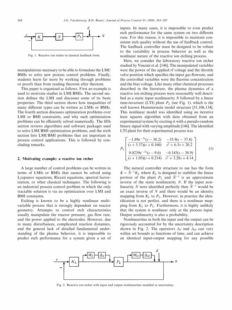
manipulations necessary to be able to formulate the LMI/BMIs to solve new process control problems. Finally,students learn far more by working through problemsor proofs than from reading theorem after theorem.This paper is organized as follows. First an example is

used to motivate studies in LMI/BMIs. The second sec-tion de®nes the LMI and discusses some of its basicproperties. The third section shows how inequalities ofmany di�erent types can be written as LMIs or BMIs.The fourth section discusses optimization problems overLMI or BMI constraints, and why such optimizationproblems can be e�ciently solved numerically. The ®fthsection reviews algorithms and software packages usedto solve LMI/BMI optimization problems, and the sixthsection lists LMI/BMI problems that are important inprocess control applications. This is followed by con-cluding remarks.

2. Motivating example: a reactive ion etcher

A large number of control problems can be written interms of LMIs or BMIs that cannot be solved usingLyapunov equations, Riccati equations, spectral factor-ization, or other classical techniques. The following isan industrial process control problem in which the onlytractable solution is via an optimization over LMI andBMI constaints.Etching is known to be a highly nonlinear multi-

variable process that is strongly dependent on reactorgeometry. Attempts to control etch characteristicsusually manipulate the reactor pressure, gas ¯ow rate,and the power applied to the electrodes. However, dueto many disturbances, complicated reaction dynamics,and the general lack of detailed fundamental under-standing of the plasma behavior, it is impossible topredict etch performance for a system given a set of

inputs. In many cases, it is impossible to even predictetch performance for the same system on two di�erentruns. For this reason, it is impossible to maintain con-sistent etch quality without the use of feedback control.The feedback controller must be designed to be robustto the variability in process behavior as well as thenonlinear nature of the reactive ion etching process.Here, we consider the laboratory reactive ion etcher

studied by Vincent et al. [146]. The manipulated variableswere the power of the applied rf voltage and the throttlevalve position which speci®es the input gas ¯owrate, andthe controlled variables were the ¯uorine concentrationand the bias voltage. Like many other chemical processesdescribed in the literature, the plasma dynamics of areactive ion etching process were reasonably well descri-bed as a static input nonlinearity N followed by a lineartime-invariant (LTI) plant PL (see Fig. 1), which is thewell known Hammerstein model structure [51,106,134].This nonlinear model was identi®ed using an iterativeleast squares algorithm with data obtained from anexperimental system by exciting it with a pseudo-randombinary signal with varying amplitude [146]. The identi®edLTI plant for their experimental process was

PL

ÿ1:89eÿ:5s sÿ 38:2� �s� 5:37� � s� 0:160� �

ÿ35:9 sÿ 37:8� �s2 � 6:5s� 20:2

0:0239eÿ:5s sÿ 9:6� �s� 1:05� � s� 0:214� �

ÿ0:143 sÿ 38:9� �s2 � 3:28s� 4:14

266664377775 �1�

The natural controller structure to use has the formK � Nÿ1KL where KL is designed to stabilize the linearportion of the plant PL and Nÿ1 is an approximateinverse of the static nonlinearity N. If the input non-linearity N were identi®ed perfectly then Nÿ1 would bean exact inverse of N and there would be an identitymapping from KL to PL. However, in practice the iden-ti®cation is not perfect, and there is a nonlinear map-ping from KL to PL. Furthermore, it is highly unlikelythat the system is nonlinear only at the process input.Output nonlinearity is also a probability.Nonlinearities in both the input and the output can be

rigorously accounted for by the uncertainty descriptionshown in Fig. 2. The operators �I and �O can varywithin set bounds as functions of time, and can achievean identical input-output mapping for any possible

Fig. 1. Reactive ion etcher in classical feedback form.

Fig. 2. Reactive ion etcher with input and output nonlinearities modeled as uncertainty.

364 J.G. VanAntwerp, R.D. Braatz / Journal of Process Control 10 (2000) 363±385

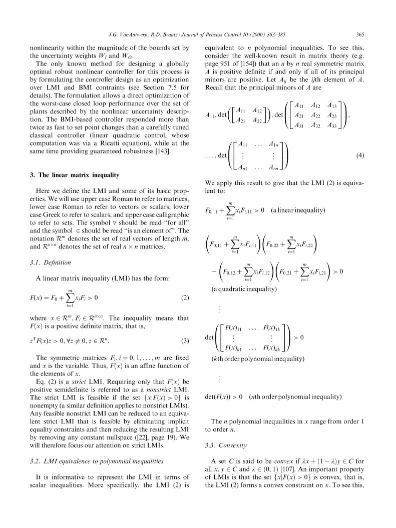
nonlinearity within the magnitude of the bounds set bythe uncertainty weights WI and WO.The only known method for designing a globally

optimal robust nonlinear controller for this process isby formulating the controller design as an optimizationover LMI and BMI contraints (see Section 7.5 fordetails). The formulation allows a direct optimization ofthe worst-case closed loop performance over the set ofplants described by the nonlinear uncertainty descrip-tion. The BMI-based controller responded more thantwice as fast to set point changes than a carefully tunedclassical controller (linear quadratic control, whosecomputation was via a Ricatti equation), while at thesame time providing guaranteed robustness [143].

3. The linear matrix inequality

Here we de®ne the LMI and some of its basic prop-erties. We will use upper case Roman to refer to matrices,lower case Roman to refer to vectors or scalars, lowercase Greek to refer to scalars, and upper case calligraphicto refer to sets. The symbol 8 should be read ``for all''and the symbol 2 should be read ``is an element of''. Thenotation Rm denotes the set of real vectors of length m,and Rn�n denotes the set of real n� n matrices.

3.1. De®nition

A linear matrix inequality (LMI) has the form:

F x� � � F0 �Xmi�1

xiFi > 0 �2�

where x 2 Rm;Fi 2 Rn�n. The inequality means thatF x� � is a positive de®nite matrix, that is,

zTF x� �z > 0; 8z 6� 0; z 2 Rn: �3�

The symmetric matrices Fi; i � 0; 1; . . . ;m are ®xedand x is the variable. Thus, F x� � is an a�ne function ofthe elements of x.Eq. (2) is a strict LMI. Requiring only that F x� � be

positive semide®nite is referred to as a nonstrict LMI.The strict LMI is feasible if the set xjF x� � > 0f g isnonempty (a similar de®nition applies to nonstrict LMIs).Any feasible nonstrict LMI can be reduced to an equiva-lent strict LMI that is feasible by eliminating implicitequality constraints and then reducing the resulting LMIby removing any constant nullspace ([22], page 19). Wewill therefore focus our attention on strict LMIs.

3.2. LMI equivalence to polynomial inequalities

It is informative to represent the LMI in terms ofscalar inequalities. More speci®cally, the LMI (2) is

equivalent to n polynomial inequalities. To see this,consider the well-known result in matrix theory (e.g.page 951 of [154]) that an n by n real symmetric matrixA is positive de®nite if and only if all of its principalminors are positive. Let Aij be the ijth element of A.Recall that the principal minors of A are

A11; detA11 A12

A21 A22

� �� ; det

A11 A12 A13

A21 A22 A23

A31 A32 A33

264375

0B@1CA;

. . . ; det

A11 . . . A1n

..

. ...

An1 . . . Ann

264375

0B@1CA �4�

We apply this result to give that the LMI (2) is equiva-lent to:

F0;11 �Xmi�1

xiFi;11 > 0 �a linear inequality�

F0;11 �Xmi�1

xiFi;11

!F0;22 �

Xmi�1

xiFi;22

!

ÿ F0;12 �Xmi�1

xiFi;12

!F0;21 �

Xmi�1

xiFi;21

!> 0

�a quadratic inequality�

..

.

det

F x� �11 . . . F x� �1k... ..

.

F x� �k1 . . . F x� �kk

264375

0B@1CA > 0

�kth order polynomial inequality�

..

.

det F x� �� > 0 �nth order polynomial inequality�

The n polynomial inequalities in x range from order 1to order n.

3.3. Convexity

A set C is said to be convex if lx� 1ÿ l� �y 2 C forall x; y 2 C and l 2 0; 1� � [107]. An important propertyof LMIs is that the set xjF x� � > 0f g is convex, that is,the LMI (2) forms a convex constraint on x. To see this,

J.G. VanAntwerp, R.D. Braatz / Journal of Process Control 10 (2000) 363±385 365

let x and y be two vectors such that F x� � > 0 andF y� � > 0, and let l 2 0; 1� �. Then

F lx� 1ÿ l� �y� � � F0 �Xmi�1

lxi � 1ÿ l� �yi� �Fi

� lF0 � 1ÿ l� �F0 � lXmi�1

xiFi

� 1ÿ l� �Xmi�1

yiFi

� lF x� � � 1ÿ l� �F y� �

> 0: �5�

3.4. LMIs are not unique

The same set of variables x can be represented as thefeasible set of di�erent LMIs. For instance, if A x� � ispositive de®nite then A x� � subject to a congruencetransformation (see section 14.7 of [154]) is also positivede®nite:

A > 0() xTAx > 0; 8x 6� 0 �6�

() zTMTAMz > 0; 8z 6� 0;M nonsingular �7�

()MTAM > 0 �8�

This implies, for example, that some rearrangementsof matrix elements do not change the feasible set of theLMI.

A B

C D

� �> 0() 0 I

I 0

� �A B

C D

� �0 I

I 0

� �> 0

() D C

B A

� �> 0 �9�

3.5. Multiple LMIs can be expressed as a single LMI

One of the advantages of representing process controlproblems with LMIs is the ability to consider multiplecontrol requirements by appending additional LMIs.Consider a set de®ned by q LMIs:

F1 x� � > 0;F2 x� � > 0; . . . ;Fq x� � > 0 �10�

Then an equivalent single LMI is given by

F x� � � F0 �Xmi�1

xiFi � diag F1 x� �;F2 x� �; . . . ;Fq x� �� > 0;

�11�

where

Fi � diag F1i ;F

2i ; . . . ;Fq

i

� ; 8i � 0; . . . ;m �12�

and diag X1;X2; . . . ;Xq

� is a block diagonal matrix

with blocks X1;X2; . . . ;Xq. This result can be provedfrom the fact that the eigenvalues of a block diagonalmatrix are equal to the union of the eigenvalues of theblocks, or from the de®nition of positive de®niteness.

4. The generality of LMIs and BMIs

This section shows how many common inequalitiescan be written as LMIs. In addition, it shows how manycontrol properties of interest can be written exactly interms of the feasibility of an LMI. Such a problem isreferred to as an LMI feasibility problem.

4.1. Linear constraints can be expressed as an LMI

Linear constraints are ubiquitous in process controlapplications. Model Predictive Control has become themost popular multivariable controller design method inmany industries precisely because of its ability to addresslinear constraints on process variables [32,48,61,95,110,114]. The standard linear programming and quadraticprogramming model predictive control formulationscan be written in terms of LMIs. Here we show the ®rststep, which is to write the linear constraints on processvariables as LMI constraints.Consider the general linear constraint Ax < b written

as n scalar inequalities:

bi ÿXmj�1

Aijxj > 0; i � 1; . . . ; n �13�

where b 2 Rn, A 2 Rn�m, and x 2 Rm. Each of the nscalar inequalities is an LMI. Since multiple LMIs canbe written as a single LMI, the linear inequalities (13)can be expressed as a single LMI.

4.2. Stability of linear systems

Stability is one of the most basic needs for any closedloop system. Some methods for analyzing the stabilityof linear systems are covered in undergraduate processcontrol textbooks [102,133]. Moreover, some nonlinearprocesses can be analyzed (at least to some degree) withlinear techniques by performing a change of variables,such as in binary distillation [91] and pH neutralization[68,101].The Lyapunov method for analyzing stability is

described in most texts on process dynamics [70,108].The basic idea is to search for a positive de®nite func-tion of the state (called the Lyapunov function) whose


time derivative is negative de®nite. A necessary andsu�cient condition for the linear system

x: � Ax �14�

to be stable is the existence of a Lyapunov functionV x� � � xTPx where P is a symmetric positive de®nitematrix such that the time derivative of V is negative forall x 6� 0 [108]:

dV x� �dt� x:TPx� xTPx

:

� xT ATP� PAÿ �

x < 0; 8x 6� 0 �15�

() ATP� PA < 0 �16�

This is an LMI, where P is the variable. To see this,select a basis for symmetric n� n matrices.As an example basis, for i5j de®ne Eij as the matrix

with its i; j� � and j; i� � elements equal to one, and all ofits other elements equal to zero. There are m �n n� 1� �=2 linearly independent matrices Eij and anysymmetric matrix P can be written uniquely as

P �Xnj�1

Xni5j

PijEij; �17�

where Pij is the i; j� � element of P. Thus the matrices Eij

form a basis for symmetric n� n matrices (in fact, if thecolumns of each Eij are stacked up as vectors, then theresulting vectors form an orthogonal basis, which couldbe made orthonormal by scaling).Substituting for P in terms of its basis matrices gives

the alternative form for the Lyapunov inequality

ATP� PA � ATXnj�1

Xni5j

PijEij

!�

Xnj�1

Xni5j

PijEij

!A

�Xnj�1

Xni5j

Pij ATEij � EijA

ÿ �< 0

�18�which is in the form of an LMI (2), with F0 � 0 andFk � ÿATEij ÿ EijA; for k � 1; . . . ;m. The elements ofthe vector x in (2) are the Pij; i5j, stacked up on top ofeach other.

4.3. Stability of nonlinear and time varying systems

Many of the processes commonly encountered inprocess control applications can be adequately modeledas being linear time invariant (LTI). However, manychemical processes cannot be adequately analyzed using

LTI techniques, including reactive ion etching [140],packed bed reactors [46], and most batch processes [9].In Section 4.2, we showed how testing the stability of

a linear system could be posed as an LMI feasibilityproblem. Now let us consider a generalization of thatproblem to testing the stability of a set of linear timevarying systems that are described by a convex hull ofmatrices (a matrix polytope):

x: � A t� �x; A t� � 2 Co A1; . . . ;ALf g �19�

An alternative way of writing this is [105]:

x: � A t� �x; A t� � �

XLi�1

liAi; 8li50;XLi�1

li � 1: �20�

A necessary and su�cient condition for the existenceof a quadratic Lyapunov function V x� � � xTPx thatproves the stability of (20) is the existence of P � PT >0 that satis®es:

dV x� �dt� x:TPx� xTPx

:< 0; 8x 6� 0;

8A t� � 2 Co A1; . . . ;ALf g�21�

() xT A t� �TP� PA t� �� x < 0; 8x 6� 0;

8A t� � 2 Co A1; . . . ;ALf g�22�

() A t� �TP� PA t� � < 0; 8A t� � 2 Co A1; . . . ;ALf g

�23�

()XLi�1

liAi

!T

P� PXLi�1

liAi

!< 0; 8li50;

XLi�1

li � 1

�24�

()XLi�1

li ATi P� PAi

ÿ �< 0; 8li50;

XLi�1

li � 1 �25�

() ATi P� PAi < 0; 8i � 1; . . . ;L �26�

The search for P that satis®es these inequalities is anLMI feasibility problem. This condition is also a su�-cient condition for the stability of nonlinear time vary-ing systems where the Jacobian of the nonlinear systemis contained within the convex hull in (20) [84]. Thereare several di�culties in applying the LMI condition foranalyzing stability of nonlinear systems. First, it is verydi�cult to construct a convex hull for which the Jaco-bian of a nonlinear system is provably contained within.


Second, such a description will usually be highly con-servative, since the convex hull overbounds the Jacobianof the real nonlinear system. Third, each new vertexadds another matrix inequality to the LMI feasibilityproblem (26). For a system with a large number ofstates (which is equal to the dimension of A) and ver-tices (L), solving the LMI feasibility problem (26) canbecome computationally prohibitive. The strength ofthe approach is that LMIs for controller synthesis forsystems of the form (20) are relatively easy to construct[22,77,131].

4.4. The Schur complement lemma

The Schur complement lemma converts a class ofconvex nonlinear inequalities that appears regularly incontrol problems to an LMI. The convex nonlinearinequalities are

R x� � > 0; Q x� � ÿ S x� �R x� �ÿ1S x� �T> 0; �27�

where Q x� � � Q x� �T;R x� � � R x� �T, and S x� � dependa�nely on x. The Schur complement lemma convertsthis set of convex nonlinear inequalities into theequivalent LMI

Q x� � S x� �S x� �T R x� �

� �> 0: �28�

A proof of the Schur complement lemma using onlyelementary calculus is given in the Appendix. In whatfollows, the Schur complement lemma is applied toseveral inequalities that appear in process control.

4.5. Maximum singular value

The maximum singular value measures the maximumgain of a multivariable system, where the magnitude ofthe input and output vector is quanti®ed by the Eucli-dean norm [130]. It is also very useful for quantifyingfrequency-domain performance and robustness formultivariable systems [96,130]. Process applications areprovided in many popular undergraduate process con-trol textbooks [102,126].The maximum singular value of a matrix A which

a�nely depends on x is denoted by � A x� �� , which isthe square root of the largest eigenvalue of A x� �A x� �T.The inequality � A x� �� < 1 is a nonlinear convex con-straint on x that may be written as an LMI using theSchur complement lemma:

� A x� �� < 1() A x� �A x� �T< I �29�() Iÿ A x� �Iÿ1A x� �T> 0 �30�

() I A x� �A x� �T I

� �> 0 �31�

Here A x� � corresponds to S x� � in the LMI (28), andQ x� � and R x� � correspond to I.

4.6. Ellipsoidal inequality

Ellipsoid constraints are important in process identi-®cation, parameter estimation, and statistics [15,27,41,85]; as well as certain fast model predictive controlalgorithms [138,139]. Applications recently described inthe literature include crystallization processes [88,93],polymer ®lm extruders [54], and paper machines [138,139].An ellipsoid described by

xÿ xc� �TPÿ1 xÿ xc� � < 1; P � PT > 0 �32�

can be expressed as an LMI using the Schur comple-ment lemma with Q x� � � 1, R x� � � P, and S x� � �xÿ xc� �T:

1 xÿ xc� �Txÿ xc� � P

� �> 0: �33�

4.7. Algebraic Riccati inequality

Algebraic Riccati equations are used extensively inoptimal control, as described in textbooks on advancedprocess control [111,130], which describe applications tochemical reactors, distillation columns, and other pro-cesses. A result involving a Riccati equation can bereplaced with an equivalent result where the equality isreplaced by an inequality [151]. More speci®cally, theseoptimal controllers can be constructed by computing apositive de®nite symmetric matrix P that satis®es thealgebraic Riccati inequality:

ATP� PA� PBRÿ1BTP�Q < 0 �34�

where A and B are ®xed, Q is a ®xed symmetric matrix,and R is a ®xed symmetric positive de®nite matrix.The Riccati inequality is quadratic in P but can be

expressed as a linear matrix inequality by applying theSchur complement lemma:

ÿATPÿ PAÿQ PBBTP R

� �> 0: �35�

The next two sections provide examples of algebraicRiccati inequalities for analyzing the properties of linearor nonlinear systems.

4.8. Bounded real lemma

The Bounded real lemma forms the basis for LMIapproaches to robust process control which have been


applied to reactive ion etching [140,143], polymerextruders [141], and paper machines [141], and gainscheduling which has been applied to chemical reactors[12,13]. Although the Bounded real lemma has applica-tion to the control of both linear and nonlinear pro-cesses, the actual result is based on the state spacesystem representation of a linear system

x: � Ax� Bu; y � Cx�Du; x 0� � � 0; �36�

where A 2 Rn�n;B 2 Rn�p;C 2 Rp�n, and D 2 Rp�p

are given data. Assume that A is stable and thatA;B;C� � is minimal [74]. The transfer function matrix is

G s� � � C sIÿ A� �ÿ1B�D: �37�

The worst-case performance of a system measured interms of the integral squared errors of the input andoutput is quanti®ed by the H1 norm [157]:

k G s� � k1� supRe s� �>0

� G s� �� sup!2R

�� G j!� �� : �38�

The H1 norm can be written in terms of an LMI. Tosee this, we will use a result from the literature [158] thatthe H1 norm of G s� � is less than if and only if 2IÿDTD > 0 and there exists P � PT > 0 such that

ATP� PA� CTCÿ �� PB� CTD

ÿ �� 2IÿDTDÿ �ÿ1

BTP�DTCÿ �

< 0 �39�

The Schur complement lemma implies that this Ric-cati inequality is equivalent to the existence of P � PT >0 such that the following LMI holds:

ÿ ATP� PA� CTC� � ÿ PB� CTD

� �ÿ BTP�DTC� �

2IÿDTD

" #> 0 �40�

which is equivalent to

ATP� PA� CTC PB� CTD

BTP�DTC DTDÿ 2I

" #< 0: �41�

It is common to incorporate weights on the input uand output y so that the condition of interest is whetherthe H1 norm of W1 s� �G s� �W2 s� � is less than 1. A sys-tem with an H1 norm less than one is said to be strictlybounded real. This condition is checked by testing thefeasibility of the LMI using the state-space matrices forthe product W1 s� �G s� �W2 s� �.

4.9. Positive real lemma

Robustness analysis has been widely applied in theprocess control literature. Examples include distillation

columns [129], packed bed reactors [46] and a reactiveion etching [143]. A property that is regularly exploitedin the development of robustness analysis tools [14,72]for linear systems subject to linear or nonlinear pertur-bations is passivity. The linear system (36) is said to bepassive if��0

u t� �Ty t� �dt50 �42�

for all u and �50. This property is equivalent to theexistence of P � PT > 0 such that [22]

ATP� PA PBÿ CT

BTPÿ C ÿDT ÿD

" #40: �43�

It is instructive to show the connection between thebounded real lemma and the positive real lemma [5],especially since it is often referred to in the robust con-trol literature. A standard result from network theory[10,45,125] is that passivity is equivalent to G s� � in (37)being positive real, that is,

G s� ��G s� �50 8Re sf g > 0 �44�

where G s� �� is the complex conjugate transpose of G s� �.The relationship between bounded real and positive

real is that Iÿ G s� �� I� G s� �� ÿ1 is strictly positive realif and only if G s� � is strictly bounded real. This followsfrom [87]

�� A� � < 1() A�A < I �45�

() I� A�� ÿ1 2Iÿ 2A�A� � I� A� �ÿ1> 0 �46�

() I� A�� ÿ1 Iÿ A�� I� A� � � I� A�� Iÿ A� ��

� I� A� �ÿ1 > 0 �47�

() I� A�� ÿ1 Iÿ A�� Iÿ A� � I� A� �ÿ1> 0 �48�

() Iÿ A� � I� A� �ÿ1� �� Iÿ A� � I� A� �ÿ1> 0 �49�

4.10. The S procedure

The S procedure greatly extends the usefulness ofLMIs by allowing non-LMI conditions that commonlyarise in nonlinear systems analysis to be represented asLMIs (although with some conservatism). This techni-que has been applied to the analysis of pH neutraliza-tion processes [119] and crystallization processes [116].First we will describe the S procedure as it applies to

quadratic functions, and then discuss its application to


quadratic forms. Let �0; . . . ; �p be quadratic scalarfunctions of x 2 Rn:

�i x� � � xTTix� 2uTi x� �i; i � 0; . . . ; p; Ti � TTi

�50�The existence of �150; . . . ; �p50 such that

�0 x� � ÿXpi�1�i�i x� �50; 8x; �51�

implies that

�0 x� �50; 8x such that �i x� �50; i � 1; . . . ; p: �52�

To see why this is true, assume there exists�150; . . . ; �p50 such that (51) holds for all�i x� �50; i � 1; . . . ; p. Then

�0 x� �5Xpi�1�i�i x� �50; 8x: �53�

Note that (51) is equivalent to

T0 u0uT0 �0

� �ÿXpi�1�i

Ti uiuTi �i

� �50 �54�

since

xTTx� 2uTx� �50; 8x �55�

() x1

� �TT uuT �

� �x1

� �50; 8x �56�

() �x�

� �TT uuT �

� ��x�

� �50; 8x; � �57�

() T uuT �

� �50: �58�

Hence the above S procedure can be equivalentlywritten in terms of quadratic forms. Instead of writingthe above version which is completely in terms of non-strict inequalities, we will provide here a version thatapplies to the case where the main inequality is strict(the proof is similar). Let T0; . . . ;Tp be symmetricmatrices. If there exists �150; . . . ; �p50 such that

T0 ÿXpi�1�iTi > 0; �59�

then

xTT0x > 08x 6� 0 such that xTTix50; i � 1; . . . ; p: �60�

4.11. Stability of linear systems with nonlinearperturbations

The derivation of LMI feasibility problems to analyzethe stability or performance of linear systems subject tolinear/nonlinear time invariant/varying perturbations israther straightforward conceptually [22], although thealgebra can be messy for more complex systems[115,118]. For continuous time systems, the basicapproach is to postulate a positive de®nite Lyapunovfunction of the state and some undetermined matrices,and then apply the S procedure (if necessary) to deriveLMI conditions on the undetermined matrices whichimply that the time derivative of the Lyapunov functionis negative de®nite. For discrete time systems, the divi-ded di�erence of the Lyapunov function is used insteadof the time derivative. Here we show how this approachis applied to a system of especial relevance to processcontrol applications.Consider a discrete time system subject to slope-

restricted static nonlinearities:

x k� 1� � � Ax k� � � B� q k� �� q k� � � Cx k� � �61�

with the nonlinearities described by

�i qi k� �� i qi k� �� ÿ qi k� �� 40; for i � 1; . . . ;m �62�

with the local slope restrictions

0 <�i qi k� 1� �� ÿ �i qi k� ��

qi k� 1� � ÿ qi k� � < Tii; for i � 1; . . . ;m �63�

where Tii is the maximum slope of the ith nonlinearity.This can be used to represent a linear process withactuator limitation nonlinearities which is controlled byan antiwindup compensator [36,78,30], or a closed loopsystem with each component being either a linear sys-tem or a dynamic arti®cial neural network [117,120].Both of these types of closed loop systems have beenextensively studied in the process control literature (seethe above references and citations therein).The Lur'e-Lyapunov function is de®ned by

V x k� �� xT k� �Px k� � � 2Xmi�1

�qi k� �0

�i �� Qiid� �64�

where P is positive de®nite and the Qii are nonnegativeso that the Lyapunov function is positive de®nite. The®rst term is the standard quadratic Lyapunov functionwhich is discussed in many state space systems text-books [100] and in textbooks on process analysis[70,108], which describe applications to polymerizationand other chemical reactors. The second term was


introduced by Lur'e [86] to include the nonlinearities(62) explicitly in the Lyapunov function.The method of Lyapunov for discrete time systems is

to write the divided di�erence for the Lyapunov function:

V x k� 1� �� ÿ V x k� �� 65�

with the state vector substituted in using (61). Theoverall system is globally asymptotically stable if theundetermined matrices P and Qii can be computed sothat V x k� 1� �� ÿ V x k� �� is less than zero. The non-linearities are bounded in the divided di�erence using(63) and the mean value theorem, and the S procedure isused to convert the divided di�erence subject to theinequalities (62) to an LMI. With some algebra to col-lect the terms [115,118], it is found that a su�cient con-dition for the global asymptotic stability of (61)±(63) isthe existence of a positive-de®nite matrix P and diag-onal positive semide®nite matrices Q and R 2 Rh�h suchthat

M1;1 M1;2

M2;1 M2;2

� �> 0 �66�

where

M1;1 � ÿATPA� Pÿ Aÿ I� �TCTTQC Aÿ I� � �67�

M1;2 � ÿATPBÿ Aÿ I� �TCTTQCB

ÿ Aÿ I� �TCTQÿ CTR �68�

M2;1 � ÿBTPAÿ BTCTTQC Aÿ I� � ÿQC Aÿ I� � ÿ RC

�69�

M2;2 � ÿBTPBÿ BTCTTQCBÿQCBÿ BTCTQ� 2R

�70�

and T � diag Tiif g. The new matrix R is introduced bythe S procedure. This is an LMI feasibility problem thathas been applied to the analysis of pH neutralizationprocesses [119] and crystallization processes [116] undernonlinear feedback control.

4.12. Variable reduction lemma

The variable reduction lemma allows the solution ofalgebraic Riccati inequalities that involve a matrix ofunknown dimension. This often arises when ®nding thecontroller that minimizes the H1 norm (see Section 7.5for an example).Given a symmetric matrix A 2 Rn�n and two matrices

P and Q of column dimension n, consider the problem

of ®nding some matrix � of compatible dimensionssuch that

A� PT�TQ�QT�P < 0 �71�

This equation is solvable for some � if and only if thefollowing two conditions hold:

WTPAWP < 0 �72�

WTQAWQ < 0 �73�

where WP and WQ are matrices whose columns arebases for the null spaces of P and Q, respectively. Aproof of this result is given in [58].

4.13. Bilinear matrix inequality

Bilinear inequalities arise in pooling and blendingproblems [147], systems analysis [140], and nonlinearprogramming. A bilinear matrix inequality (BMI) is ofthe form:

F x; y� � � F0 �Xmi�1

xiFi �Xnj�1

yjGj �Xmi�1

Xnj�1

xiyjHij > 0

�74�

where Gj and Hij are symmetric matrices of the samedimension as Fi, and y 2 Rn. Bilinear matrix inequal-ities were popularized by Safonov and co-workers in aseries of proceedings papers [63±65,125], and ®rstapplied to a nontrivial process description (i.e., a che-mical reactive ion etcher) by VanAntwerp and Braatz[140], and was later applied to paper machines [141].A BMI is an LMI in x for ®xed y and an LMI in y for

®xed x, and so is convex in x and convex in y. Thebilinear terms make the set not jointly convex in x and y.To see this, consider the simplest BMI which is thebilinear inequality

1ÿ xy > 0; �75�

where x and y are scalar variables. One way to see thatthis set is nonconvex is to graph the set in the xy-planeand apply the de®nition of convexity. Another way tosee this is to consider two elements of the set that con-tradict the de®nition of convexity. For example, con-sider x; y� � equal to the values 0:1; 7:9� � and 7:9; 0:1� �.Both values satisfy the bilinear inequality since1ÿ 0:1� � 7:9� � � 1ÿ 7:9� � 0:1� � � 0:21 > 0. But the pointon the line half way between the two values1=2�0:1; 7:9� � 1=2 7:9; 0:1� � � 4; 4� �� does not satisfythe bilinear inequality: 1ÿ 4�4 � ÿ15 < 0.Besides bilinear and general quadratic inequalities

xTQx� cTx� p > 0; �76�


general polynomial inequalities can also be written asBMIs. Consider, for example, the nonlinear inequality

x3 � yz < 1 �77�

By de®ning x2 � w, and x � v, this inequality isequivalent to:

1ÿ xwÿ yz > 0 �78�xÿ v50

vÿ x50

wÿ vx50

vxÿ w50

Since a BMI describes sets that are not necessarilyconvex, they can describe much wider classes of con-straint sets than LMIs, and can be used to representmore types of optimization and control problems. Themain drawback of BMIs is that they are much moredi�cult to handle computationally than LMIs.

5. Optimization problems

Many optimization and control problems can bewritten in terms of ®nding a feasible solution to a set ofLMIs or BMIs. Most problems, however, are best writ-ten in terms of optimizing a simple objective functionover a set of LMIs or BMIs. There is a fundamentaldi�erence between the computational requirements foroptimization problems over LMIs, and those overBMIs. This section begins with an introduction to con-vex optimization and computational complexity, whichprovides a fundamental framework for understandingthe relative complexities of optimization problems. Thisis followed by the de®nition of some optimization pro-blems that appear when formulating and solving controlproblems using LMIs/BMIs.

5.1. Computational complexity and convexity

Optimization problems are generally characterized asbeing in one of two classes: P and NP-hard [62,104]. Theclass P refers to problems in which the time needed toexactly solve the problem can always be bounded by asingle function which is polynomial in the amount ofdata needed to de®ne the problem. Such problems aresaid to be solvable in polynomial time. Although theexact consequences of a problem being NP-hard is still afundamental open question in the theory of computa-tional complexity, it is generally accepted that a pro-blem being NP-hard means that its solution cannot becomputed in polynomial time in the worst case. It is

important to understand that being NP-hard is a propertyof the problem itself, not of any particular algorithm. Itis also important to understand that having a problembe NP-hard does not imply that practical algorithms arenot possible. Practical algorithms for NP-hard problemsexist and typically involve approximation, heuristics,branch-and-bound, or local search [35,62,104]. Deter-mining whether a problem is polynomial time or NP-hard informs the systems engineer what kind of accu-racy and speed can be expected by the best algorithms,and what kinds of algorithms to investigate for provid-ing practical solutions to the problem.Suppose that a real valued function f x� � is de®ned on

a convex set C 2 Rn. The function f x� � is convex on C if[107]

f lx� 1ÿ l� �y� �4lf x� � � 1ÿ l� �f y� � �79�

for all x; y 2 C and l 2 0; 1� �. A convex optimizationproblem has the form

infx2C

f x� �; �80�

where f x� � is a convex function in x, C is a convex set,and inf refers to the in®mum over C. If the in®mum isachieved by an element in C, then the minimizationproblem will be written as min.Well known problems that can be formulated as con-

vex optimization problems include linear programmingand convex quadratic programming. The advantage offormulating control problems in terms of convex opti-mization problems (when possible) is that wide classesof convex optimization problems are in the class P [97].Being in P means that these problems can be provablysolved e�ciently on a computer. This makes convexoptimization problems desirable for solving large scalesystems problems. Convex optimization problems oftenoccur in engineering practice and many can be writtenas LMIs. This is the strength of using LMI formula-tions. Convex optimizations over LMIs are solvable inpolynomial time.Other systems engineering problems cannot be written

in terms of LMIs, but can be written in terms of BMIs.Nearly every control problem of interest can be writtenin terms of an optimization problems over BMIs. Theseoptimization problems, however, are NP-hard [135],which implies that it is highly unlikely that there exists apolynomial-time algorithm for solving these problems.This means that algorithms for solving optimizationproblems over BMIs are currently limited to problemsof modest size. Algorithms and their expected perfor-mance will be discussed in more detail in Section 6. Forthe rest of this section we review the most common LMIand BMI optimization problems that appear in controlapplications.


5.2. Semide®nite programming

The following optimization problem is commonlyreferred to as a semide®nite program (SDP) [4]:

infx

F x� �>0cTx �81�

One SDP which often arises in control applications isthe LMI eigenvalue problem (EVP). It is the minimiza-tion of the maximum eigenvalue of a matrix thatdepends a�nely on the variable x, subject to an LMIconstraint on x. Many performance analysis tests, suchas computing the H1 norm in (38), can be written interms of an EVP [144]. Two common forms of the EVPare presented so that readers will recognize them:

infx;l

lIÿA x� �>0B x� �>0

l �82�

infx;l

A x;l� �>0

l �83�

where A x; l� � is a�ne in x and l.The equivalence of (81), (82), and (83) will now be

demonstrated. The LMI eigenvalue problem (82) can bewritten in the form (83) by de®ning A x; l� � �diag lIÿ A x� �;B x� �f g (recall that multiple LMIs can bewritten as a single LMI of larger dimension). To showthat a problem in the form (83) can be written in theform (81), de®ne x � xT l� �T, F x� � � A x� �, and cT �0T1� �T where 0 is a vector of zeros. To see that (81)transforms to (82) consider

infF x� �>0

cTx � infcTx<lF x� �>0

l � inf1lÿcTx>0F x� �>0

l � inflIÿA x� �>0F x� �>0

l: �84�

QED.

5.3. Generalized eigenvalue problems

A large number of the control properties can becomputed as a generalized eigenvalue problem (GEVP),including many robustness margins and the minimizedcondition number discussed in Section 7. A GEVP is,given square matrices A and B, B > 0, to ®nd scalars land nonzero vectors y such that

Ay � lBy �85�

The computation of the largest generalized eigenvaluecan be written in terms of an optimization problem withLMI-like constraints. Consider that the positive de®-niteness of B implies that for su�ciently large l,

lBÿ A > 0. As l is reduced from some su�ciently highvalue, at some point the matrix lBÿ A will lose rank, atwhich point there exists a nonzero vector y that solves(85), implying that this value of l is the largest general-ized eigenvalue. Hence

lmax � minlBÿA50

l � inflBÿA>0

l �86�

Often it is desired to minimize the largest generalizedeigenvalue of two symmetric matrices which dependa�nely on a variable x, subject to an LMI constraint onx.

infB x� �>0C x� �>0

lmax A x� �;B x� �� : �87�

Here lmax A x� �;B x� �� is the largest generalized eigen-value of two matrices, A and B, each of which dependa�nely on x. From (86) this optimization problem isequivalent to

inflB x� �ÿA x� �>0

B x� �>0C x� �>0

l: �88�

The problem of minimizing the maximum generalizedeigenvalue is a quasiconvex objective function subject toa convex constraint, where quasiconvexity means that

lmax A �x� 1ÿ �� z� �;B �x� 1ÿ �� z� �� 4max lmax A x� �;B x� �� ; lmax A z� �;B z� �� 89�

for all � 2 0; 1� � and all feasible x and z. To see that thisis true, ®rst de®ne l equal to the right hand side of (89).Then

l5lmax A x� �;B x� �� and l5lmax A z� �;B z� �� : �90�

From (86), this implies that

lB x� � ÿ A x� �50 and lB z� � ÿ A z� �50: �91�

It follows that, for all � 2 0; 1� �,

� lB x� � ÿ A x� �h i

� 1ÿ �� lB z� � ÿ A z� �h i

50 �92�

() lB �x� 1ÿ �� z� � ÿ A �x� 1ÿ �� z� �50: �93�

This and (86) imply that

l5lmax A �x� 1ÿ �� z� �;B �x� 1ÿ �� z� �� : �94�

QED.


5.4. Convex determinant optimization problem

We will refer to the following as a convex determinantoptimization problem (CDOP):

infA x� �>0B x� �>0

log det A x� �ÿ1ÿ � �95�

where A and B are symmetric matrices which are a�nefunctions of x. As we will see in Section 7, this problemappears in a variety of ellipsoidal approximation pro-blems associated with state and parameter estimationproblems, and in optimal experimental design. Theproof that log det A x� �ÿ1

� �� ÿ log det A� �� is con-

vex, which implies that a CDOP can be solved relativelye�ciently on a computer, is given in the appendix.

5.5. BMI problem

An optimization over BMI constraints is called a BMIproblem:

infx;y

A xTyT� �T� �>0F x;y� �>0

cTx� dTy �96�

where F x; y� � is de®ned in (74).Many important problems in control that cannot be

stated in terms of LMIs can be stated in terms of BMIs.Examples include robustness analysis [43,109], a largenumber of robust controller synthesis problems includ-ing low order and decentralized control [125,63], bilin-ear programming, and linear complementarity problems[2,3,42]. Additionally, a large number of process designproblems can be written exactly or approximately in thisform [124,147,148].In the same way that the EVP (82) is an optimization

over LMI constraints, there is a corresponding optimi-zation over BMI constraints called the BMI eigenvalueproblem (BEVP):

infx;y;

A xTyT� �T� �>0lmax F x;y� �� <

�97�

where lmax is the maximum eigenvalue of F x; y� �.Using algebra similar as for the LMI eigenvalue pro-

blem, it can be shown that this is a special case of theBMI optimization problem.

6. Solving optimizations over LMI or BMI constraints

Here we outline the algorithms and review softwareused to solve optimization problems over LMIs andBMIs.

6.1. Solving LMI problems

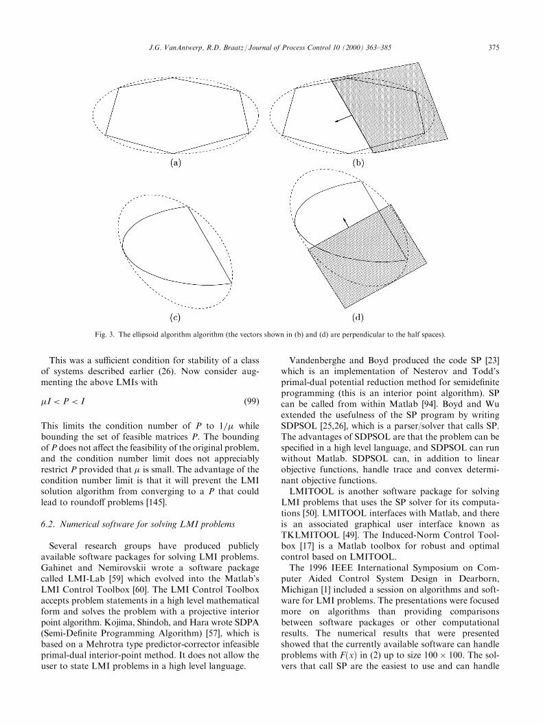
The easiest algorithm to implement for solving LMIproblems is the ellipsoid algorithm (see Fig. 3) [18]. Itsolves a convex objective function with convex con-straints. In the ®rst step, an ellipsoid is computed thatcontains the optimum point. Often this means comput-ing an ellipsoid that covers the constraint set (see Fig.3a). The next step is to compute a plane that passesthrough the center of the ellipsoid such that the solutionis guaranteed to lie on one side of the plane (Fig. 3b).Boyd et al. [22] gives analytical expressions for this cut-ting plane for each of the LMI problems. The mainpoint is that for each of the LMI problems there is ahalf space which is de®nitely ``uphill,'' so that any pointsin that half space can be discarded. The remaining halfellipsoid is itself covered by an ellipsoid of minimalvolume (Fig. 3c) and the process is repeated (Fig. 3d)until the algorithm converges to the optimal solution.A more computationally e�cient algorithm for sol-

ving LMI problems is the interior point method [97].The interior point method uses the constraints to de®nea barrier function which is convex within the feasibleregion and in®nite outside it. This barrier function isincorporated into an objective function, which allowsthe constrained optimization problem to be replacedwith an unconstrained optimization problem which canbe solved using Newton's method. The analytic center isde®ned to be the point which minimizes the uncon-strained optimization problem. A scalar in the objectiveto the unconstrained optimization problem is iterateduntil the analytic center is optimal for the original problem.The interior point method is, in some ways, similar to

the penalty function method [107]. In both cases, theconstraint set is incorporated into the objective functionof an unconstrained optimization problem which can besolved using Newton's method. Also, in both cases ascalar in the objective is iterated until the solution to theunconstrained optimization problem is equal to thesolution to the original problem. However, both theobjective functions and the scalar that is iterated are dif-ferent in the two methods. The ellipsoid algorithm, onthe other hand, works more like a standard branch andbound algorithm [90], in that it is continually discardinginfeasible regions from the search. For an optimizationover a single scalar variable, the ellipsoid algorithm isequivalent to the bisection algorithm [44].A modi®cation to the LMIs that can be critical for

obtaining convergence of these algorithms is to includea constraint that keeps the numerics well conditionedand the variables bounded. It is simplest to illustratethis modi®cation with an example. Consider, for exam-ple, the search for a P � PT > 0 that satis®es the LMIfeasibility problem

ATi P� PAi < 0; 8i � 1; . . . ;L �98�


This was a su�cient condition for stability of a classof systems described earlier (26). Now consider aug-menting the above LMIs with

�I < P < I �99�

This limits the condition number of P to 1=� whilebounding the set of feasible matrices P. The boundingof P does not a�ect the feasibility of the original problem,and the condition number limit does not appreciablyrestrict P provided that � is small. The advantage of thecondition number limit is that it will prevent the LMIsolution algorithm from converging to a P that couldlead to roundo� problems [145].

6.2. Numerical software for solving LMI problems

Several research groups have produced publiclyavailable software packages for solving LMI problems.Gahinet and Nemirovskii wrote a software packagecalled LMI-Lab [59] which evolved into the Matlab'sLMI Control Toolbox [60]. The LMI Control Toolboxaccepts problem statements in a high level mathematicalform and solves the problem with a projective interiorpoint algorithm. Kojima, Shindoh, and Hara wrote SDPA(Semi-De®nite Programming Algorithm) [57], which isbased on a Mehrotra type predictor-corrector infeasibleprimal-dual interior-point method. It does not allow theuser to state LMI problems in a high level language.

Vandenberghe and Boyd produced the code SP [23]which is an implementation of Nesterov and Todd'sprimal-dual potential reduction method for semide®niteprogramming (this is an interior point algorithm). SPcan be called from within Matlab [94]. Boyd and Wuextended the usefulness of the SP program by writingSDPSOL [25,26], which is a parser/solver that calls SP.The advantages of SDPSOL are that the problem can bespeci®ed in a high level language, and SDPSOL can runwithout Matlab. SDPSOL can, in addition to linearobjective functions, handle trace and convex determi-nant objective functions.LMITOOL is another software package for solving

LMI problems that uses the SP solver for its computa-tions [50]. LMITOOL interfaces with Matlab, and thereis an associated graphical user interface known asTKLMITOOL [49]. The Induced-Norm Control Tool-box [17] is a Matlab toolbox for robust and optimalcontrol based on LMITOOL.The 1996 IEEE International Symposium on Com-

puter Aided Control System Design in Dearborn,Michigan [1] included a session on algorithms and soft-ware for LMI problems. The presentations were focusedmore on algorithms than providing comparisonsbetween software packages or other computationalresults. The numerical results that were presentedshowed that the currently available software can handleproblems with F x� � in (2) up to size 100� 100. The sol-vers that call SP are the easiest to use and can handle

Fig. 3. The ellipsoid algorithm algorithm (the vectors shown in (b) and (d) are perpendicular to the half spaces).


bigger problems than the other software. As of thepublication of this tutorial, none of the above LMI sol-vers exploit matrix sparsity to a high degree.

6.3. Solving BMI problems

Consider the following BMI problem, where we havede®ned l and r as those variables which appear in theBMI constraint:

infA l;r;x;y; � �>0

F0�Pi

Pj

li;rjFij>0

li4li4li

rj4rj4rj

�100�

where A is jointly a�ne in l, r, x, y, and .A global optimization approach such as branch and

bound is required for guaranteed convergence to the globaloptimum of a BMI problem because the BMI problemis not convex. While several branch and bound algo-rithms have been developed for solving BMI problems[64,155,156], what appears to be the most e�cient algo-rithm was developed relatively recently [136,140,141,142,143]. The art to developing an e�cient branch andbound algorithm is to derive tight upper and lowerbounds for the objective function over any given part ofthe domain. Reducing the ranges of all problem vari-ables as much as possible is frequently the key to tightobjective function bounding. The approach uses LMIrelaxations as lower bounds for the BMI.


F0�Pi

Pj

li;rjFij>0

l�i4li4l

�i

r�j4rj4r�j

� infA l;r;x;y; � �>0

F0�Pi

Pj

wijFij>0

l�i4li4l

�i

r�j4rj4r�jwij�lirj

5 infA l;r;x;y; � �>0

F0�Pi

Pj

wijFij>0

l�i4li4l�i

r�i4ri4r�i

wij2 w�ij;w� ij

h i

�101�

where the overbar (underbar) indicates the upper(lower) bound for a variable and

w�ij � min l

�ir�j; l�ir

�j; l

�ir�j; l�ir�j

n o�102�

w� ij � max l�ir�j; l�ir

�j; l

�ir�j; l�ir�j

n o: �103�

Further, because wij is a bilinear term the followingadditional constraints may be included in the lowerbound (101) [90]:

wij4r�jli � l�irj ÿ r

�jl�i

wij4l�irj � r�jli ÿ l

�ir�j

wij5l�irj � r�jli ÿ r�jl�iwij5l

�irj � r

�jli ÿ l

�ir�j

: �104�

An LMI upper bound is derived by local optimizationor by ®xing some of the variables. For instance:


l�i4li4l�i

r�j4rj4r�j

F0�Pi

Pj

lirjFij>0

4 infA l;r;x;y; � �>0

li�l�i

r�j4rj4r�j

F0�Pi

Pj

lirjFij>0

�105�

With these polynomial-time computable LMI upperand lower bounds, the nonconvex optimization (100) isideal for the application of the branch and bound algo-rithm. Interested readers are referred to [137] for moredetails.

7. Applications

This section lists a variety of LMI and BMI problemsthat have been or should be studied in process control.

7.1. Control structure selection

Assume that the matrix M 2 Rn�m; n5m is full rank.The condition number of M is the ratio of its largestsingular value to its smallest

� M� � � �� M� ��M� � : �106�

The condition number appears rather naturally inmany control problems, including control structureselection [121,96,102,130,149] and model identi®cation[121,54,83]. It is certainly the one of the most used (andmisused [82,28,29]) matrix functions in process control.Its application to chemical processes such as distillationcolumns is described in many undergraduate processcontrol textbooks [102,126].Another matrix function that is more relevant to many

applications is the minimized condition number:

infR;L

� LMR� � �107�

where L 2 Rn�n and R 2 Rm�m are diagonal and non-singular. The minimized condition number (107) is usedfor integral controllability tests based on steady-stateinformation [67,96] and for the selection of sensors andactuators using dynamic information [38,112,38,99,98].The sensitivity of stability to uncertainty in control sys-tems is given in terms of the minimized condition num-ber in [127,128]. The minimized condition number isapplied regularly in the process industries, as part of theRobust Multivariable Predictive Control Technologysold by Honeywell [89]. The application to a fractio-nator and a paper machine is described in [89].


It was shown in [30] how to pose the minimized con-dition number as a GEVP (88). Here we provide analternative derivation that follows the later derivation in[22]. Note that the de®nition of the condition numberimplies that it is greater than or equal to 1. For 51, wehave that

� LMR� �4 () �I4 LMR� �T LMR� �4� 2I �108�

() I4 LMR� �T

LMR� �

4 2I �109�

() RRTÿ �ÿ1

4MT LTL� �

M4 2 RRTÿ �ÿ1 �110�

() Q4MTPM4 2Q �111�

for diagonal P > 0 2 Rn�n and diagonal Q > 0 2 Rm�m.Therefore, solving the minimized condition numberproblem (107) is equivalent to solving the GEVP (88):

infP>0Q>0

Q4MTPM4 2Q

2 �112�

where P and Q are diagonal.

7.2. Parameter estimation and model predictive control

The approximation of polytopes with ellipsoids havenumerous applications, including parameter estimation[39,56,80] and model predictive control [34,138,139].The model predictive control application has beenimplemented on paper machine models constructedfrom industrial data [139].An ellipsoid has the form

" � By� dj k y k41� �113�

where B � BT > 0. This ellipsoid is centered at d andhas volume proportional to det B� �. Consider the poly-tope

P � xjATi x4bi; i � 1; . . . ;L

� �114�

where ATi is the ith row of the matrix A. An ellipsoid E is

contained inside the polytope P if

ATi By� d� �4bi8y; k y k41 �115�

() maxkyk41

ATi By� AT

i d4bi �116�

() k BAi k �ATi d4bi �117�

Thus, the maximum volume ellipsoid E contained inthe polytope P is given by

maxB�BT>0;d

kBAik�ATid4bi

log det B� � �118�

This optimization is convex in the variables B and d.For the case where the center of the ellipsoid is known(e.g. d � 0 when Ax4b de®nes a symmetric polytope),(117) can be written as an LMI using the Schur com-plement lemma:

k BAi k �ATi d4bi () bi ÿ AT

i d50 and

k BAi k2 4 bi ÿ ATi d

ÿ �2 �119�

() bi ÿ ATi d50 and bi ÿ AT

i dÿ �2ÿAT

i BIÿ1BAi50

�120�

() bi ÿ ATi d

ÿ �2AT

i BBAi I

� �50; 8i 2 1;L� � �121�

Hence in this case (118) can be written as the CDOP(95):

maxB�BT>0;d

biÿATi d� �2 AT

i B

BAi I

� �50

log det B� � �122�

In the case where d is unknown, (118) is not an LMIbut is still a convex program that can be solved, forinstance, by interior point methods [76,97].A related problem of interest is to determine the

smallest ellipsoid which encloses a given polytope. Firstde®ne the convex hull of a given set of points T in Rn asthe set of all convex combinations of points in T . Anequivalent de®nition is the smallest convex set contain-ing T [105]. Let the polytope be described as the convexhull of its vertices

P � Co v1; . . . ; vLf g �123�

and write the ellipsoid

E � xj k Axÿ b k41;A � AT > 0�

; �124�

where its center is Aÿ1b and its volume is proportionalto det Aÿ1

ÿ �. Then the minimum volume ellipsoid which

encloses the polytope is given by

infA�AT>0kAviÿbk41

log det Aÿ1ÿ �

: �125�


This problem is convex in A and b, and can be writtenas a CDOP (95) by applying the results of Section 4.6:

infA�AT>0

1 Aviÿb� �TAviÿb I

� �>0

log det Aÿ1ÿ � �126�

7.3. Optimal design of experiments

The goal of optimal experimental design is to max-imize the informativeness of data collected from theprocess [11]. Optimal experimental design algorithmshave been applied to chemical kinetics [20,19,21,73,113],synthetic ®ber manufacture [75], petroleum fractiona-tion [132], crystallization [92], distillation [79], andpolymer ®lm extrusion [53]. While most formulationsrequire the solution of nonconvex optimization pro-blems [69,150], here is presented a formulation for linearparameter estimation which requires only the solutionof a CDOP (95).The goal is to estimate a vector of parameters x from

some measurement y � Ax� w where A is a matrix ofinputs and w is zero-mean white measurement noise.The error covariance of the minimum variance esti-mator is ATA� �ÿ1. If the rows of A � a1; . . . ; aL� �T arechosen from a set of possible test vectors,

ai 2 v1; . . . ; vLf g; i � 1; . . . ;L; �127�the goal of D-optimal experimental design is to selectthe vectors so that the determinant of the error covar-iance is minimized.We can write

ATA �XLi�1

livivTi �128�

where li50 is the fraction of rows equal to the vector vi,which implies that

PLi�1li � 1. When L is a large num-

ber, the li can be treated as continuous variables insteadof integer multiples of 1/L.Then the D-optimal design problem is the CDOP (95)

[153]:

infli50PL

i�1li�1

log detXLi�1

livivTi

!ÿ1�129�

7.4. Robust control system analysis

The robustness margin for a variety of linear systemssubject to linear or nonlinear perturbations[31,71,96,123,130] can be computed by solving

� � infD2D

�� DMDÿ1ÿ � �130�

where M is a complex matrix and D is the set of com-plex nonsingular block diagonal matrices with someblocks possibly being repeated. This robustness marginhas been applied to numerous processes over the past 15years, including distillation columns [29,40,96,130], pHneutralization [119], packed bed reactors [47], papermachines [81,122,33], polymer ®lm extrusion [52,55],and reactive ion etching [143].This problem can be written in terms of a GEVP (88):

�2 � infD2D

DMDÿ1� �� DMDÿ1� �4 2I

2 �131�

� infD2D

M�D�DM4 2D�D

2 �132�

� infP2P

M�PM4 2P

2 �133�

where P is the set of complex symmetric positive de®niten� n block diagonal matrices with the correspondingblocks from D being repeated.

7.5. Robust nonlinear controller synthesis

BMI formulations arise naturally in the design ofrobust optimal inversion-based controllers for nonlinearprocesses. Here we present the BMI formulation which wasapplied to the nonlinear simulation model of a reactiveion etcher constructed from experimental data presentedin Section 2. The BMI-based controller demonstratedsubstantially improved performance and robustnessover a traditional nonlinear controller [140,143].After the nonlinear inversion technique removed the

most signi®cant nonlinearities, the control synthesisproblem consisted of designing a linear controller for alinear plant subject to norm-bounded nonlinear timevarying perturbations. The state space realization forthe plant transfer function G s� � � C sIÿ A� �ÿ1B�Dwas represented by

G �A B1 B2

C1 D11 D12

C2 D21 D22

24 35 �134�

where D22 � 0 without loss of generality [157]. Thecontroller that optimizes the induced 2-norm perfor-mance objective subject to the constraint of stability ofthe closed loop system with norm-bounded nonlineartime varying perturbations was computed from thesolution of the BEVP (97) [140,143]:

� � infL;R;X;Y� �2B

lmax L1R1� �41

�135�


where B is the set such that L, R, X and Y are symmetricmatrices,

L � L1 00 I

� �; R � R1 0

0 I

� �; L1;R1 2 D; �136�

and

B2

D12

� �?0

0 I

264375 AX� XAT XCT

1 B1

C1X ÿL D11

BT1 DT

11 ÿR

24 35

�B2

D12

� �?T

0

0 I

26643775< 0; �137�

CT2

DT21

!?0

0 I

2666437775 YA� ATY YB1 CT

1

BT1Y ÿR D11

C1 DT11 ÿL

24 35

�CT

2

DT21

!?T

0

0 I

2666437775< 0; �138�

X II Y

� �> 0: �139�

Here A? is a matrix whose rows form a basis for thenull space of AT. The only nonconvexity in (135) is theconstraint lmax L1R1� �41 (which is a BMI).As the algebra of this derivation is lengthy and

involved, only a summary is given here. The state spaceequations for the closed loop system are written asfunctions of the state space matrices of the plant and thecontroller. A version of the Bounded real lemma is usedto write the induced 2-norm performance objective interms of matrix inequalities, and the variable reductionlemma of Section 4.12 is used to remove explicit depen-dence of the matrix inequalities on the controller statespace matrices. Finally, D and Dÿ1 are replaced with Land R and the additional constraint that lmax R1L1� �< 1. Readers interested in a detailed derivation arereferred to [137].A closely related formulation was used in the design

of linear controllers that optimize the robust perfor-mance for large scale sheet and ®lm processes, such aspolymer ®lm extruders and paper machines [141]. Inthose particular applications, the only process non-linearities were perturbations about the nominal lineardynamics.

7.6. Robust model predictive control

Here we describe an LMI-based robust model pre-dictive control algorithm which applied to a non-isothermal nonadiabatic continuous stirred tank reactor(CSTR) [77]. The LMI approach provided similar per-formance as a non-LMI-based model predictive controlalgorithm, while having the capability of providingrobustness to model uncertainty.Consider the discrete time time varying linear system

x k� 1� � � A k� �x k� � � B k� �u k� � �140�

y k� � � C k� �x k� � �141�

where each state space matrix is arbitrarily time varyingand lies within a polytope (see Section 4.3). De®nex kjk� � as the state of the uncertain system measured atsampling time k, x k� ijk� � as the state of the system attime k� i predicted at time k, u k� ijk� � as the controlmove at time k� i computed at time k, and W and Rare positive de®nite weighting matrices. For this controlproblem, the objective was to compute the state feed-back matrix F:

u k� ijk� � � Fx k� ijk� � �142�

so as to minimize an upper bound on the in®nite hor-izon quadratic objective:X1i�0

x k� ijk� �TWx k� ijk� � � u k� ijk� �Ru k� ijk� �: �143�

at sampling time k. This state feedback matrix is givenby [77]:

F � YQÿ1 �144�

where Q > 0 and Y are solutions to the following EVP(82):

inf ;Q;Y

�145�

subject to

1 x kjk� �Tx kjk� � Q

� �50 �146�

Q QATi � YTBT

i QW1=2 YTR1=2

AiQ� BiY Q 0 0W1=2Q 0 I 0R1=2Y 0 0 I

2664377550;

8i � 1; 2; . . . ;L:

�147�


The derivation uses a positive de®nite quadraticfunction of the state to bound the performance objective(143), and then uses the Schur complement lemma tomanipulate this inequality into the form of the LMIconstraint (147). Input and output constraints can alsobe handled by augmenting the EVP with additionalLMI constraints (see [77] for further details).The state feedback matrix F is computed at each

sampling instance k, and used to compute the controlmove u k� � � u kjk� � to be implemented. When a newmeasurement is taken, F and the control move are re-computed. The model predictive controller can beshown to be stabilizing for all matrices within the matrixpolytope [77].

7.7. Gain-scheduled/linear parameter varying systems

Gain scheduling is discussed in undergraduate processcontrol textbooks [102,126]. A relatively new approachto the design of gain-scheduled controllers is to repre-sent the process as being linear parameter varying(LPV):

x k� 1� � � A p k� �� x k� � � B p k� �� u k� � �148�

y k� � � C p k� �� x k� � �D p k� �� u k� � �149�

where the state space matrices are explicit functions of atime varying parameter vector p k� �. An LPV processreduces to a linear time varying process for a given tra-jectory, and reduces to a linear time invariant system fora constant parameter vector p k� �. This model repre-sentation forms the basis for a solid theoretical frame-work for the design of gain-scheduled controllers usingLMIs [103,152,8,7].It is common to assume that the state space matrices

are a�ne functions of p k� � and that the time varyingparameter p k� � varies within a polytope. Then the gain-scheduled (or LPV) controller has a form

x k� 1� � � A p k� �� x k� � � B p k� �� y k� � �150�

u k� � � C p k� �� x k� � � D p k� �� y k� � �151�

similar to that for the process. The controller is assumedto be able to measure or estimate p k� � on-line, so thisinformation can be used by the controller to provideimproved performance over controllers which do notexploit such information. The controller matrices thatguarantee global asymptotic stability and minimize aninduced 2-norm performance objective can be computedas an EVP. The LMIs are derived using a quadraticLyapunov function and a generalization of the Boundedreal lemma. The EVP is somewhat similar to the BEVPin Section 7.5, but with L � R � I, and so will not begiven here (see [6,7] for the exact form of the LMIs).

An interesting variation on the LPV approach is totreat the parameters as validity functions for linearmodels used to represent the nonlinear process dynam-ics locally [9,12,13]. Each local model is assigned to anelement of the vector p k� � which approaches 1 when theplant moves into the local region of the model andapproaches 0 as the plant moves into other regions. Theelements of p k� � sum up to 1 at each time instance.While [13] applies an induced 2-norm approach simi-

lar to that described above, [9] proposes an LPV-basedmodel predictive control (MPC) design procedure whichis an extension of the approach discussed in Section 7.6(the LMIs have a similar structure as those in Section7.6). The LPV-based MPC control algorithm is shownto asymptotically stabilize the closed loop LPV process.The algorithm was applied to a continuous stirred tankreactor with output multiplicity, and to a semibatchreactor for free-radical polymerization of polymethylmethacrylate. Although the closed loop performance ofthe LMI-based LPV-MPC algorithm was not quite asgood as an LPV-based quadratic programming algo-rithm (similar to traditional MPC), it had the advantageof guaranteeing closed loop stability.

8. Conclusions

A tutorial was provided on the mathematical theoryand process control applications of linear and bilinearmatrix inequalities. Many common convex inequalitiesoccurring in nonlinear programming and several testsfor the stability of linear and nonlinear systems werewritten in terms of LMI feasibility problems. Algo-rithms for solving optimization problems with LMI orBMI constraints and publicly available software werereviewed. This was followed by a survey of applicationsof LMIs and BMIs to control problems associated withchemical and mechanical processes. These includedcontrol structure selection, parameter estimation,experimental design, and optimal linear and nonlinearfeedback control.The authors believe that LMIs and BMIs form a set

of mathematical tools which are fundamental to thebackground of a process control engineer. It is hopedthat the many examples provided throughout the paperprovide a convincing justi®cation for this belief.

Appendix

Proof of the Schur complement lemma

()) Assume

Q x� � S x� �S x� �T R x� �

� �> 0 �152�


and de®ne

F u; v� � � uv

� �TQ x� � S x� �S x� �T R x� �

� �uv

� ��153�

then

F u; v� � > 0 8 u v� � 6� 0 �154�

First, consider u � 0. Then

F 0; v� � � vTR x� �v > 0; 8v 6� 0 ) R x� � > 0:

Next consider

� � ÿR x� �ÿ1S x� �Tu;with u 6� 0:

Then

F u; v� � � uT Q x� � ÿ S x� �R x� �ÿ1S x� �Tÿ �u > 0; 8u 6� 0

) Q x� � ÿ S x� �R x� �ÿ1S x� �T> 0:

(() Now assume

Q x� � ÿ S x� �R x� �ÿ1S x� �T> 0; R x� � > 0: �155�

with F u; v� � de®ned as in (153).We will ®x u and optimize over v.

rvFT � 2Rv� 2STu � 0 �156�

Since R > 0, (156) gives a single extremav � ÿRÿ1STu. Plugging this into (153) givesF u� � � uT Qÿ SRÿ1ST

ÿ �u. Since Qÿ SRÿ1ST

ÿ �> 0 the

minimum of F u� � occurs for u � 0, which also impliesthat v � 0. Thus the minimum of F u; v� � occurs at 0; 0� �and is equal to zero. Therefore, F u; v� � is positive de®-nite. QED.

Proof that ÿ log det A� �� is convex in A forA � AT > 0. We will use the following lemma [24].

Lemma 1. A function f x� � is convex in x 2 S if and only iff t� � � f x0 � th� � is convex in t for all x0, h, and t suchthat x0 � th 2 S and x0 2 S.

De®ne S � AjA � AT > 0�

. Lemma 1 implies thatÿ log det A� �� is convex in A on A � AT > 0 if and onlyif ÿ log det A0 � tH� �� is convex in t for all A0 � AT

0 >0 and H which satisfy A0 � tH � A0 � tH� �T> 0. Notethat

ÿ log det A0 � tH� �� 157�

� ÿ log det A0� �� ÿ log det I� tAÿ1=20 HAÿ1=20

� �� 158�

� ÿ log det A0� �� ÿXi

log 1� tli Aÿ1=20 HAÿ1=20

� �� :

�159�

The last step follows because the determinant is theproduct of the eigenvalues. The condition AT

0 � A0 > 0implies that its matrix square root exists, and A0 � tH >0 implies that I� tAÿ1=20 HAÿ1=20 > 0. Hence

1� tli�Aÿ1=20 HAÿ1=20 � > 0:

The ®rst and second derivatives of

ÿ log�1� tli�Aÿ1=20 HAÿ1=20 ��

are

ÿ d

dtlog 1� tli Aÿ1=20 HAÿ1=20

� �� ÿli Aÿ1=20 HAÿ1=20

� �= 1� tli Aÿ1=20 HAÿ1=20

� �� ;

�160�

ÿ d2

dt2log 1� tli Aÿ1=20 HAÿ1=20

� �� l2i Aÿ1=20 HAÿ1=20

� �= 1� tli Aÿ1=20 HAÿ1=20

� �� 2> 0:

�161�

The second derivative greater than zero implies thatÿ log 1� tli Aÿ1=20 HAÿ1=20

� �� is convex in t. The con-

vexity of a constant and the sum of convex functionsimplies that ÿ log�det�A0 � tH�� is convex in t for allallowable t. QED.

References

[1] Algorithms and software tools for LMI problems in control. In

Proceedings of the IEEE International Symp. on Computer-

Aided Control Systems Design, IEEE Press, Piscataway, NJ,

1996, pp. 229±257.

[2] F.A. Al-Khayyal, On solving linear complementarity problems

as bilinear programs, The Arabian J. for Science and Engi-

neering 15 (1990) 639±645.

[3] F.A. Al-Khayyal, Generalized bilinear programming: part one.

models applicatons and linear programming relaxation, Eur-

opean J. of Operational Research 60 (1992) 306±314.

[4] F. Alizadeh, Optimization over the positive semi-de®nite cone:

interior-point methods and combinatorial algorithms, in:

P.M. Pardalos (Ed.), Advances in Optimization and Parallel

Computing, Elsevier Science, 1992, pp. 1±25.

[5] B.D.O. Anderson, The small-gain theorem, the passivity theo-

rem, and their equivalence, J. Franklin Institute 293 (1972)

105±115.

[6] P. Apkarian, J.-M. Biannic, P. Gahinet, Self-scheduled H1control of missile via linear matric inequalities, J. of Guidance,

Control and Dynamics 18 (1995) 532±538.


[7] P. Apkarian, P. Gahinet, A convex characterization of gain-

scheduled H1 controllers, IEEE Trans. on Auto. Control 40

(1995) 853±864.

[8] P. Apkarian, P. Gahinet, G. Becker, Self-scheduled H1 control

of linear parameter varying systems: a design example, Auto-

matica 31 (1995) 1251±1261.

[9] Y. Arkun, A. Banerjee, and N.M. Lakshmanan. Self scheduling

MPC using LPV models. In R. Berber, C. Kravaris (Eds.).

Nonlinear Model Based Control. NATO ASI Series. Kluwer

Academic Publishers, London, 1998.

[10] K.J. A.stroÈ m, B. Wittenmark, Adaptive Control, 2nd ed, Addi-

son-Wesley, Reading, Massachusetts, 1995.

[11] A.C. Atkinson, A.N. Donev, Optimum Experimental Designs,

Oxford University Press, New York, 1992.

[12] A. Banerjee, Y. Arkun, B. Ogunnaike, R. Pearson, Estimation

of nonlinear systems using linear multiple models, AIChE J. 43

(1997) 1204±1226.

[13] A. Banerjee, Y. Arkun, B. Ogunnaike, R. Pearson. H1 control

of nonlinear processes using multiple linear models. In Local

Approaches to Nonlinear Modeling and Control. Taylor and

Francis, London, 1997.

[14] D. Banjerdpongchai, J.P. How, Parametric robust H-2 control

design with generalized multipliers via LMI synthesis, Int. J. of

Control 70 (1998) 481±503.

[15] J.V. Beck, K.J. Arnold, Parameter Estimation in Engineering

and Science, Wiley, New York, 1997.

[16] R. Bellman, Introduction to Matrix Analysis, McGraw-Hill,

New York, 1960.

[17] E. Beran, The induced norm control box user's manual, 1995.

http:// www.iau.dtu.dk/ Sta�/�ebb/ INCT, computer software.

[18] R.G. Bland, D. Goldfarb, M.J. Todd, The ellipsoid method: a

survey, Operations Research 29 (1981) 1039±1091.

[19] G.E. Blau, R.R. Klimpel, E.C. Steiner, Nonlinear parameter

estimation and model distinguishability of physicochemical

models at chemical equilibrium, Can. J. of Chem. Eng. 50

(1972) 399±409.

[20] I.F. Boag, D.W. Bacon, J. Downie, Using a statistical multi-

response method of experimental design in a reaction study,

Can. J. of Chem. Eng. 56 (1978) 389±395.

[21] M.J. Box, Some experiences with a nonlinear experimental

design criterion, Technometrics 12 (1970) 569±589.

[22] S. Boyd, L. El Ghaoui, E. Feron, V. Balakrishnan, Linear

Matrix Inequalities in System and Control Theory, vol. 15 of

Studies in Applied Mathematics, SIAM, Philadelphia, PA,

1994.

[23] S. Boyd, L. Vandenberghe, SP: Software for Semide®nite Pro-

gramming, Stanford University, Stanford, CA, 1994.

[24] S. Boyd, L. Vandenberghe. Introduction to Convex Optimiza-

tion with Engineering Applications. 1995, in preparation.

[25] S. Boyd, S. Wu, A Parser/Solver for Semide®nite Programs

With Matrix Structure: User's Guide, Stanford University,

Stanford, California, 1996.

[26] S. Boyd, S. Wu, sdpsol: A Parser/Solver for Semide®nite Pro-

grams With Matrix Structure, Stanford University, Stanford,

California, 1996.

[27] R.D. Braatz, O.D. Crisalle, Robustness analysis for systems

with ellipsoidal uncertainty, Int. J. of Robust and Nonlinear

Control 8 (1998) 1113±1117.

[28] R.D. Braatz, J.H. Lee, Physical consistency in control structure

selection and the integration of design and control, in: AIChE

Spring National Meeting, New Orleans, Louisiana, 1996, paper

79d.

[29] R.D. Braatz, J.H. Lee, M. Morari, Screening plant designs and

control structures for uncertain systems, Comp. and Chem.

Eng. 20 (1996) 463±468.

[30] R.D. Braatz, M. Morari, Minimizing the Euclidean condition

number, SIAM J. on Control and Optim. 32 (1994) 1763±1768.

[31] R.D. Braatz, M. Morari, A multivariable stability margin for

systems with mixed time-varying parameters, Int. J. of Robust

and Nonlinear Control 7 (1997) 105±112.

[32] R.D. Braatz, M.L. Tyler, M. Morari, F.R. Pranckh, L. Sartor,

Identi®cation and cross-directional control of coating pro-

cesses, AIChE J. 38 (1992) 1329±1339.

[33] R. D. Braatz, J. G. VanAntwerp, Robust cross-directional

control of large scale paper machines, in: Proc. of the IEEE

International Conf. on Control Applications, IEEE Press, Pis-

cataway, NJ, 1996, pp. 155±160.

[34] R.D. Braatz, J.G. VanAntwerp, Advanced cross-directional

control, Pulp and Paper Canada 98 (7) (1997) T237±239.

[35] R.D. Braatz, P.M. Young, J.C. Doyle, M. Morari, Computa-

tional complexity of � calculation, IEEE Trans. on Auto.

Control 39 (1994) 1000±1002.

[36] P.J. Campo, M. Morari, Robust control of processes subject to

saturation nonlinearities, Comp. & Chem. Eng. 14 (1990) 343±

358.

[37] C.-T. Chen, Linear System Theory and Design. Harcourt Brace

College Publishers, Orlando, Florida, 1984.

[38] J. Chen. A note on block relative gain and euclidean condition

number, in: Proc. of the IEEE Conf. on Decision and Control,

IEEE Press, Piscataway, NJ, 1990, pp. 1239±1240.

[39] M. Cheung, S. Yurkovich, K.M. Passino, An optimal volume

ellipsoid algorithm for parameter estimation, IEEE Trans. on

Auto. Control 38 (1993) 1292±1296.

[40] M.-S. Chiu, Y. Arkun, A methodology for sequential design of

robust decentralized control systems, Automatica 28 (1992) 997.

[41] B.L. Cooley, J.H. Lee. Integrated identi®cation and robust

control, in: Proc. of ADCHEM97, Ban�, Canada, 1997.

[42] R.W. Cottle, J.-S. Pang, R.E. Stone. The linear com-

plementarity problem. Academic Press, San Diego, 1992.

[43] R.R.E. de Gaston, M.G. Safonov, Exact calculation of the

multiloop stability margin, IEEE Trans. on Auto. Control 33

(1988) 156±171.

[44] J.E. Dennis Jr., R.B. Schnabel, Numerical Methods for

Unconstrained Optimization and Nonlinear Equations, Pre-

ntice Hall, Englewood Cli�s, New Jersey, 1983.

[45] P. Dorato, C. Abdallah, V. Cerone, Linear-Quadratic Control,

Prentice Hall, Englewood Cli�s, New Jersey, 1995.

[46] F. J. Doyle III. Robustness Properties of Nonlinear Process

Control and Implications for the Design and Control of a

Packed Bed Reactor. PhD thesis, California Institute of Tech-

nology, Pasadena, 1991.

[47] F.J. Doyle III, A.K. Packard, M. Morari, Robust controller

design for a nonlinear CSTR, Chem. Eng. Sci. 44 (1989) 1929±

1947.

[48] J.W. Eaton, J.B. Rawlings, Model predictive control of chemi-

cal processes, Chem. Eng. Sci. 47 (1992) 705±720.

[49] L. El Ghaoui, J. Commeau, M. Chorier, TKLMITOOL: a

graphical user interface (GUI) of LMITOOL, 1997. ENSTA,

ftp://ftp.ensta.fr/pub/elghaoui/, computer software.

[50] L. El Ghaoui, F. Delebecque, R. Nikoukhah, LMITOOL:

Matlab front-end for semide®nite programming with matrix

variables, 1994. ENSTA, ftp://ftp.ensta.fr/pub/elghaoui/, com-

puter software.

[51] E. Eskinat, S.H. Johnson, W.L. Luyben, Use of Hammerstein

models in identi®cation of nonlinear systems, AIChE J. 37

(1991) 255±268.

[52] A.P. Featherstone, R.D. Braatz, Control-oriented modeling of

sheet and ®lm processes, AIChE J. 43 (1997) 1989±2001.

[53] A.P. Featherstone, R.D. Braatz, Input design for large scale

sheet and ®lm processes, Ind. Eng. Chem. Res. 37 (1998) 449±

454.

[54] A.P. Featherstone, R.D. Braatz, Integrated robust identi®ca-

tion and control of large scale processes, Ind. Eng. Chem. Res.

37 (1998) 97±106.


[55] A.P. Featherstone, R.D. Braatz. Modal-based cross-directional

control, Tappi J., 82 (1999) 203±207.

[56] E. Fogel, System identi®cation via membership constraints

with energy constrained noise, IEEE Trans. on Auto. Control

24 (1979) 752±758.

[57] K. Fujisawa, M. Kojima. SDPA (Semide®nite Programming

Algorithm) User's Manual, 1995. Computer software.

[58] P. Gahinet, P. Apkarian, A linear matrix inequality approach

to H1 control, Int. J. of Robust and Nonlinear Control 4

(1994) 421±448.

[59] P. Gahinet, A. Nemirovskii, LMI Lab: a package for manip-

ulating and solving LMIs, 1993. Computer software.

[60] P. Gahinet, A. Nemirovskii, A.J. Laub, M. Chilali, LMI Con-

trol Toolbox, 1995. computer software.

[61] C.E. Garcia, D.M. Prett, M. Morari, Model predictive control:

Theory and practice Ð a survey, Automatica 25 (1989) 335±

348.

[62] M.R. Garey, D.S. Johnson, Computers and Intractibility: A

Guide to NP-Completeness, W. H. Freeman and Company,

New York, 1983.

[63] K.-C. Goh, J. H. Ly, L. Turan, M. G. Safonov, �=km-synthesisvia bilinear matrix inequalities, in: Proc. of the IEEE Conf. on

Decision and Control, Lake Buena Vista, Florida, Dec. 1994,

pp. 2032±2037.

[64] K.-C. Goh, M. G. Safonov, G. P. Papvassilopoulos. A global

optimization approach for the BMI problem, in Proc. of the

IEEE Conf. on Decision and Control, IEEE Press, Piscataway,

NJ, 1994, pp. 2009±2014.

[65] K. C. Goh, L. Turan, M. G. Safonov, G. P. Papvassilopoulos,

J. H. Ly. Bia�ne matrix inequality properties and computa-

tional methods, in Proc. of the American Control Conf., IEEE

Press, Piscataway, NJ, 1994, pp. 850±855.

[66] G.H. Golub, C.F. van Loan, Matrix Computations, Johns

Hopkins University Press, Baltimore, Maryland, 1983.

[67] P. Grosdidier, M. Morari, B.R. Holt, Closed-loop properties

from steady-state gain information, Ind. Eng. Chem. Fund. 24

(1985) 221±235.

[68] T.K. Gustafsson, B.O. Skrifvars, K.V. Sandstrom, K.V. Wal-

ler, Modeling of pH for control, Ind. Eng. Chem. Res. 34

(1995) 820±827.

[69] L.M. Haines, The application of the annealing algorithm to the

construction of exact optimal designs for linear-regression

models, Technometrics 29 (1987) 439±447.

[70] D.M. Himmelblau, K.B. Bischo�, Process Analysis and Simu-

lation: Deterministic Systems, John Wiley and Sons, New

York, 1968.

[71] M. Hovd, R.D. Braatz, S. Skogestad, SVD controllers for

H2ÿ, H1ÿ, and �-optimal control, Automatica 33 (1996) 433±

439.

[72] J.P. How, S.R. Hall. Connections between the Popov stability

criterion and bounds for real parameter uncertainty. in: Proc.

of the American Control Conf., IEEE Press, Piscataway, New

Jersey, 1993, pp. 1084±1089

[73] J.A. Juusola, D.W. Bacon, J. Downie, Sequential statistical

design strategy in an experimental kinetic study, Can. J. of

Chem. Eng. 50 (1978) 796±801.

[74] T. Kailath, Linear Systems, Prentice-Hall, Englewood Cli�s,

New Jersey, 1980.

[75] R.W. Kennard, L.A. Stone, Computer aided design of experi-

ments, Technometrics 11 (1969) 137±148.

[76] L.G. Khachiyan, M.J. Todd, On the complexity of approx-

imating the maximal inscribed ellipsoid for a polytope, Math.

Prog. 61 (1993) 137±159.

[77] M.V. Kothare, V. Balakrishnan, M. Morari, Robust

constrained model predictive control using linear matrix inequal-

ities, in: Proc. of the American Control Conf., 1994, pp. 440±

444.

[78] M.V. Kothare, P.J. Campo, M. Morari, C.N. Nett, A uni®ed

framework for the study of anti-windup designs, Automatica

30 (1994) 1869±1883.

[79] C.W. Koung, J.F. MacGregor, Identi®cation for robust multi-

variable control-the design of experiments, Automatica 30

(1994) 1541±1554.

[80] M. Lau, R. Kosut, S. Boyd. Parameter set estimation of sys-

tems with uncertain nonparametric dynamics and disturbances,

in: Proc. of the IEEE Conf. on Decision and Control, IEEE


[81] D. Laughlin, M. Morari, R.D. Braatz, Robust performance of

cross-directional basis-weight control in paper machines,

Automatica 29 (1993) 1395±1410.

[82] J.H.Lee,R.D.Braatz,M.Morari, A. Packard, Screening tools for

robust control structure selection, Automatica 31 (1995) 229±235.

[83] W. Li, J.H. Lee, Control relevant identi®cation of ill-condi-

tioned systems: estimation of gain directionality, Comp. and

Chem. Eng. 20 (1996) 1023.

[84] R.W. Liu, Convergent systems, IEEE Trans. on Auto. Control

13 (1968) 384±391.

[85] L. Ljung, System Identi®cation: Theory for the User, Prentice-

Hall, Englewood Cli�s, New Jersey, 1987.

[86] A.I. Lur'e, V.N. Postnikov, On the theory of stability of con-

trol systems, Applied Mathematics and Mechanics 8 (1944).

[87] J.H. Ly, M.G. Safonov, F. Ahmad. Positive real Parrott theo-

rem with application to LMI controller synthesis, in: Proc. of

the American Control Conf., IEEE Press, Piscataway, New

Jersey, 1994, pp.50±52.

[88] D.L. Ma, S.H. Chung, R.D. Braatz. Worst-case performance

analysis of optimal batch control trajectories, in: Proc. of the

European Control Conf., Germany, August±September 1999.

IFAC. in press.

[89] J.W. MacArthur. RPMCT: A new robust approach to multi-

variable predictive control for the process industries. In Con-

trol Systems 096 Preprints, CPPA, Montreal, Quebec, April 30±

May 2, 1996, pp. 53±60.

[90] G.P. McCormick, Nonlinear Programming. Theory, Algo-

rithms, and Applications, Wiley Interscience, New York, 1983.

[91] T. Mejdell, S. Skogestad, Estimation of distillation composi-

tions frommultiple temperature measurements using partial least

squares regression, Ind. Eng. Chem. Res. 30 (1991) 2543±2555.

[92] S.M. Miller. Modelling and Quality Control Strategies for

Batch Cooling Crystallizers. Ph.D. thesis, Univ. of Texas at

Austin, 1993.

[93] S.M. Miller, J.B Rawlings, Model identi®cation and control

strategies for batch cooling crystallizers, AIChE J. 40 (1994)

1312±1327.

[94] C. Moler, J. Little, S. Bangert, S. Kleinman, PRO/PC-MATLAB

User's Guides, TheMathworks, Inc, Natick,Massachusetts, 1986.

[95] M. Morari, N.L. Ricker, D.B. Raven, Y. Arkun, N. Bekiaris,

R.D. Braatz, M.S. Gelormino, T.R. Holcomb, S.M. Jalna-

purkar, J.H. Lee, Y. Liu, S.L. Oliveira, A.R. Secchi, S.-Y.

Yang, Z.Q. Zheng, Model predictive control toolbox (MPC-

tools): Matlab functions for the analysis and design of model

predictive control systems, 1995. Computer software.

[96] M. Morari, E. Za®riou, Robust Process Control, Prentice-Hall,

Englewood Cli�s, New Jersey, 1989.

[97] Y. Nesterov, A. Nemirovskii, Interior Point Polynomial Algo-

rithms in Convex Programming, Vol. 13 of Studies in Applied

Mathematics, SIAM, Philadelphia, PA, 1994.

[98] C.N. Nett, V. Manousiouthakis, Euclidean condition and

block relative gain: Connections, conjectures, and clari®ca-

tions, IEEE Trans. on Auto. Control 32 (1987) 405±407.

[99] C.N. Nett, K.D. Minto. A quantitative approach to the selec-

tion and partitioning of measurements and manipulations for

the control of complex systems, in: Proc. of the American

Control Conf., IEEE Press, Piscataway, New Jersey, 1989.


[100] K. Ogata, Modern Control Engineering, 2nd Edition, Prentice

Hall, Englewood Cli�s, NJ, 1990.

[101] B. Ogunnaike, R.A. Wright, Industrial applications of non-

linear control, in: J.C. Kantor, C.E. Garcia, B. Carnahan

(Eds.), Fifth International Conference on Chemical Process

Control vol. 93 of AIChE Symposium Series No. 316, AIChE,

New York, 1997, pp. 46±59.

[102] B.A. Ogunnaike, W.H. Ray, Process Dynamics, Modeling, and

Control, Oxford University Press, New York, 1994.

[103] A. Packard, G. Becker, Quadratic stabilization of para-

metrically-dependent linear systems using parametrically-

dependent linear dynamic feedback, Advances in Robust and

Nonlinear Control Systems DSC 43 (1992) 29±36.

[104] C.H. Papadimitriou, K. Steiglitz, Combinatorial Optimization:

Algorithms and Complexity, Prentice-Hall, Englewood Cli�s,

New Jersey, 1982.

[105] P.M. Pardalos, J.B. Rosen, Constrained Global Optimization:

Algorithms and Applications, volume 268 of Lecture Notes in

Computer Science, Springer Verlag, Berlin, 1987.

[106] R.K. Pearson and B.A. Ogunnaike. Nonlinear process identi®-

cation, in: M.A. Henson, D.E. Seborg, (Ed.), Nonlinear Pro-

cess Control, chapter 2. Prentice Hall, Upper Saddle River, NJ,

1997 (Chapter 2).

[107] A.L. Peressini, F.E. Sullivan, J.J. Uhl Jr., The Mathematics of

Nonlinear Programming, Springer-Verlag, New York, 1988.

[108] D.D. Perlmutter, Stability of Chemical Reactors, Prentice Hall,

Englewood Cli�s, NJ, 1972.

[109] P. Psarris, C.A. Floudas. Robust stability analysis of linear

and nonlinear systems with real parameter uncertainty, in:

AIChE Annual Meeting, Miami Beach, Florida, 1992, paper

127e.

[110] S.J. Qin, T.A. Badgwell. An overview of industrial model pre-

dictive control technology, in: Proc. of the Fifth Int. Conf. on

Chemical Process Control (CPC-V), Tahoe City, California,

1996.

[111] W.H. Ray, Advanced Process Control, McGraw-Hill, New

York, 1981.

[112] D. Reeves, A Comprehensive Approach to Control Con®gura-

tion Design for Complex Systems, Ph.D. thesis, Georgia Insti-

tute of Technology, Atlanta, 1991.

[113] P.M. Reilly, G.E. Blau, The use of statistical methods to build

mathematical models of chemical reacting systems, Can. J. of

Chem. Eng. 52 (1974) 289±299.

[114] N.L. Ricker, Model predictive control with state estimation,

Ind. Eng. Chem. Res. 29 (1990) 374±382.

[115] E. Rios, R.D. Braatz. Stability analysis of generic nonlinear

systems, in: AIChE Annual Meeting, Los Angeles, CA, 1997.

paper 214g.

[116] E. Rios-Patron. A General Framework for the Control of

Nonlinear Processes, Ph.D. thesis, University of Illinois,

Urbana, Illinois, 1999.

[117] E. Rios-Patron, R.D. Braatz, On the identi®cation and control

of dynamical systems using neural networks, IEEE Trans. on

Neural Networks 8 (1997) 452.

[118] E. Rios-Patron, R.D. Braatz. Global stability analysis for dis-

crete-time nonlinear systems, in: Proc. of the American Control

Conf., IEEE Press, Piscataway, New Jersey, 1998, pp. 338±342.

[119] E. Rios-Patron, R.D. Braatz. Performance analysis and opti-

mization-based control of nonlinear systems with general

dynamics, in: AIChE Annual Meeting, 1998. paper 227g.

[120] E. Rios-Patron, R.D. Braatz. Robust nonlinear control of a

ph neutralization process, in Proc. of the American Control

Conf., IEEE Press, Piscataway, New Jersey, NJ, 1999, pp. 119±

124.

[121] E.L. Russell, R.D. Braatz. The average-case identi®ability of

large scale systems, in: AIChE Annual Meeting, Los Angeles,

CA, 1997, paper 215a.

[122] E.L. Russell, R.D. Braatz, Model reduction for the robustness

margin computation of large scale uncertain systems, Comp.

and Chem. Eng. 22 (1998) 913±926.

[123] E.L. Russell, C.P.H. Power, R.D. Braatz, Multidimensional

realizations of large scale uncertain systems for multivariable

stability margin computation, Int. J. of Robust and Nonlinear

Control 7 (1997) 113±125.

[124] H.S. Ryoo, N.V. Sahinidis, Global optimization of nonconvex

NLPs and MINLPs with applications in process design, Comp.

and Chem. Eng. 19 (1995) 551±566.

[125] M.G. Safonov, K.C. Goh, J.H. Ly, Control system synthesis via

bilinear matrix inequalities, in: Proc. of the American Control

Conf., IEEE Press, Piscataway, NJ, June 1994, pp. 45±49.

[126] D.E. Seborg, T.F. Edgar, D.A. Mellichamp, Process Dynamics

and Control, John Wiley, New York, 1989.

[127] S. Skogestad, M. Morari, Design of resilent processing

plants Ð IX. E�ect of model uncertainty on dynamic resilience,

Chem. Eng. Sci. 42 (1987) 1765±1780.

[128] S. Skogestad, M. Morari, Implications of large RGA elements

on control performance, Ind. Eng. Chem. Res. 26 (1987) 2323±

2330.

[129] S. Skogestad, M. Morari, J.-C. Doyle, Robust control of ill-

conditioned plants: High purity distillation, IEEE Trans. on

Auto. Control 33 (1988) 1092±1105.

[130] S. Skogestad, I. Postlethwaite, Multivariable Feedback Con-

trol: Analysis and Design, Wiley, New York, 1996.

[131] O. Slupphaug, B.A. Foss. Bilinear matrix inequalities and

robust stability of nonlinear multi-model MPC, in: Proc. of the

American Control Conf., IEEE Press, Piscataway, NJ, 1998,

pp. 1689±1694.

[132] R.D. Snee, Computer-aided design of experiments Ð some

practical experiences, Journal of Quality Technology 17 (1985)

222±236.

[133] G. Stephanopoulos, Chemical Process Control-An Introduc-

tion to Theory and Practice, Prentice Hall, Englewood Cli�s,

New Jersey, 1990.

[134] H.T. Su, T.J. McAvoy, Integration of multilayer perceptron

networks and linear dynamic models: a Hammerstein modeling

approach, Ind. Eng. Chem. Res. 32 (1993) 1927±1936.

[135] O. Toker, H. Ozbay. On the NP-hardness of solving bilinear

matrix inequalities and simultaneous stabilization with static

output feedback, in: Proc. of the American Control Conf.,

IEEE Press, Piscataway, NJ, 1995, pp. 2525±2526.

[136] J.G. VanAntwerp. Globally Optimal Robust Control for Sys-

tems with Nonlinear Time-Varying Perturbations, M.S. thesis,

University of Illinois, Urbana, Illinois, http://brahms.scs.uiu-

c.edu/�jva/thesis.pdf, 1997.[137] J.G. VanAntwerp. Globally Optimal Robust Control for Large

Scale Systems. PhD thesis, University of Illinois, Urbana, Illi-

nois, 1999.

[138] J.G. VanAntwerp, R.D. Braatz. Fast model predictive control

of large scale processes, in: C. Georgakis, C. Kiparissides

(Eds.), Dynamics and Control of Process Systems, Pergamon

Press, Oxford, in press.

[139] J.G. VanAntwerp, R.D. Braatz. Fast model predictive control

of sheet and ®lm processes. IEEE Trans. on Control Systems

Tech., 1999. in press.

[140] J.G. VanAntwerp, R.D Braatz, N.V. Sahinidis, Globally

optimal robust control for systems with nonlinear time-varying

perturbations, Comp. and Chem. Eng. 21 (1997) S125±S130.

[141] J.G. VanAntwerp, R.D. Braatz, N.V. Sahinidis. Globally opti-

mal robust reliable control of large scale paper machines, in:

Proc. of the American Control Conf., IEEE Press, Piscataway,

NJ, 1997, pp. 1473±1477.

[142] J.G. VanAntwerp, R.D. Braatz, N.V. Sahinidis. Robust non-

linear control of plasma etching, in: Proc. of the Electrochemical

Society, Vol. 10,Montreal, Canada,May 4±9, 1997, pp. 454±462.


[143] J.G. VanAntwerp, R.D. Braatz, N.V. Sahinidis. Globally optimal

robust process control, J. of Process Control 9 (1999) 375±383.

[144] L. Vandenberghe, S. Boyd, Semide®nite programming, SIAM

Review 38 (1996) 49±95.

[145] L. Vandenberghe, S. Boyd. A polynomial-time algorithm for

determining quadratic Lyapunov functions for nonlinear sys-

tems, 1997. preprint, available by ftp at isl.stanford.edu.

[146] T.L. Vincent, P.P. Khargonekar, B.A. Rashap, F. Terry, M.

Elta. Nonlinear system identi®cation and control of a reactive

ion etcher, in: Proc. of the American Control Conf., IEEE


[147] V. Visweswaran, C.A. Floudas, A global optimization algo-

rithm (GOP) for certain classes of nonconvex NLPs Ð I. The-

ory, Comp. and Chem. Eng. 14 (1990) 1397±1417.

[148] V. Visweswaran, C.A. Floudas, A global optimization algo-

rithm (GOP) for certain classes of nonconvex NLPs Ð II.

Application of theory and test problems, Comp. and Chem.

Eng. 14 (1990) 1419±1434.

[149] R. Weber, C. Brosilow, The use of secondary measurements to

improve control, AIChE J. 18 (1972) 614±623.

[150] W.J. Welch, Branch-and-bound search for experimental designs

based on D-optimality and other criteria, Technometrics 24

(1982) 41±48.

[151] J.C Willems, The least squares stationary optimal control and

the algebraic Riccati equation, IEEE Trans. on Auto. Control

16 (1971) 621±634.

[152] F. Wu, Z.H. Yang, A. Packard, G. Becker, Induced l2-norm

control for LPV systems with bounded parameter variation

rates, Int. J. of Robust and Nonlinear Control 6 (1996) 983±

998.

[153] S. Wu, S. Boyd. Design and implementation of a parser/solver

for SDPs with matrix structure, 1997. preprint, available by ftp

at isl.stanford.edu.

[154] C.R. Wylie, L.C. Barrett, Advanced Engineering Mathematics,

6th ed, McGraw-Hill, New York, 1995.

[155] Y. Yamada, S. Hara. Global optimization for H1 control

problem with constant diagonal scaling-robust performance

synthesis, in: Proc. SICE Symp. on Control Theory, Kariya,

Japan, May 1995, pp. 29±34.

[156] Y. Yamada, S. Hara. Global optimization for H1 control

problem with block-diagonal constant scaling, in: Proc. of the

IEEE Conf. on Decision and Control, IEEE Press, Piscataway,

NJ, 1996

[157] K. Zhou, J.C. Doyle, K. Glover, Robust and Optimal Control,

Prentice-Hall, New Jersey, 1995.

[158] K. Zhou, P.P. Khargonekar, An algebraic Riccati equation

approach to h1 optimization, Systems and Control Letters 11

(1988) 85±91.


A tutorial on linear and bilinear matrix inequalities - MIT

Documents

Transcript of A tutorial on linear and bilinear matrix inequalities - MIT