Limited Insurance Within the Household: Evidence from aField Experiment in Kenya

Jonathan Robinson�

University of California, Santa Cruz

March 12, 2012

Abstract

In developing countries, unexpected income shocks are common but informal insuranceis typically incomplete. An important question is therefore whether risk-sharing within thehousehold is e¤ective. This paper presents results from a �eld experiment with 142 marriedcouples in Kenya in which individuals were given random income shocks. Even though theshocks were small relative to lifetime income, men increase private consumption when theyreceive the shock but not when their wives do, a rejection of e¢ ciency. Such behavior is notspeci�c to the experiment - both spouses spend more on themselves when their labor incomeis higher. JEL Classi�cation: C93, D13, D61, O12

Individuals in developing countries are subject to considerable risk but most lack access

to formal mechanisms that would allow them to insure themselves against unexpected income

shocks. Instead, households tend to use informal systems of gifts and loans to pool idiosyn-

cratic risk. While these informal networks do provide some protection against shocks, they also

face substantial problems of asymmetric information and payment enforceability, and existing

evidence suggests that inter-household risk sharing networks are rarely, if ever, e¢ cient (for

example, see Townsend, 1994; Udry, 1994; Fafchamps and Lund, 2003).

�Department of Economics, University of California, Santa Cruz, Santa Cruz, CA 95064, (e-mail: jm-rtwo@ucsc.edu). I would like to thank Orley Ashenfelter, Esther Du�o, Michael Kremer, and Christina Paxsonfor guidance. I thank Alicia Adsera, David Atkin, Pascaline Dupas, David Evans, Jane Fortson, Filippos Pa-pakonstantinou, Tanya Rosenblat, Laura Schechter, Alan Spearot, Ethan Yeh, participants in various seminarsand conferences, and two anonymous referees for helpful comments. I am grateful to Willa Friedman, AnthonyKeats, and especially Eva Kaplan for excellent research assistance. This project would not have been possible ifnot for the work of Jack Adika, Daniel Egesa, Alice Kalakate, Nduta Kamui, Nathan Mwandije, Nashon Ngwena,Priscilla Nyamai, Seline Obwora, Isaac Ojino, Anthony Oure, Iddah Rasanga, and Nathaniel Wamkoya in collect-ing and entering the data. I thank Aleke Dondo of the K-Rep Development Agency for hosting this project inKenya. Financial support for this project was provided by the Princeton University Industrial Relations Section,the Center for Health and Wellbeing at Princeton University, and the Abdul Latif Jameel Poverty Action Lab.

1

In the absence of e¤ective formal or informal inter-household insurance mechanisms, a nat-

ural place for individuals to choose to cope with risk is within the household. Though such

arrangements will be somewhat limited because income shocks are likely to be correlated within

households, whether these mechanisms are e¤ective in insuring the idiosyncratic risk that re-

mains is an important question. If risk is not insured even within the household, despite the

substantial incentives household members should have to insure each other in the absence of

other risk-coping strategies, then programs which impact the ability of individuals to cope with

risk will likely have large welfare impacts (such as formal savings accounts or microinsurance

programs).

This paper presents results from a �eld experiment in Kenya designed to directly test whether

intra-household risk-sharing arrangements o¤er full insurance. The experiment followed 142

married couples for 8 weeks. Every week, each individual had a 50% chance of receiving a 150

Kenyan shilling (US $2.14) income shock, equivalent to roughly 1.5 days�income for men and 1

week�s income for women. Information about the shocks was public knowledge - both spouses

were told what their partner received. As these shocks are, by de�nition, random, transitory,

and idiosyncratic, and since the payout of the shocks is public knowledge, the experimental

design makes it possible to directly and simply test for allocative e¢ ciency, by comparing the

di¤erence in the responsiveness of private consumption to shocks received by an individual to

those received by his spouse.

The empirical approach is based on the assumption that, even though men and women

may have very di¤erent preferences, the experimental shocks are too small (relative to lifetime

income) to a¤ect intra-household bargaining power. This is in contrast to larger income shocks

which may well a¤ect bargaining power and, by extension, consumption decisions.1 If the

shocks are small, however, and so long as household members are risk averse, failing to insure

the shocks would leave potential gains from trade unexploited and would constitute a rejection

of the collective model of the household (i.e. Chiappori, 1992; Browning and Chiappori, 1998;

Browning et al., 1994), which is based on the assumption that even if spouses have di¤erent

1Many studies have shown that household decisions are sensitive to ostensibly exogenous changes in relativeintra-household incomes. Examples include Du�o (2003), Thomas (1990), Lundberg, Pollak, and Wales (1997),and Haddad and Hoddinott (1994). Similarly, Anderson and Baland (2002) argue that intra-household con�ictover savings/expenditures is a reason that so many women join ROSCAs in Kenya.

2

preferences and bargain over outcomes, they are still able to achieve a Pareto e¢ cient outcome.

In the context of this experiment, if the household pools risk e¢ ciently, increases in private

consumption should be the same for shocks received by an individual and those received by his

spouse. However, I �nd that husbands increase their expenditures on privately consumed goods

in weeks in which they receive the shock but do not change their expenditures in weeks in which

their wives do, a rejection of Pareto e¢ ciency. I do not detect statistically signi�cant responses

to either type of shock for women. These general results are robust to examining changes over

several weeks rather than to just the week in which the shock was received. Note also that since

the experimental shocks are fully observable by both spouses, behavior cannot be attributed to

information asymmetries.2

While the experimental design allows for straightforward inference, the setup admittedly

comes at some cost as well. In particular, the results come from a stylized experiment in which all

shocks were positive. If people spend windfall income di¤erently than their regular labor income,

the results may not generalize. I attempt to test this by examining how private expenditures

respond to weekly �uctuations in labor income and I �nd that both men and women increase

private expenditures in weeks in which their labor income is higher (this increase in response to

income shocks is similar to that found by Du�o and Udry (2004) with respect to harvest income

shocks). While the changes in labor income that I observe here are not necessarily exogenous

and so should be interpreted with some caution, they are at least very suggestive that the overall

�ndings are robust. A second issue is that while I have detailed data on each household in the

sample, there are relatively few households (142) and all of them were sampled from daily income

earners in one part of Western Kenya.

While the experimental shocks are not very large in themselves, the costs of not being able

to cope with such shocks can actually be substantial. For example, in this same part of Kenya,

Robinson and Yeh (2011) show that even daily health shocks a¤ect the decision of sex workers

to engage in unprotected sex. Similarly, Dupas and Robinson (2012) show that 31% of a sample

of ROSCA participants encountered a health shock over the previous three months which they

could not a¤ord to fully treat. In the latter case, providing even basic savings products mitigated

2See Ashraf (2009) for evidence that information can a¤ect intra-household savings decisions.

3

such vulnerability, and the demand for such products was substantial. The �ndings in this paper,

which suggest that risk is uninsured even within the household, are therefore complementary,

and suggest that programs which provide more formal risk coping mechanisms could improve

welfare.3

I. Relationship to Existing Literature

This paper contributes to a large and growing literature testing for intra-household e¢ ciency

that builds o¤ the work of Pierre-André Chiappori and others. A number of early papers (most

focused in developed countries) �nd evidence consistent with e¢ ciency. In addition to others,

these include Browning and Chiappori (1998) for Canada, Chiappori et al. (2002) in the United

States, Bourguignon et al. (1993) for France, and Thomas and Chen (1994) for Taiwan.

There have also been a number of papers testing for e¢ ciency in developing countries. These

studies typically test either for productive e¢ ciency (that households maximize pro�ts) or for

allocative e¢ ciency (by testing whether allocation decisions are sensitive to transitory income

shocks). The most notable study in the former category is Udry (1996), who rejects e¢ ciency

by showing that inputs could be pro�tably reallocated from male-controlled plots to female-

controlled plots in Burkina Faso. Another relevant study is Schaner (2012), who conducts a

�eld experiment to show that households are unable to maximize returns on savings because

spouses have di¤erent discount rates.

This study is one of a number of papers to instead test whether couples are able to insure each

other against income shocks. All of these studies require the identi�cation of exogenous, idiosyn-

cratic shocks which a¤ect income realizations but do not a¤ect preferences or intra-household

bargaining power. Thus while the shocks must be substantial enough to be economically mean-

ingful, they must not be so large as to a¤ect bargaining weights. Typically the shocks which

are used are rainfall or weather shocks among agricultural households (Du�o and Udry, 2004;

Dubois and Ligon, 2009; Doss, 2001; Bobonis, 2009), health shocks (Dercon and Krishnan, 2000;

3An important question is why insurance is limited in this setting. In an earlier version of this paper, I �ndsome suggestive evidence that insurance is constrained by limited commitment. However, the results are notconclusive. For evidence of limited commitment in risk sharing agreements, see Coate and Ravallion (1993),Ligon, Thomas, and Worrall (2002), Foster and Rosenzweig (2001) and Wahhaj (2007).

4

Goldstein, 2004), or agricultural shocks such as pests or plant disease (Goldstein, 2004). With

the exception of the Bobonis (2009) study in Mexico, each of these papers rejects e¢ ciency.

This paper contributes to this literature in four main ways. First, this paper is one of the �rst

to examine the consequences of relatively small weekly shocks among people who earn most of

their income through daily labor. Most existing work focuses instead on relatively major illness

or agricultural shocks among farming households, so relatively little is known about the e¤ect of

week-to-week shocks on outcomes. The little evidence that does exist suggests that such shocks

might actually have important e¤ects. For example, Robinson and Yeh (2011) show that daily

health shocks a¤ect the willingness of sex workers in this part of Kenya to have unprotected sex.

Over a long enough time period, these shocks can a¤ect the likelihood of getting HIV or other

sexually transmitted diseases.

While these types of responses might be very important, it is almost impossible to measure

them without precise data collected at high frequency, and with good measures of shocks. This

paper is able to do this because the shocks are experimentally manipulated, and because the

weekly monitoring survey was designed speci�cally to measure individual expenditures (and

other variables) as precisely as possible. Furthermore, any evidence that households cannot

insure each other against even small shocks strongly suggests that they cannot insure each other

against bigger shocks.

Along the same lines, focusing on daily income earners is relevant since many people in

developing countries earn at least some income from such occupations (i.e. Banerjee and Du�o,

2007). This paper is therefore complementary to the much larger literature which focuses on

agricultural households.

Second, even relative to income from a single agricultural season, the shocks here are ex-

tremely small and so almost certainly of no consequence of household bargaining weights. This

study should therefore be able to rule out this alternative hypothesis for the main results.

Third, there is evidence that the ability of households to achieve e¢ ciency is context-speci�c.

For example, Akresh (2008) performs similar tests to Udry (1996) in Burkina Faso, and �nds

that households achieve e¢ ciency in some regions but not others. He also �nds that e¢ ciency

is more likely to be obtained in poor rainfall years, presumably because the costs of ine¢ ciency

5

are particularly high when yields are low. Similarly, Rangel and Thomas (2005) use production

and consumption data to test for e¢ ciency among households in three West African countries

(Burkina Faso, Ghana, and Senegal). Although tests using production data suggest ine¢ ciency,

the authors cannot reject e¢ ciency in regards to consumption allocations. To the extent that

the question of household e¢ ciency is not settled, it is useful to collect more evidence on how

and in what situations households are able to insure each other e¤ectively.

This paper also contributes to a small experimental literature on risk sharing. However, the

current paper is the only one (to my knowledge) to work with real-world risk sharing networks

and to observe outcomes outside of a laboratory or other controlled setting.4 In the laboratory,

Charness and Genicot (2009) examine risk sharing among UCLA undergraduates. Those studies

which work with pre-existing insurance networks include Barr (2003), Iversen et al. (2006)

and Attanasio et al. (2012), which all look at behavior within a controlled experiment among

households which share risk outside the experiment (in Zimbabwe, Uganda, and Colombia,

respectively). Similarly, Chandrasekhar et al. (2010) test for limited commitment and for the

role of access to savings within a controlled experiment in India. The closest study to this one

is likely thus Ashraf (2009), who examines how observability and communication possibilities

a¤ect intra-household savings decisions in the Philippines. This experiment di¤ers, however,

both in that information about the shocks is always public and that the focus is on risk rather

than on savings.

II. Theoretical Framework

In this section, I lay out a brief motivating framework for interpreting the main results (this

follows from Browning and Chiappori, 1998 and related papers, as well as Du�o and Udry,

2004). Under the Pareto e¢ cient collective model of the household, the household�s optimization

4Another paper which makes use of random variation in incomes and observes real-world outcomes is Angelucciet al. (2011), which evaluates the e¤ect of the Mexican PROGRESA program on risk sharing and investmentwithin extended families.

6

problem can be written as maximizing the following utility function:

(1) maxfqmt;qft;Qt;Lmt;Lftg

Et

TXt=0

�t(um(cmt; Ct; Lmt) + �uf (cft; Ct; Lft))

subject to a budget constraint in which all sources of household income are pooled:

(2) Yt = rYt�1 + wmHmt + wfHft + Smt + Sft � p1t(cmt + cft)� p2tCt

For all variables, the subscript m refers to the male and f to the female. The vectors cmt and

cft refer to private consumption, while Ct refers to shared consumption. p1t and p2t are prices for

private and shared consumption, respectively, which I assume do not vary across spouses within

the household.5 L is leisure hours, H is labor hours, and w is the wage rate. Yt is household

wealth, which earns a gross return r in any period.

The key variables for this experiment are Smt and Sft, the experimental shocks. The key

assumption is that d�dSmt

= d�dSft

= 0: receiving the income shocks has no e¤ect on the bargaining

weight. This seems plausible given that the shocks represent only a day and a half�s worth of

income for men and a week�s for women. If so, consumption should be allocated such that that

shocks should have the same e¤ect whether they are received by the male or female.

To test the model empirically, I assume that leisure, private consumption, and shared con-

sumption are additively separable. While these assumptions are restrictive, they seem to �t

the data reasonably well, since neither labor supply nor shared consumption respond to the

experimental shocks in the data (as I will show later).6

With this setup, the key test in this paper will be whether the household insures idiosyncratic

risk. In particular, under the collective model, the household should allocate consumption such

that @um@cm

= �@uf@cf. In the context of this experiment, this implies that income shocks received

by the husband should be spent in the same way as income shocks to the wife. To keep the

5Note that even if prices do di¤er across spouses (for instance, because travel costs are lower for men than forwomen), the basic implication of the model (that the responsiveness of private consumption should be the samefor shocks received individually and shocks received by the spouse) should still hold.

6See Blundell et al. (2005) for a formal extension of the collective household model with public goods. Iden-tifying the model requires either separability of public consumption (as I assume here) or the identi�cation of adistribution factor which a¤ects intra-household bargaining weights but not preferences.

7

analysis straightforward, I focus principally on private consumption. I do this because it is

impossible to determine in the data who bene�ts from household public goods. For example,

if male income shocks are spent more on shared food and female shocks more on children, it is

di¢ cult to evaluate the welfare impact of one type of spending against another. While it�s still

the case that income shocks should be spent similarly no matter who receives them, inference

is much less crisp than in the case of private consumption which can be directly assigned to one

spouse or the other. Ultimately, the test of e¢ ciency therefore boils down to testing whether

private consumption is more responsive to own income shocks than to spousal income shocks.

Note, however, that the experimental income shocks are not only idiosyncratic but also

transitory. Thus, the household should smooth consumption over these shocks (as has been

tested in, for example, Paxson, 1992). There is reason to suspect that households in Kenya

are unable to do this, however, in large part because access to formal consumption smoothing

mechanisms are limited and people have di¢ culty saving as much as they would like informally

(Dupas and Robinson, 2011). If, however, households manage to fully smooth consumption

across weeks, the tests here will have no power.

A similar issue is that spouses need not actually pool risk with each other for full insurance to

be obtained. It is possible that each spouse has her own informal insurance network in which she

pools risk, but for these networks to not overlap. For example, each spouse might pool risk only

with her own friends and relatives. In such a case, insurance will appear to be complete even

though spouses do not share risk with one another.7 Thus, as with intertemporal consumption

smoothing, e¢ ciency can only be rejected if inter-household informal insurance is incomplete.8

III. Empirical Speci�cation

The main prediction of the collective model is that shocks received by the husband should have

the same e¤ect on the ratio of marginal utilities as equally sized shocks received by the wife.

Testing this empirically therefore requires some assumption about preferences. In this paper, I

7See Goldstein (2004) for an example of this in Ghana.8There are other ways of testing for e¢ ciency. In particular, Bourguignon et al. (2009) derive testable

conditions even if consumption categories are not assignable to a particular individual. However, those testsrequire a distribution factor which a¤ects allocations but not preferences. I do not have an exogenous distributionfactor in this dataset.

8

assume that preferences are exponential such that they exhibit constant absolute risk aversion

(CARA).9 With this assumption, the basic empirical speci�cation can be written as follows:

(3) yiht = Siht + �S

jht + �i + �t + "

iht

where h indexes the household and t time. The regression is run separately for both genders

i (where j indexes the spouse) and yiht are the outcomes of interest. I will focus principally

on private consumption (since it is impossible to know what fraction of shared consumption is

consumed by an individual household member), but I will also present results for other con-

sumption categories, as well as labor supply and savings. Siht and Sjht is the amount each spouse

received in experimental shocks (in Kenyan shillings). Finally, �t is a �xed e¤ect for the week

of the interview and �i is an individual �xed e¤ect (note that since separate regressions are run

for each gender, the �xed e¤ect can be thought of either as an individual or household �xed

e¤ect). Identi�cation is based on the assumption that weeks in which a given household receives

the shock are randomly determined.10

The test of Pareto e¢ ciency is simply that the shocks only a¤ect private expenditures through

their e¤ect on the pooled budget constraint, or that:

(4) = �

As the money may not be spent immediately, I run another speci�cation in the Web Appendix

which includes current and lagged shocks. Nevertheless, as discussed in the previous section,

the test is only powered to the extent that intertemporal consumption smoothing and inter-

household insurance is incomplete.

9An alternative approach would be to use CRRA preferences, which would amount to using logs rather thanlevels as dependent variables. I do not do this because there are weeks in which expenditures in a given categoryare equal to zero so that logs are unde�ned. Results do, however, look very similar with logs for the subsampleof weeks in which expenditures are non-zero.10 If the shocks are truly random, then they should have no e¤ect on outcomes in the weeks before they are

received. Web Appendix Table A1 implements this regression and, reassuringly, �nds no e¤ects from this placebotest.

9

IV. Experimental Design

A. Sampling

This project was conducted between April and October 2006 among a sample of 142 couples,

drawn from a group of daily income earners (men who work as bicycle taxi drivers - called boda

bodas in Kiswahili - and women who sell produce and other items in the marketplace) in three

towns in Western and Nyanza Provinces, Kenya.11 Daily income earners were targeted because

the project is focused upon transitory shocks to weekly income, which are more commonly

encountered among daily income earners than in a sample of, for instance, farmers. The sample

is similar to that in Dupas and Robinson (2011), though drawn from di¤erent market centers.

Also, the sample in this paper includes the spouses of all participants.

The towns targeted in this study are semi-urban areas located along a major highway from

Nairobi, Kenya to Kampala, Uganda. Though many people in the area earn their living from

agriculture, a substantial fraction earn at least some income from self-employment, as is common

in the developing world (i.e. Banerjee and Du�o, 2007). Many of these individuals work in town

during the day but live in the surrounding rural areas.

To recruit individuals into the study, a trained enumerator conducted a census in the market

centers of the three towns selected for the study. For the screening interview, the enumerator

approached an individual at his place of work and asked to meet with him individually for

a few minutes. The enumerator �rst asked the individual if he was married, and all those

that were single were not interviewed further. For those who were married, the enumerator

then asked the respondent if he would be interested in participating in a project that would

take approximately 8 weeks to complete, and that would require the administration of weekly

monitoring surveys to both the respondent and his spouse. A precondition for participation was

that the enumerator be allowed to visit the spouse at home without the primary respondent�s

supervision. Individuals were told that the weekly monitoring survey would take approximately

1 hour per week to complete, and that they would be compensated if they agreed to participate.

If the individual was interested in the project, the enumerator took the respondent�s name and

11The towns were Busia, Sega, and Ugunja.

10

contact information, and told the respondent that he would return later to begin the project.

The spouse�s consent was obtained later, at the �rst monitoring interview.

In total, 181 married individuals were interviewed during the screening interview. Of these,

142 couples enrolled in the full study (78.5%). Of the 39 couples who did not participate, 22 were

not interested in participating, 6 could not be included because the spouse was often away and

couldn�t be traced for interviews, 6 were never found after the initial interview, 2 had moved, 2

were sick, and 1 person�s spouse died shortly after enrolling the study.

B. Experimental Income Shocks

To test whether intra-household insurance was complete, this project randomly provided 150

Kenyan shilling (about US $2.14)12 income shocks to participants at the end of the weekly

monitoring visit. The probability of receiving the shock in a given week was 50% for each

spouse - thus, there are weeks in which both spouses got the shock, weeks in which only one or

the other got the shock, and weeks in which neither did. To make the payment of the shocks

as transparent as possible, each enumerator carried with him a black plastic bag containing 56

slips of paper with the numbers 1-56 on them. Each number corresponded to a payment for

both spouses. For each spouse, the drawing of 28 of the slips resulted in payment, while the

drawing of the other 28 resulted in no payment.13 To make sure people understood the payouts,

enumerators explained the experiment in great detail to people and showed them an example of

how the drawing of the slips would a¤ect payouts. At the conclusion of the visit, the enumerator

answered any questions the respondents had, and went over any parts that were confusing. After

the training, all respondents reported that they understood how the experiment was going to

work.

The shocks were announced to each spouse, so that each knew what the other had gotten.

Payments were made privately, however, and individuals were told that they could spend the

money however they chose.

12The exchange rate was about 70 Kenyan shillings (Ksh) to $1 US during the study.13The reason that there are 56 slips of paper, rather than just 4, is that the experiment was originally designed

to vary the correlation in shocks between spouses to test for limited commitment. However, as the sample sizewas too small to make strong inferences on limited commitment, I do not report the results of that part of theexperiment here.

11

The experimental design has several key features. First, while the shocks are small compared

to total lifetime income, they are not trivial either - they are equivalent to approximately 1.5

days� income for men and 7 days� income for women. Second, the shocks were announced to

both spouses and thus publicly observable. While making the shocks fully observable does

not fully mimic the shocks people receive in their normal lives (since many of those shocks

are only partially observable), the advantage of providing full information is that any observed

ine¢ ciency is not attributable to the information available to the spouse.14 Third, through the

data collected with the monitoring surveys, it is possible to compare the experimental results

with real world responses to �uctuations in weekly labor income.

An important disadvantage of the study which is important to acknowledge, however, is

that (for ethical and practical reasons) the income shocks provided were always positive, unlike

real-world shocks which can of course be either positive or negative. Thus it�s possible that

people may have treated these payments as "windfall" income. I will attempt to address this

in the empirical section by testing whether private expenditures respond to more natural labor

income �uctuations. I �nd qualitatively similar results from that approach.

V. Data

There are three main data sources in this paper. First, a background survey was administered

which included basic questions on demographics, credit, savings, asset ownership, and related

issues. An important note is that the background survey was conducted at the end of the

study and some individuals were not traced for it. For this reason, I only perform a check

of randomization balance for characteristics which could not have possibly been a¤ected by

treatment (i.e. demographic characteristics). Second, a separate survey was administered to

measure risk aversion. The survey followed Charness and Genicot (2009) and asked respondents

to choose how much of a given amount that they would like to invest in a risky asset which

paid o¤ 2.5 times the amount invested 50% of the time, but for which the amount invested was

completely lost the other 50% of the time. To encourage truth-telling, respondents were told

14 I do not attempt to examine the impact of hidden information on risk sharing in this experiment. See, forexample, Ligon (1998) for evidence that information plays an important role in risk sharing arrangements.

12

(before the survey) that one question would be picked later and actually paid out. After the

survey ended, a question was randomly picked, a coin was �ipped to determine if the amount

invested would be multiplied by 2.5 or would be lost, and payouts were made.

The most important source of data, however, were the weekly monitoring surveys. For

approximately 8 weeks, a trained enumerator separately visited both spouses each week and

administered a detailed monitoring survey that included questions on expenditures, income (and

income shocks), and labor supply over the previous 7 days. The survey also included information

on transfers given and received, both to the spouse and to all other individuals. These transfers

include cash as well as all other in-kind payments of goods or services (respondents were asked

to value these transfers themselves). Thus, these surveys should give a comprehensive summary

of all �nancial transactions for each individual in every week.

The surveys were conducted privately and con�dentially, and information was not shared

with the spouse.15 If one of the spouses could not be found on the day of the survey, the

enumerator tried again for the next several days; if this individual was eventually traced, the

enumerator asked about the same time period that was asked of the spouse (the 7 days prior

to the scheduled meeting). If the individual could not be traced that week, the spouse�s survey

was also dropped, so the analysis includes only those weeks in which information is available for

both spouses over the same time period.

Due to some problems with some enumerators, particularly towards the beginning of the

data collection activities, the database is trimmed of the top and bottom 1% of responses for

individual and household expenditures, as well as savings outliers. In addition, some surveys

were missing information on one of the key dependent variables necessary for the main regressions

and were therefore dropped. This leaves 898 visits for 142 couples.

A. Background Statistics

Table 1 presents summary statistics from the background survey, as well as a check that the

randomization was implemented properly.16 First, means are reported in Columns 1 (men) and

15 In most cases, the primary respondent was interviewed at work and the spouse at home.16Table 1 includes information on 136 men and 131 women, out of 142 in the sample. The remainder could

not be traced for this survey (as mentioned previously, the background survey was conducted at the end of theproject).

13

4 (women). From Panel A (which presents demographic information), 84% of the men in the

sample are bicycle taxi drivers, while the rest are distributed among various other jobs. Fifty-

three percent of women report having no job. The sample is predominantly of the Luo tribe,

and the remainder is Luhya.17 The average man in the sample is 30.6 years old and has received

7.7 years of education, while the average woman is younger (24.5) and less educated (with 7.0

years of schooling). The average couple has 2.5 children. Though not shown in this Table, most

respondents live in the surrounding rural areas and travel to town for work.

Panel B presents statistics on access to savings and credit. As is common in rural Kenya,

access to formal savings and credit is very rare: just 2% of men and 1% of women have savings

accounts. An equal number received a formal loan in the past year. Informal savings and credit

are common, however. Sixty-three percent of men and 44% of women participate in Rotating

Savings and Credit Associations (ROSCAs).18 Men and women are about equally connected to

informal credit (92% of men received a loan from a friend or family member in the past year

and 89% gave a loan, compared to 91% and 80% of women, respectively). Panel C presents

statistics on asset ownership. As expected, men are richer than women. They own 0.79 acres

of land, compared to 0.15 acres for women. Similarly, women control a total of a bit less than

950 Ksh (US $14) worth of animals and other durable goods, compared to more than 5,600 Ksh

(US $80) for men.19

Taken together, these results suggest major di¤erences among many dimensions between men

and women in this sample. As such, di¤erences in behavior between genders may be attributable

to any number of observable or unobservable characteristics. For this reason, the purpose of this

paper is not to highlight level di¤erences between genders. Instead, it takes these di¤erences as

given and examines how small, transitory income shocks a¤ect household allocations.

17The Luo are the most populous tribe in Nyanza Province (making up 53% of the Province�s population), andthe Luhya are the most populous in Western Province (making up 84% of the Population). Overall, the Luo makeup 12% of the Kenyan population and the Luhya 15% (Central Bureau of Statistics, 2004).18That men are more likely than women to participate in ROSCAs is in contrast to, for instance, Anderson and

Baland (2002). This is likely because so many women do not have regular jobs in this sample.19Durable goods include beds, sofas, tables, chairs, cookers, radios, TVs, mobile and landline phones, clocks,

watches, sewing machines, irons, bicycles, and bednets.

14

B. Randomization Check

Table 1 also presents regressions to check that the shocks were random. As will be discussed

below, the speci�cation to test for e¢ ciency will utilize household �xed e¤ects. The identifying

assumption is thus that within the household weeks in which a shock is received by a given

individual are randomly determined. However, a stronger test is that the total number of

shocks received over the entire experiment should be random across households. Table 1 tests

this by running the following regression

(5) characteristicih = �0 + �1

P8t=1 shock

mhtP8

i=1 tracedht+ �2

P8t=1 shock

fhtP8

i=1 tracedht+ "h

where the dependent variable is a given individual background characteristic for spouse i in

household h. shockmht and shockfht are indicator variables for the male and female in household h

receiving the experimental shock in week t, and tracedht is an indicator for the household being

traced for the survey in week t (recall that observations are dropped if either spouse could not

be traced so that households only appear if both spouses completed the survey that week). The

independent variables are therefore the empirical probabilities that an individual received the

shock in a given week. If treatment were truly randomized, the coe¢ cients �1 and �2 should be

small and statistically insigni�cant for most variables.

Note that since the background survey was conducted at the end of the project, some of

these variables are potentially endogenous. I therefore perform the randomization check only

for those that are clearly una¤ected by treatment (namely demographic characteristics).20

The coe¢ cients are reported in Columns 2-3 (men) and 5-6 (women) in Table 1. There

are few statistically signi�cant di¤erences across households. Men who received more shocks

were less likely to have occupations other than a bicycle taxi driver or market vendor. Women

who received more shocks were less likely to have an occupation other than market vendor or

housewife. Also, women whose husbands received more shocks were more likely to be housewives.

On the whole, however, there appear to be minimal di¤erences even across households and the

results appear consistent with random chance.

20However, almost none of the other variables are related to the number of shocks received either (resultsavailable upon request).

15

Finally, given the �xed e¤ects empirical approach, another more direct test is that the shocks

should not a¤ect outcomes before they are received. I �nd no e¤ects from these placebo regres-

sions (see Web Appendix Table A1) which suggests again that randomization was implemented

e¤ectively.

C. Summary Statistics from the Monitoring Surveys

Table 2 provides some summary information from the weekly monitoring visits. Panel A presents

summary statistics on weekly labor income and hours (not including agriculture). Here, income

for those selling produce or other items (who are mostly female), is calculated as the di¤erence

in sales and money spent restocking. Of the couples sampled for the survey, men make about

719 Kenyan shillings per week (just over US $10) and women about 143 shillings (about US $2).

For men, this income comes primarily from their regular job; for women, income comes largely

from informal sources, such as occasional sales of agricultural produce, rather than regular labor

income. Even women without regular jobs earn some money: average income for such women is

53 Ksh (US $0.70) per week, compared to 231 Ksh (US $3.30) for women with jobs. In relative

terms, then, the experimental income shocks are relatively large, especially for women: the $2

shock is equivalent to roughly 1.5 days�income for men and over a week�s income for women. To

put this in terms of a developed country equivalent, for men, the shock is equivalent to roughly

$200 for a worker making $50,000 per year. For women, the shock is much larger, equivalent to

roughly $950.

Though consumption was recorded in the surveys, expenditures will be used in the main

speci�cations, for several reasons. First, to reduce the length of the monitoring survey, the

consumption questions were asked only at the household level so that I do not have speci�c

measures of individual consumption shares and thus they would have to be imputed. Second,

the main test of e¢ ciency is the consumption of private goods (alcohol, cigarettes, soda, clothing

and shoes, hairstyling, entertainment, newspapers, own meals in restaurants, transportation

and various other items), and expenditures on these items are equal to (the monetary value of)

consumption in most cases. Any allocation of such items to others would have been recorded as

in-kind transfers and, while some items could in principle be saved for future use or be consumed

16

over multiple weeks (such as clothing, for example), most categories are consumed immediately

(such as food in restaurants, alcohol, soda, and cigarettes).

Panel B presents the expenditure data. The �rst row of Panel B show total expenditures: men

spent about 820 Ksh a week, compared to 369 Ksh for women. Total household expenditures are

therefore around $2.42 per day, indicating how poor these households are. The next few rows

break expenditures into various broad categories: shared food, spending on children,21 medical

expenses, other shared expenses,22 and total private expenditures. Though shared food and

other shared expenses are the biggest categories, both men and women spend substantial sums

on private items: private expenses makes up about 18% of total expenditures for men and 11%

for women.

The bottom part of the panel breaks down private expenditures into their primary compo-

nents.23 Men spend much more on meals in restaurants (usually lunch in town when they are

working) and on alcohol, soda, and cigarettes. However, women also spend relatively sizeable

amounts (given their income) on clothing for themselves and on other private items.

Panel C presents summary statistics on transfers (which are de�ned as positive for out�ows

and negative for in�ows and which include cash and in-kind transfers) between spouses and

with individuals outside of the household, and on imputed savings (estimated as the di¤erence

between total cash �ows and total expenditures). In total, women receive an average of 59 Ksh

per week from their husbands, the vast majority of which are gifts rather than loans. Both men

and women regularly send and receive transfers, and overall savings levels are quite low (average

savings are actually negative, which might re�ect some underreporting of income as is common

in surveys of this type). However, so long as underreporting is constant across weeks, this type

of bias should di¤erence out over the panel.

21This includes clothing, school fees, and school supplies.22Other shared expenditures include cleaning supplies, rent, water, household bills, and other related expenses.23"Other" private expenditures includes hairstyling, entertainment, newspapers, transportation, mobile phone

airtime, and related items.

17

VI. Experimental Results

A. Main Speci�cation

The results from estimating the reduced form speci�cation (3) by �xed e¤ects are presented in

Panels A (men) and B (women) in Table 3. For ease of interpretation, the shock is measured as

the number of shillings received that week (either 0 or 150). Thus, the coe¢ cients in the Table

can be interpreted as a propensity to consume out of a shilling�s worth of shock.24

From Panel A, the only statistically signi�cant increase in expenditures for men are private

expenditures (which are signi�cant at 1%). The estimated propensity to spend on private items

out of own income is 0.169. Interestingly, private expenditures do not change in weeks in which

the wife receives the shock (the sign is actually negative). Consequently, the null hypothesis for

e¢ ciency (that these marginal propensities are equal) can be rejected at the 5% level. Though

the other expenditure categories are less easily interpretable as a test of e¢ ciency (since they

are shared), there is little evidence of di¤erences in expenditure responses to own and spouse

shocks.25

By contrast, for women, private expenditures do not respond to the shocks (received either

by herself or her husband). Private expenditures are actually slightly lower in such weeks,

though statistically insigni�cant. Women do spend more on medical expenses when they receive

a shock (signi�cant only at the 10% level), but the e¤ect is weak. There is also no discernible

e¤ect on other categories which have been associated with female preferences in other studies

(for instance, spending on children).

Table 4 examines transfers, labor supply, and savings. Columns 1 and 2 show transfers to

the spouse (these results are symmetric across spouses by de�nition, as every shilling sent by

one spouse is received by the other). Men transfer 7.7% of the shock to their wives (which is

24The general pattern of the results look similar when conditioning on labor income, or when including aninteraction between the two shocks.25Another possible concern with the estimation strategy is that expenditures are censored from below at zero.

To examine how important this issue is, the last row of each panel reports the percentage of observations forwhich the dependent variable is equal to zero in that week. Men have zero private expenditures on 12% of weekswhile women have zero expenditures on 61% of weeks. Thus, it seems unlikely that the relatively small number ofzeroes for men is a major concern. While this could in principle be addressed directly by running a �xed e¤ectsTobit, I do not do that here as there is evidence that the �xed e¤ects Tobit estimator yields biased estimates ofestimator variance (see Greene, 2004).

18

insigni�cant) while women transfer 16.3% to their husbands (signi�cant at 1%). Both men and

women also appear to transfer some outside the household in such weeks (though the results are

statistically insigni�cant). Columns 3 and 4 show that there is no discernible e¤ect on weekly

labor supply.

Finally, Column 5 shows savings in bank accounts or in ROSCAs while Column 6 shows

overall savings.26 As can be seen, savings in banks and ROSCAs do not much respond to the

shocks (as might be expected given that so few people have bank accounts and that ROSCA

contribution cycles cannot typically be altered once a ROSCA is formed). However, the overall

propensity to save in Column 13 is quite high: in total, men save 78.2% of the shock and women

58.6%. This suggests that money is saved informally, in cash, at home.27 Overall, given the

standard errors, I cannot reject the Permanent Income Hypothesis for either spouse (that the

propensity to save is equal to one). However, since I do observe statistically signi�cant increases

in consumption for men, the failure to reject is due to imprecision in the estimates.

To summarize the main results, for every shilling men receive, they increase labor income

(insigni�cantly) by 0.139 Ksh, spend 0.190 Ksh on expenditures, transfer 0.077 Ksh to their wife

and 0.090 Ksh outside the household, and save the remaining 0.782 Ksh. Women decrease labor

income by 0.02 Ksh, increase expenditures by 0.18 Ksh, transfer 0.163 Ksh to their husband and

0.05 Ksh outside the household, and save the remaining 0.586 Ksh.

B. Lagged Shocks

Since these regressions include only current outcomes on the current realization of shocks, it is

possible that they do not fully capture the dynamics of household spending (for example, it is

possible that people save the shocks over a week and spend the shocks later on). To examine

this, I run speci�cations which also include measures for whether the respondent and his spouse

received a shock the previous week. The cost of doing this is that I can only include observations

which were tracked in successive weeks. This reduces the total number of observations to 618

(from 898) and the number of households from 142 to 140.28

26Total savings is imputed as income minus expenditures.27The dataset does not include a speci�c measure of savings at home or in cash. This is because people are

reticent to report this information in a survey.28Though all households were tracked for a minimum of 4 weeks, some were not found in consecutive weeks.

19

The results are presented in Web Appendix Tables A2 (men) and A3 (women). For men, the

current week increase in private expenditures persists. The propensity to spend is 0.215 out of

own current shock income (signi�cant at 1%) and 0.067 out of the wife�s. Though this di¤erence

is no longer statistically signi�cant due to the decreased sample size, the pattern is very similar

of the main results in Table 3. Again, there are few statistically signi�cant changes in other

outcomes (though there is a small decrease in labor hours which is signi�cant at 10%). None of

the lagged shocks on own income are signi�cant for men.

Web Appendix Table A3 presents results for women. Again, there is no discernible e¤ect

on private expenditures. Though women increase total expenditures, this is mostly in shared

categories. Labor income also appears to go down somewhat for women after the receipt of

shocks, though the e¤ect is imprecisely estimated. This could be evidence, however, that women

treat own income shocks di¤erently than spouse�s income shocks in determining labor supply

(which would itself be a rejection of e¢ ciency). However, the e¤ect appears to be too weak to

make de�nitive conclusions.29

In sum, the overall patterns from the lagged shocks are generally supportive of the main

results.

VI. External Validity and Alternative Hypotheses

A. Behavior Outside of Experiment

While the experimental approach adopted in this paper provides a clean test of intra-household

e¢ ciency within the experiment, a drawback is that the environment is somewhat stylized.

In particular, the shocks are always positive and the experimental payout is akin to a small

"windfall" separate from an individual�s normal income source.30 While this cannot be an issue

29Another speci�cation to deal with the possibility that money is not spent immediately is to compare totalexpenditure levels over the entire experiment on the total number of shocks received. The general results looksimilar from such a speci�cation but the power is low since there is only one observation per household. Thus,given that web Appendix Tables A2 and A3 suggest that most private spending is immediate, I do not reportthese results here.30A related issue is that people may treat gains di¤erently than losses, for example because they are loss averse

(i.e. Kahneman and Tversky 1979). If so, they will tend to be risk averse over gains and risk loving over losses.As the experiment involves only gains, loss averse individuals should have been more likely to insure each otherthan they would have been for losses. Thus, loss aversion seems unlikely to explain the results.

20

if preferences are standard and people treat all sources of income similarly, they could be relevant

if windfall income is treated di¤erently. I attempt to address this possibility in this section.

Ideally, there would be an instrumental variable which would a¤ect labor income but not

preferences or bargaining power (rainfall, for instance). If exogenous labor income changes

could be identi�ed with this instrument, it would be possible to causally test for e¢ ciency.

Unfortunately, I do not have such an instrument (those that are potentially available, such as

sickness or other shocks are either not strong enough to predict income or may directly a¤ect

preferences for private expenditures).

Thus, I have to rely directly on week to week changes in labor income. To do this, I run the

following regression:

(6) yiht = Liht + �L

jht + �h + �t + "

iht

where L indexes labor income. I also control for the experimental shocks in this speci�cation.

Identi�cation requires that weekly labor income for a given household is uncorrelated with

preferences.31 As this assumption is di¢ cult to verify with this data, the results should be taken

with some care.

That caveat in mind, the results are very supportive of the main experimental �ndings. The

results are presented in Tables 5 (expenditures) and 6 (transfers and savings). As the standard

errors in these regressions are smaller than in the experimental section (given that there is more

variation in income than in the experimental shocks), tighter inference is possible. Most notably,

both men and women spend signi�cantly more on private expenditures when they earn more

labor income. While the propensities are not very large (0.025 for men and 0.023 for women),

e¢ ciency is rejected in both cases (at the 5% level for men and the 10% level for women).

Again, the majority of these income �uctuations are saved which suggest that they are indeed

considered transitory shocks.

While these results are speculative given the possible endogeneity of weekly labor income,

31Results look similar when controlling for hours worked, and when controlling for other shocks (such assickness).

21

they do at least suggest that the experimental �ndings were not necessarily speci�c to the

experiment.

B. Alternative Hypothesis: Di¤erences in Risk Preferences

Recent work has shown that men and women have di¤erent preferences for risk. In particular,

women tend to be more risk averse than men (Croson and Gneezy, 2009). Such di¤erences

are important for the structure of risk sharing arrangements. In particular, the less risk averse

individual could insure the more risk averse individual by accepting more consumption variance

in exchange for a higher average level of consumption. Mazzocco and Saini (2012) �nd evidence

for such heterogeneity across households in the ICRISAT dataset used by Townsend (1994), and

show that accounting for this makes an important di¤erence in empirical inferences.

I address this by making use of the experimentally elicited risk preferences in which individ-

uals were asked how much of 50 or 100 Ksh that they wanted to invest in a risky asset which

would pay out 2.5 the amount invested half the time but nothing the other half of the time. I

then regress this measure on an indicator for the gender of the respondent. To be as transparent

as possible, I do not include any other controls.

Results are presented in Web Appendix Table A4 (note that I have information here on

only 129 couples). Women invest 20.4 Ksh and 44.6 Ksh of the 50 Ksh and 100 Ksh amounts,

respectively, in the asset (the constant in this regression). Men invest a bit more (2.1 and

2.4 Ksh, respectively), but these di¤erences are insigni�cant and very small. For example, the

standard deviation of the amount invested out of 100 Ksh is 22, so the di¤erence between genders

is equivalent to only 0.1 of a standard deviation. I further check that these di¤erences are not

driving the results by re-running Equation (3) for spouses with similar risk preferences (those

with no more than a 10 or 20 Ksh di¤erence in the amount invested).32 While couples with

similar risk preferences are a selected subsample and while restricting attention to a subset of

the sample increases the standard errors, the main �ndings remain, suggesting that di¤erential

risk preferences are not the explanation.

32 In total, 43.4% of couples have no more than a 10 Ksh di¤erence in the amount invested, and 62.8% have nomore than a 20 Ksh di¤erence.

22

VII. Conclusion

Any test of intra-household risk coping must identify exogenous shocks which a¤ect relative in-

comes but do not a¤ect bargaining parameters or preferences. The contribution of this paper is

to provide random shocks in a controlled experiment among married couples in Western Kenya.

The experimental shocks are well suited for testing e¢ ciency - they are randomly determined,

transitory, idiosyncratic, and small relative to lifetime income. They are also perfectly observ-

able (because they were announced to both spouses), so that information asymmetries are not

relevant. Thus, the experiment represents a particularly direct and easily interpretable test of

Pareto e¢ ciency.

The results suggests that risk sharing is incomplete and that e¢ ciency is not achieved. More

speculative evidence further suggests that even outside of the experiment, these couples do not

achieve e¢ ciency over weekly labor �uctuations. Despite the prevalence of income shocks in this

part of Kenya, it appears that spouses do not fully insure each other.

Understanding the e¤ectiveness of intra-household risk coping is important because numerous

other studies have shown that both inter-temporal and inter-household risk mechanisms are only

partially e¤ective (including several studies in this part of Kenya33). If potentially insurable

individual risk is not insured even within the household, then it strongly suggests that the

provision of more formal risk coping devices (at the individual level) could have large e¤ects. For

example, Dupas and Robinson (2012) show how providing even the most basic savings products

decreases vulnerability to health shocks. Similar interventions seem well worth exploring given

the incompleteness of informal risk sharing, both within and across households.

References

[1] Akresh, Richard. 2008. "(In)e¢ ciency in Intrahousehold Allocations." Working paper, Uni-

versity of Illinois.

[2] Anderson, Siwan and Jean-Marie Baland. 2002. "The Economics of ROSCAs and Intra-

household Resource Allocation." Quarterly Journal of Economics, 117 (3): 963-995.

33See, for example, Robinson and Yeh (2011) and Dupas and Robinson (2011).

23

[3] Angelucci, Manuela angelucci, Gacomo De Giorgi, and Imran Rasul. 2011. "Insurance and

Investment within Family Networks." Working paper, Stanford.

[4] Ashraf, Nava. 2009. "Spousal Control and Intra-Household Decision Making: An Experi-

mental Study in the Philippines." American Economic Review, 99 (4): 1245-1277.

[5] Attanasio, Orazio, Abigail Barr, Juan-Camilo Cardenas, Garance Genicot, and Costas

Meghir. 2012. "Risk Pooling, Risk Preferences, and Social Networks." Forthcoming, Amer-

ican Economic Journal: Applied Economics.

[6] Banerjee, Abhijit and Esther Du�o. 2007. "The Economic Lives of the Poor." Journal of

Economic Perspectives, 21 (1): 141-167.

[7] Barr, Abigail. 2003. "Risk Pooling, Commitment, and Information: An Experimental Test

of Two Fundamental Assumptions." mimeo, University of Oxford.

[8] Blundell, Richard, Pierre-André Chiappori and Costas Meghir. 2005. "Collective Labor

Supply with Children." Journal of Political Economy, 113 (6): 1277-1306.

[9] Bobonis, Gustavo. 2009. "Is the Allocation of Resources within the Household E¢ cient?

New Evidence from a Randomized Experiment." Journal of Political Economy, 117 (3):

453-503.

[10] Browning, Martin and Pierre-André Chiappori. 1998. "E¢ cient Intra-Household Alloca-

tions: A General Characterization and Empirical Tests." Econometrica, 66 (6): 1241-1278.

[11] Browning, Martin, Francois Bourguignon, Pierre-André Chiappori, and Valérie Lechene.

1994. "Income and Outcomes: A Structural Model of Intrahousehold Allocation." Journal

of Political Economy, 102 (6): 1067-1096.

[12] Bourguignon, François, Martin Browning, Pierre-André Chiappori, and Valérie Lechène.

1993. "Intrahousehold Allocation of Consumption: A Model and Some Evidence from

French Data." Annales d�Economie et de Statistique, 29: 137-156.

24

[13] Bourguignon, François, Martin Browning, and Pierre-André Chiappori. 2009. "E¢ cient

Intra-Household Allocations and Distribution Factors: Implications and Identi�cation."

Review of Economic Studies, 76 (2): 503-528.

[14] Central Bureau of Statistics (CBS), Ministry of Health (MOH), and ORC Macro. 2004.

Kenya Demographic and Health Survey 2003. Calverton, Maryland: CBS, MOH, and ORC

Macro.

[15] Chandrasekhar, Arun G., Cynthia Kinnan, and Horacio Larreguy. 2010. "Informal Insur-

ance, Social Ties, and Financial Development: Evidence from a Lab Experiment in the

Field," working paper.

[16] Charness, Gary and Garance Genicot. 2009. "Informal Risk Sharing in an In�nite-Horizon

Experiment." Economic Journal, 119 (537): 796�825.

[17] Chiappori, Pierre-André. 1992. "Collective Labor Supply and Welfare." Journal of Political

Economy, 100 (3): 437-467.

[18] Chiappori, Pierre-André, Bernard Fortin and Guy Lacroix. 2002. "Marriage Market, Di-

vorce Legislation, and Household Labor Supply." Journal of Political Economy, 110 (1):

37-72.

[19] Coate, Stephen and Martin Ravallion. 1993. "Reciprocity without Commitment: Charac-

terization and Performance of Informal Insurance Arrangements." Journal of Development

Economics, 40 (1): 1-24.

[20] Croson, Rachel and Uri Gneezy. 2009. "Gender Di¤erences in Preferences." Journal of

Economic Literature, 47 (2): 448-474.

[21] Doss, Cheryl. 2001. "Is Risk Fully Pooled within the Household? Evidence from Ghana."

Economic Development and Cultural Change, 50 (1): 101-30.

[22] Dercon, Stefan and Pamela Krishnan. 2000. "In Sickness and In Health: Risk Sharing

within Households in Rural Ethiopia." Journal of Political Economy, 108 (4): 688-727.

25

[23] Dubois, Pierre and Ethan Ligon. 2009. "Nutrition and Risk Sharing Within the Household."

CUDARE working paper #1096.

[24] Du�o, Esther. 2003. "Grandmothers and Granddaughters: Old-Age Pensions and Intra-

household Allocation in South Africa." World Bank Economic Review, 17 (1): 1-25.

[25] Du�o, Esther and Christopher Udry. 2004. "Intrahousehold Resource Allocation in Cote

D�Ivoire: Social Norms, Separate Accounts, and Consumption Choices." mimeo, MIT.

[26] Dupas, Pascaline and Jonathan Robinson. 2011. "Savings Constraints and Microenterprise

Development: Evidence from a Field Experiment in Kenya." NBER working paper #14693.

[27] Dupas, Pascaline and Jonathan Robinson. 2012. "Why Don�t the Poor Save More? Evidence

from Health Savings Experiments." NBER working paper #17255.

[28] Fafchamps, Marcel and Susan Lund. 2003. "Risk Sharing Networks in the Rural Philip-

pines." Journal of Development Economics, 71: 261-87.

[29] Foster, Andrew D. and Mark R. Rosenzweig. 2001. "Imperfect Commitment, Altruism

and the Family: Evidence from Transfer Behavior in Low-Income Rural Areas." Review of

Economics and Statistics, 83 (3): 389-407.

[30] Goldstein, Markus. 2004. "Intrahousehold E¢ ciency and Individual Insurance in Ghana."

mimeo, London School of Economics.

[31] Greene, William. 2004. "Fixed E¤ects and Bias Due to the Incidental Parameters Problem

in the Tobit Model." Econometric Reviews, 23 (2): 125-147.

[32] Haddad, Lawrence and John Hoddinott. 1994. "Does Female Income Share In�uence House-

hold Expenditures? Evidence from Cote d�Ivoire." Oxford Bulletin of Economics and Sta-

tistics, 57 (1): 77-96.

[33] Iversen, Vegard, Cecile Jackson, Bereket Kebede, Alistair Munro, and Arjan Verschoor.

2006. "What�s Love Got to Do With It? An Experimental Test of Household Models in

East Uganda." Center for the Study of African Economics Working Paper.

26

[34] Kahneman, Daniel and Amos Tversky. 1979. "Prospect Theory: An Analysis of Decision

Under Risk." Econometrica, 47 (2): 263-292.

[35] Ligon, Ethan. 1998. "Risk Sharing and Information in Village Economics." Review of Eco-

nomic Studies, 65 (4): 847-864.

[36] Ligon, Ethan, Jonathan P. Thomas, and Tim Worrall. 2002. "Informal Insurance Arrange-

ments with Limited Commitment: Theory and Evidence from Village Economies." Review

of Economic Studies, 69: 209-244.

[37] Lundberg, Shelly J., Robert A. Pollak, and Terence J. Wales. 1997. �Do Husbands and

Wives Pool Their Resources? Evidence from the United Kingdom Child Bene�t." Journal

of Human Resources, 32 (3): 463-480.

[38] Mazzocco, Maurizio, and Shiv Saini. 2012. "Testing E¢ cient Risk Sharing with Heteroge-

neous Risk Preferences." American Economic Review, 102 (1): 428�68.

[39] Paxson, Christina H. 1992. "Using Weather Variability to Estimate the Response of Savings

to Transitory Income in Thailand." American Economic Review, 82 (1): 15-33.

[40] Rangel, Marcos and Duncan Thomas. 2005. "Out of West Africa: Evidence on the E¢ cient

Allocation of Resources within Farm Households." Working paper, University of Chicago.

[41] Ravallion, Martin, and Martin Dearden. 1988. "Social Security in a �Moral Economy�: An

Empirical Analysis for Java." Review of Economics and Statistics, 70 (1): 36-44.

[42] Robinson, Jonathan and Ethan Yeh. 2011. "Transactional Sex as a Response to Risk in

Western Kenya." American Economic Journal: Applied Economics, 3 (1): 35-64.

[43] Schaner, Simone. 2012. "Intrahousehold Preference Heterogeneity, Commitment, and

Strategic Savings." Working paper, Dartmouth.

[44] Thomas, Duncan. 1990. "Intra-Household Resource Allocation: An Inferential Approach."

Journal of Human Resources, 25 (4): 635-664.

27

[45] Thomas, Duncan and Chien-Liang Chen. 1994. "Income Shares and Shares of Income: Em-

pirical Tests of Models of Household Resource Allocations." RAND Labor and Population

Program Working Paper Series #94-08.

[46] Townsend, Robert M. 1994. "Risk and Insurance in Village India." Econometrica, 62 (3):

539-591.

[47] Udry, Christopher. 1994. "Risk and Insurance in a Rural Credit Market: An Empirical

Investigation in Northern Nigeria." Review of Economic Studies, 61 (3): 495-526.

[48] Udry, Christopher. 1996. "Gender, Agricultural Production, and the Theory of the House-

hold." Journal of Political Economy, 104 (5): 1010-1046.

[49] Wahhaj, Zaki. 2007. "A Theory of Household Bargaining in the Presence of Limited Com-

mitment and Public Goods." mimeo, University of Oxford.

28

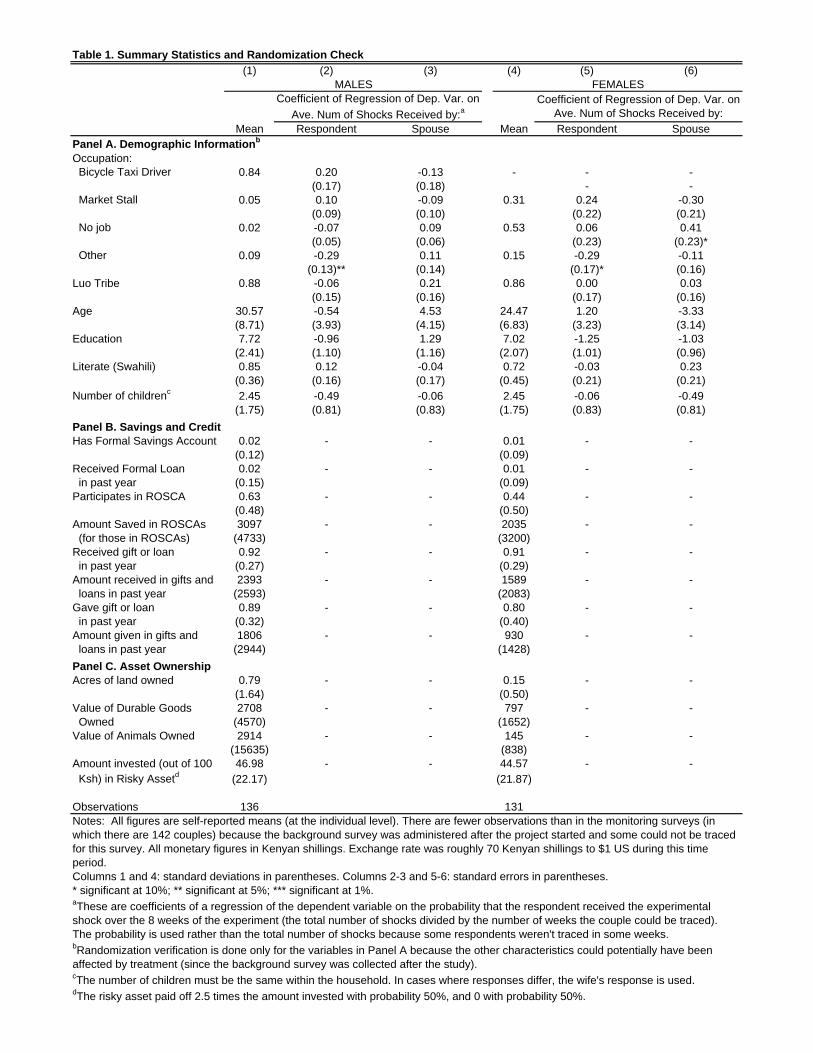
Table 1. Summary Statistics and Randomization Check

(1) (2) (3) (4) (5) (6)

Mean Respondent Spouse Mean Respondent SpousePanel A. Demographic Informationb

Occupation: Bicycle Taxi Driver 0.84 0.20 -0.13 - - -

(0.17) (0.18) - - Market Stall 0.05 0.10 -0.09 0.31 0.24 -0.30

(0.09) (0.10) (0.22) (0.21) No job 0.02 -0.07 0.09 0.53 0.06 0.41

(0.05) (0.06) (0.23) (0.23)* Other 0.09 -0.29 0.11 0.15 -0.29 -0.11

(0.13)** (0.14) (0.17)* (0.16)Luo Tribe 0.88 -0.06 0.21 0.86 0.00 0.03

(0.15) (0.16) (0.17) (0.16)Age 30.57 -0.54 4.53 24.47 1.20 -3.33

(8.71) (3.93) (4.15) (6.83) (3.23) (3.14)Education 7.72 -0.96 1.29 7.02 -1.25 -1.03

(2.41) (1.10) (1.16) (2.07) (1.01) (0.96)Literate (Swahili) 0.85 0.12 -0.04 0.72 -0.03 0.23

(0.36) (0.16) (0.17) (0.45) (0.21) (0.21)Number of childrenc 2.45 -0.49 -0.06 2.45 -0.06 -0.49

(1.75) (0.81) (0.83) (1.75) (0.83) (0.81)

Panel B. Savings and CreditHas Formal Savings Account 0.02 - - 0.01 - -

(0.12) (0.09)Received Formal Loan 0.02 - - 0.01 - - in past year (0.15) (0.09)Participates in ROSCA 0.63 - - 0.44 - -

(0.48) (0.50)Amount Saved in ROSCAs 3097 - - 2035 - - (for those in ROSCAs) (4733) (3200)Received gift or loan 0.92 - - 0.91 - - in past year (0.27) (0.29)Amount received in gifts and 2393 - - 1589 - - loans in past year (2593) (2083)Gave gift or loan 0.89 - - 0.80 - - in past year (0.32) (0.40)Amount given in gifts and 1806 - - 930 - - loans in past year (2944) (1428)

Panel C. Asset OwnershipAcres of land owned 0.79 - - 0.15 - -

(1.64) (0.50)Value of Durable Goods 2708 - - 797 - - Owned (4570) (1652)Value of Animals Owned 2914 - - 145 - -

(15635) (838)Amount invested (out of 100 46.98 - - 44.57 - - Ksh) in Risky Assetd (22.17) (21.87)

Observations 136 131

Coefficient of Regression of Dep. Var. on

Ave. Num of Shocks Received by:a

MALES FEMALESCoefficient of Regression of Dep. Var. on

Ave. Num of Shocks Received by:

Notes: All figures are self-reported means (at the individual level). There are fewer observations than in the monitoring surveys (in which there are 142 couples) because the background survey was administered after the project started and some could not be traced for this survey. All monetary figures in Kenyan shillings. Exchange rate was roughly 70 Kenyan shillings to $1 US during this time period.Columns 1 and 4: standard deviations in parentheses. Columns 2-3 and 5-6: standard errors in parentheses. * significant at 10%; ** significant at 5%; *** significant at 1%. aThese are coefficients of a regression of the dependent variable on the probability that the respondent received the experimental shock over the 8 weeks of the experiment (the total number of shocks divided by the number of weeks the couple could be traced). The probability is used rather than the total number of shocks because some respondents weren't traced in some weeks.bRandomization verification is done only for the variables in Panel A because the other characteristics could potentially have been affected by treatment (since the background survey was collected after the study).cThe number of children must be the same within the household. In cases where responses differ, the wife's response is used.dThe risky asset paid off 2.5 times the amount invested with probability 50%, and 0 with probability 50%.

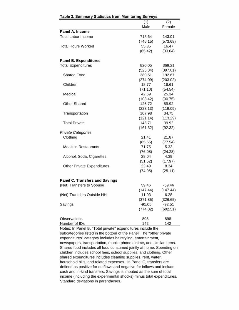
Table 2. Summary Statistics from Monitoring Surveys

(1) (2)Male Female

Panel A. IncomeTotal Labor Income 718.64 143.01

(746.15) (573.68)Total Hours Worked 55.35 16.47

(65.42) (33.04)

Panel B. ExpendituresTotal Expenditures 820.05 369.21

(525.34) (397.01) Shared Food 380.51 192.67

(274.09) (203.02) Children 18.77 16.61

(71.10) (54.54) Medical 42.59 25.34

(103.42) (90.75) Other Shared 126.72 59.92

(228.13) (119.09) Transportation 107.98 34.75

(121.14) (113.29) Total Private 143.71 39.92

(161.32) (92.32)Private Categories Clothing 21.41 21.87

(85.65) (77.54) Meals in Restaurants 71.75 5.33

(76.08) (24.28) Alcohol, Soda, Cigarettes 28.04 4.39

(51.52) (17.97) Other Private Expenditures 22.49 8.34

(74.95) (25.11)

Panel C. Transfers and Savings(Net) Transfers to Spouse 59.46 -59.46

(147.44) (147.44)(Net) Transfers Outside HH 11.03 6.28

(371.85) (326.65)Savings -91.05 -92.51

(774.02) (602.51)

Observations 898 898Number of IDs 142 142Notes: In Panel B, "Total private" expenditures include the subcategories listed in the bottom of the Panel. The "other private expenditures" category includes hairstyling, entertainment, newspapers, transportation, mobile phone airtime, and similar items. Shared food includes all food consumed jointly at home. Spending on children includes school fees, school supplies, and clothing. Other shared expenditures includes cleaning supplies, rent, water, household bills, and related expenses. In Panel C, transfers are defined as positive for outflows and negative for inflows and include cash and in-kind transfers. Savings is imputed as the sum of total income (including the experimental shocks) minus total expenditures. Standard deviations in parentheses.

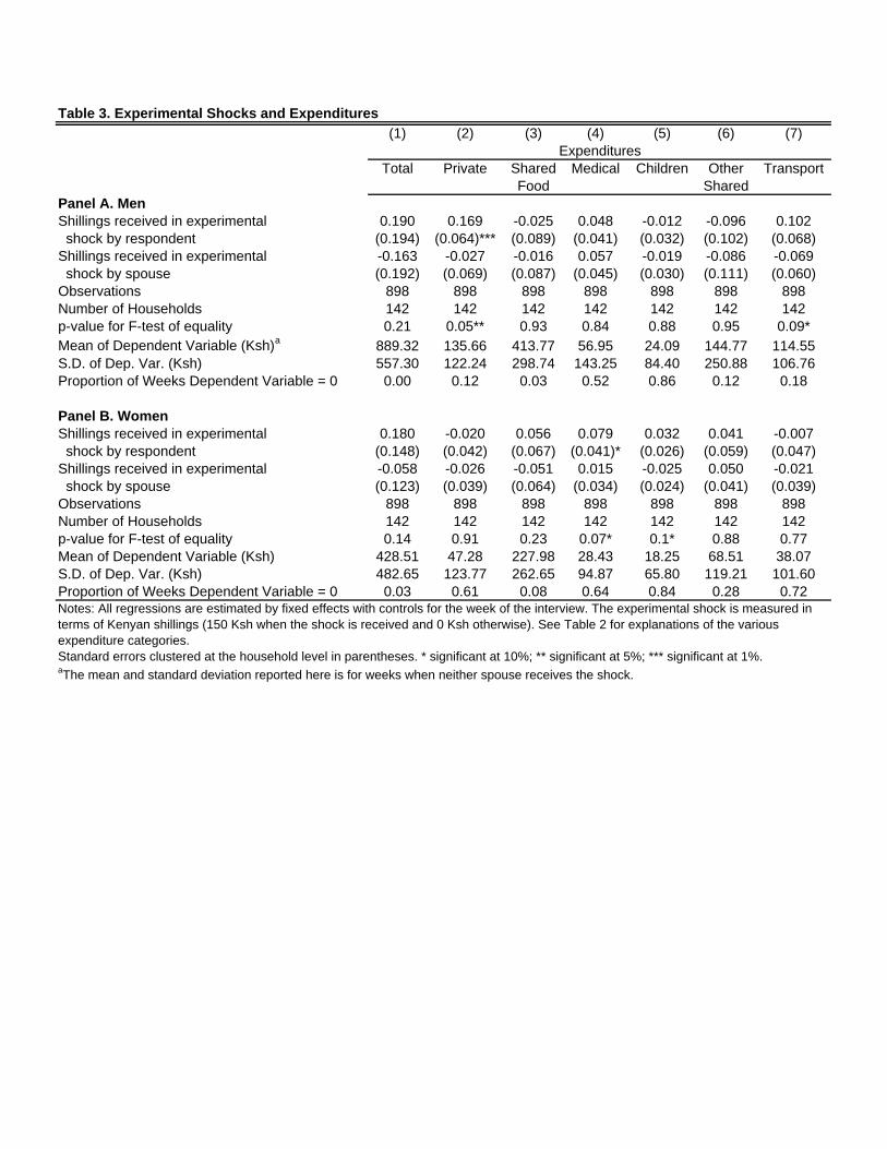
Table 3. Experimental Shocks and Expenditures

(1) (2) (3) (4) (5) (6) (7)

Total Private Shared Medical Children Other TransportFood Shared

Panel A. MenShillings received in experimental 0.190 0.169 -0.025 0.048 -0.012 -0.096 0.102 shock by respondent (0.194) (0.064)*** (0.089) (0.041) (0.032) (0.102) (0.068)Shillings received in experimental -0.163 -0.027 -0.016 0.057 -0.019 -0.086 -0.069 shock by spouse (0.192) (0.069) (0.087) (0.045) (0.030) (0.111) (0.060)Observations 898 898 898 898 898 898 898Number of Households 142 142 142 142 142 142 142p-value for F-test of equality 0.21 0.05** 0.93 0.84 0.88 0.95 0.09*Mean of Dependent Variable (Ksh)a 889.32 135.66 413.77 56.95 24.09 144.77 114.55S.D. of Dep. Var. (Ksh) 557.30 122.24 298.74 143.25 84.40 250.88 106.76Proportion of Weeks Dependent Variable = 0 0.00 0.12 0.03 0.52 0.86 0.12 0.18

Panel B. WomenShillings received in experimental 0.180 -0.020 0.056 0.079 0.032 0.041 -0.007 shock by respondent (0.148) (0.042) (0.067) (0.041)* (0.026) (0.059) (0.047)Shillings received in experimental -0.058 -0.026 -0.051 0.015 -0.025 0.050 -0.021 shock by spouse (0.123) (0.039) (0.064) (0.034) (0.024) (0.041) (0.039)Observations 898 898 898 898 898 898 898Number of Households 142 142 142 142 142 142 142p-value for F-test of equality 0.14 0.91 0.23 0.07* 0.1* 0.88 0.77Mean of Dependent Variable (Ksh) 428.51 47.28 227.98 28.43 18.25 68.51 38.07S.D. of Dep. Var. (Ksh) 482.65 123.77 262.65 94.87 65.80 119.21 101.60Proportion of Weeks Dependent Variable = 0 0.03 0.61 0.08 0.64 0.84 0.28 0.72Notes: All regressions are estimated by fixed effects with controls for the week of the interview. The experimental shock is measured in terms of Kenyan shillings (150 Ksh when the shock is received and 0 Ksh otherwise). See Table 2 for explanations of the various expenditure categories.Standard errors clustered at the household level in parentheses. * significant at 10%; ** significant at 5%; *** significant at 1%. aThe mean and standard deviation reported here is for weeks when neither spouse receives the shock.

Expenditures

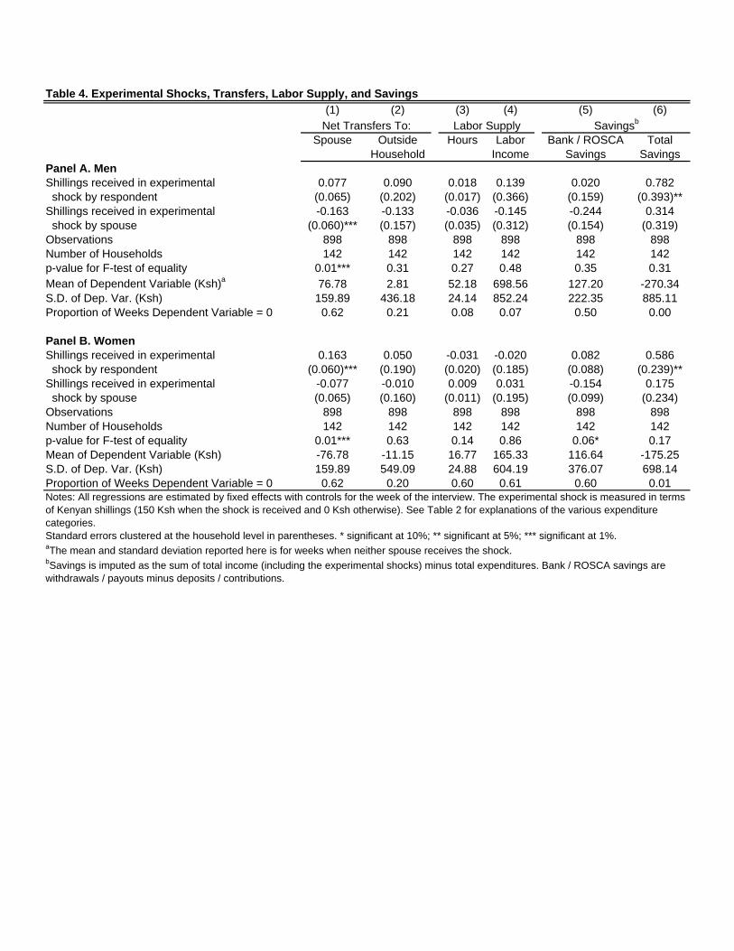
Table 4. Experimental Shocks, Transfers, Labor Supply, and Savings

(1) (2) (3) (4) (5) (6)

Spouse Outside Hours Labor Bank / ROSCA TotalHousehold Income Savings Savings

Panel A. MenShillings received in experimental 0.077 0.090 0.018 0.139 0.020 0.782 shock by respondent (0.065) (0.202) (0.017) (0.366) (0.159) (0.393)**Shillings received in experimental -0.163 -0.133 -0.036 -0.145 -0.244 0.314 shock by spouse (0.060)*** (0.157) (0.035) (0.312) (0.154) (0.319)Observations 898 898 898 898 898 898Number of Households 142 142 142 142 142 142p-value for F-test of equality 0.01*** 0.31 0.27 0.48 0.35 0.31Mean of Dependent Variable (Ksh)a 76.78 2.81 52.18 698.56 127.20 -270.34S.D. of Dep. Var. (Ksh) 159.89 436.18 24.14 852.24 222.35 885.11Proportion of Weeks Dependent Variable = 0 0.62 0.21 0.08 0.07 0.50 0.00

Panel B. WomenShillings received in experimental 0.163 0.050 -0.031 -0.020 0.082 0.586 shock by respondent (0.060)*** (0.190) (0.020) (0.185) (0.088) (0.239)**Shillings received in experimental -0.077 -0.010 0.009 0.031 -0.154 0.175 shock by spouse (0.065) (0.160) (0.011) (0.195) (0.099) (0.234)Observations 898 898 898 898 898 898Number of Households 142 142 142 142 142 142p-value for F-test of equality 0.01*** 0.63 0.14 0.86 0.06* 0.17Mean of Dependent Variable (Ksh) -76.78 -11.15 16.77 165.33 116.64 -175.25S.D. of Dep. Var. (Ksh) 159.89 549.09 24.88 604.19 376.07 698.14Proportion of Weeks Dependent Variable = 0 0.62 0.20 0.60 0.61 0.60 0.01

Net Transfers To: Labor Supply Savingsb

Notes: All regressions are estimated by fixed effects with controls for the week of the interview. The experimental shock is measured in terms of Kenyan shillings (150 Ksh when the shock is received and 0 Ksh otherwise). See Table 2 for explanations of the various expenditure categories.Standard errors clustered at the household level in parentheses. * significant at 10%; ** significant at 5%; *** significant at 1%. aThe mean and standard deviation reported here is for weeks when neither spouse receives the shock.bSavings is imputed as the sum of total income (including the experimental shocks) minus total expenditures. Bank / ROSCA savings are withdrawals / payouts minus deposits / contributions.

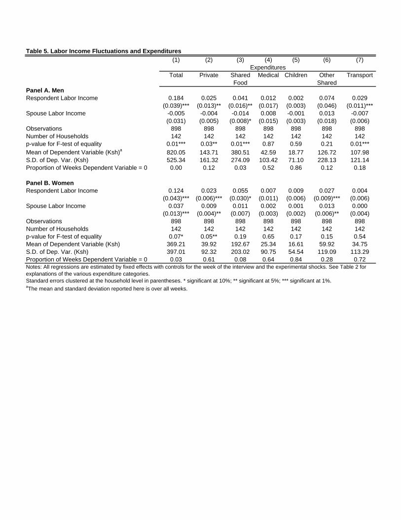
Table 5. Labor Income Fluctuations and Expenditures

(1) (2) (3) (4) (5) (6) (7)

Total Private Shared Medical Children Other TransportFood Shared

Panel A. MenRespondent Labor Income 0.184 0.025 0.041 0.012 0.002 0.074 0.029

(0.039)*** (0.013)** (0.016)** (0.017) (0.003) (0.046) (0.011)***Spouse Labor Income -0.005 -0.004 -0.014 0.008 -0.001 0.013 -0.007

(0.031) (0.005) (0.008)* (0.015) (0.003) (0.018) (0.006)Observations 898 898 898 898 898 898 898Number of Households 142 142 142 142 142 142 142p-value for F-test of equality 0.01*** 0.03** 0.01*** 0.87 0.59 0.21 0.01***Mean of Dependent Variable (Ksh)a 820.05 143.71 380.51 42.59 18.77 126.72 107.98S.D. of Dep. Var. (Ksh) 525.34 161.32 274.09 103.42 71.10 228.13 121.14Proportion of Weeks Dependent Variable = 0 0.00 0.12 0.03 0.52 0.86 0.12 0.18

Panel B. WomenRespondent Labor Income 0.124 0.023 0.055 0.007 0.009 0.027 0.004

(0.043)*** (0.006)*** (0.030)* (0.011) (0.006) (0.009)*** (0.006)Spouse Labor Income 0.037 0.009 0.011 0.002 0.001 0.013 0.000

(0.013)*** (0.004)** (0.007) (0.003) (0.002) (0.006)** (0.004)Observations 898 898 898 898 898 898 898Number of Households 142 142 142 142 142 142 142p-value for F-test of equality 0.07* 0.05** 0.19 0.65 0.17 0.15 0.54Mean of Dependent Variable (Ksh) 369.21 39.92 192.67 25.34 16.61 59.92 34.75S.D. of Dep. Var. (Ksh) 397.01 92.32 203.02 90.75 54.54 119.09 113.29Proportion of Weeks Dependent Variable = 0 0.03 0.61 0.08 0.64 0.84 0.28 0.72

Expenditures

Notes: All regressions are estimated by fixed effects with controls for the week of the interview and the experimental shocks. See Table 2 for explanations of the various expenditure categories.Standard errors clustered at the household level in parentheses. * significant at 10%; ** significant at 5%; *** significant at 1%. aThe mean and standard deviation reported here is over all weeks.

Table 6. Labor Income Fluctuations, Transfers, and Savings

(1) (2) (3) (4)

Spouse Outside Bank / ROSCA TotalHousehold Savings Savings

Panel A. MenRespondent Labor Income -0.006 0.089 -0.043 0.733

(0.010) (0.041)** (0.065) (0.075)***Spouse Labor Income 0.008 -0.011 -0.001 0.008

(0.014) (0.020) (0.023) (0.039)Observations 898 898 898 898Number of Households 142 142 142 142p-value for F-test of equality 0.54 0.02** 0.57 0.01***Mean of Dependent Variable (Ksh)a 59.46 11.03 109.90 -91.05S.D. of Dep. Var. (Ksh) 147.44 371.85 355.49 774.02Proportion of Weeks Dependent Variable = 0 0.62 0.21 0.50 0.00

Panel B. WomenRespondent Labor Income -0.008 0.081 -0.011 0.803

(0.014) (0.023)*** (0.016) (0.049)***Spouse Labor Income 0.006 -0.024 0.013 -0.018

(0.010) (0.014)* (0.044) (0.019)Observations 898 898 898 898Number of Households 142 142 142 142p-value for F-test of equality 0.54 0.01*** 0.60 0.001***Mean of Dependent Variable (Ksh) -59.46 6.28 92.36 -92.51S.D. of Dep. Var. (Ksh) 147.44 326.65 307.46 602.51Proportion of Weeks Dependent Variable = 0 0.62 0.20 0.60 0.01

Net Transfers To: Savingsb

Notes: All regressions are estimated by fixed effects with controls for the week of the interview and the experimental shocks. See Table 2 for explanations of the various expenditure categories.Standard errors clustered at the household level in parentheses. * significant at 10%; ** significant at 5%; *** significant at 1%. aThe mean and standard deviation reported here is over all weeks.bSavings is imputed as the sum of total income (including the experimental shocks) minus total expenditures. Bank / ROSCA savings are withdrawals / payouts minus deposits / contributions.