Lightning Induced Voltages on Overhead Lines …Lightning Induced Voltages on Overhead Lines above...
138
Lightning Induced Voltages on Overhead Lines above Non-Uniform and Non- Homogeneous Ground Author Raúl Esteban Jiménez Mejía Master Thesis Dissertation Universidad Nacional de Colombia Departamento de Energía Eléctrica y Automática Facultad de Minas November 2014
Transcript of Lightning Induced Voltages on Overhead Lines …Lightning Induced Voltages on Overhead Lines above...
Lightning Induced Voltages on Overhead
Lines above Non-Uniform and Non-
Homogeneous Ground
Author
Raúl Esteban Jiménez Mejía
Master Thesis Dissertation
Universidad Nacional de Colombia
Departamento de Energía Eléctrica y Automática
Facultad de Minas
November 2014
Lightning Induced Voltages on Overhead
Lines above Non-Uniform and Non-
Homogeneous Ground
Author
Raúl Esteban Jiménez Mejía
Master Thesis Dissertation
Presented as a partial fulfillment of the requirements for the degree of
Master on Electrical Engineering
Advisor
Prof. Javier Gustavo Herrera Murcia, Ph.D.
Universidad Nacional de Colombia
Departamento de Energía Eléctrica y Automática
Facultad de Minas
November 2014

Gratefulness: To my Parents

i
Acknowledgments
There are many people that I must be grateful with by all of their attention and comprehension
along these two years. I would like to express my sincere gratitude to all of those that have been
there offering me their valuable comments and assistance during the development of this thesis.
Along the time working on it, I have learned not only about lighting induced voltages but also that
when you are with a good working group and excellent people around you, there are more
probabilities to succeed.
I wish to thank Prof. Javier Herrera for accepting to be the advisor of this work and the way how
he from the first time offered me all his experience on lightning research for the development of
this thesis.
I really have to highlight all the support that I have received from the Research Group on Applied
Technologies (GITA) and express my especial gratitude to Prof. Guillermo Mesa who has been a
very important advisor not only academically but also as a real and sincere friend. I would also like
to thank to Prof. Clara Rojo for all of her valuable advices and her support whereas I held my
position as teaching assistant of the high voltage laboratory.
My sincere gratitude to my parents for all of their confidence on me and on my work. Special
thanks to my brother David who has given me important advices along this work and to Stephanie
who has been present to encourage me along this two years.
I am sincerely grateful to my teamwork and friends: Gilbert, Camilo and Juan Fernando for backing
me up when I was unavailable and for all of their valuable suggestions and encouragements.
Finally, I would also like to address my gratitude to all of my old friends and colleagues for their
valuable assistance and comments.

ii
Abstract
Lightning induced voltages are one of the most common sources of failures on distribution
networks operating in high lightning activity regions. Traditionally, the selection of insulation levels
and protecting devices are carried out using statistical analysis based on typical values of resistivity
and assuming a homogeneous ground for the whole network. In calculating lightning induced
voltages, the effect of the topography and non-homogeneities of the ground have been
traditionally neglected.
In rural distribution lines, non-homogeneous and non-uniform ground is a common feature. In
literature, induced voltages calculations are mainly calculated based on several assumptions that
are not valid when more realistic conditions are taken into account. In order to allow a better
selection of protective devices and hence contributing to the improvement of some power quality
indicators of rural distribution networks, the calculation of lightning induced voltages for
distribution lines must be performed including the effects of the non-homogeneous and non-
uniform ground.
Most of the theoretical approaches proposed for calculating the propagation path effects on the
radiated electromagnetic fields for a current dipole above ground, are valid only in the far-field
region even when considering irregular and inhomogeneous terrain. Despite some authors have
demonstrated the validity of those approaches for flat ground in the near field range calculations,
there are valid for some specific cases and geometric symmetry that in some practical cases
cannot be assumed.
In order to overcome this problem, this thesis presents an extensive application of a full wave
solution obtained from the implementation of the Finite Difference Time Domain (FDTD) method
including a non-regular mesh. This method is applied to the calculation of lightning induced
voltages on an overhead single wire when different ground features such as: homogeneity,
inhomogeneity and non-uniformity are present all simultaneously in a simulation scenario. In
order to validate the FDTD implementation, some numerical comparisons were made with
previous results presented in the literature.
The aim of this thesis is to provide new elements related to the effects on lighting induced
voltages on overhead lines when different electric and geometric parameters of the surrounding
ground are considered. Along this thesis, the lightning induced voltage problem has been analyzed
taking into account three involved aspects individually: the return-stroke model, the propagation
of the electromagnetic field produced by it, and the resulting induced voltages on the overhead
lines once all their models are included into an FDTD simulation.
This document has been divided into eight sections. The first section presents a discussion about
lightning induced voltages and how they have been addressed in the literature. Throughout this
iii
section all the involved elements into the lighting induced problem have been addressed and a
short discussion about their previous results and conclusions is also presented.
In section 2 the scope of the thesis is defined in order to give the reader a brief summary about
the objectives that were established in the master thesis proposal.
Section 3 presents the FDTD method. In this section most of the theoretical background is
presented related to: sources, lumped elements and thin-wire modeling techniques. Next, the
FDTD method is formulated for a non-regular mesh and a general formulation for an automatic
meshing algorithm is proposed. Finally, a comparison between the FDTD method implementation
used in this thesis and some experimental data from a two horizontal wires cross-talk problem is
presented.
Section 4 deals with the calculation of radiated fields when different propagation paths are
present. Homogeneous ground effects on radiated fields were obtained by using the Norton’s
approach and the surface impedance concept. Inhomogeneities of the ground conductivity for flat
grounds were also analyzed by using the surface impedance concept and the Wait´s formula
derived from the compensation theorem; the Wait´s formulas for a mixed-path of two and three
section were implemented and compared with some results presented before in literature. Finally,
the terrain non-uniformity was addressed by means of the Ott’s integral approach. Despite all of
these implemented approaches allow the analysis of radiated fields, they are derived under
several assumptions and are valid only for the far field region and a cylindrical symmetry regarding
geometry. Then, a comparison between these and the results obtained by means of the FDTD
method were performed for different simulation scenarios in order to analyze their validity.
In section 5 the lightning return-stroke is modeled by means of an implementation of engineering
and electromagnetic models. A discussion about the current distribution along the channel
depending on the return-stroke model is also presented. Besides, a comparison between the
antenna theory and the series RL-loaded thin-wire model included into the FDTD method was
carried out taking into account the characteristics of apparent propagation velocity and current
wave shape along the channel.
In section 6 the lightning radiated fields are calculated for different propagation path conditions
such as: perfectly conducting ground, homogeneous finitely conductive ground and
inhomogeneous conducting ground. For those propagation paths a set of comparisons between
the FDTD method and the approximated formulas discussed in section 5 were performed.
Lightning induced voltages are analyzed in section 7. In this section the lightning channel and the
overhead line are included into the FDTD method. A set of simulations scenarios were proposed in
order to evaluate the influence of different ground features on the induced voltages on a single
overhead-wire. Important influences on induced voltage waveforms were determined for
inhomogeneous and irregular terrains, resulting in changes on polarity and higher induced peak
voltages values when compared to those obtained from a flat homogeneous ground.

iv
In section 8 concluding remarks about the analyzed cases and most critical situations are
presented. There is also a future work proposed by the author based on the obtained results.

v
Table of Contents
Lightning Induced Voltages on Overhead Lines above Non-Uniform and Non-Homogeneous
Ground ..................................................................................................................................................
Lightning Induced Voltages on Overhead Lines above Non-Uniform and Non-Homogeneous
Ground ................................................................................................................................................. i
Gratefulness: To my Parents ............................................................................................................ ii
Acknowledgments ................................................................................................................................ i
Abstract ............................................................................................................................................... ii
Table of Figures ................................................................................................................................. viii
1 The Lighting Induced Voltage Problem: State of the Art Discussion .......................................... 1
2 Scope of the Thesis ...................................................................................................................... 5
3 The Finite Difference Time-Domain Method for Electromagnetic Fields ................................... 6
3.1 Maxwell´s Equations and Electromagnetic Fields ............................................................... 6
3.2 Numerical Solution of the Maxwell´s Equations ................................................................. 7
3.3 Numerical Stability Criteria ................................................................................................. 9
3.4 Media Modeling ................................................................................................................ 10
3.5 Lumped Elements Modeling ............................................................................................. 12
3.5.1 Sources Modeling ...................................................................................................... 13
3.5.2 Resistor ...................................................................................................................... 15
3.5.3 Inductor ..................................................................................................................... 16
3.5.4 Capacitor ................................................................................................................... 17
3.5.5 Series RL load ............................................................................................................ 17
3.5.6 Parallel RC load .......................................................................................................... 19
3.6 Boundary Conditions ......................................................................................................... 20
3.6.1 Perfectly Conductive Boundary Condition ................................................................ 21
3.6.2 Absorbing Boundaries Conditions ............................................................................. 22
3.6.3 PML and CPML Boundaries ....................................................................................... 30
3.7 Thin-Wire Modeling .......................................................................................................... 32
3.7.1 Umashanark´s Model (UM) ....................................................................................... 32

vi
3.7.2 Noda-Yokoyamas’s Model (NY) ................................................................................. 35
3.7.3 Limit of Stability of the NY-Thin Wire ........................................................................ 38
3.7.4 Improved Noda-Yokoyama Model (INY) ................................................................... 39
3.8 Non-Regular mesh into the FDTD method ........................................................................ 41
3.8.1 The FDTD Method in a Non-regular Mesh ................................................................ 41
3.8.2 Automatic-Mesh Algorithm ....................................................................................... 43
3.9 Experimental Validation Case: – The Cross-Talk Effect. .................................................... 47
3.9.1 Simulation by FDTD using a Regular Mesh ................................................................ 51
3.9.2 Simulation by FDTD using a Non-Regular Mesh ........................................................ 52
4 Radiated Electromagnetic Field ................................................................................................ 55
4.1 Radiating Vertical-Current Dipole over a homogeneous ground. ..................................... 55
4.1.1 Radiation above a perfectly conductive Ground ....................................................... 57
4.1.2 Radiation above a Flat Homogeneous ground .......................................................... 58
4.2 Radiating Vertical-Current Dipole over an Inhomogeneous and Irregular Ground (far-field
region). .......................................................................................................................................... 62
4.2.1 Green´s Theorem Approach ...................................................................................... 62
4.2.2 Radiation fields over an inhomogeneous ground. .................................................... 64
4.2.3 Radiation fields over an irregular ground. ................................................................ 68
4.3 Radiating Vertical-Current Dipole over an Inhomogeneous and Irregular Ground (near-
field region). .................................................................................................................................. 70
4.3.1 Radiated Fields over Homogeneous and Inhomogeneous Flat Ground ................... 71
4.3.2 Radiated Fields over Irregular Ground ...................................................................... 74
5 Lightning Return-Stroke Modeling ............................................................................................ 77
5.1 Engineering Models ........................................................................................................... 77
5.2 Electromagnetic Models ................................................................................................... 78
5.3 Lightning Channel as a Loaded Thin-wire.......................................................................... 80
6 Propagation Path Effects on Lightning Radiated Fields ............................................................ 83
6.1 Perfectly Conducting Ground ............................................................................................ 83
6.2 Homogeneous Lossy Ground ............................................................................................ 86
6.3 Non-homogeneous Ground .............................................................................................. 92
6.3.1 Mixed-Path ground ................................................................................................... 92
7 Lightning Induced Over-voltages............................................................................................... 98

vii
7.1 Overhead Line Modeling and Electromagnetic Coupling .................................................. 99
7.1.1 Perfectly Conducting Ground and Homogeneous Ground ....................................... 99
7.1.2 In-homogeneous Ground ........................................................................................ 100
7.1.3 Non-Uniform Ground Effect .................................................................................... 108
8 Conclusions Remarks and Future work ................................................................................... 119
9 References ............................................................................................................................... 121

viii
Table of Figures
Figure 1 Yee's cell for the electric and magnetic fields location in space. .......................................... 7
Figure 2 Leapfrog scheme in time for updating electric and magnetic fields. .................................... 8
Figure 3 Material Inclusion into the Yee’s Cell .................................................................................. 11
Figure 4 Source Modeling into the Yee´s Cell (a) Lumped Voltage Source with non-zero internal
impedance (b) Current Source .......................................................................................................... 13
Figure 5 Resistor Modeling into the Yee´s Cell ................................................................................. 15
Figure 6 Inductor Modeling into the Yee´s Cell ................................................................................. 16
Figure 7 Capacitor Modeling into the Yee´s Cell ............................................................................... 17
Figure 8 Lumped RL-Load Modeling into the Yee´s Cell .................................................................... 18
Figure 9 Parallel RC-lumped Load into the Yee´s Cell ....................................................................... 19
Figure 10 Electric Field Components calculation at the Boundary of the Computational Domain .. 20
Figure 11 (a) Simulation Set-up for PEC Boundaries Implementation (b) Source Waveform (c)
Electric Field Magnitudes for each component at the Receiver Point (d) Magnetic Field magnitudes
for each component at the Receiver Point ....................................................................................... 22
Figure 12 Geometric Interpretation of an incident wave for the Mur’s Boundary Conditions
derivation .......................................................................................................................................... 23
Figure 13 Vertical Electric Field contour plot of an oscillating vertical current dipole by using Mur’s
Boundaries as ABCs (a) Contour Radiation Pattern for the first Order and second order
approximation presented in [33] (b) 1st Order and 2nd Order Mur’s Boundaries implementation . 27
Figure 14 One-Dimensional propagating wave calculated at discrete time-spatial locations .......... 28
Figure 15 Liao´s Boundaries performance compared with (a) Mur´s Boundaries (2nd Order)
Boundaries (b) Liao’s Boundaries (2nd Order) (c) Contour plot comparison ..................................... 29
Figure 16 Comparison between ABCs boundaries implementations (a) Gaussian’s Pulse Excitation
(b) Mur’s and CPML ABCs (Solid: Mur’s 2nd Order 3D Boundaries, Circles: CPML) (c) Performance
Comparison between Liao’s and CPML ABCs (Solid: Liao’s 2nd Order Boundaries, Circles: CPML) ... 31
Figure 17 Thin-wire segment inclusion into the Yee´s cell ................................................................ 32
Figure 18 Segment of a z-directed wire ............................................................................................ 33
Figure 19 Thin-wire inclusion in the Yee´s cube ................................................................................ 35
Figure 20 Permittivity and Permeability components modifications for the NY thin-wire model ... 36
Figure 21 Experimental Set-up geometry for a Horizontal conductor above a Cooper Plate (from
[41]) ................................................................................................................................................... 36
Figure 22 Thin-wire Representation (a) Voltage Source Waveform (b) Voltages at the near and far
end of the line (c) Current Waveform at the source ......................................................................... 37
Figure 23 Comparison between the TEM approach and the FDTD calculations (dashed: TEM
Approach, Solid: FDTD) (a) Voltages along the Line (b) Current at the source ................................. 38
Figure 24 Instability condition for radius lower than 0.15 times the cell-side size .......................... 39
Figure 25 Voltages along the Line by using the Improved Thin-Wire Formulation .......................... 40
Figure 26 Voltages at the near and far end of the Line (a) Thin Wire placed on the X-axis direction
........................................................................................................................................................... 40

ix
Figure 27 Location of the electric and magnetic field component in the non-regular cell ............... 42
Figure 28 Spacing Function and Coordinate Points function ............................................................ 44
Figure 29 Parabolic Mesh based on a trapezoidal spacing function ................................................. 45
Figure 30 Parabolic Mesh Algorithm (a) Example of a Spacing Function (b) Coordinate mesh nodes
........................................................................................................................................................... 46
Figure 31(a) Schematic Representation of capacitive coupling for two wires above a conductive
return plate (cross section). (b) Schematic Representation of inductive coupling for two wires
above a conductive return plate (lateral section) ............................................................................. 48
Figure 32 Typical Cross-talk Simulation scenario for two horizontal parallels wires (a) Schematic
Representation of the experimental set-up (b) Experimental set-up. .............................................. 49
Figure 33 Measured Voltages on the Generator and the Victim Wire for the performed Cross-talk
Experiment (a) Voltage on the load of the generator Wire (b) Victim Wire Voltages at the near and
far end ............................................................................................................................................... 50
Figure 34 (a) Circuital model for the scope probe used in the measurements (b) Frequency
response of the circuital model for the scope probe ........................................................................ 51
Figure 35 Voltages for a typical Cross-Talk set-up of two parallel conductor with 1.5cm of
Separation (Dashed Line: ATP/EMTP, Solid Line: FDTD) (a) Voltages on Generator Wire (b) Voltages
on Victim Wire at the near and far end. ........................................................................................... 52
Figure 36 Victim Wire Induced Voltage (Dashed Line: ATP/EMTP, Solid Line: FDTD, Dotted:
Measured) (a) Comparison between measured and TEM approach at source and load voltage
(1.5cm of separation) (b) Comparison between measured and TEM approach at near and far end
voltage (1.5cm of separation). .......................................................................................................... 52
Figure 37 Irregular Meshing for the FDTD simulation (a) Top View (XY) (b) Lateral View (XZ) ........ 53
Figure 38 Voltages on the Victim Wire (dotted: Measured, solid: FDTD non-regular mesh) (a)
Voltage at the Near End (b) Voltage at the Far End .......................................................................... 54
Figure 39 (a) Dipole Antenna (b) Current Distribution for a half-wave dipole (c) Current-Element
Dipole ................................................................................................................................................ 55
Figure 40 Vertical electric current dipole radiation in the free-Space .............................................. 56
Figure 41 Radiation above perfectly conducting ground .................................................................. 57
Figure 42 Vertical Current Dipole above Homogeneous Finitely Conducting Ground ..................... 58
Figure 43 Attenuation Function Magnitude Comparison for a Vertical Current-Dipole above a Flat
Homogeneous Ground. Norton Approach (dashed lines) and Sommerfeld’s solution (circles) taken
from [52] ........................................................................................................................................... 61
Figure 44 Radiated Horizontal Electric Field (10m in height) along the propagation path .............. 62
Figure 45 Relevant Geometry Irregular Terrain profile. ................................................................... 63
Figure 46 (a) Two-Sections Mixed-Path Condition (b) Three-Section Mixed-Path ........................... 65
Figure 47 Attenuation Function for a Mixed-Path (dashed: Wait´s Approach, circles: Ott’s integral
presented in [54]) (a) Relevant Geometry for three section Mixed-Path (b) Wait’s Attenuation
Function for Two Sections ρ1=0.5Ωm/ ρ2=500Ωm (c) Wait’s Attenuation Function for Three-
Sections ρ1=0.5Ωm/ ρ2=500Ωm / ρ3=0.5Ωm ................................................................................... 67
Figure 48 Radiated Electric Field Components along the Path at 10m in height (a) Horizontal
Electric Field Component (b) Vertical Electric Field Component ...................................................... 67

x
Figure 49 Irregular Propagation Path and their Attenuation Function Magnitude. (a) Ridge Terrain
Profile (b) Attenuation Function for a Ridge Terrain Profile (c) Cliff Terrain Profile (d) Attenuation
Function for a Cliff Terrain Profile ..................................................................................................... 69
Figure 50 Irregular Ground Effect on Radiated Electric Fields. Gaussian Ridge: (a) Horizontal Electric
Field (b) Vertical Electric Field. Gaussian Cliff: (c) Horizontal Electric Field (d) Vertical Electric Field
........................................................................................................................................................... 70
Figure 51 Horizontal Electric Field Component due to a vertical current dipole within the Near Field
Range (circles: FDTD, cross: Wait´s Approach) (a) Homogeneous Case (b) Two-Section Mixed path
(c) Three Section Mixed-path ............................................................................................................ 72
Figure 52 Attenuation Function influence in the near-field Horizontal Electric Field Calculation ... 73
Figure 53 Attenuation Function Magnitude Frequency Response at different distances from the
radiating dipole (gray lines: 1000Ωm, black lines: 100Ωm) .............................................................. 73
Figure 54 Validity of the Wait formula for Mixed-Path of Three sections (a) Horizontal Electric Field
........................................................................................................................................................... 74
Figure 55 Irregular ground effect on radiated field in the near field (a) Ground Profile along the x-
axis included into the FDTD method (b) Horizontal electric field from the current dipole location
along an abrupt profile change for different oscillating frequencies (dashed: Homogeneous, black
empty circle: 1MHz, gray filled circles: 5MHz , black filled circles: 10MHz) ..................................... 75
Figure 56 Current Propagation by means of the MTLE with λ=2000, v=c/2 ..................................... 78
Figure 57 Longitudinal Current Propagation for a Vertical Thin-Wire with radius 0.3m (solid line:
NEC-4, dashed: FDTD) ....................................................................................................................... 79
Figure 58 Current Distribution along a Thin-Wire inductance-loaded (Solid line: FDTD
implementation, circles line: Results presented in [6]). ................................................................... 80
Figure 59 Current Propagation along the Lightning Channel (solid line: NEC-4, dashed: FDTD) ...... 81
Figure 60 Comparison between the MLTE and RL loaded thin-wire for return stroke models (solid:
base channel current, solid grayed: RL-loaded thin-wire, dashed: MTLE λ=2km) ............................ 82
Figure 61 FDTD Non-regular mesh distribution (a) Top View (Plane XY) (b) Side View (Plane XZ) ... 84
Figure 62 Current Distribution along the Lightning Channel RL loaded Return-Stroke model (solid
grayed: NEC-4, dashed line: FDTD-Thin Wire RL loaded) .................................................................. 85
Figure 63 Lightning Radiated Fields above Perfectly Conducting Ground, Horizontal Electric Field
(Solid Line: Theoretical, Dashed Line: FDTD) (a) Hor. Electric Field Range I (closer distances than
200m to the Channel Base) (b) Hor. Electric Field Range II (longer distances than 500m to the
Channel Base) .................................................................................................................................... 85
Figure 64 Horizontal Electric field at 10m height above a lossy ground of resistivity 1000Ωm at a
distance of 200m from the stroke modeled by MLTE (dashed: Norton Approach, circles:
Sommerfeld’s taken from *20+) ......................................................................................................... 86
Figure 65 Radiated Electric Fields above different Ground Resistivity values (a) Vertical Electric
Field (b) Horizontal Electric Field for distances closer than 200m (c) Horizontal Electric Field for
distances further than 500m ............................................................................................................. 88
Figure 66 Horizontal Electric Field Component with different lightning return-stroke model (solid:
RL Thin-Wire, dashed: MLTE) (a) Current distribution along the Channel (b) Electric Field

xi
Component at distances closer than 200m (c) Electric Field Component at distances further than
500m ................................................................................................................................................. 89
Figure 67 Horizontal Electric field at 10m height above a lossy ground of resistivity 100Ωm at two-
different distances from the channel modeled by RL Loaded Thin-Wire (a) at distance of 100m (b)
at distance of 1km (dashed: Norton Approach, circles: FDTD taken from [70]) ............................... 90
Figure 68 Top View of the non-regular FDTD Meshing of the Problem Space ................................. 91
Figure 69 Horizontal Electric field at 10m height above a lossy ground of resistivity 100Ωm
(dashed: FDTD non-regular Mesh, Solid: Norton´s Approach) (a) Distances closer than 200m (b)
Distances further than 200m ............................................................................................................ 92
Figure 70 two-section mixed-path (solid: Homogeneous Case, dashed: Mixed-path condition) (a)
Relevant geometry of the Mixed-path of two section under analysis (b) Horizontal Electric field (c)
Vertical Electric field.......................................................................................................................... 93
Figure 71 Mixed-Path of three sections for lightning radiated fields (solid: Homogeneous Case,
dashed: Mixed-path condition) (a) Relevant geometry of the Mixed-path of three sections under
analysis (b) Horizontal Electric field (c) Vertical Electric field ........................................................... 94
Figure 72 Lightning Radiated Fields Mixed-Path of Two-Section calculated by the FDTD method.
Case 1 (Gray line): 10Ωm / 1000Ωm, Case 2 (Black line): 1000Ωm / 10Ωm (a) Simulation Set-Up (b)
Horizontal Electric Field (c) Vertical Electric Field ............................................................................. 95
Figure 73 Radiated Electric Field Components along a Mixed-Path of two-sections. (Dashed Line:
Wait’s Formulas, Solid Line: FDTD Method) Case 1: 10 Ωm / 1000 Ωm (a) Hor. Electric Field (b) Ver.
Electric Field, Case 2: 1000 Ωm / 10Ωm (c) Hor. Electric Field (d) Ver. Electric Field Case ............... 96
Figure 74 Calculated Induced Voltages on a 1km at 50m from the lightning strike (solid: FDTD,
circles: presented in [76]) ................................................................................................................ 100
Figure 75 Simulation setup for the induced voltage calculation on an overhead transmission line
above vertically stratified ground due to a lightning channel at 50m of one of the ends (near end
NE) and both ends connected to a resistor of 150Ω. ...................................................................... 101
Figure 76 Electric field components above the second mixed path section (Black: 10 Ωm / 1000 Ωm
case, Gray 1000 Ωm / 10 Ωm case) (a) Horizontal electric field over a mixed-path ground (b)
Vertical electric field over a mixed-path ground ............................................................................ 102
Figure 77 (a) Induced voltage at near end (b) Induced voltage at far end. ................................... 103
Figure 78 (a) Reflection factor magnitude (b) Reflection factor phase.......................................... 104
Figure 79 (a) Relevant geometry of the simulation set-up (b) Comparison of the induced voltages
by using the FEM method and the FDTD method (circles: FEM, solid: FDTD) ................................ 106
Figure 80 Induced Voltages for a Three-section mixed-path (a) Near End (b) Far End .................. 107
Figure 81 Geometry for the calculation of the induced voltages for a lightning strike on the top of a
step mountain (Solid: Flat Ground, Dashed: Irregular Ground) (a) Relevant Geometry for the
simulation set-up (b) Side view along the center of the mountain along the X-axis direction (c)
Induced voltage at the near-end (d) induced voltage at the far-end ............................................. 109
Figure 82 Geometry for the calculation of the induced voltages for a lightning strike on the bottom
of a step mountain (Solid: Flat Ground, Dashed: Irregular Ground) (a) Relevant Geometry for the
simulation set-up (b) Side view along the center of the mountain along the X-axis direction (c)
Induced voltage at the near-end (d) induced voltage at the far-end ............................................. 110

xii
Figure 83 Geometry for the calculation of the induced voltages for a lightning strike on the top of a
Gaussian Mountain (a) Relevant Geometry for the simulation set-up (b) Side view along the center
of the mountain along the X-axis direction (c) Side view along the center of the mountain along the
Y-axis direction ................................................................................................................................ 111
Figure 84 Induced voltages at near and far end due to a lightning strike on the top of a mountain
(Solid Line: Flat Ground case with FEM, Dashed: Gaussian Mountain with FDTD, Circles: cone-
shaped mountain with FEM presented in [28]) .............................................................................. 112
Figure 85 Overhead Line on the top of a mountain ........................................................................ 113
Figure 86 Induced Voltage for an Overhead Line on the top of a mountain (Solid Line: Flat Ground
Case, Dashed: non-uniform ground) ............................................................................................... 113
Figure 87 Induced Voltage for an Overhead Line with a mountain behind it (a) Relevant Geometry
(b) Induced Voltage for an Overhead Line with a mountain behind (Solid Line: Flat Ground Case,
Dashed: non-uniform ground) ........................................................................................................ 114
Figure 88 Overhead Line on between the top of two mountains (a) Relevant Geometry of the
scenario (b) Side View ..................................................................................................................... 115
Figure 89 Induced Voltage for an Overhead Line between the tops of two mountains (Solid Line:
Flat Ground Case, Dashed: non-uniform ground) ........................................................................... 115
Figure 90 Characteristic impedance of a single-wire overhead line above 1000Ωm lossy ground
depending on the conductor height by using the TEM approach .................................................. 116
Figure 91 (a) Description of the Simulation Set-up for the irregular ground effects on induced
voltages (b) Side View of the simulation set-up (c) Induced Voltage Comparison when a cliff is
present under the ground ............................................................................................................... 117
Figure 92 (a) Irregular and Mixed Path Ground structure for Induced voltages calculation (b)
Induced Voltage at the near end (c) Induced Voltages at the far end ............................................ 118

1
1 The Lighting Induced Voltage Problem: State of the Art
Discussion
Lightning induced over-voltages on power overhead lines has been one of the most important
research fields related to lightning return strokes consequences, not only because its negative
effects on power quality indicators, but also for the academic challenge they represent. Several
proposals have been made in the literature in order to relate the lighting return stroke
characteristics and the induced voltages on overhead lines [1], some of them resulting into
different induced voltage magnitudes and waveforms because of the assumed theoretical
background and the different approaches used for the return stroke current representation.
Another important source of difference is the coupling model for the incident electromagnetic
field on the overhead line, which depending on the assumptions can lead to different induced
voltage magnitudes. One of the most popular and complete formulation for the coupling of an
incident electromagnetic field to an overhead line was proposed by Agrawal [2], which allows the
inclusion of simultaneous horizontal and vertical components of the lightning radiated electric
field as excitation sources in the transmission line equations. From this approach, the lightning
induced voltage problem has been focused traditionally on the lightning radiated field calculation,
especially for the electric field components.
The problem of lightning induced voltages on overhead lines has been usually analyzed taking into
account three aspects: 1) the lightning return-stroke modeling including the characteristics of the
current propagation along the channel, 2) the calculation of the electromagnetic fields including
the effect of the propagation path and 3), the coupling of the electromagnetic fields with the
overhead line. All the involved aspects in lightning induced voltages must be carefully analyzed
and depending on the problem scenario, they can become crucial for the induced voltage
characteristics.
For lightning protection engineering and lightning induced voltages analysis, several
representations of the lightning return-stroke channel have been used in order to reproduce the
measured electromagnetic fields due to the natural lightning discharges, resulting in reasonably
agreement [4]. Nowadays, several techniques have contributed to determine the characteristics,
parameters and typical waveforms of the lightning current discharges for the study of lightning
interactions between other systems, especially with overhead transmission lines [5][6][7][8].
The effects of the Lightning Electromagnetic Pulse - LEMP can lead to over-voltages and flashovers
depending on the lightning current characteristics and the distance between the overhead-line
and the striking point [4][9]. When the induced voltage on the line propagates along the overhead
line reaching the distribution transformer, severe damages in the transformer itself, protective
devices or in the end-user’s equipment can be caused due to the transferred surge [10][11][12].
2
This situation is even more critical in rural distribution lines where costs and time associated to the
re-establishment of the service are representative. Taking into account all of the problems that
could be presented by the lighting induced voltages on overhead lines, the well understanding of
this electromagnetic phenomena and the parameters that are involved in it would allow a better
power lines and protective devices design [13].
It has been also demonstrated that the lightning induced voltages are reasonably affected by the
characteristics of the ground. Not only because the overhead line parameters are affected [14],
but also because the propagation path is able to modify the lightning radiated electric and
magnetic field waveforms, and hence, the its electromagnetic coupling with the line conductors
[15]. In actual overhead lines, several ground configurations can be found along them being more
common finding ground in-homogeneities and topography irregularities in rural regions where the
lines are longer covering large areas. However, the most common ground structure considered for
lighting induced voltage calculations, even independent on the length of the line, has been the flat
homogeneous ground.
The problem of calculating induced voltages on overhead lines lies on the calculation of the
incident field radiated due to a lightning return-stroke and its electromagnetic coupling to the
overhead line. In order to calculate the radiated electromagnetic fields due to the current
distribution along the channel, several return-stroke models have been presented in literature [6].
Although, the lightning-channel modeling is still a research topic, existing models have being
useful for engineering applications and they have enabled the analysis of the lightning induced
voltages effects and effective protective systems design [13].
The calculation of the radiated fields by an electrical dipole located above flat homogeneous was
historically addressed by Arnold Sommerfeld who proposed a set of equations for calculating
radiated electric and magnetic field components based on a cylindrical expansion of the magnetic
vector potential, and a Leontovich’s boundary condition of continuity along the air-ground
interface [16]. Sommerfeld´s integrals take into account the presence of a flat homogeneous
ground and establish a rigorous solution for the radiated electromagnetic field components due to
a harmonic oscillator current dipole [16]. However, because of his original formulation doesn’t
have an analytical closed solution, numerical techniques must be implemented for the solution of
the integrals in order to calculate the radiated electric field components. These numerical
approaches must deal with high oscillatory integrands with slow convergence and for most of the
practical cases it leads to time-consuming computational routines [16]. Although there have been
proposed several approaches in order to solve the Sommerfeld’s integrals with reasonably low
computation times when evaluating them at an observation point [17], the rigorous solution
based on the Sommerfeld´s formulation continues being time-consuming when several
observation points must be calculated or detailed frequency spectrum must be analyzed.
One of the most interesting results in the Sommerfeld’s formulation is that after some
rearrangements of the terms in the resulting equations, the total solution of the radiated fields
can be seen as superposition of a perfectly conductive ground solution and a term that relates the
3
ground effect on the total field [16]. Based on those results, various approximations and simplified
formulas have been derived from the Sommerfeld´s original formulation and proposed in
literature to deal with the radiation above a finitely conducting ground [17][20]. The Norton´s
proposal is one of the most popular; in this approach, the radiated fields can be calculated without
the integration of the Sommerfeld´s integrals allowing faster and quite accurate results for several
cases. Norton´s approach predicts the waveform of the radiated fields above finitely conductive
ground with reasonably accuracy for several cases when compared with the rigorous solution.
A popular solution for the lightning radiated field calculation above finitely conductive flat ground
has been derived from the Norton’s approach with good accurate results for typical ground
resistivity values, this approach is known as the Cooray – Rubinstein (CR) formula [21][22], which
allows predicting the horizontal electric field at intermediate and long ranges from the lightning
channel base by using straightforward calculations. Despite its usefulness, some considerations to
the initial CR formulation must be taken into account when lightning radiated fields are calculated
in presence of high resistivity grounds [17][22]. The accuracy of the CR formula has been tested in
different scenarios showing good agreements when they are compared with rigorous solutions.
Lightning induced voltages are also dependent on the striking point. Typically, they have been well
characterized in presence of finitely conducting flat ground [23]. Recently, there have been some
attempts to calculate the induced voltages when lightning strikes to an elevated and tall object
presenting differences related to the flat ground strike scenario [24][25]. From them, coupling
models to the overhead line have been extended satisfactorily and measured data have been
reasonably reproduced [25][26].
When ground inhomogeneities are present in the propagation path within the near field region
and even for some of the far field regions, the formulas and approximations mentioned before
cannot be used and only for some cases accurate results can be found. The solution to this
problem has been obtained mainly by the application of the compensation theorem or the
Green´s theorem based on the wave solution in the frequency domain [16]. These solutions have
been typically proposed taking into account some simplified boundary conditions and symmetry
assumptions regarding the geometry.
When ground conductivity variations are present along the propagation path above the ground
surface, the traveling electromagnetic wave faces several changes of surface impedances and
hence the existence of different reflection coefficients along the surface terrain that are able to
modify the electromagnetic waveform characteristics; this propagation path is also known as a
mixed-path.
For the study and analysis of the mixed-path problem, Wait proposed a formula in order to deal
with it based on the compensation theorem and the surface impedance concept [18][19]. Wait´s
formulation for mixed paths is one of the most used in literature [18] and its validity within the
near field range have been analyzed by several authors showing good agreement for some of the
field components, when compared with a full-wave solutions as the ones obtained from the FDTD
method [19]. An alternative formulation is based on the integral equation method and the Green´s

4
theorem. This formulation not only allows the inclusion of non-homogeneities, but also non-
uniformities along the boundary between air and the ground. However, several assumptions must
be imposed to the radiated field characteristics and accurate results can be obtained for the far
field region only and taking into account some high-frequency bands [16] [18].
The effects of the ground inhomogeneities and non-uniformities on the lightning radiated fields
and their related induced voltages on overhead lines have shown to impose important variations
on the radiated fields in some scenarios [27]. Recently, an induced voltage calculation on a single-
wire overhead line was performed in [28] by using also a cone-shaped representation of the
mountain and a full-wave solution by using the Finite Element Method (FEM).
This thesis presents the induced voltages calculations for several inhomogeneous and irregular
ground propagation paths, not only when the inhomogeneity and irregularity exist nearby the line,
but also when they are present under the overhead line by means of a full wave solution based on
the FDTD method using a non-regular mesh.

5
2 Scope of the Thesis
This thesis deals with the problem of the lightning induced voltages on overhead lines in presence
of a non-homogeneous and non-uniform ground.
This work is focused on the analysis of the influence of the ground characteristics on the overhead
lines over-voltages when a nearby lightning strike occurs. The general objective of this thesis is the
evaluation of the influence of a non-homogeneous and non-uniform ground on the lightning
induced over-voltages on single-phase overhead lines.
In order to achieve this general objective, this thesis studies several existing approaches for
lightning radiated field calculations for medium and long range distances from the lightning
channel base; a set of simulation scenarios have been implemented for testing their validity and
limitations. Once the methods for calculating lightning induced voltages have been analyzed, the
thesis addresses the lightning induced voltages by means of a full wave time-domain solution
based on the Finite-Difference Time-Domain method.
The results for lightning induced voltages simulations are presented and discussed for several set-
ups in presence of non-homogenous and non-uniform grounds, giving initial conclusions about
some of the influences on the lightning induced voltages when more realistic scenarios regarding
to ground geometry and electrical parameter variations are represented.
6
3 The Finite Difference Time-Domain Method for Electromagnetic
Fields
The finite-difference time-domain method is in general a discrete approach for solving spatial-
temporal differential equations. This method allows solving scalar and vector field equations by
means of a recursive scheme in order to find the time and space evolution of a vector field. There
are several applications of the FDTD in physics and engineering, although it was primarily applied
to electromagnetic fields, it has been also applied to acoustical fields and fluid dynamic problems.
Traditionally, most numerical approaches intended for solving complex electromagnetic problems
were based on frequency domain solutions. The frequency response of the problem is calculated
for several frequencies by the harmonic representation of the excitation sources and once it is
obtained, the inverse Fourier transform is applied in order to find the solution in the time-domain.
Using this approach, the inclusion of non-linearities usually requires highly sophisticated
implementations. One of the advantages of the FDTD method is that it allows a direct inclusion of
time-dependent characteristics on the equations in order to find the time evolution of a vector
field.
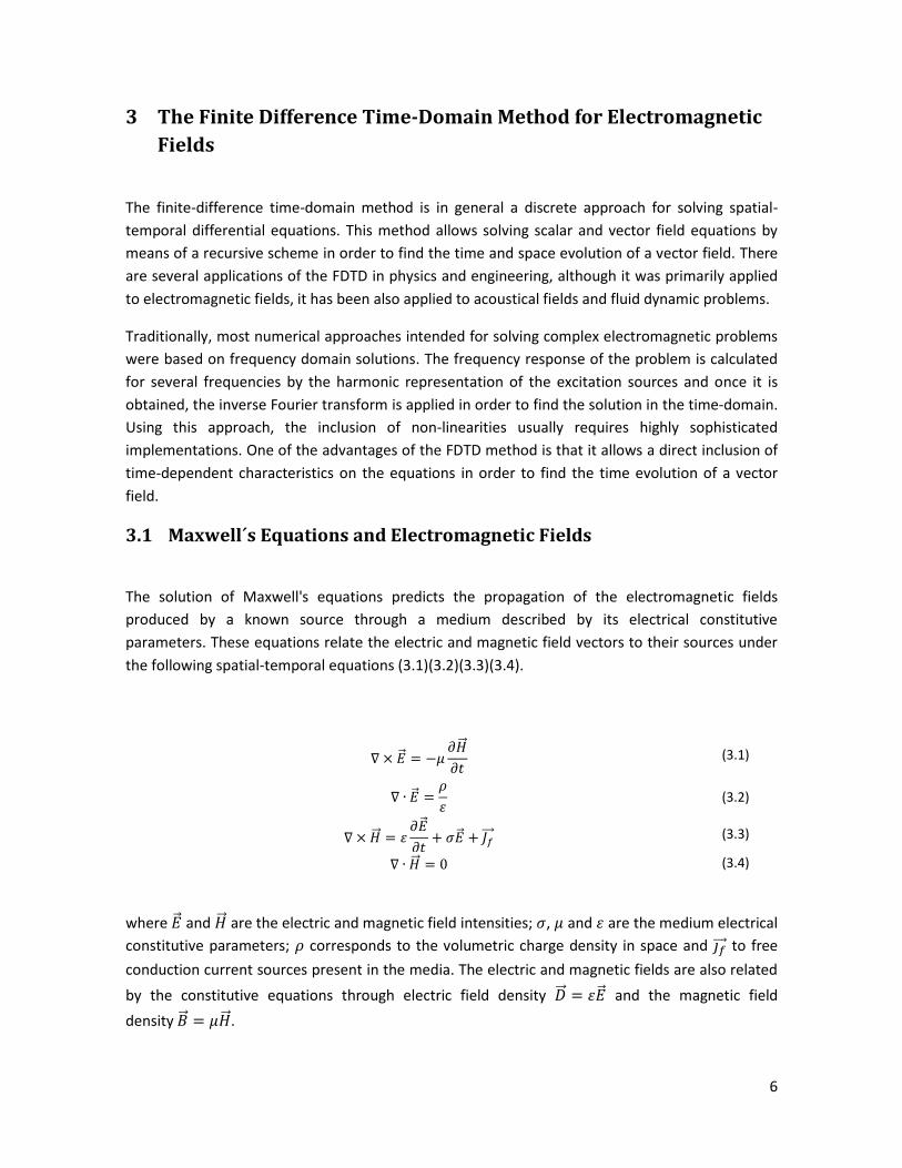
3.1 Maxwell´s Equations and Electromagnetic Fields
The solution of Maxwell's equations predicts the propagation of the electromagnetic fields
produced by a known source through a medium described by its electrical constitutive
parameters. These equations relate the electric and magnetic field vectors to their sources under
the following spatial-temporal equations (3.1)(3.2)(3.3)(3.4).
(3.1)
(3.2)
(3.3)
(3.4)
where and are the electric and magnetic field intensities; , and are the medium electrical
constitutive parameters; corresponds to the volumetric charge density in space and to free
conduction current sources present in the media. The electric and magnetic fields are also related
by the constitutive equations through electric field density and the magnetic field
density .

7
3.2 Numerical Solution of the Maxwell´s Equations
The finite-difference time-domain method is a discrete approach to the continuous
electromagnetic field formulation presented before, where the electric field components (Ex, Ey,
Ez) and the magnetic field components (Hx, Hy, Hz) are located in a staggered fashion over the faces
of a cube known as e Yee´s cell [28] as shown in Figure 1. The electrical constitutive parameters
are also discretized and related to each field component as ( , , ), ( , , ) and ( , ,
). Each cell representing a part of the space is related to a unique location (i, j, k) where i, j and k
are integers. These indexes are related to the actual coordinates of each field component, for
example, for the x-component of the magnetic field Hx the actual coordinates would be
( ) (( ) ( ) ( ) ) (3.5)
where and are the lengths of the cell sides.
(i, j, k)
Δx
Ex(i,j,k)
Hx(i,j,k)
x
yz
Ez(i,j+1,k)
Ey(i,j,k+1) Δy
Δz
Ey(i,j,k)
Ez(i,j,k)
Hz(i,j,k)
Figure 1 Yee's cell for the electric and magnetic fields location in space.
In vacuum, without any electric charge or current source, the set of equations (3.1)-(3.4) can be
reduced to (3.1) and (3.3) as the divergence equations are included in them [30]. When the
rotational equations are expanded using a Cartesian coordinate system, it is possible to obtain an
equation for the time variation of each component of the electromagnetic field as a function of
the spatial variation of its counterpart. This is shown in (3.6) for the x-component of the magnetic
field Hx.
(
) (3.6)
The side of the Yee’s cell relating the components of (3.6) is shown dotted in Figure 1. It can be
seen that (3.6) relates the time variation of the x-component of the magnetic field as a function of
the spatial variations of the electric fields components circulating around it; in this case the y and z
components of Ez and Ey. This distribution is adequate in order to apply a central-difference
approximation [30][31][32] to the terms on right hand side of (3.3) resulting in (3.7)
8
(
( ) ( )
( )
( )
) (3.7)
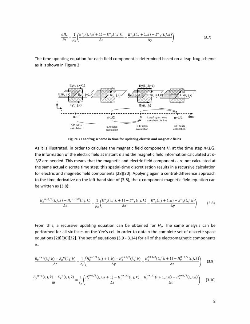
The time updating equation for each field component is determined based on a leap-frog scheme
as it is shown in Figure 2.
timen-1 n+1/2
B,H fields
calculation
D,E fields
calculation
Leapfrog scheme
calculation in time
Ey(i, j,k+1)
Hx(i, j,k)Ez(i, j,k) Hx(i, j,k)
Ey(i, j,k)
Ez(i, j+1,k)
Ey(i, j,k+1)
Ez(i, j,k)
Ey(i, j,k)
Ez(i, j+1,k)
n-1/2 n
D,E fields
calculation
B,H fields
calculation
y
z
Figure 2 Leapfrog scheme in time for updating electric and magnetic fields.
As it is illustrated, in order to calculate the magnetic field component Hx at the time step n+1/2,
the information of the electric field at instant n and the magnetic field information calculated at n-
1/2 are needed. This means that the magnetic and electric field components are not calculated at
the same actual discrete time step; this spatial-time discretization results in a recursive calculation
for electric and magnetic field components [28][30]. Applying again a central-difference approach
to the time derivative on the left-hand side of (3.6), the x-component magnetic field equation can
be written as (3.8):
( )
( )
(
( ) ( )
( )
( )
) (3.8)
From this, a recursive updating equation can be obtained for Hx. The same analysis can be
performed for all six faces on the Yee's cell in order to obtain the complete set of discrete-space
equations [28][30][32]. The set of equations (3.9 - 3.14) for all of the electromagnetic components
is:
( )
( )
(
( ) ( )
( )
( )
+ (3.9)
( )
( )
(
( ) ( )
( )
( )
+ (3.10)
9
( )
( )
(
( ) ( )
( )
( )
+ (3.11)
( )
( )
(
( ) ( )
( )
( )
) (3.12)
( )
( )
(
( ) ( )
( )
( )
) (3.13)
( )
( )
(
( ) ( )
( )
( )
) (3.14)
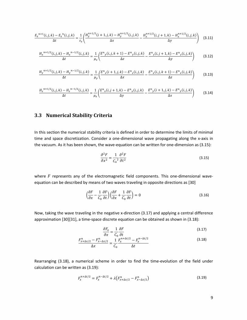
3.3 Numerical Stability Criteria
In this section the numerical stability criteria is defined in order to determine the limits of minimal
time and space discretization. Consider a one-dimensional wave propagating along the x-axis in
the vacuum. As it has been shown, the wave-equation can be written for one-dimension as (3.15):
(3.15)
where represents any of the electromagnetic field components. This one-dimensional wave-
equation can be described by means of two waves traveling in opposite directions as [30]
(
* (
* (3.16)
Now, taking the wave traveling in the negative x-direction (3.17) and applying a central difference
approximation [30][31], a time-space discrete equation can be obtained as shown in (3.18):
(3.17)
(3.18)
Rearranging (3.18), a numerical scheme in order to find the time-evolution of the field under
calculation can be written as (3.19):
(
) (3.19)

10
where, .
It can be shown that depending on the factor λ value, the recursive updating equation presented
above is stable if . Then,
(3.20)
The expression above allows defining the time-step value for stable calculations. Using an
attenuation factor, expression (3.20) can be written as (3.21)
(3.21)
where, is an attenuating factor used for maintaining a reasonable quantization error. The
same numerical stability condition can be found for the three dimensional wave equation as
[30][31][32]:
√
( )
( )
( )
(3.22)
If the spatial discretization is made by cubic cells the stability criteria can be
simplified to [31][32]:
√
(3.23)
where is the cell side length. In general, and it is typically set to be 0.9 for FDTD
simulations. This factor is known as the Courant’s factor. The relations that have been presented
here are illustrative, a more rigorous determination of the Courant’s factor can be found in [30].
3.4 Media Modeling
As the electrical constitutive parameters of the medium are directly related to their electric and
magnetic field components, the FDTD approach allows a straightforward inclusion of any material
and medium representation. As it was shown in section 3.2, the electrical constitutive parameters
are also discretized and related to each field component as ( , , ), ( , , ) and ( , ,
). In order to describe the constitutive parameter location into the Yee’s cube, some of the
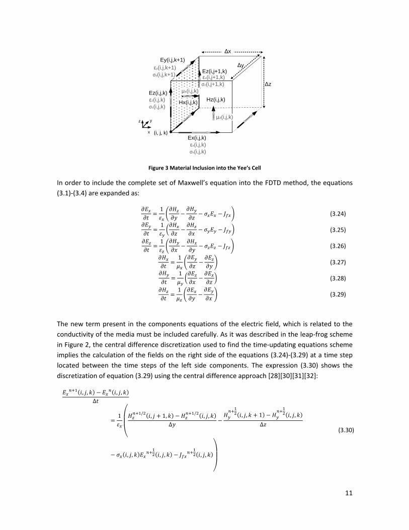
constitutive parameters components are shown in Figure 3.
11
εz(i,j+1,k)
σz(i,j+1,k)
(i, j, k)
Δx
Ex(i,j,k)
Hx(i,j,k)
x
yz
Ez(i,j+1,k)
Ey(i,j,k+1)Δy
Δz
Ez(i,j,k)
Hz(i,j,k)
μz(i,j,k)
μx(i,j,k)
εz(i,j,k)
σz(i,j,k)
εy(i,j,k+1)
σy(i,j,k+1)
εx(i,j,k)
σx(i,j,k)
Figure 3 Material Inclusion into the Yee’s Cell
In order to include the complete set of Maxwell’s equation into the FDTD method, the equations
(3.1)-(3.4) are expanded as:
(
) (3.24)
(
* (3.25)
(
) (3.26)
(
) (3.27)
(
* (3.28)
(
) (3.29)
The new term present in the components equations of the electric field, which is related to the
conductivity of the media must be included carefully. As it was described in the leap-frog scheme
in Figure 2, the central difference discretization used to find the time-updating equations scheme
implies the calculation of the fields on the right side of the equations (3.24)-(3.29) at a time step
located between the time steps of the left side components. The expression (3.30) shows the
discretization of equation (3.29) using the central difference approach [28][30][31][32]:
( )
( )
(
( ) ( )
( )
( )
( )
( )
( )
)
(3.30)

12
As the electric field component at the n+1/2 time step is not calculated by means of the time-
updating equation, an average of this electric field must be performed with those components
calculated at the n and n+1 time-steps as is shown in (3.31):
( )
( )
( )
(3.31)
Replacing (3.31) in (3.30) and rearranging some terms, a time-updating equation for the electric
field component under analysis can be found as is presented in (3.32). The time-updating
equations for the other electric field components can be found similarly [28][30][31][32]. As the
equations of the magnetic field components have not been modified by any new term, their time-
update equations remain unaltered as those presented in section 3.1.
( ) (
( ) ( )
( ) ( ))
( )
( ) ( )(
( ) ( )
+
( ) ( )(
( )
( )
,
( ) ( )
( )
(3.32)
As can be seen, the media parameter inclusion can be performed easily into the FDTD method if
the geometrical shape of the material coincides with a straight or parallelepipedal geometry. If this
is not the case, different techniques such as subcell models can be used in order to represent
curved geometrical features [30].
3.5 Lumped Elements Modeling
As it has been shown in the previous sections, the FDTD method uses a relation between the
electric and magnetic fields and the media parameters when they are located at specific places in
a cube cell. Based on this, it is possible to calculate the evolution in time of an electromagnetic
simulation scenario if the magnitude of any component of the electric or magnetic field is imposed
at some point. Lumped elements, such as sources, resistors, capacitors, inductors and non-linear
elements can be included into the FDTD method by means of the voltage-current relation between
their terminals. Equations (3.24) and (3.25) present the integral expression relating the voltage
and current magnitudes with the electric field and current density respectively [31].
Voltage and Electric Field relation Current and density Current relation
∫
(3.33) ∬
(3.34)

13
Any lumped component represented by means of it voltage-current relation can be included into
the FDTD scheme through the impressed current density term in the Ampère-Maxwell equation
(3.26):
(3.35)
Care must be taken as the voltage must be calculated in the same discrete time n as the electric
field, and the current must be also calculated as the same discrete time n+1/2 for the magnetic
field as:
(3.36)
(3.37)
Taking into account the equations (3.36) and (3.37) any voltage-current relation can be included
into the Yee´s cell and into the FDTD scheme in different convenient ways. Following subsections
show how to include different lumped elements such as sources and loads starting from their
voltage-current relation. All of the lumped elements that have been considered for illustration
have been placed in the z-direction.
3.5.1 Sources Modeling
Voltage and current sources are useful to model several electromagnetic problems, especially for
several engineering applications where the electromagnetic fields are generated by sophisticated
physical arrangements that depending on the simplifications and approximations, can be reduced
to this kind of representation. These elements can be included into the FDTD by means of the
imposition of a time-varying function on a component of the electric or magnetic field using the
physical relation between the fields and the voltage-current characteristic [30][31].
Consider a voltage source having an internal impedance different of zero placed between two z-
directed nodes of the Yee´s cube as is shown in Figure 4(a).
(i,j,k+1)
(i,j,k)
IV
-
+
∆Z
Rs
x
y
z
Vs(t) +-
(a)
(i,j,k+1)
(i,j,k)
V
-
+
∆Z
x
y
z
Is(t)
(b)
Figure 4 Source Modeling into the Yee´s Cell (a) Lumped Voltage Source with non-zero internal impedance (b) Current Source

14
The lumped voltage source can be related to the vertical electric field component between the
two nodes in the time domain by means of the expression:
( ) ( ) ( ) (3.38)
As it was explained before, the most convenient time-discretization for the expression (3.38) can
be written as:
(3.39)
As the current at the discrete instant n ( ) is not calculated explicitly in the recursive FDTD
scheme, its average is used:
(3.40)
Replacing (3.40) into (3.39) the expression for the voltage source with internal resistance can be
written as:
( )
(3.41)
Rearranging equation (3.41) and using (3.34), the lumped source expression can be written as:
(
) (3.42)
If the source to be modeled has zero internal resistance, then the voltage time-varying voltage
source into the FDTD method can be included as
(3.43)
In order to include a lumped current source, the expression (3.34) applied to a side of the Yee’s
cube leads to (3.44).
(3.44)
As it is shown in Figure 4(b) the current between the two nodes can be directly related to the
current density.
15
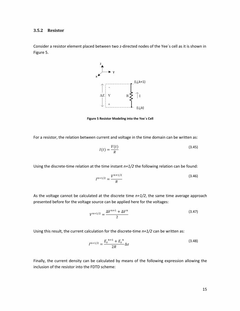
3.5.2 Resistor
Consider a resistor element placed between two z-directed nodes of the Yee´s cell as it is shown in
Figure 5.
(i,j,k+1)
(i,j,k)
IV
-
+
∆Z R
x
y
z
Figure 5 Resistor Modeling into the Yee´s Cell
For a resistor, the relation between current and voltage in the time domain can be written as:
( ) ( )
(3.45)
Using the discrete-time relation at the time instant n+1/2 the following relation can be found:
(3.46)
As the voltage cannot be calculated at the discrete time n+1/2, the same time average approach
presented before for the voltage source can be applied here for the voltages:
(3.47)
Using this result, the current calculation for the discrete-time n+1/2 can be written as:
(3.48)
Finally, the current density can be calculated by means of the following expression allowing the
inclusion of the resistor into the FDTD scheme:
16
[
]
(3.49)
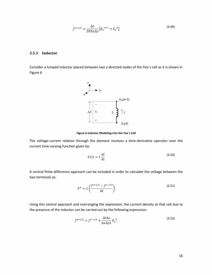
3.5.3 Inductor
Consider a lumped inductor placed between two z-directed nodes of the Yee´s cell as it is shown in
Figure 6
(i,j,k+1)
(i,j,k)
IV
-
+
∆Z L
x
y
z
Figure 6 Inductor Modeling into the Yee´s Cell
The voltage-current relation through the element involves a time-derivative operator over the
current time-varying function given by:
( )
(3.50)
A central finite-difference approach can be included in order to calculate the voltage between the
two terminals as:
(
)
(3.51)
Using this central approach and rearranging the expression, the current density at that cell due to
the presence of the inductor can be carried out by the following expression:
(3.52)
17
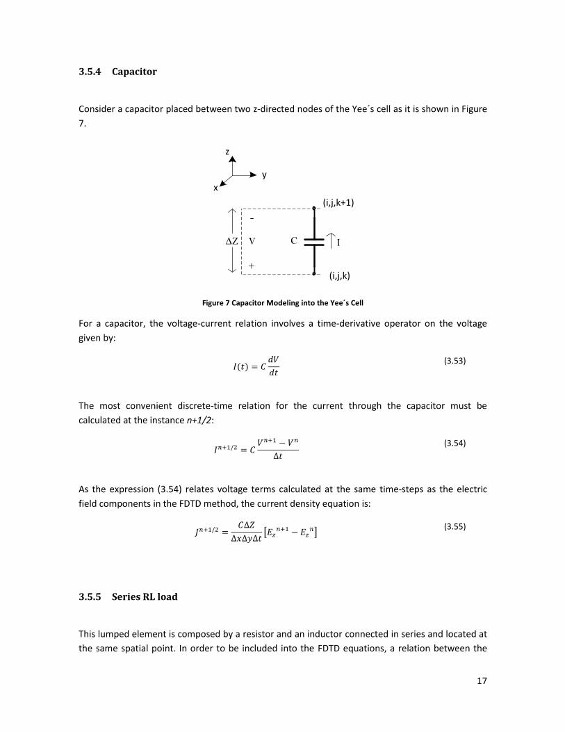
3.5.4 Capacitor
Consider a capacitor placed between two z-directed nodes of the Yee´s cell as it is shown in Figure
7.
(i,j,k+1)
(i,j,k)
IV
-
+
∆Z C
x
y
z
Figure 7 Capacitor Modeling into the Yee´s Cell
For a capacitor, the voltage-current relation involves a time-derivative operator on the voltage
given by:
( )
(3.53)
The most convenient discrete-time relation for the current through the capacitor must be
calculated at the instance n+1/2:
(3.54)
As the expression (3.54) relates voltage terms calculated at the same time-steps as the electric
field components in the FDTD method, the current density equation is:
[
]
(3.55)
3.5.5 Series RL load
This lumped element is composed by a resistor and an inductor connected in series and located at
the same spatial point. In order to be included into the FDTD equations, a relation between the

18
electric and magnetic fields must take into account the effect of the series inductive and resistive
load. Consider a lumped resistor in series with an inductor placed between two z-directed nodes
of the Yee´s cell as it is shown in Figure 8.
(i,j,k+1)
(i,j,k)
IV
-
+
∆Z
L
x
y
z
R
Figure 8 Lumped RL-Load Modeling into the Yee´s Cell
The equation that relates the voltage and current for the series RL-lumped element can be written
as:
( ) ( )
(3.56)
In order to include the series RL-lumped element into the FDTD scheme, the discretization can be
done as it was presented for the resistor and the inductor. The most convenient formulation can
be written as:
(
) (
)
(3.57)
Using the expression for the voltage calculation by means of the electric field and rearranging
expression (3.57), it can be obtained (3.58):
( )
( )
( )
(3.58)
Finally, using equation (3.58) and expressing in terms of the current-density, it can be shown:
( )
( )
( )
(3.59)
19
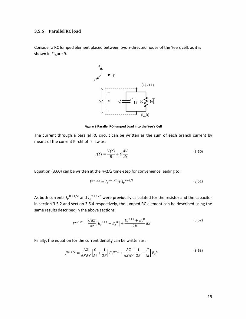
3.5.6 Parallel RC load
Consider a RC lumped element placed between two z-directed nodes of the Yee´s cell, as it is
shown in Figure 9.
(i,j,k+1)
(i,j,k)
I2V
-
+
∆Z C R
x
y
z
I1
Figure 9 Parallel RC-lumped Load into the Yee´s Cell
The current through a parallel RC circuit can be written as the sum of each branch current by
means of the current Kirchhoff’s law as:
( ) ( )
(3.60)
Equation (3.60) can be written at the n+1/2 time-step for convenience leading to:
(3.61)
As both currents and
were previously calculated for the resistor and the capacitor
in section 3.5.2 and section 3.5.4 respectively, the lumped RC element can be described using the
same results described in the above sections:
[
]
(3.62)
Finally, the equation for the current density can be written as:
[
]
[
]
(3.63)
20
3.6 Boundary Conditions
As it has been presented above, the FDTD method produces a recursive scheme for calculating
magnetic and electric field including not only the material properties but also different lumped
elements. The relations derived before have been presented for a general discrete point (i,j,k)
inside the problem space.
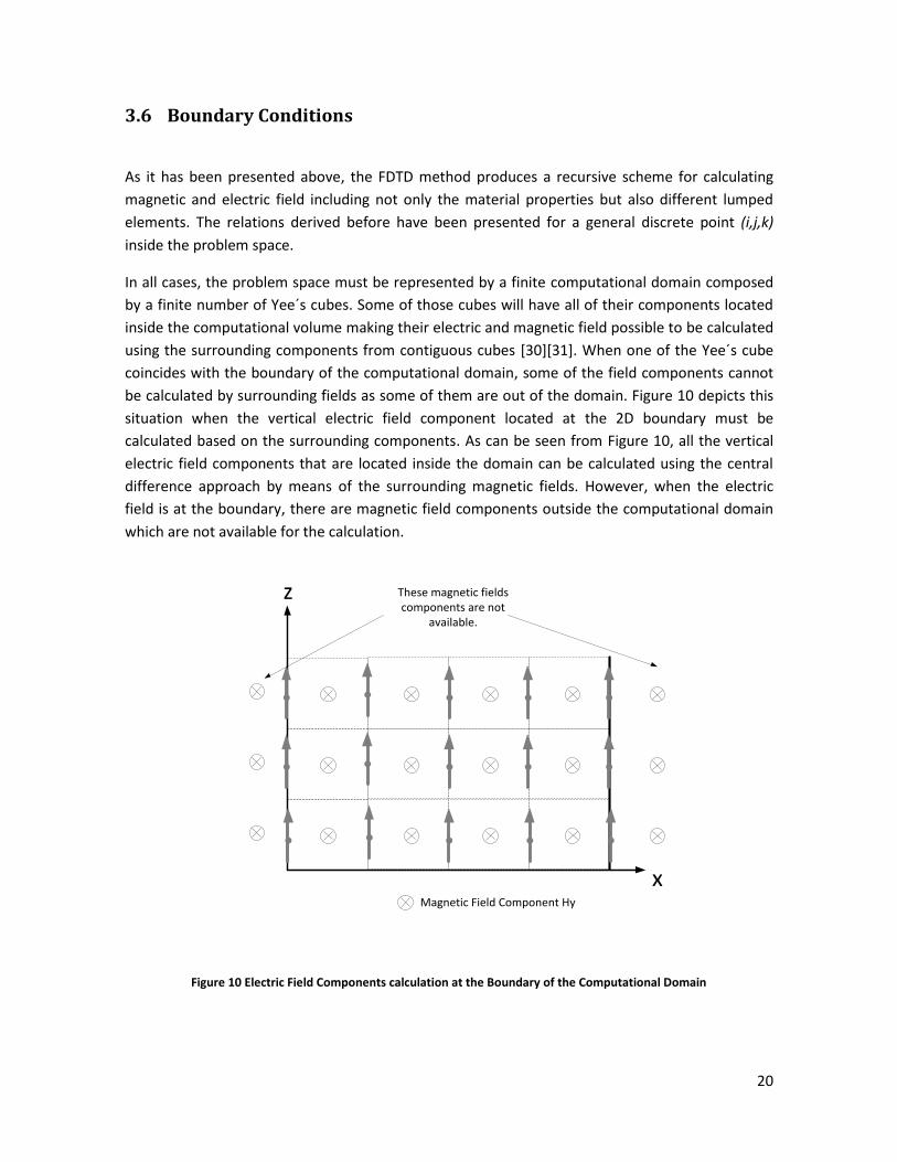
In all cases, the problem space must be represented by a finite computational domain composed
by a finite number of Yee´s cubes. Some of those cubes will have all of their components located
inside the computational volume making their electric and magnetic field possible to be calculated
using the surrounding components from contiguous cubes [30][31]. When one of the Yee´s cube
coincides with the boundary of the computational domain, some of the field components cannot
be calculated by surrounding fields as some of them are out of the domain. Figure 10 depicts this
situation when the vertical electric field component located at the 2D boundary must be
calculated based on the surrounding components. As can be seen from Figure 10, all the vertical
electric field components that are located inside the domain can be calculated using the central
difference approach by means of the surrounding magnetic fields. However, when the electric
field is at the boundary, there are magnetic field components outside the computational domain
which are not available for the calculation.
x
z
Magnetic Field Component Hy
These magnetic fields components are not
available.
Figure 10 Electric Field Components calculation at the Boundary of the Computational Domain

21
In order to overcome this problem, several methods have been proposed in literature for
calculating the components of the electromagnetic field at the boundary based on its past values
and available components located inside the domain. Typically, the boundary conditions are
applied to the electric field components because they can be easily related to physical conditions
(i.e. when perfectly conductive planes are present). However, boundary conditions can be also
applied for magnetic field components placed on the boundary [30]. In this thesis all the
boundaries conditions were implemented for the electric field components.
3.6.1 Perfectly Conductive Boundary Condition
This boundary condition assumes that the boundaries of the computational domain are perfect
conductors with zero thickness [28][30][31]. This assumption allows defining the electric field
components as inside a perfect conductor, therefore they are forced to be zero. These boundaries
are commonly named as Perfect Electric Conductor or “PEC” Boundaries.
A computational set up was proposed in order to evaluate the PEC implementation into the FDTD
scheme. The total domain was simulated using 50x24x10 cubic cells; each cube was simulated with
a side of 2mm in length. The source was represented by means of an array of vertical electric field
components with the same waveform; it is worth noting that all of the sources were imposed with
no phase delay between each other in order to control the symmetry of the radiated wave
propagation. The vertical source array was placed at (26, 13) on the XY plane and extended along
the Z axis; the electric field measured was located at the node (33, 13, 5). Figure 11(a) presents the
simulation set-up.
x
y
z
PEC
PEC
source array of Vertical Electric Field Components
All PEC Boundaries
24 cells
10 cells
50 cells
Receiver Point
(a) (b)
0 0.2 0.4 0.6 0.8 1-10
-5
0
5
10
Time [ns]
Ele
ctr
ic F
ield
Ez [
V/m
]

22
(c) (d)
Figure 11 (a) Simulation Set-up for PEC Boundaries Implementation (b) Source Waveform (c) Electric Field Magnitudes for each component at the Receiver Point (d) Magnetic Field magnitudes for each component at the Receiver Point
Figure 11(b) shows the source waveform used in the simulation set-up. This waveform known as
the normalized derivative Gaussian waveform and is commonly used for the excitation of a wide
frequency spectrum without taking into account very low frequency components [31].
Despite the excitation vanishes once the bipolar pulse ends, the electromagnetic field components
showed in Figure 11(c) and Figure 11(d) present an oscillatory pattern for the entire time interval.
These patterns are caused by the multiple reflections of the electromagnetic wave on the
boundaries. An infinite oscillatory steady-state will be reached and most of the resonance
characteristics of the cavity can be analyzed from the time solution.
3.6.2 Absorbing Boundaries Conditions
PEC boundaries are useful when perfectly conductive thin layers must be included into the
simulation. However, several applications require that the boundaries act as an open space,
meaning that no reflections of the incident waves are desired. This section presents some of the
most popular boundary conditions that have been proposed in literature for non-reflecting
characteristics at the boundary of the computational domain. All of these boundaries are based on
known values taken from the internal domain, leading to a set of updating equations for the
electric field components at the boundary.
3.6.2.1 Mur´s Boundaries
The Mur´s Boundaries conditions are based on the plane-wave unbounded propagation
characteristics [33]. The wave equation for any component of the electromagnetic field can be
written as:
(3.64)
0 0.2 0.4 0.6 0.8 1-1
-0.5
0
0.5
1
Time [ns]
Ele
ctr
ic F
ield
[V
/m]
Ex
Ey
Ez
0 0.2 0.4 0.6 0.8 1-2
0
2
4
Time [ns]
Magnetic F
ield
[m
A/m
]
Hx
Hy
Hz
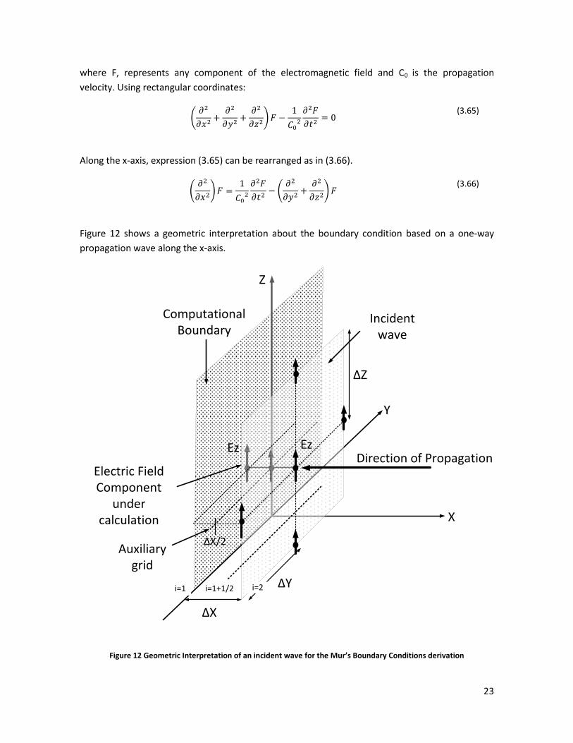
23
where F, represents any component of the electromagnetic field and C0 is the propagation
velocity. Using rectangular coordinates:
(
)
(3.65)
Along the x-axis, expression (3.65) can be rearranged as in (3.66).
(
)
(
)
(3.66)
Figure 12 shows a geometric interpretation about the boundary condition based on a one-way
propagation wave along the x-axis.
X
Z
Y
Ez
∆X
∆Y
∆Z
Incident wave
Computational Boundary
Direction of PropagationEz
Electric Field Component
under calculation
Auxiliary grid
∆X/2
i=1 i=1+1/2 i=2
Figure 12 Geometric Interpretation of an incident wave for the Mur’s Boundary Conditions derivation

24
From Figure 12, an area ∆Y∆Z is taken into account as a part of the wave front reaching the
boundary. The vertical electric field component at the boundary can be related to the spatial
variation of the field on the wave front segment and its time variation, by means of the expression
(3.66) evaluated at the auxiliary grid located at ∆X/2.
In order to obtain an explicit time-updating equation for the components at the boundary,
expression (3.66) can be rearranged as:
(
)
(
(
,
)
(3.67)
Defining,
(
,
(3.68)
and replacing (3.68) in (3.67) yields to:
(
)
(
( )+
(3.69)
By means of the derivative operator properties, the wave equation can be factorized as [30]:
(
√ * (
√ *
(3.70)
The boundary condition now can be applied depending on the direction of the incident wave. If
the field component in the x-direction is assumed to be a plane unidirectional wave traveling in
the negative direction of the x-axis, the boundary condition can be calculated for the left term of
the equation above as:
(
√ *
(3.71)
The imperfection of the absorbing characteristics rises from the discretization of equation (3.71).
Engquist and Majda [34] proposed an expansion of the √ term using Taylor series and
leading to different approximations for the numerical simulation of incident waves depending on
the number of terms taken into account [30].
Mur, proposed a discrete approach for equation (3.71) and a Taylor series representation based
on a finite central difference approximation, in order to represent the boundary condition using
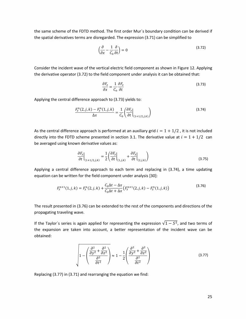
25
the same scheme of the FDTD method. The first order Mur´s boundary condition can be derived if
the spatial derivatives terms are disregarded. The expression (3.71) can be simplified to
(
*
(3.72)
Consider the incident wave of the vertical electric field component as shown in Figure 12. Applying
the derivative operator (3.72) to the field component under analysis it can be obtained that:
(3.73)
Applying the central difference approach to (3.73) yields to:
( )
( )
(
|( )
) (3.74)
As the central difference approach is performed at an auxiliary grid , it is not included
directly into the FDTD scheme presented in section 3.1. The derivative value at can
be averaged using known derivative values as:
|( )
(
|( )
|( )
)
(3.75)
Applying a central difference approach to each term and replacing in (3.74), a time updating
equation can be written for the field component under analysis [30]:
( )
( )
(
( ) ( ))
(3.76)
The result presented in (3.76) can be extended to the rest of the components and directions of the
propagating traveling wave.
If the Taylor´s series is again applied for representing the expression √ , and two terms of
the expansion are taken into account, a better representation of the incident wave can be
obtained:
√ (
,
(
, (3.77)
Replacing (3.77) in (3.71) and rearranging the equation we find:

26
(
)
(3.78)
Using a central difference approach for discretizing the differential equation in space and time, the
second order Mur’s boundaries can be found. For this case the discretization leads to a second
order derivative discrete equation. Again, the central difference approach is used at the auxiliary
grid presented in Figure 12. As the auxiliary grid is not explicit in the FDTD scheme presented in
section 3.1, the second order time derivative can be calculated as an average between the time
derivative of the adjacent points (3.80) and for the space-second order derivatives (3.81)-(3.82):
|( )
(
*
(
|( )
|( )
) (3.79)
|( )
(
|( )
|( )
+ (3.80)
|( )
(
|( )
|( )
+ (3.81)
|( )
(
|( )
|( )
+ (3.82)
Applying the central differences and replacing in (3.78), an expression for the unknown field at the
boundary can be found in function of the inner field values as [30][33]:
( )
( )
(
( ) ( ))
(
( ) ( ))
( )
( )(
( )
( ) ( )
( )
( ) ( )
*
( )
( )(
( )
( ) ( )
( )
( ) ( )
*
(3.83)
The expression presented in (3.83) can be also derived for the remaining components. In order to
validate the implementation of the Mur´s boundaries in the FDTD formulation presented in this
thesis, Figure 13 shows the comparison between the results obtained by the implementation of
the Mur’s boundaries in this thesis with those results presented in [33]. The simulation set-up
consisted of a vertical current dipole with a harmonic excitation of wavelength λ. The current
dipole was located at the coordinate (5λ, 5λ) on the XY plane. A contour plot of this field
component is obtained from XY plane values.

27
(a)
(b) Figure 13 Vertical Electric Field contour plot of an oscillating vertical current dipole by using Mur’s Boundaries as ABCs (a) Contour Radiation Pattern for the first Order and second order approximation presented in [33] (b) 1st Order and
2nd
Order Mur’s Boundaries implementation
As the results presented in [33] were obtained from a 2D implementation of the FDTD method,
and the implementation made in this thesis was extended to the 3D full wave solution, some
slightly differences between both results are present. It can be seen that using the Mur’s
boundaries, the expected behavior of the electric field of a typical vertical dipole can be well
reproduced by the proposed expressions for the truncation of the computational domain. It can be
also seen that the second order representation of the boundary conditions improves enormously
the radiation contour plot when they are compared to the first order approach.
3.6.2.2 Liao´s Boundaries
The Liao´s boundaries are one of the most simple and effective absorbing boundary conditions
presented in the literature. They were proposed in 1984 by Liao et al [35]. The idea behind the
Liao’s proposal is to obtain the electric field components at the boundary by means of an
extrapolation of the internal electric field values. These boundaries are based on the wave
propagation characteristics as it was proposed by Mur [33]. However, the fields at the boundary
are calculated based on the past values of the fields using a polynomial expression. Figure 14
presents an interpretation of the Liao´s extrapolation for a one-dimensional propagating wave.
0.1
[p.u
]
0.1 [p.u]
10
20
30
10 20 30
Mur's 1st Order ABC
Mur's 2nd Order ABC
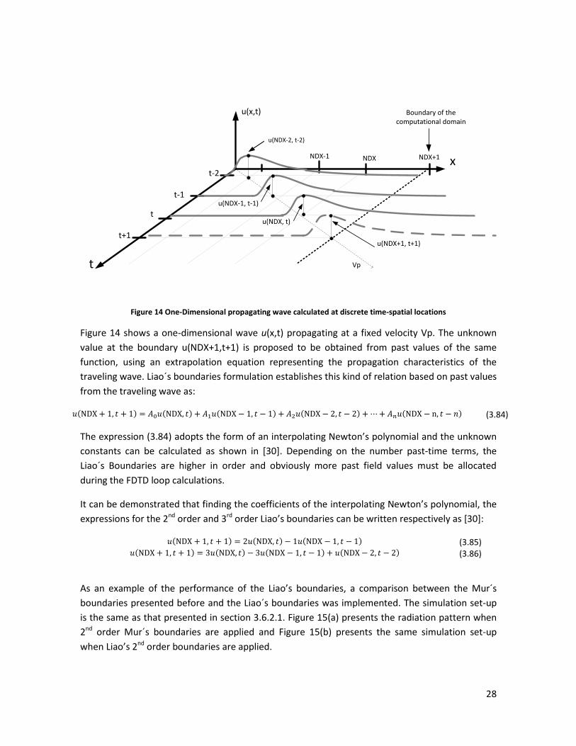
28
NDX-1
t
x
u(x,t)
t+1
t
t-1
t-2
u(NDX-1, t-1)
u(NDX-2, t-2)
NDX+1NDX
u(NDX+1, t+1)
u(NDX, t)
Boundary of the computational domain
Vp
Figure 14 One-Dimensional propagating wave calculated at discrete time-spatial locations
Figure 14 shows a one-dimensional wave u(x,t) propagating at a fixed velocity Vp. The unknown
value at the boundary u(NDX+1,t+1) is proposed to be obtained from past values of the same
function, using an extrapolation equation representing the propagation characteristics of the
traveling wave. Liao´s boundaries formulation establishes this kind of relation based on past values
from the traveling wave as:
( ) ( ) ( ) ( ) ( )
(3.84)
The expression (3.84) adopts the form of an interpolating Newton’s polynomial and the unknown
constants can be calculated as shown in [30]. Depending on the number past-time terms, the
Liao´s Boundaries are higher in order and obviously more past field values must be allocated
during the FDTD loop calculations.
It can be demonstrated that finding the coefficients of the interpolating Newton’s polynomial, the
expressions for the 2nd order and 3rd order Liao’s boundaries can be written respectively as [30]:
( ) ( ) ( ) (3.85) ( ) ( ) ( ) ( ) (3.86)
As an example of the performance of the Liao’s boundaries, a comparison between the Mur´s
boundaries presented before and the Liao´s boundaries was implemented. The simulation set-up
is the same as that presented in section 3.6.2.1. Figure 15(a) presents the radiation pattern when
2nd order Mur´s boundaries are applied and Figure 15(b) presents the same simulation set-up
when Liao’s 2nd order boundaries are applied.

29
(a)
(b)
(c)
Figure 15 Liao´s Boundaries performance compared with (a) Mur´s Boundaries (2nd
Order) Boundaries (b) Liao’s Boundaries (2
nd Order) (c) Contour plot comparison
As can be seen from Figure 15(c), Liao’s boundaries present a better performance for the expected
cylindrical pattern. Due to this, Liao’s boundaries have become one of the most used absorbing
boundaries not only by its good performance, but also by its straightforward implementation
when compared with other sophisticated absorbing boundary conditions. Liao´s boundaries has
been tested in several numeric experiments and it has been shown a good absorbing condition
and low sensitivity to the incident wave propagating angle. These boundaries present between
10dB and 20dB less reflection than the 2nd order Mur’s boundaries [30].
0.1
[p.u
]
0.1 [p.u]
-20
-20
-20
-20
-20
-20
-20
-20
-20
-20
-20
-20-20
-20
-20
-20
-20
-20
-20
-20
-15
-15
-15
-15
-15
-15
-15
-15
-15
-15
-15
-15
-15
-15
-15
-15-1
5
-15
-15
-15
-15
-15
1212
12
12
12
12
12
12
12
12
12
12
12
12
12
12
12
12 1
2
12
12
12
12
30
3030
30
30
3030
30
30
3030
10
20
30
10 20 30
-20-20
-20
-20
-20
-20
-20
-20
-20
-20
-20
-20
-20
-20
-20
-20
-20
-20
-20
-20
-20
-20
-20
-20
-20
-15
-15
-15
-15
-15
-15
-15
-15
-15
-15
-15
-15
-15
-15
-15
-15
-15
-15
-15
-15
-15
-15
-15
-15
12
12
12
12
12
12
12
12
12
12
12
12
1212
12
12
12
12
12
12
12
12
12
30
30
30
30
30
30
30
30
30
30
30
30
30
0.1
[p
.u]
0.1 [p.u]
10
20
30
10 20 30
0.1
[p.u
]
0.1 [p.u]
10
20
30
10 20 30
Mur's ABCs
Liao's ABCs

30
3.6.3 PML and CPML Boundaries
One of the most effective implementation for absorbing boundaries is that proposed by Berenger
in 1994 [36]. This approach is based on the idea of truncating the computational domain by means
of an artificial medium with the same electromagnetic propagation characteristics of the medium
in which an electromagnetic wave is propagating through. This has the mathematical consequence
of non-reflections from the truncating medium. The Perfectly Matched Layer - PML absorbing
boundary condition can theoretically perfectly match any type of medium [36]. Depending on the
implementation and the discretization of the equations, some numerical reflections can occur.
However, it has been shown that the reflections due to the PML implementation are far lower
than other absorbing boundaries approaches [30][36].
The implementation of the PML into the FDTD method has been very popular and its better
performance as an absorbing boundary condition has been widely demonstrated [30][31][36][37].
The Convolutional Perfect Matched Layer (CPML) is an improvement of the PML boundary
condition [31][39].
Figure 16 presents a comparison of the performance between the CPML boundaries and the
implementations of boundary conditions that have been analyzed before in this thesis. The results
presented for the CPML boundary conditions were obtained by using the formulation discussed in
[31].
The simulation setup was composed of a vertical electric dipole represented by a voltage source
with a 50Ω internal resistance. The total problem space was 50 x 50 x 50m3 and the discretization
was performed using cubic Yee´s cells with 1m3 in volume. The source was placed at the center of
the problem space volume and the observation point was located at the coordinate (X=10.5m,
Y=10.5m, and Z=10.5m). The voltage source excitation was set to be a Gaussian’s pulse described
by the expression:
( )
( )
(3.87)
The parameters were set to and [31].Figure 16(a) presents the excitation waveform.
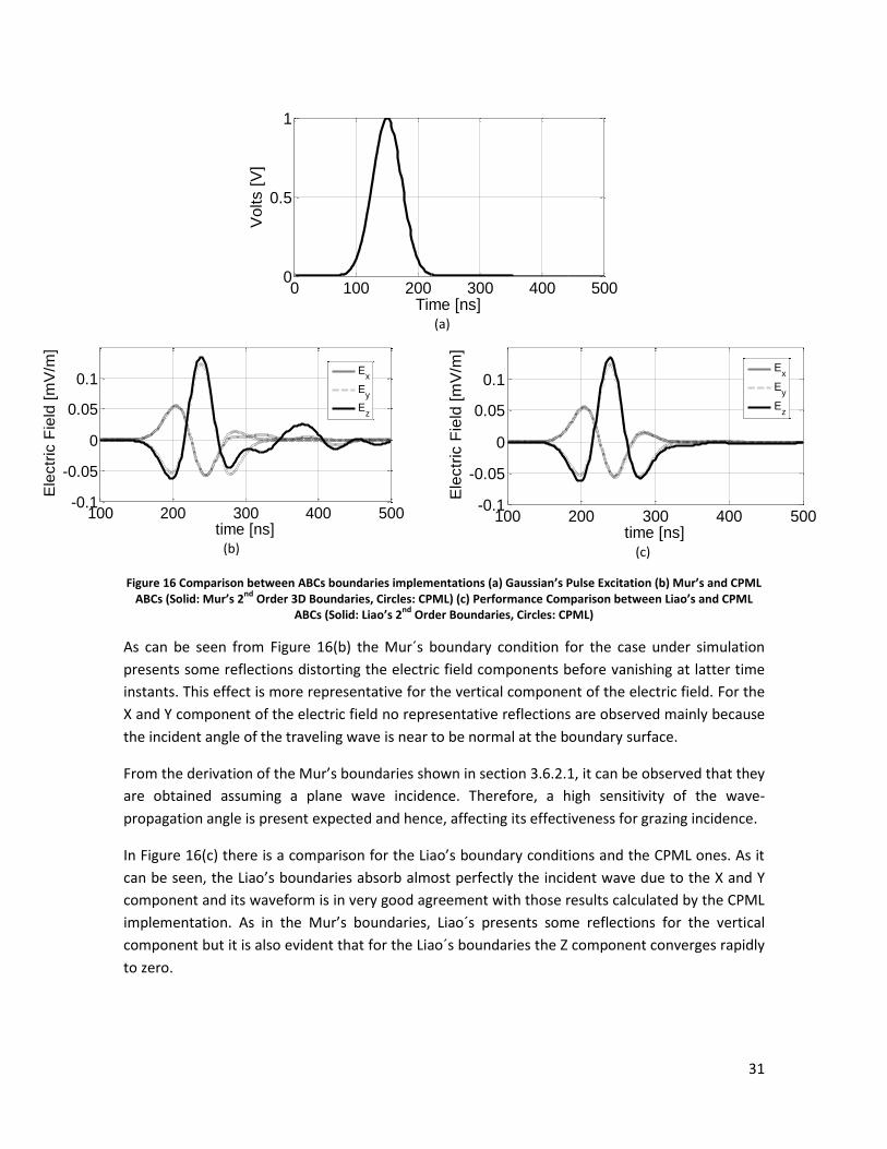
31
(a)
(b)
(c)
Figure 16 Comparison between ABCs boundaries implementations (a) Gaussian’s Pulse Excitation (b) Mur’s and CPML ABCs (Solid: Mur’s 2
nd Order 3D Boundaries, Circles: CPML) (c) Performance Comparison between Liao’s and CPML
ABCs (Solid: Liao’s 2nd
Order Boundaries, Circles: CPML)
As can be seen from Figure 16(b) the Mur´s boundary condition for the case under simulation
presents some reflections distorting the electric field components before vanishing at latter time
instants. This effect is more representative for the vertical component of the electric field. For the
X and Y component of the electric field no representative reflections are observed mainly because
the incident angle of the traveling wave is near to be normal at the boundary surface.
From the derivation of the Mur’s boundaries shown in section 3.6.2.1, it can be observed that they
are obtained assuming a plane wave incidence. Therefore, a high sensitivity of the wave-
propagation angle is present expected and hence, affecting its effectiveness for grazing incidence.
In Figure 16(c) there is a comparison for the Liao’s boundary conditions and the CPML ones. As it
can be seen, the Liao’s boundaries absorb almost perfectly the incident wave due to the X and Y
component and its waveform is in very good agreement with those results calculated by the CPML
implementation. As in the Mur’s boundaries, Liao´s presents some reflections for the vertical
component but it is also evident that for the Liao´s boundaries the Z component converges rapidly
to zero.
0 100 200 300 400 5000
0.5
1
Time [ns]
Volts [
V]
100 200 300 400 500-0.1
-0.05
0
0.05
0.1
time [ns]
Ele
ctr
ic F
ield
[m
V/m
]
Ex
Ey
Ez
100 200 300 400 500-0.1
-0.05
0
0.05
0.1
time [ns]
Ele
ctr
ic F
ield
[m
V/m
]
Ex
Ey
Ez
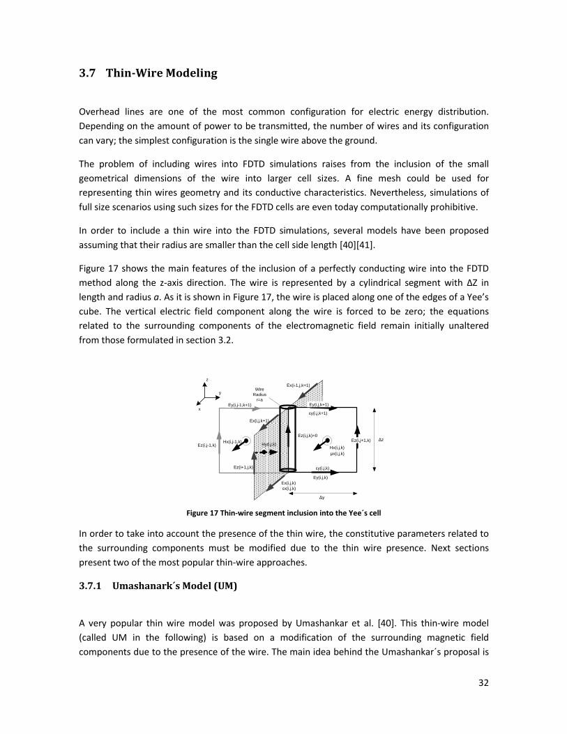
32
3.7 Thin-Wire Modeling
Overhead lines are one of the most common configuration for electric energy distribution.
Depending on the amount of power to be transmitted, the number of wires and its configuration
can vary; the simplest configuration is the single wire above the ground.
The problem of including wires into FDTD simulations raises from the inclusion of the small
geometrical dimensions of the wire into larger cell sizes. A fine mesh could be used for
representing thin wires geometry and its conductive characteristics. Nevertheless, simulations of
full size scenarios using such sizes for the FDTD cells are even today computationally prohibitive.
In order to include a thin wire into the FDTD simulations, several models have been proposed
assuming that their radius are smaller than the cell side length [40][41].
Figure 17 shows the main features of the inclusion of a perfectly conducting wire into the FDTD
method along the z-axis direction. The wire is represented by a cylindrical segment with ΔZ in
length and radius a. As it is shown in Figure 17, the wire is placed along one of the edges of a Yee’s
cube. The vertical electric field component along the wire is forced to be zero; the equations
related to the surrounding components of the electromagnetic field remain initially unaltered
from those formulated in section 3.2.
Ez(i,j,k)=0Ez(i,j+1,k)
Ey(i,j,k)
Ey(i,j,k+1)
Ez(i+1,j,k)
Ex(i,j,k+1)
Ex(i,j,k)
Hx(i,j,k)Hy(i,j,k)
Wire
Radius
r=a
Δy
Δz
εy(i,j,k+1)
εy(i,j,k)
εx(i,j,k)
μx(i,j,k)
Ez(i,j-1,k)
Ex(i-1,j,k+1)
Ey(i,j-1,k+1)
Hx(i,j-1,k)
y
x
z
Figure 17 Thin-wire segment inclusion into the Yee´s cell
In order to take into account the presence of the thin wire, the constitutive parameters related to
the surrounding components must be modified due to the thin wire presence. Next sections
present two of the most popular thin-wire approaches.
3.7.1 Umashanark´s Model (UM)
A very popular thin wire model was proposed by Umashankar et al. [40]. This thin-wire model
(called UM in the following) is based on a modification of the surrounding magnetic field
components due to the presence of the wire. The main idea behind the Umashankar´s proposal is

33
to find the surrounding magnetic field by means of the Faraday´s law equation assuming an
electrostatic and magnetostatic behavior of the fields near the wire[30][31][40]. In Figure 18 there
is a representation of a vertical segment of a straight wire.
Ez(x,y,z+Δz/2,t)=0
Ey(x,∆y/2,z+Δz,t)
WireRadius r
Δz
y
x
z
Δy/2
Ez(x,y+∆y,z+Δz/2,t)
Hx(x,∆y/2,z+Δz/2,t)
Faraday´s law must be satisfied
in this area
z
z+Δz
(x,y,z)
(x,y,z+Δz)
Ey(x,∆y/2,z,t)
Figure 18 Segment of a z-directed wire
Applying the Faraday´s law on the shadowed area, the components of the fields can be related
each other as:
∬
∬
(3.88)
Using the Stokes´ theorem in (3.88) a relation between the magnetic field on the area of interest
and the surrounding electric fields can be obtained:
∮
∬
(3.89)
Assuming static electric and magnetic fields distributions in the vicinity the wire, their components
can be expressed as inverse-distance dependent from the wire axis, as:
( )
| ( )
(3.90)
( )
| ( )
(3.91)
( )
( )
(3.92)
where | ( ) , |
( ) and ( ) are a unknown time-dependent functions evaluated at
the locations depicted in Figure 18. Including them into (3.89) it can be obtained:

34
∫ ( |
+
( ) ∫ ( |
+
( ∬
) (3.93)
Integrating (3.93) and rearranging some terms,
* | | + (
* ( ) (
*
(3.94)
Evaluating the fields at the locations presented in Figure 18, it can be found that:
| ( ) (
* (
* (3.95)
| ( ) (
* (
* (3.96)
( ) (
* (
* (3.97)
Replacing (3.95), (3.96) and (3.97) in (3.94) yields finally to:
(
* (
* (
)
[(
* (
* (
* (
*] (
* ( )
(3.98)
Rearranging terms in the (3.98) it is possible to obtain:
(
)
(
) ( )
[ (
* (
*]
(3.99)
Figure 19 presents the inclusion of a vertical thin-wire segment between the nodes (i,j,k) and
(i,j,k+1) using the same indexes notation as in section 3.2. It is worth noting that the location of
the components coincides with those obtained from the Umashankar’s method but in this case for
a general location point (i,j,k) in the discrete computational domain in order to use the FDTD
scheme for the time-space discretization [31][40].

35
Ez(i,j,k)=0Ez(i,j+1,k)
Ey(i,j,k)
Ey(i,j,k+1)
Ez(i+1,j,k)
Ex(i,j,k+1)
Ex(i,j,k)
Hx(i,j,k)Hy(i,j,k)
WireRadius r
Δy
Δz
εy(i,j,k+1)
εy(i,j,k)
εx(i,j,k)
μx(i,j,k)
Ez(i,j-1,k)
Ex(i-1,j,k+1)
Ey(i,j-1,k+1)
Hx(i,j-1,k)
y
x
z
Figure 19 Thin-wire inclusion in the Yee´s cube
In order to discretize (3.99) and include it into the FDTD scheme, the time-updating equations for
the magnetic fields presented in section 3.1 and section 3.4 must be modified for all magnetic
components surrounding the wire. The discrete time-updating equation for the magnetic fields
components around the wire shown in Figure 19, can be found applying the central difference
approach to (3.99) leading to:
( )
( )
( ) (
)
( )
( ) [
( ) ( )]
(3.100)
The UM model has been useful for the calculation of the radiated fields from an antenna; however
its accuracy decreases for surge impedance calculations [40][41].
3.7.2 Noda-Yokoyamas’s Model (NY)
As it was presented in the previous section, the thin-wire is included into the FDTD scheme
modifying the time-updating equations for the magnetic field components around the wire. Noda
and Yokoyama proposed a thin-wire model (NY) based on the concept of the intrinsic radius [41].
In this model, the electric field component along the wire is also forced to be zero in order to
satisfy the perfectly conductive condition inside the wire. Besides, this model modifies not only
the surrounding magnetic field components but also the electric field ones.
The NY thin-wire representation assumes an artificial wire with radius ro surrounded by a modified
media characterized by its electric permittivity and magnetic permeability, in order to reproduce
the electric and magnetic field distributions around the actual wire. This artificial radius is called
the intrinsic radius. The correction factor m applied to the electric permittivity and magnetic
permeability around the artificial wire, can be found by equating the electrostatic distribution due
to the actual wire to the distribution produced by the artificial wire. According to this, the
correction factor can be calculated from [41]:

36
(
)
(3.101)
where is the side length as it is shown in Figure 20. Once the correction factor is calculated, the
modified permittivity and the modified permeability around the wire can be obtained from
(3.102) and (3.103) respectively.
(3.102) (3.103)
Figure 20 presents the permittivity and permeability components around the wire that must be
modified by the factor m calculated in (3.101). These components have been highlighted in the
figure.
Ez(i,j,k)=0 Ez(i,j+1,k)
Ey(i,j,k)
Ey(i,j,k+1)
Ez(i+1,j,k)
Ex(i,j,k+1)
Ex(i,j,k)
Hx(i,j,k)Hy(i,j,k)
WireRadius r
Δs
Δz
mεy(i,j,k)
mεx(i,j,k)
μx(i,j,k)/m
Ez(i,j-1,k)
Ex(i-1,j,k+1)
Ey(i,j-1,k+1)
Hx(i,j-1,k)
y
x
z
mεy(i,j-1,k+1)
mεx(i,j,k+1)
mεx(i-1,j,k+1)
μx(i,j-1,k)/m
Ey(i,j-1,k)
mεy(i,j-1,k)
mεy(i,j,k+1)
Figure 20 Permittivity and Permeability components modifications for the NY thin-wire model
An experimental setup is proposed in [41] where a horizontal wire was placed above a conductive
plate with 50cm in height and 4m in length. The wire was excited by a voltage pulse in one of its
ends and current and voltages where measured. Figure 21 depicts the experimental set-up.
Figure 21 Experimental Set-up geometry for a Horizontal conductor above a Cooper Plate (from [41])
In order to verify the validity of the thin-wire implementation into the FDTD scheme developed in
this thesis, the source waveform presented in [41] was assumed to have a ramp waveform with
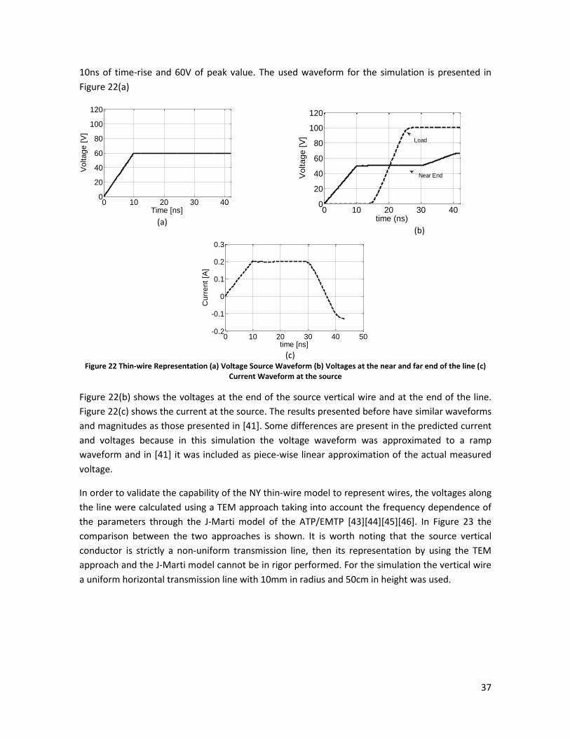
37
10ns of time-rise and 60V of peak value. The used waveform for the simulation is presented in
Figure 22(a)
(a)
(b)
(c)
Figure 22 Thin-wire Representation (a) Voltage Source Waveform (b) Voltages at the near and far end of the line (c) Current Waveform at the source
Figure 22(b) shows the voltages at the end of the source vertical wire and at the end of the line.
Figure 22(c) shows the current at the source. The results presented before have similar waveforms
and magnitudes as those presented in [41]. Some differences are present in the predicted current
and voltages because in this simulation the voltage waveform was approximated to a ramp
waveform and in [41] it was included as piece-wise linear approximation of the actual measured
voltage.
In order to validate the capability of the NY thin-wire model to represent wires, the voltages along
the line were calculated using a TEM approach taking into account the frequency dependence of
the parameters through the J-Marti model of the ATP/EMTP [43][44][45][46]. In Figure 23 the
comparison between the two approaches is shown. It is worth noting that the source vertical
conductor is strictly a non-uniform transmission line, then its representation by using the TEM
approach and the J-Marti model cannot be in rigor performed. For the simulation the vertical wire
a uniform horizontal transmission line with 10mm in radius and 50cm in height was used.
0 10 20 30 400
20
40
60
80
100
120
Time [ns]
Vo
lta
ge
[V
]
0 10 20 30 400
20
40
60
80
100
120
time (ns)
Vo
lta
ge
[V
]
Near End
Load
0 10 20 30 40 50-0.2
-0.1
0
0.1
0.2
0.3
Curr
ent
[A]
time [ns]
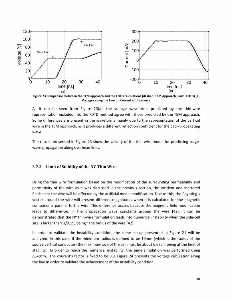
38
(a)
(b)
Figure 23 Comparison between the TEM approach and the FDTD calculations (dashed: TEM Approach, Solid: FDTD) (a) Voltages along the Line (b) Current at the source
As it can be seen from Figure 23(a), the voltage waveforms predicted by the thin-wire
representation included into the FDTD method agree with those predicted by the TEM approach.
Some differences are present in the waveforms mainly due to the representation of the vertical
wire in the TEM approach, as it produces a different reflection coefficient for the back-propagating
wave.
The results presented in Figure 23 show the validity of the thin-wire model for predicting surge-
wave propagation along overhead lines.
3.7.3 Limit of Stability of the NY-Thin Wire
Using the thin wire formulation based on the modification of the surrounding permeability and
permittivity of the wire as it was discussed in the previous section, the incident and scattered
fields near the wire will be affected by the artificial media modification. Due to this, the Poynting´s
vector around the wire will present different magnitudes when it is calculated for the magnetic
components parallel to the wire. This difference occurs because the magnetic field modification
leads to differences in the propagation wave constants around the wire [42]. It can be
demonstrated that the NY thin-wire formulation leads into numerical instability when the side-cell
size is larger than: r/0.15; being r the radius of the wire [42].
In order to validate the instability condition, the same set-up presented in Figure 21 will be
analyzed. In this case, if the minimum radius is defined to be 10mm (which is the radius of the
source vertical conductor) the maximum size of the cell must be about 6.67cm being at the limit of
stability. In order to reach the numerical instability, the same simulation was performed using
ΔS=8cm. The courant’s factor is fixed to be 0.9. Figure 24 presents the voltage calculation along
the line in order to validate the achievement of the instability condition.
0 10 20 30 400
20
40
60
80
100
120
Vo
lta
ge
[V
]
time [ns]
Far End
Near End
0 10 20 30 40-200
-100
0
100
200
300
Cu
rre
nt
[mA
]
time [ns]

39
Figure 24 Instability condition for radius lower than 0.15 times the cell-side size
As can be seen from Figure 24 the voltages along the line are well reproduced for the first time
instants. However, due to the error propagation caused by the Poynting’s vector difference
discussed before, the FDTD simulation becomes unstable at about 38ns.
3.7.4 Improved Noda-Yokoyama Model (INY)
The thin wire improvement proposed in [42], which will be referred as INY, proposes modifying
not only the magnetic relative permeability around the wire but also the components in the
vicinity in order to obtain the same Poyinting´s vector. The improved thin wire formulation was
included in the simulation using ΔS=8cm and maintaining the geometry as was proposed in Figure
21. The instability problem presented in Figure 24 was solved as it is shown in Figure 25.
0 10 20 30 400
20
40
60
80
100
120
time (ns)
Voltage [
V]
Instability due to the radius cell size relation
in the thin wire formulation
2m 3m1m0m
4m
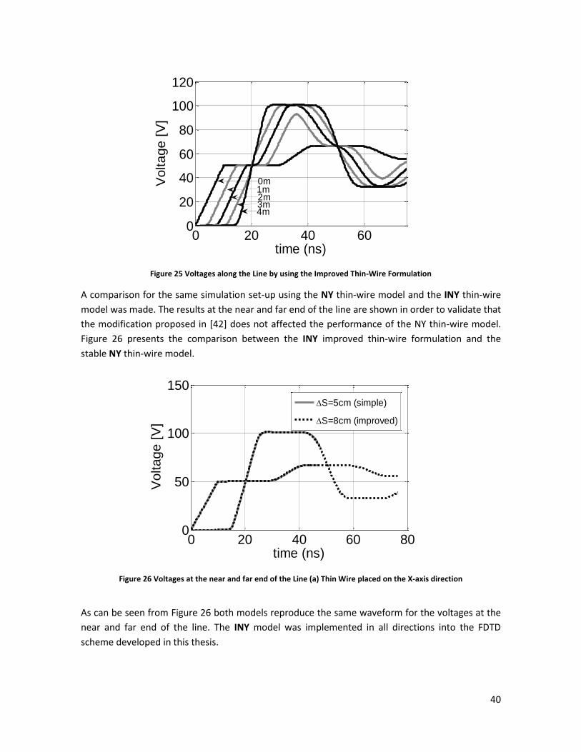
40
Figure 25 Voltages along the Line by using the Improved Thin-Wire Formulation
A comparison for the same simulation set-up using the NY thin-wire model and the INY thin-wire
model was made. The results at the near and far end of the line are shown in order to validate that
the modification proposed in [42] does not affected the performance of the NY thin-wire model.
Figure 26 presents the comparison between the INY improved thin-wire formulation and the
stable NY thin-wire model.
Figure 26 Voltages at the near and far end of the Line (a) Thin Wire placed on the X-axis direction
As can be seen from Figure 26 both models reproduce the same waveform for the voltages at the
near and far end of the line. The INY model was implemented in all directions into the FDTD
scheme developed in this thesis.
0 20 40 600
20
40
60
80
100
120
time (ns)
Vo
lta
ge
[V
]
4m3m2m1m0m
0 20 40 60 800
50
100
150
time (ns)
Vo
lta
ge
[V
]
S=5cm (simple)
S=8cm (improved)
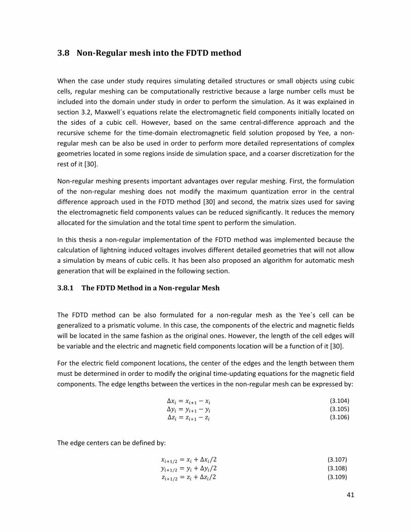
41
3.8 Non-Regular mesh into the FDTD method
When the case under study requires simulating detailed structures or small objects using cubic
cells, regular meshing can be computationally restrictive because a large number cells must be
included into the domain under study in order to perform the simulation. As it was explained in
section 3.2, Maxwell´s equations relate the electromagnetic field components initially located on
the sides of a cubic cell. However, based on the same central-difference approach and the
recursive scheme for the time-domain electromagnetic field solution proposed by Yee, a non-
regular mesh can be also be used in order to perform more detailed representations of complex
geometries located in some regions inside de simulation space, and a coarser discretization for the
rest of it [30].
Non-regular meshing presents important advantages over regular meshing. First, the formulation
of the non-regular meshing does not modify the maximum quantization error in the central
difference approach used in the FDTD method [30] and second, the matrix sizes used for saving
the electromagnetic field components values can be reduced significantly. It reduces the memory
allocated for the simulation and the total time spent to perform the simulation.
In this thesis a non-regular implementation of the FDTD method was implemented because the
calculation of lightning induced voltages involves different detailed geometries that will not allow
a simulation by means of cubic cells. It has been also proposed an algorithm for automatic mesh
generation that will be explained in the following section.
3.8.1 The FDTD Method in a Non-regular Mesh
The FDTD method can be also formulated for a non-regular mesh as the Yee´s cell can be
generalized to a prismatic volume. In this case, the components of the electric and magnetic fields
will be located in the same fashion as the original ones. However, the length of the cell edges will
be variable and the electric and magnetic field components location will be a function of it [30].
For the electric field component locations, the center of the edges and the length between them
must be determined in order to modify the original time-updating equations for the magnetic field
components. The edge lengths between the vertices in the non-regular mesh can be expressed by:
(3.104) (3.105) (3.106)
The edge centers can be defined by:
(3.107)
(3.108)
(3.109)
42
For the magnetic field location and its time-updating equation based on the electric field
component location, the lengths between the edge centers must be also determined. They will be
denoted by the letter h as:
(
*
(3.110)
(
*
(3.111)
(
*
(3.112)
Where and are the lengths of the cell sides at the ( ) location. Figure 27 shows
the location of the electric and magnetic field components, and the cell lengths definition taking
into account all of the expression presented before and using the same indexes notation as in
section 3.2.
(i, j, k)
ΔXi
Ex(i,j,k)
Hx(i,j,k)
x
yz
Ez(i,j+1,k)
Hz(i,j,k)
Δy(j)
ΔZk
Ey(i,j,k)
Ez(i,j,k)
Ex(i,j+1,k)
Hx(i+1,j,k)Hz(i+1,j,k)
Δhx(i)
Ey(i+1,j,k)
Hz(i,j,k+1)Hx(i+1,j,k)
Δhz(k)Ey(i,j,k+1)
Ex(i,j,k+1)
ΔXi+1
ΔZk+1
Figure 27 Location of the electric and magnetic field component in the non-regular cell
As it can be seen from Figure 27, the electric and magnetic field components are calculated at
convenient locations in order to apply the finite difference formulation for the Maxwell’s
equations. This figure shows three Yee’s cells adjacent to each other where different side lengths
are considered for the cell located at the (i,j,k) node. It must be also note that due to the different
cell-side lengths for each direction , and , , the distances and between
the components will also change for each direction.
Finally, the electric field and magnetic field components can be found by similar time-updating
equations presented in previous sections but taking into account the non-regular location of the
edge centers, the variable cell-length and the distances between each edge center.
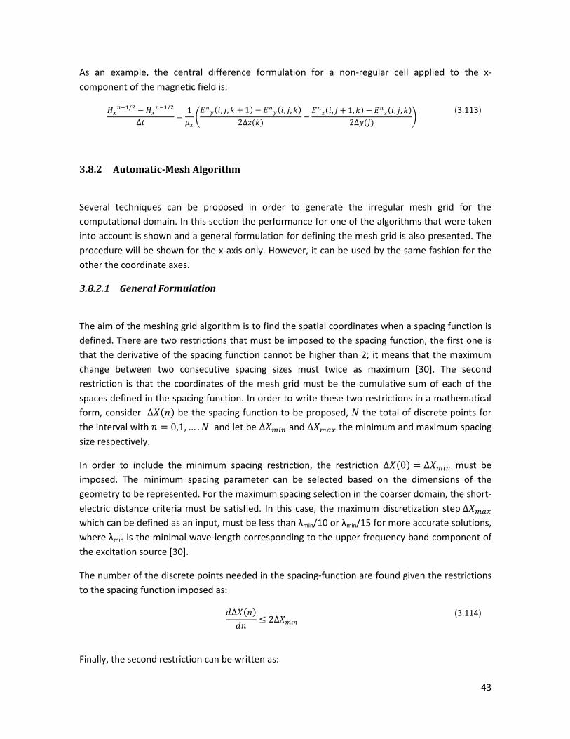
43
As an example, the central difference formulation for a non-regular cell applied to the x-
component of the magnetic field is:
(
( ) ( )
( )
( )
( )
( ))
(3.113)
3.8.2 Automatic-Mesh Algorithm
Several techniques can be proposed in order to generate the irregular mesh grid for the
computational domain. In this section the performance for one of the algorithms that were taken
into account is shown and a general formulation for defining the mesh grid is also presented. The
procedure will be shown for the x-axis only. However, it can be used by the same fashion for the
other the coordinate axes.
3.8.2.1 General Formulation
The aim of the meshing grid algorithm is to find the spatial coordinates when a spacing function is
defined. There are two restrictions that must be imposed to the spacing function, the first one is
that the derivative of the spacing function cannot be higher than 2; it means that the maximum
change between two consecutive spacing sizes must twice as maximum [30]. The second
restriction is that the coordinates of the mesh grid must be the cumulative sum of each of the
spaces defined in the spacing function. In order to write these two restrictions in a mathematical
form, consider ( ) be the spacing function to be proposed, the total of discrete points for
the interval with and let be and the minimum and maximum spacing
size respectively.
In order to include the minimum spacing restriction, the restriction ( ) must be
imposed. The minimum spacing parameter can be selected based on the dimensions of the
geometry to be represented. For the maximum spacing selection in the coarser domain, the short-
electric distance criteria must be satisfied. In this case, the maximum discretization step
which can be defined as an input, must be less than λmin/10 or λmin/15 for more accurate solutions,
where λmin is the minimal wave-length corresponding to the upper frequency band component of
the excitation source [30].
The number of the discrete points needed in the spacing-function are found given the restrictions
to the spacing function imposed as:
( )
(3.114)
Finally, the second restriction can be written as:
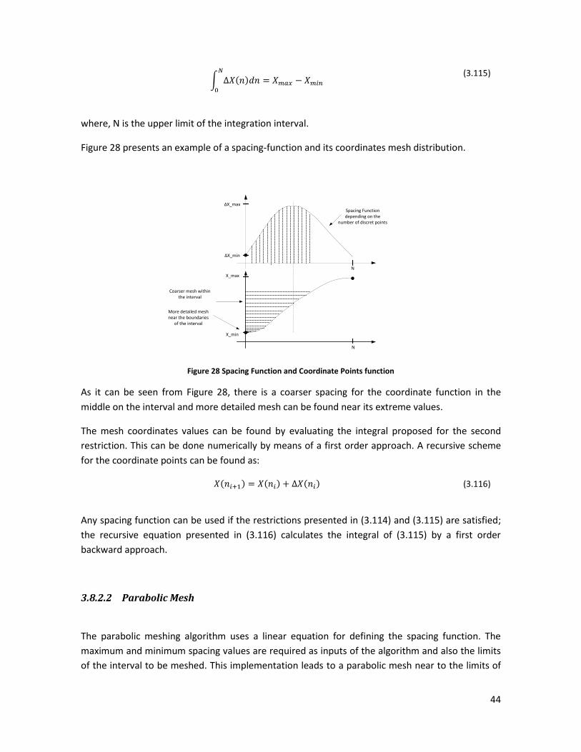
44
∫ ( )
(3.115)
where, N is the upper limit of the integration interval.
Figure 28 presents an example of a spacing-function and its coordinates mesh distribution.
∆X_min
∆X_max
N
X_min
X_max
N
Spacing Function depending on the
number of discret points
More detailed mesh near the boundaries
of the interval
Coarser mesh within the interval
Figure 28 Spacing Function and Coordinate Points function
As it can be seen from Figure 28, there is a coarser spacing for the coordinate function in the
middle on the interval and more detailed mesh can be found near its extreme values.
The mesh coordinates values can be found by evaluating the integral proposed for the second
restriction. This can be done numerically by means of a first order approach. A recursive scheme
for the coordinate points can be found as:
( ) ( ) ( ) (3.116)
Any spacing function can be used if the restrictions presented in (3.114) and (3.115) are satisfied;
the recursive equation presented in (3.116) calculates the integral of (3.115) by a first order
backward approach.
3.8.2.2 Parabolic Mesh
The parabolic meshing algorithm uses a linear equation for defining the spacing function. The
maximum and minimum spacing values are required as inputs of the algorithm and also the limits
of the interval to be meshed. This implementation leads to a parabolic mesh near to the limits of

45
the algorithm and a linear meshing within the interval; Figure 29 depicts the parabolic meshing
algorithm.
∆X_min
∆X_max
N
X_min
X_max
N
Parabolic Increasing
Parabolic decreasing
Number of Discrete Points
Number of Discrete Points
Spacing Function
Parabolic detailed mesh near the
boundaries of the interval
Coarser mesh within the interval
n1 n2 n1
Figure 29 Parabolic Mesh based on a trapezoidal spacing function
The spacing function can be written as a piecewise function defined by:
( )
( )
(3.117)
Where is the slope of the straight line and .
In order to obtain n1, the restriction on the maximum spacing function derivative must be
imposed. As the spacing function has the same linear variation on the increasing and decreasing
sections, the derivative of the function can be evaluated in the first interval as:
( )
(3.118)
(3.119) ( ) (3.120)
The slope can be calculated from the desired spacing rate. In general where
can be set between in order to consider the minimum and maximum slope
respectively. The factor can be understood as a decreasing or increasing factor for the spacing
rate; factors lower than 1 implies soft changes on the spacing mesh.
Using the definition of the second restriction for the spacing function we will have:

46
∫ ( )
(3.121)
Using this restriction it is obtained that:
( )
(3.122)
Where n2 can be found by means of the expression:
( ) ( )
(3.123)
The spacing function has now been completely defined and the integration over the interval is
performed numerically. Figure 30 show the automatic parabolic-mesh for an interval [100mm,
975mm] using a minimum spacing of 2.5mm and a maximum of 55mm. As can be seen from the
Figure 30(b), 26 discrete points are needed for the entire interval using the irregular mesh instead
of 350.000 discrete points required using the traditional regular meshing.
(a)
(b)
Figure 30 Parabolic Mesh Algorithm (a) Example of a Spacing Function (b) Coordinate mesh nodes
0 5 10 15 20 25 300
20
40
60
(n
) [m
m]
n
0 5 10 15 20 25 300
0.5
1
X[m
]
n0.2 0.4 0.6 0.8 1
0
0.2
0.4
0.6
0.8
1
X [m]
Y [m
]
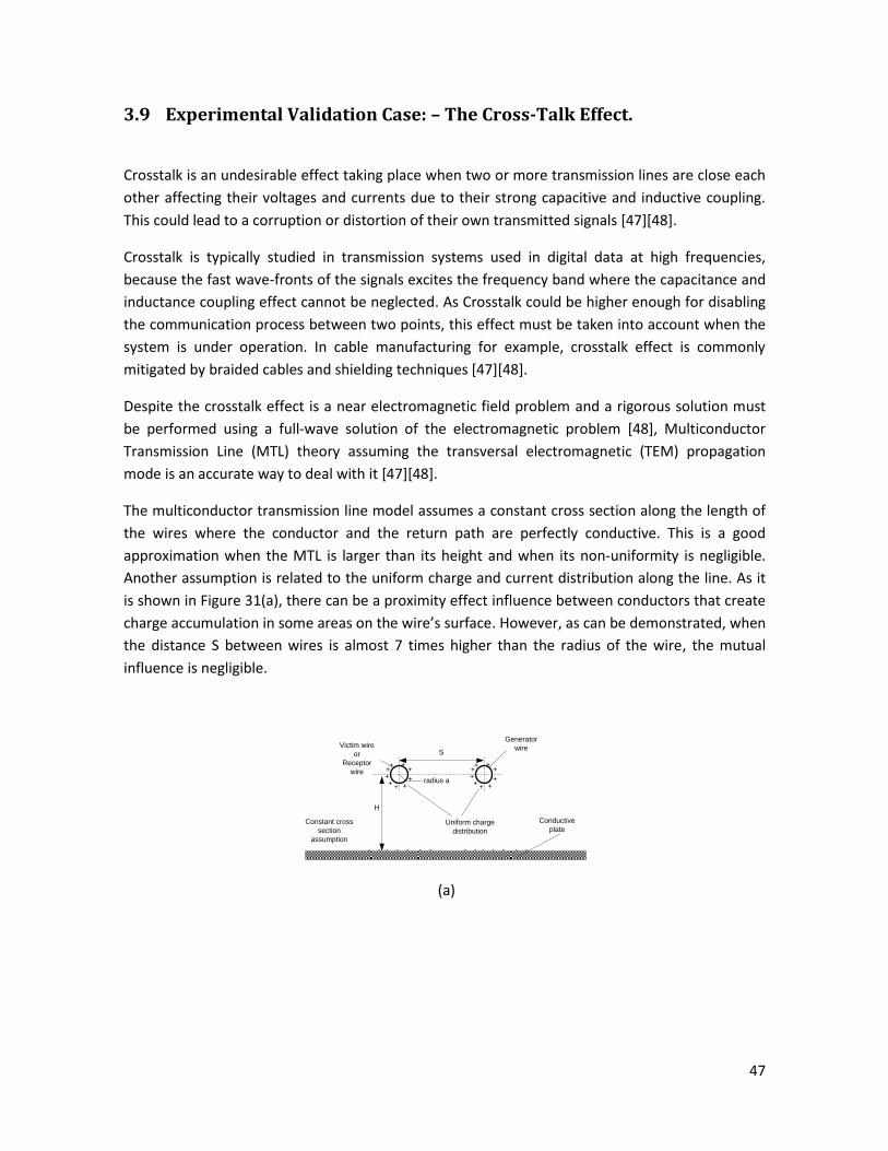
47
3.9 Experimental Validation Case: – The Cross-Talk Effect.
Crosstalk is an undesirable effect taking place when two or more transmission lines are close each
other affecting their voltages and currents due to their strong capacitive and inductive coupling.
This could lead to a corruption or distortion of their own transmitted signals [47][48].
Crosstalk is typically studied in transmission systems used in digital data at high frequencies,
because the fast wave-fronts of the signals excites the frequency band where the capacitance and
inductance coupling effect cannot be neglected. As Crosstalk could be higher enough for disabling
the communication process between two points, this effect must be taken into account when the
system is under operation. In cable manufacturing for example, crosstalk effect is commonly
mitigated by braided cables and shielding techniques [47][48].
Despite the crosstalk effect is a near electromagnetic field problem and a rigorous solution must
be performed using a full-wave solution of the electromagnetic problem [48], Multiconductor
Transmission Line (MTL) theory assuming the transversal electromagnetic (TEM) propagation
mode is an accurate way to deal with it [47][48].
The multiconductor transmission line model assumes a constant cross section along the length of
the wires where the conductor and the return path are perfectly conductive. This is a good
approximation when the MTL is larger than its height and when its non-uniformity is negligible.
Another assumption is related to the uniform charge and current distribution along the line. As it
is shown in Figure 31(a), there can be a proximity effect influence between conductors that create
charge accumulation in some areas on the wire’s surface. However, as can be demonstrated, when
the distance S between wires is almost 7 times higher than the radius of the wire, the mutual
influence is negligible.
S
H
Conductive
plate
radius a
Constant cross
section
assumption
Generator
wireVictim wire
or
Receptor
wire
++++ +
+
+++
++++ +
+
+++
Uniform charge
distribution
- -- - - - - - -- - - - -
(a)

48
Generator wire
Victim wireL
Source
RsRne
Load
Rfe
I
Far endNear end
Self
Inductance
Mutual
Inductance
(b)
Figure 31(a) Schematic Representation of capacitive coupling for two wires above a conductive return plate (cross section). (b) Schematic Representation of inductive coupling for two wires above a conductive return plate (lateral
section)
Current along the wire is assumed to be constant along an infinitesimal length allowing writing
magnetic field expressions only from the geometric constants associated to the line conductors as
it shown Figure 31(b). Finally, the consideration about a perfect conducting wire, can be easily
overcome by the cuasi-TEM approximation where the electric field in the direction of propagation
is neglected for low resistance values.
These assumptions allow having a transversal electromagnetic field along the line and voltages
and current relation can be easily derived from this EM field formulation [47][48]. The well-known
formulation for currents and voltages in the generator and receptor wire is presented as follows
( )
( )
( )
(3.124)
( )
( )
( )
(3.125)
( )
( )
( )
( )
(3.126)
( )
( )
( )
( )
(3.127)
Where , and are the self-inductance and mutual inductance and CG, CR and Cm are the self-
capacitance and mutual capacitance for the generator and receptor wire respectively.
An experimental set up was implemented in order to compare the theoretically obtained results
by computation and measured data. The set up was composed by two copper wires with a DC
resistance per unit length of 84Ω/km located next to each other with a distance of 1.5cm between
them. The radius of the wire was about 0.25mm. Each wire was horizontally at the same height of
5.5cm from a conductive plate. The resistivity of the plate was assumed to be 1.69x10⁻⁸Ωm. The
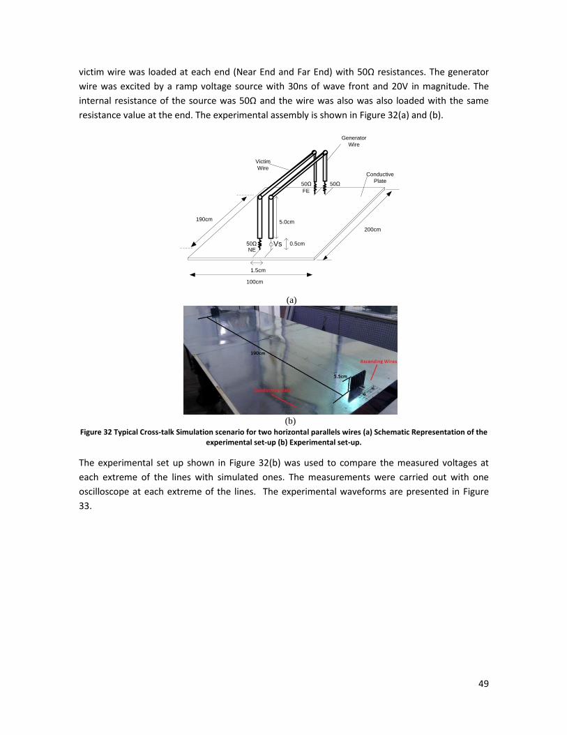
49
victim wire was loaded at each end (Near End and Far End) with 50Ω resistances. The generator
wire was excited by a ramp voltage source with 30ns of wave front and 20V in magnitude. The
internal resistance of the source was 50Ω and the wire was also was also loaded with the same
resistance value at the end. The experimental assembly is shown in Figure 32(a) and (b).
200cm
1.5cm
190cm5.0cm
0.5cmVs
50Ω50Ω
50Ω
100cm
Conductive
Plate
Generator
Wire
Victim
Wire
NE
FE
(a)
(b)
Figure 32 Typical Cross-talk Simulation scenario for two horizontal parallels wires (a) Schematic Representation of the experimental set-up (b) Experimental set-up.
The experimental set up shown in Figure 32(b) was used to compare the measured voltages at
each extreme of the lines with simulated ones. The measurements were carried out with one
oscilloscope at each extreme of the lines. The experimental waveforms are presented in Figure
33.
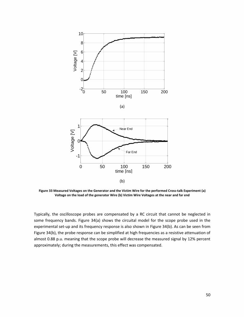
50
(a)
(b)
Figure 33 Measured Voltages on the Generator and the Victim Wire for the performed Cross-talk Experiment (a) Voltage on the load of the generator Wire (b) Victim Wire Voltages at the near and far end
Typically, the oscilloscope probes are compensated by a RC circuit that cannot be neglected in
some frequency bands. Figure 34(a) shows the circuital model for the scope probe used in the
experimental set-up and its frequency response is also shown in Figure 34(b). As can be seen from
Figure 34(b), the probe response can be simplified at high frequencies as a resistive attenuation of
almost 0.88 p.u. meaning that the scope probe will decrease the measured signal by 12% percent
approximately; during the measurements, this effect was compensated.
0 50 100 150 200-2
0
2
4
6
8
10
Voltage [
V]
time [ns]
0 50 100 150 200
-1
0
1
Vo
lta
ge
[V
]
time [ns]
Near End
Far End
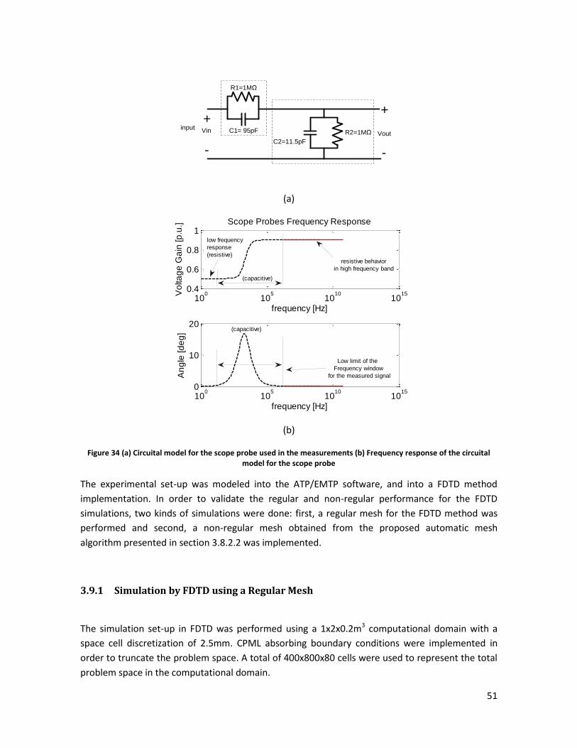
51
R1=1MΩ
R2=1MΩC1= 95pF
C2=11.5pF
VinVout
+
-
+
-
input
(a)
(b)
Figure 34 (a) Circuital model for the scope probe used in the measurements (b) Frequency response of the circuital model for the scope probe
The experimental set-up was modeled into the ATP/EMTP software, and into a FDTD method
implementation. In order to validate the regular and non-regular performance for the FDTD
simulations, two kinds of simulations were done: first, a regular mesh for the FDTD method was
performed and second, a non-regular mesh obtained from the proposed automatic mesh
algorithm presented in section 3.8.2.2 was implemented.
3.9.1 Simulation by FDTD using a Regular Mesh
The simulation set-up in FDTD was performed using a 1x2x0.2m3 computational domain with a
space cell discretization of 2.5mm. CPML absorbing boundary conditions were implemented in
order to truncate the problem space. A total of 400x800x80 cells were used to represent the total
problem space in the computational domain.
100
105
1010
1015
0.4
0.6
0.8
1Scope Probes Frequency Response
Vo
lta
ge
Ga
in [p
.u.]
frequency [Hz]
100
105
1010
1015
0
10
20
An
gle
[d
eg
]
frequency [Hz]
low frequency
response
(resistive)
Low limit of the
Frequency window
for the measured signal
(capacitive)
(capacitive)
resistive behavior
in high frequency band
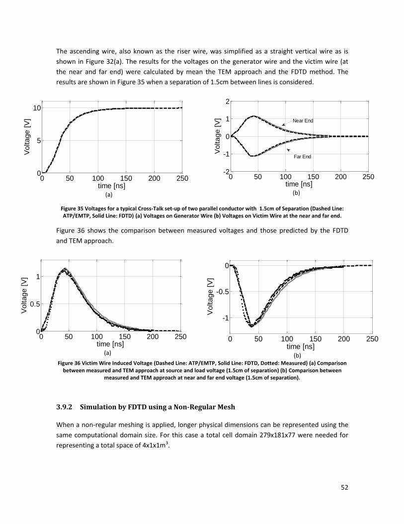
52
The ascending wire, also known as the riser wire, was simplified as a straight vertical wire as is
shown in Figure 32(a). The results for the voltages on the generator wire and the victim wire (at
the near and far end) were calculated by mean the TEM approach and the FDTD method. The
results are shown in Figure 35 when a separation of 1.5cm between lines is considered.
(a)
(b)
Figure 35 Voltages for a typical Cross-Talk set-up of two parallel conductor with 1.5cm of Separation (Dashed Line: ATP/EMTP, Solid Line: FDTD) (a) Voltages on Generator Wire (b) Voltages on Victim Wire at the near and far end.
Figure 36 shows the comparison between measured voltages and those predicted by the FDTD
and TEM approach.
(a)
(b)
Figure 36 Victim Wire Induced Voltage (Dashed Line: ATP/EMTP, Solid Line: FDTD, Dotted: Measured) (a) Comparison between measured and TEM approach at source and load voltage (1.5cm of separation) (b) Comparison between
measured and TEM approach at near and far end voltage (1.5cm of separation).
3.9.2 Simulation by FDTD using a Non-Regular Mesh
When a non-regular meshing is applied, longer physical dimensions can be represented using the
same computational domain size. For this case a total cell domain 279x181x77 were needed for
representing a total space of 4x1x1m3.
0 50 100 150 200 2500
5
10
time [ns]
Voltage [
V]
0 50 100 150 200 250-2
-1
0
1
2
time [ns]
Vo
lta
ge
[V
]
Near End
Far End
0 50 100 150 200 2500
0.5
1
time [ns]
Vo
lta
ge
[V
]
0 50 100 150 200 250
-1
-0.5
0
time [ns]
Vo
lta
ge
[V
]
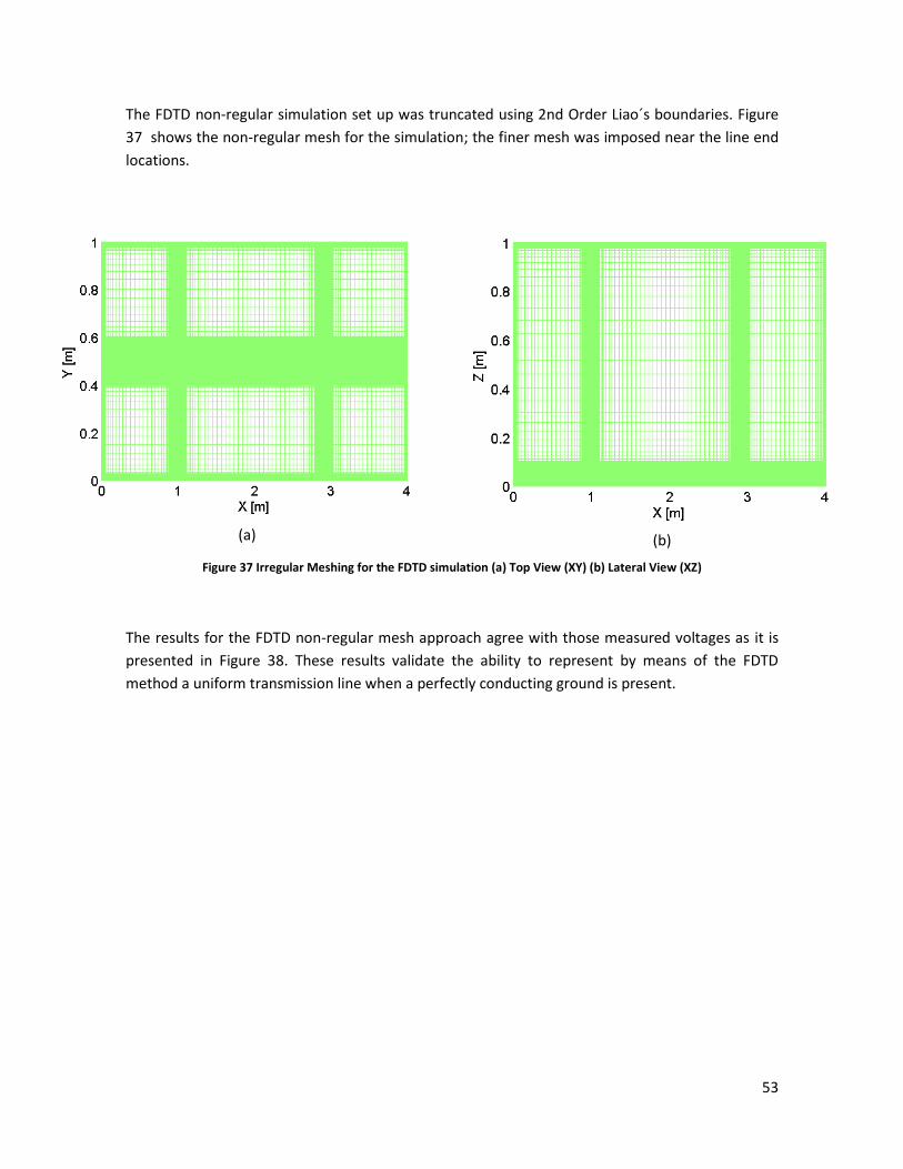
53
The FDTD non-regular simulation set up was truncated using 2nd Order Liao´s boundaries. Figure
37 shows the non-regular mesh for the simulation; the finer mesh was imposed near the line end
locations.
(a)
(b)
Figure 37 Irregular Meshing for the FDTD simulation (a) Top View (XY) (b) Lateral View (XZ)
The results for the FDTD non-regular mesh approach agree with those measured voltages as it is
presented in Figure 38. These results validate the ability to represent by means of the FDTD
method a uniform transmission line when a perfectly conducting ground is present.

54
(a)
(b)
Figure 38 Voltages on the Victim Wire (dotted: Measured, solid: FDTD non-regular mesh) (a) Voltage at the Near End (b) Voltage at the Far End
0 50 100 150 200 2500
0.5
1
1.5
Voltage [
V]
time [ns]
0 50 100 150 200 250-1.5
-1
-0.5
0
Voltage [
V]
time [ns]

55
4 Radiated Electromagnetic Field
Electromagnetic radiation occurs when a time-varying source is present in a region of the space,
allowing the interaction of electric and magnetic fields in the medium and its propagation through
the space [49]. Most of the analysis made on electromagnetic radiation are based on the Hertzian
dipole concept in which a pair of wires of a finite length are excited at the middle by a voltage
source as it is shown in Figure 39(a).
V(t) l
I
I
y
x
z
(a)
lImax
(b)
Imax l
(c)
Figure 39 (a) Dipole Antenna (b) Current Distribution for a half-wave dipole (c) Current-Element Dipole
In order to calculate the radiation of the dipole, the distribution current along it must be known.
This current distribution can be found by means of the scattered field formulation and the solution
of the resulting integral equation. This integral equation can be solved by several numerical
techniques being the Method of Moments (MoM) one of the most popular approaches for solving
the current distribution along conducting wires in the frequency domain [49]. When the length of
the wires is finite, the current distribution of the Hertizian dipole is maxima at the middle and
decreases to the ends as is shown in Figure 39(b). The simplest representation of a radiating dipole
is that known as the infinitesimal dipole or current dipole [16][49], where its current distribution
along the segment is assumed to be constant even if it is finite in length as is shown in Figure
39(c).
This assumption simplifies enormously the calculation of radiated fields due to vertical current
dipoles and it will be fundamental for the calculation of lightning electromagnetic fields as will be
shown in chapter 5.
4.1 Radiating Vertical-Current Dipole over a homogeneous ground.
The geometry when a Cartesian coordinate system is assumed is shown in Figure 40.

56
I
Y
X
Z
R0Ez
Er
θd
R
H
dl
Figure 40 Vertical electric current dipole radiation in the free-Space
As the vertical dipole is defined to have z-directed current, the magnetic vector potential will have
only z-axis component and will be given by:
(4.1)
The term will be omitted during the following. Once the magnetic vector potential is
obtained, the magnetic field components can be also found [16] by using:
(4.2)
The electric radiated fields due to a vertical current element in the free space can be calculated by
the Maxwell equations. Selecting a cylindrical coordinates system as the most convenient for the
vertical current dipole representation, the magnetic and electric field components can be
calculated from:
(
* (4.3)
(
( ) *
(4.4)
( ( ) [
( ) ]*
(4.5)
Expressions (4.3), (4.4) and (4.5) allow calculating the radiated electromagnetic fields in free space
due to a vertical current dipole.
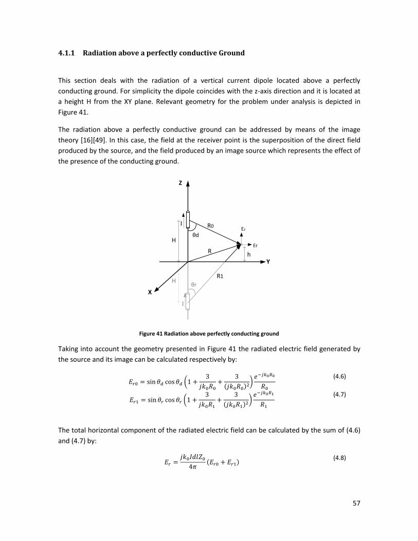
57
4.1.1 Radiation above a perfectly conductive Ground
This section deals with the radiation of a vertical current dipole located above a perfectly
conducting ground. For simplicity the dipole coincides with the z-axis direction and it is located at
a height H from the XY plane. Relevant geometry for the problem under analysis is depicted in
Figure 41.
The radiation above a perfectly conductive ground can be addressed by means of the image
theory [16][49]. In this case, the field at the receiver point is the superposition of the direct field
produced by the source, and the field produced by an image source which represents the effect of
the presence of the conducting ground.
I
Y
X
Z
R0Ez
Er
θd
R
H
H
I
R1
θr
h
Figure 41 Radiation above perfectly conducting ground
Taking into account the geometry presented in Figure 41 the radiated electric field generated by
the source and its image can be calculated respectively by:
(
( ) *
(4.6)
(
( ) *
(4.7)
The total horizontal component of the radiated electric field can be calculated by the sum of (4.6)
and (4.7) by:
( )
(4.8)

58
The same for the vertical radiated electric field component,
( ( ) [
( ) ]*
(4.9)
( ( ) [
( ) ]*
(4.10)
Finally, the total vertical component can be calculated adding (4.9) and (4.10):
( )
(4.11)
Next sections will consider a finite conductively ground where the image theory cannot be used as
presented in this section.
4.1.2 Radiation above a Flat Homogeneous ground
In this section a finite conducting ground is taken into account for the radiated field calculations.
The assumption of perfectly conducting ground is unpractical when poorly conductive grounds are
present. Figure 42 depicts the scenario and the relevant geometry for this case.
θr-z
Y
X
Z
z
R0
h
R1
Ez
Er
h
d
Idl
Flat Homogeneous Ground
σ1, μ1, ε1
Airσ0, μ0, ε0
Image dipole
θd
Figure 42 Vertical Current Dipole above Homogeneous Finitely Conducting Ground
Radiation above homogeneous ground represents a difficulty in evaluating the effect of the
ground presence. This problem was addressed initially by Sommerfeld, who proposed a solution in
order to calculate the radiated electric field for a current dipole [16].
4.1.2.1 Sommerfeld’s Solution
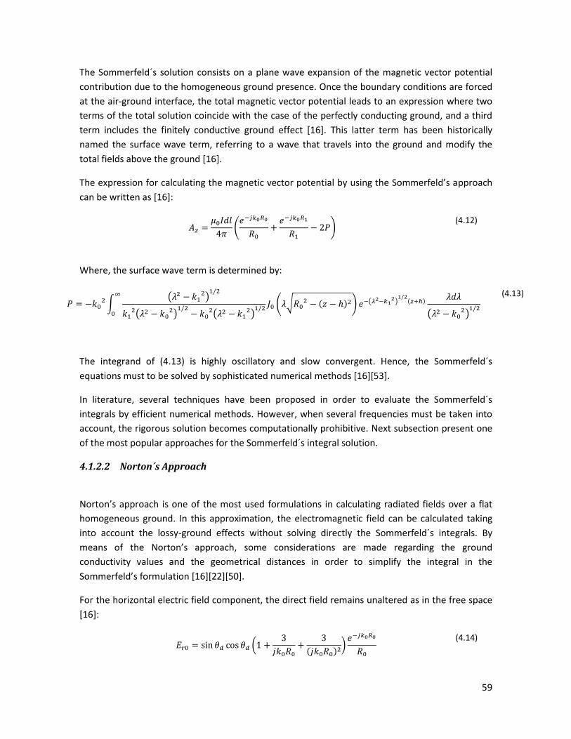
59
The Sommerfeld´s solution consists on a plane wave expansion of the magnetic vector potential
contribution due to the homogeneous ground presence. Once the boundary conditions are forced
at the air-ground interface, the total magnetic vector potential leads to an expression where two
terms of the total solution coincide with the case of the perfectly conducting ground, and a third
term includes the finitely conductive ground effect [16]. This latter term has been historically
named the surface wave term, referring to a wave that travels into the ground and modify the
total fields above the ground [16].
The expression for calculating the magnetic vector potential by using the Sommerfeld’s approach
can be written as [16]:
(
) (4.12)
Where, the surface wave term is determined by:
∫
( )
(
)
(
)
( √ ( ) )
( )
( )
( )
(4.13)
The integrand of (4.13) is highly oscillatory and slow convergent. Hence, the Sommerfeld´s
equations must to be solved by sophisticated numerical methods [16][53].
In literature, several techniques have been proposed in order to evaluate the Sommerfeld´s
integrals by efficient numerical methods. However, when several frequencies must be taken into
account, the rigorous solution becomes computationally prohibitive. Next subsection present one
of the most popular approaches for the Sommerfeld´s integral solution.
4.1.2.2 Norton´s Approach
Norton’s approach is one of the most used formulations in calculating radiated fields over a flat
homogeneous ground. In this approximation, the electromagnetic field can be calculated taking
into account the lossy-ground effects without solving directly the Sommerfeld´s integrals. By
means of the Norton’s approach, some considerations are made regarding the ground
conductivity values and the geometrical distances in order to simplify the integral in the
Sommerfeld’s formulation [16][22][50].
For the horizontal electric field component, the direct field remains unaltered as in the free space
[16]:
(
( ) *
(4.14)

60
The contribution on the horizontal electric field due to the ground presence can be written as [16]:
( ( )
( ) *
( ) [ ( )
]
(4.15)
Finally, the total horizontal field can be calculated by:
( )
(4.16)
For the vertical electric field, the direct contribution can be also calculated as in free-space by:
( ( ) [
( ) ]*
(4.17)
The contribution on the vertical electric field due to the ground presence can be written as [16]:
( ( ) ( ) (
*
( ) [
( ) ]*
(4.18)
Finally, the total vertical field component can be calculated by:
( )
(4.19)
In expression (4.15) and (4.18), represents the reflection coefficient and can be calculated by:
(4.20)
where,
√ (4.21)
and
(4.22)

61
√ ( ) is the propagation constant for the lossy ground and √ is
the propagation constant for air. The function is also called the normalized surface impedance.
The ( ) function also present in (4.15) and (4.18), is known as the attenuation function and can
be calculated by:
( ) √ ( √ ) (4.23)
The function is expressed by:
( )
(4.24)
The attenuation function proposed by Norton has been compared with the rigorous solution from
the Sommerfeld integrals and it has shown a good agreement for almost all far-field situations and
for the near field when considerably good ground conductivity is assumed. It must be taken into
account for calculations using the Norton´s approach, that the proposed results have used the
approximation that
.
In Figure 43(a) there is a comparison of the attenuation function magnitude between the
Sommerfeld’s solution and the Norton´s approach when a vertical dipole is radiating at 1MHz over
a flat ground, and with ρ=100Ωm and ε=10ε0 in resistivity and permittivity respectively.
Figure 43 Attenuation Function Magnitude Comparison for a Vertical Current-Dipole above a Flat Homogeneous Ground. Norton Approach (dashed lines) and Sommerfeld’s solution (circles) taken from [52]
0 5 10 1510
-2
10-1
100
101
X [km]
Att
en
ua
tio
n F
un
ctio
n |F w
|
Sommerfeld
Norton1 MHz
5MHz
10MHz
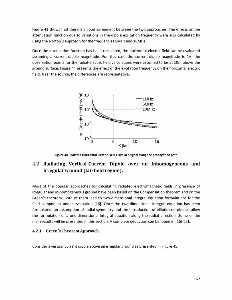
62
Figure 43 shows that there is a good agreement between the two approaches. The effects on the
attenuation function due to variations in the dipole excitation frequency were also calculated by
using the Norton´s approach for the frequencies 5MHz and 10MHz.
Once the attenuation function has been calculated, the horizontal electric field can be evaluated
assuming a current-dipole magnitude. For this case the current-dipole magnitude is 1A; the
observation points for the radial-electric field calculations were assumed to be at 10m above the
ground surface. Figure 44 presents the effect of the excitation frequency on the horizontal electric
field. Near the source, the differences are representative.
Figure 44 Radiated Horizontal Electric Field (10m in height) along the propagation path
4.2 Radiating Vertical-Current Dipole over an Inhomogeneous and
Irregular Ground (far-field region).
Most of the popular approaches for calculating radiated electromagnetic fields in presence of
irregular and in-homogeneous ground have been based on the Compensation theorem and on the
Green´s theorem. Both of them lead to two-dimensional integral equation formulations for the
field component under evaluation [16]. Once the two-dimensional integral equation has been
formulated, an assumption of radial symmetry and the introduction of elliptic coordinates allow
the formulation of a one-dimensional integral equation along the radial direction. Some of the
main results will be presented in this section. A complete deduction can be found in [16][53].
4.2.1 Green´s Theorem Approach
Consider a vertical current dipole above an irregular ground as presented in Figure 45.
0 5 10 1510
-4
10-2
100
102
X [km]
Hor.
Ele
ctr
ic F
ield
[m
V/m
]
1MHz
5MHz
10MHz
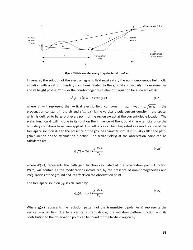
63
Vertical Current Dipole
Unperturbed Terrain Profile
Observation Point
P
Integration Point
R1
R2
R0
x
Terrain Profile
d
R
Figure 45 Relevant Geometry Irregular Terrain profile.
In general, the solution of the electromagnetic field must satisfy the non-homogenous Helmholtz
equation with a set of boundary conditions related to the ground conductivity inhomogeneities
and its height profile. Consider the non-homogenous Helmhotlz equation for a scalar field :
( ) (4.25)
where will represent the vertical electric field component, √ is the
propagation constant in the air and ( ) is the vertical dipole current density in the space,
which is defined to be zero at every point of the region except at the current-dipole location. The
scalar function will include in its solution the influence of the ground characteristics once the
boundary conditions have been applied. This influence can be interpreted as a modification of the
free-space solution due to the presence of the ground characteristics; It is usually called the path-
gain function or the attenuation function. The scalar field at the observation point can be
calculated as:
( ) ( )
(4.26)
where ( ), represents the path gain function calculated at the observation point. Function
( ) will contain all the modifications introduced by the presence of non-homogeneities and
irregularities of the ground and its effects on the observation point.
The free-space solution , is calculated by:
( ) ( )
(4.27)
Where ( ) represents the radiation pattern of the transmitter dipole. As represents the
vertical electric field due to a vertical current dipole, the radiation pattern function and its
contribution to the observation point can be found for the far-field region by:
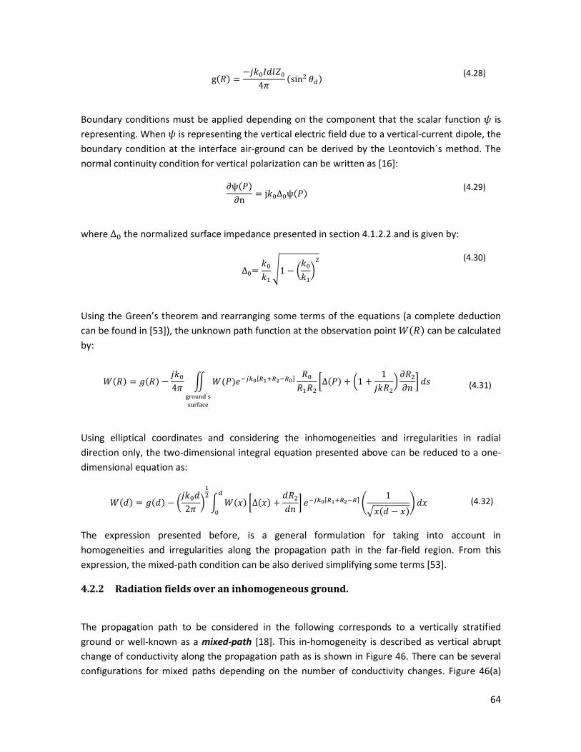
64
( )
( )
(4.28)
Boundary conditions must be applied depending on the component that the scalar function is
representing. When is representing the vertical electric field due to a vertical-current dipole, the
boundary condition at the interface air-ground can be derived by the Leontovich´s method. The
normal continuity condition for vertical polarization can be written as [16]:
( )
( )
(4.29)
where the normalized surface impedance presented in section 4.1.2.2 and is given by:
√ (
*
(4.30)
Using the Green’s theorem and rearranging some terms of the equations (a complete deduction
can be found in [53]), the unknown path function at the observation point ( ) can be calculated
by:
( ) ( )
∬ ( )
[ ( ) (
*
] (4.31)
Using elliptical coordinates and considering the inhomogeneities and irregularities in radial
direction only, the two-dimensional integral equation presented above can be reduced to a one-
dimensional equation as:
( ) ( ) (
*
∫ ( ) [ ( )
] (
√ ( ))
(4.32)
The expression presented before, is a general formulation for taking into account in
homogeneities and irregularities along the propagation path in the far-field region. From this
expression, the mixed-path condition can be also derived simplifying some terms [53].
4.2.2 Radiation fields over an inhomogeneous ground.
The propagation path to be considered in the following corresponds to a vertically stratified
ground or well-known as a mixed-path [18]. This in-homogeneity is described as vertical abrupt
change of conductivity along the propagation path as is shown in Figure 46. There can be several
configurations for mixed paths depending on the number of conductivity changes. Figure 46(a)

65
depicts the general geometry for a mixed-path of two-sections and Figure 46(b) for a mixed-path
of three-sections.
d
σ1, ε1, μ 1σ2, ε2, μ2
Vertical Current Dipole
dl
Observation Point
(a)
L1 L2
σ1, ε1, μ 1 σ3, ε3, μ3
Vertical Current Dipole
σ2, ε2, μ2
d
Observation Point
dL2
dL1
(b)
Figure 46 (a) Two-Sections Mixed-Path Condition (b) Three-Section Mixed-Path
One of the most popular analysis of the propagation effect due to the presence of a mixed path is
that proposed by Wait based on the compensation theorem approach [55][56][57][58], where the
attenuation function at the observation point can be expressed by:
( ) ( ) (
*
∫ ( ) ( )
√ ( )
(4.33)
The attenuation functions and are the attenuation functions for regions 1 and segment 2
respectively. The solution proposed by Wait assumes that both the vertical-current dipole and the
observation point are located at the ground surface and the observation point must be in the far
field region.
The attenuation functions and are obtained using the same idea as the attenuation
function proposed by Norton when a homogeneous ground is considered. Nevertheless, in this
case and will be dependent on the normalized impedance at each position in order to take
into account the longitudinal change of the ground conductivity. Some variables presented in the
attenuation function derived in the Norton’s approach have been redefined with the aim for
maintaining the same notation from Wait. The attenuation function can be written as:
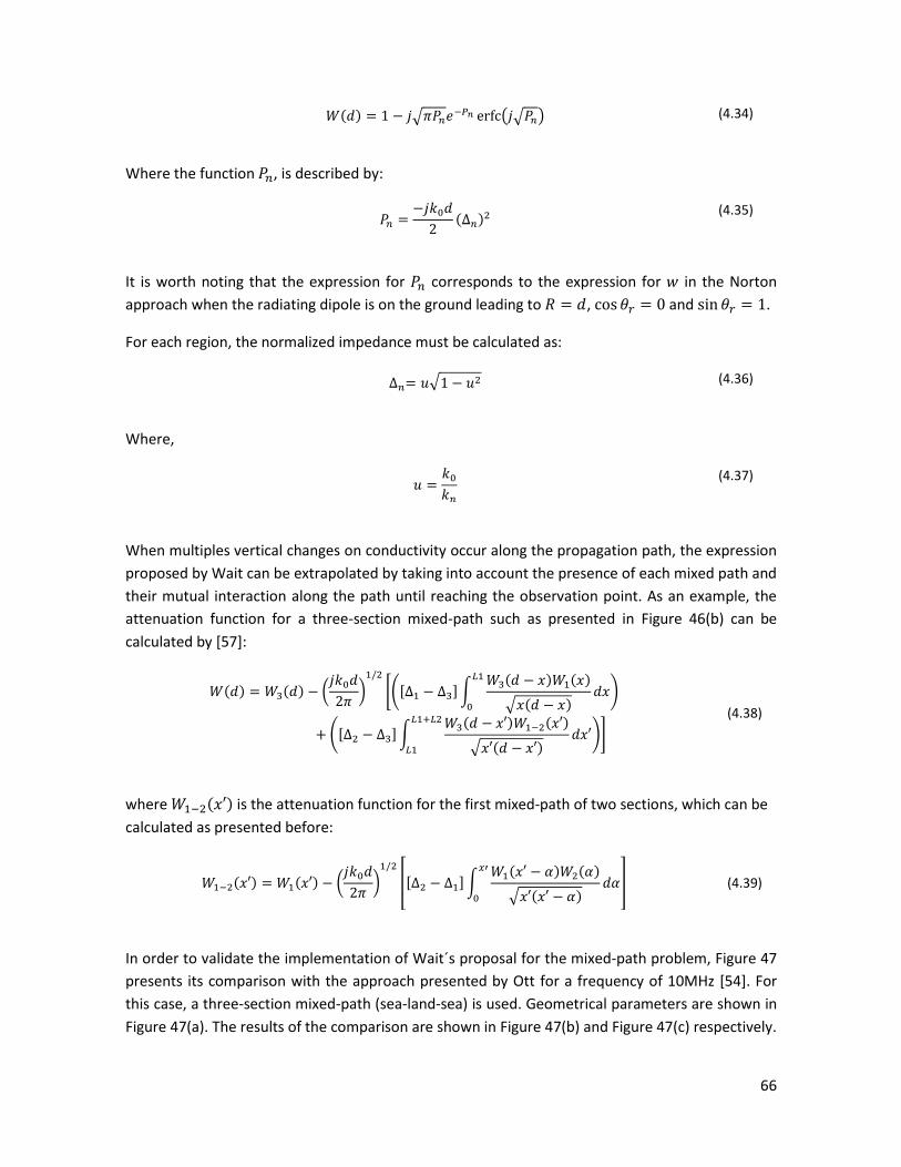
66
( ) √ ( √ ) (4.34)
Where the function , is described by:
( )
(4.35)
It is worth noting that the expression for corresponds to the expression for in the Norton
approach when the radiating dipole is on the ground leading to , and .
For each region, the normalized impedance must be calculated as:
√ (4.36)
Where,
(4.37)
When multiples vertical changes on conductivity occur along the propagation path, the expression
proposed by Wait can be extrapolated by taking into account the presence of each mixed path and
their mutual interaction along the path until reaching the observation point. As an example, the
attenuation function for a three-section mixed-path such as presented in Figure 46(b) can be
calculated by [57]:
( ) ( ) (
*
*( ∫ ( ) ( )
√ ( )
)
( ∫ ( ) ( )
√ ( )
)+
(4.38)
where ( ) is the attenuation function for the first mixed-path of two sections, which can be
calculated as presented before:
( ) ( ) (
*
* ∫ ( ) ( )
√ ( )
+ (4.39)
In order to validate the implementation of Wait´s proposal for the mixed-path problem, Figure 47
presents its comparison with the approach presented by Ott for a frequency of 10MHz [54]. For
this case, a three-section mixed-path (sea-land-sea) is used. Geometrical parameters are shown in
Figure 47(a). The results of the comparison are shown in Figure 47(b) and Figure 47(c) respectively.

67
28km 7km
Seaρ1=0.5Ωm
ε1=81εo, μ1=μo
Vertical Current Dipole
d
Observation Point
Seaρ3=0.5Ωm
ε3=81εo, μ3=μo
Landρ2=500Ωm
ε2=15εo
μ2=μo
(a)
(b)
(c)
Figure 47 Attenuation Function for a Mixed-Path (dashed: Wait´s Approach, circles: Ott’s integral presented in [54]) (a) Relevant Geometry for three section Mixed-Path (b) Wait’s Attenuation Function for Two Sections ρ1=0.5Ωm/ ρ2=500Ωm (c) Wait’s Attenuation Function for Three-Sections ρ1=0.5Ωm/ ρ2=500Ωm / ρ3=0.5Ωm
Once the attenuation function has been calculated, the radiated fields can be evaluated along the
path for different frequencies. Figure 48 presents the calculation of the electric field components
along the three-section mixed-path when three frequencies are taken into account.
(a)
(b)
Figure 48 Radiated Electric Field Components along the Path at 10m in height (a) Horizontal Electric Field Component (b) Vertical Electric Field Component
As can be seen from Figure 48, the electric field components are affected by the presence of the
mixed path. For this case, the change from a higher conductivity ground to a lower one, increases
the field magnitude for the horizontal electric field component and decreases the magnitude of
0 20 40 600
0.5
1
X [km]
Att
en
ua
tio
n F
un
ctio
n |F w
|
Sea
=0.5m
r=81
Sea
=500m
r=15
Land
=0.5m
r=81
0 20 40 600
0.5
1
X [km]
Att
enuation F
unction |F w
|
Land=500m
r=15
Sea
=0.5m
r=81
Sea
=0.5m
r=81
0 20 40 6010
-2
100
102
104
X [km]
Ho
r. E
lectr
ic F
ield
[ V
/m]
1MHz
5MHz
10MHz
0 20 40 6010
-2
100
102
104
X [km]
Ver.
Ele
ctr
ic F
ield
[ V
/m]
1MHz
5MHz
10MHz

68
the vertical one. The effect of increasing the magnitude is also called as the “recovery effect” and
it has been evidenced experimentally [18][56].
4.2.3 Radiation fields over an irregular ground.
An alternative integral equation was proposed by Ott [54] for the calculation of the attenuation
function not only when ground homogeneities are present, but also when irregular terrain is
present along the propagation path. By using the Ott´s approach [54], several terrain profiles can
be taken into account. In order to analyze the effects of the irregular ground on the electric field
components a Gaussian shape was used as an obstacle. This kind of shape has the advantage of
having a continuous derivative function over distance and soft changes. The function that
describes the profile of the irregularities was defined by:
(
)
(4.40)
and its derivate function can be calculated as:
(
) (
)
(4.41)
where, represents the center of the Gaussian curve, represents the height and is an input
parameter for controlling the base-length.
The first path under analysis was a Gaussian ridge and the second one a Gaussian cliff with 500m
in height and deep respectively. The center of the Gaussian shape was located at with
a base-length parameter . Figure 49(a) and Figure 49(b) depicts the terrain profiles under
analysis.
(a)
(b)
0 5 10 150
100
200
300
400
500
X [km]
Heig
ht
[m]
0 5 10 15-500
-400
-300
-200
-100
0
X [km]
Heig
ht
[m]

69
(c)
(d)
Figure 49 Irregular Propagation Path and their Attenuation Function Magnitude. (a) Ridge Terrain Profile (b) Attenuation Function for a Ridge Terrain Profile (c) Cliff Terrain Profile (d) Attenuation Function for a Cliff Terrain
Profile
The attenuation function magnitudes were calculated for both profiles at 1MHz, 5MHz and 10MHz
for the current dipole frequency. Depending on the irregularity, the attenuation function changes.
As can be seen in Figure 49(b), the attenuation function related to the Gaussian ridge has an
attenuation magnitude greater than the unity along the first part of the ridge (where the
derivative of the profile is positive) and decreases after the top of the ridge. The frequency
dependence of the attenuation function shows that for higher frequencies the attenuation
function raises and decreases faster than for lower ones.
Figure 50 presents the calculated radiated electric field components when the ridge and the cliff
described before are present along the propagation path. As can be seen from Figure 50(a) and
(b), the ridge presence along the propagation path increases the field magnitude along the
positive slope for each geometry.
0 5 10 1510
-4
10-2
100
102
X [km]
Att
en
ua
tio
n F
un
ctio
n |F w
|
1MHz
5MHz
10MHz
0 5 10 1510
-4
10-2
100
102
X [km]
Att
enuation F
unction |F w
|
1MHz
5MHz
10MHz

70
(a)
(b)
(c)
(d)
Figure 50 Irregular Ground Effect on Radiated Electric Fields. Gaussian Ridge: (a) Horizontal Electric Field (b) Vertical Electric Field. Gaussian Cliff: (c) Horizontal Electric Field (d) Vertical Electric Field
It can be also seen, that the effect is more representative as the excitation frequency increases. As
it is shown in Figure 50, the electric fields components are more affected for the excitation
frequency of 10MHz. This occurs because the wave-length becomes comparable with the
geometrical dimensions of the terrain irregularity.
4.3 Radiating Vertical-Current Dipole over an Inhomogeneous and
Irregular Ground (near-field region).
As it was discussed before, the calculation of the near field radiation could be carried out using the
Sommerfeld’s formulation. However, the Norton’s approach has shown its validity for calculating
radiated electric fields within a close range distance from the radiating dipole. Next sections show
the effects of the propagation path in the near field.
0 5 10 1510
-5
100
105
X [km]
Ho
r. E
lectr
ic F
ield
[ V
/m]
0 5 10 1510
0
102
104
106
X [km]
Ve
r. E
lectr
ic F
ield
[ V
/m]
0 5 10 1510
0
105
X [km]
Ho
r. E
lectr
ic F
ield
[ V
/m]
1MHz
5MHz
10MHz
0 5 10 1510
0
102
104
106
X [km]
Ver.
Ele
ctr
ic F
ield
[ V
/m]
1MHz
5MHz
10MHz

71
4.3.1 Radiated Fields over Homogeneous and Inhomogeneous Flat Ground
The solutions presented before have been derived under several assumptions, especially the
azimuthal symmetry of the mixed-path problem and the far field assumption for the radiated
fields. In order to analyze the validity of the FDTD method in the near field region, a comparison
was made with the Norton´s and Wait’s approaches for the calculation of radiated fields above a
homogeneous and over a mixed-path structure. A three section mixed-path condition
(sea/land/sea) was assumed. The ground conductivity changes were
ρ1=0.5Ωm/ρ2=500Ωm/ρ3=0.5Ωm with a relative permittivity of εr1=81/ εr2=15/εr3=81 respectively.
The boundaries of the vertical stratification were located at X1=492.5m X2=842.5m.
A non-regular mesh for the FDTD simulation was performed using the non-regular parabolic-
meshing algorithm proposed in this thesis. The parameters were set to 5m and 20m for the
minimum and maximum spacing size respectively with a maximum spacing-rate factor of 1. The Z-
axis was meshed by regular discretization. The total space of simulation was 4000x4000x1000m3
with the dipole located at 2.5m in height above the ground at the coordinate X0=1000m,
Y0=1500m. The simulation space truncation was achieved by using absorbing 2nd order Liao´s
boundaries. The ground was simulated by means of a 200m height conductive block and the total
computational domain was 236x186x200 of non-regular Yee’s cells. Horizontal electric fields were
evaluated at 10m above the ground when the radiating source is represented by a voltage source
with 50Ω in internal resistance and a sinusoidal waveform of 1MHz in frequency.
As the implementation of the excitation source was different in both methods, the current
magnitude of the vertical dipole in the Norton´s and Wait’s approach was adjusted in order to
match the radiated electric field values for the homogeneous condition in the FDTD simulation.
The results are shown in Figure 51.
(a)
0 500 1000 1500 200010
-2
100
102
X [m]
Hor.
Ele
ctr
ic F
ield
[ V
/m]
Norton
FDTD
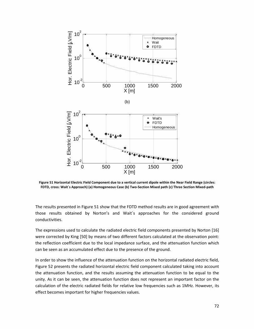
72
(b)
Figure 51 Horizontal Electric Field Component due to a vertical current dipole within the Near Field Range (circles: FDTD, cross: Wait´s Approach) (a) Homogeneous Case (b) Two-Section Mixed path (c) Three Section Mixed-path
The results presented in Figure 51 show that the FDTD method results are in good agreement with
those results obtained by Norton’s and Wait´s approaches for the considered ground
conductivities.
The expressions used to calculate the radiated electric field components presented by Norton [16]
were corrected by King [50] by means of two different factors calculated at the observation point:
the reflection coefficient due to the local impedance surface, and the attenuation function which
can be seen as an accumulated effect due to the presence of the ground.
In order to show the influence of the attenuation function on the horizontal radiated electric field,
Figure 52 presents the radiated horizontal electric field component calculated taking into account
the attenuation function, and the results assuming the attenuation function to be equal to the
unity. As it can be seen, the attenuation function does not represent an important factor on the
calculation of the electric radiated fields for relative low frequencies such as 1MHz. However, its
effect becomes important for higher frequencies values.
0 500 1000 1500 200010
-2
100
102
X [m]
Ho
r. E
lectr
ic F
ield
[ V
/m]
Homogeneous
Wait
FDTD
0 500 1000 1500 200010
-2
100
102
X [m]
Hor.
Ele
ctr
ic F
ield
[ V
/m]
Wait's
FDTD
Homogeneous
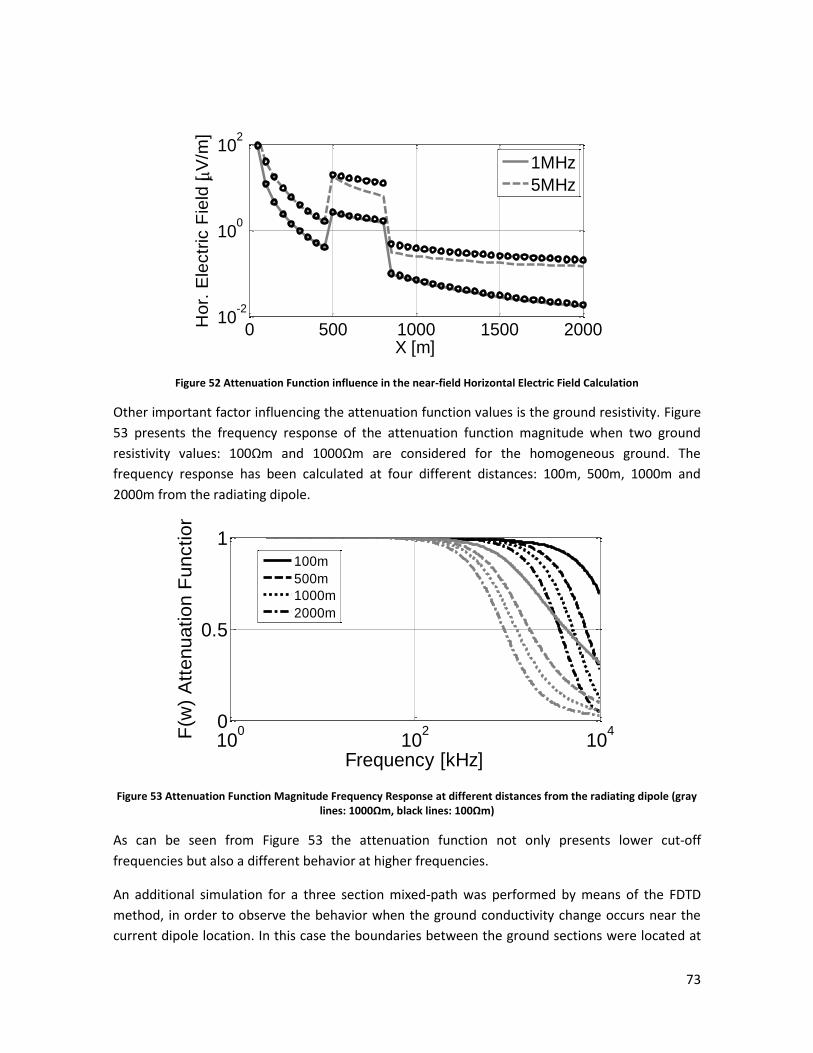
73
Figure 52 Attenuation Function influence in the near-field Horizontal Electric Field Calculation
Other important factor influencing the attenuation function values is the ground resistivity. Figure
53 presents the frequency response of the attenuation function magnitude when two ground
resistivity values: 100Ωm and 1000Ωm are considered for the homogeneous ground. The
frequency response has been calculated at four different distances: 100m, 500m, 1000m and
2000m from the radiating dipole.
Figure 53 Attenuation Function Magnitude Frequency Response at different distances from the radiating dipole (gray lines: 1000Ωm, black lines: 100Ωm)
As can be seen from Figure 53 the attenuation function not only presents lower cut-off
frequencies but also a different behavior at higher frequencies.
An additional simulation for a three section mixed-path was performed by means of the FDTD
method, in order to observe the behavior when the ground conductivity change occurs near the
current dipole location. In this case the boundaries between the ground sections were located at
0 500 1000 1500 200010
-2
100
102
X [m]
Ho
r. E
lectr
ic F
ield
[ V
/m]
1MHz
5MHz
100
102
104
0
0.5
1
Frequency [kHz]
F(w
) A
ttenuation F
unction
100m
500m
1000m
2000m

74
X1=250m and X2=450. A voltage dipole oscillating at 1MHz was placed at 1m above a mixed-path of
three sections; calculations of the e peak value were obtained once the steady-state of electric
field waveforms was achieved. The simulation in the FDTD was performed using regular meshing
with cubic cells with 5x5x2m3 in volumes. The total simulation volume space was 50x900x2000m3.
The computational domain was truncated by means of CPML boundaries.
(a)
Figure 54 Validity of the Wait formula for Mixed-Path of Three sections (a) Horizontal Electric Field
As can be seen from Figure 54 there is a good agreement between the results.
4.3.2 Radiated Fields over Irregular Ground
As it was discussed before, by means of the integral equation proposed by Ott [54] it is possible to
calculate the attenuation function in the far field region when there are irregular profiles along the
propagation path.
In order to evaluate this effect, a monochromatic oscillating voltage source with 50Ω in internal
resistance was placed at 2.5m above the ground and an obstacle with 50m in height and 400m in
length was included in the propagation path. A non-regular mesh FDTD simulation was performed
using the non-regular parabolic-meshing algorithm proposed in this thesis. The parameters were
set to 5m and 20m for the minimum and maximum spacing size respectively with a maximum
spacing-rate factor of 1. The Z-axis was meshed by regular discretization. The total space of
simulation was 4000x3000x1000m3 and the dipole was located at the coordinate X0=1000m,
Y0=1500m. In order to truncate the simulation space, absorbing 2nd order Liao´s boundaries were
implemented. The ground was simulated assuming 0.5Ωm in ground resistivity and εr=81 in
relative permittivity. Figure 55(a) shows the inclusion of the terrain irregularity in the FDTD
method. A finer mesh that can be seen near 1000m was included for a better representation of
the source.
200 400 600 800 10000
2
4
6
X [m]
Hor.
Ele
ctr
ic F
ield
[ V
/m]
Wait
FDTD
Sea=0.5m
Sea=0.5m
Land=500m

75
(a)
(b)
Figure 55 Irregular ground effect on radiated field in the near field (a) Ground Profile along the x-axis included into the FDTD method (b) Horizontal electric field from the current dipole location along an abrupt profile change for different oscillating frequencies (dashed: Homogeneous, black empty circle: 1MHz, gray filled circles: 5MHz , black filled circles:
10MHz)
As can be seen from Figure 55(b), the horizontal component of the radiated electric field increases
its magnitude before the terrain irregularity is reached. This effect is caused by the wave
reflections due to the presence of the ground step. In Figure 55(b) the electric field magnitude for
the homogeneous case is also shown in dashed line. As it can be seen for the 1MHz case, the
magnitude of the electric field changes when compared to the homogenous case value, then it
increases its magnitude closer to the ground step and once it is surpassed, the magnitude of the
electric field component returns to the homogeneous case value. A different behavior is observed
for the frequencies of 5MHz and 10MHz. As it can be seen, the first section of the path differs from
the homogeneous case due to the reflected wave magnitude and once the step ground is
overcome, the electric field magnitude presents different maxima and minima along the path. This
is mainly due to the interaction between the wave and the obstacle at the frequencies under
analysis.
0 500 1000 1500 2000
100
Distance X[m]
Ele
ctr
ic F
ield
[ V
/m]
Ground Step

76
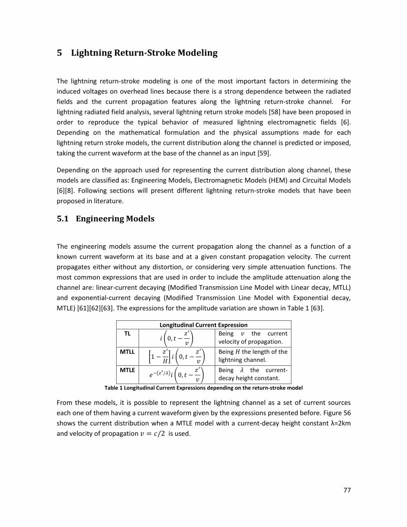
77
5 Lightning Return-Stroke Modeling
The lightning return-stroke modeling is one of the most important factors in determining the
induced voltages on overhead lines because there is a strong dependence between the radiated
fields and the current propagation features along the lightning return-stroke channel. For
lightning radiated field analysis, several lightning return stroke models [58] have been proposed in
order to reproduce the typical behavior of measured lightning electromagnetic fields [6].
Depending on the mathematical formulation and the physical assumptions made for each
lightning return stroke models, the current distribution along the channel is predicted or imposed,
taking the current waveform at the base of the channel as an input [59].
Depending on the approach used for representing the current distribution along channel, these
models are classified as: Engineering Models, Electromagnetic Models (HEM) and Circuital Models
[6][8]. Following sections will present different lightning return-stroke models that have been
proposed in literature.
5.1 Engineering Models
The engineering models assume the current propagation along the channel as a function of a
known current waveform at its base and at a given constant propagation velocity. The current
propagates either without any distortion, or considering very simple attenuation functions. The
most common expressions that are used in order to include the amplitude attenuation along the
channel are: linear-current decaying (Modified Transmission Line Model with Linear decay, MTLL)
and exponential-current decaying (Modified Transmission Line Model with Exponential decay,
MTLE) [61][62][63]. The expressions for the amplitude variation are shown in Table 1 [63].
Longitudinal Current Expression
TL (
)
Being the current velocity of propagation.
MTLL [
] (
)
Being the length of the lightning channel.
MTLE ( ) (
)
Being the current-decay height constant.
Table 1 Longitudinal Current Expressions depending on the return-stroke model
From these models, it is possible to represent the lightning channel as a set of current sources
each one of them having a current waveform given by the expressions presented before. Figure 56
shows the current distribution when a MTLE model with a current-decay height constant λ=2km
and velocity of propagation is used.
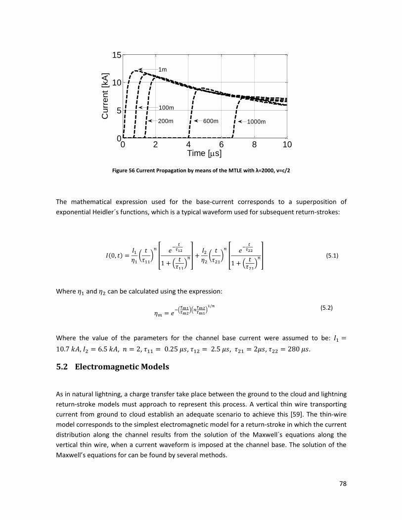
78
Figure 56 Current Propagation by means of the MTLE with λ=2000, v=c/2
The mathematical expression used for the base-current corresponds to a superposition of
exponential Heidler´s functions, which is a typical waveform used for subsequent return-strokes:
( )
(
*
[
(
)
]
(
*
[
(
)
] (5.1)
Where and can be calculated using the expression:
(
)(
)
(5.2)
Where the value of the parameters for the channel base current were assumed to be:
, , , , , .
5.2 Electromagnetic Models
As in natural lightning, a charge transfer take place between the ground to the cloud and lightning
return-stroke models must approach to represent this process. A vertical thin wire transporting
current from ground to cloud establish an adequate scenario to achieve this [59]. The thin-wire
model corresponds to the simplest electromagnetic model for a return-stroke in which the current
distribution along the channel results from the solution of the Maxwell´s equations along the
vertical thin wire, when a current waveform is imposed at the channel base. The solution of the
Maxwell’s equations for can be found by several methods.
0 2 4 6 8 100
5
10
15
Time [s]
Cu
rre
nt
[kA
]
600m 1000m200m
100m
1m
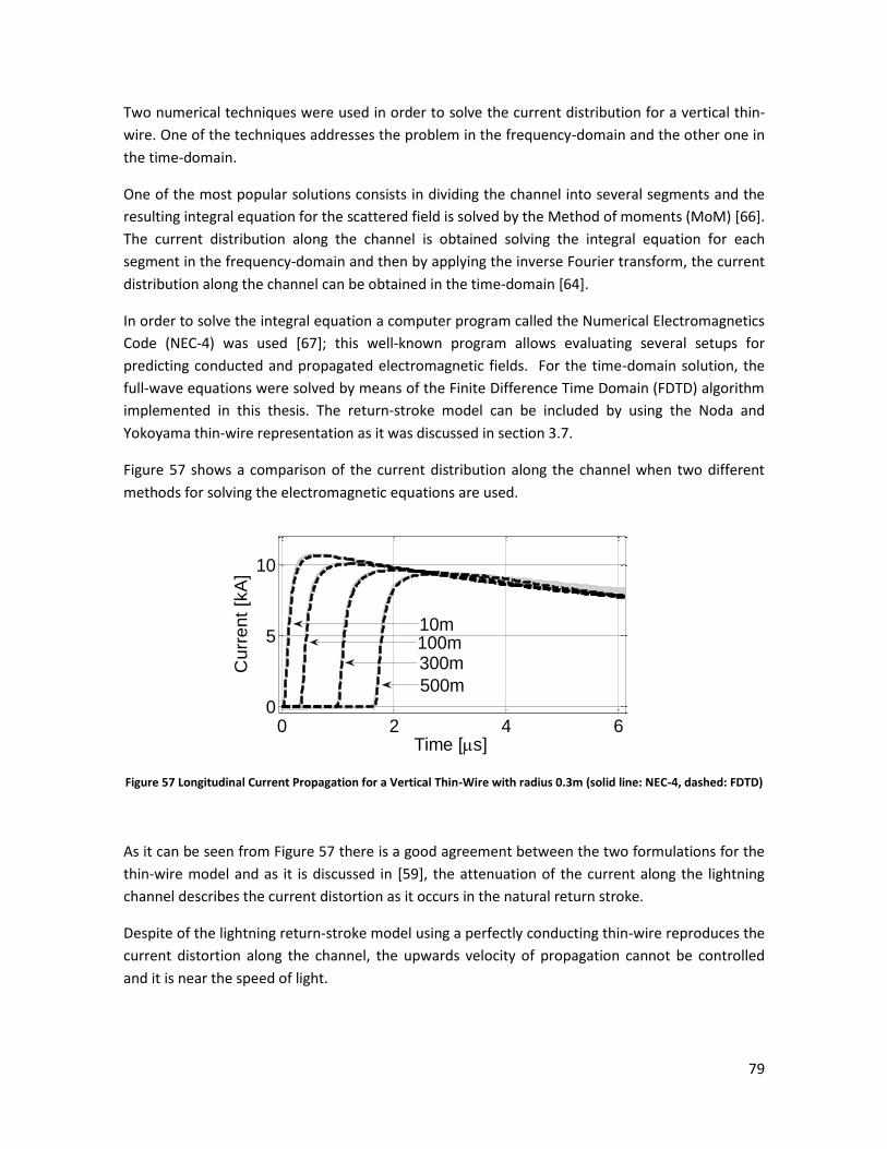
79
Two numerical techniques were used in order to solve the current distribution for a vertical thin-
wire. One of the techniques addresses the problem in the frequency-domain and the other one in
the time-domain.
One of the most popular solutions consists in dividing the channel into several segments and the
resulting integral equation for the scattered field is solved by the Method of moments (MoM) [66].
The current distribution along the channel is obtained solving the integral equation for each
segment in the frequency-domain and then by applying the inverse Fourier transform, the current
distribution along the channel can be obtained in the time-domain [64].
In order to solve the integral equation a computer program called the Numerical Electromagnetics
Code (NEC-4) was used [67]; this well-known program allows evaluating several setups for
predicting conducted and propagated electromagnetic fields. For the time-domain solution, the
full-wave equations were solved by means of the Finite Difference Time Domain (FDTD) algorithm
implemented in this thesis. The return-stroke model can be included by using the Noda and
Yokoyama thin-wire representation as it was discussed in section 3.7.
Figure 57 shows a comparison of the current distribution along the channel when two different
methods for solving the electromagnetic equations are used.
Figure 57 Longitudinal Current Propagation for a Vertical Thin-Wire with radius 0.3m (solid line: NEC-4, dashed: FDTD)
As it can be seen from Figure 57 there is a good agreement between the two formulations for the
thin-wire model and as it is discussed in [59], the attenuation of the current along the lightning
channel describes the current distortion as it occurs in the natural return stroke.
Despite of the lightning return-stroke model using a perfectly conducting thin-wire reproduces the
current distortion along the channel, the upwards velocity of propagation cannot be controlled
and it is near the speed of light.
0 2 4 60
5
10
Time [s]
Curr
ent
[kA
]
100m300m
500m
10m
80
5.3 Lightning Channel as a Loaded Thin-wire
In order to control the propagation velocity, distributed lumped elements that are able to storage
energy are included long the channel. By means of this approach the current propagation can be
delayed in time, achieving slower apparent phase-velocities [6][64].
In this case, a lightning channel having a radius of 0.23 m was placed in an air working volume of
60 60 2300 m3 divided into 1 1 10 m3 cells, above a perfectly conducting ground. The
channel was loaded with a series inductance L = 2µH/m and excited by a 10 m lumped current
source. Absorbing CPML boundaries were placed at the top and all sides of the working volume.
Figure 58 shows the calculated currents at different heights contrasted with those presented in
[6].
Figure 58 Current Distribution along a Thin-Wire inductance-loaded (Solid line: FDTD implementation, circles line: Results presented in [6]).
As it can be seen from Figure 58, the calculated current distribution along the channel exhibits
distortion as in the perfectly conducting thin-wire model, but in addition the velocity of
propagation is controlled about 0.6 times the speed of light.
The thin wire model can be also loaded with a series resistive-inductive per unit length in order to
reproduce not only the phase-velocity of the propagating current as it was shown with the
inductive load, but also to obtain more attenuation whereas the current propagates.
In order to analyze the effect of loading the thin-wire by RL-series load, a simulation in NEC-4 by
means of a wire loaded by lumped RL series branches and a thin-wire implementation into the
FDTD method was performed. The thin-wire had 2000m in length and 0.23m in radius. In order to
obtain a current propagation velocity of near one-third of the speed of light a series resistive-
inductive (RL) load value of 1Ω/m and 2µH/m was used. The current waveform used was the one
proposed by Chen as illustrated in [10].
0 1 2 3 4 50
5
10
15
20
Time [s]
Curr
ent
[kA
]
0m150m
300m
600m
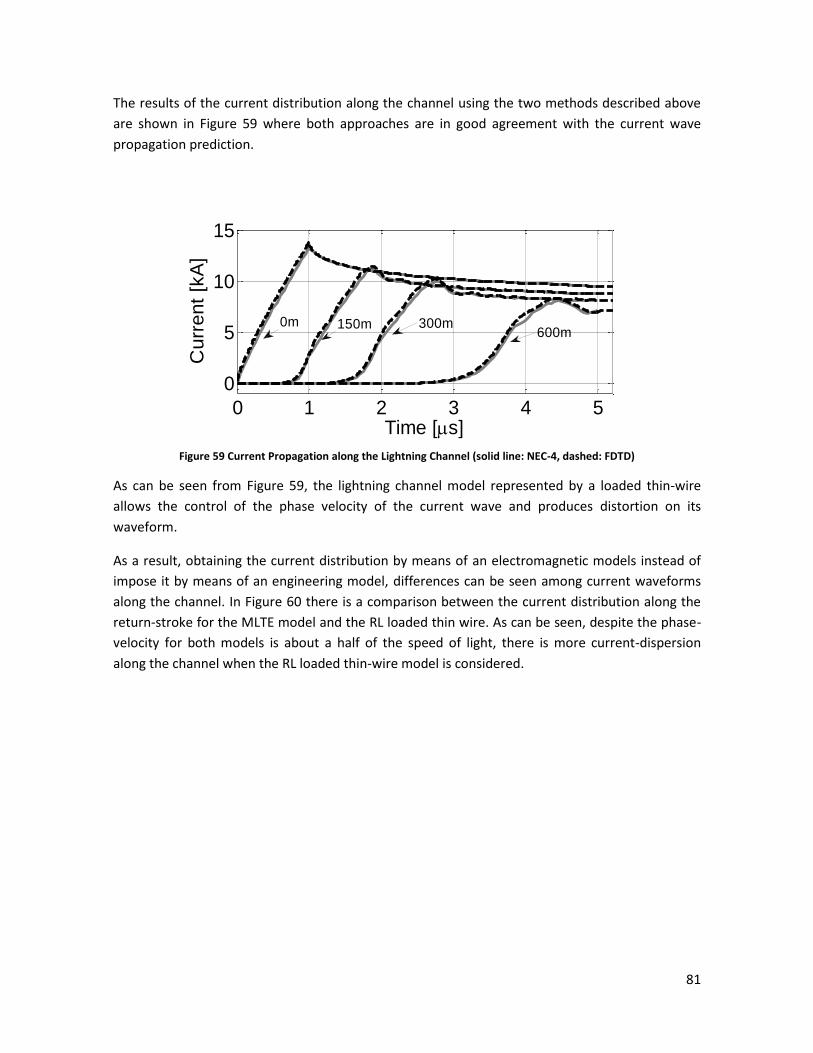
81
The results of the current distribution along the channel using the two methods described above
are shown in Figure 59 where both approaches are in good agreement with the current wave
propagation prediction.
Figure 59 Current Propagation along the Lightning Channel (solid line: NEC-4, dashed: FDTD)
As can be seen from Figure 59, the lightning channel model represented by a loaded thin-wire
allows the control of the phase velocity of the current wave and produces distortion on its
waveform.
As a result, obtaining the current distribution by means of an electromagnetic models instead of
impose it by means of an engineering model, differences can be seen among current waveforms
along the channel. In Figure 60 there is a comparison between the current distribution along the
return-stroke for the MLTE model and the RL loaded thin wire. As can be seen, despite the phase-
velocity for both models is about a half of the speed of light, there is more current-dispersion
along the channel when the RL loaded thin-wire model is considered.
0 1 2 3 4 5
0
5
10
15
Time [s]
Curr
ent
[kA
]
150m0m 300m600m
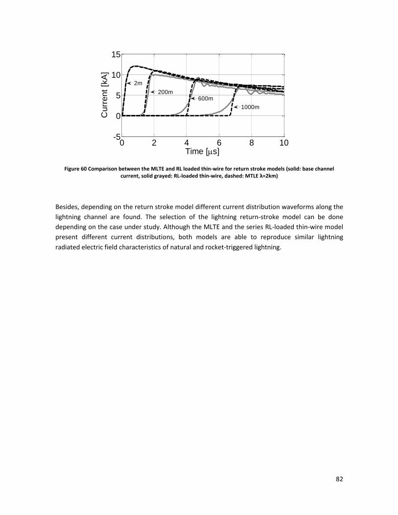
82
Figure 60 Comparison between the MLTE and RL loaded thin-wire for return stroke models (solid: base channel current, solid grayed: RL-loaded thin-wire, dashed: MTLE λ=2km)
Besides, depending on the return stroke model different current distribution waveforms along the
lightning channel are found. The selection of the lightning return-stroke model can be done
depending on the case under study. Although the MLTE and the series RL-loaded thin-wire model
present different current distributions, both models are able to reproduce similar lightning
radiated electric field characteristics of natural and rocket-triggered lightning.
0 2 4 6 8 10-5
0
5
10
15
Time [s]
Cu
rre
nt
[kA
]1000m
600m200m
2m

83
6 Propagation Path Effects on Lightning Radiated Fields
This section addresses the effects of the presence of different ground structures on the lightning-
radiated fields. As it was presented before for a current dipole, the characteristics of the
propagation path can affect the electric radiated fields in a considerable magnitude. These effects
were analyzed not only in the far-field region but also it was demonstrated to have an important
contribution in the near field region.
As it was shown before, the lightning return-stroke channel can be modeled by means of several
approaches. All of those models reproduce the most important characteristics of the natural
return-stroke current distribution and any could be used for calculating lightning radiated fields.
As it was discussed in section 5, the characteristics of the current propagation in a natural return-
stroke can be reproduced when electromagnetic models are used.
Based on this approach, the results discussed before for a vertical-current dipole above different
ground structures in the frequency domain can be extended, using the superposition theorem, by
means of a set of vertical-current dipoles along the channel and the evaluation of its contribution
at the observation point. Once the frequency response at an evaluation point has been calculated
including all the sources that represent the lightning channel, the inverse Fourier transform can be
used in order to determine the time-domain waveform for a determined channel-base current.
6.1 Perfectly Conducting Ground
The perfectly conducting ground effect can be taken into account by the theoretical formulation
based on the image theory method. The perfectly conducting ground can be seen as a reference
condition for cases where the lossy, inhomogeneous and irregular ground conditions are present.
A comparison between the theoretical predictions and those results calculated by a full-wave
solution for the near field region were carried out in order to validate the FDTD method for
calculating lightning radiated fields from return-stroke modeled by means of a RL-loaded thin-
wire. Using the FDTD implementation with non-regular meshing, a more detailed mesh was
specified near the lightning channel location whereas a coarser domain was assumed for the rest
of the region.
The minimum spacing size was assumed to be 5m. The maximum spacing was about 50m for the x
and y direction and 7.5m for the z direction. The z-direction domain was meshed as regular up to
150m above the ground interface. The non-regular mesh was calculated by means of the proposed
parabolic meshing using an attenuation factor α=0.1 for soft spacing change along the z-axis and
α=0.5 and for the x and y axis. Figure 61 presents the mesh distribution for the simulation
scenario. The lightning channel modeled as a loaded thin-wire was placed at the coordinate
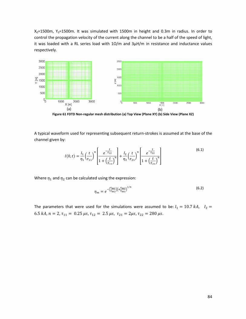
84
X0=1500m, Y0=1500m. It was simulated with 1500m in height and 0.3m in radius. In order to
control the propagation velocity of the current along the channel to be a half of the speed of light,
it was loaded with a RL series load with 1Ω/m and 3μH/m in resistance and inductance values
respectively.
(a)
(b)
Figure 61 FDTD Non-regular mesh distribution (a) Top View (Plane XY) (b) Side View (Plane XZ)
A typical waveform used for representing subsequent return-strokes is assumed at the base of the
channel given by:
( )
(
*
[
(
)
]
(
*
[
(
)
]
(6.1)
Where and can be calculated using the expression:
(
)(
)
(6.2)
The parameters that were used for the simulations were assumed to be:
, , , , , .

85
Figure 62 presents the current distribution along the lightning channel for both different
approaches, one of them is based on the antenna theory model with fixed inductive load and
when the RL loaded thin-wire model is considered into a non-regular mesh FDTD simulation. As it
can be observed, the current distributions obtained from the FDTD method agree well with those
obtained from the MoM solution using the NEC-4 code.
Figure 62 Current Distribution along the Lightning Channel RL loaded Return-Stroke model (solid grayed: NEC-4, dashed line: FDTD-Thin Wire RL loaded)
In Figure 63 there is a comparison for the horizontal electric field calculation by means of the FDTD
in the near field region and those results using the theoretical calculation by means of the image
theory. Two different distances from the lightning channel base to the observation point were
analyzed. Range I: distances closer than 200m and Range II: distances longer than 500m.
(a)
(b)
Figure 63 Lightning Radiated Fields above Perfectly Conducting Ground, Horizontal Electric Field (Solid Line: Theoretical, Dashed Line: FDTD) (a) Hor. Electric Field Range I (closer distances than 200m to the Channel Base) (b)
Hor. Electric Field Range II (longer distances than 500m to the Channel Base)
As can be seen from Figure 63 the FDTD results are in a good agreement with those using the
theoretical calculation. The maximum error between both results is about 2%. This is a tolerable
0 2 4 6 8 10-5
0
5
10
15
Cu
rre
nt
[kA
]
time [s]
7m 107m 377m
527m 901m
1125m
0 2 4 6 8 10-2
0
2
4
6
Time [s]
Hor.
Ele
ctr
ic F
ield
[kV
/m]
58.7m107.5m
152.5m
0 2 4 6 8 10-0.02
0
0.02
0.04
0.06
Time [s]
Hor.
Ele
ctr
ic F
ield
[kV
/m]
527.5m
977m
677.5m

86
error taking into account the considerable decreasing on the total simulation time and the
maximum space volume when a non-regular mesh is used.
6.2 Homogeneous Lossy Ground
The presence of lossy ground has been demonstrated to be a very important factor in lighting
radiated field waveforms, especially for the horizontal electric field component within the near
field region.
Norton´s approximation has been tested for lightning radiated field calculations in multiple
scenarios of distance and ground conductivities, concluding about its validity in the near-field only
when relatively good ground conductivities values are present. Even for some cases, the Norton´s
approximation provides reasonable results for ground resistivity values lower than 1000Ωm and
for distances within 50m up to 200m from the channel base. It has been also showed that the
Norton´s approach leads to better results in the case of subsequent return strokes.
In order to validate the lightning radiated fields. Figure 64 presents a comparison between the
rigorous solution of the Sommerfeld´s equations taken from [20] and the Norton´s approach
implemented in this thesis for the horizontal electric field component above a homogeneous
ground with a resistivity ρ=1000Ωm at 200m from the lightning channel. The return-stroke current
corresponds to a typical subsequent stroke and the same parameters presented in [15] were used.
Figure 64 Horizontal Electric field at 10m height above a lossy ground of resistivity 1000Ωm at a distance of 200m from the stroke modeled by MLTE (dashed: Norton Approach, circles: Sommerfeld’s taken from [20])
As can be seen from Figure 64 Norton´s approach is in well agree with the rigorous solution of the
Sommerfeld´s integrals as most of the principal characteristics of the radiated waveform are
0 2 4 6 8 10-200
0
200
400
Time [s]
Hor.
Ele
ctr
ic F
ield
[V
/m]

87
reproduced. The negative excursion that is present in the horizontal electric field component has
been shown to be highly dependent on the resistivity of the ground and the vertical electric field
component.
In order to analyze the effect of the ground resistivity on the lightning radiated field magnitudes
and waveforms, a set of simulations with different ground conductivities were performed by using
the Norton´s approach. In Figure 65 a comparison for the electric radiated field components for
10Ωm, 100Ωm and 1000Ωm resistivity values is presented. The return stroke was modeled by a
straight wire loaded with a lumped RL load of 1Ω/m in resistance and 3μH/m in inductance
respectively. The current distribution along the channel was obtained by means of the antenna
theory approach by using the NEC-4 code as it was discussed in section 5.3. The electric fields were
calculated at 10m above the ground.
As it can be seen from Figure 65(a), the vertical component of the radiated electric field is less
affected by the resistivity ground values than the horizontal one. Figure 65(b) and Figure 65(c)
shows that the waveform shape of the horizontal component is highly affected by the resistivity
changes. The negative excursion is the most evident distortion especially for distances greater
than 500m from the lightning channel base. However, for all the cases radiated electric fields
tends to the same maximum value.

88
(a)
(b)
(b)
Figure 65 Radiated Electric Fields above different Ground Resistivity values (a) Vertical Electric Field (b) Horizontal Electric Field for distances closer than 200m (c) Horizontal Electric Field for distances further than 500m
As it was presented in section 5, the current distribution along the channel depends on the
lightning channel model. In order to verify the influence on the lightning radiated fields due to the
current distribution along the channel, a comparison between the horizontal and vertical
component due to a MLTE model and RL-Thin-wire was performed. For the lightning channel
model represented by the loaded vertical wire the current distribution along the channel was
calculated by the NEC-4, however the radiated fields are in both cases calculated by the Norton´s
approach. In Figure 66 there is a comparison between the current distribution along the channel
and their radiated fields above lossy ground with 1000Ωm in resistivity and 10ε0 in permittivity
when two different lightning return-stroke models are used, the MLTE model with λ=2km and the
RL loaded thin wire with 1Ω/m in resistance and 3μH/m in inductance.
0 2 4 6 8 10-20
-15
-10
-5
0
Time [s]
Ve
r. E
lectr
ic F
ield
[kV
/m]
10m
100m
1000m
0 2 4 6 8 10-1000
0
1000
2000
Time [s]
Hor.
Ele
ctr
ic F
ield
[V
/m]
10m
100m
1000m
200m
100m
0 2 4 6 8 10-100
-50
0
50
100
Time [s]
Hor.
Ele
ctr
ic F
ield
[V
/m]
10m
100m
1000m
500m
1000m

89
(a)
(b)
(b)
Figure 66 Horizontal Electric Field Component with different lightning return-stroke model (solid: RL Thin-Wire, dashed: MLTE) (a) Current distribution along the Channel (b) Electric Field Component at distances closer than 200m (c) Electric Field Component at distances further than 500m
As can be seen from the comparison presented in Figure 66, the waveforms of the radiated fields
are similar to each other but it can be also found some important differences at closer distances
from the lightning channel base. For further distances from the lightning channel base the
0 2 4 6 8 10-5
0
5
10
15
Time [s]
Curr
ent
[kA
]
1000m
600m200m
2m
0 2 4 6 8 10
0
1000
2000
3000
4000
Time [s]
Hor.
Ele
ctr
ic F
ield
[V
/m]
0 0.5 1 1.5-200
-100
0
100
200m100m
0 2 4 6 8 10-100
-50
0
50
Time [s]
Hor.
Ele
ctr
ic F
ield
[V
/m]
500m
1000m

90
negative excursion is the most affected characteristic of the waveform by the current distribution
[69].
As it has been shown by several authors, Norton´s approach can be applied for some near field
situations of lightning radiated fields. However, this approach is not valid for all the distance
ranges and its intrinsic assumption of cylindrical problem space symmetry is normally invalid for
general cases of lightning induced voltages. The FDTD method can be used for those situations
where the Norton’s approach assumptions are not valid or more general simulation scenarios
must be simulated.
In [70] a FDTD simulation with a fine mesh was performed in order to validate the popular CR
formula for the horizontal radiated field above lossy ground [21][22]. Figure 67 presents a
comparison between the results presented in [70] by a very fine-mesh FDTD and the Norton´s
approach implemented in this thesis. The comparison is presented for the near field range at
100m and 1000m from the lightning channel base.
Figure 67 Horizontal Electric field at 10m height above a lossy ground of resistivity 100Ωm at two-different distances
from the channel modeled by RL Loaded Thin-Wire (a) at distance of 100m (b) at distance of 1km (dashed: Norton Approach, circles: FDTD taken from [70])
In order to validate the Norton´s approach for calculating lightning radiated fields above a relative
high ground resistivity (ρ=1000Ωm), a simulation set-up using a full-wave solution by means of the
FDTD method with non-regular mesh was performed.
The lightning channel was modeled by means of the MTLE model assuming λ=2km and a velocity
of propagation of c/2 and 1500m in height. The ground conductivity was assumed to be 1000Ωm
along with a Non-regular mesh with a maximum space discretization of 17.5m in the coarser
domain. In the region of interest a delta space of 5m was used. In Z-directed coordinates regular
spacing was considered and the lightning channel was placed in the center of the XY plane.
Radiated fields were calculated along the x-axis in order to coincide with those radial electric fields
calculated from the Norton´s approach. Figure 68 shows the non-regular mesh used for the
simulation.
0 2 4 6 8 10-1000
0
1000
2000
Time [s]
Ho
r. E
lectr
ic F
ield
[V
/m]
0 2 4 6 8 10-20
-10
0
10
Time [s]
H
or.
Ele
ctr
ic F
ield
[kV
/m]
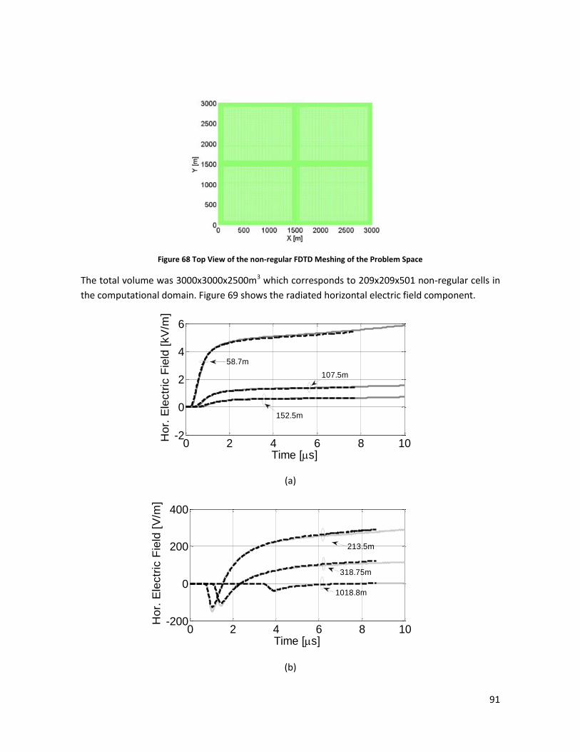
91
Figure 68 Top View of the non-regular FDTD Meshing of the Problem Space
The total volume was 3000x3000x2500m3 which corresponds to 209x209x501 non-regular cells in
the computational domain. Figure 69 shows the radiated horizontal electric field component.
(a)
(b)
0 2 4 6 8 10-2
0
2
4
6
Time [s]
Ho
r. E
lectr
ic F
ield
[kV
/m]
58.7m
152.5m
107.5m
0 2 4 6 8 10-200
0
200
400
Time [s]
Ho
r. E
lectr
ic F
ield
[V
/m]
1018.8m
318.75m
213.5m
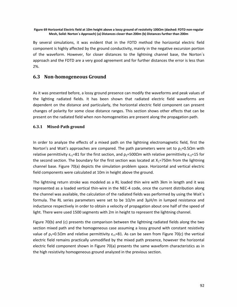
92
Figure 69 Horizontal Electric field at 10m height above a lossy ground of resistivity 100Ωm (dashed: FDTD non-regular Mesh, Solid: Norton´s Approach) (a) Distances closer than 200m (b) Distances further than 200m
By several simulations, it was evident that in the FDTD method the horizontal electric field
component is highly affected by the ground conductivity, mainly in the negative excursion portion
of the waveform. However, for closer distances to the lightning channel base, the Norton´s
approach and the FDTD are a very good agreement and for further distances the error is less than
2%.
6.3 Non-homogeneous Ground
As it was presented before, a lossy ground presence can modify the waveforms and peak values of
the lighting radiated fields. It has been shown that radiated electric field waveforms are
dependent on the distance and particularly, the horizontal electric field component can present
changes of polarity for some close distance ranges. This section shows other effects that can be
present on the radiated field when non-homogeneities are present along the propagation path.
6.3.1 Mixed-Path ground
In order to analyze the effects of a mixed path on the lightning electromagnetic field, first the
Norton’s and Wait’s approaches are compared. The path parameters were set to ρ1=0.5Ωm with
relative permittivity εr1=81 for the first section, and ρ2=500Ωm with relative permittivity εr2=15 for
the second section. The boundary for the first section was located at X1=750m from the lightning
channel base. Figure 70(a) depicts the simulation problem space. Horizontal and vertical electric
field components were calculated at 10m in height above the ground.
The lightning return stroke was modeled as a RL loaded thin wire with 3km in length and it was
represented as a loaded vertical thin-wire in the NEC-4 code, once the current distribution along
the channel was available, the calculation of the radiated fields was performed by using the Wait´s
formula. The RL series parameters were set to be 1Ω/m and 3μH/m in lumped resistance and
inductance respectively in order to obtain a velocity of propagation about one half of the speed of
light. There were used 1500 segments with 2m in height to represent the lightning channel.
Figure 70(b) and (c) presents the comparison between the lightning radiated fields along the two
section mixed path and the homogeneous case assuming a lossy ground with constant resistivity
value of ρ1=0.5Ωm and relative permittivity εr1=81. As can be seen from Figure 70(c) the vertical
electric field remains practically unmodified by the mixed path presence, however the horizontal
electric field component shown in Figure 70(a) presents the same waveform characteristics as in
the high resistivity homogeneous ground analyzed in the previous section.
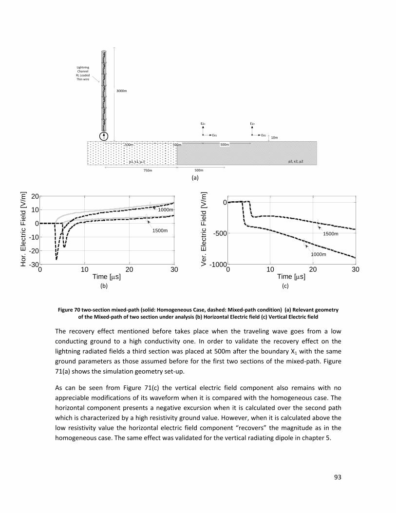
93
750m
ρ1, ε1, μ 1
Lightning Channel
RL Loaded Thin wire
ρ2, ε2, μ2
500m
500m500m 500m
Ex1 Ex2
Ez1 Ez2
10m
3000m
(a)
(b)
(c)
Figure 70 two-section mixed-path (solid: Homogeneous Case, dashed: Mixed-path condition) (a) Relevant geometry of the Mixed-path of two section under analysis (b) Horizontal Electric field (c) Vertical Electric field
The recovery effect mentioned before takes place when the traveling wave goes from a low
conducting ground to a high conductivity one. In order to validate the recovery effect on the
lightning radiated fields a third section was placed at 500m after the boundary X1 with the same
ground parameters as those assumed before for the first two sections of the mixed-path. Figure
71(a) shows the simulation geometry set-up.
As can be seen from Figure 71(c) the vertical electric field component also remains with no
appreciable modifications of its waveform when it is compared with the homogeneous case. The
horizontal component presents a negative excursion when it is calculated over the second path
which is characterized by a high resistivity ground value. However, when it is calculated above the
low resistivity value the horizontal electric field component “recovers” the magnitude as in the
homogeneous case. The same effect was validated for the vertical radiating dipole in chapter 5.
0 10 20 30-30
-20
-10
0
10
20
Time [s]
Hor.
Ele
ctr
ic F
ield
[V
/m]
1000m
1500m
0 10 20 30-1000
-500
0
Time [s]
Ve
r. E
lectr
ic F
ield
[V
/m]
1500m
1000m

94
750m
ρ1, ε1, μ 1
Lightning Channel
RL Loaded Thin wire
ρ2, ε2, μ2 ρ1, ε1, μ 1
500m
500m500m 500m
Ex1 Ex2
Ez1 Ez2
10m
3000m
(a)
(b)
(c)
Figure 71 Mixed-Path of three sections for lightning radiated fields (solid: Homogeneous Case, dashed: Mixed-path condition) (a) Relevant geometry of the Mixed-path of three sections under analysis (b) Horizontal Electric field (c)
Vertical Electric field
As it was discussed in previous sections, the Wait´s approach for the propagation along a mixed-
path sections is based on several considerations that in general cannot be assumed on several
scenarios. The FDTD method allows simulating multi mixed-path sections without specific
assumptions about the section lengths and geometric symmetry. In order to compare the results
obtained with the Wait approach with those obtained with the FDTD method, a simulation set-up
of a mixed-path was performed and its results were compared with those calculated by means of
the Wait´s formulas.
The Mixed Path was located at 205m from the lightning channel base and electric field
components have been calculated along the propagation path at 10m above the ground. Figure
72(a) depicts the simulation scenario. The lightning channel was simulated in the FDTD by means
0 10 20 30-40
-20
0
20
Time [s]
Ho
r. E
lectr
ic F
ield
[V
/m]
1000m
1500m
0 10 20 30-1000
-500
0
Time [s]
Ve
r. E
lectr
ic F
ield
[V
/m]
1500m
1000m

95
of a MTLE model with a velocity of propagation set to be one half of the speed of light and
attenuation factor λ=2km. The lightning channel length was assumed to be 1.5km in length.
Ex1 Ex2
σ1, ε1, μ 1σ2, ε2, μ2
Lighting Channel MTLE
Representation
1.5kmλ=2000v=c/2
205m
310m
1010m
(a)
(b)
(c)
Figure 72 Lightning Radiated Fields Mixed-Path of Two-Section calculated by the FDTD method. Case 1 (Gray line): 10Ωm / 1000Ωm, Case 2 (Black line): 1000Ωm / 10Ωm (a) Simulation Set-Up (b) Horizontal Electric Field (c) Vertical
Electric Field
0 2 4 6 8-0.1
-0.05
0
0.05
0.1
Hor.
Ele
ctr
ic F
ield
[kV
/m]
time [s]
1010m
310m
0 2 4 6 8
-3
-2
-1
0
Ver.
Ele
ctr
ic F
ield
[kV
/m]
time [s]
1010m
310m

96
As it can be seen from Figure 72(b) and Figure 72(c), the change of ground conductivity affects
mainly the horizontal electric field component. The vertical electric field component can be
assumed as undisturbed by the ground conductivity changes; this result is in agreement with the
analysis presented in section 6.2 where different ground conductivity and distances from the
channel base were considered. As in Figure 70, similar waveforms for the horizontal electric field
can be seen in both simulations.
In order to validate the effects of the mixed-path on the lightning radiated fields and the validity of
the Wait´s formulas within the near field range, the same simulation set-up proposed in Figure
72(a) was used for the calculation of the radiated fields by using the Wait´s formulas and the
results are compared with those presented in Figure 72(b) and Figure 72(c) by means of the FDTD.
(a)
(b)
(c)
(d)
Figure 73 Radiated Electric Field Components along a Mixed-Path of two-sections. (Dashed Line: Wait’s Formulas, Solid Line: FDTD Method) Case 1: 10 Ωm / 1000 Ωm (a) Hor. Electric Field (b) Ver. Electric Field, Case 2: 1000 Ωm /
10Ωm (c) Hor. Electric Field (d) Ver. Electric Field Case
As it can be seen in Figure 73(b) and Figure 73(d) the vertical electric field can be well reproduced
by the Wait´s formula within the near field range. In both cases , the vertical electric field
component prediction by the Wait´s formula agrees with the FDTD predictions with a relative
error under the 1%. This validity has been also examined recently in [58] with different channel-
base current waveforms for first and subsequent return stroke representations showing
0 2 4 6 8
-0.1
-0.05
0
0.05
0.1
Ho
r. E
lectr
ic F
ield
[kV
/m]
time [s]
310m
1010m
0 2 4 6 8
-3
-2
-1
0
Time [s]
Ver.
Ele
ctr
ic F
ield
[kV
/m]
1010m
310m
0 2 4 6 8
0
0.05
0.1
0.15
Time [s]
Hor.
Ele
ctr
ic F
ield
[kV
/m]
310m
1010m
0 2 4 6 8-3
-2
-1
0
Time [s]
Ver.
Ele
ctr
ic F
ield
[kV
/m]
310m
1010m

97
reasonably accuracy for predicting the vertical electric field component at closer distances.
However, Figure 73(a) and Figure 73(c) present important differences for the horizontal electric
field calculation, especially for the case when the traveling electromagnetic wave goes from a
lower conductivity ground to a higher one.
As it was presented in section 4.2.2 the Wait´s formula is valid for the far field range only and the
vertical inhomogeneity boundary must be far enough from the radiating dipole. The differences
observed in the horizontal electric field component can be caused by those approximations. As it
can be seen from Figure 73(a) the results predicted by the Wait´s formula are in good agreement
for most of the simulation time interval except for the peak calculation which is overestimated by
the Wait’s approach.

98
7 Lightning Induced Over-voltages
This section deals with the induced over-voltage calculation on the overhead lines due to a nearby
lightning strike. At this point several effects on the lightning radiated fields due to the propagation
path characteristics have been analyzed. One of the most common applications on the study of
lightning radiated fields is the induced over-voltages on overhead lines, that is why the
understanding of the propagation path effects on the lightning radiated fields are highly important
to be characterized and accurately calculated in order to determine their effects on power quality
due to the induced voltages adverse effects.
The electromagnetic coupling between lightning radiated fields and the overhead line has been
typically analyzed by the incident-scattered field formulation. One of the most popular is that
proposed by Agrawal [2], where the transmission homogeneous line equations are modified by
external electromagnetic source due to the incident field. By means of this coupling model, the
vertical and horizontal component of the radiated electric field can be included into the
transmission line equations as external sources in a straightforward way. The incident-scattered
field formulation has been one of the most used methods to calculate lightning induced voltages,
in this formulation the induced voltages can be calculated using the electric field components [71]
or using the magnetic field components [72] depending directly on the assumptions made for the
lightning radiated fields calculation [73].
As it has been shown in previous sections, all of the approaches for the lightning radiated field
calculations are based on far-field assumptions and cylindrical symmetry which is not adequate for
most of the practical scenarios. Although, the far-field approaches can be used showing a good
agreement with experimental results [23][23].
This section analyzes different effects on the lightning induced voltages that cannot be addressed
by the approaches presented in literature and discussed in previous sections. To achieve this, the
FDTD method will be used combined with the non-regular meshing algorithms developed in this
thesis in order to represent typical configurations of overhead lines. As several simulation
scenarios are not available to be compared with existent results in literature, a basis scenario of a
flat lossy ground will be simulated in order to compare the effects on the lightning induced
voltages due to the inhomogeneities and non-uniformities of the ground.
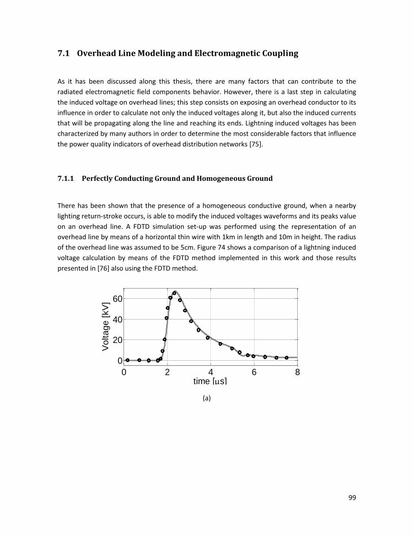
99
7.1 Overhead Line Modeling and Electromagnetic Coupling
As it has been discussed along this thesis, there are many factors that can contribute to the
radiated electromagnetic field components behavior. However, there is a last step in calculating
the induced voltage on overhead lines; this step consists on exposing an overhead conductor to its
influence in order to calculate not only the induced voltages along it, but also the induced currents
that will be propagating along the line and reaching its ends. Lightning induced voltages has been
characterized by many authors in order to determine the most considerable factors that influence
the power quality indicators of overhead distribution networks [75].
7.1.1 Perfectly Conducting Ground and Homogeneous Ground
There has been shown that the presence of a homogeneous conductive ground, when a nearby
lighting return-stroke occurs, is able to modify the induced voltages waveforms and its peaks value
on an overhead line. A FDTD simulation set-up was performed using the representation of an
overhead line by means of a horizontal thin wire with 1km in length and 10m in height. The radius
of the overhead line was assumed to be 5cm. Figure 74 shows a comparison of a lightning induced
voltage calculation by means of the FDTD method implemented in this work and those results
presented in [76] also using the FDTD method.
(a)
0 2 4 6 8
0
20
40
60
time [s]
Vo
lta
ge [
kV
]

100
(b)
Figure 74 Calculated Induced Voltages on a 1km at 50m from the lightning strike (solid: FDTD, circles: presented in [76])
As it can be seen from Figure 74, the induced voltages are highly modified by the presence of a
finite conducting ground. Figure 74(a) presents the induced voltage assuming a perfectly
conducting ground and when these results are compared with those obtained for a lossy ground of
1000 Ωm shown in Figure 74(b), several differences in the waveform can be evidenced.
One of the most interesting results between Figure 74(a) and Figure 74(b) is that the presence of
the lossy ground can include a change the polarity of the induced voltage. This effect is caused by
the incident lightning radiated field waveform, especially due to the same change of polarity
present in the horizontal electric field. As it was presented in section 6.2, the lossy ground affects
mainly the horizontal electric field component and its resulting waveforms exhibit a negative
excursion for the first time instants. These polarity changes interact with the overhead line
yielding to induced voltages having a similar behavior.
7.1.2 In-homogeneous Ground
This section pretends to evaluate some of the effects of the inhomogeneities on the lightning
induced voltages.
7.1.2.1 Mixed-Path condition
The Mixed path condition was demonstrated to contribute representatively to the lighting
radiated field waveforms in section 6.3.1. Hence, the induced voltages waveforms related to those
incident fields will be also affected. In order to analyze the effects of the non-homogenous ground
on induced voltage calculations, an overhead transmission line illuminated by the electromagnetic
field produced by a lightning channel striking at 50 m from one of its ends is considered. The
calculation was performed using a regular mesh implementation of the FDTD method as
0 2 4 6 8-20
0
20
40
Voltage [
kV
]
time [s]
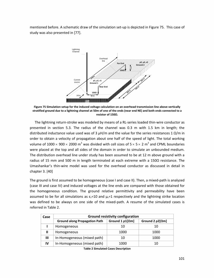
101
mentioned before. A schematic draw of the simulation set-up is depicted in Figure 75. This case of
study was also presented in [77].
50 m
250 m
250 m
12
m
Lightning
Channel
Current
source
Overhead
line
ρ1, μ1, ε1
ρ2, μ2, ε2
150Ω
150Ω
500 m
900m
1000m
200m
Ground 1
Ground 2
Near End
Far End
Figure 75 Simulation setup for the induced voltage calculation on an overhead transmission line above vertically stratified ground due to a lightning channel at 50m of one of the ends (near end NE) and both ends connected to a
resistor of 150Ω.
The lightning return-stroke was modeled by means of a RL-series loaded thin-wire conductor as
presented in section 5.3. The radius of the channel was 0.3 m with 1.5 km in length; the
distributed inductance value used was of 3 µH/m and the value for the series resistances 1 Ω/m in
order to obtain a velocity of propagation about one half of the speed of light. The total working
volume of 1000 900 2000 m3 was divided with cell sizes of 5 5 2 m3 and CPML boundaries
were placed at the top and all sides of the domain in order to simulate an unbounded medium.
The distribution overhead line under study has been assumed to be at 12 m above ground with a
radius of 15 mm and 500 m in length terminated at each extreme with a 150Ω resistance. The
Umashankar’s thin-wire model was used for the overhead conductor as discussed in detail in
chapter 3. [40]
The ground is first assumed to be homogeneous (case I and case II). Then, a mixed-path is analyzed
(case III and case IV) and induced voltages at the line ends are compared with those obtained for
the homogeneous condition. The ground relative permittivity and permeability have been
assumed to be for all simulations as εr=10 and µr=1 respectively and the lightning strike location
was defined to be always on one side of the mixed-path. A resume of the simulated cases is
referred in Table 2.
Case Ground resistivity configuration
Ground along Propagation Path Ground 1 ρ1*Ωm+ Ground 2 ρ2*Ωm+
I Homogeneous 10 10
II Homogeneous 1000 1000
III In-Homogeneous (mixed path) 10 1000
IV In-Homogeneous (mixed path) 1000 10
Table 2 Simulated Cases Description

102
Figure 76 shows the horizontal electric field components for the second section of the mixed-
paths considered in the simulation. As it is shown in Figure 76(b), the presence of the mixed path
section does not influence in a representative way the vertical electric field component. However,
the horizontal electric field component is markedly affected by the mixed-path structure.
(a)
Figure 76 Electric field components above the second mixed path section (Black: 10 Ωm / 1000 Ωm case, Gray 1000 Ωm / 10 Ωm case) (a) Horizontal electric field over a mixed-path ground (b) Vertical electric field over a mixed-path
ground
As it can be seen from Figure 76(a) for case III, when the wave propagates initially along a ground
of 10 Ωm it suffers almost no distortion when compared to a propagation along a perfectly
conducting ground. Once it starts to propagate along the 1000 Ωm ground, it is strongly distorted
changing its polarity for the first microseconds (black line). On the opposite case (case IV), the
wave starts to propagate above a highly lossy ground but when it enters to the 10 Ωm section, it
recovers the features of a propagation above an almost ideal ground. This leads to the differences
between the induced voltages calculated for the homogeneous and the in-homogeneous cases as
is presented in Figure 77.
0 2 4 6 8-0.1
0
0.1
0.2
time [s]
Ho
r. E
lectr
ic F
ield
[kV
/m]
300m
400m
500m
0 2 4 6 8-8
-6
-4
-2
0
time [s]
Ve
r. E
lectr
ic F
ield
[kV
/m]
300m400m
500m
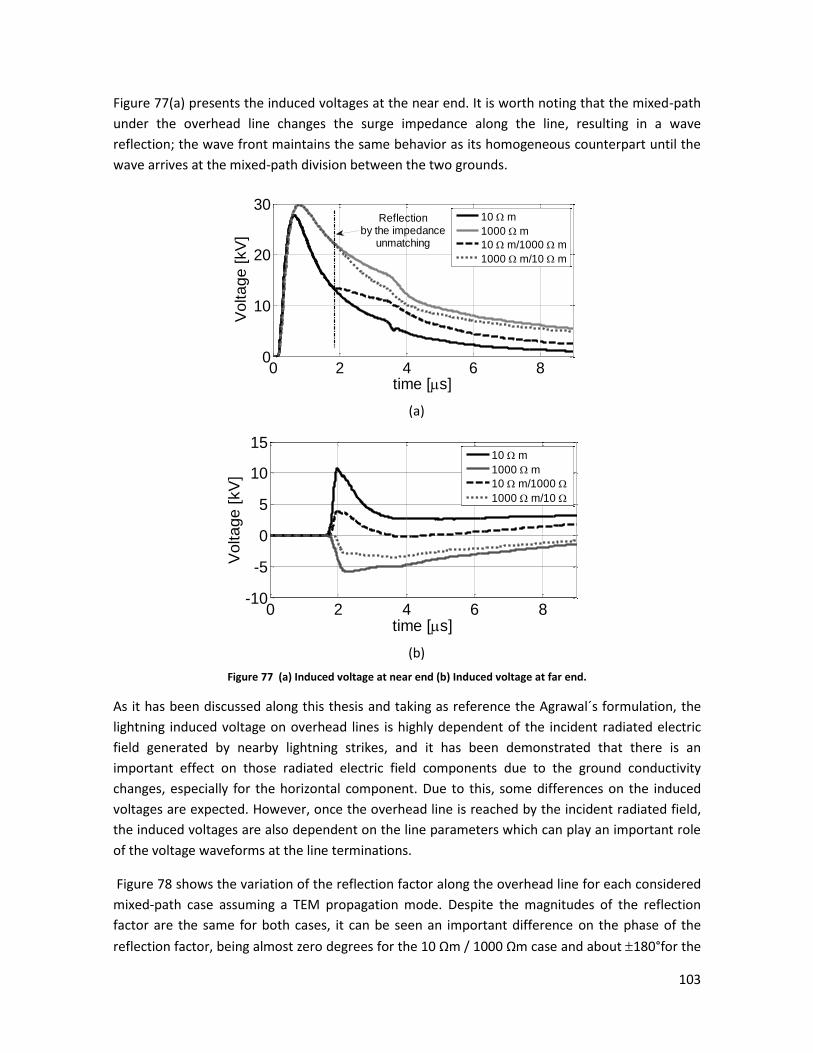
103
Figure 77(a) presents the induced voltages at the near end. It is worth noting that the mixed-path
under the overhead line changes the surge impedance along the line, resulting in a wave
reflection; the wave front maintains the same behavior as its homogeneous counterpart until the
wave arrives at the mixed-path division between the two grounds.
(a)
(b)
Figure 77 (a) Induced voltage at near end (b) Induced voltage at far end.
As it has been discussed along this thesis and taking as reference the Agrawal´s formulation, the
lightning induced voltage on overhead lines is highly dependent of the incident radiated electric
field generated by nearby lightning strikes, and it has been demonstrated that there is an
important effect on those radiated electric field components due to the ground conductivity
changes, especially for the horizontal component. Due to this, some differences on the induced
voltages are expected. However, once the overhead line is reached by the incident radiated field,
the induced voltages are also dependent on the line parameters which can play an important role
of the voltage waveforms at the line terminations.
Figure 78 shows the variation of the reflection factor along the overhead line for each considered
mixed-path case assuming a TEM propagation mode. Despite the magnitudes of the reflection
factor are the same for both cases, it can be seen an important difference on the phase of the
reflection factor, being almost zero degrees for the 10 Ωm / 1000 Ωm case and about 180°for the
0 2 4 6 80
10
20
30
time [s]
Vo
lta
ge
[kV
]
10 m
1000 m
10 m/1000 m
1000 m/10 m
Reflectionby the impedance
unmatching
0 2 4 6 8-10
-5
0
5
10
15
time [s]
Voltage [
kV
]
10 m
1000 m
10 m/1000
1000 m/10

104
1000 Ωm / 10 Ωm case; this means that the reflection for the latter case is negative at the division
between the two grounds. This situation reduces the voltage reflected at the near end of the line
once the reflected traveling wave reaches it (dotted line on Figure 77(a)). For the first case (10 Ωm
/ 1000 Ωm) the reflection factor results positive, increasing the voltage at the near end (black
dashed waveforms on Figure 77(a)).
a)
(b) Figure 78 (a) Reflection factor magnitude (b) Reflection factor phase.
As it is shown in Figure 77 (b) the far end induced voltages have been highly affected by the mixed
path condition when they are compared with the homogeneous case. Although their polarity
coincide with the polarities obtained for the homogeneous case, the magnitude of the induced
voltages is reduced to almost two to three times compared to those voltages obtained from the
homogeneous case. This effect can be understood by the horizontal electric field behavior
presented in Figure 76(a)). For case III, the lightning electromagnetic field initially travels above a
low resistivity ground; as this value changes on the second half of the line to a high resistivity
value, the contributions of the horizontal electric field coupled to the line tend to reduce the
induced voltage due to the negative polarity presented on them (Black waveforms on Figure
76(a)). For Case IV the same occurs, the horizontal electric field coupled to the line also tends to
reduce the induced voltage; in this case the induced voltage results in a lower magnitude due to
100
102
104
106
0.01
0.02
0.03
0.04
0.05
0.06
Frequency [Hz]
Re
fle
ctio
n F
acto
r M
ag
nitu
de
10 m / 1000 m
1000 m / 10 m
100
102
104
106
-200
-100
0
100
200
Frequency [Hz]
Reflection F
acto
r A
ngle
[deg]
10 m / 1000 m
1000 m / 10 m
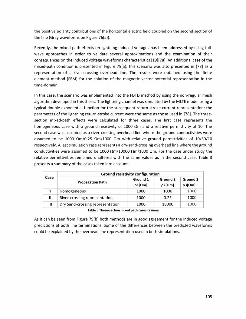
105
the positive polarity contributions of the horizontal electric field coupled on the second section of
the line (Gray waveforms on Figure 76(a)).
Recently, the mixed-path effects on lightning induced voltages has been addressed by using full-
wave approaches in order to validate several approximations and the examination of their
consequences on the induced voltage waveforms characteristics [19][78]. An additional case of the
mixed-path condition is presented in Figure 79(a), this scenario was also presented in [78] as a
representation of a river-crossing overhead line. The results were obtained using the finite
element method (FEM) for the solution of the magnetic vector potential representation in the
time-domain.
In this case, the scenario was implemented into the FDTD method by using the non-regular mesh
algorithm developed in this thesis. The lightning channel was simulated by the MLTE model using a
typical double-exponential function for the subsequent return-stroke current representation; the
parameters of the lightning return-stroke current were the same as those used in [78]. The three-
section mixed-path effects were calculated for three cases. The first case represents the
homogeneous case with a ground resistivity of 1000 Ωm and a relative permittivity of 10. The
second case was assumed as a river-crossing overhead line where the ground conductivities were
assumed to be 1000 Ωm/0.25 Ωm/1000 Ωm with relative ground permittivities of 10/30/10
respectively. A last simulation case represents a dry-sand-crossing overhead line where the ground
conductivities were assumed to be 1000 Ωm/10000 Ωm/1000 Ωm. For the case under study the
relative permittivities remained unaltered with the same values as in the second case. Table 3
presents a summary of the cases taken into account.
Case Ground resistivity configuration
Propagation Path Ground 1
ρ1*Ωm+
Ground 2
ρ2*Ωm+
Ground 3
ρ3*Ωm+
I Homogeneous 1000 1000 1000
II River-crossing representation 1000 0.25 1000
III Dry Sand-crossing representation 1000 10000 1000
Table 3 Three-section mixed path cases resume
As it can be seen from Figure 79(b) both methods are in good agreement for the induced voltage
predictions at both line terminations. Some of the differences between the predicted waveforms
could be explained by the overhead line representation used in both simulations.

106
ρ1, ε1, μ 1
Lightning ChannelMLTE Model
λ=2000V=0.43C
ρ2, ε2, μ2 ρ1, ε1, μ 1
200m
10m
1500m
50m 600m
200m
Overhead Line
NE FE
Overhead Line
Strike
Top View
(a)
(b)
Figure 79 (a) Relevant geometry of the simulation set-up (b) Comparison of the induced voltages by using the FEM method and the FDTD method (circles: FEM, solid: FDTD)
The results presented in Figure 79(b) are compared with the homogeneous case and the
comparison is presented in Figure 80 for the near and far end. The results at the near end are in
agreement with the analysis presented before for the two-section mixed path; As in the two-
section mixed path the reflected wave from the first impedance change in the case II (1000
Ωm/0.25 Ωm/1000 Ωm) leads to a decrease of the near end induced voltage (dashed line in Figure
80(a)). However, the increasing of the ground conductivity due to the second mixed-path affects
representatively the far end induced voltage. This behavior can be related with the behavior of the
horizontal electric field component as in the simulation set-up presented before. As it was
presented in section 6.3.1, there is a “recovery effect” (there is no a bipolar waveform above the
high conductivity section) of the horizontal electric field component when traveling from a high
resistivity soil to a low resistivity one, increasing the contribution of this component on the
electromagnetic coupling with the overhead line and leading to a higher induced voltage at the far
0 2 4 6 80
100
200
time [s]
Induced V
oltage [
kV
]
Mixed FEM
Mixed FDTD
NE
FE

107
end. In the other hand, the third case represents a positive reflection coefficient at the first mixed
path section leading to a higher voltage at the near end, being again in agreement with the results
presented for the two-section mixed-path analysis (dotted line in Figure 80(a)). As the middle
section presents a higher resistivity ground value, the horizontal electric field component
decreases its contribution on the induced voltages at the far end due to the change of polarity
evidenced in section 6.3.1.
(a)
(b)
Figure 80 Induced Voltages for a Three-section mixed-path (a) Near End (b) Far End
As it has been presented in this section, the mixed propagation path for the lightning radiated
fields, could lead to a variation of the induced voltage waveforms and magnitudes when compared
with the homogeneous lossy ground case. The effects that have been evidenced are multi-variable
dependent and the total result is obtained by several contributions, however two main features
can be derived from the induced voltage characteristics in presence of a mixed-path: First, the
calculation of the surge impedance of the overhead line can be useful for a qualitative description
of the reflected waves at the division of the mixed-paths and their contribution to the induced
voltages at the line terminations and second, the effects of the mixed-path on the components of
0 2 4 6 80
50
100
150
Indu
ce
d V
olta
ge
[kV
]
time [s]
Homogeneous
1km/0.25m/1km
1km/10km/1km
0 2 4 6 8-50
0
50
100
Indu
ce
d V
olta
ge
[kV
]
time [s]
Homogeneous
1km/0.25m/1km
1km/10km/1km

108
the lightning radiated electric fields lead to strong variations on the induced voltages due to the
electromagnetic coupling with the overhead line.
7.1.3 Non-Uniform Ground Effect
This section presents some results of lightning induced voltages due to a typical subsequent return
stroke current waveform where different ground irregularities are present. The non-uniform
ground effect on the induced voltages was taken into account by means of the full-wave solution
based on the FDTD method and using the non-regular meshing method developed in this thesis
and discussed in detail in section 3.8.
The first simulation case corresponds to a lightning striking at the top of a step mountain which
induces an overvoltage on a single overhead line located at the bottom of it; Figure 81(a) depicts
the geometry for the case under study. The lightning return stroke current was simulated by
means of a MTLE model with velocity of propagation of 0.3 times the speed of light and a constant
decay λ=1700. The overhead line is 1km in length and 10m in height, and was represented as a
thin-wire with 1cm in radius by using the INY model presented in section 3.7.4. The line has been
terminated with a 330Ω resistor at each end. The ground resistivity was assumed to be 1000Ωm
and a relative permittivity of 10ε0.
Similar situations have been analyzed in literature when the lightning strikes to nearby conductive
tall objects and tall structures, and the effects on the induced voltages are related with the
multiple reflections of the current occurring between the top of the structure and the ground [25].
In this scenario no current reflections are considered along the channel, only the effects on the
induced voltages due to the radiated fields caused by the ground geometry are taken into account.
NE
10
m
Overhead line
ρ1, μ1, ε1
330Ω
1000 m
Ground 1
FE
50 m
50 m
(a)
Lightning
Channel
10
m
Overhead line
ρ1, μ1, ε1
Ground50m 1000m
50
m
330Ω 330Ω
(b)
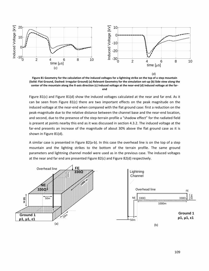
109
(c)
(d)
Figure 81 Geometry for the calculation of the induced voltages for a lightning strike on the top of a step mountain (Solid: Flat Ground, Dashed: Irregular Ground) (a) Relevant Geometry for the simulation set-up (b) Side view along the
center of the mountain along the X-axis direction (c) Induced voltage at the near-end (d) induced voltage at the far-end
Figure 81(c) and Figure 81(d) show the induced voltages calculated at the near and far end. As it
can be seen from Figure 81(c) there are two important effects on the peak magnitude on the
induced voltage at the near-end when compared with the flat ground case: first a reduction on the
peak-magnitude due to the relative distance between the channel base and the near-end location,
and second, due to the presence of the step-terrain profile a “shadow effect” for the radiated field
is present at points nearby this end as it was discussed in section 4.3.2. The induced voltage at the
far-end presents an increase of the magnitude of about 30% above the flat ground case as it is
shown in Figure 81(d).
A similar case is presented in Figure 82(a-b). In this case the overhead line is on the top of a step
mountain and the lighting strikes to the bottom of the terrain profile. The same ground
parameters and lightning channel model were used as in the previous case. The induced voltages
at the near and far end are presented Figure 82(c) and Figure 82(d) respectively.
10
m
Overhead line330Ω
1000 m
FE
NE
ρ1, μ1, ε1Ground 1
50
m
330Ω
50m
50m
(a)
Lightning
Channel
10
mOverhead line
ρ1, μ1, ε1
Ground 1
1000m
330Ω 330Ω
50m
NE
FE
(b)
0 2 4 6 8 10-10
0
10
20
Induced V
oltage [
kV
]
time [s]0 2 4 6 8 10
-30
-20
-10
0
10
Ind
uce
d V
olta
ge
[kV
]
time [s]
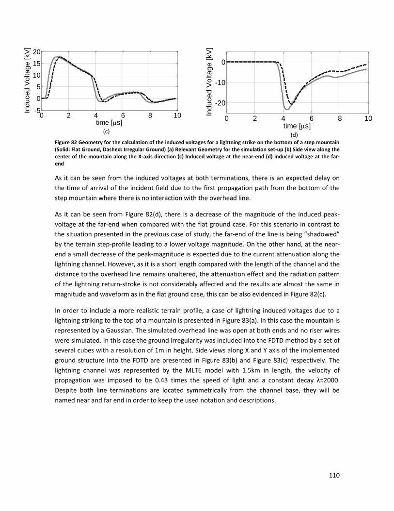
110
(c)
(d) Figure 82 Geometry for the calculation of the induced voltages for a lightning strike on the bottom of a step mountain (Solid: Flat Ground, Dashed: Irregular Ground) (a) Relevant Geometry for the simulation set-up (b) Side view along the center of the mountain along the X-axis direction (c) Induced voltage at the near-end (d) induced voltage at the far-end
As it can be seen from the induced voltages at both terminations, there is an expected delay on
the time of arrival of the incident field due to the first propagation path from the bottom of the
step mountain where there is no interaction with the overhead line.
As it can be seen from Figure 82(d), there is a decrease of the magnitude of the induced peak-
voltage at the far-end when compared with the flat ground case. For this scenario in contrast to
the situation presented in the previous case of study, the far-end of the line is being “shadowed”
by the terrain step-profile leading to a lower voltage magnitude. On the other hand, at the near-
end a small decrease of the peak-magnitude is expected due to the current attenuation along the
lightning channel. However, as it is a short length compared with the length of the channel and the
distance to the overhead line remains unaltered, the attenuation effect and the radiation pattern
of the lightning return-stroke is not considerably affected and the results are almost the same in
magnitude and waveform as in the flat ground case, this can be also evidenced in Figure 82(c).
In order to include a more realistic terrain profile, a case of lightning induced voltages due to a
lightning striking to the top of a mountain is presented in Figure 83(a). In this case the mountain is
represented by a Gaussian. The simulated overhead line was open at both ends and no riser wires
were simulated. In this case the ground irregularity was included into the FDTD method by a set of
several cubes with a resolution of 1m in height. Side views along X and Y axis of the implemented
ground structure into the FDTD are presented in Figure 83(b) and Figure 83(c) respectively. The
lightning channel was represented by the MLTE model with 1.5km in length, the velocity of
propagation was imposed to be 0.43 times the speed of light and a constant decay λ=2000.
Despite both line terminations are located symmetrically from the channel base, they will be
named near and far end in order to keep the used notation and descriptions.
0 2 4 6 8 10-5
0
5
10
15
20
Ind
uce
d V
olta
ge
[kV
]
time [s]0 2 4 6 8 10
-20
-10
0
Induced V
oltage [
kV
]
time [s]

111
500 m
500 m
10
mOverhead line
ρ1, μ1, ε1
1000 m
Ground 1 NE
FE
250 m
Gaussian Mountain
50 m
Lightning Channel
(a)
(b)
(c)
Figure 83 Geometry for the calculation of the induced voltages for a lightning strike on the top of a Gaussian Mountain (a) Relevant Geometry for the simulation set-up (b) Side view along the center of the mountain along the X-
axis direction (c) Side view along the center of the mountain along the Y-axis direction
Figure 84 presents the induced voltages at the near and far end of the line. Similar results were
presented in [28] by using a full-wave solution by means finite element method (FEM) for a
striking point to the top of a cone-shaped mountain with a similar height. The proposed scenario
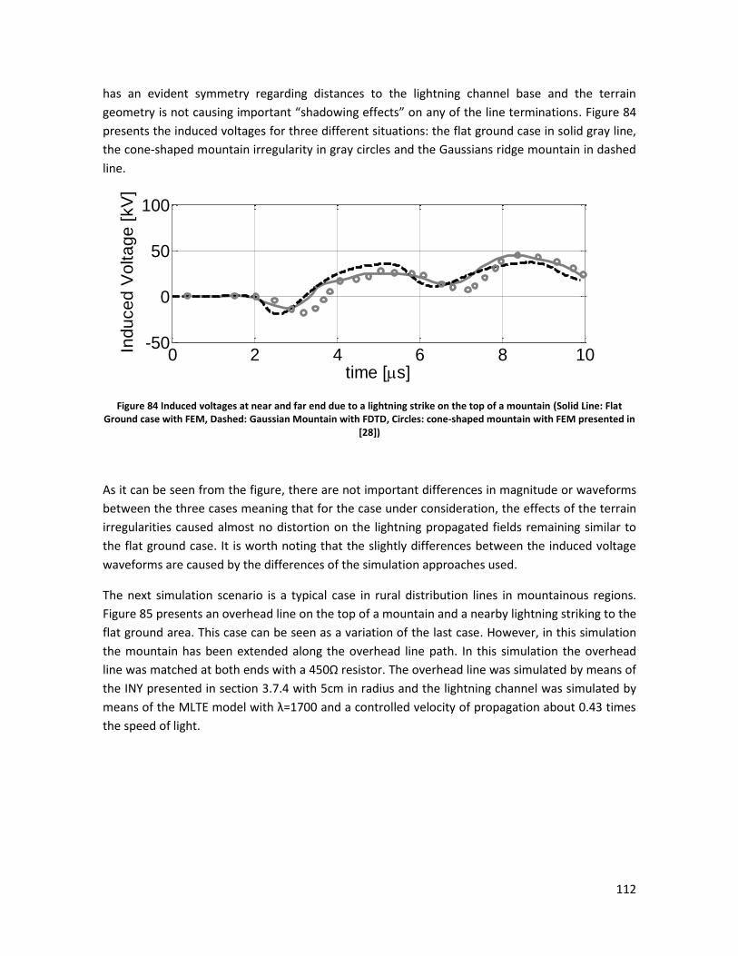
112
has an evident symmetry regarding distances to the lightning channel base and the terrain
geometry is not causing important “shadowing effects” on any of the line terminations. Figure 84
presents the induced voltages for three different situations: the flat ground case in solid gray line,
the cone-shaped mountain irregularity in gray circles and the Gaussians ridge mountain in dashed
line.
Figure 84 Induced voltages at near and far end due to a lightning strike on the top of a mountain (Solid Line: Flat Ground case with FEM, Dashed: Gaussian Mountain with FDTD, Circles: cone-shaped mountain with FEM presented in
[28])
As it can be seen from the figure, there are not important differences in magnitude or waveforms
between the three cases meaning that for the case under consideration, the effects of the terrain
irregularities caused almost no distortion on the lightning propagated fields remaining similar to
the flat ground case. It is worth noting that the slightly differences between the induced voltage
waveforms are caused by the differences of the simulation approaches used.
The next simulation scenario is a typical case in rural distribution lines in mountainous regions.
Figure 85 presents an overhead line on the top of a mountain and a nearby lightning striking to the
flat ground area. This case can be seen as a variation of the last case. However, in this simulation
the mountain has been extended along the overhead line path. In this simulation the overhead
line was matched at both ends with a 450Ω resistor. The overhead line was simulated by means of
the INY presented in section 3.7.4 with 5cm in radius and the lightning channel was simulated by
means of the MLTE model with λ=1700 and a controlled velocity of propagation about 0.43 times
the speed of light.
0 2 4 6 8 10-50
0
50
100
Indu
ce
d V
olta
ge
[kV
]
time [s]

113
Overhead line
ρ1, μ1, ε1
Ground 1
NE
FE
250 m
Gaussian Mountain
Lightning Channel
50 m
450Ω
500 m
500 m
1000 m
450Ω
10
m
Figure 85 Overhead Line on the top of a mountain
In this scenario the location of the overhead line respect to the lightning channel lead to an
increase of the induced voltage in almost 50% in its peak magnitude as is presented in Figure 86.
Figure 86 Induced Voltage for an Overhead Line on the top of a mountain (Solid Line: Flat Ground Case, Dashed: non-uniform ground)
It is worth noting that the induced voltage for the irregular terrain case presented in Figure 86
coincides for the first part of the waveform (about 3.4µs) with the flat ground case. In order to
validate these effects of the previous scenario on the lightning radiated fields, a variation of the
case presented before is depicted in Figure 87(a). In this scenario the overhead line is at the same
ground level as the channel base and the mountain is located 200m behind the overhead line. The
same ground parameters and lightning channel model as in the previous case was used.
0 2 4 6 8 10-10
0
10
20
Ind
uce
d V
olta
ge
[kV
]
time [s]

114
10
m
Overhead line
ρ1, μ1, ε1Ground 1
NE
FE
Gaussian Mountain
Lightning Channel
450Ω
500 m
500 m
200 m
50 m450Ω
50 m
(a)
(b)
Figure 87 Induced Voltage for an Overhead Line with a mountain behind it (a) Relevant Geometry (b) Induced Voltage for an Overhead Line with a mountain behind (Solid Line: Flat Ground Case, Dashed: non-uniform ground)
Figure 87(b) presents the results of the induced voltage for the case under consideration. It can be
seen that the difference between the irregular terrain case and the flat ground case begins once
the reflected wave arrives from the mountain (at about 2.4µs). The effect of the reflect wave from
the mountain behind the line represents less than the 3% in peak magnitude when compared with
the flat ground but there can be observed differences of about 10% in some parts of the waveform
due to the increase of the incident field at the overhead line location.
The next simulation cases are focused on the scenarios where the irregular terrain is under the
overhead line. For these simulation scenarios the line parameters are highly affected by the
irregular terrain and the interaction between the overhead line and the incident lightning
electromagnetic field cannot be analyzed by using the uniform transmission line theory.
0 2 4 6 8 10
0
10
20
30
Indu
ce
d V
olta
ge
[kV
]
time [s]
Effect of the reflected wavefrom the mountain

115
A typical case of an overhead line above non-uniform ground is presented in Figure 88, for this
case the ends of the overhead line are located between two mountains. The same simulation
parameters for the lightning channel and overhead line are used. The ground resistivity value
remained unaltered in 1000Ωm. Near and far end names will be also used for referring the line
terminations in the current case although they are at the same distance from the lightning channel
base.
Overhead line
ρ1, μ1, ε1
Ground 1
NE
FE
250 m
Gaussian Mountain
Lightning Channel
450Ω
50 m
500 m
500 m
1000 m1
0 m
450Ω
Lightning
Channel
10
m
Overhead line
ρ1, μ1, ε1Ground 1
50
m
1000m
500m Figure 88 Overhead Line on between the top of two mountains (a) Relevant Geometry of the scenario (b) Side View
The comparison of the induced voltages between the non-uniform case and the flat ground case
are presented in Figure 89. As it can be seen from the induced voltage for the irregular terrain
scenario, the effect of the lightning electromagnetic fields and its interaction with the overhead
line lead to almost three times the peak voltage magnitude for the homogeneous case.
Figure 89 Induced Voltage for an Overhead Line between the tops of two mountains (Solid Line: Flat Ground Case, Dashed: non-uniform ground)
As it has been discussed along this thesis, the lightning induced voltage problem involves several
parameters and variables that must be taken into account for the calculations, not only the effects
0 2 4 6 8 10-20
0
20
40
60
Ind
uce
d V
olta
ge
[kV
]
time [s]

116
of the propagation path on the lightning radiated fields, but also the overhead line characteristics.
The case under study presents both effects at the same simulation scenario. In order to address
the line-parameters modifications due to the ground non-uniformity beneath the overhead line, a
comparison of the calculated characteristic impedance for a single-wire overhead line for different
heights is presented in Figure 90. These results show that under the TEM approach, the surge
impedance increases with the relative height of the conductor to the ground level for a wide
frequency band, therefore the propagating wave along the overhead line will face several
reflections.
Figure 90 Characteristic impedance of a single-wire overhead line above 1000Ωm lossy ground depending on the conductor height by using the TEM approach
Based on the results presented in Figure 90 the increase of the induced voltage in Figure 89 is the
result of a contribution of both effects: the propagation path effects and their electromagnetic
coupling with the overhead line, and the line-parameter modifications which can lead to an
increase of the induced voltage at both ends.
The next case of study quantifies the lightning induced over-voltages for a more realistic case of
irregular terrains beneath the overhead line. For this case a cliff is present under the line as it is
shown in Figure 91(a-b). In some practical situations there is not possibility for planting poles on
the cliff bottom and two robust towers must be installed at each extreme of the cliff leading to a
non-uniform line configuration. The lightning channel was simulated by means of a MTLE model
with a velocity of propagation about 0.5 times the speed of light and a constant decay λ=1700. The
simulation was performed assuming a ground resistivity of ρ1=1000Ωm and permittivity εr1=10.
The overhead line is terminated with 330Ω resistors at both ends and the wire risers are also
included at the line terminations. Despite both line terminations are located symmetrically from
the channel base, they will be named near and far end for maintaining the used notation and
descriptions.
100
102
104
106
108
300
400
500
600
Frequency [Hz]
Zc [
]
10m20m 30m
50m40m

117
50 m
500 m
500 m
10
m
Lightning
Channel
Overhead line
ρ1, μ1, ε1
330Ω
1000 m
Ground 1
NE
FE
330Ω
(a)
Lightning
Channel
10
m
50
m
Overhead line
ρ1, μ1, ε1 Ground
1300m 100m100m 500m
330Ω 330Ω NE FE
(b)
(c)
Figure 91 (a) Description of the Simulation Set-up for the irregular ground effects on induced voltages (b) Side View of the simulation set-up (c) Induced Voltage Comparison when a cliff is present under the ground
Figure 91(c) presents the comparison between the induced voltages on the near and the far end
when a cliff is present under the overhead line compared with the flat ground induced voltage
situation. As it can be seen, the presence of the cliff under the overhead line increases
considerably the peak-value and the waveform at each ends of the line, reaching to almost 5 times
the magnitude of the flat ground case.
It is worth noting that the induced voltages are not symmetric as in the flat ground case due to the
location of the cliff section. This leads to a higher induced voltage at the near-end when compared
with the induced voltage at the far-end. This result evidences the markedly effect that has the
propagation path on the lighting radiated fields and the line-parameters modification for the
induced voltage calculations.
An additional simulation based on the last case of study was performed in order to represent a
river-crossing overhead line between two mountains. Figure 92(a) presents a combination
between a cliff and a conductive change at its bottom which can be also seen a mixed-path
condition for the propagating field. The simulation was performed assuming a ground resistivity of
0 2 4 6 8 10
0
50
100
Induced V
oltage [
kV
]
time [s]
NE
FECliff Profile
Flat Ground
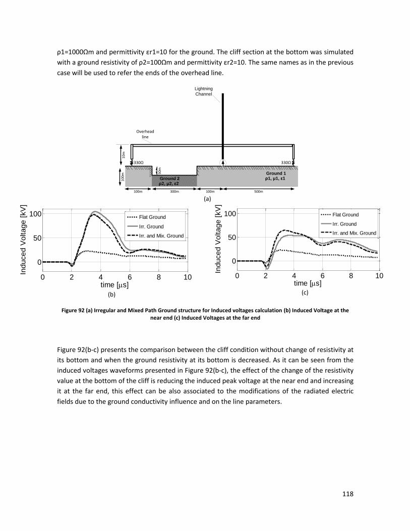
118
ρ1=1000Ωm and permittivity εr1=10 for the ground. The cliff section at the bottom was simulated
with a ground resistivity of ρ2=100Ωm and permittivity εr2=10. The same names as in the previous
case will be used to refer the ends of the overhead line.
Lightning
Channel
10
m
50
m
Overhead line
ρ1, μ1, ε1Ground 1
300m
10
0m
100m 500m
ρ2, μ2, ε2Ground 2
100m
330Ω 330Ω
(a)
(b)
(c)
Figure 92 (a) Irregular and Mixed Path Ground structure for Induced voltages calculation (b) Induced Voltage at the near end (c) Induced Voltages at the far end
Figure 92(b-c) presents the comparison between the cliff condition without change of resistivity at
its bottom and when the ground resistivity at its bottom is decreased. As it can be seen from the
induced voltages waveforms presented in Figure 92(b-c), the effect of the change of the resistivity
value at the bottom of the cliff is reducing the induced peak voltage at the near end and increasing
it at the far end, this effect can be also associated to the modifications of the radiated electric
fields due to the ground conductivity influence and on the line parameters.
0 2 4 6 8 10
0
50
100
Ind
uce
d V
olta
ge
[kV
]
time [s]
Flat Ground
Irr. Ground
Irr. and Mix. Ground
0 2 4 6 8 10
0
50
100In
duced V
oltage [
kV
]
time [s]
Flat Ground
Irr. Ground
Irr. and Mix. Ground

119
8 Conclusions Remarks and Future work
This thesis dealt with all of the three aspects of the lightning induced voltage problem: return
stroke models, calculation of lightning radiated fields and the evaluation of the induced voltages
on single-phase overhead lines.
Several methods used nowadays for evaluating lighting radiated fields were analyzed in this thesis
showing their theoretical basis and specifying their limitations, especially for calculations within
the near field region.
A full wave solution was implemented using the FDTD Method including a non-regular mesh in
order to represent different geometric features and allowing adequate near-field interactions
calculation. The implemented FDTD scheme based on a non-regular meshing algorithm, allowed
the representation of the ground irregularities and the overhead lines with a finer mesh and a
coarser domain was used the rest of the problem space. An experimental case of a typical cross-
talk problem was analyzed using the classical implementation of the FDTD and the non-regular
mesh approach, showing its advantages over the classical formulation in representing larger
problem space dimensions and lesser number of Yee’s cells.
By means of the proposed methodology for representing the problem space by means a non-
regular mesh, the calculation of lightning induced voltages became available including complex
geometry into the simulation scenario in order to achieve more realistic representations of actual
situations.
The effects on the lightning radiated fields due to the presence of different propagation paths
were analyzed along this thesis showing their representative influence especially for the horizontal
electric field. Several approaches based on far-field formulation and cylindrical symmetry
regarding geometry were analyzed and compared with the full-wave solution by using the FDTD
method, showing that those approaches could lead for some of the cases to an over or under
estimation in the calculations of the radiated field components.
The mixed propagation path for the lightning radiated fields, lead to a variation of the induced
voltage waveforms and magnitudes when compared with the homogeneous lossy ground case.
The effects that have been evidenced are multi-variable dependent and the total result is obtained
by several contributions. However, two main features can be derived from the induced voltage
characteristics in presence of a mixed-path: First, the calculation of the characteristic impedance
of the overhead line can be useful for a qualitative description of the reflected waves at the
division of the mixed-paths and their contribution to the induced voltages at the line terminations
and second, the effects of the mixed-path on the components of the lightning radiated electric
fields lead to strong variations on the induced voltages due to the electromagnetic coupling with
the overhead line.

120
Regarding irregular grounds, relatively important effects on the induced voltages were obtained
when an effect of “shadowing” is present for some segments of the overhead line and the
irregularities are larger enough to diffract part of the radiated fields. However, the most
representative variations were obtained when the irregular terrain is below the overhead line
leading to over-voltages near 5 times higher than those occurring over flat ground scenarios.
Based on the obtained results and the analysis made along this thesis, it is proposed as a future
work to perform experimental testing for induced voltages above inhomogeneous and irregular
grounds in reduced scale experimentations and full-scale controlled induced voltages by triggered
lightning experiments, in order to validate their theoretical effects.
From the theoretical analysis and by using the implemented FDTD scheme, it will be interesting to
address the modeling of the return-stroke including inclination and tortuosity in order to quantify
their effects on the induced voltages taking into account irregular and inhomogeneous
propagation paths in order to simulate a more realistic scenario.

121
9 References
[1] M. Master and M. Uman, “Lightning Induced Voltages on Power Lines: Theory”, IEEE Transaction on Power apparatus and Systems, Vol. PAS-103, No. 9, Semptember 1984.
[2] A.K. Agrawal, H. J. Price and H.H. Gurbaxani, “Transient response of multiconductor transmission lines excited by a nonuniform electromagnetic field”, IEEE Transactions on , vol.22, no.2, pp.119-129, May 1980.
[3] A.J. Eriksson, M.F. Stringfellow and D.V. Meal, “Lightning induced over-voltages on overhead distribution lines”, IEEE Transaction on Power apparatus and Systems, Vol. PAS-101, pp. 960-969, April 1982.
[4] M. Master, M. Uman, W. Beasley, and M. Darveniza, “Lightning Induced Voltages on Power Lines: Experiment”, IEEE Transaction on Power apparatus and Systems, Vol. PAS-103, No. 9, Semptember 1984.
[5] V. Rakov and M. Uman, “Lightning Physics and Effects”, 2003, Ed. Cambridge University Press.
[6] Rachidi, F., “Recent Progress in Lightning Return Stroke Modeling and Eletromagnetic Field Computation”, International Symposium on Lightning Protection SIPDA XI, Brazil 2011.
[7] Y. Baba, and V.A. Rakov, “Electromagnetic models of the lightning return stroke” Journal of Geophysical Research, vol. 112, Feb. 2007.
[8] Y. Baba and V. Rakov, “Applications of the Electromagnetic Models on the Lightning Return Stroke”, IEEE Trans, on Power Delivery, Vol.23 No.2, April 2008.
[9] C.A. Nucci, “Lightning Induced Voltages on Overhead Power Lines”, Part I, II and III, Electra, August 1995.
[10] J. Herrera, E., Pérez, and H.,Torres, “Statistical Evaluation of Transferred Voltages Through Transformers Due to Lightning Induced Overvoltages”, IEEE Bologna PowerTech Conference, June 2003.
[11] E. Perez, J. Herrera and H., Torres, “Sensitivity Analysis on Induced Voltages on Distribution Lines”, IEEE Bologna PowerTech Conference, June 2003.
[12] A., Borghetti, A. Morched, F. Napolitano, F., Nucci, C.A. and Paolone, M., “Lightning-Induced Overvoltages Transferred through Distribution Power Transformers”, IEEE Transaction on Power Delivery, Vol. 24, No.1, January 2009.
[13] IEEE Guide for Improving the Lightning Performance of Electric Power Overhead Distribution Lines, IEEE Std 1410-2010 (Revision of IEEE Std 1410-2004).
[14] E. Sunde, “Earth Conduction effects in Transmission Systems”, Dover Publications, 1949.
[15] F. Rachidi , C. A. Nucci , M. Ianoz and C. Mazzetti "Influence of a lossy ground on lightning-induced voltages on overhead lines", IEEE Trans. Electromagn. Compat., vol. 38, no. 3, pp.250 -264 1996.
[16] T.S.M.Maclean and Z. Wu, “Radion Wave Propagation Over Ground”, 1993, Chapman&Hall.
[17] V. Cooray, “On the Accuracy of Several Approximate Theories Used in Quantifying the propagation Effects on Lightning Generated Electromagnetic Fields”, IEEE Transactions on Antennas and Propagation, Vol 56, No.7, July 2008.
[18] J. R. Wait, “The Ancient and Modern History of EM Ground-Wave Propagation”, IEEE Antennas and Propagation Magazine, Vol. 40, No.5, October 1998.
[19] A. Shoory, A. Mimouni, F. Rachidi, V. Cooray, and M. Rubinstein, “On the accuracy of approximate techniques for the evaluation of lightning electromagnetic fields along a mixed propagation path,” Radio Science, vol. 46, no. 2, p. n/a–n/a, 2011.
[20] V. Cooray,”Horizontal Electric Field Above-and Underground Produced by Lightning Flashes”, IEEE Transactions on Electromagnetic Compatibility, vol. 52, no. 4, pp. 936 – 943, Nov. 2010.
[21] M. Rubinstein "An approximation formula for calculation of the horizontal electric field from lightning at close, intermediate, and long ranges", IEEE Trans. Electromagn. Compat., vol. 38, no. 3, pp.531 -535 1996.
[22] V. Cooray, “Some considerations on the “Cooray-Rubistein” Formulation used in deriving the horizontal Electric field of lightning Return Strokes over Finitely Conducting Ground”, IEEE Transactions on Electromagnetic Compatibility, Vol 44, No.4, November 2002.
[23] M. Ishii, K. Michishita and Y. Hongo, “Experimental Study of Lightning-Induced Voltage on an Overhead Wire over Lossy Ground” IEEE Transactions on Electromagnetic Compatibility, vol. 41, no. 1, pp. 39 – 45, Feb. 1999.
[24] Y. Baba and V. A. Rakov, “Voltages Induced on an Overhead Wire by Lightning Strikes to a Nearby Tall Grounded Object” IEEE Transactions on Electromagnetic Compatibility, vol. 48, no. 1, pp. 212 – 224, Feb. 2006.
[25] D. Pavanello, “Electromagnetic Radiation from Lightning Return Strokes to Tall Structures”, PhD Dissertation Thesis, École polytechnique fédérale de Lausanne, 2007.
[26] A. Piantini and J.M. Janiszewski, “Lightning-Induced Voltages on Overhead Lines- Aplication of the Extended Rusck Model”, IEEE Trans. Electromagn. Compatibility, Vol 51, No.3, November, 2009.
[27] E. Soto, E.Perez and J. Herrera, “Electromagnetic Field Due to Lightning Striking on Top of a Cone-Shaped Mountain using the FDTD”, IEEE Trans. Electromagn. Compatibility, February 2014.
[28] J. Paknahad, K. Sheshyekani, M. Hamzeh and F. Rachidi, “Lightining Electromagnetic Fields and their Induced Voltages on Overhead Lines: The eefect of a non-flat Lossy Ground”, 2014 International Conference on Lightning Protection (ICLP), vol., no., pp.286,289, 7-11 Oct. 2014.
[29] K. Yee, “Numerical solution of initial boundary value problems involving maxwell’s equations in isotropic media,” IEEE Transactions on Antennas and Propagation, vol. 14, no. 3, pp. 302 –307, May 1966.
[30] A. Taflove, and S. Hagness, "Computational Electrodynamics: The Finite-Difference Time-Domain Method", Artech House, 2005.

122
[31] A.Z. Elshebereni, V. Demir, “The finite Difference Time Domain Method for Electromagnetics With MATLAB Simulations”. Raleigh, NC: SciTech Pub., 2009.
[32] K. Kunz and R. Luebbers, “The Finnite difference Time Domain Method for Electromagnetics” CRC Press, 1993.
[33] G. Mur, “Absorbing Boundary Conditions for the Finite-Difference Approximation of the Time-Domain Electromagnetic-Field Equations”, IEEE Transactions on Electromagnetic Compatibility, vol. EMC-23, no. 4, pp. 377 – 382, Nov. 1981.
[34] B. Engquist, and A. Majda, “Absorbing Boundary Conditions for the numerical simulation of waves”, Mathematics of Computation, Vol.31,pp. 629-651, 1977.
[35] Z.P. Liao, H.L Wong, B.P. Yang and Y.F. Yuan, “A transmiting boundary for transient wave analyses”, Scientia Sinica (Series A), Vol XXVII, pp. 1063-1076, 1984.
[36] J.P . Berenger, “Perfectly matched layer for the Absorption of electromagnetic waves”, J. Computational Physics, Vol.114, pp.185-200, 1994.
[37] J.P . Berenger, “Perfectly matched layer for the FDTD solution of wave-interaction problems”, IEEE Trans. Antennas and Propagation, Vol. 44, pp.110-117, 1996.
[38] J.P . Berenger, “Three-dimensional perfectly matched layer for the absortion of electromagnetic waves”, J. Computational Physics, Vol.127, pp.363-379, 1996.
[39] J. Roden and S. Gedeney, “Convolution PML (CPML): An Efficient FDTD implmentation of the CFS-PML for arbitrary media”, Microwave Opt. Technol. Letters. Vol 27, no. 5 pp 334-339, 2000.
[40] K. Umashankar, A. Taflove, and B. Beker, “Calculation and experimental validation of induced currents on coupled wires in an arbitrary shaped cavity,” IEEE Transactions on Antennas and Propagation, vol. 35, no. 11, pp. 1248 – 1257, Nov. 1987.
[41] T. Noda and S. Yokoyama, “Thin wire representation in finite difference time domain surge simulation,” IEEE Transactions on Power Delivery, vol. 17, no. 3, pp. 840 – 847, Jul. 2002.
[42] Y. Taniguchi, Y. Baba, N. Nagaoka, and A. Ametani, "An Improved Thin Wire Representation for FDTD Computations", IEEE Transactions On Antennas And Propagation, Vol. 56, No. 10, October 2008.
[43] H. W. Dommel, Electromagnetic Transients Program (EMTP) Theory Book, Bonneville Power Administration, Portland, OR, 1986
[44] SINTEF Energy Research, ATPDRAW Version 3.5 Users’ Manual, Trondheim, Norway, 2002. Available on: http://www.eeug.org/files/secret/ATPDraw
[45] CanAm EMTP User Group, Alternative Transient Program (ATP) Rule Book, Portland, OR, 2001.
[46] C.R. Paul, “Analysis of Multiconductor Transmission Lines”, 2nd Edition, IEEE Press, John Wiley and Sons, 2007.
[47] C.R. Paul, “Introduction to Electromagnetic Compatibility”, 2nd Edition, Jhon Wiley & Sons, 2006.
[48] N. Theethayi and R. Thottappillil, Surge propagation and crosstalk in multiconductor transmission lines above ground, Electromagnetic Field Interaction with Transmission Linesfrom classical theory to HF radiation effects, Ed. By F. Rachidi and S. Tkachenko, WIT Press 2008.
[49] C. Balanis, Advanced Engineering Electromagnetics, Second Edition, John Wiley and Sons, 2012
[50] R.J. King, “Electromagnetic wave propagation over a constant impedance plane”, Radio Sciences, Vol 4, pp. 255-268,1969.
[51] R.J. King and G.A. Schlak, “The Ground Wave attenuation function for Propagation over highly Inductive Surface”, Scientific Report No. 37, Air Force Cambridge Research Laboratories, Office of Aerospace Research, August 1966.
[52] Ott, R.H. “A new method for predicting HF ground wave attenuation over inhomogeneous, irregular terrain”. Office of Telecommunications Boulder Co. Inst For Telecommunication Sciences, 1971.
[53] C. Constantinou, “Numerically intensive Propagation Prediction Methods”, Propagation of Radiowaves, Chp.21, Ed.Les Barclay, The Intitution for Engineering and Techology, 2012.
[54] Ott, R.H., “An alternative Integral Equation for Propagation over Irregular Terrain” Radio Science, vol. 6, Number 4, pp. 429–435, April 1971.
[55] J. R. Wait, Electromagnetic Waves in Stratified media, New York, Pergamon Press, Second Edition.
[56] R. J. King, S.W. Maley and J.R. Wait, “Groundwave propagation along three-section mixed paths”, Proc. IEE, Vol 113, No.5, May 1966.
[57] V. Cooray and K. Cummings, “Propagation effects caused by multi-section mixed paths on electric fields of lightning return strokes”. International Symposium on Lightning Protection. - Curitiba, Brazil. 2009.
[58] Q. Zhang; D. Li; Y. Zhang; J. Gao; Z. Wang, "On the Accuracy of Wait's Formula Along a Mixed Propagation Path Within 1 km from the Lightning Channel," Electromagnetic Compatibility, IEEE Transactions on , vol.54, no.5, pp.1042,1047, Oct. 2012.
[59] Y. Baba and V. A. Rakov, “On the mechanism of attenuation of current waves propagating along a vertical perfectly conducting wire above ground: application to lightning,” IEEE Transactions on Electromagnetic Compatibility, vol. 47, no. 3, pp. 521 – 532, Aug. 2005.
[60] S. Bonydi-Ram, R. Moini, S.H. H. Sagedghi and V.A. Rakov, “On the representation of lighthning return stroke as a lossy monopole antenna with inductive loading”, IEEE Transactions on Electromagnetic Compatibility, vol. 50, no. 1, pp. 118 – 127, Feb. 2008.
[61] V. Rakov and M.A. Uman, “Review and evaluation of lightning return stroke models including some aspects of their application”, IEEE Trans. Electromagnetic Compatibility, Vol.40 No.4, pp 403-426, Nov 1998.
[62] F. Rachidi and C.A. Nucci, “On the Master, Uman, Lin, Standler and the modified trasmission line lightning return stroke current models”, J. Geophys. Res, Vol.95, 1990.
[63] G. Maslowski and V. Rakov, “Equivalency of Lightning Return-stroke models employing lumped and distributed current sources”, IEEE Transactions on Electromagnetic Compatibility, vol. 49, no. 1, pp. 123 – 132, Feb. 2007.

123
[64] R. Moini , B. Kordi , G. Z. Rafi and V. A. Rakov "A new lightning return stroke model based on antenna theory", J. Geophys. Res., vol. 105, no. D24, pp.29693 -29702 2000.
[65] S. Bonydi-Ram, R. Moini, S.H. H. Sagedghi and V.A. Rakov, “On the representation of lighthning return stroke as a lossy monopole antenna with inductive loading”, IEEE Transactions on Electromagnetic Compatibility, vol. 50, no. 1, pp. 118 – 127, Feb. 2008.
[66] Gibson, W., The Method of Moments in Electromagnetics, 1st ed., vol. 1. Chapman & Hall, 2008.
[67] Burke, G. Numerical Electromagnetic Code NEC-4, Method of Moments, Part I, User´s Manual, Jan 1992.
[68] Q. Zhang, D. Li, Y. Fan, Y. Zhang, and J. Gao, “Examination of the Cooray-Rubinstein (C-R) formula for a mixed propagation path by using FDTD”, J. Geophys. Res., 2012.
[69] J. R. Wait "Concerning the horizontal electric field of lightning", IEEE Trans. Electromagn. Compat., vol. 39, no. 2, pp.186 1997.
[70] M. Khosravi-Farsani; R. Moini; S.H.H. Sadeghi; F., Rachidi, "On the Validity of Approximate Formulas for the Evaluation of the Lightning Electromagnetic Fields in the Presence of a Lossy Ground," Electromagnetic Compatibility, IEEE Transactions on , vol.55, no.2, pp.362-370, April 2013.
[71] V. Cooray, “Calculating Lightning-Induced Overvoltages in Power Lines: A Comparison of two Coupling Models”, IEEE Trans. Electromgan. Compatibility, Vol.36, No.3, August 1994.
[72] F. Rachidi, "Formulation of the field-to-transmission line coupling equations in terms of magnetic excitation field", IEEE Trans. Electromagn. Compat., vol. 35, no. 3, pp.404 -407 1993.
[73] V. Cooray and V. Sckuka, “Lightning-Induced Voltages in Power Lines: Validity of various Approximations made in Overvoltage Calculations”, IEEE Trans. Electromagn. Compatibility, Vol 40, No4, November, 1998.
[74] R.K. Pokharel, M. Ishii and Y. Baba, "Numerical Electromagnetic Analysis of Lightning-Induced Voltage Over Ground of Finite Conductivity", IEEE Transactions on Electromagnetic Compatibility, vol. 45, no. 4, pp. 651 – 656, Nov. 2003.
[75] C.A. Nucci, F. Rachidi, M. Ianoz and C. Mazzetti, “Lightning-Induced Voltages on Overhead Lines”, IEEE Trans. Electromagn. Compatibility, Vol.35, No.1, Febraury 1993.
[76] B. Yang, B.H. Zhou, C. Gao, L.H. Shi, B. Chen, and H.L. Chen, “Using a Two-Step Finite-Difference Time-Domain Method to Analyze Lightning-Induced Voltages on Transmission Lines”, IEEE Trans. Electromagn. Compatibility, Vol.53, No.1, Febraury 2011.
[77] R.E. Jiménez-Mejía, J. Herrera-Murcia, "Lightning induced voltages on overhead lines above an inhomogeneous ground," Lightning Protection (XII SIPDA), 2013 International Symposium on , vol., no., pp.241,248, 7-11 Oct. 2013
[78] Sheshyekani K. and Paknahad J. “The effect of an Ocean-Land Mixed propagation path on the lightning Electromagnetic Fields and Their Induced Voltages”, IEEE Trans. Power Delivery, Vol.30, No.1, July 2014.