Levy-stable processes in economics

Edoardo GaffeoUniversity of Trento

__________________________________________________________________4th PhD European Complexity SchoolJerusalem, September 10-14, 2008

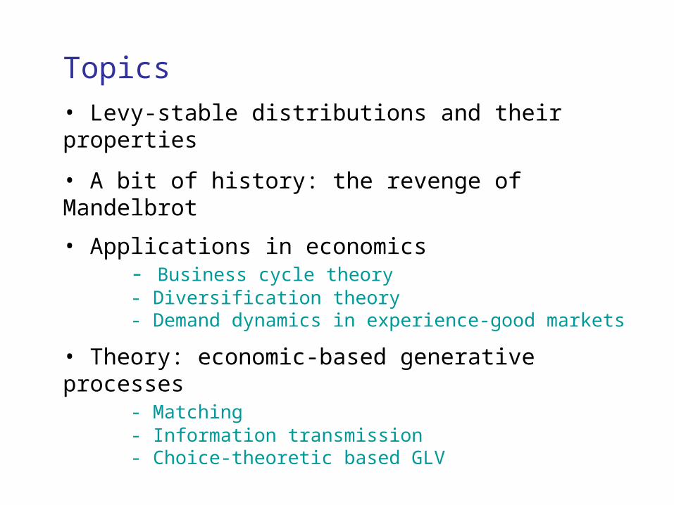
Topics• Levy-stable distributions and their properties

• A bit of history: the revenge of Mandelbrot

• Applications in economics - Business cycle theory - Diversification theory - Demand dynamics in experience-good markets

• Theory: economic-based generative processes - Matching - Information transmission - Choice-theoretic based GLV

General properties

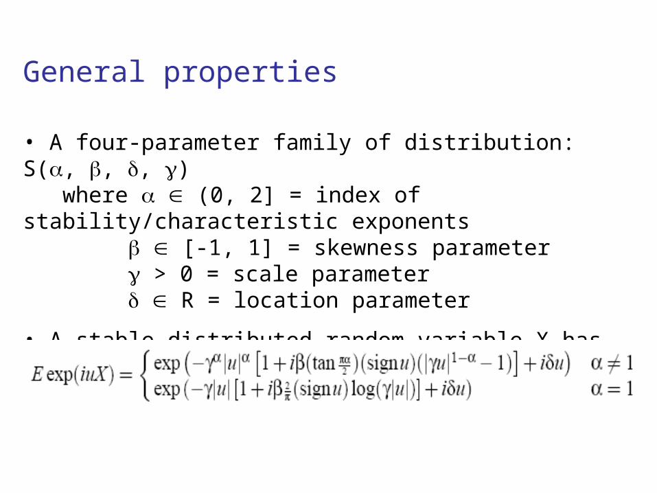
• A four-parameter family of distribution: S(, , , ) where (0, 2] = index of stability/characteristic exponents

[-1, 1] = skewness parameter > 0 = scale parameter R = location parameter

• A stable distributed random variable X has characteristic function

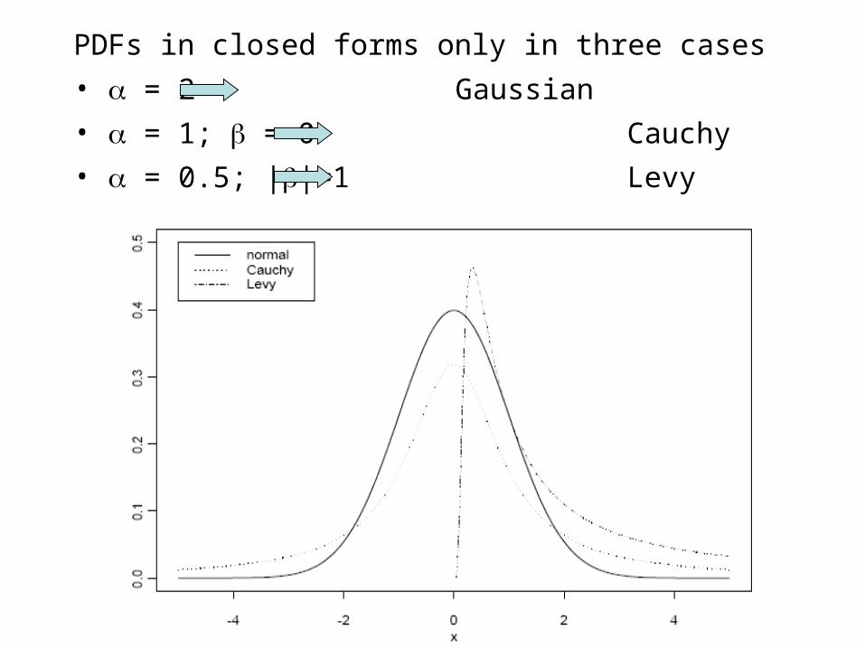
PDFs in closed forms only in three cases

• = 2 Gaussian• = 1; = 0 Cauchy• = 0.5; ||=1 Levy

Implications

• Tails are power-law distributed: P(|X| > x) ~ x

• Moments are infinite for p >

Levy-stable processes have a long history in economics

• Mandelbrot (1960`)

• The ARCH-GARCH counter-revolution (1970` - 1980`)

• The econophysics movement (1990`)

Applications in economics

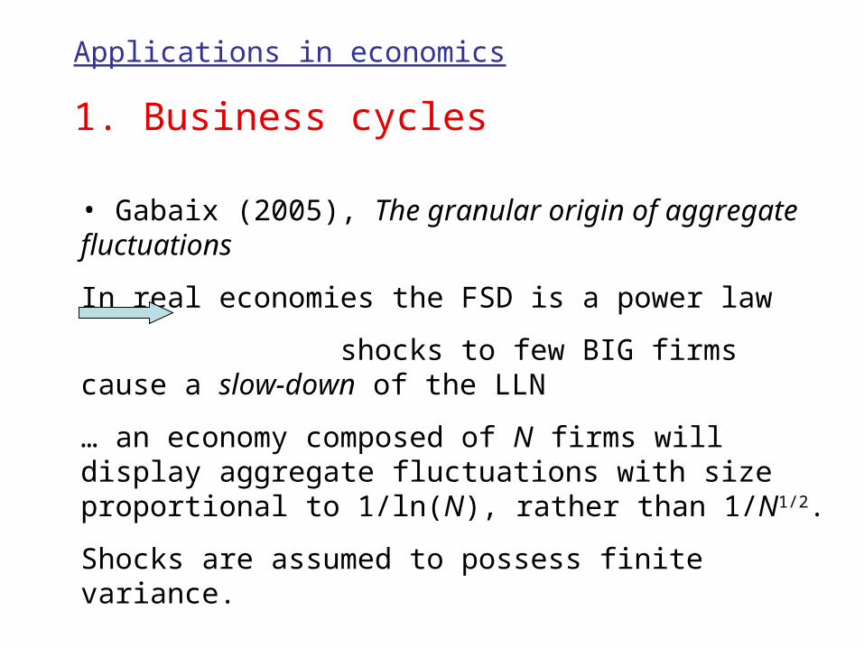
1. Business cycles

• Gabaix (2005), The granular origin of aggregate fluctuations

In real economies the FSD is a power law

shocks to few BIG firms cause a slow-down of the LLN

… an economy composed of N firms will display aggregate fluctuations with size proportional to 1/ln(N), rather than 1/N1/2.

Shocks are assumed to possess finite variance.

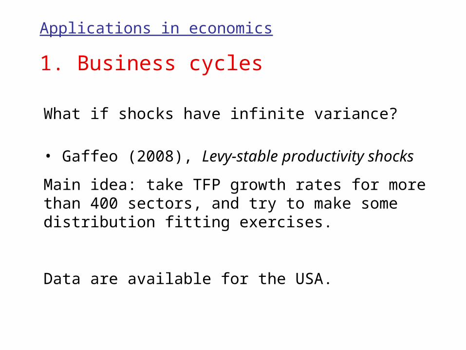
Applications in economics

1. Business cycles

What if shocks have infinite variance?

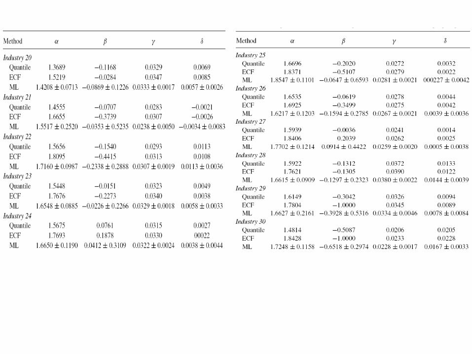
• Gaffeo (2008), Levy-stable productivity shocks

Main idea: take TFP growth rates for more than 400 sectors, and try to make some distribution fitting exercises.

Data are available for the USA.

Applications in economics

1. Business cycles

Are they just outliers?

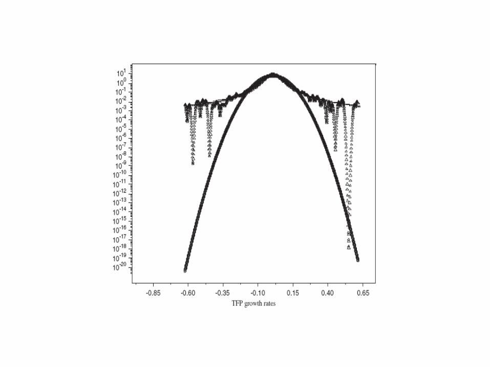
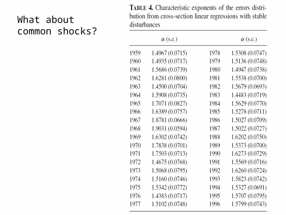
What about common shocks?

Implications for business cycles

Let us start from Hulten (1978): the rate of increase of GDP caused by iid shocks to TFP to N sectors is

If shocks have identical finite variance , and each sector is 1/N of the total, then

As the number of sectors gets large, the aggregate standard deviation becomes negligible.

Ex. If = 6% for 450 sectors, then aggregate volatility is 0.15%.

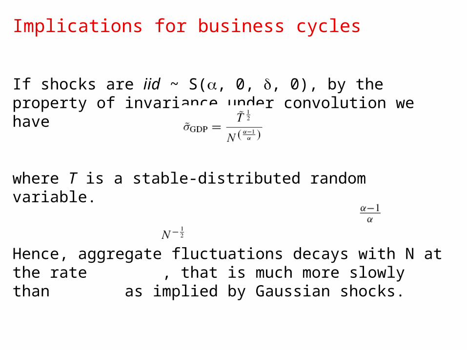
Implications for business cycles

If shocks are iid ~ S(, 0, , 0), by the property of invariance under convolution we have

where T is a stable-distributed random variable.

Hence, aggregate fluctuations decays with N at the rate , that is much more slowly than as implied by Gaussian shocks.

Applications in economics

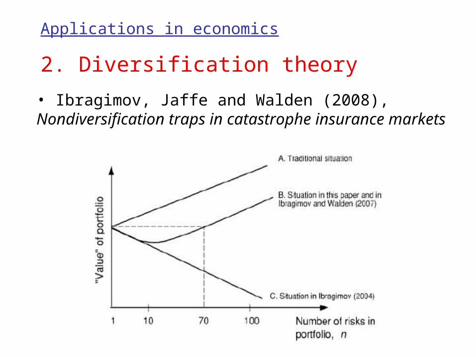
2. Diversification theory

• Ibragimov, Jaffe and Walden (2008), Nondiversification traps in catastrophe insurance markets

How much risky is our economic well-being?

Wealtht = PDVt( ) +

PDVt( W ) Present discounted value of annual interest and dividends from financial assets

Present discounted value of wages, non-corporate business and illiquid assets income Human capital and housing

10% 90%

Diversifiable in

financial markets

Is this fraction

diversifiable?

How to manage the largest economic risks?

Example: Human capital

• Construct labor income indices pricing uncertainty on future labor income;

• Design a market for labor income risk-sharing;

Problems in creating a market for labor income risk-sharing

1)Moral hazard;

2)Psychological barriers in buying insurance;

3)Microstructure of the market:- Role of intermediares

- Contract settlement - Liquidity

Ref.: Shiller (1993); Shiller and Schneider (1998).

A simple implementation

1)FIs offer insurance contracts incorporated into deposit account contracts;

2)Short position on an index related to the income from his occupation, long position on a portfolio of indices for other occupations;

3)Max overdraft facility used as a margin for labor insurance contract settlements.

Could it work?

1) Sizeable diversifiable labor income risk;

2) Careful assessment of risk distributions

- Index and option pricing- Optimal portfolio selection- Intermediaries’ risk management

A picture of the labor market in the U.S. Average hourly wages for occupations at a 4-digit level,

2006

Number of data-points: 43607

Descriptive statistics Average hourly wages for occupations in 4-digit

sectors, 2006

Mean Max Min. Std. Dev. Skewness Kurtosis Obs.[0, 20) 14.04 19.99 6.08 3.1217 0.0005 2.1073 24089[20, 40) 27.36 39.98 20.00 5.2036 0.5501 2.3223 1643[40, 60) 47.01 59.91 40.00 5.1928 0.5889 2.3216 2576[60, 80) 68.24 79.97 60.01 5.6702

0.3901 2.0573 440[80, 100) 84.34 95.46 80.00 3.6344

0.9430 3.1085 72All 21.67 95.46 6.08 11.3236 1.6994 7.0849 43607

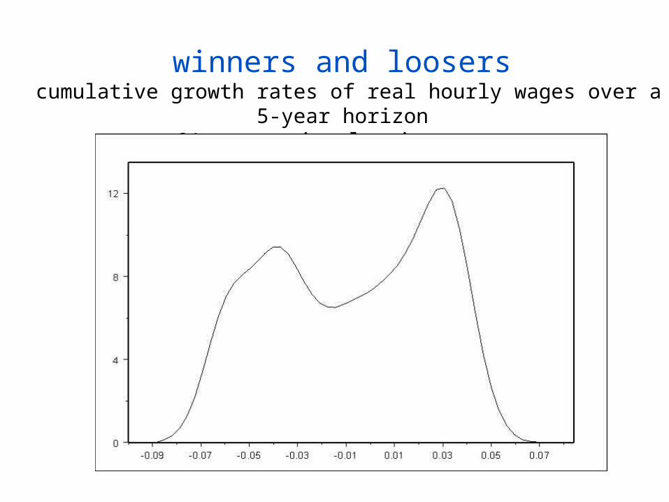
Is there enough variability? cumulative growth rates of real hourly wages over a 5-year

horizon - 293 industries

-0.16 -0.11 -0.06 -0.01 0.04 0.09 0.14 0.191

0

2

4

6

8

10

Occupational majors

1) Management2) Business and financial

operations3) Computation and

mathematical science4) Architecture and

engineering5) Life, physical and social

science6) Community and social

services7) Education, training and

library8) Art, design, entertainment,

sports and media9) Healthcare practitioner and

technical occupations10) Healthcare support

11) Protective service12) Food preparation and

serving13) Building and grounds

cleaning and maintenance14) Personal care and service15) Sales and related

occupations16) Office and administrative

support17) Farming, fishing and

forestry18) Construction and

extraction19) Installation, maintenance

and repair20) Production21) Transportation

winners and loosers cumulative growth rates of real hourly wages over a 5-year

horizon - 21 occupational major averages

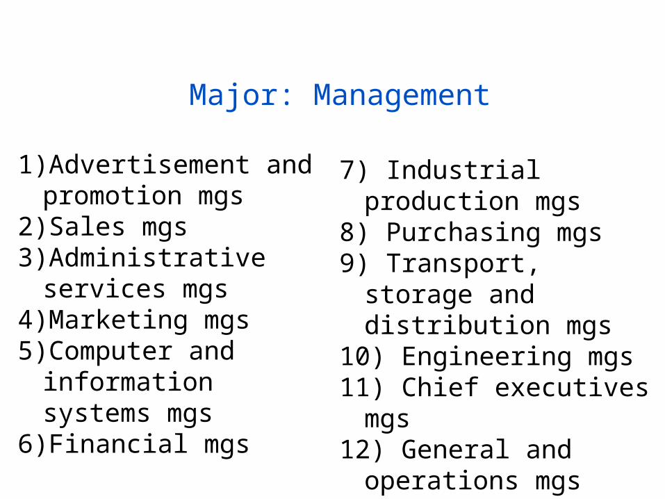
Major: Management

1)Advertisement and promotion mgs

2)Sales mgs3)Administrative

services mgs4)Marketing mgs5)Computer and

information systems mgs

6)Financial mgs

7) Industrial production mgs

8) Purchasing mgs9) Transport, storage

and distribution mgs10) Engineering mgs11) Chief executives

mgs12) General and

operations mgs

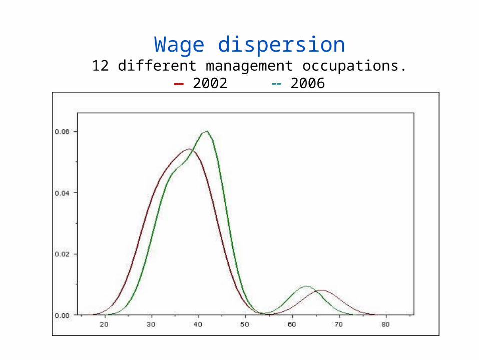
Wage dispersion12 different management occupations.

2002 2006

winners and loosers cumulative growth rates of real hourly wages over a 5-year

horizon - 12 managerial occupations

Could it work?

1) For sure, huge scope for risk-sharing;

2) Be careful in assessing the distributional features of occupational hedgeable risk

Estimation of occupation-specific growth uncertainty

g = growth rate of average occupational income over an s time horizon

z = predictable variable(s)Ref.: Athanasoulis and van Wincoop (2001).

sttittissttstti uzzgg ,,,'

,,,

Diversifiable risk

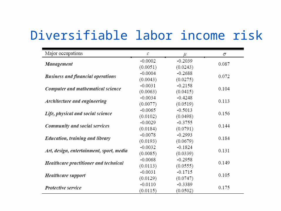
Diversifiable labor income risk (OLS)

Diversifiable labor income risk (OLS)

Diversifiable labor income risk (Levy errors)

Diversifiable labor income risk (Levy errors)

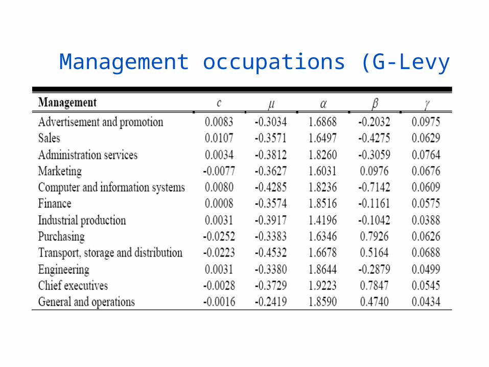
Management occupations (G-Levy errors)

Applications in economics

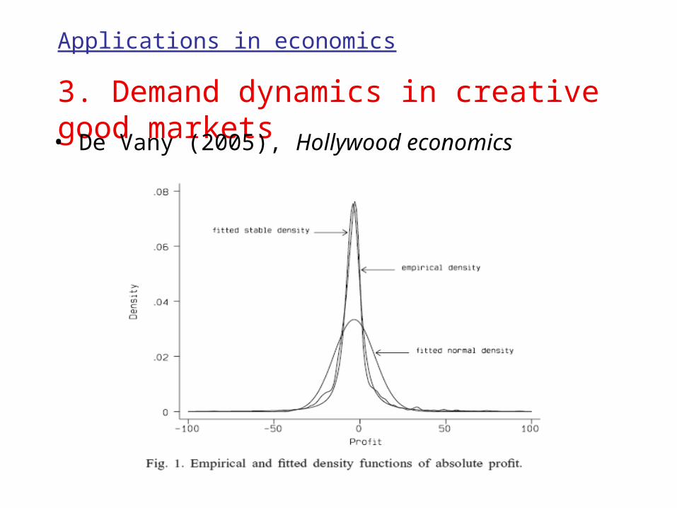
3. Demand dynamics in creative good markets• De Vany (2005), Hollywood economics

Applications in economics

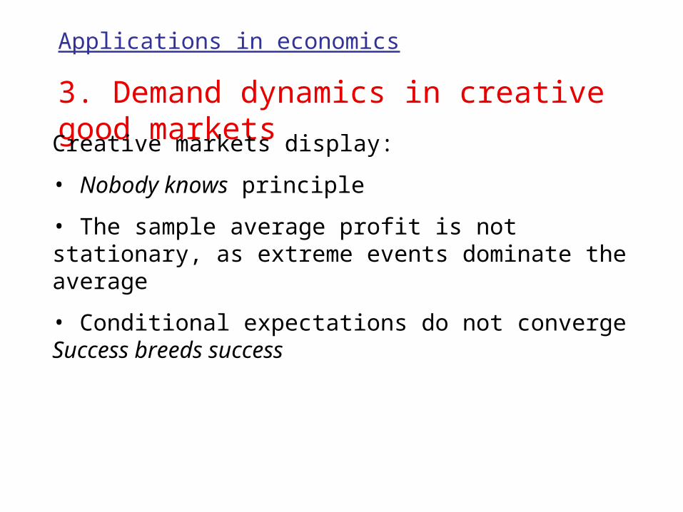
3. Demand dynamics in creative good marketsCreative markets display:

• Nobody knows principle

• The sample average profit is not stationary, as extreme events dominate the average

• Conditional expectations do not converge Success breeds success

Applications in economics

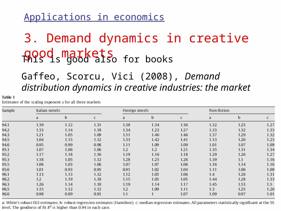
3. Demand dynamics in creative good marketsThis is good also for books

Gaffeo, Scorcu, Vici (2008), Demand distribution dynamics in creative industries: the market for books in Italy

Theory: economic-based generative processes

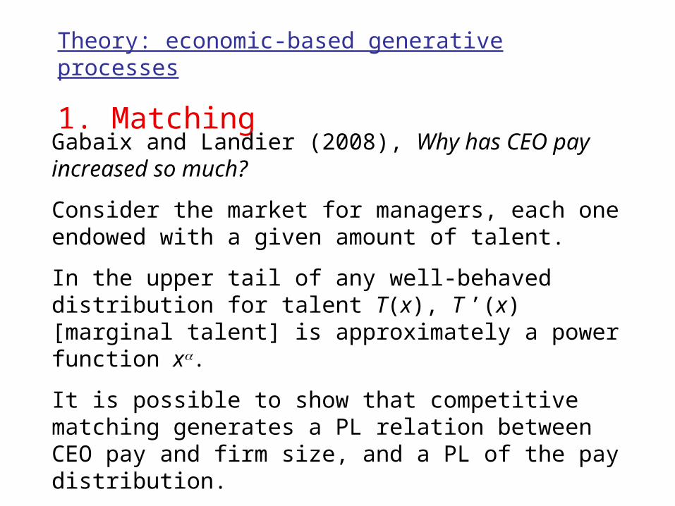
1. Matching

Gabaix and Landier (2008), Why has CEO pay increased so much?

Consider the market for managers, each one endowed with a given amount of talent.

In the upper tail of any well-behaved distribution for talent T(x), T ’(x) [marginal talent] is approximately a power function x.

It is possible to show that competitive matching generates a PL relation between CEO pay and firm size, and a PL of the pay distribution.

Theory: economic-based generative processes

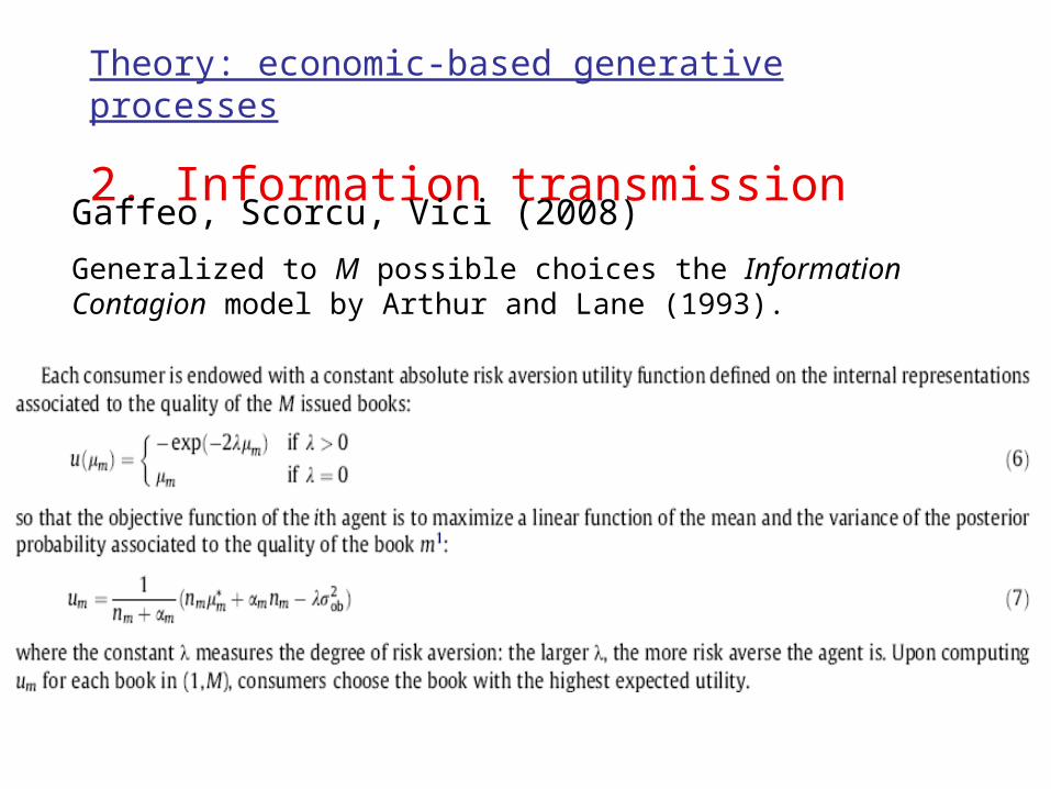
2. Information transmissionGaffeo, Scorcu, Vici (2008)

Generalized to M possible choices the Information Contagion model by Arthur and Lane (1993).

Theory: economic-based generative processes

2. Information transmissionGaffeo, Scorcu, Vici (2008)

We end up with an infinite Polya urn function.

Theory: economic-based generative processes

3. GLVDelli Gatti, Gaffeo, Gallegati (2008), A look at the relationship between industrial dynamics and aggregate fluctuations

Three basic ideas

1. The firms` financial position matters

2. Agents are heterogeneous as regards how they perceive risk associated to economic decisions

3. Firms interact through the labour and equity markets

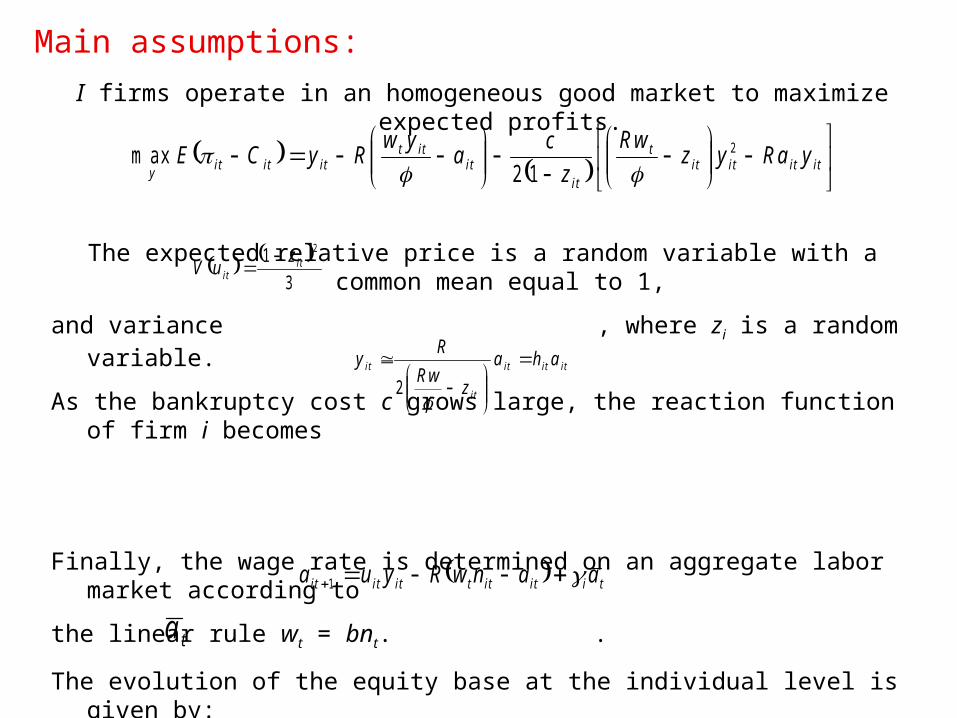
I firms operate in an homogeneous good market to maximize expected profits.

The expected relative price is a random variable with a common mean equal to 1,

and variance , where zi is a random variable.

As the bankruptcy cost c grows large, the reaction function of firm i becomes

Finally, the wage rate is determined on an aggregate labor market according to

the linear rule wt = bnt. .

The evolution of the equity base at the individual level is given by:

where is the average capitalization of firms at time t (hot market effect).

Main assumptions:

itititit

t

itit

ittititit

yyR ayz

R w

z

ca

ywRyCE 2

12m ax

3

1 2it

it

zuV

ititit

it

it aha

zR w

Ry

2

tiitittititit aanwRyua 1

ta

Solving the model

Assuming rational expectations for any i and t, as we take the cross-sectional average we obtain:

A suitable change of variable allows us to express the per-capita dynamics as:

where , and .

LOGISTIC MAP

deterministic cycles if 3 < t < 3.57

chaotic behavior if 3.57 < t < 4.

ttt

ttt aahIb

RaRha

2

22

1

ttt xxx 11

tt

t ahIb

Rx2

2

Rh tt

The rational

Aggregate behavior based on the Lotka-Volterra dynamics

During an upswing, the increase of output induces higher profits and more equity funds. Higher production means also rising

employment and higher wages, however. The increased wage bill calls for more bank loans which, when repaid, will depress

profits and the production and the equity level as well. The labour requirement thus decreases, along with the real wage, while profits raise. This restores profitability and the cycle can

start again.

The firms’ size distribution

The model can be expressed, at an individual level, as a

Generalized Lotka-Volterra system (Solomon and Levy, 1996)

The dynamics is based on

i) a stochastic autocatalytic term representing production and how it impacts on equity;

ii) a drift term representing the influence played via a hot market effect by aggregate capitalization on the financial

position of each firm

iii) a time dependent saturation term capturing the competitive pressure exerted by the labour market

The firms’ size distribution

Let be the relative equity of firm i.

It can be shown that under rather general conditions

~

with .

The distribution P() is unimodal, as it peaks at .

Above 0 it behaves like a power law with scaling exponent

below 0 it vanishes very fast.

ta

tat i

i

P

21 2

ex p

2

21

20

1

1

Implications

1) depends on:

i) how much rationed firms are in issuing new risk capital how much capital markets are affected by adverse selection and moral hazard phenomena;

ii) how much heterogeneous individuals are as regards the perceived riskyness associated to their final demand.

2) Our model suggests that the degree of industrial concentration should be country-specific.

3 , that is a proxy for agency costs in capital markets, tunes at the same time the qualitative dynamic features of aggregate fluctuations and the longitudinal characteristics of microeconomic units.

Thank you all!

Edoardo GaffeoDepartment of Economics and CEELUniversity of Trento, Italyedoardo.gaffeo@unitn.it