Level-based Incomplete LU Factorization ... - cs.odu.edupothen/Papers/ilu-levels.pdf · DISCLAIMER...

Approved for public release; further dissemination unlimited

Preprint UCRL-JC-150789

Level-based Incomplete LU Factorization: Graph Model and Algorithms

David Hysom and Alex Pothen

This article was submitted to: SIAM Journal On Matrix Analysis and Applications

November 2002

DISCLAIMER This document was prepared as an account of work sponsored by an agency of the United States Government. Neither the United States Government nor the University of California nor any of their employees, makes any warranty, express or implied, or assumes any legal liability or responsibility for the accuracy, completeness, or usefulness of any information, apparatus, product, or process disclosed, or represents that its use would not infringe privately owned rights. Reference herein to any specific commercial product, process, or service by trade name, trademark, manufacturer, or otherwise, does not necessarily constitute or imply its endorsement, recommendation, or favoring by the United States Government or the University of California. The views and opinions of authors expressed herein do not necessarily state or reflect those of the United States Government or the University of California, and shall not be used for advertising or product endorsement purposes. This is a preprint of a paper intended for publication in a journal or proceedings. Since changes may be made before publication, this preprint is made available with the understanding that it will not be cited or reproduced without the permission of the author.

This report has been reproduced directly from the best available copy.

Available to DOE and DOE contractors from the

Office of Scientific and Technical Information P.O. Box 62, Oak Ridge, TN 37831

Prices available from (423) 576-8401 http://apollo.osti.gov/bridge/

Available to the public from the

National Technical Information Service U.S. Department of Commerce

5285 Port Royal Rd., Springfield, VA 22161 http://www.ntis.gov/

OR

Lawrence Livermore National Laboratory

Technical Information Department’s Digital Library http://www.llnl.gov/tid/Library.html

LEVEL-BASED INCOMPLETE LU FACTORIZATION: GRAPHMODEL AND ALGORITHMS∗

DAVID HYSOM† AND ALEX POTHEN‡

Abstract. A graph theoretic process that models level-based, incomplete LU factorization(ILU(`)) of sparse unsymmetric matrices is developed. The model leads to two incomplete fill paththeorems that are generalizations of the original fill path theorem of Rose, Tarjan, and Lueker.Our S-level incomplete fill path theorem leads to the development of new, embarrassingly parallelalgorithms for computing the structure and storage requirements of ILU(`) factors.

Key words. ILU-factorization, graph theory, parallel algorithms

AMS subject classifications. 05C50, 05C70, 05C75, 68W10

1. Introduction. Incomplete LU factorization (ILU) is widely recognized as aneffective method for preconditioning iterative sparse linear system solvers. In general,ILU algorithms fall into one of two categories:

(i) threshold based ILUT methods;(ii) structure based ILU(`) methods.

In ILUT methods, the locations of permissible fill entries are determined in conjunc-tion with numeric factorization. Fill entries are permitted only if they are larger thana specified value, and an upper limit may be placed on the number of entries permit-ted in a row. In contrast, ILU(`) methods are separated into two phases. In the firstphase, which is often referred to as symbolic factorization, the locations of permissiblefill entries are determined. Each potential fill entry is assigned a level, and an entry ispermitted in the factor if its level is not greater than `. In the second phase, numericfactorization is performed.

In this work we are concerned with the symbolic phase of ILU(`) factorization. Wepresent a graph theoretic process that models the action of existing ILU(`) algorithms.The model is used to develop two incomplete fill path theorems that are generalizationsof the original fill path theorem that characterizes fill in complete LU factors [13, 14].

This paper is organized as follows. § 2 contains essential background material.This includes basic notation; a description of existing ILU(`) factorization algorithms;a description of the two rules (sum and max) that are commonly used to compute filllevels; and a review of the original fill path theorem for complete factorization.

In § 3 we present a graph theoretic construct that models the operation of existingILU(`) factorization algorithms.

In § 4 we use our model to prove theorems concerning structural properties ofILU(`) factors. Results include the S-level and M-level incomplete fill path theorems,which describe relationships between a fill entry’s level and paths in graphs. The

∗This work was performed under the auspices of the U.S. Department of Energy by University ofCalifornia Lawrence Livermore National Laboratory under contract number W-7405-Eng-48. UCRL-JC-150789. This research was supported in part by NSF grant DMS-9807172, by DOE SCIDAC grantDE-FC02-01ER25476, by a GAANN fellowship to the first author from the Department of Education,and by NASA under contract NAS1-19480 while the second author was in residence at ICASE.

†Center for Applied Scientific Computing, Lawrence Livermore National Laboratory, Livermore,CA, 94551 (email: [email protected]). ([email protected]).

‡Department of Computer Science, Old Dominion University, Norfolk VA 23529-0162([email protected]); and ICASE, NASA Langely Research Center, Hampton VA 23681-0001.

1

2 D. HYSOM AND A. POTHEN

S-level theorem characterizes fill that is computed using the sum rule; the M-leveltheorem characterizes fill computed using the max rule.

In § 5 we show how the S-level incomplete fill path theorem can be used todevelop novel, embarrassingly parallel algorithms for performing ILU(`) symbolic fac-torization. We show how the algorithm can be modified to compute ILU(`) storagerequirements in O(n) space, where n is the number of rows in a matrix. We in-clude summary examples that demonstrate how the S-level theorem can be used toanalytically bound fill amounts for certain classes of graphs.

In § 6 we offer some concluding remarks.

2. Background.

2.1. Preliminaries. A directed graph of a matrix G(A) = (V,E) has vertexset V , which contains a vertex for every row in the matrix, and edgeset E, whichcontains a directed edge 〈i, j〉 for every nonzero entry aij . An edge 〈i, j〉 is directedfrom i to j. G(A) is an ordered graph: if matrix row i is numbered less than matrixrow j, then vertex i is ordered before vertex j. The term filled matrix denotes thematrix F = L+U−I, where L and U are factors (either complete or incomplete) of A.The symbol F includes symmetric as well as unsymmetric cases. If A is symmetric,F = L+ LT − I, in which case U = LT .

During ILU(`) symbolic factorization, matrix entries are associated with integervalued levels. The level associated with a matrix entry fij or aij , and by extensionwith a graph edge 〈i, j〉, is denoted level(i, j).

2.2. Classical ILU(`) factorization. Figure 2.1 contains a statement of thesymbolic row-oriented Classic-ILU algorithm. By classical ILU(`) we refer to afamily of widely known and implemented algorithms that compute the structure ofILU(`) factors by mimicking direct factorization (see, for example, [15]). As in directfactorization, in their outermost loops classical ILU(`) algorithms may iterate overmatrix rows, columns, or diagonal entries. Multifrontal approaches are also possible.Since many scientific codes are equation oriented, we restrict our attention to row-oriented algorithms.

Row-oriented ILU is said to be upward looking. That is, for every nonzero entryfih with h < i, row i is updated by merging in the upper-triangular portion of thepreviously factored row h (Figure 2.1 Step 9). During this process a matrix entryfij , whose value was previously zero, may become nonzero (i.e, may “fill in”) if thereexists a nonzero entry fhj . We say the fill entry fij is caused by the existence of thetwo entries fih and fhj .

ILU(`) algorithms determine permitted fill based on the concept of a matrixentry’s level. Matrix entries in F that correspond to nonzero entries in A are assignedthe level zero (Figure 2.1, Step 6). A potential fill entry fij is assigned a level basedon the levels of its two causative entries (Figure 2.1, Step 11). If the assigned levelis not greater than `, the entry is admitted to the factor (Figure 2.1 Step 12). A fillentry may have several pairs of causative entries, and hence be assigned several levels.The convention (Figure 2.1, Step 17) is to assign a fill entry the smallest possiblelevel.

Two rules appear in the literature for assigning levels to fill entries. We referto these as the sum rule and the max rule. Assuming fij is caused by previouslyadmitted entries fih and fhj . the sum rule states

Level-based Incomplete LU factorization 3

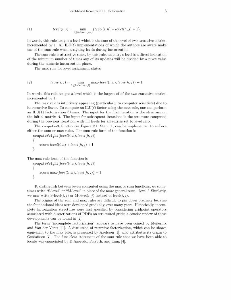
level(i, j) = min1≤h<min{i,j}

{level(i, h) + level(h, j) + 1}.(1)

In words, this rule assigns a level which is the sum of the level of two causative entries,incremented by 1. All ILU(`) implementations of which the authors are aware makeuse of the sum rule when assigning levels during factorization.

The sum rule is attractive since, by this rule, an entry’s level is a direct indicationof the minimum number of times any of its updates will be divided by a pivot valueduring the numeric factorization phase.

The max rule for level assignment states

level(i, j) = min1≤h<min{i,j}

max{level(i, h), level(h, j)}+ 1.(2)

In words, this rule assigns a level which is the largest of of the two causative entries,incremented by 1.

The max rule is intuitively appealing (particularly to computer scientists) due toits recursive flavor. To compute an ILU(`) factor using the max rule, one can performan ILU(1) factorization ` times. The input for the first iteration is the structure onthe initial matrix A. The input for subsequent iterations is the structure computedduring the previous iteration, with fill levels for all entries set to level zero.

The computeWt function in Figure 2.1, Step 11, can be implemented to enforceeither the sum or max rules. The sum rule form of the function is

computeWeight(level(i, h), level(h, j)){return level(i, h) + level(h, j) + 1

}

The max rule form of the function is

computeWeight(level(i, h), level(h, j)){return max{level(i, h), level(h, j)}+ 1

}

To distinguish between levels computed using the max or sum functions, we some-times write “S-level” or “M-level” in place of the more general term, “level.” Similarly,we may write S-level(i, j) or M-level(i, j) instead of level(i, j).

The origins of the sum and max rules are difficult to pin down precisely becausethe foundational ideas were developed gradually, over many years. Historically, incom-plete factorization structures were first specified by considering gridpoint operatorsassociated with discretizations of PDEs on structured grids; a concise review of thesedevelopments can be found in [2].

The term “incomplete factorization” appears to have been coined by Meijerinkand Van der Vorst [11]. A discussion of recursive factorization, which can be shownequivalent to the max rule, is presented by Axelsson [1], who attributes its origin toGustafsson [7]. The first clear statement of the sum rule that we have been able tolocate was enunciated by D’Azevedo, Forsyth, and Tang [4].


Classic-ILU(A, `)1 # Loop over rows2 for j = 1 to n3 # Initialization phase: admit entries in A, and assign them the level zero.4 adj′(j)← ∅5 for t ∈ adj(j)6 level(j, t)← 07 insert t in adj′(j)8 # Row-merge update phase9 for each unprocessed i ∈ adj′(j) with i < j in ascending order10 for t ∈ adj′(i) with t > i11 wt = computeWeight(level(j, i), level(i, t))12 if wt ≤ `13 if t 3 adj′(i)14 insert t in adj′(j)15 level(j, t)← wt16 else17 level(j, t)← min{level(j, t), wt)}

Fig. 2.1. Classic-ILU algorithm. The input matrix A contains n rows. The structure of arow aj∗ is represented by the list adj(j). The structure of a factor row fj∗ is represented by the listadj′(j).

2.3. The fill path theorem for complete factorization. Parter [12], andlater Rose, Tarjan, and Leuker [13, 14], developed graph theoretic vertex elimina-tion processes that model complete Gaussian Elimination. One of the highlights ofthis body of work was the development of a fill path theorem that provides a staticcharacterization of fill in F . By static we mean that the theorem permits one todetermine the location of all fill entries in F by examining paths in the graph G(A).The definition of a fill path, and a statement of the original fill path theorem follow.

Definition 1. A fill path is a path joining two vertices i and j, all of whoseinterior vertices are numbered lower than the end vertices i and j.

Theorem 2. [13, 14] Let F = L+U − I be the filled matrix corresponding to thecomplete factorization of A. Then fij 6= 0 if and only if there exists a fill path joiningi and j in the graph G(A).

Application of Theorem 2 has resulted in the gradual development of the notion ofelimination trees ([10] provides a review with many references), elimination dags [6],and many algorithms of practical importance for direct methods. For symmetric prob-lems A = LLT , algorithms exist for computing the structure of L in time proportionalto the number of nonzeros in the factor [10]. For unsymmetric problems, A = LU ,computing the structure of the L and U factors is less optimal. However, here alsoapplication of the fill path theorem has resulted in several interesting algorithms that,in practice, work quite effectively [5, 6, 13].

3. Graph Theoretic ILU(`) Model. The partial elimination process is a se-quence of graphs that models Gaussian elimination. The initial graph in the sequence,G0, is identical to the graph of the matrix, G(A) = (V,E), where all edges are as-sociated with the level zero. We assume the vertex set V contains n vertices. Thegraph Gi+1, for 0 < i ≤ n, is formed by examining all pairs of directed edges in Gi


that are directed paths of length two, and are of the form i, h, j, with h < min{i, j}.For each such path P (i, j), a directed edge 〈i, j〉 is inserted in Ei+1 if and only ifcomputeWeight(level(i, h), level(h, j)) is not greater than `. If the hypothetical edge〈i, j〉 has already been inserted, its weight is adjusted to the minimum of its presentweight and the newly calculated weight. Hence, we denote the partial eliminationprocess as

G(A) = G0, G1, G2 . . . , Gn = G∗.

For specificity, we use a superscript “S” to indicate when edge weights were cal-culated using the sum rule, e.g., GS

∗ . Similarly, a superscript “M” indicates that edgeweights were calculated using the max rule, e.g., GM

∗ .

This partial elimination process models ILU(`) factorization since matrix fill en-tries created or updated when row i is factored correspond exactly to edges insertedor updated during the formation of graph Gi. Hence we have G∗ = G(F ).

The sequence of graphs defined above differs from previous models for completefactorization in one important aspect. The models for complete factorization arebased on bordering methods, in which outer-product updates are performed whilemarching down a matrix’s diagonal. Accordingly, one vertex is eliminated (removed)from Vi during the formation of graph Gi+1 = (Vi+1, Ei+1) from graph Gi = (Vi, Ei).

Row oriented factorization requires that we leave the vertex set intact, i.e, Vi andVi+1 are identical for 0 ≤ i < n. While one can as easily formulate a graph theoreticconstruct based on bordering for incomplete factorization, such a construct wouldnot model the operation of the Classic-ILU algorithm, which is one of our primeobjectives.

4. Structural characterizations. In this section we present a collection ofdefinitions, observations, lemmas, and theorems that provide characterizations of in-complete S-level and M-level fill. We also introduce the concept of 1-alternating fillpaths, which are particular configurations of fill paths for which the S-level and M-levelcharacterizations coincide.

Figure 4.1 provides a pictorial summary of the interconnections of this section’sresults.

4.1. Static characterization of S-level fill. This section’s first result tells usthat nontrivial fill paths can always be decomposed into shorter fill paths.

Lemma 3. Any fill path P (i, j) that contains two or more edges can be uniquelydecomposed into two fill paths, P (i, h) and P (h, j), each of which contains at least asingle edge.

Proof. Given a fill path P (i, j) containing two or more edges, let h denote thehighest numbered interior vertex on the path. The P (i, h) section of this path is a fillpath by the choice of h, since all intermediate vertices on this section are numberedlower that h. Similarly, the P (h, j) section of this path is also a fill path. Thus,the fill path can clearly be decomposed in two subpaths, both of which are fill paths(existence).

To show uniqueness, suppose there exists some other decomposition. Let g bean interior vertex on the P (i, j) path, distinct from h, such that both P (i, g) andP (g, j) sections are fill paths. Then h, which is also on the P (i, j) path, must eitherbe situated between vertices i and g, or between vertices g and j. Without loss ofgenerality, assume vertex h is situated between vertices i and g. Then by Definition 1,


L3: fill path decomposition(general)

Th4: incomplete fill path theorem(S−level)

E1: sum rule

E2: max rule

graph model

classic ILU(k)

Th5: M−level edge counts

D6: bifurcated lengths

O7: fill path chording

Th8:incomplete fill path theorem(M−level)

O10: non−alternating fill paths

D9: 1−alternating fill paths

O11: fill path decomposition(internal ascending)

O12: fill path decomposition(1−alternating)

O13: fill path with 3 or fewer

O14: extending 1−alternating

edges are 1−alternating

fill paths

D1: fill path

Th2: fill path theorem

Th15: bifurcated lengths of1−alternating fill paths

Th17: equivalence of S−level andM−level for 1−alternatingfill paths

Th16: M−level(i,j) <= S−level(i,j)

Fig. 4.1. Relationships of definitions, theorems, and observations.

P (i, g) is not a fill path, since the path contains an interior vertex that is numberedhigher than one of the end vertices.

We next present the S-level incomplete fill path theorem. This theorem providesa static characterization of fill for classical ILU(`) factors that are computed usingthe sum rule for level assignment 1. The theorem is analogous to the original fill paththeorem in that it provides a means of determining fill locations by examining pathsin the graph of a matrix.

Theorem 4. Let G(A) = (V,E) be the graph of a square matrix A, and let 〈i, j〉be a permitted edge in GS

∗ . Then S-level(i, j) = k if and only if there exists a shortestfill path of length k + 1 that joins i and j in G(A).

Proof. If there is a shortest fill path of length k + 1 joining i and j in G(A), weprove the result, that an edge 〈i, j〉 with S-level(i, j) = k exists in GS

∗ , by inductionon u, which is the length of the fill path.

The base case u = 1 is immediate, since, by the construction in § 3, a fill path of

1A version of this proof was originally presented in [9].


length one in the graph G(A) is an edge 〈i, j〉 in G(A), and edges in G(A) are assignedlevel zero, and are also edges in GS

∗ .Now assume that the result is true for all lengths u less than k + 1; we show it

is also true for shortest paths of length u = k + 1. Let P (i, j) be a shortest fill pathjoining vertices i and j in G(A), and let this path have length u = k + 1.

Let h denote the highest numbered interior vertex on the fill path P (i, j). Weclaim that the P (i, h) section of this path is a shortest fill path in G(A) joining i andh. This section is a fill path by the choice of h and Lemma 3. If there were a fillpath joining i and h that was shorter than the P (i, h) section, we would be able toconcatenate it with the P (h, j) section to form a shorter P (i, j) fill path. Hence theP (i, h) section is a shortest fill path joining i and h. Similarly, the P (h, j) section ofthis path is the shortest fill path joining h and j.

Since each of these sections has fewer than k+1 edges, and is a shortest fill path,the inductive hypothesis applies. Denote the number of edges in the P (i, h) (P (h, j))section of this path by v (w), where v + w = u = k + 1. By the inductive hypothesisthe edge 〈i, h〉 is a fill edge of level v − 1 = k1, and the edge 〈h, j〉 is a fill edge oflevel w − 1 = k2. Now by the sum rule for updating fill levels, when the vertex h iseliminated, we have a fill edge 〈i, j〉 of level

k1 + k2 + 1 = (v − 1) + (w − 1) + 1 = v + w − 1 = u− 1 = (k + 1)− 1 = k.

Now we prove the converse. Suppose that 〈i, j〉 is a fill edge of level k in GS∗ ; we

show the result that there exists a shortest fill path in G(A) containing u = k + 1edges by induction on the level k.

The base case k = 0 is immediate since, by the construction in § 3, the edge 〈i, j〉constitutes a trivial fill path of length one.

Assume that the result is true for all fill levels less than k. Let the fill edge 〈i, j〉with S-level(i, j) = k be created in GS

∗ , when vertex h is eliminated, by the previouslyexisting edges 〈i, h〉 and 〈h, j〉. Let the edge 〈i, h〉 have level k1 and the edge 〈h, j〉have level k2. By the sum rule for computing levels, we have that k1 + k2 + 1 = k.By the inductive hypothesis, there is a shortest fill path of length v = k1 + 1 joiningi and h, and such a path of length w = k2 + 1 joining h and j. Concatenating thesepaths, we find a fill path joining i and j of length

v + w = (k1 + 1) + (k2 + 1) = k1 + k2 + 2 = k + 1.

We need to prove that the P (i, j) fill path in the previous paragraph is a shortestfill path between i and j. Consider any other pair of edges 〈i, g〉 and 〈g, j〉 in GS

i thatcauses the fill edge 〈i, j〉 when vertex i is eliminated. By the choice of the vertex h, ifthe level of the edge 〈i, g〉 is k′1, and that of 〈g, j〉 is k′2, then k′1 + k′2 ≥ k.

The inductive hypothesis applies to the P (i, g) and P (g, j) sections, and hencethe sum of their lengths is at least k + 1.

D’Azevedo, Forsyth, and Tang [4] were aware of the connection between matrixentry levels and fill path lengths in graphs. However, they framed the connection asa definition for all fill levels. We quote from their work.

We define the fill level for the node pair (vi, vj) in Gk to be the length

of the shortest path from vi to vj minus one, i.e. level(k)ij = m We

define initially

level(0)ij =

{

0 if aij 6= 0∞ otherwise.


1

23

3

8

2

1

4

1

1

1

1

2

3

2

8 9

4

6

3

5

1

7

2

Fig. 4.2. M-level fill level and path length relationships. Edges in G(A) are drawn with solidlines. Edges in GM

∗ are drawn with dashed lines, and labeled with their levels. The vertex numberingindicates elimination ordering. Both graphs contain an M-level k = 3 fill edge. The correspondingfill path in the graph on the left, 8,1,2,3,4, contains 3 + 1 = k + 1 = 4 edges. The corresponding fillpath in the graph on the right, 8,1,5,2,7,3,6,4,9, contains 23 = 2k = 8 edges.

In contrast, we start with a weaker premise—the definition of level zero fill—thenprove an if and only if connection.

D’Azevedo, Forsyth, and Tang’s work centers around a novel algorithm that com-bines an ordering technique with ILU factorization. They consider G(A) to be initiallyunordered, and one vertex is ordered during each elimination step. They define filllevels in terms of path lengths through vertices in reachable sets, with a reachableset consisting of vertices already eliminated and ordered. They did not postulate orprove this connection as a theorem, as we have done.

4.2. Static characterization of M-level fill. We now turn our attention to-wards M-level fill entries and their associated fill paths. While a fill edge withS-level(i, j) = k corresponds to a fill path with exactly k + 1 edges, this section’sfirst result says that a fill edge with M-level(i, j) = k corresponds to a fill path thatmay contain anywhere between k+1 and 2k edges. Figure 4.2 illustrates the intuitionunderlying this claim. Two very simple graphs are shown, both of which contain fillpaths that correspond to level k = 3 fill edges. The fill path in the Figure 4.2(a) con-tains 3+1 = k+1 = 4 edges, while the fill path in Figure 4.2(b) contains 23 = 2k = 8edges.

Theorem 5. Let G(A) = (V,E) be the graph of a square matrix A, let 〈i, j〉 be apermitted edge in GM

∗ with M-level(i, j) = k, and let P (i, j) be a shortest fill path inG(A). Let u represent the number of edges in the path P (i, j). Then k+1 ≤ u ≤ 2k.

Proof. We argue by induction on the fill edge’s level, k. The base case k = 0 isimmediate since, by the construction specified in § 3, a fill edge of level zero corre-sponds to a fill path that contains u = 1 edges. In this case k + 1 = 1 ≤ u ≤ 2k = 1,so the result is true.

Now assume the result is true for all edges whose M-level is less than k; we showit is also true for edges with level k. Let h be the vertex whose elimination creates thefill edge 〈i, j〉 of M-level k. Let the edge 〈i, h〉 have M-level k1 and the edge 〈h, j〉 haveM-level k2. By the max rule for computing levels, we have that max{k1, k2}+ 1 = k,


hence both k1 and k2 are less than k, so the inductive hypothesis applies. Also, eitherk1 = k − 1 or k2 = k − 1 or both. Without loss of generality, assume k1 = k − 1.

Let v represent the number of edges in the fill path joining i and h in G(A), andw the number of edges in the fill path joining h and j in G(A). By the inductivehypothesis, k1 + 1 ≤ v ≤ 2k1 , and k2 + 1 ≤ w ≤ 2k2 . When h is eliminated thesepaths are concatenated, resulting in the fill path P (i, j) whose length u is bounded:

(k1 + 1) + (k2 + 1) ≤ u ≤ 2k1 + 2k2 .

To make the left-hand side as small as possible, assume k1 = k − 1 and k2 = 0,which is possible if P (h, j) contains a single edge. In this case

u = (k1 + 1) + (k2 + 1) = ((k − 1) + 1) + (0 + 1) = k + 1.

To make the right-hand side as large as possible, let k1 = k − 1 and k2 = k − 1.In this case

u = 2k1 + 2k2 = 2(k−1) + 2(k−1) = 2k.

Therefore, k + 1 ≤ u ≤ 2k.Not only is there wide latitude in fill path lengths associated with M-level fill

edges, but it is also the case that a fill path P (i, j) in G(A) that is associated with afill edge 〈i, j〉 in GM

∗ may not be the shortest fill path (that is, the fill path containingthe fewest number of edges) that connects vertices i and j in G(A). Figure 4.3illustrates this point. The figure shows a fill edge with M-level(i, j)=3 that arises dueto the existence of a fill path that contains eight edges. Vertices i and j are alsoconnected by a fill path that only contains five edges; however, this fill path wouldcause 〈i, j〉 to have M-level(i, j) = 4.

Hence, when fill is computed using the max rule, it appears that there is nonecessary connection between fill levels and path lengths (where “length” indicates,as we use the term, the number of edges in a path). These observations suggest theneed for a definition of path length that does not strictly depend on the number ofedges in the path. Accordingly, we introduce the concept of bifurcated length, whichis recursive in nature. In the following definition the phrase “unique fill subpaths”refers to the unique decomposition stated in Lemma 3.

Definition 6. A fill path containing a single edge has bifurcated length zero.A fill path containing two or more edges, whose unique fill subpaths have bifurcatedlengths v and w, has bifurcated length u = max{v, w}+ 1.

Heretofore, we have used the phrase “shortest fill path” to indicate, of all possiblefill paths connecting two vertices in a graph, a (possibly nonunique) path containingthe fewest number of edges. When discussing bifurcated lengths we use an analogousphrase, “fill path with shortest bifurcated length.” This term indicates, of all possi-ble fill paths connecting two vertices in a graph, a (possibly nonunique) path whosebifurcated length is the smallest possible.

A chord of a path is an edge that joins two non-consecutive vertices on the path.If an edge is added to a graph such that the shortest fill path P (i, j) is chorded, theresult will be that vertices i and j are joined by a shorter fill path than previously, andhence the corresponding S-level(i, j) will be reduced. This concept does not transferto the study of bifurcated path lengths.

Observation 7. A fill path may be chorded, and its bifurcated length unchanged.


i

j

i

j

i

j

1

1 1

1

2 2

3

12

3

4

Fig. 4.3. M-level path lengths and edge counts. Top: a graph in which vertices i and j areconnected by two fill paths. In the middle and bottom, the paths are shown separately, with fill edgesindicated by dashed lines. The path in the middle contains fewer edges but results in a fill edgethat has a higher level than does the path at the bottom. Vertex ordering is indicated by verticalplacement: vertices that are lower on the page are assumed to be ordered before vertices placed higheron the page.

Figure 4.4 shows a fill path that contains 8 edges and has bifurcated length 4.After chording, the resulting shorter fill path contains only 7 edges, however, itsbifurcated length is unchanged.

The next theorem provides a static characterization of M-level fill.

Theorem 8. Let G(A) = (V,E) be the graph of a square matrix A, and let 〈i, j〉be a permitted edge in GM

∗ . Then M-level(i, j) = k if and only if there exists a fill


i i

1

12 2

33

4

12 1

23

4j

j

t1

t2

t3

t4

t5

t6

t7 t1

t2

t3

t4

t5

t6

t7

Fig. 4.4. A fill path may be chorded, and its bifurcated length unchanged. Left: fill pathP (i, j) = i, t1, t2, t3, t4, t5, t6, t7, j in G(A) contains 8 edges and has bifurcated length 4. Right: thesub path t5, t6, t7 has been chorded in G(A); i and j are now connected by the shorter fill pathP (i, j) = i, t1, t2, t3, t4, t5, t7, j. This path contains 7 edges, but the bifurcated length of P (i, j)remains 4. Edges in G(A) are drawn with solid lines. Edges in GM

∗ are drawn with dashed lines,and labeled with their levels. Vertex ordering is indicated by vertical placement: vertices that arelower on the page are assumed to be ordered before vertices placed higher on the page.

path joining vertices i and j in G(A) with bifurcated length k, and this path has theshortest bifurcated length amongst all fill paths between i and j.

Remark. In contrast to Theorem 4, here there is no “+1” difference betweenbifurcated path lengths and M-levels. This is because the “+1” is incorporated intothe definition of bifurcated path lengths.

Proof. If there is a fill path with shortest bifurcated length k joining i and j inG(A), we prove the result, that an edge 〈i, j〉 with M-level(i, j) = k exists in GM

∗ , byinduction on u, which is the bifurcated length of the fill path.

The base case u = 0 is immediate, since, by the construction in § 3 and Defini-tion 6, a path with bifurcated length zero corresponds to an original edge in G(A).

Now assume the result is true for all fill paths with bifurcated length u less thank. We will prove that the result is true when the bifurcated length of a fill path isu = k.

Let P (i, j) be a fill path with shortest bifurcated length that joins i to j in G(A),and let the bifurcated length of this path be u = k. Let h be the highest-numberedinterior vertex in this fill path. Then P (i, h) and P (h, j) are also fill paths by Lemma 3.

Let the bifurcated length of the fill path P (i, h) be v and let the bifurcated lengthof the fill path P (h, j) be w. By Definition 6, the bifurcated path length of P (i, j) ismax{v, w}+ 1, so the bifurcated lengths of v and w are both less than k. Note thateither v or w (or both) is equal to k − 1. Without loss of generality, assume that wis less than k − 1. Then it must be that v = k − 1, and therefore the fill path P (i, h)has the shortest bifurcated length possible.

Now suppose there is a path P ′(h, j) whose bifurcated length is less than w. Thenwe can freely replace the path P (h, j) with the path P ′(h, j), and the bifurcated lengthof the path P (i, j) will be unchanged.

Thus P (i, j) is decomposable into two subpaths, P (i, h) and P (h, j), both of whichare fill paths and have shortest bifurcated lengths less than k. Hence, the inductivehypothesis applies, so there exists a fill edge 〈i, h〉 with M-level v, and a fill edge 〈h, j〉with M-level w. By the max level rule, when vertex h is eliminated, the fill edge 〈i, j〉


is created with M-level(i, j) = max{v, w}+ 1 = k.Now we prove the converse. Suppose that 〈i, j〉 is a fill edge with M-level(i, j) = k

in GM∗ ; we show the result that there exists a fill path P (i, j) in G(A) with shortest

bifurcated length u = k by induction on k, the edge’s level.The base case k = 0 is immediate since, by the construction in § 3, a fill edge with

level zero corresponds to a fill path that contains a single edge, and by Definition 6this path has bifurcated length zero.

Now assume the result is true for all fill edges with M-level less than k; we showit is also true for fill edges with M-level equal to k.

Assume the fill edge 〈i, j〉 with M-level(i, j) = k is created, when vertex h iseliminated from GM

h , by the previously existing edges 〈i, h〉 and 〈h, j〉.Let the edge 〈i, h〉 have M-level(i, h) = k1 and the edge 〈h, j〉 have

M-level(h, j) = k2. By the max rule for computing levels, we have that max{k1, k2}+1 = k. Then both fill edges 〈i, h〉 and 〈h, j〉 have levels less than k, so the inductivehypothesis applies. Thus there exists a fill path that connects vertices i and h and hasshortest bifurcated length v = k1, and a fill path that connects vertices h and j andhas shortest bifurcated length w = k2. Additionally, either k1 = k − 1 or k2 = k − 1or both. Without loss of generality, assume k1 = k − 1.

Now from Definition 6, the bifurcated length of the fill path P (i, j) is

u = max{v, w}+ 1 = max{k1, w}+ 1 = max{k − 1, w}+ 1 = k.

We also need to prove that the P (i, j) fill path has the shortest bifurcated lengthamongst all fill paths connecting vertices i and j in G(A). Suppose there were a pathP ′(i, j) in G(A) that had a shorter bifurcated length, that is, a bifurcated lengthu′ less than k. From the first part of this proof, the edge 〈i, j〉 in GM

∗ would thenhave an M-level less than k, which contradicts the premise that the fill edge 〈i, j〉 hasM-level(i, j) = k.

4.3. Similarity of S-level and M-level fill for 1-alternating fill paths.A graph sometimes has the property that an ILU(`) factorization computed usingthe sum rule is identical to that which results when the max level is used. Thisproperty is an attribute, e.g., of graphs whose associated matrices arise from thediscretization of partial differential equations on naturally ordered, structured grids,when the factorization level is ` ≤ 3. For these graphs, the shortest fill path connectingany two vertices i and j, and the fill path with shortest bifurcated length connectingthe same two vertices i and j, are always identical when level(i, j) ≤ 3. A consequence(which is the main result of this section) is that M-level(i, j) = S-level(i, j) for suchcases. To capture and generalize the particular feature responsible for this consonanceof level assignment, we define 1-alternating fill paths.

As a preliminary, an ascending path is a path (t1, . . . , tk) that contains at leasttwo vertices, with th < th+1 for 1 ≤ h < k. Similarly, a descending path is a path(t1, . . . , tk) that contains at least two vertices, with th > th+1 for 1 ≤ h < k.

Definition 9. A fill path P (i, j) is 1-alternating if it has one of the followingforms.(i) A single edge, 〈i, j〉.(ii) An edge 〈i, h〉 with i > h, concatenated with an ascending path P (h, j).(iii) A descending path P (i, h) concatenated with an edge 〈h, j〉 with h < j.(iv) A descending path P (i, h) concatenated with an ascending path P (h, j).

Note that forms (ii) and (iii) are restricted forms of form (iv). We call a 1-alternating path internal-ascending if it is either of form (ii), or consists of a single


i

j

t1

t2

t3

i

j

t1

t2

t3

i

t1

t2

t3

ij

t1

t2

t3

j

Fig. 4.5. 1-alternating and non-alternating fill paths. Top left: internal-ascending fill path.Top right: internal-descending fill path. Bottom left: 1-alternating fill path. Bottom right: non-alternating fill path. Here as elsewhere, vertical positioning of vertices is indicative of their relativeorderings.

edge 〈i, j〉 with i < j. We call a 1-alternating path internal-descending if it is eitherof form (iii), or consists of a single edge 〈i, j〉 with i > j. Figure 4.5 illustrates thedifferent species of 1-alternating fill paths, and the difference between 1-alternatingand non-alternating fill paths.

By way of building up to this section’s main result, and as an aid to intuition,several observations concerning properties of 1-alternating fill paths follow.

Observation 10. A fill path is non-alternating if the path contains a sequenceof interior vertices, tf , . . . , tg, . . . , th, such that tf < tg and tg > th.

In the non-alternating path at the bottom right of Figure 4.5, t1 < t2 and t2 > t3.

Observation 11. If P (i, j) = i, t1, t2, . . . , j is an internal-ascending fill path thatcontains at least three edges, and h is any interior vertex on the path with h > t1,then P (i, h) is also an internal-ascending fill path.

The truth of this observation follows immediately from Definitions 1 and 9. Re-ferring to the P (i, j) fill path illustrated in the top left portion of Figure 4.5, thisobservation says that the paths P (i, t2) and P (i, t3) are internal-ascending fill paths.Note, however, that neither P (t1, j) nor P (t2, j) is a fill path. A similar observationholds for internal-descending paths.

The next observation is based on the fact that the highest numbered interiorvertex of a 1-alternating path is necessarily adjacent to one of the end points of thepath.


Observation 12. If P (i, j) is a 1-alternating fill path containing k + 1 edges,with k ≥ 1, then the path can be uniquely decomposed into two 1-alternating fill pathsP (i, h) and P (h, j). One of these fill paths will contain k edges, and the other a singleedge.

The existence and uniqueness of the decomposition was shown in Lemma 3. Inthat lemma’s proof, we saw that the vertex h is necessarily the largest interior vertexon the P (i, j) path. From Definition 9, this vertex is adjacent to either vertex i orvertex j, hence either P (h, j) is a path containing a single edge, in which case thepath P (i, h) must contain k edges, or P (i, h) is a path containing a single edge, inwhich case the path P (h, j) must contain k edges. Referring again to Figure 4.5, theP (i, j) fill path in the top left contains four edges, and can be decomposed into thefill paths (i, t3) and (t3, j), containing three edges and a single edge, respectively.

Observation 13. Any fill path with three or fewer edges is 1-alternating.

The truth for the one and two edge cases follows directly from Definition 9. Nowconsider a fill path with three edges, i, t1, t2, j. Either t1 < t2, or t2 < t1; in eithercase the fill path is 1-alternating by Definition 9. As illustrated in the bottom rightof Figure 4.5, paths with four or more edges are not necessarily 1-alternating.

Observation 14. If P (i, j) is any species of 1-alternating fill path, then(i) if 〈j, t〉 is an edge with j < min{i, t}, then P (i, t) is also a 1-alternating fill path;(ii) if 〈t, i〉 is an edge with i < min{j, t}, then P (t, j) is also a 1-alternating fill path.

In the top left of Figure 4.5, P (i, t3) is a 1-alternating fill path, and 〈t3, j〉 isan edge. By this observation, P (i, j) is therefore a 1-alternating fill path. Thisobservation states a condition that permits a fill path to be extended while preservingits 1-alternating character. As such it is the complement of Observation 12, whichsays that any 1-alternating fill path can be decomposed.

Note that extending a 1-alternating path does not necessarily preserve anyinternal-descending or internal-ascending property it may possess. For example, ifan internal-descending fill path P (i, j) is extended by concatenation with an edge〈j, t〉 with t > j, then the resulting fill path P (i, t) is no longer internal-descending.

The following theorem establishes a relationship between path lengths and bifur-cated lengths of 1-alternating fill paths.

Theorem 15. Let P (i, j) be a fill path that contains k + 1 edges. The bifurcatedlength of P (i, j) is k if and only if the fill path is 1-alternating.

Proof. Suppose there exists a 1-alternating fill path that connects vertices i andj and contains k + 1 edges. We prove the path has bifurcated length k by inductionon k, the number of edges in the path.

The base case k = 0 is immediate since a fill path containing a single edge has bi-furcated length zero by Definition 6. Now assume the result is true for all 1-alternatingfill paths containing k or fewer edges; we show it is also true for 1-alternating fill pathscontaining k + 1 edges.

Let h denote the highest numbered interior vertex on the path joining i and j.From Observation 12, h must be adjacent to either vertex i or vertex j. Without lossof generality, assume it is adjacent to vertex j.

Thus, P (i, h) is a 1-alternating fill path containing k edges, and P (h, j) is a 1-alternating fill path containing a single edge, so the inductive hypothesis applies toboth subpaths.

By the inductive hypothesis, P (i, h) has bifurcated length k − 1, and P (h, j) hasbifurcated length zero. When these two paths are concatenated, the resulting pathP (i, j) has bifurcated length, by Definition 6, of


max{k − 1, 0}+ 1 = k.

Now we prove the converse. Suppose vertices i and j are connected by a fillpath that contains k+ 1 edges and has bifurcated length k; we show that the path is1-alternating by induction on k, the number of edges in the path.

The base case k = 1 is immediate since a fill path containing a single edge is1-alternating (Definition 6). Now assume the result is true for any fill path thatcontains m edges and has bifurcated length m− 1, where m ≤ k. We show the resultis also true for paths that contain k + 1 edges.

Let h denote the highest numbered interior vertex on the fill path joining i and j.Let m1 be the number of edges in the P (i, h) subpath, and m2 the number of edgesin the P (h, j) subpath. Then m1 +m2 = k + 1.

Let k1 be the bifurcated length of the P (i, h) subpath, and k2 be the bifurcatedlength of the P (h, j) subpath. Then max{k1, k2} + 1 = k. Hence, either k1 = k − 1or k2 = k − 1 or both. Without loss of generality, suppose k1 = k − 1. Then fromTheorem 5, the P (i, h) subpath must contain at least k edges, that is, m1 ≥ k. Andsince m1+m2 = k+1, it must contain exactly k edges, and m2, the number of edgesin the P (h, j) subpath, must be 1.

Since P (i, h) has bifurcated length k − 1 and contains k edges, the inductivehypothesis applies, i.e, P (i, h) is a 1-alternating fill path. Similarly, since P (h, j)contains a single edge, and by definition 6 has bifurcated length zero, the inductivehypothesis applies.

Finally, by Observation 14, when the P (i, h) path is concatenated with the P (h, j)path, the resulting P (i, j) fill path is 1-alternating.

The next observation tells us that the M-level associated with a fill path is nevergreater than the S-level associated with that same path.

Observation 16. Let G(A) = (V,E) be the graph of a square matrix A, and letM-level(i, j) = k. Then S-level(i, j) ≥M-level(i, j).

From the left hand side inequality of Theorem 5, any fill path P (i, j) must containat least k+1 edges. The truth of the preceding observation then follows directly fromTheorem 4.

This section’s final theorem formalizes the relationship between M-level andS-level fill that was alluded to in this section’s introduction.

Theorem 17. Let G(A) = (V,E) be the graph of a square matrix A, and let 〈i, j〉be a permitted edge in GM

∗ with M-level(i, j) = k. Then M-level(i, j) = S-level(i, j) ifand only if there exists a fill path with shortest bifurcated length connecting i and jthat is also 1-alternating.

Proof. Suppose M-level(i, j) = S-level(i, j); we show there must exit a fill pathwith shortest bifurcated length connecting i and j that is also 1-alternating.

By the supposition that S-level(i, j) = k and Theorem 4, there exists a fill pathP (i, j) connecting i and j that has k + 1 edges. By the same theorem, no fill pathconnecting i and j can have fewer than k + 1 edges.

By the supposition that M-level(i, j) = k and Theorem 8, no fill path connectingi and j can have bifurcated length shorter than k. In particular, the bifurcated lengthof P (i, j) can not be shorter than k.

By Observation 16, the M-level value derived from any fill path can not be greaterthan the S-level derived from that path. Hence, the bifurcated length of P (i, j) cannot be longer than k.


Since the bifurcated length of P (i, j) can be neither longer nor shorter than k, itmust be equal to k, and since no fill path connecting these two nodes can have shorterbifurcated length, P (i, j) must be a fill path with shortest bifurcated length. Sincethe path contains k + 1 edges, by Theorem 15 it is 1-alternating.

Now we prove the converse. Suppose there exists a fill P (i, j) with shortestbifurcated length k that is also 1-alternating; we show that M-level(i, j) = S-level(i, j).

By Theorem 8, M-level(i, j) = k, so we must show that S-level(i, j) = k; byTheorem 4, it suffices to show that there exists a shortest fill path connecting nodesi and j that contains k + 1 edges.

Since M-level(i, j) = k, by Theorem 5 every fill path connecting nodes i and jcontains at least k + 1 edges. It therefore suffices to show that P (i, j) contains k + 1edges. We can now restate our goal as follows.

Suppose there exists a fill path P (i, j) with bifurcated length k that is also 1-alternating; we show that this path contains k + 1 edges by induction on u, thebifurcated length of the fill path.

The base case, u = 0, is immediate, from Definitions 6 and 9. Now assume theresult is true for all values of u < k; we show the result is also true for u = k.

By Observation 12, P (i, j) can be decomposed into two fill paths, P (i, h) andP (h, j), both of which are 1-alternating. One of these paths is exactly one edge long,so the inductive hypothesis applies. Without loss of generality, assume this edge isP (i, h).

By Definition 6, the bifurcated length of P (h, j) must be u = k − 1. If it werenot, then when fill paths P (i, h) and P (h, j) were joined, the resulting fill path wouldnot have a bifurcated length of k, as was supposed. Since P (h, j) is 1-alternating andhas bifurcated length u < k the hypothesis applies, so the path contains u + 1 = kedges. Then when P (i, h) and P (h, j) are concatenated, the result is P (i, j), whichcontains k + 1 edges.

5. Applications. This section provides a brief overview of some of the practicalapplications of the S-level incomplete fill path theorem. Additional applications anddetailed explanations can be found in [8].

5.1. Computing upper triangular structures. Figure 5.1 shows a procedure,GS-Urow, that can be used to compute ILU(`) structures that are identical to thosecomputed by Classic-ILU. The procedure is invoked separately for each row in thematrix. Unlike Classic-ILU, which requires the results of previously computed rows1 through i − 1 to factor a row i, the new GS-Urow procedure requires only thegraph G(A), and hence has the novel feature that the structure of each row in thefactor can be computed independently, in parallel.

The procedure operates via a simple breadth first search [3] that finds a shortestpath between a seed vertex i and vertices reachable from i via traversal of ` + 1 orfewer edges. Hence, the correctness of the algorithm follows directly from Theorem 4.Other algorithms can be devised that compute the structure of rows in the lowertriangular factor; see [8] for details.

For structured 3D graphs, it can be shown that GS-Urow has a lower runtimecomplexity (O(n`3/p)) than does Classic-ILU (O(n`4)). (Here, p is the number ofprocessors, n is the number of rows in the matrix, and ` is the factorization level.)For structured 2D graphs, runtimes are (O(n`2/p)) for GS-Urow and (O(n`2)) forClassic-ILU [8].


GS-Urow(G(A), `, i, adj′(i))1 # Initialization for BFS from vertex i2 Q← {i}3 length[i]← 04 visited[i]← i5 # BFS phase6 while Q 6= ∅7 h← Dequeue(Q)8 for t ∈ adj(h) with visited[t] 6= i9 visited[t]← i10 if t < i and length[h] < `11 Enqueue(Q, t)12 length[t] = length[h] + 113 if t > i14 insert t in adj′(i)

Fig. 5.1. GS-Urow. This procedure computes the structure of row i in the the factor’s uppertriangle. Inputs are G(A); `, the factorization level; and i, the row whose structure is to be computed.The row’s structure is returned in adj′(i)).

5.2. ILU(`) memory allocation. As noted in §2.3, it is possible to computestorage requirements for factors of symmetric matrices in time proportional to thenumber of nonzeros in F , and in space proportional to the row count. This enables oneto efficiently allocate storage and set up data structures prior to the commencementof numeric factorization.

In general, there is no equivalent procedure for predicting ILU storage require-ments. One practice is to guess at the number of nonzeros in the factor and initiallyallocate that much storage; if this proves insufficient, the factorization fails. In someILU schemes, such as ILUT, an arbitrary limit is set on the number of nonzeros ineach row. This ensures that adequate storage will be allocated and, unless a zero-pivot is encountered, the factorization will succeed. Another approach, common inimplementations coded in C or C++, is to dynamically reallocate storage when theinitial guess is insufficient. However, this reallocation strategy can incur non-trivialoverhead and can also fragment memory.

The GS-Urow procedure presented in the previous section (Figure 5.1) can bemodified to compute storage requirements for ILU(`) upper triangular factors usingO(n) space. The modification is accomplished as follows. Initialize a counter tozero. Change Step 14, which previously inserted an element in an adjacency list, toincrement the counter. Return the counter’s value.

While these modifications permit computation of a factor’s storage requirementsin O(n) space, the time complexity is identical to that required for actually performingsymbolic factorization. It is an open question whether faster methods for computingexact ILU(`) storage requirements can be devised.

5.3. Bounding ILU(`) fill amounts. The S-level incomplete fill path theoremcan be used as an analytic tool to bound the amount of fill in ILU(`) factors. The coreidea is to devise an expression that bounds the number of vertices that are reachablefrom a seed vertex via paths that contain `+ 1 or fewer edges.

Suppose we are given a graph of bounded degree that corresponds to some coef-


Table 5.1

Bounds for fill in ILU(`) factors. “2D” and “3D” graphs result from the discretization of partialdifferential equations on structured grids using 5-point and 7-point stencils; n is the number of rowsin the matrix.

graph classification fill boundbounded degree c O(nc`+1)2D, any ordering O(n`2)2D, natural ordering O(n`)3D, any ordering O(n`3)3D, natural ordering O(n`2)

ficient matrix. We argue as follows. From any vertex in the graph, at most c verticesare reachable via paths of length one; these paths correspond to fill of level ` = 0.From each of those vertices, we can potentially discover not more than an additionalc vertices. Thus, there are at most c2 fill paths of length two, corresponding to fillof level ` = 1. Continuing in this vein, it is easily seen that there are at most c3 fillpaths of length three, corresponding to fill of level ` = 2; c4 fill paths of length four,corresponding to fill of level ` = 3; and so on. The total fill for an arbitrary level ` isthus bounded by

`+1∑

i=1

ci = O(c`+1)

Using the S-level incomplete fill path theorem as our springboard, we have devisedsimilar expressions for several types of graphs. These are summarized in Table 5.1.Again, see [8] for detail.

6. Concluding remarks. This paper has generalized the fill path theorem,which is of long standing importance in direct factorization methods, by adding theconcept of path length. Specifically, we have shown how path lengths in graphscorrelate to a matrix entry’s fill level for both of the rules (sum and max) that areused for computing an entry’s level. Our primary result was the framing of twoincomplete fill path theorems that describe the structure of ILU(`) factors.

We consider our S-level incomplete fill path theorem of principal practical im-portance, since the sum rule is almost always employed in ILU(`) library codes. Weshowed that this theorem leads directly to a novel, embarrassingly parallel algorithmthat computes ILU(`) symbolic structures that are identical to those computed bypreviously existing row-based algorithms.

We showed how the new algorithm can be modified to compute ILU(`) storagerequirements for arbitrary fill levels `, using O(n) space, where n is the number of rowsin the coefficient matrix. Finally, we gave examples of how the S-level incomplete fillpath theorem can be used as an analytical tool to bound the amount of fill in varioustypes of graphs.

REFERENCES

[1] O. Axelsson, Iterative Solution Methods, Cambridge University Press, Cambridge, UK, 1994.[2] E. Chow and Y. Saad, Experimental study of ILU preconditioners of indefinite matrices, J.

Comput. Appl. Math, 86 (1997), pp. 387–414.[3] T. H. Cormen, C. E. Leiserson, and R. L. Rivest, Introduction to algorithms, McGraw-Hill,

San Francisco, CA, 1990.


[4] E. F. D’Azevedo, P. A. Forsyth, and W.-P. Tang, Towards a cost-effective ILU precondi-tioner with high level fill, BIT, 32 (1992), pp. 442–463.

[5] S. C. Eisenstat and J. W. H. Liu, Exploiting structural symmetry in unsymmetric sparsesymbolic factorization, SIAM J. Mat. Anal. and App., 13 (1992), pp. 202–211.

[6] J. R. Gilbert and J. W. H. Liu, Elimination structures for unsymmetric sparse LU factors,SIAM J. Mat. Anal. and App., 14 (1993), pp. 334–352.

[7] I. Gustafsson, A class of first-order factorization methods, BIT, 18 (1978), pp. 142–156.[8] D. Hysom, New Sequential and Scalable Parallel Algorithms for Incomplete Factor Precondi-

tioning, PhD thesis, Old Dominion University, December 2001.[9] D. Hysom and A. Pothen, A scalable parallel algorithm for incomplete factor preconditioning,

SIAM J. Sci. Comput., 22 (2001), pp. 2194–2215.[10] J. W. H. Liu, The role of elimination trees in sparse factorization, SIAM J. Mat. Anal. and

App., 11 (1990), pp. 134–172.[11] J. Meijerink and H. van der Vorst, An iterative solution method for linear systems of which

the coefficient matrix is a symmetric M-matrix, Math. Comp., 31 (1977), pp. 148–162.[12] S. Parter, The use of linear graphs in Gauss elimination, SIAM Review, 3 (1961), pp. 119–130.[13] D. J. Rose and R. E. Tarjan, Algorithmic aspects of vertex elimination on directed graphs,

SIAM J. Appl. Math., 23 (1978), pp. 176–197.[14] D. J. Rose, R. E. Tarjan, and G. S. Lueker, Algorithmic aspects of vertex elimination on

graphs, SIAM J. Comput., 5 (1976), pp. 266–283.[15] Y. Saad, Iterative Methods for Sparse Linear Systems, PWS Publishing Company, 20 Park

Plaza, Boston, MA 02116, 1996.

Level-based Incomplete LU Factorization ... - cs.odu.edupothen/Papers/ilu-levels.pdf · DISCLAIMER...

Documents

Transcript of Level-based Incomplete LU Factorization ... - cs.odu.edupothen/Papers/ilu-levels.pdf · DISCLAIMER...