Lesson 1. Surveying – Introduction

Introduction to Surveying

Surveying is the art of determining the relative positions of different objects on the surface and

below the surface of the earth by measuring the horizontal and vertical distances between them

and by preparing a map to any suitable scale. Thus in discipline, the measurements are taken in

the horizontal plane alone.

Levelling is the art of determining the relative vertical distances of different points on the surface

of the earth. Therefore, in levelling, the measurements are taken only in the vertical plane.

Objective of surveying

The aim of surveying is to prepare a plan or map to show the relative positions of the objects on

the surface of the earth. The map is drawn to some suitable scale .It shows the natural features of

a country such as towns, villages, roads, railways, rivers, etc. Maps may also include details of

different engineering works, such as roads, railways, irrigation, canals, etc.

Uses of surveying

Surveying may be used for the following various applications.

To prepare a topographical map which shows the hills, valleys, rivers, villages, towns, forests

,etc. of a country.

To prepare a cadastral map showing the boundaries of fields, houses, and other properties.

To prepare an engineering map showing details of engineering works such as roads, railways,

reservoirs, irrigation canals, etc.

To prepare a military map showing the road and railway communications with different parts of

a country. Such a map also shows the different strategic points important for the defence of a

country.

To prepare a contour map to determine the capacity of reservoir and to find the best possible

route for roads, railways, etc.

To prepare a geological map showing areas including underground resources exist.

To prepare an archeological map including places where ancient relics exist.

Lesson 2. Classification and basic principles – Linear Measurement

Surveying

The practice of measuring angles and distances on the ground so that they can be accurately

plotted on a map

GENERAL PRINCIPLE OF SURVEYING

The general principles of surveying are:

1. To work from the whole to the part, and

2. To locate a new station by at least two measurements (linear or angular) from fixed reference

points.

According to the first principle, the whole area is first enclosed by main stations (i.e. controlling

stations) and main survey lines (i.e. controlling lines). The area is then divided into a number of

parts by forming well conditioned triangles. A nearly equilateral triangle is considered to be the

best well-conditioned triangle. The main survey lines are measured very accurately with a

standard chain. Then the sides of the triangles are measured. The purpose of this process of

working is to prevent accumulation of error. During this procedure, if there is any error in the

measurement of any side of a triangle, then it will not affect the whole work. The error can

always be detected and eliminated.

But, if the reverse process (i.e. from the part to the whole) is followed, then the minor

errors in measurement will be magnified in the process of expansion and stage will come

when these errors will become absolutely uncontrollable.

According to the second principle, the new stations should always be fixed by at least two

measurements (linear or angular) from fixed reference points. Linear measurements refer to

horizontal distances measured by chain or tape. Angular measurements refer to the magnetic

bearing or horizontal angle taken by a prismatic compass or theodolite.

In chain surveying, the positions of main stations and directions of main survey lines and

check lines.

CLASSIFICATION OF SURVEYING

Generally, surveying is divided into two major categories: plane and geodetic surveying.

PLANE SURVEYING is a process of surveying in which the portion of the earth being surveyed

is considered a plane. The term is used to designate survey work in which the distances or areas

involved are small enough that the curvature of the earth can be disregarded without significant

error. In general, the term of limited extent. For small areas, precise results may be obtained with

plane surveying methods, but the accuracy and precision of such results will decrease as the area

surveyed increases in size. To make computations in plane surveying, you will use formulas of

plane trigonometry, algebra, and analytical geometry.

A great number of surveys are of the plane surveying type. Surveys for the location and

construction of highways and roads, canals, landing fields, and railroads are classified under

plane surveying. When it is realized that an arc of 10 mi is only 0.04 greater that its subtended

chord; that a plane surface tangent to the spherical arc has departed only about 8 in. at 1 mi from

the point of tangency; and that the sum of the angles of a spherical triangle is only 1 sec greater

than the sum of the angles of a plane triangle for a triangle having an area of approximately 75 sq

mi on the earth’s surface, it is just reasonable that the errors caused by the earth’s curvature be

considered only in precise surveys of large areas.

In this training manual, we will discuss primarily the methods used in plane surveying rather

than those used in geodetic surveying.

GEODETIC SURVEYING is a process of surveying in which the shape and size of the earth are

considered. This type of survey is suited for large areas and long lines and is used to find the

precise location of basic points needed for establishing control for other surveys. In geodetic

surveys, the stations are normally long distances apart, and more precise instruments and

surveying methods are required for this type of surveying than for plane surveying. The shape of

the earth is thought of as a spheroid , although in a technical sense, it is not really a spheroid. In

1924, the convention of the International Geodetic and Geophysical Union adopted 41,852,960 ft

as the diameter of the earth at the equator and 41,711,940 ft as the diameter at its polar axis. The

equatorial diameter was computed on the assumption that the flattening of the earth caused by

gravitational at traction is exactly 1/297. Therefore, distances measured on or near the surface of

the earth are not along straight lines or planes, but on a curved surface. Hence, in the

computation of distances in geodetic surveys, allowances are made for the earth’s minor and

major diameters from which a spheroid of reference is developed. The position of each geodetic

station is related to this spheroid. The positions are expressed as latitudes (angles north or south

of the Equator) and longitudes (angles east or west of a prime meridian) or as northings and

castings on a rectangular grid.

Classifications of Surveying

Based on the purpose (for which surveying is being conducted), Surveying has been classified

into:

• Control surveying :

To establish horizontal and vertical positions of control points.

• Land surveying :

To determine the boundaries and areas of parcels of land, also known as property survey,

boundary survey or cadastral survey.

• Topographic survey :

To prepare a plan/ map of a region which includes natural as well as and man-made features

including elevation.

• Engineering survey :

To collect requisite data for planning, design and execution of engineering projects. Three broad

steps are

1) Reconnaissance survey :

To explore site conditions and availability of infrastructures.

2) Preliminary survey :

To collect adequate data to prepare plan/map of area to be used for planning and design.

3) Location survey :

To set out work on the ground for actual construction/execution of the project.

•Route survey :

To plan, design, and laying out of route such as highways, railways, canals,pipelines, and other

linear projects.

Construction surveys :

Surveys which are required for establishment of points, lines,grades, and for staking out

engineering works (after the plans have been prepared and the structural design has been done).

•Astronomic surveys :

To determine the latitude, longitude (of the observation station) and azimuth (of a line through

observation station) from astronomical observation.

•Mine surveys :

To carry out surveying specific for opencast and underground mining purposes

SPECIAL SURVEYS

As mentioned earlier in this chapter, SPECIAL SURVEYS are conducted for a specific purpose

and with a special type of surveying equipment and methods. A brief discussion of some of the

special surveys familiar to you follows.

LAND SURVEYS (sometimes called cadastral or property surveys) are conducted to

establish the exact location, boundaries, or subdivision of a tract of land in any specified area.

This type of survey requires professional registration in all states. Presently, land surveys

generally consist of the following chores:

1. Establishing markers or monuments to define and thereby preserve the boundaries of land

belonging to a private concern, a corporation, or the government.

2. Relocating markers or monuments legally established by original surveys. This requires

examining previous survey records and retracing what was done. When some markers or

monuments are missing, they are re-established following recognized procedures, using whatever

information is available.

3. Rerunning old land survey lines to determine their lengths and directions. As a result of the

high cost of land, old lines are re-measured to get more precise measurements.

4. Subdividing landed estates into parcels of predetermined sizes and shapes.

5. Calculating areas, distances, and directions and preparing the land map to portray the survey

data so that it can be used as a permanent record.

6. Writing a technical description for deeds.

CONTROL SURVEYS provide "basic control" or horizontal and vertical positions of points to

which supplementary surveys are adjusted. These types of surveys (sometimes termed and

traverse stations and the elevations of bench marks. These control points are further used as

References for hydrographic surveys of the coastal waters; for topographic control; and for the

control of many state, city, and private surveys.

Lesson 3. Chain Surveying

3.1 PRINCIPLE OF CHAIN SURVEYING

The principle of chain surveying is triangulation. This means that the area to be surveyed is

divided into a number of small triangles which should be well conditioned. In chain surveying

the sides of the triangles which should be well conditioned. In chain surveying the sides of the

triangles are measured directly on the field by chain or tape, and no angular measurements are

taken. Here, the tie lines and check lines control the accuracy of work.

It should be noted that plotting triangles requires no angular measurements to be made, if the

three sides are known.

Chain surveying is recommended when:

1. The ground surface is more or less level

2. A small area is to be surveyed

3. A small-scale map is to be prepared and

4. The formation of well-conditioned triangles is easy

Chain surveying is unsuitable when:

1. The area is crowded with many details

2. The area consists of too many undulations

3. The area is very large and

4. The formation of well-conditioned triangles becomes difficult due to obstacles

A. Large-Scale and Small-Scale Maps

When 1 cm of a map represents a small distance, it is said to be a large-scale map.

For example,

When 1 cm of the map represents a large distance, it is called a small-scale map.

For example,

A map having an RF of less than 1/500 is considered to be large-scale. A map of RF more than

1/500 is said to be small-scale.

3.2 WELL-CONDITIONED AND ILL-CONDITIONED TRIANGLES

A triangle is said to be well-conditioned when no angle in it is less than 300 or greater than 1200 .

An equilateral triangle is considered to be the best-condition or ideal triangle

Well-conditioned triangles are preferred because their apex points are very sharp and can be

located by a single ‘dot’. In such a case, there is no possibility of relative displacement of the

plotted point.

A triangle in which an angle is less than 300 or more than 1200 is said to be ill-conditioned

Well - conditioned triangles are not used in chain surveying. This is because their apex points are

not sharp and well defined, which is why a slight displacement of these points may cause

considerable error in plotting.

3.3 RECONNAISSANCE SURVEY AND INDEX SKETCH

Before the commencement of any survey work, the area to be surveyed is thoroughly examined

by the surveyor, who then thinks about the possible arrangement of the framework of survey.

This primary investigations of the area is termed as reconnaissance survey or reconnoitre.

During reconnaissance survey, the surveyor should walk over the area and note the various

obstacles and whether or not the selected stations are intervisible. The main stations should be so

selected that they enclose the whole area. The surveyor should also take care that

The neat hand sketch of the area which is prepared during reconnaissance survey is known as the

‘index sketch’ or ‘key plan’. The index sketch shows the skeleton of the survey work. It indicates

the main survey stations, sub-stations, tie stations, base line, arrangement for framework of

triangles and the approximate positions of different objects. This sketch is an important

document for the surveyor and for the person who will plot the map. It should be attached to the

starting page of the field book

3.4 DEFINITIONS AND ILLUSTRATIONS

A. Survey Stations

Survey stations are the points at the beginning and the end of a chain line. They may also occur

at any convenient points on the chain line. Such stations may be:

1. Main stations

2. Subsidiary stations and

3. Tie stations

2. Main stations Stations taken along the boundary of an area as controlling points

are known as ‘main survey lines’. The main survey lines should cover the whole

area to be surveyed. The main stations are denoted by ‘ ’ with letters A, B, C, D,

etc. The chain lines are denoted by “__ … __ ... __...__...__...__”.

3. Subsidiary stations Stations which are on the main survey lines or any other

survey lines are known as “Subsidiary stations”. These stations are taken to run

subsidiary lines for dividing the area into triangles, for checking the accuracy of

triangles and for locating interior details. These stations are denoted by ‘’ with

letters S1,S2,S3, etc.

4. Tie stations These are also subsidiary stations taken on the main survey lines.

Lines joining the tie stations are known as tie lines. Tie lines are mainly taken to

fix the directions of adjacent sides of the chain survey map. These are also taken

to form ‘chain angles’ in chain traversing, when triangulation is not possible.

Sometimes tie lines are taken to locate interior details. Tie stations are denoted by

‘’ with letters T1, T2, T3. Etc.

B. Base Line

The line on which the framework of the survey is built is known as the ‘base line’. It is the most

important line of the survey. Generally, the longest of the main survey lines is considered the

base line. This line should be taken through fairly level ground, and should be measured very

carefully and accurately. The magnetic bearings of the base line are taken to fix the north line of

the map.

C. Check Line

The line joining the apex point of a triangle to some fixed point on its base is known as the

‘check line’. It is taken to check the accuracy of the triangle. Sometimes this line helps to locate

interior details.

D. Offset

The lateral measurement taken from an object to the chain line is known as ‘offset’. Offsets are

taken to locate objects with reference to the chain line. They may be of two kinds -

perpendicular and oblique.

1. Perpendicular offsets When the lateral measurements are taken perpendicular to the chain

line, they are known as perpendicular offsets

Perpendicular offsets may be taken in the following ways:

(a) By setting a perpendicular by swinging a tape from the object to the chain line. The point of

minimum reading on the tape will be the base of the perpendicular

(b) By setting a right angle in the ratio 3 : 4 : 5

(c) By setting a right angle with the help of builder’s square or tri-square

(d) By setting a right angle by cross-staff or optical square.

2. Oblique offsets Any offset not perpendicular to the chain line is said to be oblique. Oblique

offsets are taken when the objects are at a long distance from the chain line or when it is not

possible to set up a right angle due to some difficulties. Such offsets are taken in the following

manner.

Suppose AB is a chain line and p is the corner of a building. Two points ‘a’ and ‘b’ are taken on

the chain line. The chainages of ‘a’ and ‘b’ are noted. The distances ‘ap’ and ‘bp’ are measured

and noted in the field book. Then ‘ap’ and ‘bp’ are the oblique offsets. When the triangle abp is

plotted, the apex point p will represent the position of the corner of the the building.

Perpendicular offsets are preferred for the following reasons:

(a) They can be taken very quickly

(b) The progress of survey is not hampered

(c) The entry in the field book becomes easy

(d) The plotting of the offsets also becomes easy

3. Number of offsets The offsets should be taken according to the nature of the object. So, there

is no hard and fast rule regarding the number of offsets. It should be remembered that the

objects are to be correctly represented and hence the number of offsets should be decided on the

field. Some guidelines are given below:

(a) When the boundary of the object is approximately parallel to the chain line, perpendicular

offsets are taken at regular intervals

(b) When the boundary is straight, perpendicular offsets are taken at both ends of it

(c) When the boundary line is zigzag, perpendicular offsets are taken at every point of bend to

represent the shape of the boundary accurately. In such a case, the interval of the offsets may be

irregular

(d) When a road crosses the chain line perpendicularly, the chainage of the intersection point is

to be noted

(e) When a road crosses a chain line obliquely, the chainages of intersection points ‘a’ and ‘b’

are noted. Then at least one offset is taken on both sides of the inter-section points. More offsets

may be taken depending on the nature of the road. Here, perpendicular offsets are taken at ‘c’

and ‘d’

(f) When the building is small, its corners are fixed by perpendicular or oblique offsets and the

other dimensions are taken directly on the field and noted in the field book.

(g) When the building is large, zigzag in shape and oblique to the chain line, then the corners are

fixed by perpendicular or oblique offsets. Then the full plan of the building is drawn on a

separate page along with all the dimensions. This page should be attached with the field book at

the proper place.

(h) When the object is circular, perpendicular offsets are taken at short and regular intervals

4. Limiting length of offset The maximum length of the offset should not be more than the

length of the tape used in the survey. Generally, the maximum length of offset is limited to 15m.

However, this length also depends upon the following factors:

(a) The desired accuracy of the map

(b) The scale of the map

(c) The maximum allowable deflection of the offset from its true direction and

(d) The nature of the ground

Problems on limiting length of offset

Problem 1 An offset was laid out 50 from its true direction and the scale of the map was 20 m to

1 cm. Find the maximum length of offset for the displacement of a point on the paper not to

exceed 0.03 cm.

Solution Let AB be the actual length of offset which was laid out 50 from its true direction. So,

BC is the displacement of the point.

Let the maximum length of offset, AB = L m

or BC = AB sin 50 = L sin 50 m (displacement of the ground)

Since the scale is 1 cm to 20 m, 20 m on the ground represents 1 cm on the paper.

= 6.884 m

Therefore, the maximum length of offset should be 6.884 m.

Problem 2 The length of the offset is 15 m and the scale of the plan 10 m to 1 cm. If the offset

is laid out 30 from its true direction, find the displacement of the plotted point on the paper

(i) perpendicular to the chain line, and

(ii) parallel to the chain line.

Solution Let AB be the actual length of offset, which is 15 m long and deflected by 30 from its

true direction.

Here,

BC = Displacement parallel to chain line

CD = displacement perpendicular to chain line

(i) CD = AD – AC = AB - AC

= 15 – 15 cos 30

= 15 (1 – cos 30) m (displacement on the ground)

Since the scale is 1 cm to 10 m,

10 m on the ground = 1 cm on the map

= 0.002 cm on the map

Required displacement perpendicular to chain line

= 0.002 cm (on paper)

(ii) BC = AB sin 30 = 15 sin 30 = 0.7850 m (displacement on ground)

E. Degree of Accuracy

Degree of accuracy is determined before the starting of any survey work. It is worked out

according the following factors:

(a) Scale of plotting

(b) Permissible error in plotting

During reconnaissance survey, the length of the main survey lines are approximately determined

by the pacing method. One pace or walking step of a man is considered to equal 80 cm. When

the length of the survey lines or the extent of area to be surveyed is approximately known, the

scale of the map may be assumed. Again, the permissible error in plotting may be obtained from

the concerned department. Then the degree of accuracy in measurement is ascertained.

Let us now consider an example.

Suppose the scale of plotting is 5 m to 1 cm and the allowable error is 0.02 cm.

Then, 1 cm on the map = 500 cm on the ground

0.02 cm on the map = 500 x 0.02 = 10 cm on the ground

So, the measurement should be taken nearest to 10 cm.

3.5 SELECTION OF SURVEY STATIONS

The following points should be remembered during the selection of survey stations:

1. The stations should be so selected that the general principle of surveying may be

strictly followed.

2. The stations should be intervisible.

3. The stations should be selected in such a way that well-conditioned triangles may be

formed.

4. The base line should be the longest of the main survey lines.

5. The survey lines should be taken through fairly level ground, as far as practicable.

6. The main survey lines should pass close to the boundary line of the area to be

surveyed.

7. The survey lines should be taken close to the objects so that they can be located by

short offsets.

8. The tie stations should be suitably selected to fix the directions of adjacent sides.

9. The subsidiary stations should be suitably selected for taking check lines.

10. Stations should be so selected that obstacles to chaining are avoided as far as

possible.

11. The survey lines should not be very close to main roads, as survey work may then be

interrupted by traffic.

3.6 EQUIPMENTS FOR CHAIN SURVEY

The following equipments are required for conducting chain survey:

1. Metric chain (20 m) = 1 no.

2. Arrows = 10 nos.

3. Metallic tape (15 m) = 1 no.

4. Ranging rods = 3 nos.

5. Offset rod = 1 no

6. Clinometer = 1 no

7. Plumb bob with thread = 1 no

8. Cross staff or optical square = 1 no

9. Prismatic compass with stand = 1 no.

10. Wooden pegs = 10 nos.

11. Mallet = 1 no

12. Field book = 10 nos.

13. Good pencil = 1 no

14. Pen knife = 1 no.

15. Eraser (rubber) = 1 no.

3.7 THE FIELD BOOK

The notebook in which field measurements are noted is known as the ‘field book’. The size of

the field book is 20 cm x 12 cm and it opens lengthwise. Field books may be of two types:

1. Single –line , and

2. Double-line.

1. Single-line field book In this type of field book, a single red line is drawn through the middle

of each page. This line represents the chain line, and the chainages are written on it. The offsets

are recorded, with sketches, to the left or right of the chain line. The recording of the field book

is started from the last page and continued towards the first page. The main stations are marked

by ‘’ and subsidiary stations or tie stations are by ‘’

2. Double-line field book In this type of field book, two red lines, 1.5 cm apart, are drawn

through the middle of each page. This column represents the chain line, and the chainages are

written in it. The offsets are recorded, with sketches, to the left or right of this column. The

recording is begun from the last page and continued towards the first. The main stations are

marked by ‘’ and subsidiary or tie stations by ‘’ This type of field book is commonly used.

A. Problems on Entering Records in Field Book

Problem 1 While measuring a chain line AB, the following offsets are taken. How would you

enter the field book ?

(a) A telegraph post is 10 m perpendicularly from chainage 2.5 m to the right of the chain line.

(b) A road crosses obliquely from left to right at chainage 10 m and 14 m. Perpendicular offsets

are 2m and 3m to the side of the road from chainage 5m and 20 m respectively.

(c) A tube-well is 5m perpendicularly from chainage 30 m to the left of the chain line.

(d) Total chainage of AB is 45 m.

Problem 2 The base line AC of a chain survey is measured and the following records are noted.

Make the necessary entries in a field book.

(a) The corners of a building are 9 and 9,5m from chainage 7.5 and 18 m to the left of the chain

line. The building is 7m wide.

(b) A 4 m wide road runs about parallel to the right of the chain line. Offsets are 2,2.1,2.2, and

2.15m at chainages 0,20,40, and 55.5m respectively.

(c) A check line is taken from the sub-station at chainage 25 m to the left.

(d) The total chainage of the base line is 55.5m.

(e) The fore bearing and back bearing of the base line are 30030’ and 21003C’ respectively.

Problem 3 Enter the field book according to the following field notes:

(a) Chainage of line AB is 95.5m

(b) The offsets to the pond at the left of chain line are as follows:

Chainage – 10,15,20,25,30 m

Offset – 16,12,10,14,20 m

(c) The offsets to the river at the right of the chain line are :

Chainage – 5,25,40,80 m

Offset -13,17,19,19.5m

B. Precautions to be Taken While Entering the Field book

1. All measurements should be noted as soon as they are taken.

2. Each chain line should be recorded on a separate page. Normally it should start from the

bottom of one page and end on the top of another. No line should be started from any

intermediate position.

3. Over –writing should be avoided.

4. Figures and hand-writing should be neat and legible.

5. Index-sketch, object-sketch and notes should be clear.

6. Reference sketches should be given in the field book, so that the station can be located when

required.

7. The field book should be entered in pencil and not in ink.

8. If an entry is incorrect or a page damaged, cancel the page and start the entry from a new one.

9. Erasing a sketch, measurement or note should be avoided.

10. The surveyor should face the direction of chaining so that the left-hand and right-hand

objects can be recorded without any confusion.

11. The field-book should be carefully preserved.

12. The field-book should contain the following:

(i) name,

(ii) location, and

(iii) date, of survey,

(iv) name of party members, and

(v) page index or chain line.

3.8. PROCEDURE OF FIELD WORK

Field work of chain survey should be carried out according to the following steps:

1.Reconnaissance

Before starting survey work, the surveyor should walk over the whole area to be surveyed in

order to examine the ground and determine the possible arrangement of framework of survey.

During this investigation, he should examine the intervisibility of the main survey stations. He

should ensure that the whole area is enclosed by main survey lines, and also that it is possible to

form well-conditioned triangles. He should observe various objects and boundary lines carefully

and select the survey lines in such a manner that the objects can be located by short offsets. The

base line should preferably be taken through the centre of the area and on fairly level ground.

2.Index sketch

After preliminary inspection of the area, the surveyor should prepare a neat hand sketch showing

the arrangement of the framework and approximate position of the objects. He should note the

names of the stations on the sketch maintaining some order (clockwise or anticlockwise). The

field work should be executed according to this index sketch. The names and sequence of chain

lines should be followed as directed in the index sketch. The ‘base line’ should be clearly

indicated in the index sketch.

3. Marking the stations on the ground

After reconnaissance, the stations are marked on the ground by wooden pegs. These pegs are

generally 2.5 cm square and 15 cm long, and have pointed ends. They are driven into the ground

firmly, and there should be a height of 2.5 cm above the ground. The station point is marked with

a cross so that it can be traced if the wooden peg is removed by somebody

4. Reference sketches

To take precautions against station pegs being removed or missed, a reference sketch should be

made for all main stations. It is nothing but a hand sketch of the station showing at least two

measurements from some permanent objects. A third measurement may also be taken

5.Taking measurements of survey lines and noting them in the field book

Ranging and chaining is started from the base line, which should be measured carefully. The

magnetic bearings of the base line are measured by prismatic compass. These measurements are

noted in the field book showing the offsets to the left or right according to their position. Then

the other survey lines are ranged and chained maintaining the sequence of the traverse. The

offsets and other field records are noted simultaneously. The check lines and tie lines are also

measured and noted at the proper place. The station marks are preserved carefully until field

work is completed.

3.9 CONVENTIONAL SYMBOLS

In a map the objects are shown by symbols and not by names. So the surveyor should know the

following standard conventional symbols for some common objects.

EQUIPMENTS FOR PLOTTING

1. Drawing board (normal size – 1000 mm x 700 mm)

2. Tee-square

3. Set-square (450 and 600)

4. Protractor

5. Cardboard scale – set of eight

6. Instrument box

7. French curve

8. Offset scale

9. Drawing paper of good quality (normal size – 880 mm x 625 mm)

10. Pencils of good quality – 2 H, 3 H or 4 H

11. Eraser (rubber) of good quality

12. Board clips or pins

13. Ink (Chinese ink or Indian ink) of required shade

14. Colour of required shade

15. Inking pen (or Hi-tech pen) and brushes

16. Handkerchief, knife , paperweight, etc.

17. Mini drafter

3.10 PROCEDURE OF PLOTTING

1. A suitable scale is chosen so that the area can be accommodated in the space available on the

map.

2. A margin of about 2 cm from the edge of the sheet is drawn around the sheet.

3. The title block is prepared on the right hand bottom corner.

4. The north line is marked on the right-hand top corner, and should preferably be vertical. When

it is not convenient to have a vertical north line, it may be inclined to accommodate the whole

area within the map.

5. A suitable position for the base line is selected on the sheet so that the whole area along with

all the objects it contains can be drawn within the space available in the map.

6. The framework is completed with all survey lines, check lines and tie lines. If there is some

plotting error which exceeds the permissible limit, the incorrect lines should be resurveyed.

7. Until the framework is completed in proper form, the offsets should not be plotted.

8. The plotting of offsets should be continued according to the sequence maintained in the field

book.

9. The main stations, substations, chain line, objects, etc. should be shown as per standard

symbols

10. The conventional symbols used in the map should be shown on the right-hand side.

11. The scale of the map is drawn below the heading or in some suitable space. The heading

should be written on the top of the map.

12. Unnecessary lines, objects etc. should be erased.

13. The map should not contain any dimensions.

Inking of the map

The inking should be begun from the left-hand-side towards the right-hand-side, and from the

top towards the bottom.

Colouring of the map

In general, colour washing of engineering survey maps is not recommended. However, if it is

necessary, the colour shades should be very light, and according to the colour conventions. The

colouring should also be started from the left-hand-side towards the right and from the top

towards the bottom.

3.11 CROSS-STAFF AND OPTICAL SQUARE

A. Cross-staff

The cross-staff is a simple instrument for setting out right angles. There are three types of cross-

staves.

1. Open

2. French

3. Adjustable

The open cross-staff is commonly used.

Open cross-staff

The open cross-staff consists of four metal arms with vertical slits. The two pairs of arms (AB

and BC) are at right angles to each other. The vertical slits are meant for sighting the object and

the ranging rods. The crossstaff is mounted on a wooden pole of length 1.5m and diameter 2.5

cm. The pole is fitted with an iron shoe.

For setting out a perpendicular on a chain line, the cross-staff is held vertically at the

approximate position. Suppose slits A and B are directed to the ranging rods (R, R1) fixed at the

end stations. Slits C and D are directed to the object (O). Looking through slits A and B, the

ranging rods are bisected. At the same time, looking through slits C and D, the object O is also

bisected. To bisect the object and the ranging rods simultaneously, the cross staff may be moved

forward or backward along the chain line

B. Optical Square

An optical square is also used for setting out right angles. It consist of a small circular metal box

of diameter 5 cm and depth 1.25 cm. It has a metal cover which slides round the box to cover the

slits. The following are the internal arrangements of the optical square.

1. A horizon glass H is fixed at the bottom of the metal box. The lower half of the glass is

unsilvered and the upper half is silvered.

2. A index glass I is also fixed at the bottom of the box which is completely silvered.

3. The angle between the index glass and horizon glass is maintained at 450.

4. The opening ‘e’ is a pinhole for eye E, ‘b’ is a small rectangular hole for ranging rod B, ‘P’ is

a large rectangular hole for object P.

5. The line EB is known as horizon sight and IP as index sight.

6. The horizon glass is placed at an angle of 1200 with the horizon sight. The index glass is

placed at an angle of 1050 with the index sight.

7. The ray of light from P is first reflected from I, then it is further reflected from H, after which

it ultimately reaches the eye E

Principle

According to the principle of reflecting surfaces, the angle between the first incident ray and the

last reflected ray is twice the angle between the mirrors. In this case, the angle between the

mirrors is fixed at 450. So, the angle between the horizon sight and index sight will be 900.

Setting up the perpendicular by optical square

1. The observer should stand on the chain line and approximately at the position

where the perpendicular is to be set up.

2. The optical square is held by the arm at the eye level. The ranging rod at the

forward station B is observed through the unsilvered portion on the lower part

of the horizon glass.

3. Then the observer looks through the upper silvered portion of the horizon glass

to see the image of the object P.

4. Suppose the observer finds that the ranging rod B and the image of object P do

not coincide. The he should move forward or backward along the chain line

until the ranging rod B and the image of P exactly coincide

5. At this position the observer marks a point on the ground to locate the foot of

the perpendicular.

… … … … …

A P B

Lesson 4. COMPASS TRAVERSING

4.1 INTRODCTION AND PURPOSE

In chain surveying, the area to be surveyed is divided into a number of triangles. This method is

suitable for fairly level ground covering small areas. But when the area is large, undulating and

crowded with many details, triangulation (which is the principle of chain survey) is not possible.

In such an area, the method of traversing is adopted.

In traversing, the framework consists of a number of connected lines. The lengths are measured

by chain or tape and the directions identified by angle measuring instruments. In one of the

methods, the angle measuring instrument used is the compass. Hence, the process is known as

compass traversing.

Note: Consideration of the traverse in an anticlockwise direction is always convenient in running

the survey lines.

4.2 DEFINITIONS

1.True meridian The line or plane passing through the geographical north pole, geographical

south pole and any point on the surface of the earth, is known as the ‘true meridian’ or

‘geographical merdian’. The true meridian at a station is constant. The true meridians passing

through different points on the earth’s surface are not parallel, but converge towards the poles.

But for surveys is small areas, the true meridians passing through different points are assumed

parallel.

The angle between the true meridian and a line is known as ‘true bearing’ of the line. It is also

known as the ‘azimuth’.

2. Magnetic meridian When a magnetic needle is suspended freely and balanced properly,

unaffected by magnetic substances, it indicates a direction. This direction is known as the

‘magnetic meridian’.

The angle between the magnetic meridian and a line is known as the ‘magnetic bearing’ or

simply the ‘bearing’ of the line

3. Arbitrary meridian Sometimes for the survey of small area, a convenient direction is

assumed as a meridian, known as the ‘arbitrary meridian’. Sometimes the starting line of a

survey is taken as the arbitrary meridian.

The angle between the arbitrary meridian and a line is known as the ‘arbitrary bearing’ of the

line.

4. Grid meridian Sometimes, for preparing a map some state agencies assume several lines

parallel to the true meridian for a particular zone. These lines are termed as ‘grid lines’ and the

central line the ‘grid meridian’. The bearing of a line with respect to the grid meridian is known

as the ‘grid bearing’ of the line.

5. Designation of magnetic bearing Magnetic bearings are designated by two systems :

(i) Whole circle bearing (WCB), and

(ii) Quadrantal bearing (QB).

(a) Whole Circle Bearing (WCB) The magnetic bearing of a line measured clockwise from the

north pole towards the line, is known as the ‘whole circle bearing’, of that line. Such a bearing

may have any value between 00 and 3600. The whole circle bearing of a line is obtained by

prismatic compass

For example,

WCB of AB = θ1

WCB of AC = θ2

WCB of AD = θ3

WCB of AE = θ4

(b) Quadrantal Bearing (QB)The magnetic bearing of a line measured clockwise

or counterclockwise from the North Pole or South Pole (whichever is nearer the line) towards

the East or West, is known as the ‘quadrantal bearing’ of the line. This system consists of four

quadrant)Quardrantal Bearing (QB s – NE, SE, SW and NW. The value of a quadrantal bearing

lies between 00 and 900, but the quadrants should always be mentioned. Quadrantal bearings are

obtained by the surveyor’s compass

For example, QB of AB = N

6. Reduced bearing (RB) When the whole circle bearing of a line is converted to quadrantal

bearing. It is termed the ‘reduced bearing’. Thus, the reduced bearing is similar to the quadrantal

bearing. Its value lies between 00 and 900, but the quadrants should be mentioned for proper

designation.

7. Fore and back bearing The bearing of a line measured in the direction of the progress of

survey is called the ‘fore bearing’ (FB) of the line.

The bearing of a line measured in the direction opposite to the survey is called the ‘back bearing’

(BB) of the line

For example, FB of AB = θ

BB of AB = θ1

Remember the following:

(a) In the WCB system, the difference between the FB and BB should be exactly 1800, and the

negative sign when it is more than 1800. Remember the following relation:

BB = FB ± 1800

Use the positive sign when FB is less than 1800, and the negative sign when it is more than 1800.

(b) In the quandrantal bearing (i.e. reduced bearing) system, the FB and B3 are numerically

equal but the quadrants are just opposite.

For example, if the FB of AB is N 300 E, then its BB is S 300 W.

8. Magnetic declination The horizontal angle between the magnetic meridian and true meridian

is known as ‘magnetic declination’.

When the north end of the magnetic needle is pointed towards the west side of the true meridian,

the position is termed ‘Declination West’ ().

When the north end of the magnetic needle is pointed towards the east side of the true meridian,

the position is termed ‘Declination East’

9. Isogonic and agonic lines Lines passing through points of equal declination are known as

‘isogonic’ lines.

The Survey of India Department has prepared a map of India in which the isogonic and agonic

lines are shown properly as a guideline to conduct the compass survey in different parts of the

country.

10. Variation of magnetic declination The magnetic declination at a place is not constant. It

varies due to the following reasons:

(a) Secular Variation The magnetic meridian behaves like a pendulum with respect to the true

meridian. After every 100 years or so, it swings from one direction to the opposite direction, and

hence the declination varies. This variation is known as ‘secular variation’.

(b) Annual Variation The magnetic declination varies due to the rotation of the earth, with its

axis inclined, in an elliptical path around the sun during a year. This variation is known as

‘annual variation. The amount of variation is about 1 to 2 minutes.

(c) Diurnal Variation The magnetic declination varies due to the rotation of the earth on its own

axis in 24 hours. This variation is known as ‘dirunal variation’. The amount of variation is found

to be about 3 to 12 minutes.

(d) Irregular Variation The magnetic declination is found to vary suddenly due to some natural

causes, such as earthequakes, volcanic eruptions and so on. This variation is known as ‘irregular

variation’.

11. Dip of the magnetic needle If a needle is perfectly balanced before magnetisation, it does

not remain in the balanced position after it is magnetised. This is due to the magnetic influence

of the earth. The needle is found to be inclined towards the pole. This inclination of the needle

with the horizontal is known as the ‘dip of the magnetic needle’.

It is found that the north end of the needle is deflected downwards in the northern hemisphere

and that is south end is deflected downwards in the southern hemisphere. The needle is just

horizontal at the equator. To balance the dip of the needle, a rider (brass or silver coil) is

provided along with it. The rider is placed over the needle at a suitable position to make it

horizontal.

12. Local attraction A magnetic needle indicates the north direction when freely suspended or

pivoted. But if the needle comes near some magnetic substances, such as iron ore, steel

structures, electric cables conveying current; etc. it is found to be deflected from its true

direction, and does not show the actual north. This disturbing influence of magnetic substances is

known as ‘local attraction’.

To detect the presence of local attraction, the fore and back bearings of a line should be taken. If

the difference of the fore and back bearings of the line is exactly 1800, then there is no local

attraction.

If the FB and BB of a line do not differ by 1800, then the needle is said to be affected by local

attraction, provided there is no instrumental error.

To compensate for the effect of local attraction, the amount of error is found out and is equally

distributed between the fore and back bearings of the line.

For example, consider the case when

Observed FB of AB = 60030’

Observed BB of AB = 24000’

Calculated BB of AB = 600300 + 18000’ = 240030’

Corrected BB of AB = 1/2 (24000’ + 240030’) = 240015’

Hence, Corrected FB of AB = 240015’ – 18000’ = 60015’

13. Method of application of correction

(a) First Method The interior angles of a traverse are calculated from the observed bearings.

Then an angular check is applied. The sum of the interior angles should be equal to (2n – 4) x

900 (n being the number of sides of the traverse). If it is not so, the total error is equally

distributed among all the angles of the traverse.

Then, starting from the unaffected line, the bearings of all the lines may be corrected by using

the corrected interior angles. This method is very laborious and is not generally employed.

(b) Second Method In this method, the interior angles are not calculated. From the given table,

the unaffected line is first detected. Then, commencing from the unaffected line, the bearings of

the other affected lines are corrected by finding the amount of correction at each station.

This is an easy method, and one which is generally employed.

Note: If all the lines of a traverse are found to be affected by local attraction, the line with

minimum error is identified. The FB and BB of this line are adjusted by distributing the error

equally. Then, starting from this adjusted line, the fore and back bearing of other lines are

corrected.

4.3. PRINCIPLE OF COMPASS SURVEYING

The principle of compass surveying is traversing, which involves a series of connected lines. The

magnetic bearings of the lines are measured by prismatic compass and the distances of the lines

are measured by chain. Such survey does not require the formation of a network of triangles.

Interior details are located by taking offsets from the main survey lines. Sometimes subsidiary

lines may be taken for locating these details.

Compass surveying is not recommended for areas where local attraction is suspected due to the

presence of magnetic substances like steel structures, iron ore deposits, electric cables conveying

current, and so on.

4.4 TRAVERSING

As already stated in the last section, surveying which involves a series of connected lines is

known as ‘traversing.’ The sides of the traverse are known as ‘traverse legs’.

In traversing, the lengths of the lines are measured by chain and the directions are fixed by

compass or theodolite or by forming angles with chain and tape.

A traverse may be of two types – closed and open.

1. Closed traverse When a series of A connected lines forms a closed circuit, i.e. when the

finishing point coincides with the starting point coincides with the starting point of a survey, it is

called a ‘closed traverse’. Here ABCDEA represents a closed traverse. Closed traverse is

suitable for the survey of boundaries of ponds, forests estates, etc.

2. Open traverse When a sequence of connected lines extends along a general direction and

does not return to the starting point, it is known as ‘open traverse’ or ‘unclosed traverse’. Here

ABCDE represents an open traverse

Open traverse is suitable for the survey of roads, rivers, coast lines, etc.

4.5 MEHODS OF TRAVERSING

Traverse survey may be conducted by the following methods :

1. Chain traversing (by chain angle)

2. Compass traversing (by free needle)

3. Theodolite traversing (by fast needle) and

4. Plane table traversing (by plane table)

1.Chain traversing Chain traversing is mainly conducted when it is not possible to adopt

triangulation. In this method, the angles between adjacent sides are fixed by chain angles. The

entire survey is conducted by chain and tape only and no angular measurements are taken. When

it is not possible to form triangles, as, for example, in a pond, chain traversing is conducted,

The formation of chain angles is

(a) First Method Suppose a chain angle is to be formed to fix the directions of sides AB and

AD. Tie stations T1 and T2 are fixed on lines AB and AD. The distances AT1, AT2 and T1T2 are

measured. Then the angle T1AT2 is said to be the chain angle. So, the chain angle is fixed by the

tie line T1T2.

(b) Second Method Sometimes the chain angle is fixed by chord. Suppose the angle between the

lines AB and AC is to be fixed. Taking A as the centre and a radius equal to one tape length (15

m), an arc intersecting the lines AB and AC at points P and Q, respectively, is drawn. The chord

PQ is measured and bisected at R.

The angle θ can be calculated from the above equation, and the chain angle BAC can be

determined accordingly.

2. Compass traversing In this method, the fore and back bearings of the traverse legs are

measured by prismatic compass and the sides of the traverse by chain or tape. Then the observed

bearings are verified and necessary corrections for local attraction are applied. In this method,

closing error may occur when the traverse is plotted. This error is adjusted graphically by using

‘Bowditch’s rule’ (which is described later on).

3. Theodolite traversing In such traversing, the horizontal angles between the traverse legs are

measured by theodolite. The lengths of the legs are measured by chain or by employing the

stadia method. The magnetic bearing of the starting leg is measured by theodolite. Then the

magnetic bearings of the other sides are calculated. The independent coordinates of all the

traverse stations are then found out. This method is very accurate.

4. Plane table traversing In this method, a plane table is set at every traverse station in the

clockwise or anticlockwise direction, and the circuit is finally closed. During traversing, the sides

of the traverse are plotted according to any suitable scale. At the end of the work, any closing

error which may occur is adjusted graphically.

4.6. CHECK ON CLOSED TRAVERSE

1. Check on angular measurements

(a) The sum of the measured interior angles should be equal to (2N – 4) x 900 where N is the

number of sides of the traverse.

(b) The sum of the measured exterior angles should be equal to (2N + 4) x 900.

(c) The algebraic sum of the deflection angles should be equal to 3600.

Right-hand deflection is considered positive and left-hand deflection negative.

2. Check on linear measurement

(a) The lines should be measurement once each on two different days (along opposite directions).

Both measurements should tally.

(b) Linear measurements should also be taken by the stadia method. The measurements by

chaining and by the stadia method should tally.

4.7 CHECK ON OPEN TRAVERSE

In open traverse, the measurements cannot be checked directly. But some field measurements

can be taken to check the accuracy of the work. The methods are discussed below.

1. Taking cut-off lines Cut-off lines are taken between some intermediate stations of the open

traverse. Suppose ABCDEF represents an open traverse. Let AD and DG be the cut-off lines.

The lengths and magnetic bearings of the cut-off lines are measured accurately. After plotting the

traverse, the distances and bearings are noted from the map. These distances and bearings should

tally with the actual records from the field

2. Taking an auxiliary point Suppose ABCDEF is an open traverse. A permanent point P is

selected on one side of it. The magnetic bearings of this point are taken from the traverse stations

A,B,C,D, etc. If the survey is carried out accurately and so is the plotting, all the measured

bearings of P when plotted should meet at the point P. The permanent point P is known as the

‘auxiliary point’

4.8 TYPES OF COMPASS

There are two types of compass:

1. The prismatic compass, and

2. The surveyor’s compass.

1. The prismatic compass In this compass, the readings are taken with the help of a prism. The

following are the essential parts of this compass:

(a) Compass Box The compass box is a circular metallic box (the metal should be non-

magnetic) of diameter 8 to 10 cm. A pivot with a sharp point is provided at the centre of the box.

(b) Magnetic Needle and Graduated Ring The magnetic needle is made of a broad, magnetised

iron bar. The bar is pointed at both ends. The magnetic needle is attached to a graduated

aluminium ring.

The ring is graduated from 00 to 3600 clockwise, and the graduations begin from the south end of

the needle. Thus 00 is marked at the south, 900 at the west, 1800 at north and 2700 at the east. The

degrees are again subdivided into half-degrees. The figures are written upside down. The

arrangement of the needle and ring contains an agate cap pivoted on the central pivot point. A

rider of brass or silver coil is provided with the needle to counterbalance its dip.

(c) Sight Vane and Prism The sight vane and the reflecting prism are fixed diametrically

opposite to the box. The sight vane is hinged with the metal box and consists of a horsehair at the

centre. The prism consists of a sighting slit at the top and two small circular holes, one at bottom

of the prism and the other at the side of the observer’s eye.

(d) Dark Glasses Two dark glasses are provided with the prism. The red glass is meant for

sighting luminous objects at night and the blue glass for reducing the strain on the observer’s eye

in bright daylight.

(e) Adjustable Mirror A mirror is provided with the sight vane. The mirror can be lowered or

raised, and can also be inclined. If any object is too low or too high with respect to the line of

sight, the mirror can be adjusted to observe it through reflection.

(f) Brake Pin A brake pin is provided just at the base of the sight vane. If pressed gently, it stops

the oscillations of the ring.

(g) Lifting Pin A lifting pin is provided just below the sight vane. When the sight vane is folded,

it presses the lifting pin. The lifting pin then lifts the magnetic needle out of the pivot point to

prevent damage to the pivot head.

(h) Glass Cover A glass cover is provided on top of the box to protect the aluminium ring from

dust

2. The Surveyor’s compass The surveyor’s compass is similar to the prismatic compass except

for the following points.

(a) There is no prism on it. Readings are taken with naked eye.

(b) It consists of an eye-vane (in place of prism) with a fine sight slit.

(c) The graduated aluminium ring is attached to the circular box. It is not fixed to the magnetic

needle.

(d) The magnetic needle moves freely over the pivot. The needle shows the reading on the

graduated ring.

(e) The ring is graduated from 00 to 900 in four quadrants. 00 is marked at the north and south,

and 900 at the east and west. The letters E (east) and W (west) are interchanged from their true

positions. The figures are written the right way up.

(f) No mirror is attached to the object vane.

4.9 TEMPORARY ADJUSTMENT OF PRISMATIC COMPASS (FIELD PROCEDURE

OF OBSERVING BEARING)

The following procedure should be adopted while measuring the bearing by prismatic compass.

1. Fixing the compass with tripod stand The tripod stand is placed at the required

station with its legs well apart. Then the prismatic compass is held by the left hand

and placed over the threaded top of the stand. After this, the compass box is turned

clockwise by the right hand. Thus the threaded base of the compass box is fixed with

the threaded top of the stand.

2. Centering Normally, the compass is centred by dropping a piece of stone from the

bottom of the compass box. Centring may also be done with the aid of a plumb bob

held centrally below the compass box.

3. Levelling: Levelling is done with the help of a ball-and-socket arrangement

provided on top of the tripod stand. This arrangement is loosened and the box is

placed in such a way that the graduated ring rotates freely without touching either

the bottom of the box or the glass cover on top.

4. Adjustment of prism: the prism is moved up and down till the figures on the

graduated ring are seen sharp and clear.

5. Observation of bearing: After centering and leveling the compass box over the

station, the ranging rod at the required station is bisected perfectly by sighting

through the slit of the prism and horsehair at the sight vane.

At this time the graduated ring may rotate rapidly. The brake pin is pressed very gently to stop

this rotation. When the ring comes to rest, the box is struck very lightly to verify the

horizontality of the ring and the frictional effect on the pivot point. Then the reading is taken

from the graduated ring through the hole in the prism. This reading will be magnetic bearing of

the line.

Lesson 5. Errors In Chain Surveying

Chain survey is the simplest method of surveying. It is the exercise of physically measuring

horizontal distances. In this method the lengths of lines marked on the field are measured, while

the details are measured by offsets and ties from these lines. This field work will continue for 3

field hours. This is most suitable adapted to small plane areas with very few details.

Errors in chain survey

In general, the distance measurement obtained in the field will be in error. Errors in the distance

measurement can arise from a number of sources:

1. Instrument errors:

A tape may be faulty due to a defect in its manufacturing or from kinking.

2. Natural errors.

The actual horizontal distance between the ends of the tape can vary due to the effects of

temperature,

elongation due to tension

sagging.

3. Personal errors.

Errors will arise from carelessness by the survey crew:

1. poor alignment

2. tape not horizontal

3. improper plumbing

4. faulty reading of the tape

Errors in Chaining: - The errors that occur in chaining are classified as (i) Compensating, (ii)

Cumulative. These errors may be due to natural causes such as say variation in temperature,

defects in construction and adjustment of the instrument, personal defects in vision etc.

Compensating Errors:- The compensating errors are those which are liable to occur in either

direction and hence tend to compensate i.e. they are not likely to make the apparent result too

large or too small.

In chaining, these may be caused by the following: -

Incorrect holding of the chain:-

The follower may not bring his handle of the chain to the arrow, but may hold it to one or other

side of the arrow.

Fractional parts of the chain or tape may not be correct if the total length of the chain is adjusted

by insertion or removal of a few connection rings from one portion of the chain, or tape is not

calibrated uniformly throughout its length.

During stepping operation crude method of plumbing (such as dropping of stone from the end of

chain) is adopted.

When chain angles are set out with a chain which is not uniformly adjusted or with a

combination of chain and tape.

Cumulative Errors: - The cumulative errors are those which occur in the same direction and

tend to add up or accumulate i.e. either to make the apparent measurement always too long or too

short.

Positive errors (making the measured lengths more than the actual) are caused by the following:-

The length of the chain or tape is shorter than the standard, because of bending of links, removal

of too many links in adjusting the length, ‘knots’ in the connecting links, cloggings of rings with

clay, temperature lower than that at which the tape was calibrated, shrinkage of tape when

becoming wet.

The slope correction is not applied to the length measured along the sloping ground.

The sag correction is not applied when the tape or the chain is suspended in the air.

Measurements are made along the incorrectly aligned line.

The tape bellys out during offsetting when working in the windy weather.

Negative errors (making the measured lengths less than the actual) may be caused because the

length of the tape or chain may be greater than the standard because of the wear or flattening of

the connecting rings, opening of ring joints, temperature higher than the one at which it was

calibrated.

The final error in a linear measurement is composed of two portions:

cumulative errors which are proportional to L and

compensating errors which are proportional to √L, where L is the length of the line.

Illustration: - Suppose a line 1280 m in length is measured with a 20 m chain which is 0.02 m

too long, and error in marking a chain length is say ±0.03 m.

Compensating error of marking

The latter error though smaller has a greater effect than the former though it is larger.

Mistakes in Chaining: - The mistakes are generally avoidable and cannot be classed under any

law of probability. The following mistakes are commonly made by inexperienced chainmen.

Displacement of arrows: - When the arrow is displaced, it may not be replaced accurately. To

guard against this mistake, the end of each chain length should be marked both by the arrow and

by a cross (+) scratched on the ground.

Failure to observe the position of the zero point of the tape: - The chainmen should see

whether it is at the end of the ring or on the tape.

Adding or omitting a full chain or tape length (due to wrong counting or loss of arrows): -

This is the most serious mistake and should be guarded against. This is not likely to occur, if the

leader has the full number (ten) of arrows at the commencement of chaining and both the leader

and follower count them at each transfer. A whole tape length may be dropped, if the follower

fails to pick up the arrow at the point of beginning.

Reading from the wrong end of the chain: - e.g. reading 10 m for 20 m in a

30 m chain, or reading in the wrong direction from a tally, e.g. reading 9.6 m for 10.4 m. The

common mistake in reading a chain is to confuse 10 m tag with 20 m tag. It should be avoided

by noticing the 15 m tag.

Reading numbers incorrectly: - Transposing figures e.g.37.24 for 37.42 or reading tape upside

down, e.g. 6 for 9, or 36 for 98.

Calling number wrongly: - e.g. calling 40.2 as “forty two”.

Reading wrong metre marks: - e.g. 58.29 for 57.29.

Wrong booking: - e.g. 345 for 354.

To guard against this mistake, the chainmen should call out the measurements loudly and

distinctly, and the surveyor should repeat them as he books them.

Tape Corrections: - Precise measurements of distance is made by means of a steel tape 30 m or

50 m in length. Before use it is desirable to ascertain its actual length (absolute length) by

comparing it with the standard of known length, which can be done for a small fee by the Survey

and Standards department. It is well to note here the distinction between the nominal or

designated length and absolute length of a tape. By the former is meant it’s designated length,

e.g. 30 m, or 100 m, while by the latter is meant it’s actual length under specified

conditions. The tape may be standardized when supported horizontally throughout its full length

or in catenary. The expression that “a tape is standard at a certain temperature and under a

certain pull” means that under these conditions the actual length of the tape is exactly equal to its

nominal length. Since the tape is not used in the field under standard conditions it is necessary to

apply the following corrections to the measured length of a line in order to obtain its true length:

Correction for absolute length, (ii) Correction for temperature, (iii) Correction for tension or pull,

(iv) Correction for sag, and (v) Correction for slope or vertical alignment.

A correction is said to be plus or positive when the uncorrected length is to be increased, and

minus or negative when it is to be decreased in order to obtain true length.

Correction for Absolute Length: - It is the usual practice to express the absolute length of a

tape as its nominal or designated length plus or minus a correction. The correction for the

measured length is given by the formula,

Ca = Lc / l ------------------- (1)

Where Ca = the correction for absolute length.

L = the measured length of a line.

l = the nominal length of a tape.

C = the correction to a tape.

The sign of the correction (Ca) will be the same as that of c. it may be noted that L and l must be

expressed in the same units and the unit of Ca is the same as that of c.

Correction for Temperature: - It is necessary to apply this correction, since the length of a tape

is increased as its temperature is raised, and consequently, the measured distance is too small. It

is given by the formula,

Ct = a (Tm – To)L-----------(2)

in which Ct = the correction for temperature, in m.

a = the coefficient of thermal expansion.

Tm = the mean temperature during measurement.

To = the temperature at which the tape is standardized.

L = the measure length in m.

The sign of the correction is plus or minus according as T m is greater or less than To. The coefficient of expansion for steel varies from 10.6 x 10-6 to 12.2 x 10-6 per degree

centigrade and that for invar from 5.4 x 10-7 to 7.2 x 10-7. If the coefficient of expansion of a

tape is not known, an average value of 11.4 x 10-6 for steel and

6.3 x 10-7 for invar may be assumed. For very precise work, the coefficient of expansion for the

tape in question must be carefully determined.

Correction for Pull (or Tension): - The correction is necessary when the pull used during

measurement is different from that at which the tape is standardized. It is given by the formula,

Cp = (P-Po)L / AE ----------(3)

Where Cp = the correction for pull in metres.

P = the pull applied during measurement, in newtons (N).

Po= the pull under which the tape is standardized in newtons (N).

L = the measured length in metres.

A = the cross-sectional area of the tape, in sq.cm.

E = the modulus of elasticity of steel.

The value of E for steel may be taken as 19.3 to 20.7 x 1010 N/m2 and that for invar 13.8 to 15.2

x 1010 N/m2. For every precise work its value must be ascertained. The sign of the correction is

plus, as the effect of the pull is to increase the length of the tape and consequently, to decrease

the measured length of the line.

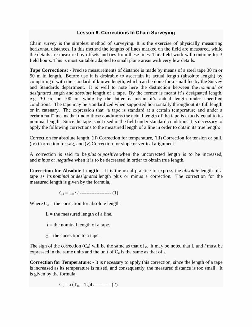
Correction for Sag: - (Fig.1). When a tape is stretched over points of support, it takes the form

of a catenary. In actual practice, however, the catenary curve is

assumed to be a parabola. The correction for sag (or sag correction) is the difference in length

between the arc and the subtending chord (i.e., the difference between the horizontal distance

between supports and the length measured along the curve). It is required only when the tape is

suspended during measurement. Since the effect of the set on the tapes is to make the measured

length too great this correction is always subtractive. It is given by the formula,

Cs = l1 (mgl1)2 / 24P2 = l1(Mg)2 / 24P2 ………………(4)

in which Cs = the sag correction for a single span, in metres.

l1 = the distance between supports in metres.

m = the mass of the tape, in kilograms per metre.

M = Total mass of the tape in kilograms.

P = the applied pull, in newtons (N).

If there are n equal spans per tape length, the sag corrections per tape length is given, by

Cs = nl1(mgl1)2 / 24P2 = l(mgl1)2 / 24P2 = l(mgl)2 / 24n2P2 ………….(4a)

in which l = the length of the tape = nl1, and l1= l/n.

Normal Tension: - The normal tension is a tension at which the effects of pull and sag are

neutralized, i.e. the elongation due to increase in tension is balanced by the shortening due to

sag. It may be obtained by equating the corrections for pull and sag. Thus we have,

(Pn-Po)l1 / AE = l1(mgl1)2 / 24Pn2 or (Pn-Po) Pn

2 = W2AE / 24

~ Pn = 0.204 W √AE / √(Pn-Po) …………………………………………..(5)

in which Pn = the normal tension in newtons (N).

W = the weight of the length of tape between supports in newtons (N).

The value of Pn may be determined by trial

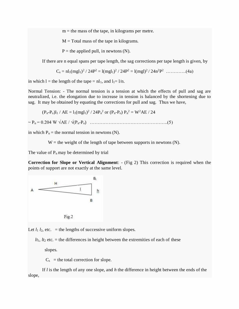
Correction for Slope or Vertical Alignment: - (Fig 2) This correction is required when the

points of support are not exactly at the same level.

Let l1 l2, etc. = the lengths of successive uniform slopes.

lt1, lt2 etc. = the differences in height between the extremities of each of these

slopes.

Cs = the total correction for slope.

If l is the length of any one slope, and h the difference in height between the ends of the

slope,

the slope correction = l - √ l2-h2

= l – l (1 – h2 / 2l2 – h4 / 3l4 – etc..)

=(h2 / 2l + h4 / 3l3 + etc.) = h2 / 2l ------------------------(6)

hence, Cs = (h12 / 2l1 + h2

2 / 2l2 + ….. + hn2 / 2ln) -------------------------------(6a)

When the slopes are of uniform length l we have

Cs = l / 2l (h12 + h2

2 + ……… + hn2) = ∑h2 / 2l -------------------------(6b)

This correction is always subtractive from the measured length. If the slopes are given in terms

of vertical angles (plus or minus angles), the following formula may be used:

The correction for the slope = l – l cos 0 = 2l sin2 0 / 2

= l versin 0 (-ve) --------------------------(7)

in which l = the length of the slope : 0 = the angle of the slope.

Examples on Tape Corrections

Examples 1: - A line was measured with a steel tape which was exactly 30m long at 18oC and found to be 452.343 m. The temperature during measurement was 32oC. Find the true length of the line. Take coefficient of expansion of the

tape per oC=0.0000117.

Temperature correction per tape length = Ct

= α (Tm - To) l

Here l = 30 m: To =18oC; Tm = 32oC;

α = 0.0000117

~ Ct = 0.0000117 (32-18) 30

= 0.004914 m (+ ve)

Hence the length of the tape at 32oC = 30 + Ct

= 30 + 0.004914 = 30.004914 m.

Now true length of a line = L’ / L x its measured length.

L = 30 m: L’ = 30.004914 m; measured length = 452.343 m.

~ True length = 30.004914 / 30 x 452.343 = 452.417 m.

Example 2: - A line was measured with a steel rape which was exactly 30 m at 18oC and a pull of 50 N and the measured length was 459.242 m. Temperature during

measurement was 28oC and the pull applied was 100 N. The tape was uniformly supported

during the measurement. Find the true length of the line if the cross-sectional area of the tape

was 0.02 cm2, the coefficient of expansion

per oC = 0.0000117 and the modulus of elasticity = 21 x 106 N per cm2.

Temperature

Correction per tape length = α ( (Tm – To)L

= 0.0000117 x (28 -18) 30

= 0.00351 m (+ ve)

Sag correction per tape length = 0

Pull correction per tape length = (Pm - Po)L / AE

= (100 – 50)30 / 0.02 x 21 x 106

= 0.00357 m (+ve)

~ Combined correction = 0.00351 + 0.00357 m.

= 0.00708 m

True length of tape = 30.00708 m

True length of the line = 30.00708 / 30 x 459.242

= 459.350 m.

Example 3: - A 50 m tape is suspended between the ends under a pull of

150 N. The mass of the tape is 1.52 kilograms. Find the corrected length of the tape.

Correction for sag = Cs = l1 (Mg)2 / 24 P2

l1 = 50 m; M = 1.52 kilograms; P = 150 N.

~ Cs = 50 x (1.52 x 9.81)2 / 24 x 1502 = 0.0206 m.

~ Corrected length of the tape = l – Cs

= 50 – 0.0206

= 49.9794 m.

Example 4: - The downhill end of the 30 m tape is held 80 cm too low. What is the horizontal

length?

Correction for slope = h2 / 2l

Here h = 0.8 m; l = 30 m

~ The required correction = 0.82 / 2 x 30 = 0.0167 m.

Hence the horizontal length = 30 – 0.0167

= 29.9833 m

Example 5: - A 100 m tape is held 1.5 m out of line. What is the true length?

Correction for incorrect alignment = d2 / 2l ( - ve)

Here d = 1.5 m; l = 100 m.

~ Correction = 1.52 / 2 x 100 = 0.011 m.

~ True length = 100 – 0.011 = 99.989 m.

Lesson 6. Corrections In Chain Surveying

Chain survey is the simplest method of surveying. It is the exercise of physically measuring

horizontal distances. In this method the lengths of lines marked on the field are measured, while

the details are measured by offsets and ties from these lines. This field work will continue for 3

field hours. This is most suitable adapted to small plane areas with very few details.

Tape Corrections: - Precise measurements of distance is made by means of a steel tape 30 m or

50 m in length. Before use it is desirable to ascertain its actual length (absolute length) by

comparing it with the standard of known length, which can be done for a small fee by the Survey

and Standards department. It is well to note here the distinction between the nominal or

designated length and absolute length of a tape. By the former is meant it’s designated length,

e.g. 30 m, or 100 m, while by the latter is meant it’s actual length under specified

conditions. The tape may be standardized when supported horizontally throughout its full length

or in catenary. The expression that “a tape is standard at a certain temperature and under a

certain pull” means that under these conditions the actual length of the tape is exactly equal to its

nominal length. Since the tape is not used in the field under standard conditions it is necessary to

apply the following corrections to the measured length of a line in order to obtain its true length:

Correction for absolute length, (ii) Correction for temperature, (iii) Correction for tension or pull,

(iv) Correction for sag, and (v) Correction for slope or vertical alignment.

A correction is said to be plus or positive when the uncorrected length is to be increased,

and minus or negative when it is to be decreased in order to obtain true length.

Correction for Absolute Length: - It is the usual practice to express the absolute length of a

tape as its nominal or designated length plus or minus a correction. The correction for the

measured length is given by the formula,

Ca = Lc / l ------------------- (1)

Where Ca = the correction for absolute length.

L = the measured length of a line.

l = the nominal length of a tape.

C = the correction to a tape.

The sign of the correction (Ca) will be the same as that of c. it may be noted that L and l must be

expressed in the same units and the unit of Ca is the same as that of c.

Correction for Temperature: - It is necessary to apply this correction, since the length of a tape

is increased as its temperature is raised, and consequently, the measured distance is too small. It

is given by the formula,

Ct = a (Tm – To)L-----------(2)

in which Ct = the correction for temperature, in m.

a = the coefficient of thermal expansion.

Tm = the mean temperature during measurement.

To = the temperature at which the tape is standardized.

L = the measure length in m.

The sign of the correction is plus or minus according as T m is greater or less

than To. The coefficient of expansion for steel varies from 10.6 x 10-6 to 12.2 x 10-6 per degree

centigrade and that for invar from 5.4 x 10-7 to 7.2 x 10-7. If the coefficient of expansion of a

tape is not known, an average value of 11.4 x 10-6 for steel and

6.3 x 10-7 for invar may be assumed. For very precise work, the coefficient of expansion for the

tape in question must be carefully determined.

Correction for Pull (or Tension): - The correction is necessary when the pull used during

measurement is different from that at which the tape is standardized. It is given by the formula,

Cp = (P-Po)L / AE ----------(3)

Where Cp = the correction for pull in metres.

P = the pull applied during measurement, in newtons (N).

Po= the pull under which the tape is standardized in newtons (N).

L = the measured length in metres.

A = the cross-sectional area of the tape, in sq.cm.

E = the modulus of elasticity of steel.

The value of E for steel may be taken as 19.3 to 20.7 x 1010 N/m2 and that for invar 13.8 to 15.2

x 1010 N/m2. For every precise work its value must be ascertained. The sign of the correction is

plus, as the effect of the pull is to increase the length of the tape and consequently, to decrease

the measured length of the line.

Correction for Sag: - (Fig.1). When a tape is stretched over points of support, it takes the form

of a catenary. In actual practice, however, the catenary curve is assumed to be a parabola.

The correction for sag (or sag correction) is the difference in length between the arc and the

subtending chord (i.e., the difference between the horizontal distance between supports and the

length measured along the curve). It is required only when the tape is suspended during

measurement. Since the effect of the set on the tapes is to make the measured length too great

this correction is always subtractive. It is given by the formula,

Cs = l1 (mgl1)2 / 24P2 = l1(Mg)2 / 24P2 ………………(4)

in which Cs = the sag correction for a single span, in metres.

l1 = the distance between supports in metres.

m = the mass of the tape, in kilograms per metre.

M = Total mass of the tape in kilograms.

P = the applied pull, in newtons (N).

If there are n equal spans per tape length, the sag corrections per tape length is given, by

Cs = nl1(mgl1)2 / 24P2 = l(mgl1)2 / 24P2 = l(mgl)2 / 24n2P2 ………….(4a)

in which l = the length of the tape = nl1, and l1= l/n.

Normal Tension: - The normal tension is a tension at which the effects of pull and sag are

neutralized, i.e. the elongation due to increase in tension is balanced by the shortening due to

sag. It may be obtained by equating the corrections for pull and sag. Thus we have,

(Pn-Po)l1 / AE = l1(mgl1)2 / 24Pn2 or (Pn-Po) Pn

2 = W2AE / 24

~ Pn = 0.204 W √AE / √(Pn-Po) …………………………………………..(5)

in which Pn = the normal tension in newtons (N).

W = the weight of the length of tape between supports in newtons (N).

The value of Pn may be determined by trial.

Correction for Slope or Vertical Alignment: - (Fig 2) This correction is required when the

points of support are not exactly at the same level.

Let l1 l2, etc. = the lengths of successive uniform slopes.

lt1, lt2 etc. = the differences in height between the extremities of each of these

slopes.

Cs = the total correction for slope.

If l is the length of any one slope, and h the difference in height between the ends of the

slope,

the slope correction = l - √ l2-h2

= l – l (1 – h2 / 2l2 – h4 / 3l4 – etc..)

=(h2 / 2l + h4 / 3l3 + etc.) = h2 / 2l ------------------------(6)

hence, Cs = (h12 / 2l1 + h2

2 / 2l2 + ….. + hn2 / 2ln) -------------------------------(6a)

When the slopes are of uniform length l we have

Cs = l / 2l (h12 + h2

2 + ……… + hn2) = ∑h2 / 2l -------------------------(6b)

This correction is always subtractive from the measured length. If the slopes are given in terms

of vertical angles (plus or minus angles), the following formula may be used:

The correction for the slope = l – l cos 0 = 2l sin2 0 / 2

= l versin 0 (-ve) --------------------------(7)

in which l = the length of the slope : 0 = the angle of the slope.

Examples on Tape Corrections

Examples 1: - A line was measured with a steel tape which was exactly 30m long at 18oC and

found to be 452.343 m. The temperature during measurement was 32oC. Find the true length of

the line. Take coefficient of expansion of the tape per oC=0.0000117.

Temperature correction per tape length = Ct

= α (Tm - To) l

Here l = 30 m: To =18oC; Tm = 32oC;

α = 0.0000117

~ Ct = 0.0000117 (32-18) 30

= 0.004914 m (+ ve)

Hence the length of the tape at 32oC = 30 + Ct

= 30 + 0.004914 = 30.004914 m.

Now true length of a line = L’ / L x its measured length.

L = 30 m: L’ = 30.004914 m; measured length = 452.343 m.

~ True length = 30.004914 / 30 x 452.343 = 452.417 m.

Example 2: - A line was measured with a steel rape which was exactly 30 m at 18oC and a pull

of 50 N and the measured length was 459.242 m. Temperature during measurement was 28oC

and the pull applied was 100 N. The tape was uniformly supported during the

measurement. Find the true length of the line if the cross-sectional area of the tape was 0.02

cm2, the coefficient of expansion

per oC = 0.0000117 and the modulus of elasticity = 21 x 106 N per cm2.

Temperature

Correction per tape length = α ( (Tm – To)L

= 0.0000117 x (28 -18) 30

= 0.00351 m (+ ve)

Sag correction per tape length = 0

Pull correction per tape length = (Pm - Po)L / AE

= (100 – 50)30 / 0.02 x 21 x 106

= 0.00357 m (+ve)

~ Combined correction = 0.00351 + 0.00357 m.

= 0.00708 m

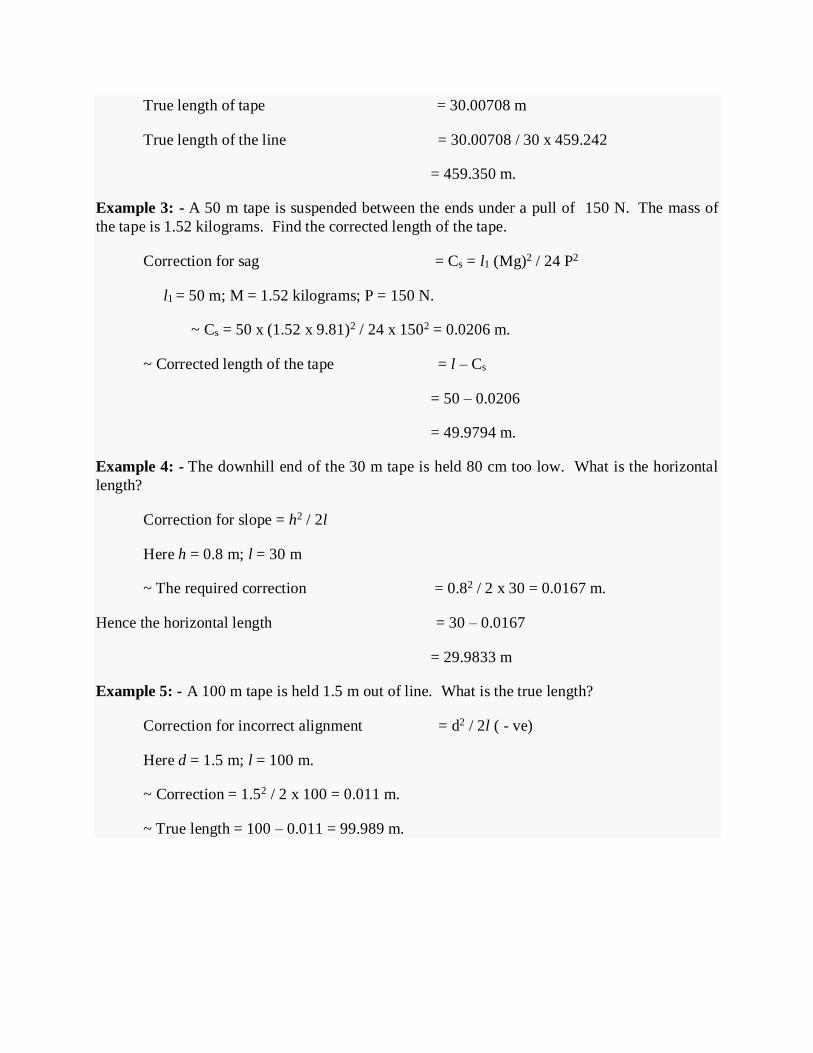
True length of tape = 30.00708 m

True length of the line = 30.00708 / 30 x 459.242

= 459.350 m.

Example 3: - A 50 m tape is suspended between the ends under a pull of 150 N. The mass of

the tape is 1.52 kilograms. Find the corrected length of the tape.

Correction for sag = Cs = l1 (Mg)2 / 24 P2

l1 = 50 m; M = 1.52 kilograms; P = 150 N.

~ Cs = 50 x (1.52 x 9.81)2 / 24 x 1502 = 0.0206 m.

~ Corrected length of the tape = l – Cs

= 50 – 0.0206

= 49.9794 m.

Example 4: - The downhill end of the 30 m tape is held 80 cm too low. What is the horizontal

length?

Correction for slope = h2 / 2l

Here h = 0.8 m; l = 30 m

~ The required correction = 0.82 / 2 x 30 = 0.0167 m.

Hence the horizontal length = 30 – 0.0167

= 29.9833 m

Example 5: - A 100 m tape is held 1.5 m out of line. What is the true length?

Correction for incorrect alignment = d2 / 2l ( - ve)

Here d = 1.5 m; l = 100 m.

~ Correction = 1.52 / 2 x 100 = 0.011 m.

~ True length = 100 – 0.011 = 99.989 m.

Lesson 7. Plane table surveying

Plane Table Surveying

Plane table surveying is a graphical method of surveying in which the field works and the

plotting is done simultaneously. It is particularly adopting in small areas mapping. Plane

table surveying is used for locating the field computation of area of field.

Merits

It is most suitable for preparing small scale map or surveying small area.

It is most rapid method.

Field book is not necessary.

No great skill is required for satisfactory map.

It is particularly suitable for magnetic area where prismatic compass is not reliable.

Contour and irregular object may be represented accurately.

It is less costly.

Demerits

Plane Table Essentially a tropical instruments.

It is not suitable to work in wet climate.

There are several accessories to be carried out and therefore they are likely to be lost.

It is not suitable for accurate work.

Plane Table essentially consists of a Drawing board mounted on tripod stand and Alidade.

1. Drawing board mounted on tripod

A sheet of drawing paper, called plane table sheet is fastened to the board. Board is made up of

well seasoned wood such as teak of size 40x30 to 75x60cm. it had plane and smooth top. It is

mounted on a tripod in manner that it can be leveled. Leveling up of the table is done by shifting

the legs of tripod. Some tripod provided with leveling screw or by ball and socket head for

accurate leveling.

2. Alidade:

Alidade consists of two vertical sight vane fitted at end the end of straightedge. The straight edge

ruler usually made of brass or teak wood graduated beloved edge. One of the sight veins is

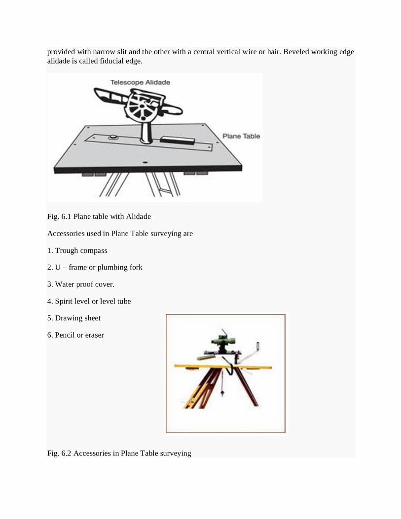
provided with narrow slit and the other with a central vertical wire or hair. Beveled working edge

alidade is called fiducial edge.

Fig. 6.1 Plane table with Alidade

Accessories used in Plane Table surveying are

1. Trough compass

2. U – frame or plumbing fork

3. Water proof cover.

4. Spirit level or level tube

5. Drawing sheet

6. Pencil or eraser

Fig. 6.2 Accessories in Plane Table surveying

Trough compass: The compass is used to mark the direction of the meridian on the paper.

U- frame or Plumbing fork: U frame with a plumb bob used for centering the table.

Water Proof Cover: Water Proof cover protects the sheet from rain.

Spirit level or level tube: A level tube is used to level the plane table.

Drawing sheet: The drawing sheet is fixed on the top of the drawing board.

Pencil and eraser: A pencil is used for constructing lines and eraser is used for erasing lines after

completion of the plan.

Operations involved in Plane Table Surveying

SETTING UP THE PLANE TABLE

The setting up the plane table includes the following three operations.

1. Centering the plane table

2. Leveling the plane table

3. Orientation of plane table

CENTERING THE PLANE TABLE:

The table should be set up at a convenient height for working say about 1m. The legs of tripod

should be spread well apart and firmly fixed in to the ground. The table should be approximately

leveled by tripod legs and judging by the eye. Then the operation of centering is carried out by

means of U-frame and plumb bob. The plane table is exactly placed over the ground station by

U-frame and plumb bob.

LEVELING THE PLANE TABLE:

The process of leveling is carried out with the help of level tube. The bubble of level tube is

brought to center in two directions, which are right angles to each other. This is achieved by

moving legs.

ORIENTING THE TABLE:

The process of keeping the plane table always parallel to the position, which is occupied at the

first station, is known as orientation. When the plane table is oriented, the lines on the board are

parallel to the lines on the ground

Lesson 8. Radiation, Intersection and traversing

Methods of Plane table Surveying

1.Radiation method

2. Intersection method

3. Traversing method

1.RADIATION METHOD

The plane table is set up over only one station from which the whole traverse can be

commanded. It is suitable for survey of small areas.

Procedure:

1) Select a point “O ” so that all points to be located are visible from it.

2) Set up the table at “O”, level it, and do centering.

3) SELECT A POINT “O” on the sheet so that it is exactly over station “O” on

4) Mark the direction of the magnetic meridian

5) Centering the alidade on “O” BISECT the objects of traverse A, B, C and D.

6) Measure the distances OA, OB, OC and OD and plotted to convenient scale to locate a, b, c

and d respectively

7) Join the points a, b, c and d on the paper.

Fig. 8.1 Radiation method

2.INTERSECTION METHOD

In this method the plane table is shifted to a known distance in a particular direction marked on

the ground and the line of sights are drawn to make intersection of the radial lines already drawn

from the first set up of the instrument.

PROCEDURE:

1) Select two points P and Q such that the points (building corners) to be plotted are visible from

their stations.

2) Set the table on P and locate on the sheet.

3) Pivot on P bisect Q draw a ray.

4) Measure the distance PQ and locate Q on the sheet to a convenient scale.

5) Now PQ is known as the base line.

6) Pivot ‘P’ bisects the inaccessible objects A and B (building corners) and draw rays.

7) Shift the table to ‘A’ such that P is over Q and do temporary adjustments.

8) Place the alidade along QP and the rotate the table till P is bisected, clamp table.

9) Pivot on Q bisect the objects A and B and draw rays.

10) The instruction of rays drawn from P and Q will give the points A and B.

11) To check the accuracy measured AB and compare with plotted distance AB.

12) The same procedure is applied for other features of the campus. each point is bisected from

two stations.

Fig. 7.2 Intersection method

3.TRAVERSE METHOD

We can traverse an area with the plane table along the boundry to prepare the map or plan of the

area.

PROCEDURE:

1) Select the traverse stations A,B,C,D,E etc on the ground.

2) Set the table on starting station ‘a’ and perform temporary

adjustments.

3) Mark the magnetic meridian.

4) Locate A on the sheet as ‘a’.

5) Pivot on ‘a’ bisect the next station B and draw a ray

6) Measure the distance AB and locate ‘b’ on the sheet with a suitable scale.

7) Shift the table to next station B, set the table over B, and do temporary adjustments.

8) Place the alidade along ‘ba’ and bisect A for doing orientation of plane table.

9) Pivot on b bisect c draw a ray

10) Measure the distance BC and locate ‘c’ on the sheet with the suitable scale.

11) Report the same procedure at every successive station until the traverse is completed.

NOTE: By using radiation method, intersection and traversing methods we can locate the

points on the paper, which were already on the ground. By using algebraic formulae, we

can calculate the area of the given land.

FORMULAE:

1) Area of a triangle = ½ * base *height

2) Area of a square = side * side

3) Area of a rectangle = length * breadth

4) Area of a trapezium = ½ * (a + b) * h

A, b are the parallel sides. h is the distance between parallel sides.

Fig 7.3 Traversing method

Lesson 9. Levelling- description of level instruments

The art of determining relative altitudes of points on the surface of the earth of beneath the

surface of earth is called LEVELLING.

For execution of Engineering Projects it is very necessary to determine elevations of different

points along the alignment of proposed project.

Other applications are :

i) Taking rail levels existing before track renewals to finalise final rail level profile including

vertical curves.

ii) Initial ground levels for earthwork calculations.

iii) Levels for measurement of earthwork.

iv) Measurement of ballast etc.

Terms used in Levelling –

a) DATUM – or Datum plane is an arbitrarily assumed level surface or line with reference to

which level of other line or surface are calculated.

b) REDUCED LEVEL (RL) – Height or depth of a point above or below the assumed datum is

called Reduced level.

c) BENCH MARK – (BM) – B.M. is a fixed reference point of known elevation. It may be of

the following types.

i) GTS Bench mark (Geodetic Triangulation Survey) :

These Bench marks are established by national agency like Survey of India. They are

established with highest precision. Their position and elevation above MSL is given in a special

catalogue known as GTS Maps ( 100 km. interval).

ii) Permanent Bench Mark : They are fixed points of reference establish with reference to GTS

Bench mark (10 km. interval).

iii) Arbitrary Bench mark : These are reference points whose elevations are arbitrarily

assumed. In most of Engineering projects, the difference in elevation is more important than

their reduced levels with reference to MSL as given in a special catalogue known as GTS Maps (

100 Km. interval).

d) Mean Sea Level (M.S.L.) : M.S.L. is obtained by making hourly observations of the tides at

any place over a period of 19 years. MSL adopted by Survey of India is now Bombay which was

Karachi earlier.

e) Level Surface : The surface which is parallel to the mean sphereoidal surface of the earth is

known as level surface.

f) Line of Collimation : It is the line joining the intersection of the cross hair and the optical

center of the objective and its extensions, it is also called line of sight or collimation.

g) Height of Instrument (HI) : The elevation of the line of sight with respect to assumed datum

is known as height of Instrument(HI).

h) Back sight : (B.S.) - The first sight taken on a levelling staff held at a point of known

elevation. B.S. enables the surveyor to obtain HI +sight i.e. Height of Instrument or line of sight.

i) Fore Sight : (F.S.) – It is the last staff reading taken from a setting of the level. It is also

termed as minus sight.

Fore sight is the sight taken on a levelling staff held at a point of unknown elevation to ascertain

the amount by which the point is above or below the line of sight. This is also called minus sight

as the foresight reading is always subtracted from height of Instrument.

j) Change Point (CP) : The point on which both the foresight and back sight are taken during the

operation of levelling is called change point.

k) Intermediate Sight (IS) :

The foresight taken on a levelling staff held at a point between two turning points, to determine

the elevation of that point, is known as intermediate sight.

It may be noted that for one setting of a level, there will be only one back sight and one foresight

but there can be any number of intermediate sights.

Type of Levelling Equipments:

i) Dumpy level

ii) Tilting level

iii) Automatic level

iv) Digital Auto level

Dumpy level : It is simple compact and stable. The telescope is rigidly fixed to its support

therefore cannot be rotated about its longitudinal axis. A long bubble tube is attached to the top

of telescope. Dumpy literally means short and thick.

Tilting level : It consists of a telescope attached with a level tube which can be tilted within few

degrees in vertical plane by a tilting screw. The main peculiarity of this level is that the vertical

axis need not be truly vertical, since the line of collimation is not perpendicular to it. The line of

collimation, is, however, made horizontal for each pointing of telescope by means of tilting

screw. It is mainly designed for precise levelling work.

The Automatic level : Also termed as self aligning level. The fundamental difference between

automatic and the classic spirit level is that in the former the line of sight is no longer levelled

manually using a tubular spirit level, but is levelled automatically within a certain tilt

range. This is achieved by compensator in the telescope.

DUMPY LEVEL

It is simple compact and stable. The telescope is rigidly fixed to its support therefore cannot be

rotated about its longitudinal axis. A long bubble tube is attached to the top of

telescope. Dumpy literally means short and thick.

Fig 9.1 Dumpy level

Fig 9.2 Parts of Dumpy level

The different parts of levelling instrument are,

(a)Telescope

(b) Eye-piece

(c) focussing knob

(d) level tube

(e) cross bubble

(f) foot screws

(g) levelling head

(h) diaphragm

(i) ray shade

Basic components of level :

1. Telescope – to provide a line of sight

2. Level Tube – to make line of sight horizontal

3. Levelling head – to bring the bubble of tube level at the centre of its run.

4. Tripod – to support the above three parts of the level.

TELESCOPE : Telescope is an optical instrument used for magnifying and viewing the images

of distant objects. It consists of two lenses. The lens fitted near the eye is called the eye piece

and the other fitted at the end near to the object is called the objective lens. The objective

provides a real inverted image infront of the eye piece at a distance lesser than its focal distance.

Two essential conditions are involved. :

i) The real image of the object, must be formed.

ii) the plane of image must coincide with that of cross hairs.

Focusing of Telescope : The operation of obtaining a clear image of the object in the plane of

cross hairs is known as focusing.

1. Diaphram : A frame carrying cross hairs usually made of either silk thread or platinum wire

and placed at the plane at which vertical image of the object is formed by the objective. Vertical

hair of the diaphram enables the surveyor to check the verticality of levelling staff whereas

horizontal hairs are used to read the staff graduations.

2. Level Tube : Also known as Bubble Tube consists of a glass tube placed in a brass tube

which is sealed with plaster of paris. The whole of the interior surface or the upper half is

accurately ground so that its longitudinal section, is an arc of a circle. Level tube is filled with

either or alcohol, the remaining space is occupied by an air bubble. The centre of air bubble

always rest at the highest point of the tube. Outer surface of the bubble tube is graduated in both

the directions from the centre. The line tangential to the circular are at its highest point i.e. the

middle of tube is called the axis of bubble tube. When the bubble is central the axis of bubble

becomes Horizontal. The level tube is attached on the top of Telescope by means of capstan

headed nuts.

3. Levelling head : Levelling head generally consists of two parallel plates with 3 foot

screws. Upper plate is known as Tribrach and lower plate is trivet which can be screwed on to

the tripod. Levelling head has to perform three distinct functions :

i) to support the telescope

ii) to attach the level to the tripod

iii) to provide a means for level (foot screws)

Adjustments of level :

(i) Temporarily Adjustments – adjustments which are made for every setting of a level.

(ii) Permanent adjustments- required if some error is there in instrument.

(i) Temporary Adjustments : includes

a) setting up the level

b) levelling up

c) elimination of parallax

a) Setting up the level : This operation includes fixing the instrument on the tripod and also

approximate levelling by leg adjustment.

b) Levelling up : Accurate levelling is done with the help of foot screws and by using plate

levels. The object of levelling up the instrument is to make its vertical axis truly vertical.

c) Elimination of parallax : If the image formed by the objective does not lie in the plane of the

cross hairs, there will be a shift in the image due to shift of the eye. Such displacement of image

is termed as parallax. Parallax is removed in two stages.

1) Focusing the eye for distinct vision of cross hairs.

2) Focusing the objective so that image is formed in the plane of cross hairs.

Levelling staff

It is an important accessory used with levelling instrument at the time of conducting levelling

survey. Reading is taken on the levelling staff held properly at the point concerned by viewing

through the telescope of the levelling instrument. Usually 4 m levelling staff may be used of

folding type or telescopic type. Aluminium levelling staff foldable at every metre length has also

came to the market. The levelling staff consists of three pieces. The topmost one slides into the

middle one and the middle portion slides into the bottom one. When the staff is fully pulled, it

will read exactly 40 decimeters (4m) from the bottom shoe.

Graduation in levelling staff:

Every metre length is divided into 200 divisions.

The divisions are painted in black and white alternately of thickness 5 mm each.

The graduation figures are marked at every decimeter length.

The number indicating metre is in red and the decimeter number is in black.

Thus, a graduation figure of 24 indicates 2 metres and 4 decimeters.

The graduation are made continuously one above the other in the same line.

The division lines should be parallel to the base of the bottom shoe and perpendicular to

the length of the staff.

The edges of the division lines should be straight sharply defined.

They should be clear and made distinctly visible by properly contrasting.

The graduation colour paints used should not crack or blister when exposed to adverse or

atmospheric conditions.

Lesson 10. Simple levelling and fly levelling methods

The art of determining relative altitudes of points on the surface of the earth of beneath the

surface of earth is called LEVELLING.

For execution of Engineering Projects it is very necessary to determine elevations of different

points along the alignment of proposed project.

Other applications are :

i) Taking rail levels existing before track renewals to finalise final rail level profile including

vertical curves.

ii) Initial ground levels for earthwork calculations.

iii) Levels for measurement of earthwork.

iv) Measurement of ballast etc.

Adjustments of level :

(i) Temporarily Adjustments – adjustments which are made for every setting of a level.

(ii) Permanent adjustments- required if some error is there in instrument.

(i) Temporary Adjustments : includes

a) setting up the level

b) levelling up

c) elimination of parallax

a) Setting up the level : This operation includes fixing the instrument on the tripod and also

approximate levelling by leg adjustment.

b) Levelling up : Accurate levelling is done with the help of foot screws and by using plate

levels. The object of levelling up the instrument is to make its vertical axis truly vertical.

c) Elimination of parallax : If the image formed by the objective does not lie in the plane of the

cross hairs, there will be a shift in the image due to shift of the eye. Such displacement of image

is termed as parallax. Parallax is removed in two stages.

1) Focusing the eye for distinct vision of cross hairs.

2) Focusing the objective so that image is formed in the plane of cross hairs.

Principles of levelling :

a) Simple levelling : The operation of levelling for determining the difference in elevation, if

not too great between two points visible from single position of the level is known as simple

levelling.

Fig 10.1 Simple levelling

Procedure to be followed

1. Level the instrument correctly.

2. Direct the telescope towards the staff held

3. Take the reading of Central, horizontal hair of the diaphram, where it appears to cut the

staff ensuring that the bubble is central.

4. Send the staff to next point

5. Direct the telescope towards C and focus it again

6. Check up the bubble if central, if not bring it to the Central position by the foot screw

nearest to the telescope.

7. Take the reading of Central Horizontal cross hair.

b)Differential levelling or fly levelling :

Any number of change points are established as required during levelling. This method is known

as fly levelling.

It is adopted to find the difference in level between two points, when

(i) The two points are too far away

(ii) the difference in level between two points is large

(iii) there are no obstructions in between the two points concerned.

This method is used in order to find the difference in elevation between two points.

i) If they are too far apart

ii) if the difference in elevation between them is too great.

iii) If there are obstacles intervening. In such case it is necessary to set up the level in several

positions and to work in series of stages.

The difference of level of the points A&B is equal to the algebraic sum of these difference

between the sum of back sights and sum of the fore sights i.e. Σ BS - Σ FS.

The elevation of change point = Elevation of P + Back sight at P – Fore

sight at change point (C.P)

= 100.00+1.60-1.10 = 100.50 m

The second height of the instrument = The elevation of change point+

Back Sight at change point

= 100.50+1.25 = 101.75 m

The elevation of Q = The second height of instrument –

foresight at Q

= 101.75 – 1.81 = 99.94 m

RISE AND FALL METHOD

The staff readings of the points observed from the same setting of the instrument are

compared.

It is found whether a point is above or below the preceding point.

If the point is above, the staff reading will be less than the preceding point. The

difference between the staff readings is called rise.

If the point is below the preceding point, the staff reading will be greater than that at the

preceding point. The difference between the staff readings is termed fall.

The difference between the staff readings at P and Q = 2.10 – 1.80 = 0.30 (rise)

Hence, level of Q = Elevation of P + Rise = 100.00+0.30 = 100.30 m

Back

sight

Intermediate

station

Fore

sight Rise Fall

Reduced

Level Remarks

1.245

100.00 BM

2.100

0.855 99.145

2.425

0.810 1.290

100.435 STATION

A

0.480 1.945

102.380

STATION

B

∑BS

∑FS ∑RISE ∑FALL

3.670 1.290 3.235 0.855

Arithmetical Check of Rise and Fall method

∑ B.S - ∑F.S = ∑Rise - ∑ Fall = Last R.L – First R.L.

3.670 – 1.290 = 3.235 – 0.855 = 102.380 – 100.00

2.380 = 2.380 = 2.380

Height of collimation or Height of instrument method

In this method, the height of the instrument is established for each setting of the instrument and

the reduced level of the new point is arrived by detecting the fore sight reading of that point.

Lesson 11. Contours- Introduction

The art of determining relative altitudes of points on the surface of the earth of beneath the

surface of earth is called LEVELLING.

A contour is defined as an imaginary line of constant elevation on the ground surface. It can also

be defined as the line of intersection of a level surface with the ground surface. For example, the

line of intersection of the water surface of a still lake or pond with the surrounding ground

represents a contour line.

Definition:

A line joining points of equal elevations is called a contour line. It facilitates depiction of the

relief of terrain in a two dimensional plan or map.

Characteristics of contour:

The principal characteristics of contour lines which help in plotting or reading a contour map are

as follows:

1. The variation of vertical distance between any two contour lines is assumed to be

uniform.

2. The horizontal distance between any two contour lines indicates the amount of slope and

varies inversely on the amount of slope. Thus, contours are spaced equally for uniform

slope

3. The steepest slope of terrain at any point on a contour is represented along the normal of

the contour at that point. They are perpendicular to ridge and valley lines where they

cross such lines.

4. Contours do not pass through permanent structures such as buildings.

5. Contours of different elevations cannot cross each other (caves and overhanging cliffs are

the exceptions).

6. Contours of different elevations cannot unite to form one contour (vertical cliff is an

exception).

7. Contour lines cannot begin or end on the plan.

8. A contour line must close itself but need not be necessarily within the limits of the map.

9. A closed contour line on a map represents either depression or hill . A set of ring contours

with higher values inside, depicts a hill whereas the lower value inside, depicts a

depression (without an outlet).

10. Contours deflect uphill at valley lines and downhill at ridge lines. Contour lines in U-

shape cross a ridge and in V-shape cross a valley at right angles. The concavity in

contour lines is towards higher ground in the case of ridge and towards lower ground in

the case of valley .

11. Contours do not have sharp turnings.

Contour Interval:

The vertical distance between any two consecutive contours is known as a contour interval.

For example, if the various consecutive contours are 100m, 98m,96 m etc., then the contour

interval is 2m. This interval depends upon,

The nature of the ground

The scale of the map and

The purpose of survey

Contour intervals for flat country are generally small, eg. 0.25m, 0.5m, 0.75 m etc. For a steep

slope in hilly area is greater, eg. 5m, 10m, 15 m etc.

Again ,for a small-scale map, the interval may be of 1m,2m,3m etc. and for large scale map,it

may be of 0.25m,0.50m,0.75m etc.

It should be remembered that the contour interval for a particular map is constant.

Contouring:

The process of locating these contour lines on the surface of the earth is known as contouring.

Methods of contouring:

The method of establishing / plotting contours in a plan or map is known as contouring. It

requires planimetric position of the points and drawing of contours from elevations of the plotted

points. Contouring involves providing of vertical control for location of points on the contours

and horizontal control for planimetric plotting of points. Thus, contouring depends upon the

instruments used (to determine the horizontal as well as vertical position of points). In general,

the field methods of contouring may be divided into two classes:

1. Direct methods

2. Indirect methods

Direct Method:

In the direct method, the contour to be plotted is actually traced on the ground. Points which

happen to fall on a desired contour are only surveyed, plotted and finally joined to obtain the

particular contour. This method is slow and tedious and thus used for large scale maps, small

contour interval and at high degree of precision.

Vertical control :

In this method, a benchmark is required in the project area. The level is set up on any

commanding position and back sight is taken on the bench mark. Let the back sight reading on

the bench mark be 1.485 m. If the reduced level of the bench mark is 100 m, the height of

instrument would be 100 + 1.485 = 101.485 m.

To locate the contour of 100.5 m value, the staff man is directed to occupy the position on the

ground where the staff reading is 101.485 -100.500 = 0.985 m. Mark all such positions on the

ground where the staff reading would be 0.985 m by inserting pegs. Similarly locate the points

where the staff reading would be 101.485 -101 = 0.485 m for 101m contour.

The contour of 101.5 m cannot be set from this setting of the instrument because the height of

instrument for this setting of the instrument is only 101.485 m. Therefore, locating contours of

higher value, the instrument has to be shifted to some other suitable position.

Establish a forward station on a firm ground and take fore sight on it. This point acts as a point of

known elevation, for shifting the position of the instrument to another position, from where the

work proceeds in the similar manner till the entire area is contoured.

Horizontal control :

The horizontal control is generally provided by method of plane table surveying or locating the

positions of points.

Indirect method of contouring:

In this method, the spot levels of selected guide points are taken with a level and their levels are

computed. The horizontal positions of these points are measured or computed and the points are

plotted on the plan. The contours are then drawn by a process called interpolation of contours

from the levels of the guide points. The following are the indirect methods are commonly used

for locating contours.

1. Squares or Grid method

2. Cross section method

Square or grid method:

In this method, the area to be surveyed is divided into a grid or series of squares. The grid size

may vary from 5 m x 5 m to 25 m x 25 m depending upon the nature of the terrain, the contour

interval required and the scale of the map desired. Also, the grids may not be of the same size

throughout but may vary depending upon the requirement and field conditions. The grid corners

are marked on the ground and spot levels of these comers are determined by leveling. The grid is

plotted to the scale of the map and the spot levels of the grid corners are entered. The contours of

desired values are then located by interpolation. Special care should be taken to give the spot

levels to the salient features of the ground such as hilltops, deepest points of the depressions, and

their measurements from respective corners of the grids, for correct depiction of the features. The

method is used for large scale mapping and at average precision.

Cross section method:

In these sections, a base line, centre line or profile line is considered. Cross sections are taken

perpendicular to this line at regular intervals. After this points are marked along the cross

sections at regular intervals. A temporary bench mark is set up near the site. Staff readings are

taken along the base line and the cross sections. The readings are entered in the level book the

base line and the cross sections should also be mentioned. The RL of each of the points

calculated. Then the base line and cross sections are plotted to a suitable scale. Subsequently

the RLs of the respective points are noted on the map, after which the required contour line is

drawn by interpolation

This method is suitable for route survey, when cross sections are taken transverse to the

longitudinal section.

Method of interpolation of contours:

The process of locating the contours proportionately between the plotted points is termed

interpolation. Interpolation may be done by:

1. Arithmetical calculation

2. The graphical method

By arithmetical calculation

Let A and B be two corners of the squares. The RL of A is 98.75 m, and that of B 100.75 m. the

horizontal distance between A and B is 10m.

Horizontal distance between A and B = 10m

Vertical difference A and B = 100.75-98.75=2m

Let a contour of 99.00 m be required. Then,

Difference of level between A and 99.00m contour = 99.00-98.75=0.25m

Therefore, distance of 99.00 m contour line form A= 10/2 *0.25=1.25m

This calculated distance is plotted to the same scale in which the skeleton was plotted to obtain a

point of RL of 99.00 m.

Similarly, the other points can be located.

By graphical method

On a sheet of tracing paper, a line AB is drawn and divided into equal parts. AB is bisected at C

and a perpendicular is drawn at this point. A point O is selected on this perpendicular line and

then radial lines are drawn from O to the divisions on AB. After this lines 1-1, 2-2, 3-3….are

drawn parallel to AB. These lines serve as guide lines. Boundary line and every fifth the line is

marked with a thick or red line.

Suppose we have to interpolate a 2m contour between two points a and b of RLs 92.5 and

100.75m.

Let us consider the lowest radial line OB to represent an RL of 90.00. So, every fifth line will

represent 95,100,105, etc. The tracing paper is moved over the plan until ‘a’ lies at 92.5 and ‘b’

at 100.25. Line ‘ab’ should be parallel to AB. Now the points 94, 96, 98,100 are picked through

to obtain the positions of the required contours.

Method of interpolation of contours:

The process of locating the contours proportionately between the plotted points is termed

interpolation. Interpolation may be done by:

1. Arithmetical calculation

2. The graphical method

By arithmetical calculation

Let A and B be two corners of the squares. The RL of A is 98.75 m, and that of B 100.75 m. the

horizontal distance between A and B is 10m.

Horizontal distance between A and B = 10m

Vertical difference A and B = 100.75-98.75=2m

Let a contour of 99.00 m be required. Then,

Difference of level between A and 99.00m contour = 99.00-98.75=0.25m

Therefore, distance of 99.00 m contour line form A= 10/2 *0.25=1.25m

This calculated distance is plotted to the same scale in which the skeleton was plotted to obtain a

point of RL of 99.00 m.

Similarly, the other points can be located.

By graphical method

On a sheet of tracing paper, a line AB is drawn and divided into equal parts. AB is bisected at C

and a perpendicular is drawn at this point. A point O is selected on this perpendicular line and

then radial lines are drawn from O to the divisions on AB. After this lines 1-1, 2-2, 3-3….are

drawn parallel to AB. These lines serve as guide lines. Boundary line and every fifth the line is

marked with a thick or red line.

Suppose we have to interpolate a 2m contour between two points a and b of RLs 92.5 and

100.75m.

Let us consider the lowest radial line OB to represent an RL of 90.00. So, every fifth line will

represent 95,100,105, etc. The tracing paper is moved over the plan until ‘a’ lies at 92.5 and ‘b’

at 100.25. Line ‘ab’ should be parallel to AB. Now the points 94, 96, 98,100 are picked through

to obtain the positions of the required contours.

Lesson 12. Methods of grid levelling

The art of determining relative altitudes of points on the surface of the earth of beneath the

surface of earth is called LEVELLING.

A contour is defined as an imaginary line of constant elevation on the ground surface. It can also

be defined as the line of intersection of a level surface with the ground surface. For example, the

line of intersection of the water surface of a still lake or pond with the surrounding ground

represents a contour line.

To determine the positions of the contours on a plan the leveling methods are used to find the

relative positions of points on the surface of the ground with reference to certain benchmarks at

regular intervals. This technique of making observations and plotting on a plan is called as grid

leveling.

Contour Interval:

The vertical distance between any two consecutive contours is known as a contour interval. For

example, if the various consecutive contours are 100m, 98m, 96 m etc., then the contour

interval is 2m. This interval depends upon,

The nature of the ground

The scale of the map and

The purpose of survey

Contour intervals for flat country are generally small, eg. 0.25m, 0.5m, 0.75 m etc. For a steep

slope in hilly area is greater, eg. 5m, 10m, 15 m etc.

Again ,for a small-scale map, the interval may be of 1m,2m,3m etc. and for large scale map,it

may be of 0.25m,0.50m,0.75m etc.

It should be remembered that the contour interval for a particular map is constant.

Contouring:

The process of locating these contour lines on the surface of the earth is known as contouring.

Methods of contouring:

The method of establishing / plotting contours in a plan or map is known as contouring. It

requires planimetric position of the points and drawing of contours from elevations of the plotted

points. Contouring involves providing of vertical control for location of points on the contours

and horizontal control for planimetric plotting of points. Thus, contouring depends upon the

instruments used (to determine the horizontal as well as vertical position of points). In general,

the field methods of contouring may be divided into two classes:

1. Direct methods

2. Indirect methods

Direct Method:

In the direct method, the contour to be plotted is actually traced on the ground. Points which

happen to fall on a desired contour are only surveyed, plotted and finally joined to obtain the

particular contour. This method is slow and tedious and thus used for large scale maps, small

contour interval and at high degree of precision.

Vertical control :

In this method, a benchmark is required in the project area. The level is set up on any

commanding position and back sight is taken on the bench mark. Let the back sight reading on

the bench mark be 1.485 m. If the reduced level of the bench mark is 100 m, the height of

instrument would be 100 + 1.485 = 101.485 m.

To locate the contour of 100.5 m value, the staff man is directed to occupy the position on the

ground where the staff reading is 101.485 -100.500 = 0.985 m. Mark all such positions on the

ground where the staff reading would be 0.985 m by inserting pegs. Similarly locate the points

where the staff reading would be 101.485 -101 = 0.485 m for 101m contour.

The contour of 101.5 m cannot be set from this setting of the instrument because the height of

instrument for this setting of the instrument is only 101.485 m. Therefore, locating contours of

higher value, the instrument has to be shifted to some other suitable position.

Establish a forward station on a firm ground and take fore sight on it. This point acts as a point of

known elevation, for shifting the position of the instrument to another position, from where the

work proceeds in the similar manner till the entire area is contoured.

Horizontal control :

The horizontal control is generally provided by method of plane table surveying or locating the

positions of points.

Indirect method of contouring:

In this method, the spot levels of selected guide points are taken with a level and their levels are

computed. The horizontal positions of these points are measured or computed and the points are

plotted on the plan. The contours are then drawn by a process called interpolation of contours

from the levels of the guide points. The following are the indirect methods are commonly used

for locating contours.

1. Squares or Grid method

2. Cross section method

Square or grid method:

In this method, the area to be surveyed is divided into a grid or series of squares. The grid size

may vary from 5 m x 5 m to 25 m x 25 m depending upon the nature of the terrain, the contour

interval required and the scale of the map desired. Also, the grids may not be of the same size

throughout but may vary depending upon the requirement and field conditions. The grid corners

are marked on the ground and spot levels of these comers are determined by leveling. The grid is

plotted to the scale of the map and the spot levels of the grid corners are entered. The contours of

desired values are then located by interpolation. Special care should be taken to give the spot

levels to the salient features of the ground such as hilltops, deepest points of the depressions, and

their measurements from respective corners of the grids, for correct depiction of the features. The

method is used for large scale mapping and at average precision.

Cross section method:

In these sections, a base line, centre line or profile line is considered. Cross sections are taken

perpendicular to this line at regular intervals. After this points are marked along the cross

sections at regular intervals. A temporary bench mark is set up near the site. Staff readings are

taken along the base line and the cross sections. The readings are entered in the level book the

base line and the cross sections should also be mentioned. The RL of each of the points

calculated. Then the base line and cross sections are plotted to a suitable scale. Subsequently

the RLs of the respective points are noted on the map, after which the required contour line is

drawn by interpolation

This method is suitable for route survey, when cross sections are taken transverse to the

longitudinal section.

Lesson 13. Contours- Map preparation

The art of determining relative altitudes of points on the surface of the earth of beneath the

surface of earth is called LEVELLING.

A contour is defined as an imaginary line of constant elevation on the ground surface. It can also

be defined as the line of intersection of a level surface with the ground surface. For example, the

line of intersection of the water surface of a still lake or pond with the surrounding ground

represents a contour line.

Indirect method of contouring:

In this method, the spot levels of selected guide points are taken with a level and their levels are

computed. The horizontal positions of these points are measured or computed and the points are

plotted on the plan. The contours are then drawn by a process called interpolation of contours

from the levels of the guide points. The following are the indirect methods are commonly used

for locating contours.

1. Squares or Grid method

2. Cross section method

Square or grid method:

In this method, the area to be surveyed is divided into a grid or series of squares. The grid size

may vary from 5 m x 5 m to 25 m x 25 m depending upon the nature of the terrain, the contour

interval required and the scale of the map desired. Also, the grids may not be of the same size

throughout but may vary depending upon the requirement and field conditions. The grid corners

are marked on the ground and spot levels of these comers are determined by leveling. The grid is

plotted to the scale of the map and the spot levels of the grid corners are entered. The contours of

desired values are then located by interpolation. Special care should be taken to give the spot

levels to the salient features of the ground such as hilltops, deepest points of the depressions, and

their measurements from respective corners of the grids, for correct depiction of the features. The

method is used for large scale mapping and at average precision.

Cross section method:

In these sections, a base line, centre line or profile line is considered. Cross sections are taken

perpendicular to this line at regular intervals. After this points are marked along the cross

sections at regular intervals. A temporary bench mark is set up near the site. Staff readings are

taken along the base line and the cross sections. The readings are entered in the level book the

base line and the cross sections should also be mentioned. The RL of each of the points

calculated. Then the base line and cross sections are plotted to a suitable scale. Subsequently

the RLs of the respective points are noted on the map, after which the required contour line is

drawn by interpolation

This method is suitable for route survey, when cross sections are taken transverse to the

longitudinal section.

Method of interpolation of contours:

The process of locating the contours proportionately between the plotted points is termed

interpolation. Interpolation may be done by:

1. Arithmetical calculation

2. The graphical method

By arithmetical calculation

Let A and B be two corners of the squares. The RL of A is 98.75 m, and that of B 100.75 m. the

horizontal distance between A and B is 10m.

Horizontal distance between A and B = 10m

Vertical difference A and B = 100.75-98.75=2m

Let a contour of 99.00 m be required. Then,

Difference of level between A and 99.00m contour = 99.00-98.75=0.25m

Therefore, distance of 99.00 m contour line form A= 10/2 *0.25=1.25m

This calculated distance is plotted to the same scale in which the skeleton was plotted to obtain a

point of RL of 99.00 m.

Similarly, the other points can be located.

By graphical method

On a sheet of tracing paper, a line AB is drawn and divided into equal parts. AB is bisected at C

and a perpendicular is drawn at this point. A point O is selected on this perpendicular line and

then radial lines are drawn from O to the divisions on AB. After this lines 1-1, 2-2, 3-3….are

drawn parallel to AB. These lines serve as guide lines. Boundary line and every fifth the line is

marked with a thick or red line.

Suppose we have to interpolate a 2m contour between two points a and b of RLs 92.5 and

100.75m.

Let us consider the lowest radial line OB to represent an RL of 90.00. So, every fifth line will

represent 95,100,105, etc. The tracing paper is moved over the plan until ‘a’ lies at 92.5 and ‘b’

at 100.25. Line ‘ab’ should be parallel to AB. Now the points 94, 96, 98,100 are picked through

to obtain the positions of the required contours.

Method of interpolation of contours:

The process of locating the contours proportionately between the plotted points is termed

interpolation. Interpolation may be done by:

1. Arithmetical calculation

2. The graphical method

By arithmetical calculation

Let A and B be two corners of the squares. The RL of A is 98.75 m, and that of B 100.75 m. the

horizontal distance between A and B is 10m.

Horizontal distance between A and B = 10m

Vertical difference A and B = 100.75-98.75=2m

Let a contour of 99.00 m be required. Then,

Difference of level between A and 99.00m contour = 99.00-98.75=0.25m

Therefore, distance of 99.00 m contour line form A= 10/2 *0.25=1.25m

This calculated distance is plotted to the same scale in which the skeleton was plotted to obtain a

point of RL of 99.00 m.

Similarly, the other points can be located.

By graphical method

On a sheet of tracing paper, a line AB is drawn and divided into equal parts. AB is bisected at C

and a perpendicular is drawn at this point. A point O is selected on this perpendicular line and

then radial lines are drawn from O to the divisions on AB. After this lines 1-1, 2-2, 3-3….are

drawn parallel to AB. These lines serve as guide lines. Boundary line and every fifth the line is

marked with a thick or red line.

Suppose we have to interpolate a 2m contour between two points a and b of RLs 92.5 and

100.75m.

Let us consider the lowest radial line OB to represent an RL of 90.00. So, every fifth line will

represent 95,100,105, etc. The tracing paper is moved over the plan until ‘a’ lies at 92.5 and ‘b’

at 100.25. Line ‘ab’ should be parallel to AB. Now the points 94, 96, 98,100 are picked through

to obtain the positions of the required contours.

LESSON 14. Computation of area and volume

The main objective of the surveying is to compute the areas and volumes.

Generally, the lands will be of irregular shaped polygons.

There are formulae readily available for regular polygons like, triangle, rectangle, square and

other polygons.

But for determining the areas of irregular polygons, different methods are used.

Earthwork computation is involved in the excavation of channels, digging of trenches for laying

underground pipelines, formation of bunds, earthen embankments, digging farm ponds, land

levelling and smoothening. In most of the computation the cross sectional areas at different

interval along the length of the channels and embankments are first calculated and the volume of

the prismoids are obtained between successive cross section either by trapezoidal or prismoidal

formula.

Calculation of area is carried out by any one of the following methods:

a) Mid-ordinate method

b) Average ordinate method

c) Trapezoidal rule

d) Simpson’s rule

The mid-ordinate rule

Consider figure.

Let O1, O2, O3, O4……….On= ordinates at equal intervals

l=length of base line

d= common distance between ordinates

h1,h2,……..hn=mid-ordinates

Area = common distance* sum of mid-ordinates

Average ordinate method

Let O1, O2, …..On=ordinates or offsets at regular intervals

l= length of base line

n= number of divisions

n+1= number of ordinates

THE TRAPEZOIDAL RULE

While applying the trapezoidal rule, boundaries between the ends of ordinates are assumed to be

straight. Thus the areas enclosed between the base line and the irregular boundary line are

considered as trapezoids.

Let O1, O2, …..On=ordinate at equal intervals, and d= common distance between two ordinates

Total area=d/2{ O1+2O2+2O3+…….+2On-1+On}

Thus the trapezoidal rule may be stated as follows:

To the sum of the first and last ordinate, twice the sum of intermediate ordinates is added. This

total sum is multiplied by the common distance. Half of this product is the required area.

Limitation: There is no limitation for this rule. This rule can be applied for any number of

ordinates

SIMPSON’S RULE

In this rule, the boundaries between the ends of ordinates are assumed to form an arc of parabola.

Hence simpson’s rule is some times called as parabolic rule. Refer to figure:

Let

O1, O2, O3= three consecutive ordinates

d= common distance between the ordinates

area AFeDC= area of trapezium AFDC+ area of segment FeDEF

Here,

Area of segment= 2/3* area of parallelogram FfdD

= 2/3* eE*2d

= 2/3 *{ O2- O1+O3 /2 }*2d

So, the area between the first two divisions,

= d/3(O1+4O2+O3)

Similarly, the area of next two divisions

∆2 = d/3(O1+4O2+O3) and so on

Total area = d/3[O1+On+4(O2+O4+……) + 2(O3+O5)]

Thus the rule may be stated as the follows

To the sum of the first and the last ordinate, four times the sum of even ordinates and twice the

sum of the remaining odd ordinates are added. This total sum is multiplied by the common

distance. One third of this product is the required area.

Limitation: This rule is applicable only when the number divisions is even i.e. the number of

ordinates is odd.

The trapezoidal rule may be compared in the following manner:

Trapezoidal rule Simpson’s rule

1. The boundary between the ordinates is

considered to be straight

1. There is no limitation. It can be applied for

any number of ordinates

1. It gives an approximate result

The boundary between the ordinates is considered

to be an arc of a parabola

To apply this rule, the number of ordinates must be

odd

It gives a more accurate result.

Note: sometimes one or both the end of the ordinates may be zero. However they must be taken

into account while applying these rules.

Worked- out problems

Problem 1: The following offsets were taken from a chain line to an irregular boundary line at

an interval of 10 m:

0, 2.50, 3.50, 5.00, 4.60, 3.20, 0 m

Compute the area between the chain line, the irregular boundary line and the end of offsets by:

a) mid ordinate rule

b) the average –ordinate rule

c) the trapezoidal rule

d) Simpson’s rule

Solution: (Refer fig)

Mid-ordinate rule:

Required area= 10(1.25+3.00+4.25+3.90+1.60)

= 10*18.80=188 m2

By average-ordinate rule:

Here d=10 m and n=6(no of devices)

Base length= 10*6=60 m

Number of ordinates= 7

Required area=10((1.25+3.00+5.00+4.60+3.20+0)/7)

By trapezoidal rule:

Here d=10m

Required area=10/2{0+0+2(2.50+3.50+5.00+4.60+3.20+)}

= 5*37.60=188 m2

By Simpson’s rule:

d=10m

required area=10/3{0+0+4(2.50+5.00+3.20)+2(3.50+4.60)}

= 10/3{ 42.80+16.20}=10/3*59.00

10/3*59= 196.66m2

Problem 2: The following offsets were taken at 15 m intervals from a survey line to an irregular

boundary line

3.50,4.30, 6.75, 5.25, 7.50, 8.80, 7.90, 6.40, 4.40, 3.25 m

Calculate the area enclosed between the survey line, the irregular boundary line, and the offsets,

by:

a) the trapezoidal rule

b) simpson’s rule

solution:

a) the trapezoidal rule

required area=15/2{3.50+3.25+2(4.30+6.75+5.25+7.50+8.80+7.90+6.40+4.40)}

= 15/2{6.75+102.60} = 820.125 m2

c) simpson’s rule

if this rule is to be applied, the number of ordinates must be odd. But here the number of

ordinates must be odd. But here the number of ordinate is even(ten).

So, simpson’s rule is applied from O1 to O9 and the area between O9 and O10 is found out by the

trapezoidal rule.

A1= 15/3{ 3.50+4.40+4( 4.30+5.25+8.80+6.40)}+2(6.75+7.50+7.90)

= 15/3( 7.90+99.00+44.30)= 756.00 m2

A2= 15/2(4.40+3.25)= 57.38 m2

Total area= A1+ A2 =756.00+57.38 = 813.38 m2

Problem 3: the following offsets are taken from a survey line to a curves boundary line, and the

first and the last offsets by:

a) the trapezoidal rule

b) simpson’s rule

solution:

here the intervals between the offsets are not reglar through out the length.

So, the section is divided into three compartments

Let

∆I= area of the first section

∆II= area of 2nd section

∆III= area of 3rd section

Here

d1= 5 m

d2=10 m

d3=20 m

a) by trapezoidal rule

∆I= 5/2{2.50+6.10+2(3.80+4.60+5.20)} = 89.50 m2

∆II= 10/2{6.10+5.80+2(4.70)} =106.50 m2

∆III= 20/2{5.80+2.20+2(3.90)} = 158.00 m2

Total area = 89.50+106.50+158.00 = 354.00 m2

b) by simpson’s rule

∆I= 5/3{2.50+6.10+4(3.8+5.20) + 2(4.60)} = 89.66 m2

∆II= 10/3{6.10+5.80+4(4.70)} =102.33 m2

∆III= 20/3{5.80+2.20+4(3.90)} = 157.33 m2

Total area= 89.66+102.33+157.33 = 349.32 m2

FORMULA FOR CALCULATION OF VOLUME:

D= common distance between the sections

A. trapezoidal rule

volume (cutting or filling), V=D/2(A1+An+2(A2+A3+….+An-1))

1. Prismoidal formula

Volume( cutting or filling), V= D/3{A1+ An +4(A2+ A4+ An-1)+ 2(A3+ A5+….+ Ann-1)}

i.e. V=common distance {area of 1st section+ area of last section+ 4(sum of areas of even

sections)

3 +2(sum of areas of odd sections)

Note: the prismoidal formula is applicable whrn there is an odd number of sections. If the

number of sections is even, the end strip is treated separately and the area is calculated according

to the trapezoidal rule. The volume of the remaining strips is calculated in the usual manner by

the prismoidal formula. Then both the results are added to obtain the total volume.

Works out problems

Problem 1: an embankment of width 10 m and side slopes 1 ½:1 is required to be made on a

ground which is level in a direction transverseto the centre line. The central heights at 40 m

intervals are as follows:

0.90,1.25,2.15,2.50,1.85,1.35, and 0.85

Calculate the volume of earth work according to

i) Trapezoidal formula

ii) Prismoidal formula

Solution: the c/s areas are calculated by

∆= (b+sh)*h

∆1= (10+1.5*0.90)*0.90 = 10.22 m2

∆2= (10+1.5*1.25)*0.90 = 14.84 m2

∆3= (10+1.5*1.25)*2.15 = 28.43 m2

∆4= (10+1.5*2.50)*2.50 = 34.38 m2

∆5= (10+1.5*1.85)*1.85 = 23.63 m2

∆6=(10+1.5*1.35)*1.35 = 16.23 m2

∆7=(10+1.5*0.85)*0.85= 9.58 m2

(a) Volume according to trapezoidal formula

V= 40/2{10.22+ 9.58+2(14.84+28.43+34.38+23.63+16.23)}

= 20{19.80+235.02} = 5096.4 m2

(b) Volume calculated in prismoidal formula:

V = 40/3 {10.22+9.58+4(14.84+34.38+16.23)+2(28.43+23.63)}

= 40/3 (19.80+ 261.80+104.12) = 5142.9 m2

Problem the areas enclosed by the contours in the lake are as follows:

Contour (m) 270 275 280 285 290

Area (m2)

2050 8400 16300 24600 31500

Calculate the volume of water between the contours 270 m and 290 m by:

i) Trapezoidal formula

ii) Prismoidal formula

Volume according to trapezoidal formula:

=5/2{2050+31500+2(8400+16300+24600)}

=330,250 m3

LESSON 15. Theodolite –description of the instrument & Traversing

THEODOLITE

Theodolite is an instrument used to measure horizontal and vertical angles.

The most important instrument for exact survey work, and many types are available to

meet varying requirements of accuracy and precision, with direct readings of the circle

ranging from 5 min to 0.1 sec.

Uses of Theodolite

i) Measurement of Horizontal and vertical angles.

ii) Setting out lines and angles

iii) Optical distance measurement

iv) Plumbing tall building

v) Setting out of Railway curves

vi) Locating the position of piers for Bridge etc.

vii) Geographical position fixing from observation of sun and stars.

viii) Alignment control in tunnel construction.

CLASSIFICATION

Theodolite may be classified into transit and non-transit theodolites.

1. Transit theodolite

A theodolite is said to be transit one when its telescope can be revolved through

180° in a vertical plane about its horizontal axis, thus directing the telescope in

exactly opposite direction.

2. Non-transit theodolite

A theodolite is said to be a non-transit one when its telescope cannot be revolved

through 180° in a vertical plane about its horizontal axis.

TYPE OF THEODOLITE

In general, theodolite is divided into three types based on angles, which are vernier, optical and

electronic.

1. Vernier Theodolite

Uses vernier scale

2. Optical Theodolite

Uses optical with horizontal and vertical circles made from transparent glasses

and graduated scale

3. Electronic Theodolite

Has a screen with digits for angles on front and back of the instrument.

The face of the current observation (telescope position) is the side on which the

vertical circle is, when viewed from the eyepiece, which is either face left or face

right

The telescope has its own clamp and tangent screws. (The clamp screws require

only finger tip pressure)

4. Basically Transit Theodolite are those in which the telescope can revolve through a

complete revolution about its Horizontal axis in vertical plane.

5. Components of Transit theodolite

Transit theodolite consists of the following parts :

1. Levelling Head

2. Lower Plate or Scale Plate

3. Upper Plate or Vernier Plate

4. The standard or A Frame

5. T-Frame or Index Bar.

6. Plate Levels

7. Telescope

1. Levelling Head - Levelling Head consists of upper tribrach and lower Tribrach. Upper

tribrach has three arms, each arm carries a levelling screw for levelling the equipment. Lower

tribrach has got a circular hole through which a plumb bob may be suspended for centering.

Three distinct functions of levelling head are:

i) to support the main part of the instrument

ii) to attach the Theodolite to the Tripod

iii) to provide a means for levelling the theodolite

2. Lower Plate (Scale Plate) : Lower Plate which is attached to outer spindle, carries a horizonta

graduated circle, it is graduated from 0-360. Each degree is further divided into 10 minutes or 20

minutes. Scale plate can be clamped to any position by a clamping screw and a corresponding

slow motion screw.

When the lower plate is tightened, the lower plate is fixed to the upper tribrach of the levelling

head. The size of the Theodolite is determined by the size of the diameter of this lower plate.

3. Upper plate or Vernier Plate : Upper plate is attached to Inner spindle axis. Two verniers are

screwed to the upper plats. It carries an upper clamp screw and tangent screw. On clamping the

upper clamp and unclamping the lower clamp, the instrument may be rotated on its outer spindle

without any relative motion between the two plates.

On the other hand if lower clamp screw is tightened and upper clamp screw is

unclamped, the instrument may be rotated about its inner spindle with a relative motion between

the vernier and graduated scale of the lower plate. This property is utilised for measuring angles.

4. Plate Levels - Upper plates carries two plate levels placed at right angles to each other. One

of the plate bubble is kept parallel to the trunion axis. Plate levels can be centred with the help

of foot screws.

5. Telescope – Telescope is supported on the pivots of the trunion axis which affords its

movement in the vertical plane.

IMPORTANT DEFINITIONS –

i) Line of Collimation - the line which passes through the Intersection of the cross hairs of the

eye piece and optical centre of the objective and its continuation is called as line of

collimation. This is also known as line of sight.

ii) Transiting - The process of turning the telescope in vertical plane through 180 deg. about its

horizontal axis is known as transiting.

iii) Swing - A continuous motion of telescope about the vertical axis in horizontal plane is called

swing. The swing may be in either direction i.e. Right swing or left swing.

iv) Face left observation – When vertical circle is on the left of the telescope at the time of

observation, the observations are called face left observation.

v) Face right observation – When vertical circle is on the right of the telescope at the time of

observation.

ADJUSTMENT OF A THEODOLITE

The adjustments of a theodolite are of two kinds:

1. Permanent adjustment

2. Temporary adjustment

PERMANENT ADJUSTMENT

The permanent adjustment are made to establish the fixed relationships between the

fundamental lines of the instrument, and once made, they last for long time.

They are essential for the accuracy of observations. The permanent adjustment in case of

transit theodolite are:

1. Adjustment of the Horizontal Plate Levels.

2. Collimation Adjustment

3. Horizontal Axis Adjustment

4. Adjustment of the Telescope Level or the Altitude level.

5. Vertical Circle Index Adjustment.

TEMPORARY ADJUSTMENT OF THEODOLITE

The temporary adjustments are made at each set up of the instrument before starting taking

observations with the instrument.

1) Setting up the Theodolite over the station

2) Levelling up the theodolite

3) Elimination of the parallax

1. Setting up : Operation of setting up a theodolite includes:

a) centering the theodolite over the ground mark

b) approximate levelling with the help of tripod legs.

2. Levelling up of theodolite

The operation of making the vertical axis truly vertical is known as levelling of Theodolite.

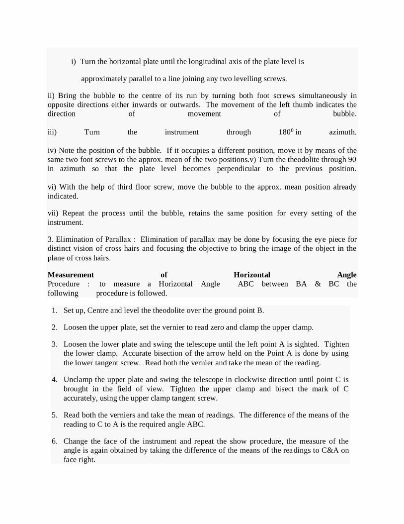
i) Turn the horizontal plate until the longitudinal axis of the plate level is

approximately parallel to a line joining any two levelling screws.

ii) Bring the bubble to the centre of its run by turning both foot screws simultaneously in

opposite directions either inwards or outwards. The movement of the left thumb indicates the

direction of movement of bubble.

iii) Turn the instrument through 1800 in azimuth.

iv) Note the position of the bubble. If it occupies a different position, move it by means of the

same two foot screws to the approx. mean of the two positions.v) Turn the theodolite through 90

in azimuth so that the plate level becomes perpendicular to the previous position.

vi) With the help of third floor screw, move the bubble to the approx. mean position already

indicated.

vii) Repeat the process until the bubble, retains the same position for every setting of the

instrument.

3. Elimination of Parallax : Elimination of parallax may be done by focusing the eye piece for

distinct vision of cross hairs and focusing the objective to bring the image of the object in the

plane of cross hairs.

Measurement of Horizontal Angle

Procedure : to measure a Horizontal Angle ABC between BA & BC the

following procedure is followed.

1. Set up, Centre and level the theodolite over the ground point B.

2. Loosen the upper plate, set the vernier to read zero and clamp the upper clamp.

3. Loosen the lower plate and swing the telescope until the left point A is sighted. Tighten

the lower clamp. Accurate bisection of the arrow held on the Point A is done by using

the lower tangent screw. Read both the vernier and take the mean of the reading.

4. Unclamp the upper plate and swing the telescope in clockwise direction until point C is

brought in the field of view. Tighten the upper clamp and bisect the mark of C

accurately, using the upper clamp tangent screw.

5. Read both the verniers and take the mean of readings. The difference of the means of the

reading to C to A is the required angle ABC.

6. Change the face of the instrument and repeat the show procedure, the measure of the

angle is again obtained by taking the difference of the means of the readings to C&A on

face right.

7. The mean of the two measures of the angle ABC on two faces is the required value of the

angle ABC.

Fig 9.1 Parts of theodolite

Fig 9.2 Measurement with thodolite

Fig 9.3 Reading a theodolite

Fig 9.4 Measurement of Angle ABC

Measurement of Angle ABC

—The instrument is set over B.

—The lower clamp is kept fixed and upper clamp is loosened.

—Turn the telescope clockwise set vernier A to 0° and vernier B to approximately 180°.

—Upper clamp is tightened and using the upper tangent screw the vernier A and B are

exactly set to 0° and 180°.

—Upper clamp is tightly fixed, lower one is loosened and telescope is directed towards A

and bisect the ranging rod at A.

—Tightened the lower clamp and turn the lower tangent screw to perfectly bisect ranging

rod at A.

—Loose the upper clamp and turn the telescope clockwise to bisect the ranging rod at C

tightened the upper clamp and do the fine adjustment with upper tangent screw.

—The reading on vernier A and B are noted. Vernier A gives the angle directly and

vernier B gives the reading by subtracting the initial reading (180°) from final reading

Vertical angle measurement-1

1. The theodolite is set up at O. It is centred and levelled properly. The zeros of the vernires

(generally C and D) are set at the 0° - 0° mark of the vertical circle (which is fixed to the

telescope). The telescope is then clamped.

2. The plate bubble is brought to the centre with the help of food screws (in the usual

manner). Then the altitude bubble is brought to the centre by means of a clip screw. At

this position the line of collimation is exactly horizontal.

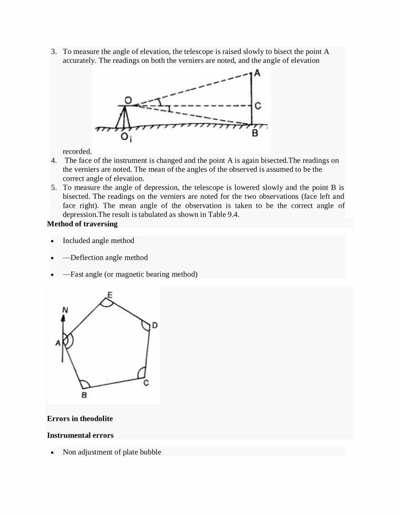
3. To measure the angle of elevation, the telescope is raised slowly to bisect the point A

accurately. The readings on both the verniers are noted, and the angle of elevation

recorded.

4. The face of the instrument is changed and the point A is again bisected.The readings on

the verniers are noted. The mean of the angles of the observed is assumed to be the

correct angle of elevation.

5. To measure the angle of depression, the telescope is lowered slowly and the point B is

bisected. The readings on the verniers are noted for the two observations (face left and

face right). The mean angle of the observation is taken to be the correct angle of

depression.The result is tabulated as shown in Table 9.4.

Method of traversing

Included angle method

—Deflection angle method

—Fast angle (or magnetic bearing method)

Errors in theodolite

Instrumental errors

Non adjustment of plate bubble

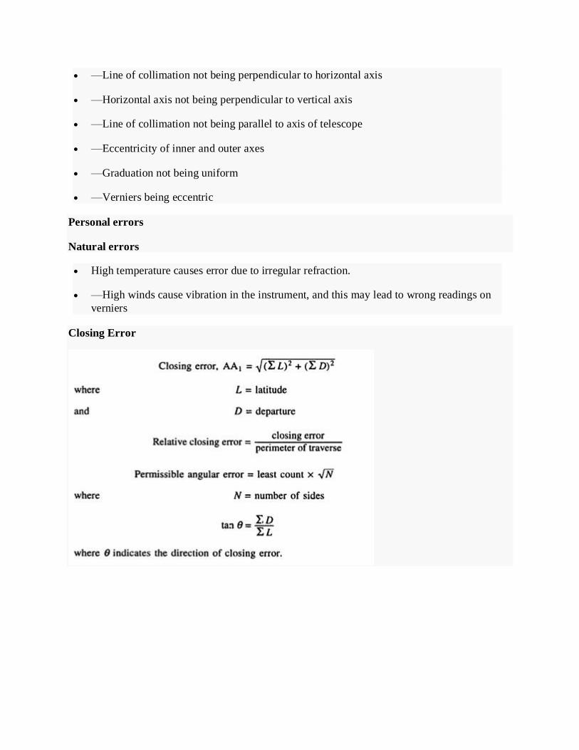
—Line of collimation not being perpendicular to horizontal axis

—Horizontal axis not being perpendicular to vertical axis

—Line of collimation not being parallel to axis of telescope

—Eccentricity of inner and outer axes

—Graduation not being uniform

—Verniers being eccentric

Personal errors

Natural errors

High temperature causes error due to irregular refraction.

—High winds cause vibration in the instrument, and this may lead to wrong readings on

verniers

Closing Error

Lesson 16. Introduction to setting of curves

Curves are regular bends provided in the lines of communication like roads, railways and canals

etc. to bring about gradual change of direction.

They enable the vehicle to pass from one path on to another when the two paths meet at an angle.

They are also used in the vertical plane at all changes of grade to avoid the abrupt change of

grade at the apex.

HORIZONTAL CURVES

Curves provided in the horizontal plane to have the gradual change in direction are known as

horizontal curves.

VERTICAL CURVES

Curves provided in the vertical plane to obtain the gradual change in grade are called as vertical

curves.

Curves may be circular or parabolic. Curves are generally arcs of parabolas.

Curves are laid out on the ground along the centre line of the work.

NEED FOR PROVIDING CURVES

Curves are needed on Highways, railways and canals for bringing about gradual change of

direction of motion. They are provided for following reasons:-

i) To bring about gradual change in direction of motion.

ii) To bring about gradual change in grade and for good visibility.

iii) To alert the driver so that he may not fall asleep.

iv) To layout Canal alignment.

v) To control erosion of canal banks by the thrust of flowing water in a canal.

CLASSIFICATION OF CURVES

Most types of transportation routes, such as highways, railroads, and pipelines, are connected by

curves in both horizontal and vertical planes.

Horizontal Curves: Curves used in horizontal planes to connect two straight tangent sections.

Two types of horizontal cures:

Circular arcs, and

Spirals

Simple Curve: A circular arc connecting two tangents.

Compound Curve: Two or more circular arcs of different radii tangent to each other.

Broken-back Curve: Combination of a short length of tangent connecting two circular arcs that

have centers on the same side.

Reverse Curve: Two circular arcs tangent to each other, with their centers on opposite side of

the alignment.

Circular curves are further classified as :

1. Simple Curves.

2. Compound Curves.

3. Serpentine Curves.

4. Deviation Curves.

1. Simple Curve:

A simple curve Consists of a single arc of circle connecting two straights. It has radius of the

same magnitude throughout.

2. Compound Curves.

A compound Curve consists of two or more simple curves having different radii bending in the

same direction and lying on the same side of the common tangent. Their centres lie on the same

side of the curve.

3. Reverse or serpentine curve

A reverse or serpentine curve is made up of two arcs having equal or different radii bending in

opposite direction with a common tangent at their junction . Their centres lie on opposite sides of

the curve. Reverse curves are used when the straights are parallel or intersect at a very small

angle.

4. Deviation curve

A deviation curve is simply a combination of two reverse curves. it is used when it becomes

necessary to deviate from a given straight path in order to avoid intervening obstructions such as

bend of river, a building , etc.

They should be avoided as far as possible on main lines and highways where speeds are

necessarily high.

Degree of Circular Curve

The rate of curvature of circular curves can be designated either by their radius (100-m

curve), or by their degree of curve.

The degree of curve:

Arc definition: The central angle subtended by a circular arc of 30m (100-ft).

Chord definition: The angle at the center of a circular arc subtended by a chord of 30m

(100 ft).

Definitions and Derivation of Circular Curve Formulas (Ref Fig.)

PI: Point of intersection

PC: Point of curvature (the beginning of the curve)

PT: Point of tangency (the end of the curve)

TC: Tangent to curve

CT: Curve to tangent

R: Curve radius

T: Tangent distance (PC-PI or PI-PT)

LC: Long chord (PC-PT)

L: Length of the curve (along the curve)

E: Length from the PI to the curve midpoint on a radial line.

M: Middle ordinate. The radial distance from the midpoint of the long chord to the curves

midpoint.

POC: Any point on curve.

POT: Any point on tangent.

Da: Degree of any curve (arc definition)

Dc: Degree of any curve (chord definition)

I: Intersection angle (central angle)

FIG. CIRCULAR CURVE ELEMENTS

Stationing

Stationing: In route surveying, stationing is used to specify the relative horizontal positioning of

any point along the reference line. The starting point is usually designated with some arbitrary

value.

English Unit System:

Starting point: Usually 10 + 00 ft or 100 + 00 ft is selected.

Metric Unit System:

Starting point: Usually 1 + 000 km or 10 + 00 km is selected. In rural areas, the spacing is

usually taken as 10, 20, 30, and 40m.

Circular Curve Stationing

The beginning point of any project is assign a station value, and all other points along the

reference line are then related to it.

After the tangents have been staked and stationed, the I angle is observed at each PI, and curves

computed and staked.

General Procedure of Circular Curve Layout by Deflection Angles

Layout of a curve by deflection angles can be done by

The incremental chord method, and

The total chord method

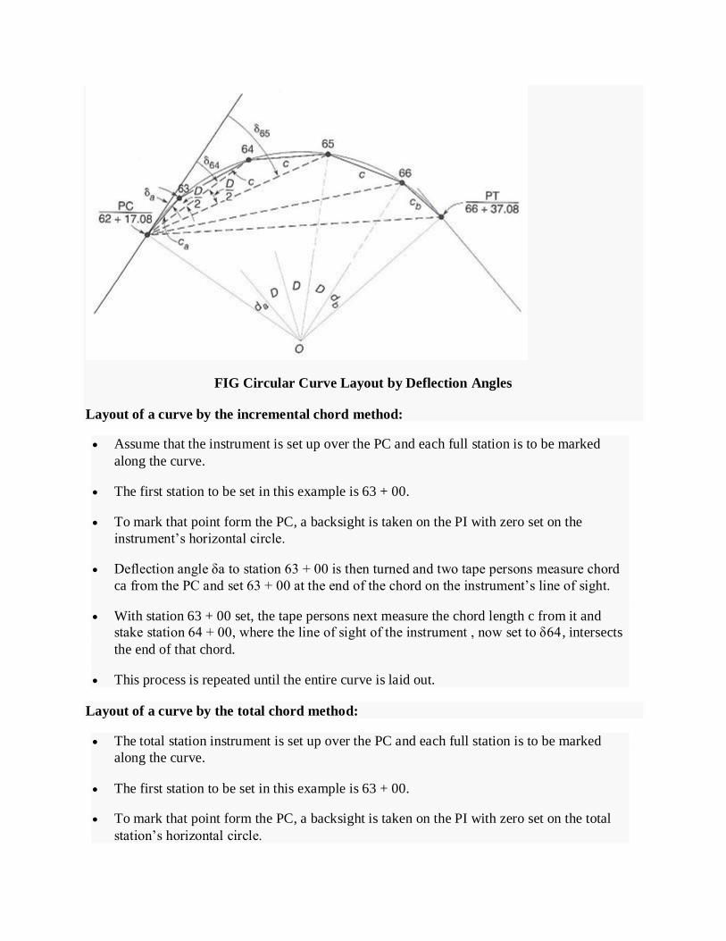
FIG Circular Curve Layout by Deflection Angles

Layout of a curve by the incremental chord method:

Assume that the instrument is set up over the PC and each full station is to be marked

along the curve.

The first station to be set in this example is 63 + 00.

To mark that point form the PC, a backsight is taken on the PI with zero set on the

instrument’s horizontal circle.

Deflection angle δa to station 63 + 00 is then turned and two tape persons measure chord

ca from the PC and set 63 + 00 at the end of the chord on the instrument’s line of sight.

With station 63 + 00 set, the tape persons next measure the chord length c from it and

stake station 64 + 00, where the line of sight of the instrument , now set to δ64 , intersects

the end of that chord.

This process is repeated until the entire curve is laid out.

Layout of a curve by the total chord method:

The total station instrument is set up over the PC and each full station is to be marked

along the curve.

The first station to be set in this example is 63 + 00.

To mark that point form the PC, a backsight is taken on the PI with zero set on the total

station’s horizontal circle.

Deflection angle δa to station 63 + 00 is then turned and the reflector placed on line and

adjusted until its distance from the instrument is ca from the PC and the stake set at 63 +

00.

To set station 64 + 00, the deflection angle δ64 is turned, reflector placed on this line of

sight, and adjusted in position until the total chord from the PC to station 64 + 00 is

obtained, and the stake set.

This process is repeated until the entire curve is laid out.

Computing Deflection Angles and Chords

For deflection angle method, deflection angles and chords are important values that must

be calculated.

To stake the first station,which is normally an odd

distance from the PC (shorter than a full-station increment), subdeflection angle δa and subchord

ca are needed.

Central angle da subtended by arc sa from the PC to 63 + 00 is calculated by proportion

da/sa = I/L from which da= sa I / L

Theorem: The angle at a point between a tangent and any chord is equal to half the central angle

subtended by the chord.

Thus subdeflection angle δa needed to stake station 63 + 00 is da/2, or da= sa I / 2L.