Lectures on Three-Dimensional Elasticitypubl/ln/tifr71.pdf · Lectures on Three-Dimensional...
135
Lectures on Three-Dimensional Elasticity By P. G. Ciarlet Tata Institute of Fundamental Research Bombay 1983
Transcript of Lectures on Three-Dimensional Elasticitypubl/ln/tifr71.pdf · Lectures on Three-Dimensional...
Lectures onThree-Dimensional Elasticity
By
P. G. Ciarlet
Tata Institute of Fundamental ResearchBombay
1983

Lectures onThree-Dimensional Elasticity
ByP. G. Ciarlet
Lectures delivered at the
Indian Institute of Science, Bangalore
under the
T.I.F.R.I.I.Sc. Programme in Applications of
Mathematics
Notes by
S. Kesavan
Published for the
Tata Institute of Fundamental Research
Springer-Verlag
Berlin Heidelberg New York
1983

©Tata Institute of Fundamental Research, 1983
ISBN 3-540-12331-8 Springer-Verlag, Berlin. Heidelberg.New YorkISBN 0-387-12331-8 Springer-Verlag, New York, Heidelberg. Berlin
No part of this book may be reproduced in anyform by print, microfilm or any other means with-out written permission from the Tata Institute ofFundamental Research, Colaba, Bombay 400 005
Printed by M. N. Joshi at The Book Centre Limited,Sion East, Bombay 400 022 and published by H. Goetze,
Springer-Verlag, Heidelberg, West Germany
Printed in India

These Lecture Notes are dedicated toProfessor K.G. Ramanathan

Avant-Propos
When studying any physical problem in Applied Mathematics,three es- 1
sential stage are involved.
1. Modelling: An appropriate mathematical model, based on thephysics or the engineering of the sitution, must be found. Usu-alluy these models are givena pariori by the physicists or theengineers themselves. However, mathematicians can also play animportant role in this process especially considering the increas-ing emphasis on non - linear models of physical problems.
2. Mathematical study of the model: A model usally involves aset ofordinary’ or partial differential equations or an (energy) functionalto be minimized. One of the first tasks is to find a suitable func-tional space in which to study the problem. Then comes the studyof existence and uniqueness or non -uniqueness of solutions. Animportant feature of linear theories is the existence of unique so-lutions depending continuoussly on the data (Hadamard’s defini-tion of well - posed problems). But with non-linear problems,non-uniqueness is a prevealent phenomenon. For instance, bifu-racation of solutions is of special interest.
3. Numerical analysis of the model: By this is meant the descrip-tion of, and the mathematical analysis of, approximation schemes,whichcanbe run on a computer in a ‘reasonable’ time to get ‘rea-sonably accurate’ answers.
In the following set of lectures the first two of the above aspects willbe studied with reference to the theory of elasticity in three dimensions.
v

vi
In the first chapter a non-linear system of partial differential equa-2
tions will be established as a mathematical model of elasticity. Thenon-linearity will appear in the highest order terms and this is an impor-tant source of difficulties. An energy functional will be established andit will be seen that the equations of equilibrium can be obtained as theEuler equations starting from the energy functional.
Existence results will be studied in the second chapter. Thetwoimportant tools will be the use of the implicit function theorem and thetheory of J. BALL.

Contents
Avant-Propos v
1 Description of Three - Dimensional Elasticity 11.1 Geometrical Preliminaries . . . . . . . . . . . . . . . . 11.2 Euilibrium Equations . . . . . . . . . . . . . . . . . . . 81.3 Constitutive Equations . . . . . . . . . . . . . . . . . . 191.4 Hyperelasticity . . . . . . . . . . . . . . . . . . . . . . 37
2 Some Mathematical Aspects of Three-Dimensional..... 532.1 General Considerations. . . . . . . . . . . . . . . . . . . 542.2 The Linearized System of Elasticity . . . . . . . . . . . 622.3 Existence Theorems via Implicit Function Theorem . . . 682.4 Convergence of Semi-Discrete... . . . . . . . . . . . . . 802.5 An Existence Theorem for Minimizing Functionals..... .842.6 J. BALL’S Polyconvexity and Existence Theorems..... . .90
Bibliography, Comments and some Open Problems 108
Bibliography 113
List of Notations 120
Index 126
vii
viii CONTENTS

Chapter 1
Description of Three -Dimensional Elasticity
THIS CHAPTER WILL be divided into four sections. In the first sec- 3
tion some preliminaries on deformations inR3 will be discussed; thesecond will be devoted to the equations of eqilibrium and thethird toconstitutive equations. These together will give rise to the boundaryvalue problem which will serve as the model for three - dimensionalelasticity. The last section will describe the energy functional and theassociated Euler equations will be seen to give the equations of equilin-rium and the constitutive equations.
1.1 Geometrical Preliminaries
Let Ω ⊂ R3 be a bounded open set. LetBR = Ω, the closure ofΩ inR
3, stand for thereference configuration. (The subsriptR will alwaysstand for the reference configuration.) LetXR be a generic point inBR.If e1, e2, e3 is the standard orthonormal basis forR3,
(1.1-1) OXR = XRi ei
whereOXR stands for the position vector ofXR. (In the above relation 4
and in all that follows, the summation convention for repeated indiceswill always be adopted.)
1
2 1. Description of Three - Dimensional Elasticity
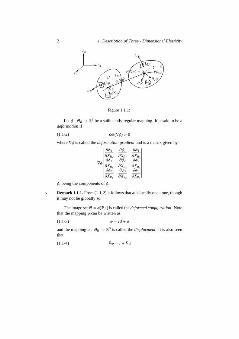
Figure 1.1.1:
Let φ : BR→ R3 be a sufficiently regular mapping. It is said to be adeformationif
(1.1-2) det(∇φ) > 0
where∇φ is called thedeformation gradientand is a matrix given by
∇φ
∣
∣
∣
∣
∣
∣
∣
∣
∣
∣
∣
∣
∣
∣
∣
∣
∂φ1
∂XR1
∂φ1
∂XR2
∂φ1
∂XR3∂φ2
∂XR1
∂φ2
∂XR2
∂φ2
∂XR3∂φ3
∂XR1
∂φ3
∂XR2
∂φ3
∂XR3
∣
∣
∣
∣
∣
∣
∣
∣
∣
∣
∣
∣
∣
∣
∣
∣
φi being the components ofφ.
Remark 1.1.1.From (1.1-2) it follows thatφ is locally one - one, though5
it may not be globally so.
The image setB = φ(BR) is called thedeformed configuration. Notethat the mappingφ can be written as
(1.1-3) φ = Id + u
and the mappingu : BR→ R3 is called thedisplacment. It is also seenthat
(1.1-4) ∇φ = I + ∇u
1.1. Geometrical Preliminaries 3
whereI is the identity matrix and∇u is thedisplacement gradient.The deformation gradient defines the deformation atX = φ(XR) up
to first order. Ifdt e1 is a line segment parallel toe1 at XR, it is trans-formed into a curve atX whose tangent isdt ∂1φ, where∂1φ is the firstcolums vector of∇φ. The magnitude dt is now ‘streched’ by dt|∂1φ|,where|.| stands for the Euclidean norm. The three vectors∂1φ, ∂2φ, ∂3φ
are independent and, owing to the relation (1.1-2), preserve the orienta-tion of e1, e2, e3.
It will now be seen how volume, area and line elements are trans-formed under the defomationφ.
(i) Volume elements:The change from a volume elementdXR to dXin the deformed confirguration comes from the familiar change ofvariable formula in interation theory:
(1.1-5) dx= det(∇φ(XR))dXR.
(ii) Surface elements:If dAR is a surface element onBR deformedonto a surface elemmentdA onB, then
(1.1-6) dA= det(∇φ(XR))|(∇φ(XR))−tnR|dAR
wherenR is the unit outer normal. (IfF is any matrix,FT stands 6
for its transpose,F−1 for its inverse andF−T = (F−1)T).
The formula (1.1-6) will now be proved . This needs some prelim-inaries. LetM3 stand for the set of all 3×3 matrices. A tensor willbe understood simply to be an element ofM3.
Let T : B→ M3 be a tensor field. Then itsdivergence(assumingTto be smooth snough) is defined by
(1.1-7) DIVT =∂Ti j
∂X jei .
Thus each component ofDIV T is the divergence (in the usualsence) of the correspondingrow vector ofT. By a standard applicationof Green’s formula it follows that
(1.1-8)∫
B
DIVTdX=
∫
B
∂Ti j
∂X jdX
ei =
∫
∂B
Ti j n jdA
ej =
∫
∂B
TndA
4 1. Description of Three - Dimensional Elasticity
wheren is the units outer normal toB. In the same veinDIVR(TR) ontensor fields onBR can be defined and the analogue of (1.1-8) can beobtained.
Let T : B → M3 be a tensor field. ItsPiola Transformis a tensorfield TR : BR→ M3 given by
(1.1-9) TR(XR) = det(∇φ(XR))T(X)(∇φ(XR))−T
wereX = φ(XR).This is a very useful transformation. The following theoremwill
establish the formula (1.1-6).
Theorem 1.1.1. (i) TR(XR)nRdAR = T(X)ndA7
(ii) det(Vφ(XR))(Vφ(XR))−TnRdAR = ndA
(iii) det(∇φ(XR))|(∇φ(XR))−TnR|dAR = dA.
Proof. It can be shown that (cf. Exercise 1.1-1).
(1.1-10) DIVRTR(XR) = det(Vφ(XR))DIVT(X)
If vR is any arbitrary volume inBR andϑ = φ(vR), then∫
∂vR
TR(XR)nRdAR =
∫
∂vR
DIVRTR(XR)dXR
=
∫
vR
det(∇φ(XR))DIVT(XR))dXR
=
∫
vR
DIVT(X)dX =∫
∂v
T(X)ndA
which, asv was arbritrary, proves (i). The assertion (ii) follows by set-ting T = I . This is a vector relation and taking the Euclidean norm onboth sides gives (iii).

1.1. Geometrical Preliminaries 5
Remark 1.1.2.The matrix det(∇φ)(∇φ)−T = (adj∇φ)−T is the matrix ofcofactors of∇φ.
(iii) Line elements: Ifφ is smooth enough,φ(XR + δXR) − φ(XR) =∇φ(XR)δXR+ o(δXR).
Thus
(1.1-11) |φ(XR+δXR)−φ(XR)|2 = δXTR∇φ(XR)T∇φ(XR)δXR+o(|δXR|2)
which gives the change in length. The matrix
(1.1-12) C = ∇φT∇φ
is called the(right) Cauchy - Green strain tensorand will play an im- 8
portant role in the theory. It is used to compute the length ofan arc. Iff (I ) is a curveℓR in BR, whereI ⊂ R is an interval, andℓ = φ(ℓR) is itsimage inB, then the length ofℓ is given by
∫
I
|(φo f)′(t)|dt =∫
I
√
ci j ( f (t)) f ′i (t) f ′j (t)dt
whereCi j are the components of the matrixC defined above.
Remark 1.1.3.The matrix
(1.1-13) B = ∇φ∇φT
called the(left) Cauchy-Green strain tensorwill be introduced later andwill play an important role in the constitutive equations.
Remark 1.1.4.The change in volume depends on a scalar det∇φ. Thechange is surface elements depends on a matrix, (adj∇φ) and the changein line elements on a matrix,C = ∇φT∇φ. All these will figure in theintegral representing the energy (cf. Sect. 2.6).
To conclude this section, it will now be examined to what extent thestrain tensorC is a measure of the deformation. The word ‘deformation’can be interpreted in two ways - first the formal sense as defined earlier
6 1. Description of Three - Dimensional Elasticity
in this section; secondly, in an intuitive way which can be described asfollows. If φ were merely to consist of a translation and then a rotationabout a point in space, while it is a deformation in the strictsense, yetdistances between points are not altered. So intuitively the body has notbeen ‘deformed’, Such a transformation is called a rigid deformation.
Thus,φ is said to be arigid deformationif
(1.1-14) φ(XR) = a+ Q(OXR),
where a∈ R3 andQ is an orthogonal matrix whose determinant is+1.9
The vector a above represents a translation and the matrixQ a rota-tion. The following notation will used for various classes of matrices:
M3+ = F ∈ M3|det(F) > 0O
3 = F ∈ M3|FTF = FFT = I O
3+ = F ∈ O3|det(F) = +1S
3 = F ∈ M3|FT = FS
3> = F ∈ S3|Fis positive definite.
ThusQ ∈ O3+ . Observe that ifφ is rigid thenC = QTQ = I . In fact,
under suitable hypotheses, the converse is also true.
Theorem 1.1.2. Let Ω be an open connected subset ofR3. Let φ ∈C1(Ω;R3) such that for all x∈ Ω,
(1.1-15) ∇φ(x)T∇φ(x) = I
Then, there exists a vector a∈ R3 and a matrix Q∈ O3 such that,for all x ∈ Ω
(1.1-16) φ(x) = a+ Q(0x).
Proof. Cf. Exercise 1.1-2
Theorem 1.1.3.LetΩ be an open connected subset ofR3 and letφ, ψ ∈C1(Ω;R3) such that for all x∈ Ω
(1.1-17) ∇φ(x)T∇ψ(x) = ∇ψ(x)T∇φ(x).
1.1. Geometrical Preliminaries 7
Assume further thatψ is one - one and thatdet(∇ψ(x)) , 0 for all10
x ∈ Ω. Then there exists a∈ R3 and Q∈ O3 such that for all x∈ Ω
(1.1-18) φ(x) = a+ Qψ(x).
Proof. Consider the mappingθ = φoψ−1 onψ(Ω). Clearlyψ(Ω) is con-nected. Also, under the given conditions, it is open by the theorem ofinvariance of domain. Further,θ ∈ C1(ψ(Ω);R3). Now from (1.1-17) itfollows thatθ satisfies (1.1-15) and so the previous theorem applies toθ
and the result follows.
Thus if two deformations have the same strain tensor then, upto arigid deformation, they are the same. ThusC ‘measures’ the ‘deforma-tion’ upto a rigid transformation. Naturally, a measure of the deviationfrom a rigid deformation is obtained fromC − I . The Green-St Venantstrain tensor, E, is defined by the relation
(1.1-19) C − I = 2E
In terms of the displacement gradient,
I + 2E = C = ∇φT∇φ = I + ∇uT + ∇u+ ∇uT∇u
or, componentwise,
(1.1-20) Ei j =12
(∂iu j + ∂ jui + ∂ium∂ jum)
where∂i stands for∂
∂XRi
Exercises
1.1-1 Prove thePiola identity 11
DIVR(det(∇φ(XR))(∇φ((XR))−T) = 0.
Deduce the relation (1.1-10) from this.

8 1. Description of Three - Dimensional Elasticity
1.1-2. Prove Theorem 1.1.2 (Hint: First show that at least locally,φ isan isometry; then show∇φ is locally contant and use the con-nectendness ofΩ.)
1.1-3. Let φ : Rn→ Rn, n ≥ 2, be continuous. Assume that there existsℓ > 0 such that for allx, y ∈ Rn with |x− y| = ℓ, |φ(x) − φ(y)| = ℓ.Show thatφ is an isometry, i.e. there existsa ∈ Rn andQ ∈ On
such that for allx ∈ Rn
φ(x) = a+ Qx.
1.1-4. Given a tensor fieldΓ : Ω → S3, find necessary and sufficientconditions such that there exists a mappingφ : Ω→ Rn with
Γ = ∇φT∇φ
1.2 Euilibrium Equations
The equilibrium equations give the relationship between the given forcesacting on a body and the state of “stress” (to be defined below)whichresults as a consequence of these forces.
Let the mass density asX ∈ B be given byρ(X) while that atXR ∈BR is given byρR(XR). The applied forces inB are of two kinds.
Figure 1.2.1:12

1.2. Euilibrium Equations 9
(i) Body (or volumic) forces: b: B → R3. The elementary force ona volume elementdX will thus beρ(X)b(X)dX. An example of abody force is gravity and in this caseb = (o, o,−g).
(ii) Applied surface forces: t1 : ∂B1 → R3, where∂B1 is a portion ofthe boundary∂B. If dA is a surface element, the applied force onit will be t1dA. An example of a surface force is a pressure loadwheret1 = −pn, p ∈ R, n the normal todA.
A system of forcesin B consists ofbody forces(identical to (i)above) andsurface forces t: B × Σ1 → R3 whereΣ1 is the unit spherein R3, i.e.,
Σ1 = x ∈ R3||x| = 1.If ϑ is any subvolume ofB, dA a surface element of∂ϑ andn the
normal to it, the surface forcet(X, n)dA acts in it. Note that this is inde-pendent ofϑ, i.e. if ϑ1 were another subvolume anddA lay on∂v1 withthe samen as normal, the force acting on it will remain ast(X, n)dA. 13
Further ifdA⊂ ∂B andn were also normal to∂B, it is required that
(1.2-1) t(X, n) = t1(X).
The vectort(X, n) is called theCauchy stress vector.The following axiom is the basis of Continuum Mechanics in gen-
eral, and consequently of the theory of elasticity in particular.
AXIOM OF STATIC EQUILIBRIUM. LetB be a deformed configu-ration in static equilibrium. There exists a system of forces such that forany subdomainϑ ⊂ B,the corresponding system of forces is equivalentto zero (in the sense of torsors). Thus
∫
ϑ
ρ(X) b(X) dX +∫
∂ϑ
t(X, n) dA= o.(1.2-2)
∫
ϑ
OXΛρ(X)b(X)dX+∫
∂ϑ
OXΛt(x, n)dA= o.(1.2-3)
The wedgeΛ stands for the usual cross product of vectors inR3.The following notation will be useful in manipulating crossproducts.

10 1. Description of Three - Dimensional Elasticity
For indicesi, j, k taking values 1, 2, 3 the tensor of rank 3, ǫi jk , isdefined by
(1.2-4) ǫi jk =
+1 if(i, j, k)is an even permutation of(1, 2, 3),
−1 if it is an odd permutation of(1, 2, 3),
0 otherwise.
Then for vectora, bǫR3,
(1.2-5) aΛb = ǫi jka jbkei .
The following consequence of the axiom of static equilibrium is of14
paramount importance.
Theorem 1.2.1(Cauchy’s Theorem). Let ρǫC(B ; R), bǫC(B;R3),t(., n) ǫC1(B;R3) and t(X, .)ǫC(
∑
1;R3). Then there exists a tensor fieldTǫC1 (B; M3) such that
t(X, n) = T(X)n, for all XǫB, nǫΣ1,(1.2-6)
DIVT(X) + ρ(X) b(X) = 0, for all XǫB,(1.2-7)
T(X) = TT(X), for all XǫB.(1.2-8)
Proof. Let X0 be any point inB. Consider a tetrahedronϑ with verticesX0,V1,V2,V3 as shown in Fig. 1.2.2.
Figure 1.2.2:
Let n0ǫ∑
1 be the normal to the planeV1V2V3 and keepn fixed tobegin with. Let the distance ofX to the plane beδ, let Si(i = 1, 2, 3) be

1.2. Euilibrium Equations 11
the surface opposite the vertexVi(i = 1, 2, 3) andS the surface oppositeX0. Sinceρ, b are continuous onB, they are bounded. Thus by (1.2.2),
|∫
∂ϑ
t(x, n)dA| ≤ KVol(ϑ)
K being a constant independent ofδ. Since Vol(ϑ) = K1δ3, A(δ) = Area 15
of S = K2δ2,K1,K2 being independent ofδ, it follows that
(1.2-9) limδ→O
1A(δ)
∫
∂ϑ
t(X, n)dA= 0
Now,
limδ→O
1A(δ)
∫
S
t(X, n) dA= t(XO, nO)
and
lim δ→ 01
A(δ)
∫
Si
t(X, n)dA= (nO.ei)t(XO,−ei)
using the continuity of the given functions. Hence by (1.2-9),
(1.2-10) t(X, n) = −(n.ei)t(X,−e).
If n → ej , again by continuity oft it follows that
t(X, ej) = −t(X,−ej).
Thus, on substituting this in (1.2-10),
(1.2-11) t(XO, nO) = t(XO, ej)n j .
Settingt(X, ej) = Ti j (X)ei
the equation (1.2-6) follows. The smoothness ofT results from that oftw.r.t. X.
12 1. Description of Three - Dimensional Elasticity
Using (1.2-6) in (1.2-2), for any volumeϑ,
0 =∫
ϑ
ρ(X)b(X)dX+∫
∂ϑ
T(X)ndA
=
∫
ϑ
ρ(X)b(X) + DIV(T)dX,
from which (1.2-7) follows asϑ was aribitrary.16
Finally by (1.2-3) and (1.2-5)
0 =∫
L
ǫi jk X jρ(X)bk(X)dX+∫
∂ϑ
ǫi jk X jTkℓnℓdA
= −∫
ϑ
ǫi jk X j∂Tkℓ
∂XℓdX+
∫
∂ϑ
ǫi jk X jTkℓnℓdA
=
∫
ϑ
ǫi jk∂X j
∂XℓTkℓdX =
∫
ϑ
ǫiℓkTkℓ,
using (1.2-7). Sinceϑ was arbitrary,
ǫiℓkTkℓ = 0
which is just a restatement of (1.2-8).
Remark 1.2.1.Given a tensor fieldT : B → M3 satisfying (1.2-7) and(1.2-8), the vector fieldt(X, n) = T(X)n satisfies (1.2-2) and (1.2-3).
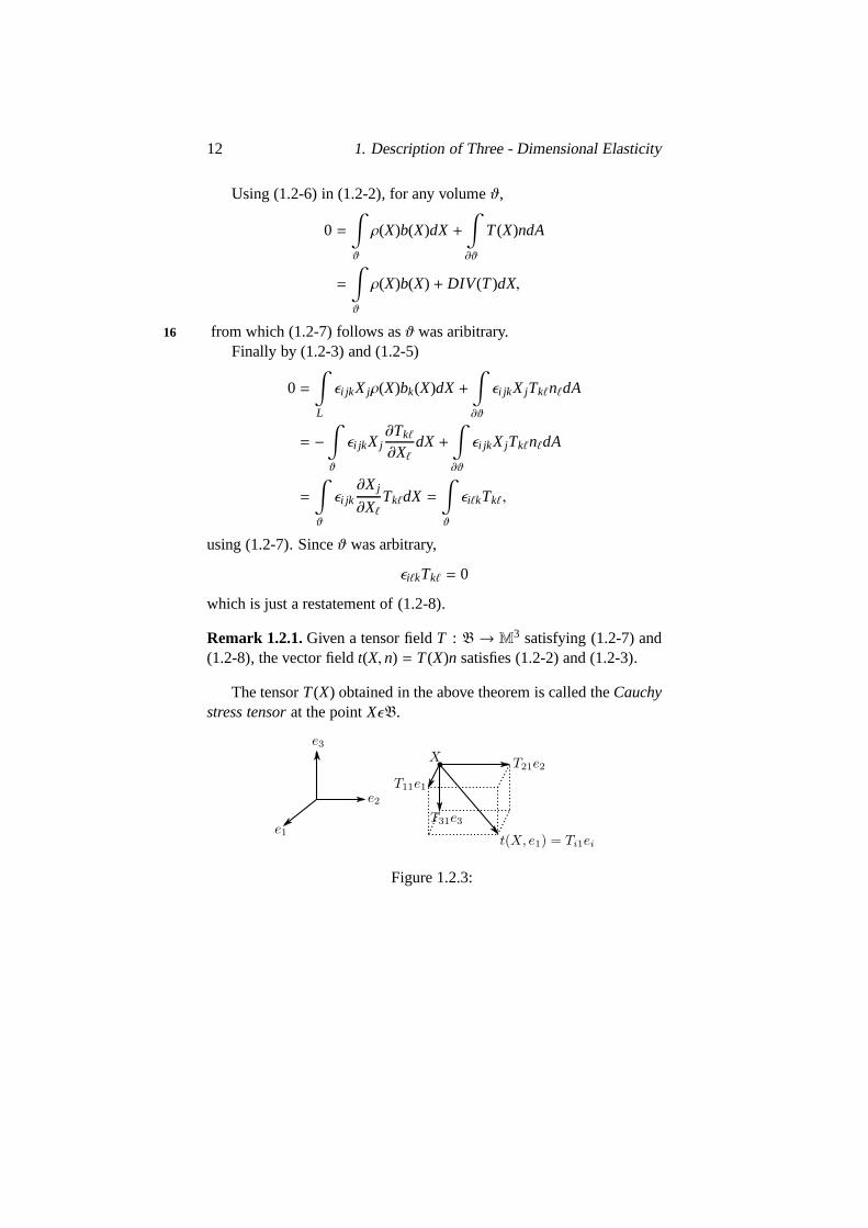
The tensorT(X) obtained in the above theorem is called theCauchystress tensorat the pointXǫB.
Figure 1.2.3:

1.2. Euilibrium Equations 13
Remark 1.2.2.The components ofT can be interpreted as follows. If 17
an elementdA has normale1 then the Cauchy stress vector acting on it,t(X, e1) has componentsT11,T21 andT31 and so on.
The Cauchy stress tensor thus satisfies a boundary value problem:
DIVT + ρb = 0
T = TT
in B
Tn = t1 on∂B1
Let u.v stand for the usual scalar product inR3, i.e. v.v = uivi . IfA, BǫM3, denote
(1.2-12) A : B = Ai j Bi j = tr(ABT).
This is an inner product inM3 with the associated norm
(1.2-13) ‖A‖ =√
Ai j Ai j .
Using Green’s formula, a variational form of the boundary valueproblem can be obtained.
If T is a tensor field andHO is a vector field onB then∫
B
DIV T.HOdX =∫
B
∂Ti j
∂X jHOidX
= −∫
B
Ti j∂HOi
∂X jdX+
∫
∂B
Ti j HOin jdA
= −∫
B
T : GRADHOdX+∫
∂B
Tn.HOdA.
In particular, ifT is a solution of the above boundary value problem18
and if HO vanishes on∂B0 = ∂B\∂B1, then Green’s formula above gives
0 =∫
B
(DIVT + ρb).HOdX

14 1. Description of Three - Dimensional Elasticity
=
∫
B
(−T : GRADHO + ρb.HO)dX+∫
∂B1
t1.HOdA.
Conversely if the above relation is satisfied for allHO vanishing on∂B0 thenT is a solution of the boundary value problem. Thus
Theorem 1.2.2.The following are equivalent:
(i)
DIVT + ρb = 0, inB
Tn = t1 in ∂B1
(ii) For all HO : B→ R3, HO vanishing on∂BO,
(1.2-14)∫
B
T : GRADHOdX =∫
ρb.HOdX+∫
∂B1
t1.HOdA.
The equations (1.2-14) form the so-calledvariantional formulationof the boundary value problelm (i). In Mechanics, it is also known asthePrinciple of Virtual Work in the deformed configuration.
The equations of equilibrium were established in theEulerian vari-able, X, in the deformed configuration. However, this is of no use forcomputation as the deformationφ is unknown. So, the equations mustbe written in the reference configuration, which is afixed domaingivena priori, in terms of theLagrangian variable, XR. In doing this, it isdesirable to retain as much of thedivergence formof the equations aspossible so that a similar variational formulation can be obtained in thereference configuration. It is here that the merit of the Piola transformis seem.
The Piola transform of the Cauchy stress tensorT, called thefirst19
Piola-Kirchhoff stress tensor, is denoted byTR. Thus surya
TR = det(∇φ)T(∇φ)−T .
1.2. Euilibrium Equations 15
Figure 1.2.4:
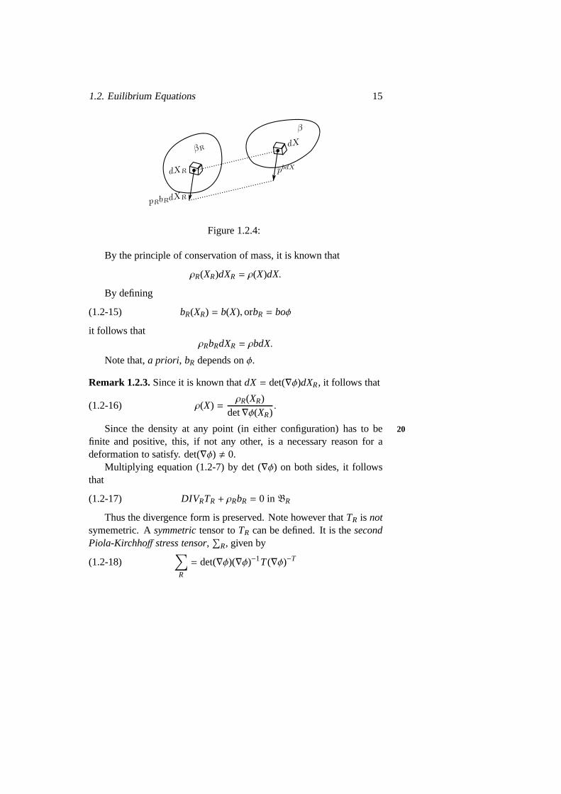
By the principle of conservation of mass, it is known that
ρR(XR)dXR = ρ(X)dX.
By defining
(1.2-15) bR(XR) = b(X), orbR = boφ
it follows thatρRbRdXR = ρbdX.
Note that,a priori, bR depends onφ.
Remark 1.2.3.Since it is known thatdX = det(∇φ)dXR, it follows that
(1.2-16) ρ(X) =ρR(XR)
det∇φ(XR).
Since the density at any point (in either configuration) has to be 20
finite and positive, this, if not any other, is a necessary reason for adeformation to satisfy. det(∇φ) , 0.
Multiplying equation (1.2-7) by det (∇φ) on both sides, it followsthat
(1.2-17) DIVRTR + ρRbR = 0 inBR
Thus the divergence form is preserved. Note however thatTR is notsymemetric. Asymmetrictensor toTR can be defined. It is thesecondPiola-Kirchhoff stress tensor,
∑
R, given by
(1.2-18)∑
R
= det(∇φ)(∇φ)−1T(∇φ)−T

16 1. Description of Three - Dimensional Elasticity
It is related toTR by
(1.2-19)∑
R
= (∇φ)−1TR.
Remark 1.2.4.It is understandable thatTR is not symmetric as it be-longs partly to the reference configuration and partly to thedeformedconfiguration and symmetry does not make much sense in such a situa-tion.
Now we turn to the transformation of the surface forces. ThefirstPiola-Kirchhoff stress vectoris defined so that
(1.2-20) tR(XR, nR) = TR(XR)nR.
Figure 1.2.5:
Recall thatTR(XR)nRdAR = T(X)ndAand so21
tR(XR, nR)dAR = t(X, n)dA.
If ∂B1R is the portion of∂BR mapped byφ onto ∂B1, definet1R :∂B1R → R3 by t1RdAR = t1dA. Again, a priori, t1R depends onφ.Explicitly, by Theorem 1.1.1,
(1.2-21) t1R(XR) = det(∇φ(XR))|(∇φ(XR))−TnR|t1(φ(XR)).
The following result is easy to establish.
Theorem 1.2.3.The equilibrium equations in the reference configura-tion are given by
DIVRTR+ ρRbR = o inBR(1.2-22)
1.2. Euilibrium Equations 17
(∇φ)TTR = TR(∇φ)T inBR(1.2-23)
TRnR = tRon∂BR.(1.2-24)
Equivalently, in terms of∑
R
DIVR(∇φ∑
R
) + ρRbR = 0 in BR(1.2-25)
∑
R
=
T∑
R
in BR(1.2-26)
∇φ∑
R
nR = t1R on∂B1R.(1.2-27)
Again, this is equivalent to the variational equations
(1.2-28)∫
BR
TR : ∇θdXR =
∫
BR
ρRbR.θdXR+
∫
∂B1R
t1R.θdAR
for all θ : BR→ R3 vanishing on∂BoR = ∂BR\∂B1R.
Remark 1.2.5.Equations (1.2-28) go under the name of the principle of22
virtual work in the reference configuration.
To conclude this section, some classes of applied forces areconsid-ered. Recall that whileρR is completely known,bR and t1R depend ingeneral onφ which is unknown.
A body force (resp. applied surfaces force) is adead loadif bR (resp.t1R) is a function ofXR only, independent ofφ.
An example of a body force which is a dead load is gravity whichis constant;b = (o, o,−g). A trivial example of an applied surface forcewhich is a dead load ist1 = 0! The pressure is an example of an appliedsurface force which isnot a dead load:
(1.2-29) t1 = −pn
wherep > o indicates an inward directed force (pressure) andp < 0indicates one which is directed outward (traction). Now
t1R = −pdet(∇φ)(∇φ)−TnR on∂BR
18 1. Description of Three - Dimensional Elasticity
which clearly depends onφ!A body force is said to beconservativeif there exists a function
β : R3 ×BR→ β(φ,XR)ǫR, such that
(1.2-30) bR(XR) = ∇φβ(φ(XR),XR),
for all XRǫBR and all deformationsφ. If which is the case then
(1.2-31)∫
BR
ρRbR.θdXR = B(φ)(θ)
where
(1.2-32) B(ψ) =∫
BR
ρR(XR)β(ψ(XR),XR)dXR.
A body force which is a deal load is conservative, β(Φ,XR) = bR(XR).23
Φ.An applied surface force isconservativeif there exists a function
τ1 : R3 × ∂B1R→ τ1(φ,XR)ǫR such that
(1.2-33) t1R(XR) = ∇Φτ1(φ(XR),XR).
Then again
(1.2-34)∫
∂B1R
t1R.θdAR = T′1(φ)(θ)
where
(1.2-35) T1(ψ) =∫
∂B1R
τ1(ψ(XR),XR)dAR.
An applied surface force which is a deal load is conservative;τ1(φ,XR) = t1R(XR).Φ. A pressure load is conservative (Exercise 1.2-3).
Exercises

1.3. Constitutive Equations 19
1.2-1 . (Da Silva’s Theorem). Given any system of applied forces (with∂B1 = ∂B) show that there existsQǫO3 such that
∫
B
ρ(X)OXΛQb(X)dX+∫
∂B
OXΛQt(X)dA= o
∫
B
ρ(X)QT(OX)Λb(X)dX+∫
∂B
QT(OX)Λt(X)dA= o.
How many solutions exist?
1.2-2. Show that the fundamental axiom of static equilibrium is equiv-alent to
∫
ϑ
ρ(X)b(X).v(X)dX+∫
∂ϑ
t(X, n).v(X)dX = 0
for every volumeϑ ⊂ B and for everyinfinitesimal rigid dis- 24
placement v, i.e.,
v(x) = a+ bΛOx, a, bǫR3.
This is sometimes also called the principle of virtual work.1.2−3.
1.2-3 Show that a pressure load is conservative.
1.3 Constitutive Equations
Given a body acted on by a system of forces, one’s main objective isto compute the deformationφ which has 3 component functions. Asa naturalintermediary, the stress tensorT has come in which has 6components (taking into account its symmetry). But so far, the boundaryvalue problem obtained via the equilibrium equations has yielded only3 equations (cf. (1.2-7)). Thus 6 more equations must be found.
From the physical point of view, observe that in obtaining the equi-librium equations, no property of the material under consideration has

20 1. Description of Three - Dimensional Elasticity
been used. Since different materials react differently to the same forces,obviously these equations alone cannot describe the response of the ma-terial.
Thus one is led to finding more equations to complete the system. Amaterial is said to beelasticif there exists a mapping
T : FǫM3+ → T(F)ǫS3
such that for any deformed configuration and any pointX = φ(XR),25
(1.3-1) T(X) = T(∇Φ(XR)).
The mapT is called theresponse functionand (1.3-1) is called aconstitutive equation.
Remark 1.3.1.The mapT above does not depends explicitly onXR.Such that a material is calledhomogeneous.If it were that
T(X) = T(XR,∇Φ(XR))
the material would be called anon-homogeneouselastic material.
If TR is the Piola transform ofT then it follows that
(1.3-2) TR = det(∇φ)T(∇φ)(∇φ)−1 def= TR(∇φ)
which gives a reponse fucntionTR : M3+ → M3 for TR. Similarly it is
possible to write one forΣR in terms of a response functionΣR : M3+ →
S3.
Theorem 1.3.1(Polar Factorisation). Let F be an invertible matrix.Then there exist an orthogonal matrix R and symmetric, positive defi-nite matrices U and V such that
(1.3-3) F = RU = VR.
Such a factorization is unique.
Proof. Cf. Exircise 1.3-1.

1.3. Constitutive Equations 21
Remark 1.3.1′. If F ∈ M3+ thenR ∈,O3
+. If G ∈ S3> there exists a unique
matrix H ∈ S3> such thatH2 = G. It is usual to writeH = G1/2. It can be
seen thatU = (FTF)1/2 andV = (FFT )1/2, in the above theorem. Since26
V = RURT,U andV are similar. Then so areB = FFT andC = FTF.
The constitutive equation (1.3-1) can be written componentwise as
Tll (X) = Tll
(
∂φ1
∂XR1
(XR), . . . ,∂φ3
∂XR3
(XR)
)
and so on. So knowingT is the same as knowing the functionsTi j . How-ever, the functionsTi j cannot be chosen arbitrarily. They must somehowreflect anintrinsic property of the material in equation, irrespective ofthe coordinate system chosen. This is the idea embodying the
AXIOM OF MATERIAL FRAME INDIFFERENCE. The Cauchy stressvector t(X, n) = T(X)n should be independent of the particular basis inwhich the constitutive equation is expressed.
Theorem 1.3.2.The following are equivalent.
(i) A response functionT : M3+ → S3 satisfies the axiom of material
frame indifference.
(ii) For every Q∈ O3+ and for every F∈ M3
+,
(1.3-4) T(QF) = QT(F)QT .
(iii) For every F∈ M3+ if F = RU is its polar factorisation then
(1.3-5) T(F) = RT(U)RT
(iv) There exists a mapΣR : S3> → S3 such that
(1.3-6) ΣR(F) = ΣR(FTF)
for every F∈ M3+. 27
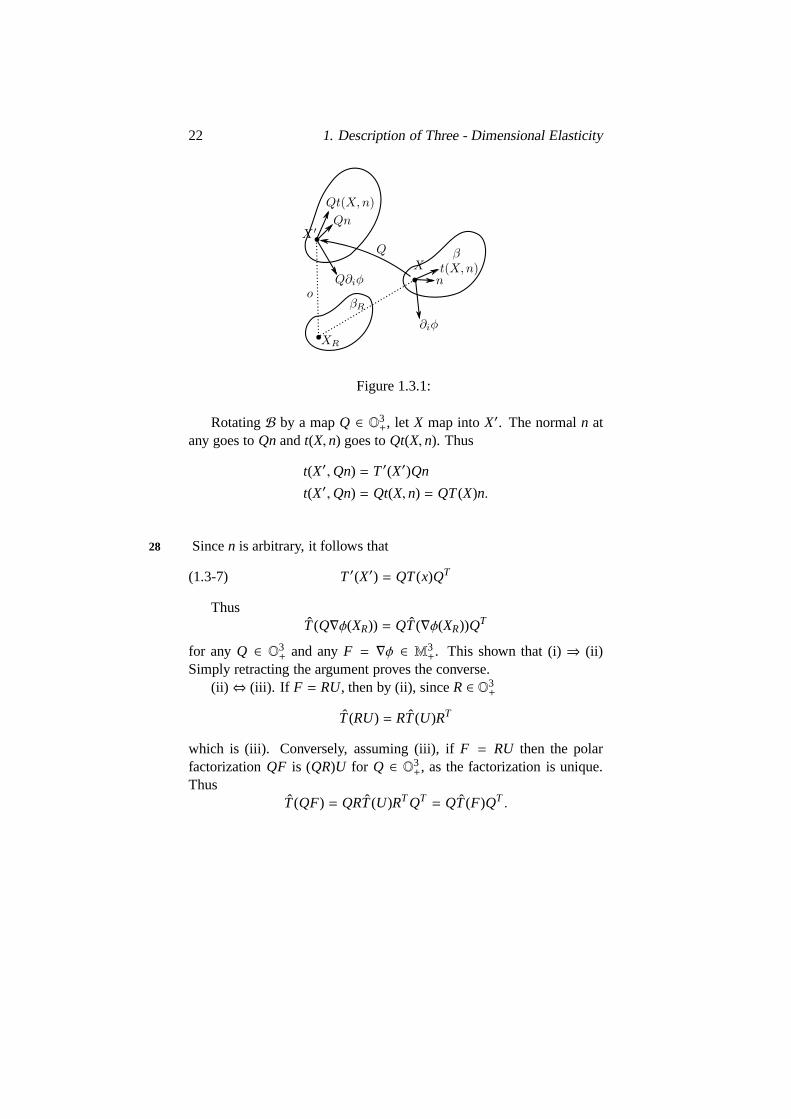
Proof. (i) ⇔ (ii) Instead of rotating the coordinate axes the same effectcan be achived by rotating the deformed configuration.
22 1. Description of Three - Dimensional Elasticity
Figure 1.3.1:
RotatingB by a mapQ ∈ O3+, let X map intoX′. The normaln at
any goes toQnandt(X, n) goes toQt(X, n). Thus
t(X′,Qn) = T′(X′)Qn
t(X′,Qn) = Qt(X, n) = QT(X)n.
Sincen is arbitrary, it follows that28
(1.3-7) T′(X′) = QT(x)QT
ThusT(Q∇φ(XR)) = QT(∇φ(XR))QT
for any Q ∈ O3+ and anyF = ∇φ ∈ M3
+. This shown that (i)⇒ (ii)Simply retracting the argument proves the converse.
(ii) ⇔ (iii). If F = RU, then by (ii), sinceR ∈ O3+
T(RU) = RT(U)RT
which is (iii). Conversely, assuming (iii), ifF = RU then the polarfactorizationQF is (QR)U for Q ∈ O3
+, as the factorization is unique.Thus
T(QF) = QRT(U)RTQT = QT(F)QT .

1.3. Constitutive Equations 23
(ii) ⇔ (vi). SinceF = RU impliesU = (FTF)1/2,
T(F) = RT(U)RT
= FU−1T(U)U−1FT
= FS(FTF)FT
whereS : S3> → S3. Conversely, ifT(F) is of the above form, then if
F = RU,T(U) = US(U2)U
and 29
T(F) = FS(FTF)FT
= FS(U2)FT
= FU−1T(U)U−1FT
= RT(U)RT .
Now
ΣR(F) = det(F)F−1T(F)F−T
= (det(FT F))1/2S(FT F) = ΣR(FTF).
Remark 1.3.2.If one of the response functions, sayΓ, can be written ofeither variablesF, FTF = C, FFT = B or E ( whereC = I + 2E), thefollowing notation will be employed when the different dependences areexpressed:
Γ = Γ(F) = Γ(FTF) = Γ(FFT) = Γ∗(E)
In the above theorem it has been proved that it is enough to knowthe action ofT on a relatively small class of matrices likeS3
>.A material or response function is said to beisotropic if the Cauchy
strees tensor (or vector) computed at a given point in the deformed con-figuration is the same if the same if the reference configuration is rotatedby any rigid defomation.

24 1. Description of Three - Dimensional Elasticity
While the axiom of material frame indifference is anaxiom to ver-ified by any response fucntion, isotropy is aproperty of a particularmaterial. There can be materials which are non-isotropic; for instance,a body up of layers of different materials.
Theorem 1.3.3.The following are equivalent.30
(i) A response functionT : M3+ → S3 is isotropic.
(ii) For every F∈ M3+ and for every Q∈ O3
+,
(1.3-8) T(F) = T(FQ).
(iii) There exists a mapT : S3> → S3 such that for every F∈ M3
+,
(1.3-9) T(F) = T(FFT ).
Proof. (i) ⇔ (ii). Let Q ∈ O3+. Rotate the reference configuration about
a pointXR so that ifXR ∈ BR then
(2) θ(XR) = XR+ QT(XRXR).
Thenφ∗ = φoθ−1.
Figure 1.3.2:
The response function is isotropic if and only if
T(X) = T(∇φ(XR)) = T(∇φ∗(XR))
1.3. Constitutive Equations 25
i.e., T(∇φ(XR)) = T(∇φ(XR)Q).
(ii) ⇔ (iii). Let FFT = GGT , F,G ∈ M3+. ThenG−1F ∈ O3
+. Hence by31
(ii)T(G) = T(G(G−1F)) = T(F).
So it is clear thatT(F) depends only onFFT . Conversely ifT(F) =T(FFT) then forQ ∈ O3
+,
T(FQ) = T(FQQTFT ) = T(FFT ) = T(F).
Remark 1.3.3.By the axiom of material frame indifference, the consti-tutive equation could be expreesed in terms of a function ofC = FTFand this involved rotating thedeformedconfigurationB. By isotropy,the same could be expressed in terms of a function ofB = FFT andthis involved rotating thereferenceconfigurationBR. Thus these twonations seem to be ‘dual’ ot each other.
Remark 1.3.4.For non-isotropic materials it can be shown that
T(F) = T(FQ)
for all F ∈ M3+ but Q variying over a subgroup ofO3
+.
In what follows, the material will allways be assumed to be isotropic.Before proving a very powerful and elgent result on the structure of
a reponse function which is isotrophic and material frame-indifferent,the following definition is needed.
Let A ∈ M3. Define ıA to be the triple (ı1(A), ı2(A), ı3(A)) whereı1(A), ı2(A) andı3(A) are the principal invariants of A, and
det(A− λI ) = −λ3 + ı1(A)λ2 − ı2(A)λ + ı3(A).(1.3-10)
If A = (ai j ) andλ1, λ2, λ3 are its eigenvalues, then
ı1(A) = aii = tr(A) = λ1 + λ2 + λ3.
(1.3-11)

26 1. Description of Three - Dimensional Elasticity
ı2(A) =12
(aii a j j − a j j ai j ) =12
((tr(A))2 − tr(A2))
= tr(adjA) = λ1λ2 + λ2λ3 + λ3λ1.(1.3-12)
ı3(A) = det(A) =16
((tr(A))3 − 3tr(A)tr(A2) + 2tr(A3)) = λ1λ2λ3.
(1.3-13)
32
Further, ifA is invertible,
(1.3-14) ı2(A) = (detA)tr(A−1).
The following theorem is one of the most important results inthetheorey of elasticity.
Theorem 1.3.4(Rivlin-Ericksen Theorem). A response functionT :M
3+ → S3 is isotropic and material frame indifferent if, and only if,
it is of theT(F) = T(FFT) where the mappingT : S3> → S3 is of the
form
(1.3-15) T(B) = βo(ıB)I + β1(ıB)B+ β2(ıB)B2
for all B ∈ S3>. whereβo, β1, β2 are real valued functions.
Proof. (i) Let T : M3+ → S3 be material frame indifferent and isotropic.
Then by isotropyT(F) = T(FFT ) for some mappingT : S3> → S3. Let
Q ∈ O3+ andB ∈ S3
>. On one hand , by isotrophy
T(QB1/2) = T(QB1/2B1/2QT) = T(QBQT).
On the other hand, by the material frame indifference,
T(QB1/2) = QT(B1/2)QT
= QT(B1/2B1/2)QT = QT(B)Q.
33
ThusT satisfies , for allQ ∈ O3+, andB ∈ S3
>
(1.3-16) T(QBQT) = QT(B)QT .

1.3. Constitutive Equations 27
Conversly, letT : S3> → S3 satisfy (1.3-16) and letT(F) = T(FTF).
Then clearly,T is isotrophic. IfQ ∈ O3+, then
T(QF) = T(QFFTQT) = QT(FFT)QT.
= QT(F)QT
and soT is material frame indefferent.Thus it is now enough to check that a mappingT : S3
> → S3 sat-isfying (1.3-16) is of the form (1.3-15). (The converse is immediate tovarify).
(ii) Let T : S3> → S3 varify (1.3-16). It will now be shown that
any matrix which diagonalizesB ∈ S3> also diagnalizesT(B), i.e., any
eigenvector ofB is an eigenvector ofT(B).Let B ∈ S3
> andQ ∈ O3+ (we can always assume that) such that
QT BQ= diag (λi)
whereλ1, λ2, λ3 are the eigenvalue ofB. Define
Q1 = diag (1,−1,−1),Q2 = diag (−1, 1,−1),Q3 = diag (−1,−1, 1).
ThenQk ∈ O3+, k = 1, 2, 3.
Also, 34
QTk QT BQQk = diagλi = QT BQ.
So,
QTk QT T(B)QQk = T(QT
k QT BQQk)
= T(QT BQ)
= QT T(B)Q.
If D = QT T(B)Q, then
QTk DQk = D, k = 1, 2, 3.
If the diagonal entries ofQk areqki (= 1 if i = k,−1 if i , k), then it
follows thatDi j = qk
i Di j qkj for all 1 ≤ i, j, k ≤ 3.
28 1. Description of Three - Dimensional Elasticity
Thus if i = k , j, then
Dk j = −Dk j or Dk j = o.
HenceD is diagonal and this proves the claim.
(iii) It will now be a shown that ifT satisfies (1.3-16) then, for allB ∈ S3
>,
(1.3-17) T(B) = bo(B)I + b1(B)B+ b2(B)B2,
bα, α = 0, 1, 2 being real valued functions onS3>.
Case 1.B has 3 distanct eigenvaluesλ1, λ2, λ3 with corresponding or-35
thonormal eigenvectorsp1, p2, p3. Then
I = p1pT1 + p1pT
2 + p3pT3(1.3-18)
B = λ1p1pT1 + λ2p2pT
2 + λ3p3pT3(1.3-19)
B2 = λ21p1pT
1 + λ22p2pT
2 + λ23p3pT
3(1.3-20)
Since theλi are distinct, the Vandermonde determinant
det
1 1 1λ1 λ2 λ3
λ21 λ2
2 λ23
is non-zero and so inS3, the span ofpi pTi , i = 1, 2, 3 is equal to that of
I , B, B2. But T(B), by step (ii) above, has the same eigenvectors asB.So
(1.3-21) T(B) = µ1p1pT1 + µ2p2pT
2 + µ3p3pT3
which implies thatT(B) ∈ spanI , B, B2.
Case 2.λ1 , λ2 = λ3. Again one can write (1.3-18) and (1.3-19). Thenthe span ofp1pT
1 andp2pT2 + p3pT
3 is that ofI andB. By step (ii), it canbe seen thatµ2 = µ3, since any non-zero vector spanned byp2 andp3 isalso an eigenvector forT(B). Thus in (1.3-21)
T(B) = µ1p1pT1 + µ2(p2pT
2 + p3pT3 )
which showsT(B) ∈ span (I , B).
1.3. Constitutive Equations 29
Case 3.λ1 = λ2 = λ3. In this case, one can similarly see thatB, T(B)36
are both scalar multiples ofI .
(iv) Case. 1.λ1, λ2, λ3 are distinct eigenvalues ofB ∈ S3>, .
Let Q ∈ O3+.
T(QBQT) = bo(QBQT)I + b1(QBQT)QBQT + b2(QBQT)QB2QT
= Q(bo(QBQT)I + b1(QBQT)B+ b2(QBQT)B2)QT
But
T(QBQT) = QT(B)QT = Q(bo(B)I + b1(B)B+ b2(B)B2)QT .
Thusbα : S3> → R, α = 0, 1, 2 satisfy the functional identity
(1.3-22) bα(QBQT) = bα(B)
for all B ∈ S3> and for allQ ∈ O3
+. Thus if Q diagnalizesB, it is seenthat such a functionbα must be a function of the eigenvalues ofB only.Now choosingQi ∈ O3
+, i = 1, 2, 3 as
Q1 =
0 1 01 0 00 0 −1
,Q2 =
−1 0 00 0 10 1 0
,Q3 =
0 0 10 −1 01 0 0
it is seen from (1.3-22) thatbα is a symmetric function ofλ1, λ2, λ3. i.e,.bα(B) = βα(tB).
This proves the theorem completely.
Theorem 1.3.5. (a) GivenBR and an isotropic material frame indif-ferent material, then in any deformed configurationB = φ(BR), theCauchy stress tensor is given by
(1.3-23) T(X) = T(∇φ(XR)) = T(∇φ(XR)∇φ(XR)T),
37
T : S3> → S3 satisfying(1.3-15).
(b) The second Piola-Kirchhoff stress tensor is given by
(1.3-24) ΣR(XR) = ΣR(∇φ(XR)) = ΣR(∇φ(XR)T∇φ(XR))

30 1. Description of Three - Dimensional Elasticity
whereΣR : S3> → S3 satisfies, for all C∈ S3
>,
(1.3-25) ΣR(C) = γo(ıc)I + γ1(ıc)C + γ2(ıc)C2.
Proof. Observe that
ΣR(F) = det(F)F−1T(F)F−T
= (det(FTF))1/2F−1T(FFT)F−T
= (detC)1/2F−1[βO(ıB)I + β1(wrB)B+ B2(ıB)B2]F−T
whereC = FTF, B = FFT . But these are similar. SoıB = ıc.Further
F−1F−T = C−1
F−1BF−T = I
F−1B2F−T = C.
By the Cayley-Hamilton theorem,
−C3 + ı1(C)C2 − ı2(C)C + ı3(C)I = 0
or C−1 =1
ı3(C)(C2 − ı1(C)C + ı2(C)I )
whereı3(C) = detC , 0. Thus it is clear from these considerations that38
ΣR can be expressed in terms ofC as in (1.3-24) - (1.3-25).
It was seen in Section 1.1 that the Green-St Venant strain tensorE, given byC = I + 2E, ‘measures’ the actual deformation. IfΣR
is sufficiently smooth it is possible to express it in terms ofE. Moreprecisely, the following result is true.
Theorem 1.3.6.LetBR be the reference configuration of an isotropic,material frame indifferent elastic material. Assume that the functionsγα, a = 0, 1, 2 of (1.3-25)are differentiable atıI = (3, 3, 1). Then
(1.3-26) ΣR = ΣR(I + 2E) = −pI + (λ(trE)I + 2µE) +O(E),
where p, λ andµ are constants.

1.3. Constitutive Equations 31
Proof. Using the relations
tr(C) = 3+ 2 tr(E)
tr(C2) = 3+ 4 tr(E) + o(E)
tr(C3) = 3+ 6 tr(E) + o(E)
and the relations (1.3-11) - (1.3-13), it follows that
ı1(C) = 3+ 2 tr(E)
ı2(C) = 3+ 4 tr(E) + o(E)
ı3(C) = 1+ 2 tr(E) + o(E)
so that
γ(ıC) = γ(ıI ) + (2∂γ
∂ıI(ıI ) + 4
∂γ
∂ı2(ıI ) + 2
∂γ
∂ı3(ıI )) tr(E) +O(E)
whereγ = (γO, γ1, γ2). This yields (1.3-26). In particular 39
p = −(γ1(ıI ) + γ1(ı1) + γ2(ı1)).(1.3-27)
λ =
2∑
α=0
(
2∂γα
∂ı1(ı1) + 4
∂γα
∂ı2(ıI ) + 2
∂γα
∂ı3(ıI )
)
.(1.3-28)
µ = γ1(ı1) + 2γ2(ı1).(1.3-29)
A reference configuration is anatural stateif ‘there is no stress init’, i.e., p = 0. In this case
(1.3-30) ΣR = Σ∗R(E) = λ tr(E)I + 2µE + o(E)
andλ andµ are calledLame’s constants. It is possible to obtaina priorisome information on the nature of the Lame’s constants.
LetBR be a natural state and have a ‘simple form’. Letφ∈ : BR→R
3 be of the form
(1.3-31) φ∈(XR) = XR+ ∈ u(XR) + o(∈; XR),
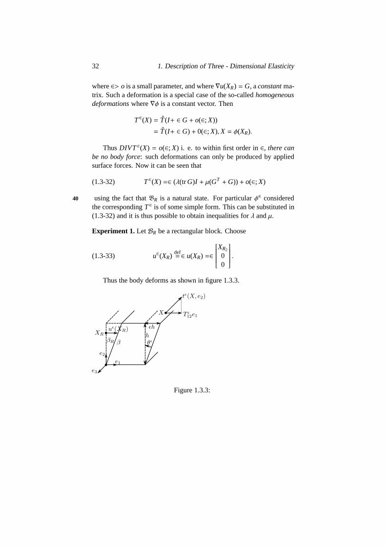
32 1. Description of Three - Dimensional Elasticity
where∈> o is a small parameter, and where∇u(XR) = G, aconstantma-trix. Such a deformation is a special case of the so-calledhomogeneousdeformationswhere∇φ is a constant vector. Then
T∈(X) = T(I+ ∈ G+ o(∈; X))
= T(I+ ∈ G) + 0(∈; X),X = φ(XR).
ThusDIVT∈(X) = o(∈; X) i. e. to within first order in∈, there canbe no body force: such deformations can only be produced by appliedsurface forces. Now it can be seen that
(1.3-32) T∈(X) =∈ (λ(tr G)I + µ(GT +G)) + o(∈; X)
using the fact thatBR is a natural state. For particularφ∈ considered40
the correspondingT∈ is of some simple form. This can be substituted in(1.3-32) and it is thus possible to obtain inequalities forλ andµ.
Experiment 1. LetBR be a rectangular block. Choose
(1.3-33) u∈(XR)def= ∈ u(XR) =∈
XR2
00
.
Thus the body deforms as shown in figure 1.3.3.
Figure 1.3.3:
1.3. Constitutive Equations 33
Then it is logical to assumeT∈12 =∈ T12 + o(∈) whereT12 > o. Thisfollows from the interpretation of the components of the stress tensor(cf. Remark 1.2.2). Comparing this form with (1.3-32) if follows that
(1.3-34) µ > 0.
41
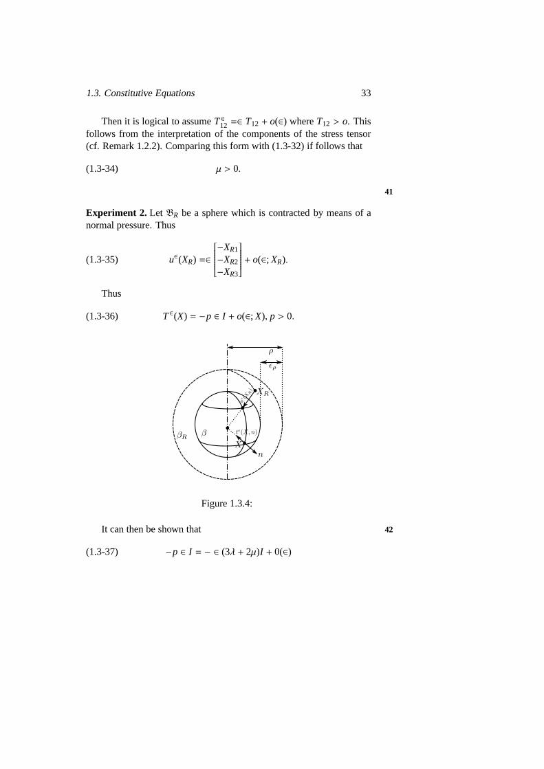
Experiment 2. Let BR be a sphere which is contracted by means of anormal pressure. Thus
(1.3-35) u∈(XR) =∈
−XR1
−XR2
−XR3
+ o(∈; XR).
Thus
(1.3-36) T∈(X) = −p ∈ I + o(∈; X), p > 0.
Figure 1.3.4:
It can then be shown that 42
(1.3-37) −p ∈ I = − ∈ (3λ + 2µ)I + 0(∈)
34 1. Description of Three - Dimensional Elasticity
from which it follows that
(1.3-38) 3λ + 2µ > 0.
Remark 1.3.5.This precludesincompressible materials!An exampleof an incompressible material is rubber.
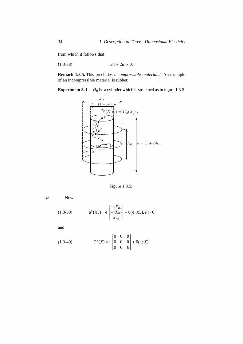
Experiment 3. LetBR be a cylinder which is stretched as in figure 1.3.5.
Figure 1.3.5:
Now43
(1.3-39) u∈(XR) =∈
−νXR1
−νXR2
XR3
+ 0(∈; XR), ν > 0
and
(1.3-40) T∈(X) =∈
0 0 00 0 00 0 E
+ 0(∈; X).

1.3. Constitutive Equations 35
It can now be shown that
(1.3-41) ν =λ
2(λ + µ),E =
µ(3λ + 2µ)λ + µ
Sinceµ > 0 and 3λ + 2µ > 0, it follows thatλ + µ > 0. Sinceν > 0it follows that
(1.3-42) λ > 0.
Thusλ > o andµ > 0. (This does not make sense for incompress-ible materials). The numberν is known asPoisson’s ratioand E asYoung’s modulus. The Lame’s constants can be expressed in terms ofthese quantities:
(1.3-43) λ =Eν
(1+ ν)(1− 2ν), µ =
E2(1+ ν)
.
Thusλ > O andµ > O is equivalent to
(1.3-44) 0< ν < 1/2,E > 0.
(For an incompressible material,ν = 1/2).An elastic material is said to be aSt Venant-Kirchhoff material if 44
(1.3-45) Σ∗R(E) = λ(tr E)I + 2µE.
It is also expressible in terms ofC:
(1.3-46) ΣR(C) =
λ
2(ı1(C) − 3)− µ
I + µC.
Then the Cauchy stress tensor can be written as
(1.3-47) T = T(B) = (ı3(B))1/2
λ
2(ı1(B) − 3)− µ
B+ µ(ı1(B))1/2B2.
Thus such a material is isotropic and material frame indifferent (cf.Theorem 1.3.4).

36 1. Description of Three - Dimensional Elasticity
Remark 1.3.6.While the relation (1.3-45) betweenΣR andE is linear,as a function ofu,ER is non-linearsince the dependence ofE onu non-linear (cf. (1.1-20)).
The relation (1.3-45) can be written componentwise as follows:
ΣRi j = λEkkδi j + 2µEi j
def= ai jkℓEkℓ(1.3-48)
where theelasticity coefficients ai jkℓ are defined by
(1.3-49) ai jkℓ = λδi jδkℓ + 2µδikδ jℓ.
The mappingE→ λ(tr E)I + 2µE is invertible if and only ifµ(3λ +2µ) , o (and we know thatµ(3λ + 2µ) > O from above). Thus givenΣR
there corresponds a uniqueΣ. However, this is not always true in actualexperiments for large deformations. This model can be expected to beacceptable only for small strainsE.
Exercises45
1.3-1. Given a matrixA ∈ S3> show thatA1/2 is uniquely defined inS3
>.If F is an invertible matrix andF = RU = VS,U = (FT F)1/2,V = (FFT )1/2 show thatR = FU−1,S = V−1F are orthogonal.Show also thatS = R, thus proving theorem 1.3.1.
1.3-2. If BR is any reference configuration of an isotropic, materialframe-indifferent material, explain whyΣR(I ) is just a multipleof I as shown in Theorem 1.3.6.
1.3-3. Complete the details in the proof thatλ, µ > O for a naturalstate. In particular, prove relations (1.3-32), (1.3-34),(1.3-37),and (1.3-41).

1.4. Hyperelasticity 37
1.4 Hyperelasticity
If the constitutive equation is taken into account, the equilibrium equa-tions in the reference configuration reduce to a system of three equa-tions, for the three components of the deformationφ, along with bound-ary conditions:
DIVRTR(∇φ) + ρRbR = O in BR(1.4-1)
TR(∇φ)nR = t1R on∂B1R(1.4-2)
φ = φ0 on∂B0R.(1.4-3)
This is equivalent to the variational equations
(1.4-4)∫
BR
TR(∇φ) : ∇θdXR =
∫
BR
ρRbR.θdXR +
∫
∂B1R
t1R.θdAR
for all θ : BR→ R3, vanishing on∂BoR.It was seen in section 1.2 that if the body forces and applied surfaces 46
were conservative, then (1.4-4) could be written in the form
(1.4-5)∫
BR
TR(∇φ) : ∇φdXR = B′(φ)θ + T′1(φ)θ
for real-valued functionalsB andT1 (cf. (1.2-32) and (1.2-35).If it were possible to write
∫
BR
TR(∇φ) : ∇θdXR
asW′(φ)θ for some functionalW, then the problem (1.4-4) would reduceto finding the stationary points of the functionalW− (B+ T1).
Note that upto now, the equations which give the symmetry ofΣR =
(∇φ)−1TR have not been mentioned; it will be seen later (cf. Theorem1.4.3) that for materials under consideration in this section, these equa-tions will automatically be satisfied.
The above considerations lead to the following definition:
38 1. Description of Three - Dimensional Elasticity
A homogeneous elastic material is said to behyperelasticif thereexists a differentiable functionW : M3
+ → R such that
(1.4-6) TR(F) =∂W
∂F(F)
for all F ∈ M3+, or componentwise,
(1.4-7) TRi j (F) =∂W
∂Fi j(F).
A word on notation: theFrechet derivtiveW ′(F) : M3 → R is a47
continuous linear operator such that forF, andF +G inM3+,
W(F +G) =W(F) +W′(F)G + o(G)
=W(F) +∂W∂Fi j
(F)Gi j + o(G).
The term∂W∂Fi j
(F)Gi j will also be written as
∂W∂F
(F) : Gdef=∂W∂Fi j
(F)Gi j ,
where thematrix∂W∂F
(F) has components∂W∂Fi j
(F).
Theorem 1.4.1. Consider a homogeneous hyperlastio material actedon by body and applied surface forces which are conservative. Then theboundary value problem with respect toφ is formally equivalent to
(1.4-8) I ′(φ)θ = 0
for all θ : BR → R3, vanishing on∂BoR where, for allψ : BR→ R3,
(1.4-9) I (ψ) =∫
BR
W(∇ψ(XR))dXR − (B(ψ) + T1(ψ)).
1.4. Hyperelasticity 39
Proof. Givenψ : BR → R3 andW : M3+ → R, let
W(ψ)def=
∫
BR
W(∇φ)dXR.
Then givenψ andθ,
W(ψ + θ) −W(ψ) =∫
BR
(W(∇(Ψθ)(XR)) −W(∇ψ(XR)))dxR
=
∫
BR
[
∂W∂F
(∇ψ(XR)) : ∇θ(XR) + o(|vθ(XR)|; XR)
]
dXR
=
∫
BR
TR(∇ψ) : ∇θdXR + o(||θ||).
Thus, at least formally, 48
(1.4-10) W′(ψ)θ =∫
RTR(∇ψ) : ∇θdXR
and the result follows.
Remark 1.4.1.It must be verified in each circumstance thetW is Frechetdifferentiable and that the right hand side of (1.4-10) does indeed givethe Frechet derivative. If theC1-uniform norm is chosen for the space ofdifferentiable vector functions onBR and if the first partial derivativesof TRi j are Lipschitz Continuous it can be it can be seen that is indeedthe case.
The functionalW is called thestrain energyandI is called thetotalenergy. The functionW : M3
+ → R is called thestored energy function.
Notice that the boundary value problerm is precisely theEuler equa-tions associatedto the total energy.
If φo on∂BoR is extended to the whole ofBR andIo defined by
Io(ψ) = I (ψ + φo)

40 1. Description of Three - Dimensional Elasticity
then one looks forφ − φo vanishing on∂BoR such that
I ′o(φ − φo)θ = o
for all θ : BR → R3 vanishing on∂BoR. Thus particular solutions are49
thoseφ which satisfy
(1.4-11) I (φ) =
inf
ψ : BR→ R3
ψ = φ0 on∂BoR
I (ψ).
In the next chapter, it will be seen that the formulation in terms ofthe boundary value problem will be the basis for proving existence ofsolutions via the implicit function theorem while (1.4-11)will be thebasis for the approach due to J. BALL.
A stored energy functionW : M3+ → R will be said to be mate-
rial frame indifferent (resp isotropic) ifTR =∂W∂F
is material frame
imdifferent (resp. isotropic).Now necessary and sufficient conditions for a stored energy function
to be material frame indifferent or/and isotropic will be examined.
Theorem 1.4.2.The stored energy functionW : M3+ → R is material
frame indifferent if and only if, for all FǫM3+ and for all QǫO3
+
(1.4-12) W(QF) =W(F).
Equivalently, it is material frame indifferent if and only if there existsa functionW : S3
> → R such that for all FǫM3+
(1.4-13) W(F) = W(FTF)
(cf. Equation(1.3-6)).
Proof. Since material frame indifference is equivalent to50
T(QF) = QT(F)QT
1.4. Hyperelasticity 41
for all FǫM3+ and for allQǫO3
+, and since
TR(F) = detFT(F)F−T
it follows that material frame indifference is equivalent to
(1.4-14) TR(QF) = QTR(F)
for all FǫM3+ andQǫO3
+, i.e.,
(1.4-15)∂W∂F
(QF) = Q∂W∂F
(F)
in case of hyperelastic materials. Define
(1.4-16) WQ(F) =W(QF),QǫO3+, FǫM
3+.
Now if F +G ǫ M3+,
WQ(F +G) =W(QF + QG) =∂W∂F
(QF) : QG+ o(QG)
= QT ∂W∂F
(QF) : G+ o(G)
where the relationA : BC = BTC has been used (cf. Remark 1.4.2).Thus
∂WQ
∂F(F) = QT ∂W
∂F(QF).
Thus material frame indifference is equivalent to
(1.4-17)∂
∂F(WQ(F) −W(F)) = 0.
NowM3+ is connected inM3(cf,. Exercise 1.4-2 and so the above is51
equivalent to)
(1.4-18) W(QF) =W(F) +C(Q),
42 1. Description of Three - Dimensional Elasticity
for all FǫM3+,QǫO
3+. SettingF = I ,Q,Q2, . . . successively, it follows
that
W(Q) =W(I ) +C(Q)
W(Q2) =W(Q) +C(Q)
. . . .
Thus fo any integerp ≥ 1,
(1.4-19) W(QP) =W(I ) + pC(Q).
Then|W(QP)| ≥ p|C(Q)| − |W(I )|.
Thus ifC(Q) , 0, then|W(QP)| → +∞ asp→ ∞. But the setO3+
is compact inM3+ andW is continuous since it is differentiable. Hence
C(Q) = 0 and the first assertion is proved.To prove the second equivalence, letF = RU be the polar factoriza-
tion of F (cf. Theorem 1.3.1). ForCǫS3>, set
(1.4-20) W(C) =W(C1/2).
Then
W(F) =W(RU) =W(U) = W(U2) = W(FTF)
sinceU2 = FTF. Conversely, if (1.4-13) is true, then forFǫM3+ and52
QǫO3+,
W(QF) = W(FTQTQF) = W(FT F) =W(F).
It can be show that (cf. Exercise 1.4-4) ifW is differentiable, so is
W. Without loss of generality, it may be assumed that the matrix∂W∂C
is symetric. For
W(C) = W(C +CT
2),CǫS3
>.
1.4. Hyperelasticity 43
Remark 1.4.2.The following identities involving the scalar product : inM
3 are useful.
A : BC = tr(ACT BT) = tr(BT−ACT) = BTA : C(1.4-21)
A : BC = ACT : B = B : ACT = tr(BCAT) = tr(CATB) = CAT : BT .
(1.4-22)
The identity (1.4-21) was used in the proof of the above theorem.
The following theorem says that in case of frame indifferent hy-perelastic materials, the symmetry of the second Piola-Kirchhoff stresstensor is automatically verified.
Theorem 1.4.3. Let the material be hyperelastic and material frameindifferent. Then
(1.4-23) ΣR = ΣR(F) = ΣR(FT F) = 2∂W∂C
(C),C = FTF.
Thus the second Piola-Kirchhoff stress tensor is automatically sym-metric. Conversely, if there exists a mappingW : S3
> → R such that
(1.4-24) ΣR(F) = 2∂W∂C
(FTF)
then the material is hyperelastic with 53
(1.4-25) W(F) = W(FTF)
and consequently is material frame indifferent.
Proof. ΣR(F) = F−1TR(F) = F−1∂W∂F
(F).
AlsoW(F) = W(FT F). Now if F, F +GǫM3+,
W(F +G) −W(F) = W(FTF + FTG+GTF +GTG) − W(FTF)
=∂W∂C
(FT F) : (FTG+GTF) + o(G)
= F∂W∂C
(FT F) : G+ F(∂W∂C
(FT F))T : G+ o(G)
44 1. Description of Three - Dimensional Elasticity
by (1.4-21) - (1.4-22). But∂W∂C
is symmetric. Thus
W(F +G) −W(F) = 2F(∂W∂C
(FT F)) : G+ o(G).
Hence54
∂W∂F
(F) = 2F∂W∂C
(FTF)
or ΣR(F) = F−1∂W∂F
(F) = 2∂W∂C
(FTF).
Conversely, ifW(F) = W(FT F) then consider the mappingF →FTF fromM3
+ into S3+. One has
W′(F)G = W′(FTF)(FTG+GTF)
or
∂W∂F
(F) : G =∂W∂C
(FTF) : (FTG+GTF)
= 2F∂W∂C
(FT F) : G as before.
Hence∂W∂F
(F) = FΣR(F) = TR(F)
and the result follows.
Now the effect of isotropy on a stored energy function can be simi-larly examined.
Theorem 1.4.4.A stored energy functionW : M3+ → R is isotropic if,
and only if, for every FǫM3+ and for every QǫO3
+,
(1.4-26) W(F) =W(FQ).
Proof. The argument runs along the same lines of that of Theorem 1.4.2and is left as an exercise (cf. Exercise 1.4-5).

1.4. Hyperelasticity 45
Theorem 1.4.5. A stored energy functionW : M3+ → R is material
frame indiffernt and isotropic if, and only if, there exists a function
φ = ( ]0,+∞[ )3→ Rsuch that W(F) = φ(ıFT F) = φ(ıFFT ) (1.4− 27)
for every FǫM3+.
Proof. By the material frame indifference, there exists a functionW :S
3> → R such that
W(F) = W(FT F).
By the isotropy, ifQǫO3+, then
W(F) =W(FQ) = W(QT FTFQ).
55
ThusW : S3> → R satisfies
W(C) = W(QTCQ)
for every C ǫ S3> and for everyQ ǫ O3
+ (since for everyCǫS3> there
correspondsF = C1/2ǫ M3+ with C = FTF). Now it was shown in
the proof of the Rivlin-Ericksen Theorem (Theorem 1.3.4) that such afunction must be a function of the principal invariants
Cnversely, ifW(F) = φ(1FT F), let QǫO3+.
Then
ı(FQ)T FQ = ıQT FT FQ = ıFT F
ı(QF)T QF = ıFT F
and soW(F) =W(QF) =W(FQ)
and the thoerem is proved.
The next result expresses the Piola-Kirchhoff stress tensors in termsof the functionφ of the above theorem.
46 1. Description of Three - Dimensional Elasticity
Theorem 1.4.6. Given a functionφ : (]0,+∞[)3 → R and a storedenergy function
W(F) = φ(ı1(C), ı2(C), ı3(C)),C = FT F,
then
(1.4-28)12
TR(F) =∂φ
∂ı1F +
∂φ
∂ı2(ı1I − FFTF) +
∂φ
∂ı3ı3F−T
where56
ık = ık(FTF) and
∂φ
∂ık=∂φ
∂ık(ıFT F), k = 1, 2, 3.
Furthere
12ΣR(C) =
∂φ
∂ı1I +
∂φ
∂ı2(ı1I −C) +
∂φ
∂ı3ı3C−1(1.4-29)
=
(
∂φ
∂ı1+∂φ
∂ı2ı1 +
∂φ
∂ı3ı2
)
I
−(
∂φ
∂ı2+∂φ
∂ı3ı1
)
C +∂φ
∂ı3C2.
Proof. Let Γ be the mapΓ : M3+ → S3
> given byΓ(F) = FTF. Now
TR(F) =∂W∂F
(F) where
∂W∂F
(F) : G =∂φ
∂ık(ıC)Γ′(F)G.
Now ı1(C) = tr C and so
ı1′(C)D = tr(D),(1.4-30)
ı3(C) =16
[
3(trC)3 − 3(trC) tr(C2) + 2 tr(C3)]
and so
ı′3(C)D =16
[
3(trC)2(tr D) − 3(tr D) tr(C2) − 6(trC) tr(CD) + 6 tr(C2D)]

1.4. Hyperelasticity 47
=12
[
(tr C)2 − tr(C2)]
tr(D) + tr(C2D) − tr(C) tr(CD)
= ı2(C) tr(D) + tr(C2D) − tr(C) tr(CD).
Now
tr(C2D) − tr(C) tr(CD) = tr((C2 − ı1(C)C)D)
= tr(ı3(C)C−1D − ı2D
using the Cayley-Hamilton theorem. Thus 57
(1.4-31) ı3′(C)D = ı3(C) tr(C−1D).
Finally
ı2(C) =12
[
(tr C)2 − tr(C2)]
ı2′(C)D = tr(C) tr D − tr(CD)
= tr((ı1(C)I −C)D)
= tr((ı2(C)C−1 − ı3(C)C2)D)
again using the Cayley-Hamilton theorem. This may be again written as
(1.4-32) ı2′(C)D = ı3(C) tr(C=1) tr(C−1D) − ı3(C) tr(C−2D).
Also, Γ′(F)G = FTG+GTF. Thus’
∂W∂F
(F) : G =∂φ
∂ı1tr(FTG+GTF)
+∂φ
∂i2i3 tr(C−1) tr(C−1(FTG+GTF))
+∂φ
∂i2i3 tr(C−2)(FTG+GTF))
+∂φ
∂i2i3 tr(C−1)(FTG+GTF))
Now, tr(FTG+GTF) = 2F : G
tr(C−1(FTG+GTF)) = C−T : (FTG+GTF)

48 1. Description of Three - Dimensional Elasticity
= F−1F−T : (FTG+GTF)
= 2F−T : G(Using(1.4-21)− −(1.4-22))
tr(C−2(FTG+GTF)) = C−2T : (FTG+GTF)
= C−2 : (FTG+GTF)
= F−1F−TF−1F−T : (FTG+GTF)
= 2F−T F−1FT : G
58
Hence
12∂W∂F
(F) : G =∂Φ
∂ı1ı3 tr(C−1)F−T : G
− ∂Φ∂ı2
ı3F−T F−1F−T : G+∂Φ
∂ı3ı3F−T : G
Now, consider
ı3 tr (C−1)F−1 − ı3F−TF−1F−T
= ı3[
tr(C−1)F−T F−1 − F−TF−1F−TF−1]
F
= ı3[
tr(B−1)B−1 − B−2]
F, B = FFT
= (ı2B−1 − ı3B−2)F
since B and C are similar. Againık = ık(B). Now by the Cayley-Hamilton theorem,
ı2B−1 − ı3B−2 = ı1I − B = ı1I − FFT .
Combining all these relation (1.4-28) follows. To obtain (1.4-29)note that ˆ
∑
R(F) = F−1TR(F). Hence
12ΣR(F) =
∂Φ
∂ı1I +
∂Φ
∂ı2(ı1I − FT F) +
∂Φ
∂ı3ı3F−1F−T
which gives the first relation. To get the second, by the Cayley- Hamil-ton theorem,
ı3C−1 = C2 − ı1C + ı2I
and the result follows. 59
1.4. Hyperelasticity 49
Remark 1.4.3.Compare the last relation in (1.4-29) with the statementof Rivlin- Ericksen theorem (Theorem 1.3.4)
Theorem 1.4.7.Consider a St venant- Kirohhoff material with
(1.4-33) Σ∗R(E) = λ tr (E) + 2µE
It is hyperlastic with
W∗ (E) =λ
2(tr E)2 + µ tr(E2)(1.4-34)
=(λ + 2µ)
8(ı1 − 3)2 + µ(ı1 − 3)− µ
2(ı2 − 3) = Φ(ıC)
whereık = ık(C), k = 1, 2, 3.
Proof. SetW(C) =W(I + 2E) =W∗ (E).
Now
W∗ (E + H) =W∗ (E) + λ tr E tr H + 2µ tr (EH) + o(H)
=W∗ (E) + (λ(tr E)I + 2µE) : H + o(H).
Hence∂W∗∂E
(E) =∗
∑
R
(E).
This implies that
˜∑
R(C) = 2
∂W∂C
(C)
and hence the material is hyperelastic. The verification of the expressionfor Φ is left as an exercise to the reader.
Remark 1.4.4.The above result gives another proof (cf. equation60
(1.3-47)) that St Venat-Kirchhoff materials are isotropic and materialframe indifferent.

50 1. Description of Three - Dimensional Elasticity
Remark 1.4.5.Other examples of hyperelastic materials will be seen inChapter 2 (Ogden’s materials)
Theorem 1.4.8.LetBR be a natural state of a material which is isotro-pic and material frame indiffrent. Then ifWǫC1(M3
+; R)
(1.4-35) W∗ (E) =λ
2(tr E)2 + µ tr(E2) + o(|E|2).
Proof. Let
W∗ (E) =λ
2(tr(E))2 + µ tr(E2) + δW∗ (E)
∂W∗∂E
E = λ(tr E)I + 2µE +∂δW∗∂E
(E)
= Σ∗R(E) = λ tr E) + 2µE + o(E).
Thus,∂δW∗∂E
(E) = o(E).
Since subtracting a constant inW∗ does not change the stress ten-sors, it can be assumed, without loss of generaliry, thatδW ∗ (o) = o.Hence
δW∗)(E) =
1∫
0
∂δW∗∂E
(E) : dt = o(|E|2).
Exercises61
1.4-1 For a non-homogeneous hyperelastic material,
TR(XR, F) =∂W∂F
(XR, F)
for everyXRǫBR, and for everyFǫM3+. Extend the analyisi of this
section to such materials.

1.4. Hyperelasticity 51
1.4-2 (i) Show thatM3+ is a connected subset ofM3.
(ii) Show by an example thatM3+ is not convex.
(iii) Identify its convex hull inM3.
1.4-3 Assume that (cf. Proof of Theorem 1.4.2)
W(QF) =W(F) +C(Q)
For all FǫM3+ and QǫO3
+. Show thatC(Q) = o without using thecontinuity ofW.
1.4-4 (i) Show thatS3> is an open subset ofS3.
(ii) Show that ifW is differentiable, so isW.
1.4-5 Prove Theorem 1.4.4: show that isotropy is equivalent to
TR(FQ) = TR(F)Qfor allFǫM3+
andQǫO3+, which is in turn equivalent to
∂W∂F
(F) =∂W∂F
(FQ)QT =∂W∂F
(F),W(FQ).(FQ).
1.4-6 Check the second relation in equation (1.4-34).
1.4-7 Consider an elastic matrial with
T(B) = Bo(ıB)I + B1(ıB)B+ B2(ıB)B2.
Find necessary and sufficient conditions on 62
βα : (]o,+∞[)3 → R, α = 0, 1, 2
for the material to be hyperelastic.
1.4-8 In Theorem 1.4.8, compute the terms of order 2 in∑∗
R(E) andterms of order 3 inW∗(E). Explain the discrepancy in the numberof terms obtained in each case.
52 1. Description of Three - Dimensional Elasticity

Chapter 2
Some Mathematical Aspectsof Three-DimensionalElasticity
63IN THIS CHAPTER, questions of existence of solutions to the bound-ary value of three-dimensional elasticity will be examined. In the firstsection, some general considerations about these boundaryvalue prob-lems will be mentioned. The problems will be classified with respectto boundary conditions. As good models of elasticity must precludeuniqueness of solution, several examples of non-uniqueness will be pre-sented.
The first tool for the study of existence of solutions is the implicitfunction theorem. As this requires a knowledge of the linearized prob-lem, the second section will briefly present linear elasticity and the thirdsection will prove existence, albeit for a very narrow classof boundaryconditions. The fourth section will study incremental methods, whoseanalysis follows closely related lines.
The last two sections will present results on polyconvexityand ex-istence of solutions to the problem of minimizing the energyusing theapproach of J. BALL. Though several types of boundary conditions canbe studied here, the main drawback is the lack of regularity of solutionsand so it is not known if the solutions satisfy the equilibrium equations.
53
54 2. Some Mathematical Aspects of Three-Dimensional.....
2.1 General Considerations About the BoundaryValue Problems of Three-Dimensional Elasticity
64Given a respones functionTR : M3
+ → M3 satisfying
(2.1-1) F(TR(F))T = TR(F)FT
for every FǫM3+ and given the denstiyρR : BR → R and dead loads
bR : BR→ R3, ıR : ∂B1R→ R3, the boundary value problem arising outof the equilibrium equations amounts to finding a deformation Φ whichsatisfies
DIVRTR(∇φ) + ρRbR = 0 inBR(2.1-2)
TR(∇φ)nR = t1R on∂B1R(2.1-3)
φ = φo (given) on∂BoR(2.1-4)
The boundary conditionφ = φo on ∂BoR is called aboundary con-dition of place. The boundary condition (2.1-3) on∂B1R is called aboundary condition of traction(and this defnition implies it is a deadload).
If ∂BoR = φ the problem is apure tractionboundary value prob-lem.If ∂B1R the problem is apure displacementproblem. If both∂BoR
and ∂B1R have strictly positivedAR- measure, then the problem is amixed displacement-tranctionproblem.
Recall that
ˆ∑
R(∇φ) = (∇φ)−1TR(∇Φ)
whereˆ∑
R: M3+ → S3
and the boundary value problem (2.1-2)–(2.1-4) can be rewritten in65
terms of this tensor. If the material is hyperelastic (cf. Section 1.4), then
(2.1-5) TR(F) =∂W∂F
(F)
2.1. General Considerations. . . 55
for a stored energy functionW : M3+ → R and the problem is equivalent
to finding the sationary points of an energy functional,
(2.1-6) I (ψ) =∫
BR
W(∇ψ)dXR −
∫
BR
ρRbR.ψdXR +
∫
∂B1R
t1R.ψdAR
The partial differentail equations (2.1-2) are nonliner with respect toφ since the mappingTR : M3
+ → M3 is non-linear, and of the secondorder. The non-linearity occurs in the highest order terms and this is asource of difficulty. Another source of difficulty is that the solutionφmust satisfy det (∇φ) > o. Thus for instance in (2.1-6)ψ must vary overM
3+ which is clearly not a vector sapce; in fact it is not even a convex
subset ofM3 (cf. Exercise 1.4-2).The boundary condition of traction could be replaced by the so-
called boundary condition of pressure(which is not a dead load, butit is conservative). Again it is possible to have apure pressurebound-ary value problem (for instance, a soap bubble or a submarine) or mixeddisplacement-pressureboundary value problems.
These boundary condition, though being the only ones to be con-sidered here, are far from exhaustive. Other types of conditions arepossible.
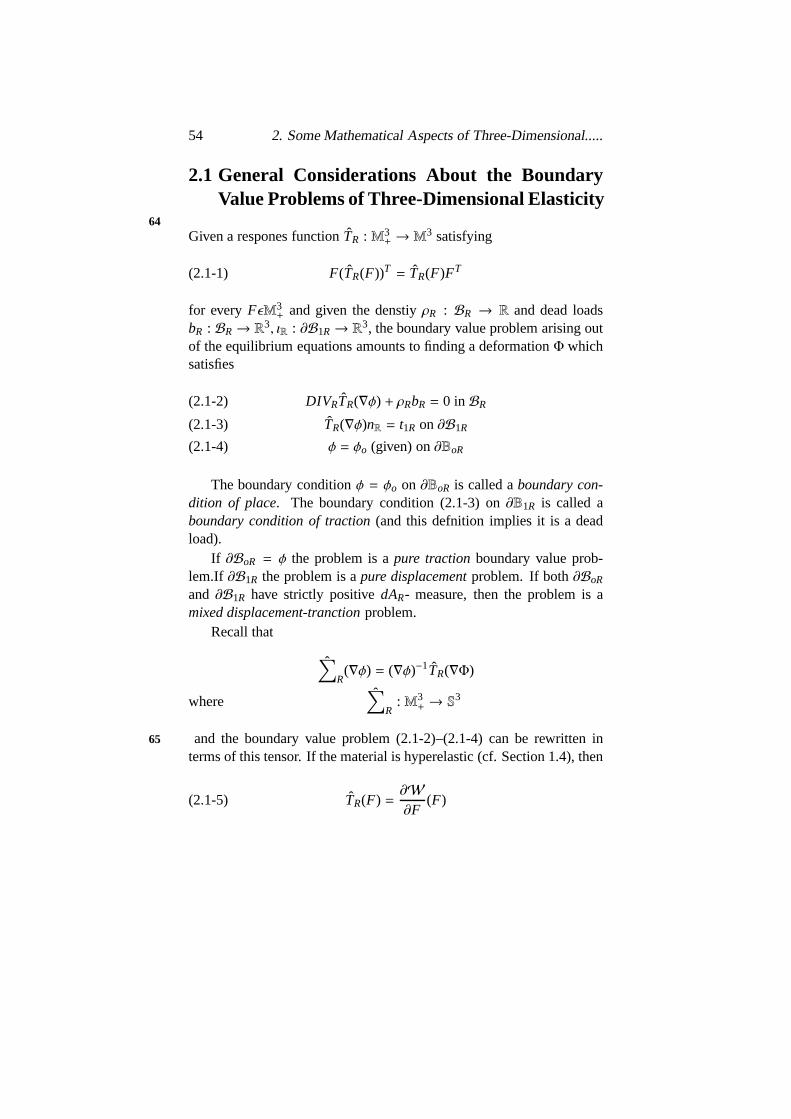
In practice one can haveunilateral conditions. For instance, if the 66
body must remain in above the plane spanned bye1, e2 the boundarycondition isX3 ≥ o or φ3(XR) ≥ o
Figure 2.1.1:
It is also possible to have a mixture of displacement and stress boun-dary conditions. ConsiderBR to be a plate with a pressurep compress-

56 2. Some Mathematical Aspects of Three-Dimensional.....
ing the lateral surface (fig 2.1.2) and given only by itshorizantal aver-age. Then the conditions are
(2.1-7)
u1, u2independent ofX3
u3 = 0
and
(2.1-8)12ǫ
ǫ∫
−ǫ
T(∇φ(XR)n dX3 = −pn.
Figure 2.1.2:67
Apart from possibly the problem of bodies moving with constantvelocity in a fluid, the pure traction problems are less common. Thepure displacement problems are quite unrealistic.
In general, several deformed states are possible for the same sys-tem of forces, though they may not all be physically feasibleor ‘sta-ble’. Nevertheless the mathematical model cannot recognize the feasi-ble or stable ones. Hence a good model will always account fornon-uniqueness of solutions. Several examlpes of non-uniqueness will nowbe given .
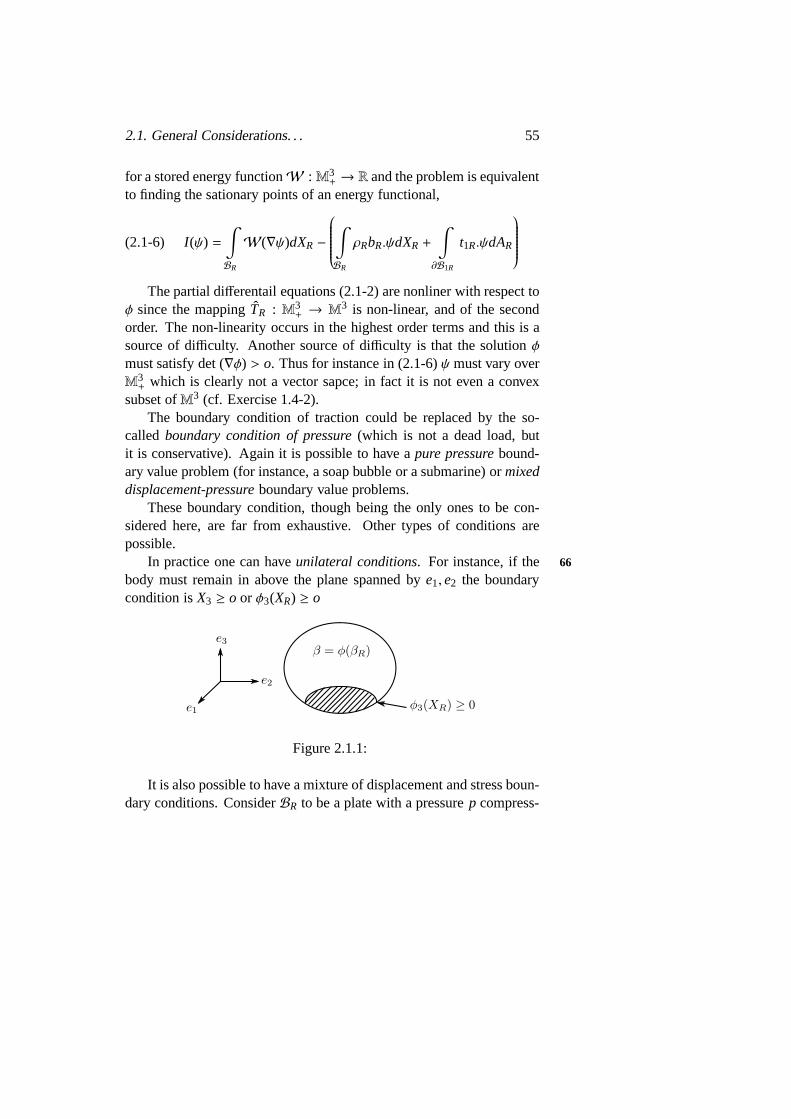
Example 2.1.1.A mixed displacement-traction problem. Consider along circular cylinder fixed at either end. The body force is just itsweight. On the lateral surfacet1R = o. Assume the body to be ex-tremely pliable, and rotate one end by an angle of 2π and reglue it in itsoriginal position. Then a line parallel to the axis on the lateral surface
2.1. General Considerations. . . 57
will deform into a curve and thus gives another solution other than the68
natural one, which will just be a slight bending of the cylinder underits weight. It is theoretically possible to rotate the face by 2kπ for anypositive integerk. Thus the model must account for an infinite numberof solutions.
Figure 2.1.3:
Example 2.1.2(F. JHON). A pure displacement problem. Consider thebody to be betwen two concentric spheres. Assumeu ≡ 0 on both theinner and outer surfaces. Apart from the trivial solution, it is possible tohave an infinite number of solutions by (theoretically) rotating the innersphere about an axis by an angle of 2kπ and re-glueing it to the body.
Figure 2.1.4:
69
58 2. Some Mathematical Aspects of Three-Dimensional.....
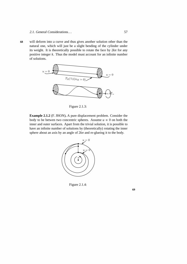
Example 2.1.3(C. ERICKSEN). A pure traction problem.A rectangularlock is pulled normal to the upper and lower surfaces. Rotation of theconfiguration byπ produces a (though urrealistic) solution where thebody is comprssed!
Figure 2.1.5:
Example 2.1.4.Consider a thin circular plate subjected to the boundary70
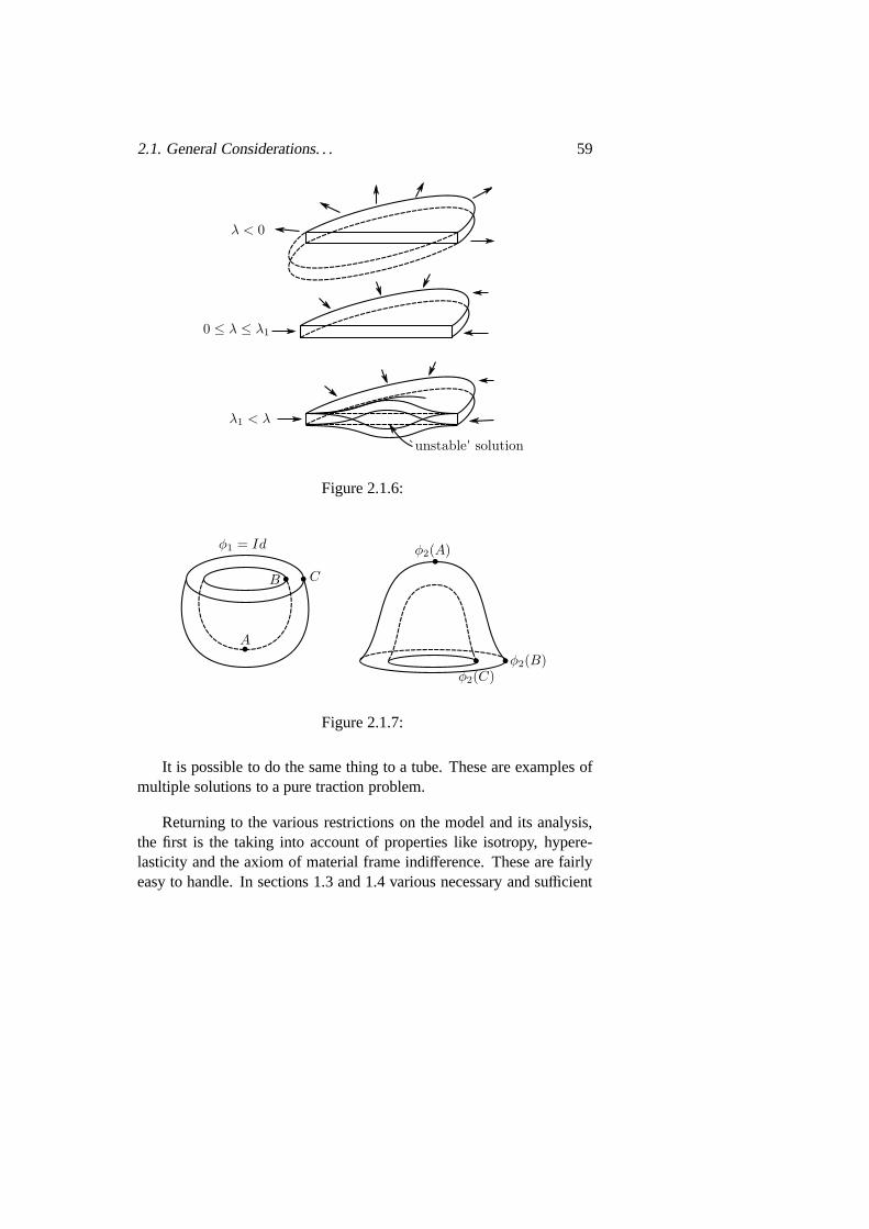
condition (2.1-7) - (2.1-8) withp = λp1. If λ < 0 (i.e the plate is pulled)or if λ > o and small,u ≡ o is the only possible solution. Ifλ exceedsa critical value, the plate can buckle upwards or downwards thus givingtwo additional solutions (cf. 2.1.6) This is a buckling phenomenon
Example 2.1.5.Eversion problems. A cut tennis ball (borrowed from avery good friend) can be made to exist in two diffrent states as shown infig 2.1.7. The everted state can be produced by pushing hard enough on71
the natural state.
2.1. General Considerations. . . 59
`unstable' solution
Figure 2.1.6:
Figure 2.1.7:
It is possible to do the same thing to a tube. These are examples ofmultiple solutions to a pure traction problem.
Returning to the various restrictions on the model and its analysis,the first is the taking into account of properties like isotropy, hypere-lasticity and the axiom of material frame indifference. These are fairlyeasy to handle. In sections 1.3 and 1.4 various necessary andsufficient

60 2. Some Mathematical Aspects of Three-Dimensional.....
conditions of the relevant functions were studied. The mainrestrictionis that the solutionφ must satisfy forces
det(∇φ) > o.
In using the implicit function theorem, this requirement isignoredat first and then shown to be satisfied for sufficiently small forces.
In the different approach of J. BALL, this is taken into account (a.e72
in BR) by imposing it on the setU of test functions over which theenergy is minimized. This precludes the convexity ofU which makesminimization more difficult than usual. In this approach, it will be nicelytaken into account by imposing thatW(F) → +∞ when det (F)→ o+.
Even if det∇φ > o everywhere onBR, it does not ensure thatφ is aone-one mapping, a property natural to expect in a deformation.Thus ifa body as in fig. 2.1.8(a) in contact with the horizontal planeis pushedalong the two ‘arms’, it must take a shape as in fig 2.1.8(b). But themathematical model will not preclude a situation as in fig 2.1.8(c) wherethe material penetrates itself, still keeping det∇φ > 0
(a) (b) (c)
Figure 2.1.8:
In the case of incompressible materials, the energy is minimized73
over a set of functionψ (in a suitable function space) with
det(∇ψ) = 1 a.e.
Some of the noations used hitherto will be changed.BR will hence-forth be denoted byΩ,Ω a bounded open subset ofR3 and its boundary∂BR by Γ. The portions∂BoRand∂B1R will be denoted byΓo andΓ1
respectively.

2.1. General Considerations. . . 61
The generic pointXR will henceforth be labelledx anddXR anddAR
will be changed todx andda respectively. The derivatives∂
∂XRiwill
be denoted by∂i andDIVR by div. The normalnR to ∂BR will now begiven byv = (vi), the unit outer normal toΓ.
The tensors∑
R= (
∑
Ri j
) andTR = (TRi j ) will be denoted by (σi j ) and
(ti j ) respectively. The vectorsρRbR andt1R will be denoted byf = ( fi)andg = (gi) respectively. The symbols forφ, u, F = ∇φ, B = FFT ,C =
FT andE =12
(C − I ) will remain unchanged.
Thus, for instance the equations of equilibrium im terms of∑
R readin the old natation as:
DIVR
∇φ∑
R
+ σRbR = o in BR(2.1-9)
∇φ∑
R
nR = t1R on∂B1R(2.1-10)
φ = φ0 on∂B0R(2.1-11)
These, when translated in to the new notations will read as 74
−∂ j(σk j∂kφi) = fi in Ω(2.1-12)
σk j∂kφiv j = gi onΓ1(2.1-13)
φi = φ0i onΓ0(2.1-14)
Exercises
2.1-1 . Assume that a pure traction problem has a solutionφ. Show that∫
BR
ρRbRdXR+
∫
∂BR
t1RdAR = 0
and∫
BR
φΛρRbRdXR+
∫
∂BR
φΛt1RdAR = 0.
62 2. Some Mathematical Aspects of Three-Dimensional.....
2.1-2 .Consider a hyperelastic incompressible material. In the con-strained minimization problem
infψǫU
I (ψ)
where U = ψ | det(∇ψ) = 1a.e.,
show by a formal computation that the Lagrange multiplier isthepressure.
2.2 The Linearized System of Elasticity75
Consider the boundary value problem (2.1-12)-(2.1-14). Interms of thedisplacementu it can be rewritten as
−∂ j(σi j + σk j∂kui) = fi in Ω,(2.2-1)
(σi j + σk j∂kui)v j = gi onΓ1,(2.2-2)
ui = uoi onΓo,(2.2-3)
with the constitutive equation
(2.2-4) σi j = σ∗i j (E(u)) = λEkk(u)δi j + 2µEi j (u) + o(E)
where
(2.2-5) E(u) =12
(
∇uT + ∇u+ ∇uT∇u)
If u were defined in a suitable function space, whose functions van-ish onΓ0, then symbolically one can write
(2.2-6) A(u) =
[
fg
]
The linearised system of elasticity will then be formally defined as(assumingA is differentiable)
A′(0)u =
[
fg
]

2.2. The Linearized System of Elasticity 63
This can be derived as follows. The linearized strain tensoris
(2.2-7) ǫ(u) =12
(
∇uT + ∇u)
.
Thenσ will in turn be linearized as
(2.2-8) σi j = λǫkk(u)δi j + 2µǫi j (u).
76
Substituting this in (2.2-1)-(2.2-3) and keeping only the first orderterms, the linearized syatem elasticity turns out to be
−∂ jσi j = fi in Ω(2.2-9)
σi j v j = gi onΓ1(2.2-10)
ui = uoi onΓ0(2.2-11)
whereσ is given by (2.2-8). Note that such a syatem cannot be a modelfor elasticity (of Exercise 2.2-1) but only approximation of a model.
Remark 2.2.1.If the equations were written in terms ofti j and thenlinearized, the same linearized system of elasticity wouldhave been ob-tained. This is becauseTR = (I + ∇u)
∑
Rand on linearizing this realtion
only the part coming fromI∑
R=
∑
Rwill be retained.
Before the existence and regularity of solution to the linearized sys-tem of elasticity can be studied the following notations forthe Sobolevspaces will be needed.
Let m≥ 0 be an integer and 1≤ p ≤ +∞. Then
(2.2-12) Wm,p(Ω) = vǫLp(Ω) | ∂αvǫLp(Ω)for all | α |≤ m
whereα is a multi-index and∂αv is the corresponding partial derivative( in the sense of distribution). This space is a Banach space with thenorm
(2.2-13) || v ||m,p.Ω=
∫
Ω
∑
|α|≤m
| ∂αv |p dx
1/p
64 2. Some Mathematical Aspects of Three-Dimensional.....
(with the standrad modification ifp = +∞). The semi-norm| . |m,p,Ω is 77
defined by
(2.2-14) || v ||m,p.Ω=
∫
Ω
∑
|α|=m
| ∂αv |p dx
1/p
If m = 0,W0,p(Ω) = Lp(Ω)and | . |0,p,Ω is the usualLp(Ω)- norm.If D(Ω) is the space ofC∞ functions with compact support inΩ, itsclosure inWm,p(Ω) will be denoted byWm,p
o (Ω).If p = 2, it is customary to writeHm(Ω)andHm
0 (Ω) instead ofWm,
2(Ω) andWm,20 (Ω) respectively. The norms and semi-norms in this case
will be written as|| · ||m,Ω respectively| · |m,Ω is theL2(Ω)- norm.By Poincares inequality,| · |m,p,Ω is a norm onWm.p
0 (Ω) and is equiv-alent to|| . ||m,pΩ, for1 ≤ p < ∞.
In case of vector valued or tensor valued functions, the symbolsWm,p(Ω), LP(Ω) will be used to denote that each component is inWm,p
(Ω) or Lp(Ω) respectively. However the symbols for the norms and semi-norms will not be altered.
The following result is fundamental.
Theorem 2.2.1(Korn’s Inequality). LetΓ be smooth enough. Then
(2.2-15) v = (vi)ǫC2(Ω) | ǫi j (v)ǫL2(Ω), 1 ≤ i, j ≤ 3 = H1(Ω)
Consequently, there exists constans C1 > 0andC2 > 0 such that78
(2.2-16)C1 || v ||1,Ω≤ (| v |20,Ω + | ǫ(v) |20,Ω)1/2 ≤ C2 || v ||1,Ω for allvǫH1(Ω).
Proof. See DUVAUT and LIONS [1972] or NITSCHE [1981]. Themain difficulty is in proving (2.2-15). Since the second inquality of(2.2-16) is obvious, the first follows from (2.2-15) and the closed graphtheorem.
A consequence of the above result is
Theorem 2.2.2.LetV be defined by
(2.2-17) V = vǫH1(Ω) | v = 0 onΓ0

2.2. The Linearized System of Elasticity 65
where the da-measure ofΓ0 is strictly positive. Then the semi-norm| ǫ(v) |0,Ω is a norm on V equivalent to the norm|| . ||1,Ω.
Proof. Cf. Exercise 2.2-2.
Assume now thatu = 0 onΓ0. Let V be as in (2.2-17). Multiplying(2.2-9) by a functionvǫV, integration by parts using Green’s formula,and using (2.2-10), (2.2-11) and the symmetry ofσ, the following vari-ational formulation of the problem (2.2-9) - (2.2-11) can beobtained.
FinduǫV such that, for allvǫV,
(2.2-18) a(u, v) = L(v)
where
(2.2-19) a(u, v) =∫
Ω
(λǫkk(u)ǫℓℓ(v) + 2µǫi j (u)ǫi j (v)) dx
and
(2.2-20) L(v) =∫
Ω
fividX+∫
Γ1
givi da.
79
By a simple application of Schwarz’s inequality, it followsthata(., .)is a continuous bilinear form onH1(Ω) andL is a continuous functionalonH1(Ω) (and hence onV as well).
The following existence result holds.
Theorem 2.2.3. Consider the variatiational formulation of the linea-rized syatem of elasticity,(2.2-18), or, equivalently, the problem: FinduǫV such that
(2.2-21) J(u) = infvǫV
J(v)
where
(2.2-22) J(v) =12
a(v, v) − L(v)
if λ > 0 andµ > 0 then the problem has a unique solution.

66 2. Some Mathematical Aspects of Three-Dimensional.....
Proof. Observe that by Theorem 2.2.2 for allvǫV,
(2.2-23) a(v, v) ≥ 2µ | ǫ(v) |20,Ω≥ α || v ||21,Ω
whereα > o (usingλ > o andµ > o). ThusJ : V → R is a convex, andcontinuous functional. Hence it is weakly lower semi continuous. Letuk be a minimizing sequence inV, i.e.
J(uk)→ infvǫV
J(v) < +∞.
SinceJ is coercive (i.e.,J(v)→ ∞as|| v ||→ ±∞) it follows thatukis a bounded sequence and hence has a weakly convergent subsequence.80
Let u be the weakly limit of the subsequence (again indexed byk forconvenience). Then by the weak lower semi-continuity ofJ.
infvǫV
J(v) ≤ J(u) ≤ limk
inf→∞
J(uk) = infv∈V
J(v).
Thus J attains its mimimum atu. It is easy to see that equations(2.2-18) are simply equivalent to the equationJ′(u) = 0. Hence theequivalencve of the two problems sinceJ is convex and the existence ofa solution.
If u1 andu2 are solutions inV thena(u1 − u2, v) = 0 for all vǫV.Settingv = u1 − u2 and using (2.2-23), it follows thatu1 = u2, thusproving the uniqueness of the solution.
Remark 2.2.2.The existence of a unique solution to (2.2-18) also fol-lows directly from (2.2-23) by applying theLax-Milgram Lemma.
Finally, let us state the result on the regularity of solutions to theabove problem.
Theorem 2.2.4. SupposeΓ is smooth enough and for some p≥ 2,f ǫCp(Ω). AssumeΓ1 = φ. Then the solution uǫV = Hı0(Ω) of the corre-sponding linearized system of elasticity is in the spaceVp(Ω), where
(2.2-24) Vp(Ω) = vǫW2,p(Ω) | v = 0 onΓ.
2.2. The Linearized System of Elasticity 67
Proof. The casep = 2 has been proved by NECAS [1967]. If p > 2,the argument goes as follows. LetA′(0) : Vp(Ω) → C
p(Ω) repre-sent the operator of the linearized system of elasticity. Then, if in-
dex (A′(0))def= dim(kerA′(0)) − dim(CokerA′(0)), it was proved by
GEYMONAT [1965] that for all p, 1 < p < ∞, the index was inde- 81
pendent ofp. Now, by the result of Necas above ifp = 2,A′(0) isonto and so dim(Coker(A′(o)) = 0. By uniqueness of the solution,dim(ker(A′(0)) = 0 for all p ≥ 2. Hence the index is zero for allpand so dim(Coker(A′(o))) = 0 for all p ≥ 2, i.e., A′(0) is onto for allp ≥ 2, which proves the theorem.
Remark 2.2.3.The above result does not follow from those of AG-MON, DOUGLIS and NIRENBERG [1964]. Their results state thatiff ǫLp(Ω) implise uǫW2,p(Ω) then f ǫWm,p(Ω) implies uǫW2+m,p(Ω) forour problem. The ’starting’ regularity result (m = 0) needs be know apriori and Theorem 2.2.4 proves that in case of the linearized syatem ofelasticity.
Caution! TheW2,p regularity does not hold for the mixed displace-ment-traction linearized syatem of elasticity.
Exercises
2.2-1 Show that ifǫ(u) =12
(∇uT + ∇u), then a constitutive equation
of the formσ = σ∗(ǫ), with σ∗ a linear function ofǫ, does notsatisfy the axion of material frame indenfference.
2.2-2 Prove Theorem 2.2− 2. (Show first that|ǫ(v)|0Ω) is a norm onV.Prove the equivalence of norms by contradiction: assume thereexists a sequencevkǫV with ||vk||1,Ω = 1 and|ǫ(vk)|0,Ω → 0.
2.2-3 Consider the linearized system of elasticity in variational formwith Γ0 = φ. Show that there exists a solution to the problemprovided
∫
Ω
f dx=∫
Γ
dx,

68 2. Some Mathematical Aspects of Three-Dimensional.....
in the quotient spaceH1(Ω)W, where82
W = vǫH1(Ω) | ǫ(v) = 0.
Show also that
W = vǫ|H1(Ω)|v = a+ bΛ ox.
2.2-4 Extend the regularity result to the case 1< p < 2.
2.2-5 Show that ifµ > 0, there exists aλ0 < 0 such that ifλ0 < λ ≤ 0,the linear forma(., .) given by (2.2-19) is coercive.
2.3 Existence Theorems via Implicit Function The-orem
In this section, existence solutions to thepure displacement problemwillbe proved using the implict function theorem.
For simplicity, consider first a St Venabt-Kirchhoff marerial Recallthat the constitutive equation in this case can be written as
(2.3-1) σi j = ai jkℓ Ekℓ(u) = λEkk(u)δi j + 2µEi j (u),
with λ > 0 andµ > 0. Also
(2.3-2) Ei j (u) = ǫi j (u) +12∂ium∂ jum,
where
(2.3-3) ǫi j (u) =12
(∂iu j + ∂ jui)
Then the boundary value problem (2.2-1)–(2.2-3) becomes (Γ1 = φ),
(2.3-4) − ∂ j(ai jpqǫpq+12
aa jpq∂pum∂qum + ak jpq∂puq∂kui
+12
ak jpq∂pum∂qum∂kui) = fi in Ω,
2.3. Existence Theorems via Implicit Function Theorem 69
83
(2.3-5) u = 0 on Γ.
This can be written as
(2.3-6) A(u) = f in Ω,
(2.3-7) u = 0 on Γ,
whereA(u) = (Ai(u)) and
(2.3-8) Ai(u) = −∂ j(ai jpqǫpq(u) +12
ai jpq∂pum∂qum + ak jpq∂puq∂kui
+12
ak jpq∂pum∂qum∂kui)
The following existence result holds.
Theorem 2.3.1.Assume thatΓ is smooth enough. Then for each p> 3there exist a neighbourhoodF p of 0 in LpΩ and a neighbourhoodUp
of 0 inV
p(Ω) = vǫW2,p(Ω)|v = 0 on Γsuch that for every fǫF p the boundary value problem(2.3-6)–(2.3-7)has one, and only one, solution inUp.
Proof. SinceΩ ⊂ R3, if p > 3 the inclusion
W1,p(Ω)→ C0(Ω)
is continuous. FurtherW1,p(Ω) is an algebra (cf. ADAMS [1975]). Thusif f , gǫW1,p(Ω), f gǫW1,p(Ω) and
(2.3-9) || f g||1,p,Ω ≤ C|| f ||1,pΩ||g||1,p.Ω
HenceA : Vp(Ω) ⊂ W2,p(Ω) → Cp(Ω) is well-defined and is in- 84
finitely Frechet differentiable. (In factD4A ≡ 0). SinceA(0) = 0, theconclusions of the theorem will stand proved if it is shown that
A′(0)ǫI som(Vp(Ω),Lp(Ω))
70 2. Some Mathematical Aspects of Three-Dimensional.....
by virtue of the implicit function theorem. But the problem
(2.3-10) A′(0)u = f , uǫVp(Ω)
is none other that the linearized syatem of elasticity:
∂ jai jpqǫpq(u) = fi in Ω(2.3-11)
u = 0 on Γ(2.3-12)
A′(0) is continuous. It is one-one since the solution of the above systemunique forp ≥ 2. Also by the regularity theorem (cf. Theorem 2.2.4) itis onto as well. Hence by the closed graph theoremA′(0) is an isomor-phism form fromVp(Ω) in to Lp(Ω) and the theorem is proved.
Remark 2.3.1.This proof breaks down in the case of the mixed-dis-placement traction problem because of the lack ofW
2,p(Ω) regularity ofthe associated linearized syatem.
Remark 2.3.2.One could think of solving the problem by definingA on85
W1,q(Ω) taking values inW1,q(Ω) , thus avoiding the need of the regu-
larity theorem which is not valid for other boundary conditions. Unfor-tunately, it has been proved by VALENT [1979] that on such spaces Ais not Frechet differentiable.
Remark 2.3.3.If ai jkℓ were replaced by smooth functionsai jkℓ(x) , theresult is still true, thus extending the result to non-homogeneous mate-rials.
In case of St Venant-Kirchhoff materials, it turned out that ifu ∈W
2,P(Ω), thenE(u) ∈W1,p(Ω) and sinceσ∗ was linear inE, σ∗(E(u)) ∈W
1,p(Ω). For more general constitutive equations givenσ∗ : S3 → S3,it must first be proved that ifE ∈W1,P(Ω), then
σ∗(E)(x)def= σ∗(E(x)), x ∈ Ω
is indeed inW1,p(Ω). The following result answers this question. It isdue to VALENT [1979].
2.3. Existence Theorems via Implicit Function Theorem 71
Theorem 2.3.2. Let p > 3. Given a tensor field E∈ W1,q(Ω) and amappingσ∗ ∈ C1(M3,M3), the matrix valued function
σ∗(E) : X ∈ Ω→ σ∗(E(x))
is also inW1,q(Ω) and
(2.3-13) ∂q(σ∗i j (E(x)) =∂σ∗i j∂Ekℓ
(E(x))∂qEkℓ(x).
If σ∗ is of class Cm+1,m ≥ 0, them the mappingσ∗ : W1,p(Ω) →W
1,p(Ω) defined above is of class Cm and it is bounded in the sense
(2.3-14) sup||E||1,p,Ω
≤ r ||Dmσ∗(E)||<+∞
for every r> 0. 86
Proof. Step(i). Let σ∗ ∈ C1(M3,M3). Let E ∈ W1,p(Ω). Then thecomponents ofE are all continuous and so
σ∗(E(x)) ∈ Co(Ω;M3) → LP(Ω).
Assume now that (2.3-13) has been proved. Then as
∂σ∗i j∂Ekℓ
(E(x)) ∈ C0(Ω)and∂qEkℓ(x) ∈ Lp(Ω).
it follows that∂qσ∗(E) ∈ LP(Ω). Henceσ∗(E) ∈W1,p(Ω).
Now (2.3-13) will be proved. It must be shown that for anyφ ∈D(Ω),
(2.3-15)∫
Ω
σ∗i j (E(x))∂qφ(x)dx= −∫
Ω
∂σ∗i j∂Ekℓ
(E(x))∂qEkℓ(x)φ(x)dx
Let φ ∈ D(Ω) be fixed. If E ∈ C1(Ω;M3) then (2.3-15) followsby a direct application of Green’s formula for smooth functions. ButC1(Ω;M3) is dense inW1,p(Ω). Thus givenE ∈ W1,p(Ω), let En ∈

72 2. Some Mathematical Aspects of Three-Dimensional.....
C1(Ω;M3) such thatEn → E inW1,p(Ω). The relation (2.3-15) is validfor eachEn.
Now En → E in C(Ω : M3) as well, i.e. uniformly. ThusEn,Eare all uniformly bounded inΩ and so by Lebesuge’s Dominated cover-gence theorem.
(2.3-16)∫
Ω
σ∗i j (En(x))∂qφ(x)dx→∫
Ω
σ∗i j (E(x))∂qφ(x)dx.
Now.∂σ∗i j∂EEℓ
(En(x))φ(x) →∂σ∗i j∂Ek
(E(x))φ(x)
uniformly and hence inLp′(Ω), p′ the conjugate exponent ofp. Since87
∂q(En)kℓ → ∂qEkℓ in Lp(Ω), it follows that(2.3-17)
∫
Ω
∂σ∗i j∂Ekℓ
(En(x))∂q(En)kℓ(x)φ/x)→∫
Ω
∂σ∗i j∂Ekℓ
(E(x))∂qEkℓ(x)dx
and thus (2.3-15) is established forE ∈W1,p(Ω).Step(ii). It will be now shown thatσ : W1,p(Ω) → W1,p(Ω) is contin-uous and bounded. LetEn → E in W1,p(Ω). Then as beforeEn → Ein Co(Ω;W3) as well. Henceσ∗i j (En) → σ∗i j (E) uniformly and also inLp(Ω). Similarly
∂σ∗i j∂Ekℓ
(En)→∂σ∗i j∂Ekℓ
(E)
uniformly and∂q(En)kℓ → ∂qEkℓ in Lp(Ω). ‘Thus by (2.3-13),
∂q(σ∗i j (En))→ ∂q(σ∗i j (E)) in Lp(Ω),
thereby proving thatσ∗(En) → σ∗(E) inW1,p(Ω). Thus the mapping iscontinuous.
If ||E||1,p,Ω ≤ r then |E|o,∞,Ω ≤ C(r). It then follows thatσ∗(E)is bounded uniformly and hence inLp(Ω) by a constant (which is a
function r). Again∂σ∗i j∂Ekℓ
(E) is bounded uniformly by a constant and

2.3. Existence Theorems via Implicit Function Theorem 73
∂qEkℓ is bounded inLp(Ω) by a constant which depends only onr. Theseobsersvations lead us to the relation
(2.3-18) sup||E||1,p,Ω
≤ r ||σ∗(E)||1,p,Ω<+∞
for everyr > 0.Step(iii). Let σ∗ ∈ C2(M3;M3). It will be shown thatσ∗ : W1,p(Ω) is 88
of classC1 and that
(2.3-19) Dσ∗i j (E)G =∂σ∗i j∂Ekℓ
(E)Gkℓ.
for anyG ∈W1,p(Ω).
By step (i), as∂σ∗i j∂Ekℓ
is in C1, it follows that for
E ∈W1,p(Ω),∂σ∗i j∂Ekℓ
(E) ∈W1,p(Ω).
SinceW1,p(Ω) is an algebra
∂σ∗i j∂Ekℓ
(E)Gkℓ ∈W1,p(Ω)
and hence the right hand side of (2.3-19) defines a continuouslinearoperator onW1,p(Ω). To show that it does indeed define the Frechetderivative , consider forx ∈ Ω fixed,
(σ ∗i j (E +G) − σ∗i j (E) −∂σ∗i j∂Ekℓ
(E)Gkℓ)(x)
= Gkℓ(x)
1∫
0
∂σ∗i j∂Ekℓ
(E + tG)(x) −∂σ∗i j∂Ekℓ
(E)(x)
dt.
For (E,G) ∈ M3 ×M3, let
∈kℓi j (E,G)
def=
1∫
0
(
∂σ∗i j∂Ekℓ
(E + tG) −∂σ∗i j∂Ekℓ
(E)
)
dt.
74 2. Some Mathematical Aspects of Three-Dimensional.....
The mapping∈kℓi j : M3 ×M3 → R defined in this fashion is of class
C1, sinceσ∗ is now assumed to be of classC2. Thus by the result ofsteps (i) and (ii), the associated mapping
∈kℓi j : (E,G) ∈ (W1,p(Ω) ×W1,p(Ω))→∈kℓ
i j (E,G) ∈W1,p(Ω)
is well- defined and continuouis, so that in particular , for afixed E ∈W
1,p(Ω),
∈kℓi j (E,G)→∈i j (E, 0) = 0
inW1,p(Ω) asG→ 0 inW1,p(Ω). Since89
σ∗i j (E +G) − σ∗i j (E) −∂σ∗i j∂Ekℓ
(E)Gkℓ = Gkl ∈kℓi j (E,G),
it has thus been proved that
Dσ∗i j (E) =∂σ∗si j
∂Ekℓ(E)GKℓ.
The continutiy ofDσ∗i j follows form that of the partial derivatives∂σ∗i j∂Ekℓ
, which is again a consequence of step (ii).Step (iv). To show the boundedness ofDσ ∗ (E). Now,
||Dσ∗i j (E)|| = sup||G||1,p,Ω≤1
||∂σ∗i j∂Ekℓ
(E)Gkℓ ||1,p,Ω
which is readily seen to be bounded by a constant depending onr where||E||1,p,Ω ≤ r. Thus it follows that
(2.3-20) sup||E||1,p,Ω≤r
||Dσ ∗ (E)|| < +∞
for everyr > 0.The assertions forσ∗ ∈ Cm+1(M3;M3) follow by iterating the above
arguments.

2.3. Existence Theorems via Implicit Function Theorem 75
Let u ∈ Vp(Ω). TheA : Vp(Ω)→ Lp(Ω) is defined by
(2.3-21) A(u) = − ÷ div ((I + ∇u)σ ∗ (E(u))).
That this indeed mapsW2,p(Ω) into Lp(Ω) is a consequence of The-orem 2.3.2. Ifu ∈ W2,p(Ω), then∇u ∈ W1,p(Ω)E(u) ∈ W1,p(Ω)(since this space is an algebra). Now by the above mentioned theorem,σ ∗ (E(u)) ∈ W1,p(Ω) and as it is an algebra, (I + ∇u)σ ∗ (E(u)) is in 90
W1,p(Ω) and its divergence is inLp(Ω). It is also as regular as the map
σ∗ : W1,p(Ω) → W1,p(Ω) as the other mapping found in the mapA arelinear or bilinear.
The boundary value problem for the pure displacement problem re-duces to: givenf ∈ Lp(Ω), find u ∈ Vp(Ω) such that
(2.3-22) A(u) = f .
Theorem 2.3.3. Let Γ be smooth enough, (i) Let p> 3 and σ∗ ∈C2(M3,M3). Then A mapW2,p(Ω) into Lp(Ω) and is of class C1. Ifin addition
(2.3-23) σ∗(E) = λ tr(E)I + 2µE + o(E)
with λ > 0 andµ > 0, then A′(o) ∈ Isom(Vp(Ω),Lp(Ω)).(ii) If σ∗ ∈ C3(M3,M3) and if A′(0) ∈ Isom (Vp(Ω),Lp(Ω)), then
there existsρP0 > 0 such that for all 0≤ ρ < ρP
0 and for all
v ∈ BPρ
def= v ∈ VP(Ω)| ||v||2,P,Ω≤ρ
A′(ν) ∈ Isom(VP(Ω),LP(Ω)). Further
(2.3-24) γPρ
def= sup
v∈BPρ
||(A′(v))−1|| < +∞.
Also, the map v→ (A′(v))−1 is Lipschits continuous on BPρ i.e.,
(2.3-25) LPρ
def= sup
v,w∈BPρ
v,w
||(A′(v))−1 − (A′(w))−1||||v− w||2,p,Ω
< +∞.
76 2. Some Mathematical Aspects of Three-Dimensional.....
Proof. (i) That A mapsW2,p(Ω) in LP(Ω) and is of classC1 followsfrom obsevations made above. A simple computation shows that
A′i (o)v = −∂ j(Dσ∗i j (o)
(
∇v|∇vT
2
)
+ σ∗k j(o)∂kvi).
91
If σ∗ is of the form (2.3-23), this reduces to
(2.3-26) A′i (o)v = −∂ j(λ ∈kk (v)δi j + 2µ ∈i j (v))
sinceσ∗(o) = o and
Dσ∗i j (o)G = λGkkδi j + 2µGi j
But (2.3-26) is just the linearized system of elasticty (cf.Section2.2) and by Theorem 2.2.3 and 2.2.4, is an isomorphism as wasshown in Theorem 2.3.1.
(ii) Let σ∗ ∈ C3(M3,M3). ThenA ∈ C2(W2,p(Ω);Lp(Ω)). Since allmappings occurring inA have bounded second derivatives,
Mp(ρ)def= sup||v||2,p,Ω≤ρ
||A′′(v)|| < +∞.
Note thatMP(ρ) is a non-decreasing functing ofρ. Now,
(2.3-27) sup||v||2,p,Ω≤ρ
||A′(v) − A′(o)| ≤ ρMP(ρ).
If v ∈ BPρ , then
(2.3-28) A′(v) = A′(o)[I + (A′(o))−1(A′(v) − A′(o))]
But
(2.3-29) ||(A′(o))−1(A′(v) − A′(o))|| ≤ γPoρMP(ρ)
where
(2.3-30) γP0
def= ||(A′(o))−1||.

2.3. Existence Theorems via Implicit Function Theorem 77
If ρ < ρP0 whereρp
o is such that
(2.3-31) ρPo MP(ρP
o ) < (γPo )−1
then it follows from (2.3-28) and (2.3-29) thatA′(v) is an isomorphism.92
Further
||(A′(v))−1|| ≤ ||A′(o)||1− γP
oρMP(ρ)= γP
ρ
where
(2.3-31) γPρ
def=
γPo
1− γPoρMP(ρ)
.
Finally if v,w ∈ BPρ , then
(A′(v))−1 − (A′(w))−1 = (A′(v))−1(A′(w) − A′(v))(A′(w))−1
and (2.3-25) follows with
(2.3-33) LPρ
def= MP(ρ)(γP
ρ )2.
The latter part of the above theorem will be needed in the study ofincremental methods (cf. Section 2.4) . The former part leads directlyto the following existence theorem.
Theorem 2.3.4. Let Γ be smooth enough andσ∗ ∈ C2(M3,M3). Letσ∗(E) be as in (2.3-23) withλ > 0 and µ > 0. Then for any p> 3,there exists neighbourhoodsK p of 0 in Lp(Ω) andU p of 0 in Vp(Ω)such that for each f∈ K p there exists one and only solution u∈ U p toequation(2.3-22).
Proof. By the previous theorem ,A′(o) is an isomorphism and the resultfollows, as in Theorem 2.3.1, from the implicit function theorem.
Remark 2.3.4.Theorem 2.3.1 is contained in Theorem 2.3.4. 93
78 2. Some Mathematical Aspects of Three-Dimensional.....
The following result compares the solution as guaranteed bytheabove theorem and the solution of the linearized problem. Itwill thusbe seen that for‘small’ forces the linearized system is indeed a goodapproximation of the original model.
Theorem 2.3.5.Let the assumptions of the previous theorem hold withσ∗ ∈ C3
M3;M3. For f ∈ F P ⊂ LP(Ω), letu( f ) ∈ U P ⊂ VP(Ω) denote
the solution to the problem(2.3-22). Let uℓin( f ) ∈ VP(Ω) denote thesolution of the equation
(2.3-34) A′(o)uℓin( f ) = f .
Then
(2.3-35) ||u( f ) − uℓin( f )||2,p,Ω = 0(| f |20,p,Ω).
Proof. By the implicit function theorem, it follows thatu is also differ-entialbe as a functions off . Thus
A′(u( f ))u′( f ) = I in LP(Ω).
In particular, takingf = 0, it follows that
(2.3-36) u′(o) = (A′(o))−1.
Nowu( f ) = u(o) + u′(o) f + o(| f |2o,p,Ω)
asA is of classC2. But u(o) = o. The result now follows from (2.3-34)and (2.3-36).
A major open problemin elasticity is to prove the existence of a94
solution ‘close to zero’when f is ‘small’ , for themixed displacement-traction problem. One could then compare the solutions ofA(u) = fandA′(o)u = f .
It was remarked in the beginning of this chapter (cf. Section2.1)that even if we solved the problem, the solution must furthersatisfy thecondition det(∇φ) > o, and in additionm be one-one. Hitherto these cri-teria have been ignored. The following result assures that if f is ‘smallenough’ then these conditions are met.
2.3. Existence Theorems via Implicit Function Theorem 79
Theorem 2.3.6. Let the assumptions of theorem 2.3.4 hold. Furtherlet Γ be connected. Then if| f |o,p,Ω is sufficiently small, the mappingφ = Id + u satisfies det(∇φ) > o and is one-one.
Proof. If | f |o,p,Ω is small, then||u( f )||2,p,Ω is small. SinceW2,p(Ω) →C1(Ω), it follows that ||u||1,∞,Ω is small. Hence, as the determinant is acontinuous function of components of a matrix. it follows that
det(∇φ)(x) = det(I + ∇u)(x) > 0, for all x ∈ Ω
Sinceφ ∈W2,p(Ω), it can be extended to a functionφ ∈W2,p(O) →C1(O), whereO ⊃ Ω (cf. NECAS [1967]). Nowφ = Id, which isone-one, onΓ. If follows from a result of DE LA VALLEE POUSSINor MEISTERS and OLECH [1963]((cf. Remark 2.3.4) below) thatφ isone-oneΩ.
Remark 2.3.5.The result of MEISTERS and OLECH states that ifφ ∈C1(O;Rn),O ⊂ Rn an open subset, ifK is a compact subset ofO with∂K connected and, finally ifφ is such that det(∇φ) > 0 on K andφ is 95
one-one on∂K, thenφ is one-one on∂K. This result can be strengthened
by allowing det∇φ(x) = o on a finite subset ofok and an infinite proper
subset of∂K.
Remark 2.3.6.It is not quite necessary to resort to the use of the fairlydeep result of MEISTERS and OLECH. If| f |o,p,Ω is small ||u||1,∞,Ωsmall, so without loss of generality it can be assumed that||∇u(x)|| < 1for some matrix norm induced by a vector norm, for allx ∈ Ω. Now ifφ ∈ Co(Ω) ∩C1(Ω) and ifΩ is convex, then
||φ(x1) − φ(x2) − (x1 − x2)|| = ||u(x1) − u(x1) − u(x2)||≤ sup
x∈]x1,x2[||∇u(x)||||x1 − x2||
< ||x1 − x2||.
Thus if x1 , x2, then necessarilyφ(x1) , φ(x2).If u is ‘small’ then the strain tensor
E =12
(∇uT + ∇u+ ∇uT∇u)

80 2. Some Mathematical Aspects of Three-Dimensional.....
is also ‘small’. An open prolem is to study under what sufficient condi-tions the converse is true.
Exercises
2.3-1 Prove the analoge of Theorem 2.3.4 with the conditionu = 0 onΓ repalced byu = u0 onΓ.
2.3-2 Prove the analouge of Theorem 2.3.4 using the function spacesCm,α instead of the spacesWm,p(Ω).
2.3-3 Prove the result of MEISTERS and OLECH using the topologicaldegre. Show also that in Theorem 2.3.6φ(Ω = Ω).
2.3-4 Give a counter example to the result of MEISERS and OLECH96
when∂k is not connected.
2.3-5 If µ > 0, show that there existsλ0 < o such that ifλ0 < λ ≤ 0, theexistence result of Theorem 2.3.4 still holds.
2.3-5 (LE DRET (1982)) Examine the existence of a solution to thepure displacement problem in the incompressible case, i.e., det(I+∇u) = 1.
2.4 Convergence of Semi-Discrete IncrementalMethods
Consider again the pure displacement problem:
− div ((I |∇u)σ∗(E(u)) = f in Ω(2.4-1)
u = o onΓ.(2.4-2)
It was shown in Section 2.3 that for small forcesf , the problem hadat least one solution which was also small. Considering thatapproachvia the implicit function theorem as a ‘direct’ approach to the existencetheory, by contrast the incremental methods provide a ‘ constructive’
2.4. Convergence of Semi-Discrete... 81
approach to the same. Because of its constructive nature, itcould be ofuse for numerical approximation of the solution.
The basic idea is the following. Let
0 ≤ λo < λ1 < . . . < λn < λn+1 < . . . < λN = 1
be a partition of the interval [0, 1]. Let f be a given sufficiently smallforce inF p (cf. Theorem 2.3.4). LetUn be the solution of
(2.4-3) A(Un) = λn f ,
Un belonging toUp sinceλn f ∈ F p if f ǫF p andF p is a ball. Note 97
Uo = o. Let un be an approximation ofUn. The idea is to constructun+1
knowingun, via a simpler problem, namely a linear problem. Now
A(Un+1) − A(Un) = (λn+1 − λn) f .
If A(Un+1) is expanded aboutA(Un),
A(Un+1) = A(Un) + A′(Un)(Un+1 − Un) + o(|Un+1 − Un|).
This inspires the equations defining the approximationsun. Thusone tries to solve the sequence of problems
A(un)(un+1 − un) = (λn+1λn) f , 0 ≤ n ≤ N − 1,(2.4-4)
uo = o.(2.4-5)
Of course, it is necessary that at each stageA′(un) be an isomor-phism fromVp(Ω) ontoLp(Ω).
The following simple, yet crucial, observation is basic to the analy-sis of the above method. The equations (2.4-4) - (2.4-5) can be rewrittenas
un+1 − un
λn+1 − λn= (A′(un))−1 f(2.4-6)
uo = o(2.4-7)
which is none other than Euler’s method for approximating the ordinarydifferential equation
(2.4-8) u′(λ) = (A′(u(λ)))−1 f , u(o) = o.

82 2. Some Mathematical Aspects of Three-Dimensional.....
Theorem 2.4.1.Letσ∗ be of class C3(M3,M3). Let p> 3 and o< σ ≤ 98
ρpo (cf. Theorem 2.3.3). Let fǫLp(Ω) be such that
(2.4-9) | f |o,p,Ω ≤ ρ(γpρ )−1
Then the ordinary differential equation (2.4-8) foro ≤ λ ≤ 1 has aunique solution ¯u(λ) in the ballBp
ρ. Besides
(2.4-10) u(λ) = u(λ f ).
Proof. The existence of a unique solution of the ordinary differentialequation is classical. It is converted into an integral equation and usingthe estimates of Theorem 2.3.3 regarding the uniform houndedness of(A′(v))−1 and the Lipschitz continuity of the mapv→ (A′(v))−1 on Bp
ρ,the result follows by a use of the contraction mapping theorem.
Now,u′(λ) = (A′(u(λ)))−1 f
or(A′(u(λ)))u′(λ) = f
or, againddλ
(A(u(λ)) − λ f ) = 0.
Thus(A(u(λ)) = λ f +C,
and asu(0) = 0, C = 0. This proves the theorem.
Remark 2.4.1.The equationA(u) = f has been imbedded in a one pa-rameter family of problems (A(u(λ)) = λ f , whereu(1) = u. Knowinga solution for one value ofλ, here,λ = 0, u(0) = 0, one tries to go99
continuously toλ = 1. This is the basis of the so - called continuationmethods. (cf. RHEINBOLDT [1974]).
Remark 2.4.2.The condition (2.4-9) makes precise the neighbourhoodF p of o in L p(Ω) for which a solution ’close to zero’ was guaranteedby Theorem 2.3.4.

2.4. Convergence of Semi-Discrete... 83
The following theorem proves the convergence of the incrementalmethod desribed above when the ’mash size’ max
0≤n≤N−1(λn+1 − λn) ap-
proaches zero. The assumption that the applied forces should be smallenough is also corroborated by numerical evidence: Otherwise it is oftenobserved that the approximate solutions ’blow up’ for a certain criticalvalue of the parameter, corresponding for example to a phenomenon of‘buckling’.
Theorem 2.4.2.Letσ∗ǫC3(M3,M3). Let p> 3 and0 < ρ < ρp0. If
| f |o,p,Ω ≤ ρ(γpρ )−1,
then given any partition
o = λ < λ1 < . . . < λN = 1
of [0, 1], Euler’s method; Find un, 0 ≤ n ≤ N, unǫBp, such that
(2.4-11) A′(un)(un+1 − un) = (λn+1 − λn) f
with u = o, is well defined and
(2.4-12) max0≤n≤N
‖un − u(λn f )‖2,p,Ω ≤ C max0≤n≤N−1
(λn+1λn)
whereC = C(ρ,P, | f |0,P,Ω) > 0.
100
Proof. The proof is classical and again relies on the uniform bounded-ness and the Lipschitz continuity of the mapV → (A′(V))−1 on Bp
ρ.If ∆λ = max
0≤n≤N−1(λn+1 − λn), then
(2.4-13) ||uN − u( f )||2,p,Ω = 0(∆λ).
If σN andσ were defined by
(2.4-14) σN = σ∗(E(uN))

84 2. Some Mathematical Aspects of Three-Dimensional.....
and
(2.4-15) σ = σ∗(E(u( f )))
then it is easy to see that
(2.4-16) ||σN − σ||1,p,Ω = 0(∆λ).
To conclude, two open problems will now be stated.The first is to analyse thefully discreteincremental method by add-
ing the effect of finite element methods.Secondly, one can construct formally a semi - discrete (or fully dis-
crete) incremental method for the mixed displacement-traction problem.If it can be shown that the approximantsun exist uniquely and that theyconverge in some sense asΛλ → 0, this could provide a valuable exis-tence theorem for this class of problems.
Exercises101
2.4-1 (DESTUYNDER AND GALBE (1978)). For a St Venant - Kirch-hoff meterial show that the mapλ → u(λ) (cf. equation (2.4-10))is analytic in a neighbourhood of 0.
2.4-2 Apply Newton’s method to the equationA(u) = f , uǫVp(Ω) andstudy its convergence to a solution of the equation
2.5 An Existence Theorem for Minimizing Functio-nals and Outline of its Application to NonlinearElasticity
In this section, an existence theorem for minimizing a functional willbe proved. The functional considered will resemble the total energyfunctional of elasticity described in Section 1.4. Unfornately, however,the energy functionals of elasticity will not satisfy all the hypotheses ofthe theorem. But it will provide an insight as to what properties of thefunctional are to be considered and how to modify the theoremto suitsuch functionals. This will be done in the next section.

2.5. An Existence Theorem for Minimizing Functionals..... 85
Theorem 2.5.1.Let n andν be integers≥ 1. LetΩ ⊂ Rn be an opensubset and let aǫR. (If ,measΩ =+ ∞, assume a= 0). Let
g : Ω × Rν → [a,+∞]
be a mapping such that
g(x, .) : Rν → [a,+∞]
is convex and continuous for almost all xǫΩ;,
g(., q) : Ω→ [a,+∞]
is measurable for all qǫRν. Then, if qk → q weaklyL1(Ω)
(2.5-1)∫
Ω
g(x, q(x))dx ≤ lim infk→∞
∫
Ω
g(x, qk(x))dx.
102
In other words, the mapping
q→∫
Ω
g(x, q(x))dx
is weakly lower semi - continuous onL1(Ω).
Proof. First of all, without loss generality, it can be assumed thatg ≥ 0.(If measΩ < +∞, replaceg by g − a meas (Ω)). The continuity inqfor almost allx and the measurability inx for all q implies thatg is aCaratheodory function and so ifq(x) is measurable inx, so isg(x, q(x)).Since nowg > 0, the integral
∫
Ω
g(x, q(x))dx
makes sense.Let qn → q in L1(Ω) strongly. Letqnk be any subsequence such
that the sequence∫
Ω
q(x, qnk(x))dx

86 2. Some Mathematical Aspects of Three-Dimensional.....
is convergent. Now there exists a further subsequence (again denotedby qnk for convenience) such thaqnk(x)→ q(x) for almost allx. Hence
g(x, qnk(x))→ g(x, q(x))
for almost allx. Thus by Fatou’s lemma
∫
Ω
g(x, q(x))dx ≤ lim infk→∞
∫
Ω
g(x, qnk(x))dx
= limk→∞
∫
Ω
g(x, qnk(x))dx.
Then as the subsequenceqnk was chosen arbitrarilv subject to the103
condition that the integrals converge the relation (2.5-1)follows, whenqn→ q strongly inL1(Ω). Thus the functional
(2.5-2) J(q)def=
∫
Ω
g(x, q(x))dx
is strongly lower semi - continuous. It is also easy to see that J is convex.Now if αǫR, then
qǫL1(Ω)|J(c) ≤ α
is strongly closed and convex and hence weakly closed (Mazur’s Theo-rem). Thus it follows thatJ is weakly lower semi - continuous which isequivalent to (2.5-1).
Remark 2.5.1.If g is independent ofx, then it suffices to assume thatgis convex and continuous.
Remark 2.5.2.The above result conuld be applied as follows: Ifg(x, q)≥ c+ b|q|P, b > 0, p > 1 then a minimizing sequence will be bounded inL
p(Ω). Sincep > 1, a weakly convergent subsequence inLp(Ω) can beextracted. IfΩ is bounded, this implies weak convergence inL1(Ω) andan application of the above result would show that at the limit, J attainsits minimum.
2.5. An Existence Theorem for Minimizing Functionals..... 87
Remark 2.5.3.If g did not take the value+∞, the convexity inq alsoimplies continuity. However, ifg assumed the value+∞ continuity nolonger follows from convexity. The inclusion of the value+∞ in therange ofg is necessary for applications. It will be needed (as was men-tioned in Section 2.1) that the energy tends to+∞ as det (F) approches0 through positive values.
Theorem 2.5.2.LetΩ ⊂ Rn be a bounded open set. LetW : Ω ×Rν → 104
[a,+∞] be such that
W(x, .) : Rν → [a,+∞]
is convex and continuous for almost all xǫΩ,
W(., q) : Ω→ [a,+∞]
is measurable for all qǫRν. Let there exist c, b, p such that
(2.5-3) b > 0, p > 1, andW(x, q) ≥ c+ b|q|p
for all qǫRν and almost all xǫΩ. Letℓ :W1,p(Ω)→ R be a continuouslinear functional. LetΓ0 ⊂ Γ be of strictly positive da - measure and letU be a weakly closed subset of
(2.5-4) V =
vǫW1,p(Ω)|v = 0 onΓ0
.
Define
(2.5-5) I (v) =∫
Ω
W(x,∇v(x))dx− ℓ(v)
for vǫV. AssumeinfvǫU
I (v) < +∞.
Then the problem: Find uǫU such that
(2.5-6) I (u) = infvǫU
I (v)
has atleast one solution.
88 2. Some Mathematical Aspects of Three-Dimensional.....
Proof. Let vk be a minimizing sequence inU, i.e.vkǫU and
I (vk)→ infvǫU
I (v) < +∞.
Now, 105
I (v) ≥ Cmeas(Ω) + b|v|p1,p,Ω − ‖ℓ‖‖v‖1,p,Ω≥ Cmeas(Ω) + b′|v|p−1,p,Ω − ‖ℓ‖‖v‖1,p,Ω
whereb′ > 0, using Poincare’s inequality. Sincep > 1, it follows thatI (v)→ +∞ as‖v‖1,p,Ω → +∞. Hence
supk‖vk‖1,p,Ω < +∞.
As p > 1,V1,p(Ω) is reflexive and a weakly convergent subsquencecan be extracted. Denoting this subsequence again byvk, let vk → uweakly inW1,p(Ω). SinceU is weakly closed,uǫU.
Now clearlyℓ(vk) → ℓ(u). Also ∇vk → ∇u weakly inLp(Ω) andhence (Ω is bounded, inL1(Ω). Then by Theorem 2.5.1, it follows that
infvǫU
I (v) ≤ I (u) ≤ lim infk→∞
I (vk) = infvǫU
I (v).
Remark 2.5.4.The application of this result to the linearized elasticitysystem is easy (cf. Exercise 2.5-1. But unfortunately, it isnot directlyapplicable to non - linear elasticity.
The assumptions to be satisfied are firstly,p > 1, which leads to thechoice of the appropriate spaceG1,p(Ω), and, secondly, the convexity ofthe functionW.
If the fuctional I were strictly convex, this would imply uniquer-ess of solutions which is not physically acceptable (cf. Section 2.1).However,it is not even possible to have F→ W(F) convex inthree -106
demensional elasticity (cf. Exercise 2.5-4). Note that in the linearizedelasticity system, it is true thatW is convex, but then one can show (cf.Exerise 2.2-1) that a linear model also contradicts the axiom of material
2.5. An Existence Theorem for Minimizing Functionals..... 89
frame indifference. Finally, to showU to be weakly closed inW1,p(Ω),it is usually shown that it is strongly closed and convex. Buttypically,Uwill be non - conver with constraints like det (∇ψ) > 0 or det (∇ψ) = 1
Thus to overcome these two difficulties, the notions ofpolyconvexityandcompactness by compensationwill be introduced in the next section.
Exercises
2.5-1 Show that in the linearized system of elasticity, unilateral condi-tions can also be taken into account (apply Theorem 2.5.2 with
U = vǫV|u3 ≥ 0 onΓ′0 ⊂ Γ − Γ0,
where
V = vǫH1(Ω)|v = 0 onΓ′0, da measΓ0 > 0).
2.5-2 For a St Venant-Kirchoff material,
W(∇v) =λ
2tr(E)2 + µ tr(E2), λ > 0, µ > 0
where
E = E(v) =12
(∇vT + ∇v+ ∇vT∇v).
Show that the corresponding energy is coercive on the space
V =
vǫW1,4(Ω); v = 0 onΓo
, da -measΓ0 > 0.
2.5-3 If E =12
(FTF − I ), show in the above case thatF → W(F) is 107
convex.
2.5-4 Show that the convexity of the functionF →W(F) is physicallyunrealistic (cf. TRUESDELL and NOLL [1955]).
2.5-5 For a St Venant-Kirchhoffmaterial, show that the solution u ob-tained via the implicit function theorem minimizes locallythe en-ergy inW1∞(Ω) but not necessarily inW1,4(Ω).

90 2. Some Mathematical Aspects of Three-Dimensional.....
2.6 J. BALL’S Polyconvexity and Existence Theo-rems in Three Dimensional Elasticity
In the last section, it was seen that the lack of convexity of the storedenergy function was an obstacle to the application of the existence the-orem (cf. Theorem 2.5.2). Now, an extension of the notion of convexityfollowing J. BALL will be introduced.
Recall that ifA is a matrix, then adj(A) stands for the transpose ofthe matrix of cofactors ofA. The following identity holds:
(2.6-1) A(adjA) = (adjA)A = det(A)I .
Thus, ifA is invertible
(2.6-2) adj(A) = det(A)A−1.
Also,
(2.6-3) adj(AB) = adj(B) adj(A).
and
(2.6-4) (adjA)T = adj(AT)
In the study of deformations (cf. Section 1.1), it was seen thatlengths were modified by a function ofF(= ∇φ) via C = FTF. Sur-face areas were changed in terms of adj(F) and volume elements were108
altered by a factor of det(F). Since it is natural to expect that a storedenergy function somehow takes these into account, it is reasonable toassume that
(2.6-5) W(F) = G(F, adj(F), det(F))
for all FǫM3+, where
G : M3+ ×M3
+×]0,∞[→ R
is a given function (since forFǫM3+, adj(F)ǫM3
+). While it not true thatW as a function ofF is convex (cf. Exercise 2.5-4), it is no longer
2.6. J. BALL’S Polyconvexity and Existence Theorems..... 91
impossible to expectG to be a convex function of its three arguments,F, adj(F) and detF (of course, the domain of definition ofG is not a con-vex set, but that is easily handled as will be seen below). Forinstance,W(F) = detF is not a convex function butG(δ) = δ is convex!
Let V be a vector space andU ⊂ V ary subset. LetJ : U → R bea function. It is said to beconvexif there existsJ : co(U) → R, whereco(U) is the convex hull ofU, such that
(2.6-6) J(v) = J(v)
for everyvǫU.LetU be a non - empty suset ofM3 and let
(2.6-7) U = (F, adj(F), detF)|FǫU.
ThusU ⊂ M3 × M3 × R. A functionW : U → R is said tobe polyconvex if there exists a convex functionG : U → R such that(2.6-5) holds for everyFǫU
If U = M3+ thenco(U) = M3 andU = M3
+ ×M3+×]o,+∞[ while co 109
(U ) = M3×M3×]o,+∞[. Thus a stored energy functionW : M3+ → R
is polyconvex if there exists a convex function
G : M3 ×M3×]o,+∞[→ R
such that (2.6-5) holds for allFǫM3+.
The condition of polyconvexity on the stored energy function leadsto a class of hyperelastic materials known asOGDEN’S materials(which we now define for the compressible case: for the incompress-ible case, see Exercise 2.6-8).
As a simplest possible example, leta > o, b > o andΓ :]o,+∞[→ Rbe a convex function. Define
(2.6-8) W(F) = a||F ||2 + b||adjF ||2 + Γ(detF)
where
(2.6-9) ||F ||2 = tr(FT F) = F : F.
92 2. Some Mathematical Aspects of Three-Dimensional.....
Clearly as||.||2 is a convex function, and asΓ is also convex, it fol-lows thatW defined by (2.6-8) is polyconvex with
(2.6-10) G(F,H, δ) = a||F ||2 + b||H||2 + Γ(δ).
Remark 2.6.1.It will later be assumed thatΓ(δ)→ +∞ asδ→ o+.
Let FǫM3+. Let U = (FTF)1/2 with eigenvaluesv1, v2, v3. These are
called theprincipal stretchesof F. Then it is easy to see that
||F ||2 = v21 + v2
2 + v23(2.6-11)
||adjF ||2 = v21v2
2 + v22v2
3 + v23v2
1.(2.6-12)
110
Hence (2.6-8) will now read as
(2.6-13)W(F) = a(
v21 + v2
2 + v23
)
+b(
v21v2
2 + v22v2
3 + v23v2
1
)
+Γ(v1v2v3).
This can be generalized to get anOGDEN Materialas follows. LetΓ :]o,+∞[→ R be a convex function. Letai > o, 1 ≤ i ≤ M, b j > o, 1 ≤j ≤ N. Further let,
(2.6-14)
1 ≤ α1 < · · · < αM
1 ≤ β1 < · · · < βN.
Now, if C = FTF,
(2.6-15)
tr(Cα/2) = vα1 + vα2 + vα3tr((adjC)β/2) = (v1v2)β + (v2v3)β + (v3v1)β.
Now define forFǫM3+,
(2.6-16) W(F) =M∑
i=1
ai tr(Cαi/2) +N
∑
j=1
b j tr(adjC)βi/2 + Γ(det(F)).
Theorem 2.6.1. (i) An Ogden’s Material is polyconvex.

2.6. J. BALL’S Polyconvexity and Existence Theorems..... 93
(ii) It satisfies the following coerciveness inequality.
(2.6-17) W(F) ≥ Co +C1||F ||αM +C2||adj(F)||βN + Γ(det(F)).
Proof. Each summand in (2.6-16) is a symmetric function of the eigen-valuesvk(resp. vkvk+1) and is convex and non-decreasing with respect111
to each variable on ]o,+∞[3. Such a function is convex with respect toF (resp. adjF) and thusW is polyconvex. (cf. Exercise 2.6-1).
To prove the coerciveness notice that
tr(Cα/2) = vα1 + vα2 + vα3≥ C(α)((v2
1 + v22 + v2
3)1/2)α
= C(α)||F ||α
for any α ≥ 1, by the equivalence of norms inR3. The inequality(2.6-17) follows directly from this observation.
The stored energy function of a St Venant-Kirchhoff material:
(2.6-18) W(F) = −(
3λ + 2µ4
)
tr(C) +
(
λ + 2µ8
)
tr(C2) +λ
4tr(adj(C))
+
(
6µ + 9λ8
)
,
is not polyconvex (Exercise 2.6-2). This stems from the factthat thecoefficient of tr(C) is < 0.
Remark 2.6.2.In the incompressible case, det(F) = 1. ThusW(F)has no dependence on det(F). Such Ogden’s materials comprise theso-calledMOONEY-RIVLIN materials.
To fix ideas, consider an Ogden’s material described by
(2.6-19) W(F) =M∑
i=1
ai tr(Cαi/2) +N
∑
j=1
b j(tr(adjC)β j/2) + Γ(detF)
with a1 > o, 1 ≤ i ≤ M, b j > o, 1 ≤ j ≤ N andΓ(δ) ≥ Cδr + d, c > o.
94 2. Some Mathematical Aspects of Three-Dimensional.....
Then by Theorem 2.6.1, the following coerciveness condition holds:
(2.6-20) W(F) ≥ a+ b(||F ||p + ||adjF ||q + (detF)r ), p
= maxiαi , q = max
j×β j .
Since it is natural to desire that112∫
Ω
W(F)dx < +∞,
the set of admissible deformations will typically be of the form
(2.6-21) U =
ψǫW1,p(Ω)|adj(∇ψ) ǫLq(Ω), det(∇ψ) ǫLr (Ω) det
(∇ψ) > o a.e., ψ = φo onΓo .
Such sets are ‘highly’ non-convex (cf. Exercise 2.6-3). It will notbe shown thatU is weakly closed (in fact that is not true in general) butit will be shown that weakly convergent subsequences can be extractedwhich suit the purpose of minimizing the energy.
In order to do this, the mappingsφ → adj(∇φ) andφ → det(∇φ)have to be looked at more closely.
Counting indices modulo 3, the matrix adj(∇φ) can be defined by
(2.6-22) (adj(∇φ))i j = (∂i+1φ j+1∂i+2φ j+2 − ∂i+2φ j+1∂i+1φ j+2).
If φǫW1,p(Ω), p ≥ 2, then it is easy to see that adj(∇φ)ǫLp/2(Ω).The mapping defined in this fashion betweenW1,P(Ω) andLP/2(Ω) isnon-linear and continuous. We denote weak convergence by.
Theorem 2.6.2. If φǫW1,P(Ω), p ≥ 2, thenadj(∇φ)ǫLP/2(Ω) Further
(2.6-23)φn φinW1,P(Ω), p ≥ 2
adj(∇φn) H in Lg(Ω), q ≥ 1
impliesH = adj(∇φ).
Proof. (1) First an alternative definition of adj(∇φ) will be established113
in the sense of distributions. LetφǫC∞(Ω). Then a simple computationyields
(2.6-24) (adj(∇φ))i j = ∂i+2(φ j+2∂i+1φ j+1) − ∂i+1(φ j+2∂i+2φ j+1)

2.6. J. BALL’S Polyconvexity and Existence Theorems..... 95
(with no summation oni and j). If θǫD(Ω), then∫
Ω
(adj(∇φ))i j θdx= −∫
Ω
φ j+1∂ j+2φ j+1∂i+2θdx(2.6-25)
+
∫
Ω
φ j+2∂ j+2φ j+1∂i+1θdx
For fixedθǫD(Ω), a simple application of Holder’s inequality showsthat each term in (2.6-25) is a continuous function ifφǫH1(Ω) (where ifφǫW1,P(Ω), p ≥ 2). SinceC∞(Ω) is dense in each of these spaces, itfollows that (2.6-25) is true forφǫW1,P(Ω), p ≥ 2. Thus (2.6-24) holdsfor φǫW1,P(Ω) in the sense of distributions.
(ii) Let φn φ inW1,P(Ω). Let θ = (θi j ), θi j ǫD(Ω) . Let p∗ = +∞if p ≥ 3 and be given by
(2.6-26)1p∗=
1p− 1
3
for p < 3. Then for 1≤ q < p∗,
(2.6-27) W1,P(Ω) → Lq(Ω),
i.e., the above inclusion is compact. Now ifχǫD(Ω) is fixed andψn ψ
in W1,P(Ω) andφn φ in W1,P(Ω), then
ψn ψ in Lq(Ω)
∂kφn→ ∂kφinLq(Ω).
114
If further1p+
1q≤ 1, it will then follow that
∫
Ω
ψn∂kφnXdx→
∫
Ω
ψ∂kφXdx.
From this observation and from (2.6-25), it follows that
(2.6-28)∫
Ω
(
adj(∇φn)) : θdx→
∫
Ω
(
adj(∇φn)) : θdx

96 2. Some Mathematical Aspects of Three-Dimensional.....
provided thatq < p∗ and1q+
1p≤ 1. It is easy to see that this is
equivalent top > 3/2, which is satisfied anyway.
(iii) Let φn φ in W1,P(Ω) and adj(∇φn) H in Lq(Ω). By (ii)above for anyθ = (θi j ), ǫD(Ω), (2.6-28) holds and also
∫
Ω
(
adj(∇φn)) : θdx→
∫
Ω
H : θdx.
Thus
(2.6-29)∫
Ω
(
adj(∇φn)) − H) : θ = o
for all θ = (θi j ), θi j ǫD(Ω) and since (adj(∇φn))−H)ǫL1(Ω) andD(Ω) isdense inL1(Ω), it follows that
H = adj(∇φ)
thus proving the theorem.
Remark 2.6.3.If p∗ is as in (2.6-26), ifφ jǫLp∗ (Ω) and∂iφkǫLp(Ω), and
if1p+
1p∗≤ 1 (which is equivalent top ≥ 3/2). the productφ j∂iφk
belongs toL1(Ω).Now using (2.6-25), the adjugate of∇φ for φǫW1,p(Ω) can be de-115
fined in the sense of distributions. This definition of the adjugate of∇φ,extended top ≥ 3/2 is denoted by
Adj (∇φ) .
The step (ii) of the proof of the above theorem goes through forp > 3/2 as remarked in the proof itself. Hence forp > 3/2, if φn φ
inW1,P(Ω), thenAd j(∇φn) (∇φ) in the sense of distributions.
Remark 2.6.4.The above theorem implies that the set
U =
(φ,H)ǫW1,P(Ω) × Lq(Ω)|H = adj(∇φ)

2.6. J. BALL’S Polyconvexity and Existence Theorems..... 97
is weakly closed inW1,P(Ω) × Lq(Ω) for p ≥ 2, q ≥ 1. But the set
φǫW1,P(Ω)|adj(∇φ) ǫLq(Ω)
is not necessarily weakly closed inW1,P(Ω). (cf. Exercise 2.6-4).
Now consider the mappingφ→ det(∇φ). In the first place
(2.6-30) det(∇φ) =∑
σǫP3
sgn (σ)∂1φσ(1)∂2φσ(2)∂3φσ(3)
whereP3 is the set of all permutations of (1,2,3). Now det(∇φ) willbe in L1(Ω) if φǫW1,P(Ω), p ≥ 3. But one use the integrability of theadjugate and improve on this by noting that
(2.6-31) det(∇φ) = ∂iφ1(
adj(∇φ))
i1
(summation with respect to i). Now, if∂iφ1 ∈ Lp(Ω) and (adj(∇φ))i1 ∈Lp(Ω) and if 1/p + 1/q ≤ 1, then det(∇φ)ǫL1(Ω). Thus (2.6-31) willbe used to define det(∇φ), for if p < 3, the formula (2.6-30) makes nosense.
Theorem 2.6.3.Let p≥ 2, φǫW1,P(Ω) such thatadj(∇φ)ǫLP′(Ω), where 1161p+
1p′= 1. Thendet(∇φ) given by(2.6-31)is in L1(Ω). Further
(2.6-32)φn φinW1,P(Ω), p ≥ 2
adj(∇φn) H in Lq(Ω),
1p+
1q≤ 1
det(∇φn) δ in Lr (Ω), r ≥ 1
implies
H = adj(∇φ)
δ = det(∇φ) .
Proof. (i) The main difficulty in the proof is to give an alternative def-inition of the determinant in the sense of distributions. Let φǫC∞(Ω).Then
det(∇φ) = ∂iφ1(adj(∇φ))i1
= ∂i(φ1(adj(∇φ))i1)

98 2. Some Mathematical Aspects of Three-Dimensional.....
using the Piola identity (cf. Exercise 1.1-1). So, forθǫD(Ω)
(2.6-33)∫
Ω
det(∇φ)θdx = −∫
Ω
φ1(adj(∇φ))i1∂iθdx.
It will be shown that (2.6-33) is valid forφ ∈ W1,P(Ω) with adj(∇φ)
∈ LP′ , where1p+
1p′= 1.
Now by the Piola identity, for smoothφ, ∂i(adj(∇φ))i1 = o or forθǫD(Ω)
(2.6-34)∫
Ω
(adj(∇φ))i1∂iθdx= o.
By the density of smooth functions inW1,P(Ω), it follows that(2.6-34) is true for allφǫW1,P(Ω), p ≥ 2.
For expository convenience, setφ = φ1, Wi = (adj((∇φ))i1. Then
φǫw1,P(Ω) andwiǫLP′(Ω),1p+
1p′= 1.
Let ρǫD(R3), ρ ≥ o and∫
R3
ρ = 1. Define117
(2.6-35) ρk(x) = k3ρ(kx)
so thatρk has the same properties asρ together with the property thatsupp (ρk) skrinks to zero ask→ ∞. Let wi be extended byo outsideΩand define
(2.6-36) (ρk ∗ wi)(x) =∫
R3
ρ(k)(x− y)wi(y)dy.
Then the functionρk ∗ wi is smooth and converges towi in LP′(Ω)Let θǫD(Ω) be fixed. Then there existsko = ko(θ) such that the
support of the mapy→ ρk(x− y) is contained inΩ for all k ≥ ko and forall xǫ supp(θ). then fork ≥ ko,
(2.6-37) div(ρk ∗ w)(X) =∫
Ω
∂
∂xiρk(x− y)wi(y)dy= o
2.6. J. BALL’S Polyconvexity and Existence Theorems..... 99
using (2.6-34), forxǫ supp(θ). Now if φkǫC∞(Ω) and φk → φ inW
1,P(Ω), it follows that
−∫
Ω
φk(ρk ∗ wi)∂iθdx=∫
Ω
∂iφk(ρk ∗ wi)θdx+
∫
supp(θ)
φk∂i(ρk ∗ wi)θdx.
By (2.6-37) the second integral on the right-hand side vanishes.Now passing to the limit in each of the integrals ask→ ∞,
−∫
Ω
φwi∂iθdx=∫
Ω
∂iφwiθdx.
from which (2.6-33) follows.
(ii) If φn φ in W1,P(Ω) and adj(∇φn) adj(∇φ)in Lq(Ω), with
p ≥ 2 and1p+
1q≤ 1, then using the same type of compactness argument118
as in the proof of theorem 2.6.2, it can be shown that forθǫD(Ω),∫
Ω
det(∇φn) θdx→∫
Ω
det(∇φ) θdx.
(iii) Using the previous step, the conclusions of the theorem can bedrawn exactly as in Theorem 2.6.2.
Remark 2.6.5.As in the case of adj(∇φ), if p ≥ 3/2 the determinant canalso be defined inD′(Ω) using the fact thatφ1(adj(∇φ))i1ǫL1(Ω). Thedistribution obtained is denoted by Det (∇φ).
Remark 2.6.6.The above theorem shows that the set
(φ,H, δ)ǫW1,P(Ω) × Lq(Ω) × Lr (Ω)|H = adj(∇φ) , δ = det(∇φ)
is weakly closed inW1,P(Ω) × Lr (Ω). But the set
φǫW1,P(Ω)|adj(∇φ) ǫLq(Ω), det(∇φ) ǫLr (Ω)
is not necessarily weakly closed inW1,P(Ω).
100 2. Some Mathematical Aspects of Three-Dimensional.....
The following existence theorem can now be proved.
Theorem 2.6.4(J. BALL). LetW : M3+ → R be a stored energy func-
tion, such that
(i) (Polyconvexity) there existsG : M3 ×M3×]o,+∞[→ R which isconvex and such that for all FǫM3
+,
(2.6-38) W(F) = G(F, adj(F), det(F));
(ii) (Continuity at+∞ if Fn→ F inM3+,Hn→ H inM3
+ andδn→ o+,then
(2.6-39) limn→∞G(Fn,Hn, δn) = +∞;
119
(iii) (Conerciveness) There exist aǫR, b > o, p ≥ 2, qǫR with1p+
1q≤
1, and r > 1, and r > 1, such that and for all(F,H, δ)ǫM3 ×M
3×]o,+∞[,
(2.6-40) G(F,H, δ) ≥ a+ b(||F ||p + ||H||q + δr ).
LetΩ ⊂ R3 be a bounded open subset with boundaryΓ = Γo ∪ Γ1
where the da-measure ofΓo is > 0.
Let fǫLρ(Ω), gǫLσ(Γ1) such that the maps
ψǫW1,P(Ω)→∫
Ω
f · ψdx andψǫW1,P(Ω)→∫
Γ1
g.ψda
are continuous.
Let I :W1,P(Ω)→ R be given by
(2.6-41) I (ψ) =∫
Ω
W (∇ψ) dx−
∫
Ω
f .ψdx+∫
Γ1
g.ψda
2.6. J. BALL’S Polyconvexity and Existence Theorems..... 101
andU ⊂W1,P(Ω)be defined by
(2.6-42) U =
ψǫW1,p(Ω)|adj(∇φ) ǫLq(Ω), det(∇ψ) ǫLr (Ω), det
(∇ψ) > o a.e.,ψ = φo onΓo ,
with φoǫW1,P(Ω). Assume thatU = φ and that
infψǫU
I (ψ) < +∞
Then the problem: FindφǫU such that
(2.6-43) I (φ) = infψǫU
I (ψ)
has at least one solution.
Proof. Step (i). Transformation of the problem. DefineG : M3 ×M3 × 120
R→ RU+∞ by
(2.6-44) G(F,H, δ) =
G(F,H, δ) if δ > o
+∞ if δ ≤ o.
ThenG is easily seen to be convex and continuous into [a,+∞].Thus the functional
(2.6-45) I (ψ) =∫
Ω
G (∇ψ, adj(∇ψ) , det(∇ψ))
dx
−
∫
Ω
f .ψdx+∫
Γ1
g.ψda
is well-defined.Let ψǫW1,P(Ω) with adj(∇ψ)ǫLq(Ω) and det(∇ψ)ǫLr (Ω). If I (ψ) <
∞, then it follows that det(∇ψ) > o a.e.If ψǫU thenI (ψ) = I (ψ). Thus the original problem is equivalent to
minimizing I (ψ) overU.
102 2. Some Mathematical Aspects of Three-Dimensional.....
Step (ii). It can be shown that (cf. Exercise 2.6-5) for allψǫW1,P(Ω)with ψ = φo onΓo,
(2.6-46)∫
Ω
|ψ|pdx≤ d
∫
Ω
|∇ψ|pdx+
∫
Γo
|φo|da
p
whered > 0. Hence forψǫU,
I (ψ) ≥ a measΩ + b′∫
Ω
||∇ψ||pdx+ b∫
Ω
||adj(∇ψ) ||qdx
+ b∫
Ω
(det(∇ψ))r −C||ψ||1,p,Ω
with b′ > o, or
(2.6-47) I (ψ) ≥ C0+C1‖ψ‖p1,p,Ω+C2|adj(∇ψ) |qo,q,Ω+C3|det(∇ψ) |ro,r,Ωwith C1,C2,C3 > 0. (cf. Remark 2.6.7)121
Step (iii). Let φn ∈ U be a minimizing sequence forI . From the coer-civeness (2.6-47), it follows thatφn, adj(∇φn) and det(∇φn) are boundedinW1,p(Ω),Lq(Ω) andLr (Ω) respectively. Since these spaces are reflex-ive, a subsequenceφn can be found such that
φn φW1,p(Ω)
adj(∇φn) H in Lq(Ω)
det(∇φn) δ in Lr(Ω).
But by the previous theoremH = adj(∇φ) andδ = det(∇φ). Thusby the convexity and contnuity ofG, I is weakly lower semi-continuous(cf. Theorem 2.5.1) and so
I (φ) ≤ limn→
inf∞
I (φn) < +∞.
Hence det(∇φ) > o. It can be show thatφ|Γo = φo (cf. Exercise2.6-6) and soφ ∈ U and it follows thatI and henceI attains a minimumatφ.

2.6. J. BALL’S Polyconvexity and Existence Theorems..... 103
Remark 2.6.7.The coerciveness condition (2.6-47) can be obtainedonly onU and not on the whole space. It uses the fact thatφ = φo
onΓo for all the functions under consideration.
Several comments on the above result are in order here. Firstof all,unlike the approach based on the implicit function theorem,the result 122
is applicable to “all” forces(not just “small” ones)and toall boundaryconditions. Of course, in case of the pure traction problem, the forcesmust satisfy certain compatibility conditions. It is also applicable to themixed displacement-pressure problem(cf. Exercise 2.6-7).
A shortcoming of this approach is thelack of regularity of the solu-tion. Here it is not know if the minimizing function satisfiesthe equilib-rium equationseven in a weak sense. Further even thought it is true thatthe solution satisfies det(∇φ) > 0 a. e. , additional conditios are neededto insure thatφ is one-one (see BALL [1981c]).
It is possible to extend this approach to cover the incompressiblecase where det(∇φ) = 1. (cf. Exercise 2.6-8).
Consider a St Venant-Kirchhoff material. If the forces are ‘smallenough’ it was shown that there exists a ’small’ solution to the pure dis-placement problem (Theorem 2.3.1). However, in the pure displacementor mixed displacement traction problem, owing to the non-polyconve-xity, it cannot be shown that the energy is minimized. Anopen prob-lem is to prove existence of ‘small’ solutions for small forces the mixedproblem such materials.
To conclude this section, it will now be examined how to choosea stored energy function given a compressible material. Consider acompressible material (steel, for instance!). Around a natural state itis known that the stress tensorΣR can be written as
(2.6-48) Σ∗R(E) = λ(tr E)I + 2µE + o(E),
whereE is the Green-St Venant strain tensor. The constantsλ andµ are 123
strictly positive and can be determined form experiments, albeit approx-imately. It has been shown that (cf. Section 1.4)
(2.6-49) W(F) =λ
2(tr(E))2 + µ tr(E2) + o(|E|2).

104 2. Some Mathematical Aspects of Three-Dimensional.....
The foillowing theorem due to CIARLET and GEYMONAT [1982]says that it is possible to express such a material as a simpleOgden’smaterial.
Theorem 2.6.5.Givenλ > 0, µ > 0, it is possible to find a> 0, b > 0and a functionΓ :]0, +∞[→ R which is convex satisfying
(2.6-50) Γ(δ) ≥ Cδ2 + d,C > o
such that the corresponding stored energy function
(2.6-51) W(F) = a‖F‖2 + b‖adjF‖2 + Γ(detF)
agrees toλ/2(tr(E))2 + µ tr(E2) upto o(|E|2).
Proof. (Sketch). SettingC = FTF = I + 2E, then
‖F‖2 = tr C = tr(I + 2E)
‖adjF‖2 = tr(adj(I + 2E))
det(F) =√
(det(I + 2E)).
Expanding these about I, it it follows that
W(F) = 3a+ 3b+ Γ(1)+ (2a+ 4b+ Γ′(1)) tr(E) − (2b+ Γ′(1)) tr(E2)
+ (2b+12
(Γ′(1)+ Γ′′(1)))(tr(E))2 + o(|E|2).
Comparing with (2.6-49), it follows that
2a+ 4b+ Γ′1 = 0,(2.6-52)
−(2b+ Γ′(1)) = µ.(2.6-53)
2b+12
(Γ′(1)+ Γ′′(1)) =λ
2.(2.6-54)
124
These equation must be solved such thata > o, b > o andΓ′′(1) ≤ o(Γ is convex). (By (2.6-52)) it follows thatΓ′(1) < o). It is easy to
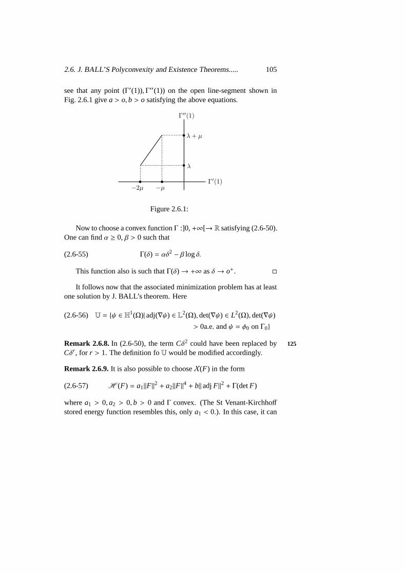
2.6. J. BALL’S Polyconvexity and Existence Theorems..... 105
see that any point (Γ′(1)), Γ′′(1)) on the open line-segment shown inFig. 2.6.1 givea > o, b > o satisfying the above equations.
Figure 2.6.1:
Now to choose a convex functionΓ :]0,+∞[→ R satisfying (2.6-50).One can findα ≥ 0, β > 0 such that
(2.6-55) Γ(δ) = αδ2 − β logδ.
This function also is such thatΓ(δ)→ +∞ asδ→ o+.
It follows now that the associated minimization problem hasat leastone solution by J. BALL’s theorem. Here
(2.6-56) U = ψ ∈ H1(Ω)|adj(∇ψ) ∈ L2(Ω), det(∇ψ) ∈ L2(Ω), det(∇ψ)
> 0a.e. andψ = φ0 onΓ0
Remark 2.6.8.In (2.6-50), the termCδ2 could have been replaced by125
Cδr , for r > 1. The definition foU would be modified accordingly.
Remark 2.6.9.It is also possible to chooseX(F) in the form
(2.6-57) H (F) = a1‖F‖2 + a2‖F‖4 + b‖adjF‖2 + Γ(detF)
wherea1 > 0, a2 > 0, b > 0 andΓ convex. (The St Venant-Kirchhoffstored energy function resembles this, onlya1 < 0.). In this case, it can
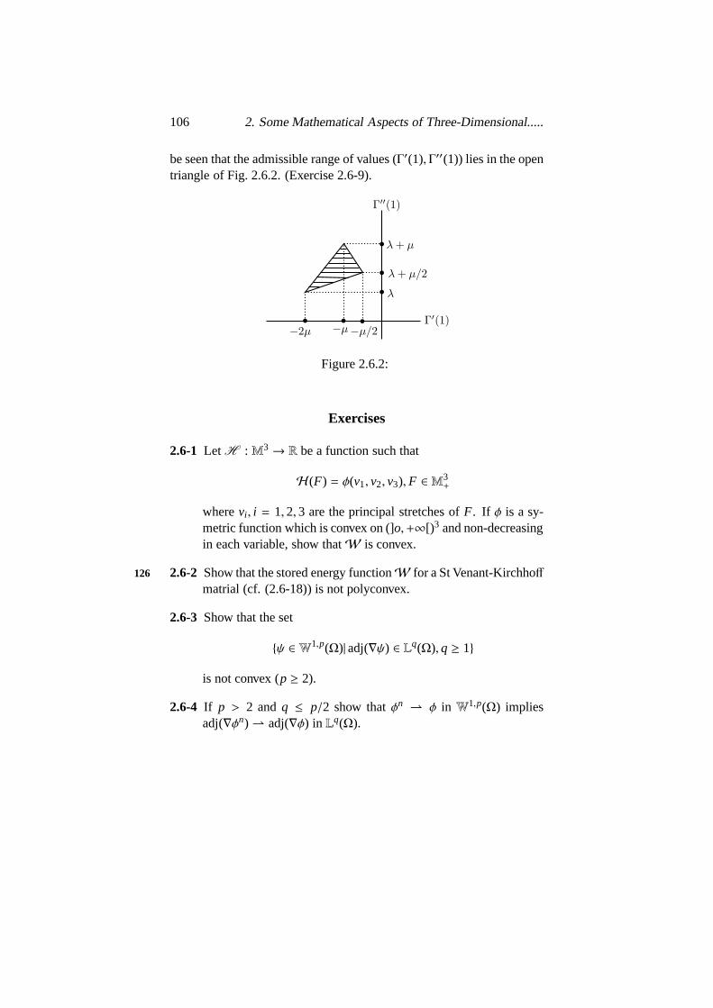
106 2. Some Mathematical Aspects of Three-Dimensional.....
be seen that the admissible range of values (Γ′(1), Γ′′(1)) lies in the opentriangle of Fig. 2.6.2. (Exercise 2.6-9).
Figure 2.6.2:
Exercises
2.6-1 Let H : M3→ R be a function such that
H(F) = φ(v1, v2, v3), F ∈ M3+
wherevi , i = 1, 2, 3 are the principal stretches ofF. If φ is a sy-metric function which is convex on (]o,+∞[)3 and non-decreasingin each variable, show thatW is convex.
2.6-2 Show that the stored energy functionW for a St Venant-Kirchhoff126
matrial (cf. (2.6-18)) is not polyconvex.
2.6-3 Show that the set
ψ ∈W1,p(Ω)|adj(∇ψ) ∈ Lq(Ω), q ≥ 1
is not convex (p ≥ 2).
2.6-4 If p > 2 andq ≤ p/2 show thatφn φ in W1,p(Ω) impliesadj(∇φn) adj(∇φ) in Lq(Ω).

2.6. J. BALL’S Polyconvexity and Existence Theorems..... 107
2.6-5 Show that there exists a constantd > 0 such that for allψ ∈W
1,p(Ω), ψ = ψ0 onΓ0,
∫
Ω
|ψ|pdx≤ d
∫
Ω
|∇ψ|pdx+
∫
Γo
|φo|da
p
.
2.6-6 If φn φ inW1,p(Ω) andφn = φo onΓo, show thatφ = φo onΓo.
2.6-7 Apply J. BALL’s theorem to the mixed diaplacement-pressureproblem.
2.6-8 . Let U be defined by
U = (φ,H) ∈ H1(Ω) × L2(Ω)|H = adj(∇φ), φ = φo onΓ0,
det(∇φ) = 1a.e
(incompressible case). AssumeU = D . (i) Show thatU is weaklyclosed in the product spaceH1(Ω) × L2(Ω). (ii) Consider
W(F) = a‖F‖2 + b‖adjF‖2, a > o, b > o,
I (ψ) =∫
Ω
W(∇ψ)dx− (∫
Ω
f .ψdx+∫
Γ1
g.ψda).
Show that the problem: Findφ ∈ U such that
U = φ ∈ H1(Ω); adj∇φ ∈ L2(Ω), φ = φo) on Γ0, det∇φ = 1a.e.I (φ) = inf
ψ∈UI (ψ)
has at least one solution. (iii) Ifφ is smooth, show that theLa- 127
grange multiplierarising out of equality constraint det(∇φ) = 1,is the pressure. (cf. Exercise 2.1-2).
2.6-9. Check the assertion made in Remark 2.6.9.

108 2. Some Mathematical Aspects of Three-Dimensional.....
Bibliography, Comments and some Open Problems128
No attempthas been made to give an exhaustive list of pertinentreferences.
The first chapter of these lecture notes gave a description ofelastic-ity in three demensions. For further refrences, one may alsoconsultGERMAIN [1972], GREEN and ZERNA [1968], GREEN and AD-KINS [1970], GURTIN [1981a, 1981 b], MARSDEN and HUGHES[1978,1983], STOKER [1968], TRUESDELL and NOLL [1956],VALID [1977], WANG and TRUESDELL [1973], ERINGEN [1962]and WASHING [1975].
The second chapter discussed some methods for proving the exis-tence of solution to the boundary value problem of non-linear elasticityand to the associated variational problem, in the case of hyperelasticmaterials.
For references about the linearized system of elasticity, see DU-VAUT and LIONS [1972], FICHERA [1972] and GURTIN [1972].
The key result in proving existence via theimplicit function theoremis theW2,p(Ω)-regularity of the linearized system of elasticity. The casep = 2 was proved by NECAS [1967] and the regularity for otherp wasproved by GEYMONAT [1965]. From this regularity result, (provedhowever only for the puredisplacement problem) the existence theoremwas independently proved by CIARLET and DESTUYNDER [1979b],MARSDEN and HUGHES [1978], VALENT [1979]. The basic idea,however, goes back to SPOPPELLI [1954] and VAN BUREN [1968].The extension of this result to more general constutive equations wasparticularly studied by VALENT [1979]. See also VALENT [1978a,1978b].
The necessity of theW2,p(Ω)-regularity of the linearized problem re-129
stricts the application of this method topure displacement problems.Itis also possible to treat thepure traction problem,which is more compli-cated owing to the compability conditions which the given forces mustsatisfy. For details see CHILLINGWORTH, MARSDEN and WAN[1982].
The increment method described in Section 2.4 is none other thanEuler’s method for approximating an appropriate differential equation
2.6. J. BALL’S Polyconvexity and Existence Theorems..... 109
in a Solbolev space. In other words, this method appears as aninfi-nite demensional version of the so calledcontinuation by differentiationapproach as described, for instance, in RHEINBOLDT [1974].
To the best of the author’s Knowledge, the convergence of incrementmethods for non-linear elasticity problems has been analysed so far onlyin some special cases, such as the one demensional model of a thin shal-low spherical shell, by ANSELONE and MOORE [1966] or some finitedimensional structural problems by RHEINBOLDT [1981]. Theresultspresented in these lecture can be found in BERNADOU, CIARLETandHU [1982].
For a decription of incremental methods in non-linear elasticity seeMASON [1980], ODEN [1972] and WASHIZU [1975].
The variation approach is based on the famous article of BALL[1977]. In addition to the notion ofpolycomvexityanother essentialcontribution of J. BALL is that one can pass to the weak limit in cer-tain non-convex sets as was seen in Section 2.6. This idea of compact-ness by compensation was also developed by MURAT [1978, 1979] andTARTAR [1979]. See also AUBERT and TAHRAOUI [1982].
Other important refrences are BALL [1981a,1981b, 1981c], BALL, 130
CURRIE and OLIVER [1981], BALL, KNOPS and MARSDEN [1978].See also EKELAND and TEMAN [1974] for the general problem ofminimizing functionals.
The notion of polyconvexity led to the definition of anOgden’s ma-terial (cf. OGDEN [1972]). ASt Venant-Kirchhoff material is not Og-den’s material and the existence of a solution to the corresponding mixeddisplacement-traction problem is open. In this connectionsee also AT-TEIA and DEDIEU [1981] and DACOROGNA [1982a, 1982b]. For yetanother approach, see ODEN [1979].
One of the drawbacks of J. BALL’s approach is the lack of regularityof the solution and so one does not know if the solution thus obtainedsatisfies theequilibrium equationeven in a weak sense. In this contex,see the results of LE TALLEC [1981] and LE TALLEC and ODEN[1981] for incompressible materials.
To conclude, we present a list of some of the open problems in non-linear elasticity. Some of them have been mentioned in the text before.

110 2. Some Mathematical Aspects of Three-Dimensional.....
1. LetC = ∇φT∇φ. If C − I is ’small’, in a sense to be made precise,can it be said thatφ is close to a rigid deformation? If some boundaryconditions are imposed, can it be shown thatφ is one-one?
In this context cf. KOHN [1982], ALEXANDER and ANTHAN[1982], ANTMAN [1979].
2. The standard implicit function theorem approach fails for mixed131
problems. Could “hard” implicit function theorem like thatof NASHand MOSER be used? In case of special domains like a thin plate, thesingularities are know explicity. Could this be used, and the implicitfunction theorem used only on the “regular” part of the solution?
3. Study of incremental methods taking into account the finite elementmethods.
4. An incremental method can beformally written down for the mixedproblem. If it can be shown to be convergent, this would provide anexistence theorem for the mixed problem.
5. The minimization procedure of J BALL does not imply that the so-lution is small if the forces are small. How can one “distinguish”the expected small solution in this case? (In the case of the puredisplacement problem, the solution via the implicit function theoremdoes not seem to be a local minimum of the energy in the “right”space).
6. A study plasticity has been taken up by TEMAN and STRANG-[1980a, 1980b]. They use the linear theory in the part correspondingto elasticity. Can one obtain better results by incorporating the non-linear theory, using J. BALL’s approach?
7. A study of ‘non local’ constotutive equations. Here the comstitutiveequation is of the form
T(x) =∫
B
ρk(x− y)T(∇φ(y))dy
whereρk is amollifier.

2.6. J. BALL’S Polyconvexity and Existence Theorems..... 111
8. One of thehardestopen problems of the study of theevolution prob- 132
lem which is a non-linear hyperbolic problem. The only availableresults are in the one-demensional case due to DIPERNA [1983].See also HUGHES, KATO and MARSDEN [1976].
9. Plate theory. A plate can be thought of as a domainΩ∈ = ω×]− ∈,+ ∈ [, whereω ⊂ R2 is a bounded open set and∈> o is a smallparameter. (cf. Fig.1)
Figure 1
By methods of asymptotic expansions, the solution (u∈, σ∈) can beformally expanded as
(u∈, σ∈) = (u0, σ0) + (u1, σ1) + · · ·
where (u0, σ0) satisfies a well-known two-dimensional plate model.In the linearized theory CIARLET and DESTUYNDER [1980a],CIARLET and KESAVAN [1980], DESTUYNDER [1980] have stu-died the problems extensively. One can compare the three dimen-sional and two dimensional problems and show that (for example)
‖u∈3d − u∈2d‖1,Ω∈‖u∈3d‖1,Ω∈
→ o as ∈→ 0.
The problem is tonumericallyverify this. Computing by the finiteelement method, one getsu∈3d,h andu∈2d,h approximatingu∈3d andu∈2drespectively. Since∈ is small, unlessh is of the same order, the linear 133
systems become very ill-conditioned. But ifh is of the same orderof ǫ, the solutionuǫ3d,h is not very accurate. Thus to find a bettermethod of approximating these solutions and verify the convergencedescribed above.

112 2. Some Mathematical Aspects of Three-Dimensional.....
10. In the nonlinear case CIARLET [1980] (see also CIARLET and-DESTUYNDER [1979], CIARLET and RABIER [1980]) has shownthat with certain boundary conditions the three dimensional platemodel for a St Venant -Kirchhoffmaterial is approximated (formally)by the well-known two-dimensional von Karman model. While thelatter has a satisfactory existence theorey, the former hasnone. If atleast forǫ small enough it can be shown that the three dimensionalproblem has a solution converging to a given solution of the dimen-sional problem, an existance theorem for such special domains canbe obtained.
Bibliography
134[1] ADAMS, R.A. (1975): Sobolev Spaces, academic Press, New
York.
[2] AGMON, S., DOUGLIS,A. and NIRENBERG,L.(1959): Esti-mates near the boundary for solutions of elliptic partial defferentialequations satisfying general boundary conditionsI . Comm. PureAppl. Math., 12,pp.623-727.
[3] AGMON, S.,DOUGLIS,A. and NIRENBERG,L.(1964): Esti-mates near the boundary for solutions of elliptic partial defferentialequations satisfying general boundary conditionsII , Comm. PureAppl. Math., 17,pp.35-92.
[4] ALEXANDER, J.C. and ANTMAN,S.S. (1982): The ambiguoustwist of Love, Quart. Appl. Maths., pp.83-92.
[5] ANSELONE,P.M. and MOORE (1966): An extension of the New-ton Kantorovic method for solving nonlinear equation with an ap-plication to elasticity, J.Math.Anal. Appl., 13.pp. 476-501.
[6] ANTAM, S.S.(1979): The eversion of thick spherical shells, Arch.Rational Mech . Anal., 70,pp.113-123.
[7] ATTEIA,M. and DEDIEU,J.P.(1981): Minimization of energy innon linear elasticity, in Nonlinear Problems of analysis inGeom-etry and Mechanics, [M.ATTEIA, D. BANCEL, I. GUMOWSKI,Editors], pp.73-79, Pitman, Boston
113

114 BIBLIOGRAPHY
[8] AUBERT,G.and TAHRAOUI,R.(1982): Sur la faible fermeture decertain ensembles de contraintes en elasticite non-lineaire plane,Arch. Rational Mech. Anal, to appear.
[9] BALL,J.M. (1977): Convexity conditions and existance theorems135
in nonlinear elasticity, arch. Rational. Mech. Anal., 63,pp.337-403.
[10] BALL,J.M.(1981a): Discontinuous equilibrium solutions andcavitions in non-linear elasticity, Phil. Trans. Rayal Soc. London,to appear.
[11] BALL,J.M. (1981b): Remarques surℓ′ existance et la regularitedes solutions d’elastostatique non-lineare, in Recent Contributinsto Nonlinear Partial Differential Equations, pp.50-62, Res. Notesin Math., 50, Pitman, Boston.
[12] BALL,J.M. (1981c): Global invertibility of ’Sobolev functions andthe interpenetration of matter,Proc. Royal Soc. Edinburgh, 88A,pp.315-328.
[13] BALL,J.M., CURRIE,J.C. and OLVER,P.J.(1981): Null La-grangians, weak continuit and variational problems of arbitrary or-der, J.Functional analysis, 41, pp.135-174.
[14] BALL,J.M., KNOPS,R.J. and MARSDEN,J.E. (1978): Two ex-amples in non-linear elasticity, in Proceedings, conference onnonlinear Analysis, Besancon, 1977, pp.41-49, Springs-Verlag,Berlin.
[15] BERNADOU,M., CIARLET, P.G. and HU,J. (1982): Sur la con-vergence des methodes incrementales en elasticite non-linearetridimensionnelle. C.R.Acad, Sc. Paris, Serie I, 295. 639-642.
[16] CHILLINGWORTH,D.R.J.,MARSDEN, J.E.and WAN, Y.H.(1982): Symmetry and bifurcation in three dimensional elasticity.PartI ., Arch. Rational Mech, Anal., 80, pp.295-331.
[17] CIARLET,P.G. (1980): A justification of the von Karman equa-tions, Arch. Rational Mech.Anal., 73, pp.349-389.
BIBLIOGRAPHY 115
[18] CIARLET, P.G. and DESTUYNDER,P.(1979a): A justification of 136
the two-dimensional linear plate model, J.Mecanique, 18, pp.315-344.
[19] CIARLET,P.G. and DESTUYNDER,P.(1979b): A justification ofa nonlinear model in plate theory, Compute. Methods Appl. Mech.Engrg., 17/18, pp.227-258.
[20] CIARLET,P.G. and GEYMONAT,G.(1982): Sur les lois de com-portment en elasticite non-lineaire compressible, C.R. Acad. Sci.Paris, Serie A., 295,pp.423-426.
[21] CIARLET,P.G. and KESAVAN,S.(1980): Tow dimensional ap-proximations of three-dimensional eigenvalues in plate theory,Compute. Methods Appl. Mech. Engrg., 26, pp.149-172.
[22] CIARLET, P.G. and RABIER, P. (1980): Les Equations devon Karman, Lecture notes in Mathematics, Vol. 826, Springer-Verlag,Berlin.
[23] DACOROGNA,B.(1980a): Weak Continuity and Weak LowerSemicontinuity of Non-Linear Functionals. Lecture Notes inMathematics, Vol.922, Springer-Verlag, Berlin.
[24] DACOROGNA,B. (1982b): Quasiconvexity and relaxationof non-convex problems in the calculus of variations, j. Functional Anal-ysis 46, pp.102-118.
[25] DESTUYNDER,P. (1980): Sur une Justification dea Modelesde plaques et de Coques par les Methodes Asymptotiques, The-sis,univesite Pierre et Marie Curie, Paris.
[26] DESTUYNDER,P. and GALBE,G.(1978): Analyticite de la so-lution d′ un probleme hyperelastique nonlineare, C.R. Acad. Sci.Paris, Serie A, pp.365-368.
[27] DIPERNA, R.J.(1983): To appear 137
[28] DUVAUT,G. and LIONS,J.L.(1972): Les Inequations enMecanique et en Physique, Dunod, Paris.

116 BIBLIOGRAPHY
[29] EKELAND, I, and TEMAM,R.(1974): Analyse Convexe et Prob-lems Variationnels, Dunod, PAris. (English Translation: ConvexAnalysis and Variational Problems, North Holland, Amsterdam,1975).
[30] ERINGEN,A.C. (1962): Nonlinear Theoey of Continuous Media,McGraw-Hill, New York.
[31] FICHERA,G.(1972): Existence theorems in elasticity,Handbuchder Physik, VIa/2, Springer, Berlin.
[32] GERMAIN,P.(1972): Mecanique des Milieux Continuous,Tome1 Massan, Paris.
[33] GEYMONAT,G.(1965): Sui problems ai limiti peri sistemi lineariellitici, Ann. Mat. Pura. Appl., 69, pp.207-284.
[34] GREEN,A.E. and ADKINS, J.E. (1970): Large Elastic Deforma-tions, Second Edition, Clarendon Press, Oxford.
[35] GREEN,A.E. and ZERNA, W.(1968): Theoretical Elasticity, uni-versity Press, Oxford.
[36] GURTIN, m.E. (1972): The linear theory of elasticity, in Hand-buch der Physik, pp.1-295, Vol. VIa, Springer-Verlag, Berlin.
[37] GURTIN,M.E.(1981a): Topics in Finite Elasticity, CBMS-NSFRegional Conference Series in Applied Mathematics, SIAM,Philadephia.
[38] GURTIN,M.E. (1981b): Introduction to Continuous Mechanics,Academic Press, New York.
[39] HUGHES, T.J.R., KATO, T, and MARSDEN,J.E.(1976): Well-138
posed quasi linear second -order hyperbolic system with applica-tions to non-linear elastodynamics and general relativity, Arch. Ra-tional Mech. Anal., 63, pp. 273-304.
BIBLIOGRAPHY 117
[40] JOHN,F.(1972): Uniqueness of non-linear elastic equilibrium forprescrbed boundary displacements and sufficiently small strains,Comm. Pure Appl. Math., XXV, pp.617-634.
[41] KOHN, R.V. (1982): New integral estimates for deformations interms of their nonlinear, Arch. Rational Mech, Anal., 78, pp. 131-172.
[42] LE DRET,H. (1982): Thesis, Universite Pierre et MArie Curie,Paris.
[43] LE TALLEC,P. (1981): Existence and approximation results fornon-linear mixed problems: applications to incompressible finiteelasticity, (to appear).
[44] LE TALLEC, P. and ODEN,J.T. (1981): Existence and characteri-zation of hydrostatic pressure in finite deformations of incompress-ible elastic bodies, J. Elasticity, 11, pp.341-358.
[45] MARSDEN,J.E. and HUGHES, T.J.R. (1978): Topics in the math-ematical foundations of elasticity, in Nonlinear Analysisand Me-chanics: Heriot-Watt Symposim, Vol.2, pp.30-285, Pitman,Lon-don.
[46] MARSDEN,J.E. and HUGHES, T.J.R. (1983): MathematicalFoundations of Elasticity, Prentice-Hall, Englewood Cliffs.
[47] MASON,J. (1980): Variational, Incremental and EnergyMethodsin Solid Mechanics and Shell Theory, Elsevier, Amsterdam.
[48] MEISTERS,G.H. and OLECH, C. (1963): Locally one-to -onemapping and a classical theorem on Schlicht functions, DukeMath. J., 30, pp.63-80.
[49] MURAT, F. (1978): Compacite par compesation,Annali Scu. 139
Norm. Sup. Pisa. IV, 5, pp. 489-507.
[50] MURAT,F.(1979): Compacite par compensation II. ProceedingsInternational Conference on recent Methods in-Linear Analysis,Rome, 1978, Pitagora, Bologna,
118 BIBLIOGRAPHY
[51] NECAS,J.(1967): Les Methodes Directes en Theorie des Equa-tions Elliptiques, Masson, Paris.
[52] NITSCHE,J.A. (1981): On Korn’s Second inequality, RAIRO,Analyse Numerique, Vol.15, No.3, pp. 237-248.
[53] ODEN,J.T. (1972): Finite Elements of Nonliner Continua,McGraw-Hill New York.
[54] ODEN,J.T.(1979): Existance theorems for a class of problems innon-linear elasticity, J. Math.Anal. Appl., 69, pp.51-83.
[55] OGDEN, R.W. (1972): Large deformation isotrophic elasticity:On the correlation of theory and experiment for compressible rub-berlike solids, proc. Roy. Soc. London, A 328, pp.567-583.
[56] RHEINBOLDT,W.C. (1974): Methods for Solving Systems ofNonlinear Equations, CBMS Series, No.14, SIAM, Philadephia.
[57] RHEINBOLDT,W.C. (1981): Numerical analysis of continuationmethods for nonlinear structure problems, Computers and struc-tures, 13, pp.103-113.
[58] STOKER,J.J.(1968): Nonlinear Elasticity, Gordon andBreach,New York.
[59] STOPPELLI,F.(1954): Un teorema di esistenza e di unicita rel-ativo alle equazioni dell’ elastostatica isoterma per deformazionifinite, Ricerche di Matematica, 3, pp.247-267.
[60] TARTAR, L. (1979): Compensated compactness and partial dif-140
ferential equation, in Nonlinear Analysis Mechanics: Heriot-WattSymposim, Vol. IV,(R.J.knops, Ed.) Pitman, pp.136-212.
[61] TEMAM,R. and STRANG,G. (1980a): Duality and relaxation inplasticity, J. de Mecanique, 19, pp.1-35.
[62] TEMAM, R. and STRANG, G.(1980b): Functions of bounded de-formation Arch. Rational Mech.Anal., 75, pp.7-21.

BIBLIOGRAPHY 119
[63] TRUESDELL,C. and NOLL,W. (1965): The Non-linear field the-ories of Mechanics. Handbuch der Physik, Vol.III/3, Springer,Berlin.
[64] VALENT,T. (1978a): Sulla Defferenziabilita di un operatore legatoa una classe di sistemi differenziali quasi-lineari, Rend. Sem. Mat.Univ. Padova, 57,pp.311-322.
[65] VALENT,T. (1978b): Osservazioni sulla linearizzazione di un op-eratore differenziale, Rend. Acc. Naz. Lincei, 65,pp.27-37.
[66] VALENT, T. (1979): Teoremi di esistenza e unicita in elastostaticafinite, Rend. Sem. Mat. univ. Padova, 60, pp.165-181.
[67] VALID,R. (1977): La Mecanique des Milieux Continus et leColoul des Structures. Eyrolles, Paris. (English translation: Me-chanics of Continuous Media and Analysis of Stuctures North-Holland, Amsterdam, 1981).
[68] VAN BUREN, M. (1968): On the Existence and Uniqueness ofSolutions to Boundary Value Problems in Finite Elasticity,Thesis,Carnegie-Mellon University.
[69] WANG, C,-C. and TRUESDELL,C.(1973): Introduction to Ratio-nal Elasticity, Noordhoff, Groningen.
[70] WASHIZU, K.(1975): Variational Methods in Elasticityand Plas-ticity, Second Edition, Pergamon, Oxford.
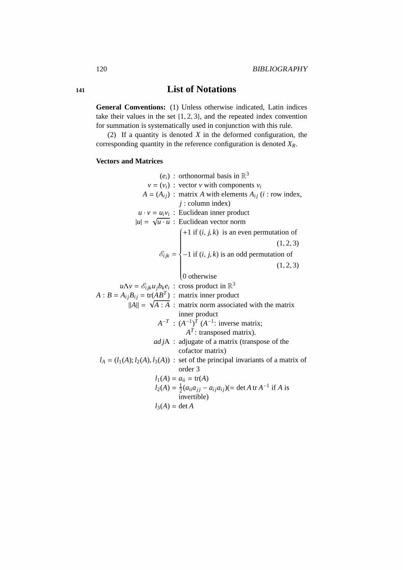
120 BIBLIOGRAPHY
List of Notations141
General Conventions: (1) Unless otherwise indicated, Latin indicestake their values in the set1, 2, 3, and the repeated index conventionfor summation is systematically used in conjunction with this rule.
(2) If a quantity is denotedX in the deformed configuration, thecorresponding quantity in the reference configuration is denotedXR.
Vectors and Matrices
(ei) : orthonormal basis inR3
v = (vi) : vectorv with componentsvi
A = (Ai j ) : matrix A with elementsAi j (i : row index,j : column index)
u · v = uivi : Euclidean inner product|u| =
√u · u : Euclidean vector norm
Ei jk =
+1 if (i, j, k) is an even permutation of
(1, 2, 3)
−1 if (i, j, k) is an odd permutation of
(1, 2, 3)
0 otherwiseuΛv = Ei jku jbkei : cross product inR3
A : B = Ai j Bi j = tr(ABT) : matrix inner product||A|| =
√A : A : matrix norm associated with the matrix
inner productA−T : (A−1)T (A−1: inverse matrix;
AT : transposed matrix).ad jA : adjugate of a matrix (transpose of the
cofactor matrix)lA = (l1(A); l2(A), l3(A)) : set of the principal invariants of a matrix of
order 3l1(A) = aii = tr(A)l2(A) = 1
2(aii a j j − ai j ai j )(= detA tr A−1 if A isinvertible)
l3(A) = detA

BIBLIOGRAPHY 121
M3 : set of all matrices of order 3M
3+ = F ∈ M3|detF > 0O
3 = F ∈ M3|FT F = FFT = I O
3+ = O
3 ∩ M3+ = F ∈ O3|detF = 1
S3 = F ∈ M3|F = FTS
3> = F ∈ S3|F is positive definite
F = RU = VR : polar factorization of an invertiblematrix (R ∈ O3; U,V ∈ S3
>)C1/2 : square root of a matrixC ∈ S3
>
142
Functions and Function Spaces
Id : identity mappingv′(a) : Frechet derivative of the mappingv at the
point a
∂αv =∂|α|v
∂xα11 . . . ∂xαn
n, |α| = α1 + · · · + αn
(multi-index notation for partialderivatives)
∂W
∂F(F) =
(
∂W
∂Fi j(F)
)
∈ M3 (for a mapping
W : M3→ R)X → Y : the canonical injection fromX into Y is
continuous
Xc→Y : the canonical injection fromX into Y is
compact : weak convergence
C0(X,Y) : set of all continuous mappings fromXinto Y
Cm(X; Y) : space of allm times continuouslydifferentiable mappings fromX intoY(1 ≤ m≤ ∞)
Cm(X) = Cm(X;R), 0 ≤ m≤ ∞.Wm,p(Ω) = v ∈ Lp(Ω); ∂αv ∈ Lp(Ω) for all |α| ≤ m
(W0,p(Ω) = Lp(Ω))

122 BIBLIOGRAPHY
Hm(Ω) =Wm,2(Ω)L
p(Ω),Wm,p(Ω),Hm(Ω) : corresponding spaces of vector-valued, ormatrix-valued, functions
|v|0,p,Ω : norm of the spaceLp(Ω), 1≤ p ≤ ∞.||v||m,p,Ω =
∫
Ω
∑
|α|≤m|∂αv|pdx1/p: norm of the space
Wm,p(Ω), 1 ≤ p ≤ ∞||v||m,∞,Ω = max
|α|≤m|∂αv|0,∞,Ω: norm of the space
Wm,∞(Ω)|v|m,p,Ω =
∫
Ω
∑
|α|=m|∂αv|pdx1/p, 1≤ p ≤ ∞
|v|m,∞,Ω = max|α|=m|∂αv|0,∞,Ω
D(Ω) = v ∈ C∞(Ω); suppv is a compact subset ofΩ
Wm,p0 (Ω) : closure ofD(Ω) in Wm,p(Ω)Hm
0 (Ω) =Wm,20 (Ω)
143
Miscellaneous
[a,+∞] = [a,+∞[∪+∞, a ∈ R
f (x) = 0(x) : limx→0x,0
| f (x)|||x|| = 0
c U : convex hull ofU (smallest convex setcontainingU)
Notations in the Deformed Configuration144
B = φ(BR) : deformed configurationX = φ(XR) : generic point ofB
∂B : boundary ofB∂B = ∂B0 ∪ ∂B1 : dA-measurable partition of∂B
n : unit outer normal along∂BdX : volume element inBdA : surface element on∂B

BIBLIOGRAPHY 123
GRADΘ =
(
∂Θi
∂X j
)
∈ M3 (for a mappingΘ : B → R3)
DIV T =∂Ti j
∂X jei ∈ R3 : divergence of a tensor fieldT : B → M3
∂(X) ∈ R : density per unit mass atX ∈ B
b(X) ∈ R3 : body force density per unit mass atX ∈ B
t1(X) ∈ R3 : applied surface force density per unit areaof ∂B at X ∈ ∂B
t(X, n),X ∈ B, |n| = 1 : Cauchy stress vector inBT(X) : Cauchy stress tensor atX ∈ B
T,T : response function forT = T(F) = T(B),with F ∈ M3
+, B = FFT .
Notations in the Reference Configuration 145
BR, orΩ : reference configurationXR, or x : generic point ofBR
∂BR, or Γ : boundary ofBR
∂BR = ∂B0R∪ ∂B1R, or Γ = Γ0 ∪ Γ1 : dAR-measurable partition of∂BR
nR, or ν : unit outer normal along∂BR
dXR, or dx : volume element inBR
dAR, or da : surface element on∂BR
φ, ψ : BR→ R3 : deformation ofBR (smoothmaps with det· > 0)
u, v : BR→ R3 : displacement(φ = Id+u, ψ = Id+v)
∂i =∂
∂XRi
DIVRTR =∂TRi j
∂XRjei ∈ R3 : divergence of a tensor field
TR : BR→ M3
∇φ =(
∂φi∂XRj
)
∈ M3+ : deformation gradient
∇u =
(
∂ui∂XRj
)
∈ M3 : displacement gradient
C = ∇Tφ∇φ ∈ S3
> : right Cauchy-Green straintensor
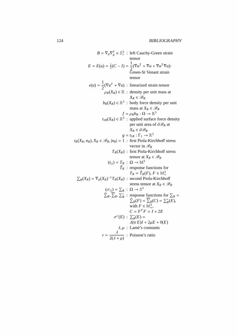
124 BIBLIOGRAPHY
B = ∇φ∇Tφ ∈ S3
> : left Cauchy-Green straintensor
E = E(u) = 12(C − I ) =
12
(∇uT + ∇u+ ∇uT∇u):
Green-St Venant straintensor
ǫ(u) =12
(∇uT + ∇u) : linearized strain tensor
ρR(XR) ∈ R : density per unit mass atXR ∈ BR
bR(XR) ∈ R3 : body force density per unitmass atXR ∈ BR
f = ρRbR : Ω→ R3
t1R(XR) ∈ R3 : applied surface force densityper unit area of∂BR atXR ∈ ∂BR
g = t1R : Γ1→ R3
tR(XR, nR),XR ∈ BR, |nR| = 1 : first Piola-Kirchhoff stressvector inBR
TR(XR) : first Piola-Kirchhoff stresstensor atXR ∈ BR
(ti j ) = TR : Ω→ M3
TR : response functions forTR = TR(F), F ∈ M3
+∑
R(XR) = ∇φ(XR)−1TR(XR) : second Piola-Kirchhoffstress tensor atXR ∈ BR
(σi j ) =∑
R : Ω→ S3
ˆ∑R,
∑
R,∑∗
R : response functions for∑
R =ˆ∑
R(F) =∑
R(C) =∑∗
R(E),with F ∈ M3
+,C = FTF = I + 2E
σ∗(E) :∑∗
R(E) =λ(tr E)I + 2µE + 0(E)
λ, µ : Lame’s constants
ν =λ
2(λ + µ): Poisson’s ratio
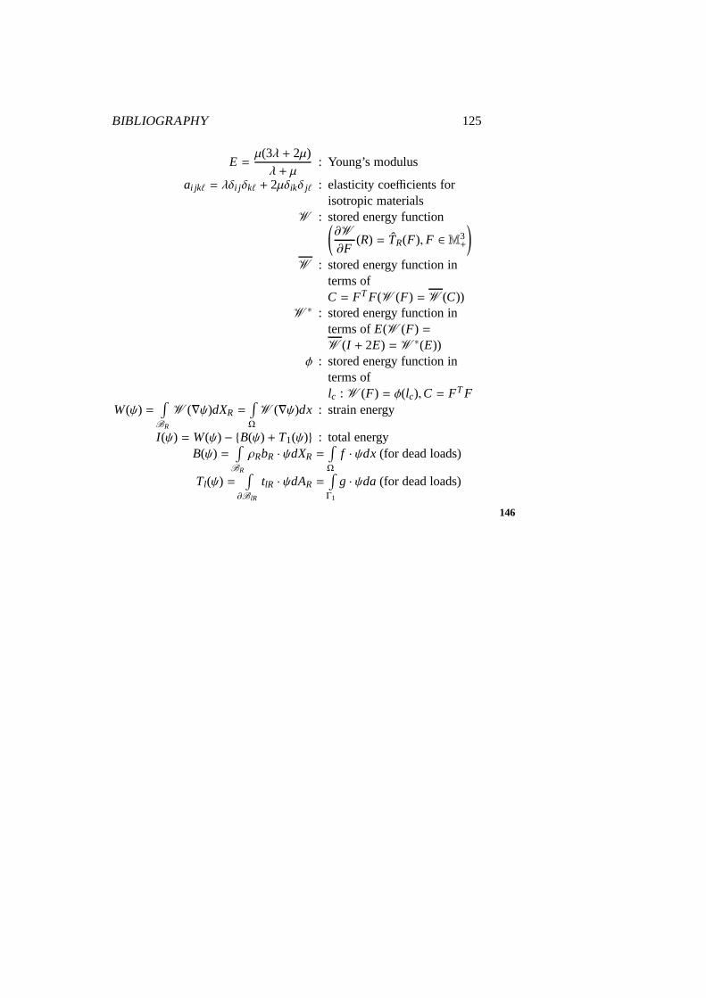
BIBLIOGRAPHY 125
E =µ(3λ + 2µ)λ + µ
: Young’s modulus
ai jkℓ = λδi jδkℓ + 2µδikδ jℓ : elasticity coefficients forisotropic materials
W : stored energy function(
∂W
∂F(R) = TR(F), F ∈ M3
+
)
W : stored energy function interms ofC = FTF(W (F) = W (C))
W ∗ : stored energy function interms ofE(W (F) =W (I + 2E) = W ∗(E))
φ : stored energy function interms oflc : W (F) = φ(lc),C = FTF
W(ψ) =∫
BR
W (∇ψ)dXR =∫
Ω
W (∇ψ)dx : strain energy
I (ψ) =W(ψ) − B(ψ) + T1(ψ) : total energyB(ψ) =
∫
BR
ρRbR · ψdXR =∫
Ω
f · ψdx (for dead loads)
Tl(ψ) =∫
∂BlR
tlR · ψdAR =∫
Γ1
g · ψda (for dead loads)
146
Index
Aapplied surface force, 9applied surface force, 18axiom of material frame indifference, 21axiom of static equilibrium, 9, 19
Bbody force, 9body force, 17boundary condition of traction, 54boundary condition of pressure, 55boundary condition of place, 54
CCauchy stress vector, 13Cauchy stress tensor, 12, 29Cauchy stress vector, 9, 21Cauchy’s Theorem, 10Cauchy-Green strain tensors, 5conservative applied surface force, 18conservative body force, 18constitutive equation, 20
DDa Silva’s Theorem, 19dead load, 17deformation, 2, 32deformation gradient, 2deformed configuration, 2displacement, 2displacement gradient, 3divergence of a tensor, 3
Eelastic material, 20elasticity coefficient, 36
energy, 39equilibrium equations, 16, 37Euler equation, 39Euler’s method, 81Eulerian variable, 14
Fforce: applied surface, 9, 18
body, 9, 17surface, 9system of, 9
GGreen-St Venant strain tensor, 7Green-St Venant strain tensor, 30
Hhomogeneous material, 20homogeneous deformation, 32hyperelastic material, 38
Iincompressible material, 34incompressible material, 107incompressible material, 62incremental method, 80infinitesimal rigid displacement, 19isotropic response function, 26isotropic material, 23isotropic response function, 23isotropic stored energy function, 40, 44
KKorn’s inequality, 64
LLagrangian variable, 14
126
INDEX 127
LAM E’s constants, 31, 50, 103linearized strain tensor, 63linearized system of elasticity, 62, 78, 89
Mmaterial
elastic, 20homogeneous, 20hyperelastic, 38incompressible, 34, 62, 107isotropic, 23MOONEY-RIVLIN, 93non-homogeneous, 20OGDEN’s, 92, 104St Venant-Kirchhoff, 35, 49, 68, 84,
89, 93, 106material frame indifference, 21, 26, 29,
40, 43, 89mixed displacement-pressure problem,
55, 107mixed displacement-tranction problem,
54, 78, 84, 103MOONEY-RIVLIN material, 93
Nnatural state, 31non-homogeneous material, 20
OOGDEN’s material, 92, 104
PPiola identity, 7, 98Piola transform, 4, 14Piola-Kirchhoff stress tensors, 14, 15, 29,
43, 45Piola-Kirchhoff stress vector, 16Poisson’s ratio, 35polar factorisation of a matrix, 20polyconvix stored energy function, 91,
92, 100pressure, 17, 19, 33, 107principal invariants of a matrix, 25principal stretch, 92, 106principle of virtual work, 14, 17, 19pure displacement problem, 54, 68, 80
pure pressure problem, 55pure traction problem, 54
Rreference configuration, 1response function, 20rigid deformation, 6Rivlin-Ericksen Theorem, 26
SSt Venant-Kirchhoff material, 35, 49, 68,
84, 89, 93, 106stored energy function, 39strain
- energy, 39CAUCHY-GREEN-tensors, 5Green-St Venant-tensor, 7, 30linearized -tensor, 63
stressCAUCHY - tensor, 12, 29CAUCHY - vector, 9, 13, 21PIOLA-KIRCHHOFF - tensors, 14,
15, 29, 43, 45PIOLA-KIRCHHOFF - vector, 16
surface force, 9system of forces, 9
Ttotal energy, 39
Uunilateral boundary condition, 55
YYOUNG’s modulus, 35