arX

iv:1

609.

0952

3v5

[he

p-th

] 1

3 M

ar 2

019

Minimal lectures on two-dimensional

conformal field theory

Sylvain Ribault

CEA Saclay, Institut de Physique Theorique

sylvain.ribault@ipht.fr

March 14, 2019

Abstract

We provide a brief but self-contained review of two-dimensional conformal fieldtheory, from the basic principles to some of the simplest models. From the represen-tations of the Virasoro algebra on the one hand, and the state-field correspondenceon the other hand, we deduce Ward identities and Belavin–Polyakov–Zamolodchikovequations for correlation functions. We then explain the principles of the conformalbootstrap method, and introduce conformal blocks. This allows us to define andsolve minimal models and Liouville theory. In particular, we study their three- andfour-point functions, and discuss their existence and uniqueness. In appendices, weintroduce the free boson theory (with an arbitrary central charge), and the modularbootstrap in minimal models.

Based on lectures given at the school on “Quantum integrable systems, conformal fieldtheories and stochastic processes” (Cargese, September 2016), and at the “Young Re-searchers Integrability School” (Vienna, February 2019).

An earlier version of this text was published in SciPost Physics Lecture Notes: arXiv’sfourth version arXiv:1609.09523v4.

1

Contents

0 Introduction 2

1 The Virasoro algebra and its representations 3

1.1 Algebra . . . . . . . . . . . . . . . . . . . . . . . . . . . . . . . . . . . . . 31.2 Representations . . . . . . . . . . . . . . . . . . . . . . . . . . . . . . . . . 41.3 Null vectors and degenerate representations . . . . . . . . . . . . . . . . . 5

2 Fields and correlation functions 6

2.1 Fields . . . . . . . . . . . . . . . . . . . . . . . . . . . . . . . . . . . . . . 72.2 Correlation functions and Ward identities . . . . . . . . . . . . . . . . . . . 82.3 Belavin–Polyakov–Zamolodchikov equations . . . . . . . . . . . . . . . . . 10

3 Conformal bootstrap 10

3.1 Single-valuedness . . . . . . . . . . . . . . . . . . . . . . . . . . . . . . . . 113.2 Operator product expansion and crossing symmetry . . . . . . . . . . . . . 113.3 Degenerate fields and the fusion product . . . . . . . . . . . . . . . . . . . 14

4 Minimal models 15

4.1 Diagonal minimal models . . . . . . . . . . . . . . . . . . . . . . . . . . . . 164.2 D-series minimal models . . . . . . . . . . . . . . . . . . . . . . . . . . . . 17

5 Liouville theory 18

5.1 Definition . . . . . . . . . . . . . . . . . . . . . . . . . . . . . . . . . . . . 185.2 Three-point structure constants . . . . . . . . . . . . . . . . . . . . . . . . 195.3 Crossing symmetry . . . . . . . . . . . . . . . . . . . . . . . . . . . . . . . 22

A Side subjects 23

A.1 Free boson . . . . . . . . . . . . . . . . . . . . . . . . . . . . . . . . . . . . 23A.2 Modular bootstrap . . . . . . . . . . . . . . . . . . . . . . . . . . . . . . . 26

B Solutions of Exercises 28

List of Exercises 36

References 36

0 Introduction

Two-dimensional CFTs belong to the rare cases of quantum field theories that can be ex-actly solved, thanks to their infinite-dimensional symmetry algebras. They are interestingfor their applications to statistical physics, they are the technical basis of string theory inthe worldsheet approach, and they can guide the exploration of higher-dimensional CFTs.

We will introduce the main ideas of two-dimensional CFT in the conformal bootstrapapproach, and focus on the simplest nontrivial models that have been solved: minimalmodels and Liouville theory. Rather than following the history of the subject, we tryto derive the results in the simplest possible way. While not claiming mathematicalrigour, we explicitly state the axioms that underlie our derivations. This is supposed tofacilitate generalizations, for example to CFTs based on larger symmetry algebras, or tonon-diagonal CFTs [1].

2

Our first axioms will specify how the Virasoro symmetry algebra acts on fields, and theexistence and properties of the operator product expansion. Next, we introduce additionalaxioms that single out either minimal models, or Liouville theory. We will then checkthat these theories actually exist, by studying their four-point functions. It is the successof such checks, more than a priori considerations, that justifies our choice of axioms.

Our main tool for solving CFTs is crossing symmetry of the sphere four-point function.We will however introduce two other tools as side subjects:

• The free boson (Appendix A.1) is not needed in our approach, because we do notbuild CFTs as perturbed free theories, as is done in the Lagrangian approach. How-ever, it is a good preparation to the study of CFTs based on larger symmetryalgebras, in particular WZW models.

• The modular bootstrap (Appendix A.2) focuses on torus partition functions: lessinteresting than sphere four-point functions, but also much simpler, so they can betractable even in complicated models.

This text aims to be self-contained, except at the very end when we will refer to [2] forthe properties of generic conformal blocks. For a more detailed text in the same spirit,see the review article [3]. For a wider and more advanced review, and a guide to therecent literature, see Teschner’s text [4]. The Bible of rational conformal field theory isof course the epic textbook [5]. And Cardy’s lecture notes [6] provide an introduction tothe statistical physics applications of conformal field theory.

Exercise 0.1 (Update Wikipedia)How would you rate Wikipedia’s coverage of two-dimensional CFT? For a list of somerelevant articles, see this page. Correct and update these articles when needed. Are thereother relevant articles? Which articles should be created?

Acknowledgements

I am grateful to the organizers of the Cargese school, for challenging me to explain Liou-ville theory in about four hours. I am grateful to the organizers of the Vienna school, forthe opportunity to fit these lectures into a school on various aspects of two-dimensionalCFT.

I wish to thank Bertrand Eynard, Riccardo Guida, Yifei He, and Andre Voros for help-ful suggestions and comments. I am grateful to the participants of the Cargese and Viennaschools, for their stimulating participation in the lectures. I wish to thank the SciPosteditor and reviewers for their feedback and suggestions, which led to many improvements,both perturbative and non-perturbative.

1 The Virasoro algebra and its representations

1.1 Algebra

By definition, conformal transformations are transformations that preserve angles. Intwo dimensions with a complex coordinate z, any holomorphic transformation preservesangles. Infinitesimal conformal transformations are holomorphic functions close to theidentity function,

z 7→ z + ǫzn+1 (n ∈ Z , ǫ ≪ 1) . (1.1)

3

These transformations act on functions of z via the differential operators

ℓn = −zn+1 ∂

∂z, (1.2)

and these operators generate the Witt algebra, with commutation relations

[ℓn, ℓm] = (n−m)ℓm+n . (1.3)

The generators (ℓ−1, ℓ0, ℓ1) generate a subalgebra called the algebra of infinitesimalglobal conformal transformations and isomorphic to sℓ2. The corresponding Lie group isthe group of global conformal transformations of the Riemann sphere C ∪ {∞},

z 7→ az + b

cz + d, (a, b, c, d ∈ C, ad− bc 6= 0) . (1.4)

Exercise 1.1 (Global conformal group of the sphere)Show that the global conformal group of the sphere is PSL2(C), and includes translations,rotations, and dilations.

In a quantum theory, symmetry transformations act projectively on states. Projectiverepresentations of an algebra are equivalent to representations of a centrally extendedalgebra. This is why we always look for central extensions of symmetry algebras.

Definition 1.2 (Virasoro algebra)The central extension of the Witt algebra is called the Virasoro algebra. It has thegenerators (Ln)n∈Z and 1, and the commutation relations

[1, Ln] = 0 , [Ln, Lm] = (n−m)Ln+m +c

12(n− 1)n(n + 1)δn+m,01 , (1.5)

where the number c is called the central charge. (The notation c1 stands for a centralgenerator that always has the same eigenvalue c within a given conformal field theory.)

Exercise 1.3 (Uniqueness of the Virasoro algebra)Show that the Virasoro algebra is the unique central extension of the Witt algebra.

1.2 Representations

The spectrum, i.e. the space of states, must be a representation of the Virasoro algebra.Let us now make assumptions on what type of representation it can be.

Axiom 1.4 (Representations that can appear in the spectrum)The spectrum is a direct sum of irreducible representations. In the spectrum, L0 isdiagonalizable, and the real part of its eigenvalues is bounded from below.

Why this special role for L0? Because we want to interpret it as the energy operator. Wehowever do not assume that L0 eigenvalues are real or that the spectrum is a Hilbert space:this would restrict the central charge to be real. The L0 eigenvalue of an L0 eigenvectoris called its conformal dimension. The action of Ln shifts conformal dimensions by −n:

L0|v〉 = ∆|v〉 ⇒ L0Ln|v〉 = LnL0|v〉+ [L0, Ln]|v〉 = (∆− n)Ln|v〉 . (1.6)

Let us consider an irreducible representation that is allowed by our axiom. In this rep-resentation, all L0 eigenvalues differ by integers, and there is an eigenvector |v〉 whoseeigenvalue ∆ is smallest in real part. If follows that Ln|v〉 = 0 for n > 0, and |v〉 is calleda primary state.

4

Definition 1.5 (Primary and descendent states, level, Verma module)A primary state with conformal dimension ∆ is a state |v〉 6= 0 such that

L0|v〉 = ∆|v〉 , Ln>0|v〉 = 0 . (1.7)

The Verma module V∆ is the representation whose basis is{

∏k

i=1 L−ni|v〉}

0<n1≤···≤nk

. The

state∏k

i=1 L−ni|v〉 has the conformal dimension ∆+N , where N =

∑ki=1 ni ≥ 0 is called

the level. A state of level N ≥ 1 is called a descendent state.

Let us plot a basis of primary and descendent states up to the level 3:

N

0

1

2

3

|v〉

L−1|v〉

L2−1|v〉

L3−1|v〉

L−2|v〉

L−1L−2|v〉 L−3|v〉

(1.8)

We need not include the state L−2L−1|v〉, due to L−2L−1 = L−1L−2 − L−3.Are Verma modules reducible representations? i.e. do they have nontrivial subrep-

resentations? In any subrepresentation of a Verma module, L0 is again diagonalizableand bounded from below, so there must be a primary state |χ〉. If the subrepresentationdiffers from the Verma module, that primary state must differ from |v〉, and therefore bea descendent of |v〉.

1.3 Null vectors and degenerate representations

Definition 1.6 (Null vectors)A descendent state that is also primary is called a null vector or singular vector.

In the Verma module V∆, let us look for null vectors at the level N = 1. For n ≥ 1 wehave

LnL−1|v〉 = [Ln, L−1]|v〉 = (n+ 1)Ln−1|v〉 ={

0 if n ≥ 2 ,2∆|v〉 if n = 1 .

(1.9)

So L−1|v〉 is a null vector if and only if ∆ = 0, and the Verma module V0 is reducible.Let us now look for null vectors at the level N = 2. Let |χ〉 = (L2

−1 + aL−2)|v〉, thenLn≥3|χ〉 = 0.

Exercise 1.7 (Level two null vectors)Compute L1|χ〉 and L2|χ〉, and find

L1|χ〉 = ((4∆ + 2) + 3a)L−1|v〉 , L2|χ〉 =(

6∆ + (4∆ + 12c)a)

|v〉 . (1.10)

Requiring that L1|χ〉 and L2|χ〉 vanish, find the coefficient a, and show that

∆ =1

16

(

5− c±√

(c− 1)(c− 25))

. (1.11)

5

In order to simplify this formula, let us introduce other notations for c and ∆. We define

the background charge Q , c = 1 + 6Q2 , up to Q 7→ −Q , (1.12)

the coupling constant b , Q = b+1

b, up to b 7→ ±b±1 , (1.13)

the momentum P , ∆ =Q2

4− P 2 , up to reflections P 7→ −P . (1.14)

The condition (1.11) for the existence of a level two null vector becomes

P =1

2

(

b+ b−1 + b±1)

. (1.15)

Let us summarize the momentums of the Verma modules that have null vectors at levelsN = 1, 2, and the null vectors themselves:

N 〈r, s〉 P〈r,s〉 L〈r,s〉

1 〈1, 1〉 12(b+ b−1) L−1

2〈2, 1〉 1

2(2b+ b−1) L2

−1 + b2L−2

〈1, 2〉 12(b+ 2b−1) L2

−1 + b−2L−2

rs 〈r, s〉 12(rb+ sb−1) Lrs

−1 + · · ·

(1.16)

The generalization to higher levels N ≥ 3 is that the dimensions of Verma modules withnull vectors are labelled by positive integers r, s such that N = rs. We write thesedimensions ∆〈r,s〉, and the corresponding momentums P〈r,s〉. We accept these results fornow, see the later Exercise 3.12 for a derivation.

If ∆ /∈ {∆〈r,s〉}r,s∈N∗, then V∆ is irreducible. If ∆ = ∆〈r,s〉, then V∆ contains a nontrivialsubmodule, generated by the null vector and its descendent states. For generic values ofthe central charge c, this submodule is the Verma module V∆〈r,s〉+rs.

Definition 1.8 (Degenerate representation)The coset of the reducible Verma module V∆〈r,s〉 by its Verma submodule V∆〈r,s〉+rs is anirreducible module R〈r,s〉, which is called a degenerate representation:

R〈r,s〉 =V∆〈r,s〉

V∆〈r,s〉+rs

. (1.17)

In this representation, the null vector vanishes,

L〈r,s〉|v〉 = 0 . (1.18)

2 Fields and correlation functions

Now that we understand the algebraic structure of conformal symmetry in two dimensions,let us study how the Virasoro algebra acts on objects that live on the Riemann sphere –the fields of conformal field theory. We will not try to construct the fields, or to specifythe space they live in: it is enough to view fields as notations for describing the propertiesof correlation functions, and to understand equations for fields as valid inside correlationfunctions.

6

2.1 Fields

Axiom 2.1 (State-field correspondence)For any state |w〉 in the spectrum, there is an associated field V|w〉(z). The map |w〉 7→V|w〉(z) is linear and injective. We define the action of the Virasoro algebra on such fieldsas

LnV|w〉(z) = VLn|w〉(z) . (2.1)

We also sometimes use the notation L(z)n V|w〉(z) = LnV|w〉(z).

Definition 2.2 (Primary field, descendent field, degenerate field)Let |v〉 be the primary state of the Verma module V∆. We define the primary fieldV∆(z) = V|v〉(z). This field obeys

L0V∆(z) = ∆V∆(z) , Ln>0V∆(z) = 0 . (2.2)

Similarly, descendent fields correspond to descendent states. And the degenerate fieldV〈r,s〉(z) corresponds to the primary state of the degenerate representation R〈r,s〉, and there-fore obeys

L0V〈r,s〉(z) = ∆〈r,s〉V〈r,s〉(z) , Ln>0V〈r,s〉(z) = 0 , L〈r,s〉V〈r,s〉(z) = 0 . (2.3)

Axiom 2.3 (Dependence of fields on z)For any field V (z), we have

∂

∂zV (z) = L−1V (z) . (2.4)

Using this axiom for both V (z) and L(z)n V (z), we find how L

(z)n depends on z:

∂

∂zL(z)n = [L

(z)−1, L

(z)n ] = −(n + 1)L

(z)n−1 , (∀n ∈ Z) . (2.5)

These infinitely many equations can be encoded into one functional equation,

∂

∂z

∑

n∈Z

L(z)n

(y − z)n+2= 0 . (2.6)

Definition 2.4 (Energy-momentum tensor)The energy-momentum tensor is a field, that we define by the formal Laurent series

T (y) =∑

n∈Z

L(z)n

(y − z)n+2. (2.7)

In other words, for any field V (z), we have

T (y)V (z) =∑

n∈Z

LnV (z)

(y − z)n+2, LnV (z) =

1

2πi

∮

z

dy (y − z)n+1T (y)V (z) . (2.8)

In the case of a primary field V∆(z), using eq. (2.4) and writing regular terms as O(1),this definition reduces to

T (y)V∆(z) =y→z

∆

(y − z)2V∆(z) +

1

y − z

∂

∂zV∆(z) +O(1) . (2.9)

This is our first example of an operator product expansion.The energy-momentum tensor T (y) is locally holomorphic as a function of y, and

acquires poles in the presence of other fields. Since we are on the Riemann sphere, itmust also be holomorphic at y = ∞.

7

Axiom 2.5 (Behaviour of T (y) at infinity)

T (y) =y→∞

O

(

1

y4

)

. (2.10)

2.2 Correlation functions and Ward identities

Definition 2.6 (Correlation function)To N fields V1(z1), . . . , VN(zN) with i 6= j =⇒ zi 6= zj, we associate a number calledtheir correlation function or N-point function, and denoted as

⟨

V1(z1) · · ·VN(zN )⟩

. (2.11)

For example,⟨

∏Ni=1 V∆i

(zi)⟩

is a function of {zi}, {∆i} and c. Correlation functions de-

pend linearly on fields, and in particular ∂∂z1

〈V1(z1) · · ·VN(zN)〉 =⟨

∂∂z1

V1(z1) · · ·VN(zN)⟩

.

Axiom 2.7 (Commutativity of fields)Correlation functions do not depend on the order of the fields,

V1(z1)V2(z2) = V2(z2)V1(z1) . (2.12)

Exercise 2.8 (Virasoro algebra and OPE)Show that the commutation relations (1.5) of the Virasoro algebra are equivalent to thefollowing OPE of the field T (y) with itself,

T (y)T (z) =y→z

c2

(y − z)4+

2T (z)

(y − z)2+

∂T (z)

y − z+O(1) . (2.13)

Let us work out the consequences of conformal symmetry for correlation functions.In order to study an N -point function Z of primary fields, we introduce an auxiliary(N + 1)-point function Z(y) where we insert the energy-momentum tensor,

Z =

⟨

N∏

i=1

V∆i(zi)

⟩

, Z(y) =

⟨

T (y)

N∏

i=1

V∆i(zi)

⟩

. (2.14)

Z(y) is a meromorphic function of y, with poles at y = zi, whose residues are given by eq.(2.9) (using the commutativity of fields). Moreover T (y), and therefore also Z(y), vanishin the limit y → ∞. So Z(y) is completely determined by its poles and residues,

Z(y) =

N∑

i=1

(

∆i

(y − zi)2+

1

y − zi

∂

∂zi

)

Z . (2.15)

But T (y) does not just vanish for y → ∞, it behaves as O( 1y4). So the coefficients of

y−1, y−2, y−3 in the large y expansion of Z(y) must vanish,

N∑

i=1

∂ziZ =

N∑

i=1

(zi∂zi +∆i)Z =

N∑

i=1

(

z2i ∂zi + 2∆izi)

Z = 0 . (2.16)

These three equations are called global Ward identities. The global Ward identities de-termine how Z behaves under global conformal transformations of the Riemann sphere,

⟨

N∏

i=1

V∆i

(

azi + b

czi + d

)

⟩

=N∏

i=1

(czi + d)2∆i

⟨

N∏

i=1

V∆i(zi)

⟩

. (2.17)

8

Let us solve the global Ward identities in the cases of one, two, three and four-pointfunctions. For a one-point function, we have

∂z

⟨

V∆(z)⟩

= ∆⟨

V∆(z)⟩

= 0 so that⟨

V∆(z)⟩

6= 0 =⇒ V∆ ∝ V〈1,1〉 . (2.18)

Similarly, in the case of two-point functions, we find

⟨

V∆1(z1)V∆2

(z2)⟩

∝ δ∆1,∆2(z1 − z2)

−2∆1 . (2.19)

So a two-point function can be non-vanishing only if the two fields have the same dimen-sion. For three-point functions, there are as many equations (2.16) as unknowns z1, z2, z3,and therefore a unique solution with no constraints on ∆i,

⟨

3∏

i=1

V∆i(zi)

⟩

∝ (z1 − z2)∆3−∆1−∆2(z1 − z3)

∆2−∆1−∆3(z2 − z3)∆1−∆2−∆3 , (2.20)

with an unknown proportionality coefficient that does not depend on zi. For four-pointfunctions, the general solution can be written as

⟨

4∏

i=1

V∆i(zi)

⟩

= z−2∆1

13 z∆1−∆2−∆3+∆4

23 z−∆1−∆2+∆3−∆4

24 z∆1+∆2−∆3−∆4

34 G

(

z12z34z13z24

)

, (2.21)

where zij = zi−zj andG(z) is an arbitrary function of the cross-ratio z. So the three globalWard identities effectively reduce the four-point function to a function of one variable G –equivalently, we can set z2, z3, z4 to fixed values, and recover the four-point function fromits dependence on z1 alone.

Exercise 2.9 (Global conformal symmetry)Solve the global Ward identities for two-, three- and four-point functions, and recovereqs. (2.19), (2.20) and (2.21) respectively. Defining V∆(∞) = limz→∞ z2∆V∆(z), showthat this is finite when inserted into a two- or three-point function. More generally, showthat this is finite using the behaviour (2.17) of correlation functions under z → −1

z. Show

that

G(z) =⟨

V∆1(z)V∆2

(0)V∆3(∞)V∆4

(1)⟩

. (2.22)

We have been studying global conformal invariance of correlation functions of primaryfields, rather than more general fields. This was not only for making things simpler,but also because correlation functions of descendents can be deduced from correlationfunctions of primaries. For example,

⟨

L−2V∆1(z1)V∆2

(z2) · · ·⟩

=1

2πi

∮

z1

dy

y − z1Z(y) = − 1

2πi

N∑

i=2

∮

zi

dy

y − z1Z(y) , (2.23)

=N∑

i=2

(

1

z1 − zi

∂

∂zi+

∆i

(zi − z1)2

)

Z , (2.24)

where we used first eq. (2.8) for L−2V∆1(z1), and then eq. (2.15) for Z(y). This can be

generalized to any correlation function of descendent fields. The resulting equations arecalled local Ward identities.

9

2.3 Belavin–Polyakov–Zamolodchikov equations

Local and global Ward identities are all we can deduce from conformal symmetry. Butcorrelation functions that involve degenerate fields obey additional equations.

For example, let us replace V∆1(z1) with the degenerate primary field V〈1,1〉(z1) in our

N -point function Z. Since ∂∂z1

V〈1,1〉(z1) = L−1V〈1,1〉(z1) = 0, we obtain ∂∂z1

Z = 0. In thecase N = 3, having ∆1 = ∆〈1,1〉 = 0 in the three-point function (2.20) leads to

⟨

V〈1,1〉(z1)V∆2(z2)V∆3

(z3)⟩

∝ (z1 − z2)∆3−∆2(z1 − z3)

∆2−∆3(z2 − z3)−∆2−∆3 , (2.25)

and further imposing z1-independence leads to

⟨

V〈1,1〉(z1)V∆2(z2)V∆3

(z3)⟩

6= 0 =⇒ ∆2 = ∆3 . (2.26)

This coincides with the condition (2.19) that the two-point function 〈V∆2(z2)V∆3

(z3)〉 doesnot vanish. Actually, the field V〈1,1〉 is an identity field, i.e. a field whose presence doesnot affect correlation functions. (See Exercise 3.6.)

In the case of V〈2,1〉(z1), we have

(

L2−1 + b2L−2

)

V〈2,1〉(z1) = 0 so that L−2V〈2,1〉(z1) = − 1

b2∂2

∂z21V〈2,1〉(z1) . (2.27)

Using the local Ward identity (2.24), this leads to the second-order Belavin–Polyakov–Zamolodchikov partial differential equation

(

1

b2∂2

∂z21+

N∑

i=2

(

1

z1 − zi

∂

∂zi+

∆i

(z1 − zi)2

)

)⟨

V〈2,1〉(z1)

N∏

i=2

V∆i(zi)

⟩

= 0 . (2.28)

More generally, a correlation function with the degenerate field V〈r,s〉 obeys a partialdifferential equation of order rs.

Exercise 2.10 (Second-order BPZ equation for a three-point function)Show that

⟨

V〈2,1〉V∆2V∆3

⟩

6= 0 =⇒ P2 = P3 ±b

2. (2.29)

In the case of a four-point function, the BPZ equation amounts to a differential equationfor the function of one variable G(z).

Exercise 2.11 (BPZ second-order differential equation)

Show that the second-order BPZ equation for G(z) =⟨

V〈2,1〉(z)V∆1(0)V∆2

(∞)V∆3(1)⟩

is

{

z(1 − z)

b2∂2

∂z2+ (2z − 1)

∂

∂z+∆〈2,1〉 +

∆1

z−∆2 +

∆3

1− z

}

G(z) = 0 , (2.30)

3 Conformal bootstrap

We have seen how conformal symmetry leads to linear equations for correlation functions:Ward identities and BPZ equations. In order to fully determine correlation functions, weneed additional, nonlinear equations, and therefore additional axioms: single-valuednessof correlation functions, and existence of operator product expansions. Using these axiomsfor studying conformal field theories is called the conformal bootstrap method.

10

3.1 Single-valuedness

Axiom 3.1 (Single-valuedness)Correlation functions are single-valued functions of the positions, i.e. they have trivialmonodromies.

Our two-point function (2.19) however has nontrivial monodromy unless ∆1 ∈ 12Z, as

a result of solving holomorphic Ward identities. We would rather have a single-valuedfunction of the type |z1 − z2|−4∆1 = (z1 − z2)

−2∆1(z1 − z2)−2∆1 . This suggests that we

need antiholomorphic Ward identities as well, and therefore a second copy of the Virasoroalgebra.

Axiom 3.2 (Left and right Virasoro algebras)We have two mutually commuting Virasoro symmetry algebras with the same centralcharge, called left-moving or holomorphic, and right-moving or antiholomorphic. Theirgenerators are written Ln, Ln, with in particular

∂

∂zV (z) = L−1V (z) ,

∂

∂zV (z) = L−1V (z) . (3.1)

The generators of conformal transformations are the diagonal combinations Ln + Ln.

Let us consider left- and right-primary fields V∆i,∆i(zi), with the two-point functions

⟨

2∏

i=1

V∆i,∆i(zi)

⟩

∝ δ∆1,∆2δ∆1,∆2

(z1 − z2)−2∆1(z1 − z2)

−2∆1 . (3.2)

This is single-valued if and only if our two fields have half-integer spins,

∆− ∆ ∈ 1

2Z . (3.3)

The simplest case is ∆ = ∆, which leads to the definition

Definition 3.3 (Diagonal states, diagonal fields and diagonal spectrums)A primary state or field is called diagonal if it has the same left and right conformaldimensions. A spectrum is called diagonal if all primary states are diagonal.

For diagonal primary fields, we will now write V∆(z) = V∆,∆(z).

3.2 Operator product expansion and crossing symmetry

Axiom 3.4 (Operator product expansion)Let (|wi〉) be a basis of the spectrum. There exist coefficients C i

12(z1, z2) such that wehave the operator product expansion (OPE)

V|w1〉(z1)V|w2〉(z2) =z1→z2

∑

i

C i12(z1, z2)V|wi〉(z2) . (3.4)

In a correlation function, this sum converges for z1 sufficiently close to z2.

OPEs allow us to reduce N -point functions to (N − 1)-point functions, at the priceof introducing OPE coefficients. Iterating, we can reduce any correlation function to acombination of OPE coefficients, and two-point functions. (We stop at two-point functionsbecause they are simple enough for being considered as known quantities.)

11

If the spectrum is made of diagonal primary states and their descendent states, theOPE of two primary fields is

V∆1(z1)V∆2

(z2) =z1→z2

∑

∆∈SC∆1,∆2,∆|z1 − z2|2(∆−∆1−∆2)

(

V∆(z2) +O(z1 − z2))

, (3.5)

where the subleading terms are contributions of descendents fields. In particular, thez1, z2-dependence of the coefficients is dictated by the behaviour of correlation functionsunder translations zi → zi + c and dilations zi → λzi, leaving a zi-independent unknownfactor C∆1,∆2,∆. Then, as in correlation functions, contributions of descendents are de-duced from contributions of primaries via local Ward identitites.

Exercise 3.5 (Computing the OPE of primary fields)Compute the first subleading term in the OPE (3.5), and find

O(z1 − z2) =∆ +∆1 −∆2

2∆

(

(z1 − z2)L−1 + (z1 − z2)L−1

)

V∆(z2) +O((z1 − z2)2) . (3.6)

Hints: Insert∮

Cdz(z − z2)

2T (z) on both sides of the OPE, for a contour C that enclosesboth z1 and z2. Compute the relevant contour integrals with the help of eq. (2.9).

Exercise 3.6 (V〈1,1〉 is an identity field)Using ∂

∂z1V〈1,1〉(z1) = 0, show that the OPE of V〈1,1〉 with another primary field is of the

form

V〈1,1〉(z1)V∆(z2) = C∆V∆(z2) , (3.7)

where the subleading terms vanish. Inserting this OPE in a correlation function, showthat the constant C∆ actually does not depend on ∆. Deduce that, up to a factor C = C∆,the field V〈1,1〉 is an identity field.

Using the OPE, we can reduce a three-point function to a combination of two-pointfunctions, and we find⟨

3∏

i=1

V∆i(zi)

⟩

= C∆1,∆2,∆3|z1 − z2|2(∆3−∆1−∆2)|z1 − z3|2(∆2−∆1−∆3)|z2 − z3|2(∆1−∆2−∆3) ,

(3.8)

assuming the two-point function is normalized as 〈V∆(z1)V∆(z2)〉 = |z1 − z2|−4∆. Itfollows that C∆1,∆2,∆3

coincides with the undertermined constant prefactor of the three-point function. This factor is called the three-point structure constant. Let us now insertthe OPE in a four-point function of primary fields:⟨

V∆1(z)V∆2

(0)V∆3(∞)V∆4

(1)⟩

=z→0

∑

∆∈SC∆1,∆2,∆|z|2(∆−∆1−∆2)

×(⟨

V∆(0)V∆3(∞)V∆4

(1)⟩

+O(z))

, (3.9)

=z→0

∑

∆∈SC∆1,∆2,∆C∆,∆3,∆4

|z|2(∆−∆1−∆2)(

1 +O(z))

.

(3.10)

The contributions of descendents factorize into those of left-moving descendents, generatedby the operators Ln<0, and right-moving descendents, generated by Ln<0. So the lastfactor has a holomorphic factorization such that

⟨

V∆1(z)V∆2

(0)V∆3(∞)V∆4

(1)⟩

=∑

∆∈SC∆1,∆2,∆C∆,∆3,∆4

F (s)∆ (z)F (s)

∆ (z) . (3.11)

12

Definition 3.7 (Conformal block)The four-point conformal block on the sphere,

F (s)∆ (z) =

z→0z∆−∆1−∆2

(

1 +O(z))

, (3.12)

is the normalized contribution of the Verma module V∆ to a four-point function, obtainedby summing over left-moving descendents. It is a locally holomorphic function of z. Itsdependence on c,∆1,∆2,∆3,∆4 are kept implicit. The label (s) stands for s-channel.

Conformal blocks are in principle known, as they are universal functions, entirely deter-mined by conformal symmetry. This is analogous to characters of representations, alsoknown as zero-point conformal blocks on the torus.

Exercise 3.8 (Computing conformal blocks)

Compute the conformal block F (s)∆ (z) up to the order O(z), and find

F (s)∆ (z) =

z→0z∆−∆1−∆2

(

1 +(∆ +∆1 −∆2)(∆ +∆4 −∆3)

2∆z +O(z2)

)

. (3.13)

Show that the first-order term has a pole when the Verma module V∆ has a null vectorat level one. Compute the residue of this pole. Compare the condition that this residuevanishes with the condition (2.26) that three-point functions involving V〈1,1〉 exist.

Our axiom 2.7 on the commutativity of fields implies that the OPE is associative, andthat we can use the OPE of any two fields in a four-point function. In particular, usingthe OPE of the first and fourth fields, we obtain

⟨

V∆1(z)V∆2

(0)V∆3(∞)V∆4

(1)⟩

=∑

∆∈SC∆,∆1,∆4

C∆2,∆3,∆F(t)∆ (z)F (t)

∆ (z) , (3.14)

where F (t)∆ (z) =

z→1(z − 1)∆−∆1−∆4

(

1 + O(z − 1))

is a t-channel conformal block. The

equality of our two decompositions (3.11) and (3.14) of the four-point function is calledcrossing symmetry, schematically

∑

∆s∈SC12sCs34

2s

3

1 4

=∑

∆t∈SC23tCt41

2

t

1

3

4

. (3.15)

The unknowns in this equation are the spectrum S and three-point structure constantC. Any solution such that C is invariant under permutations allows us to consistentlycompute arbitrary correlation functions on the sphere [7], not just four-point functions.

Definition 3.9 (Conformal field theory)A (model of) conformal field theory on the Riemann sphere is a spectrum S and apermutation-invariant three-point structure constant C that obey crossing symmetry.

Definition 3.10 (Defining and solving)To define a conformal field theory is to give principles that uniquely determine its spec-

trum S and correlation functions⟨

∏Ni=1 V|wi〉(zi)

⟩

with |wi〉 ∈ S. To solve a conformal

field theory is to actually compute them.

13

3.3 Degenerate fields and the fusion product

Crossing symmetry equations are powerful, but typically involve infinite sums, whichmakes them difficult to solve. However, if at least one field is degenerate, then the four-point function belongs to the finite-dimensional space of solutions of a BPZ equation,and is therefore a combination of finitely many conformal blocks. For example, G(z) =⟨

V〈2,1〉(z)V∆1(0)V∆2

(∞)V∆3(1)⟩

is a combination of only two holomorphic s-channel con-

formal blocks. These two blocks are a particular basis of solutions of the BPZ equation(2.30). They are fully characterized by their asymptotic behaviour near z = 0 (3.12),where the BPZ equation allows only two values of ∆, namely ∆ ∈ {∆(P1− b

2),∆(P1+

b2)}.

Another basis of solutions of the same BPZ equation is given by two t-channel blocks,which are characterized by their power-like behaviour near z = 1.

F (s)± (z) =

P1P1 ± b

2

P2

〈2, 1〉 P3

, F (t)± (z) =

P1

P3 ± b2

〈2, 1〉

P2

P3

(3.16)

These blocks are written in terms of the hypergeometric function,

F (s)ǫ (z) = zb(

Q2−ǫP1)(1− z)b(

Q2+P3)

× F(

12+ b(−ǫP1 + P2 + P3),

12+ b(−ǫP1 − P2 + P3), 1− 2bǫP1, z

)

, (3.17)

F (t)η (z) = zb(

Q

2+P1)(1− z)b(

Q

2−ηP3)

× F(

12+ b(P1 + P2 − ηP3),

12+ b(P1 − P2 − ηP3), 1− 2bηP3, 1− z

)

. (3.18)

Let us build single-valued four-point functions as linear combinations of such blocks.Single-valuedness near z = 0 forbids terms such as F (s)

− (z)F (s)+ (z), and we must have

G(z) =∑

ǫ=±c(s)ǫ F (s)

ǫ (z)F (s)ǫ (z) =

∑

η=±c(t)η F (t)

η (z)F (t)η (z) . (3.19)

The s- and t-channel blocks are two bases of the same space of solutions of the BPZequation, and they are linearly related,

F (s)ǫ (z) =

∑

η=±FǫηF (t)

η (z) . (3.20)

In particular, this implies

c(s)+

c(s)−

= −F−+F−−F++F+−

. (3.21)

We will later express c(s)± in terms of three-point structure constants, and obtain equations

for these structure constants.The presence of only two s-channel fields with momentums P1 ± b

2means that the

operator product expansion V〈2,1〉(z)VP1(0) involves only two primary fields VP1± b

2

(0).

14

Definition 3.11 (Fusion product)The fusion product is a bilinear product of representations of the Virasoro algebra, thatencodes the constraints on OPEs from Virasoro symmetry and null vectors. In particular,

R〈1,1〉 × VP = VP , R〈2,1〉 × VP =∑

±VP± b

2

, R〈1,2〉 × VP =∑

±VP± 1

2b. (3.22)

From the commutativity of fields, it follows that the fusion product is commutative andassociative.

The fusion product can be defined algebraically [8]: the fusion product of two representa-tions is a coset of their tensor product, where however the Virasoro algebra does not actas it would in the tensor product. (In the tensor product, central charges and conformaldimensions add.)

Using the associativity of the fusion product, we have

R〈2,1〉 ×R〈2,1〉 × VP = R〈2,1〉 ×(

∑

±VP± b

2

)

= VP−b + 2 · VP + VP+b . (3.23)

Since the fusion product of R〈2,1〉 ×R〈2,1〉 with VP has finitely many terms, R〈2,1〉 ×R〈2,1〉must be a degenerate representation. On the other hand, eq. (3.22) implies that R〈2,1〉 ×R〈2,1〉 is made of representations with momentums P〈2,1〉 ± b

2= P〈1,1〉, P〈3,1〉. Therefore,

R〈2,1〉 ×R〈2,1〉 = R〈1,1〉 +R〈3,1〉 , R〈3,1〉 × VP = VP−b + VP + VP+b . (3.24)

It can be checked that R〈3,1〉 has a vanishing null vector at level 3, so that our definitionof R〈3,1〉 from fusion agrees with the definition from representation theory in Section 1.3.

Exercise 3.12 (Higher degenerate representations)By recursion on r, s ∈ N∗, show that there exist degenerate representations R〈r,s〉 withmomentums P〈r,s〉 (1.16), such that

R〈r,s〉 × VP = R〈r,s〉 × VP =

r−1

2∑

i=− r−1

2

s−1

2∑

j=− s−1

2

VP+ib+jb−1 , (3.25)

R〈r1,s1〉 ×R〈r2,s2〉 =

r1+r2−1∑

r32=|r1−r2|+1

s1+s2−1∑

s32=|s1−s2|+1

R〈r3,s3〉 , (3.26)

where the sums run by increments of 2 if there is a superscript in2=, and 1 otherwise.

These fusion products will play a crucial role in minimal models, whose spectrums aremade of degenerate representations.

4 Minimal models

Definition 4.1 (Minimal model)A minimal model is a conformal field theory whose spectrum is made of finitely manyirreducible representations of the product of the left and the right Virasoro algebras.

15

4.1 Diagonal minimal models

We first focus on diagonal minimal models, whose spectrums are of the type

S =⊕

RR⊗ R , (4.1)

where R and R denote the same Virasoro representation, viewed as a representation ofthe left- or right-moving Virasoro algebra respectively.

Axiom 4.2 (Degenerate spectrum)All representations that appear in the spectrum of a minimal model are degenerate.

It is natural to use degenerate representations, because in an OPE of degenerate fields,only finitely many representations can appear. Conversely, we now assume that all rep-resentations that are allowed by fusion do appear in the spectrum, in other words

Axiom 4.3 (Closure under fusion)The spectrum is closed under fusion.

Let us assume that the spectrum contains a nontrivial degenerate representation suchas R〈2,1〉. Fusing it with itself, we get R〈1,1〉 and R〈3,1〉. Fusing multiple times, we get(R〈r,1〉)r∈N∗ due to R〈2,1〉 ×R〈r,1〉 = R〈r−1,1〉 +R〈r+1,1〉. If the spectrum moreover containsR〈1,2〉, then it must contain all degenerate representations.

Definition 4.4 (Generalized minimal model)For any value of the central charge c ∈ C, the generalized minimal model is the conformalfield theory whose spectrum is

SGMM =

∞⊕

r=1

∞⊕

s=1

R〈r,s〉 ⊗ R〈r,s〉 , (4.2)

assuming it exists and is unique.

So, using only degenerate representations is not sufficient for building minimal models.In order to have even fewer fields in fusion products, let us consider representations thatare multiply degenerate. For example, if R〈2,1〉 = R〈1,3〉 has two vanishing null vectors,then R〈2,1〉 × R〈2,1〉 = R〈1,1〉 has only one term, as the term R〈3,1〉 is not allowed by thefusion rules of R〈1,3〉.

In order for a representation to have two null vectors, we however need a coincidenceof the type ∆〈r,s〉 = ∆〈r′,s′〉. This is equivalent to P〈r,s〉 ∈ {P〈r′,s′〉,−P〈r′,s′〉}, and it followsthat b2 is rational,

b2 = −q

pwith

{

(p, q) ∈ N∗ × Z∗

p, q coprimei.e. c = 1− 6

(q − p)2

pq. (4.3)

For any integers r, s, we then have the coincidence

∆〈r,s〉 = ∆〈p−r,q−s〉 . (4.4)

In particular, let the Kac table be the set (r, s) ∈ [1, p− 1]× [1, q − 1], and let us build adiagonal spectrum from the corresponding representations:

Sp,q =1

2

p−1⊕

r=1

q−1⊕

s=1

R〈r,s〉 ⊗ R〈r,s〉 , (4.5)

16

where R〈r,s〉 = R〈p−r,q−s〉 now denotes a degenerate representation with two independentnull vectors, and the factor 1

2is here to avoid counting the same representation twice.

This spectrum is not empty provided the coprime integers p, q are both greater than 2,

p, q ≥ 2 , (4.6)

which implies in particular b, Q ∈ iR and c < 1.

Exercise 4.5 (Closure of minimal model spectrums under fusion)Show that Sp,q is closed under fusion, and that the fusion products of the representationsthat appear in Sp,q are

R〈r1,s1〉 ×R〈r2,s2〉 =

min(r1+r2,2p−r1−r2)−1∑

r32=|r1−r2|+1

min(s1+s2,2q−s1−s2)−1∑

s32=|s1−s2|+1

R〈r3,s3〉 . (4.7)

Are all finite, nontrivial sets of multiply degenerate representations that close under fusionsubsets of some Sp,q? Do such sets exist only if p, q ≥ 2?

Definition 4.6 (Diagonal minimal model)For p, q ≥ 2 coprime integers, the A-series (p, q) minimal model is the conformal fieldtheory whose spectrum is Sp,q, assuming it exists and is unique.

For example, the minimal model with the central charge c = 12has the spectrum S4,3,

∆〈1,1〉 = ∆〈3,2〉 = 0 ,

∆〈1,2〉 = ∆〈3,1〉 =12,

∆〈2,1〉 = ∆〈2,2〉 =116

.

⇐⇒ the Kac table

2 12

116

0

1 0 116

12

1 2 3

(4.8)

4.2 D-series minimal models

Let us look for non-diagonal minimal models. We therefore relax the assumption thatfields be diagonal, and allow them to have integer spins. (We could allow half-integerspins, leading to fermionic minimal models [9].) We still assume that the spectrum ismade of doubly degenerate representations, and is closed under fusion.

Given a rational value of b2 = − q

p, let us look for pairs of doubly degenerate represen-

tations whose dimensions differ by integers, using the identity

∆〈p−r,s〉 −∆〈r,s〉 =(

r − p

2

)(

s− q

2

)

. (4.9)

Without loss of generality we assume that q is odd. Then we need r − p

2to be an even

integer, therefore p is even and r ≡ p

2mod 2. Under these assumptions, the representation

R〈r,s〉 ⊗ R〈p−r,s〉 has integer spin. We now look for a spectrum whose non-diagonal sectoris made of all representations of this type, for (r, s) in the Kac table.

Fusing two such representations produces degenerate representations with odd valuesof r. If p ≡ 0 mod 4, such representations do not belong to our non-diagonal sector, andmust therefore be diagonal. We therefore build a diagonal sector from all indices (r, s) inthe Kac table with r odd, not only if p ≡ 0 mod 4, but also for p ≡ 2 mod 4.

Definition 4.7 (D-series minimal model)For p, q ≥ 2 coprime integers with p ∈ 6 + 2N, the D-series (p, q) minimal model is the

17

conformal field theory whose spectrum is

SD-series

p,q =1

2

p−1⊕

r2=1

q−1⊕

s=1

R〈r,s〉 ⊗ R〈r,s〉 ⊕1

2

⊕

1≤r≤p−1r≡ p

2mod 2

q−1⊕

s=1

R〈r,s〉 ⊗ R〈p−r,s〉 , (4.10)

assuming it exists and is unique.

(We need p ≥ 6 for our would-be non-diagonal sector to actually contain representationswith nonzero spins.)

Exercise 4.8 (Fusion rules of D-series minimal models)If p ≡ 0 mod 4, show that the D-series minimal model’s fusion rules are completelydetermined by the fusion rules of the corresponding Virasoro representations. Write thesefusion rules, and show that they conserve diagonality, in the sense that any correlationfunction with an odd number of non-diagonal fields vanishes. Assuming conservation ofdiagonality still holds if p ≡ 2 mod 4, write the fusion rules of all D-series minimal models.

5 Liouville theory

5.1 Definition

Definition 5.1 (Liouville theory)For any value of the central charge c ∈ C, Liouville theory is the conformal field theorywhose spectrum is

SLiouville =

∫

iR+

dP VP ⊗ VP , (5.1)

and whose correlation functions are smooth functions of b and P , assuming it exists andits unique.

Let us give some justification for this definition. We are looking for a diagonal theorywhose spectrum is a continuum of representations of the Virasoro algebra. For c ∈ R itis natural to assume ∆ ∈ R. Let us write this condition in terms of the momentum P ,

∆ ∈ R ⇐⇒ P ∈ R ∪ iR ,0 P

(5.2)

From Axiom 1.4, we need ∆ to be bounded from below, and the natural bound is

∆min = ∆(P = 0) =Q2

4=

c− 1

24. (5.3)

This leads to P ∈ iR. Assuming that each allowed representation appears only oncein the spectrum, we actually restrict the momentums to P ∈ iR+, due to the reflectionsymmetry (1.14). We then obtain our guess (5.1) for the spectrum, equivalently SLiouville =∫∞

c−1

24

d∆ V∆ ⊗ V∆. We take this guess to hold not only for c ∈ R, but also for c ∈ C by

analyticity.Other guesses for the lower bound may seem equally plausible, in particular ∆min = 0.

In the spirit of the axiomatic method, the arbiter for such guesses is the consistency of

18

the resulting theory. This will be tested in Section 5.3, and the spectrum SLiouville willturn out to be correct.

Let us schematically write two- and three-point functions in Liouville theory, as wellas OPEs:

⟨

VP1VP2

⟩

= B(P1)δ(P1 − P2) , (5.4)⟨

VP1VP2

VP3

⟩

= CP1,P2,P3, (5.5)

VP1VP2

=

∫

iR+

dPCP1,P2,P

B(P )

(

VP + · · ·)

, (5.6)

where the expression for the OPE coefficientCP1,P2,P

B(P )in terms of two- and three-point

structure constants is obtained by inserting the OPE into a three-point function. Itwould be possible to set B(P ) = 1 by renormalizing the primary fields VP , but this wouldprevent CP1,P2,P3

from being a meromorphic function of the momentums, as we will see inSection 5.2.

In order to have reasonably simple crossing symmetry equations, we need degeneratefields. But the spectrum of Liouville theory is made of Verma modules, and does notinvolve any degenerate representations. In order to have degenerate fields, we need aspecial axiom:

Axiom 5.2 (Degenerate fields in Liouville theory)The degenerate fields V〈r,s〉, and their correlation functions, exist.

By the existence of degenerate fields, we also mean that such fields and their correlationfunctions obey suitable generalizations of our axioms. In particular, we generalize Axiom3.4 by assuming that there exists an OPE between the degenerate field V〈2,1〉, and afield VP . However, according to the fusion rules (3.22), this OPE leads to fields withmomentums P ± b

2, and in general P ∈ iR 6=⇒ (P ± b

2) ∈ iR. We resort to the

assumption in Definition 5.1 that correlation functions are smooth functions of P , andtake VP to actually be defined for P ∈ C by analytic continuation. This allows us to writethe OPE

V〈2,1〉VP ∼ C−(P )VP− b2

+ C+(P )VP+ b2

, (5.7)

where we introduced the degenerate OPE coefficients C±(P ).

5.2 Three-point structure constants

Let us determine the three-point structure constant by solving crossing symmetry equa-tions. We begin with the equations that come from four-point functions with degeneratefields. These equations are enough for uniquely determining the three-point structureconstant.

Let us determine the coefficients c(s)ǫ in the expression (3.19) for the four-point func-

tion⟨

V〈2,1〉(x)VP1(0)VP2

(∞)VP3(1)⟩

. Using the degenerate OPE (5.7) and the three-point

19

function (5.5), we find

P1

P1 + ǫ b2

P2

〈2, 1〉 P3

c(s)ǫ = Cǫ(P1) CP1+ǫ b

2,P2,P3

(5.8)

Crossing symmetry and single-valuedness of the four-point function imply that the twostructure constants c

(s)± obey eq. (3.21),

C+(P1)CP1+b2,P2,P3

C−(P1)CP1− b2,P2,P3

= γ(2bP1)γ(1 + 2bP1)∏

±,±γ(1

2− bP1 ± bP2 ± bP3) , (5.9)

where we introduce the ratio of Euler Gamma functions

γ(x) =Γ(x)

Γ(1− x). (5.10)

In order to find the three-point structure constant CP1,P2,P3, we need to constrain the

degenerate OPE coefficients Cǫ(P ). To do this, we consider the special case where the

last field is degenerate too, i.e. the four-point function⟨

V〈2,1〉(z)VP (0)VP (∞)V〈2,1〉(1)⟩

.

In this case, using the degenerate OPE (5.7) twice, and the two-point function (5.4), wefind

P

P + ǫ b2

P

〈2, 1〉 〈2, 1〉

c(s)ǫ = Cǫ(P ) B(P + ǫ b

2) Cǫ(P )

(5.11)

Then eq. (3.21) boils down to

C+(P )2B(P + b2)

C−(P )2B(P − b2)=

γ(2bP )

γ(−2bP )

γ(−b2 − 2bP )

γ(−b2 + 2bP ). (5.12)

Moreover, if we had the degenerate field V〈1,2〉 instead of V〈2,1〉 in our four-point functions,we would obtain the equations (5.9) and (5.12) with b → 1

b. Next, we will solve these

equations.In order to solve the shift equations for CP1,P2,P3

, we need a function that producesGamma functions when its argument is shifted by b or 1

b. More precisely, we need a

function such that

Υb(x+ b)

Υb(x)= b1−2bxγ(bx) and

Υb(x+ 1b)

Υb(x)= b

2xb−1γ(x

b) , (5.13)

20

where the prefactors ensure that the two shift equations are compatible with one another.If it exists and is continuous, this function must be unique (up to a constant factor) ifb2 ∈ R+ − Q, because the ratio of two solutions would be a continuous function withaligned periods b and 1

b. In the complex plane, the periods b and 1

bindeed look as follows:

i

0 1

b2 > 0c ≥ 25

b ∈ C

c ∈ C

b2 < 0c ≤ 1

(5.14)

For b2 ∈ R− −Q, there is also a unique solution of the shifts equations that are obtainedfrom eq. (5.13) by b··· → (ib)···, namely

Υb(x) =1

Υib(−ix+ ib). (5.15)

Exercise 5.3 (Upsilon function)For b > 0, show that the solution of the shift equations (5.13) is

Υb(x) = λ(Q2−x)2

b

∞∏

m,n=0

f

(

Q

2− x

Q

2+mb+ nb−1

)

with f(x) = (1− x2)ex2

, (5.16)

where λb is a function of b to be determined. Deduce that Υb(x) is holomorphic and obeysΥb(x) = Υb(Q − x). By analyticity in b, deduce that Υb(x) and Υb(x) can be defined forℜb2 > 0 and ℜb2 < 0 respectively.

Let us now solve the shift equation (5.9) using the function Υb. We write the ansatz

CP1,P2,P3=

N0

∏3i=1N(Pi)

∏

±,±Υb

(

Q

2+ P1 ± P2 ± P3

) , (5.17)

where N0 is a function of b, and N(P ) is a function of b and P . The denominator of thisansatz takes care of the last factor of the shift equation, and we are left with an equationthat involves the dependence on P1 only,

C+(P1)N(P1 +b2)

C−(P1)N(P1 − b2)= b−8bP1γ(2bP1)γ(1 + 2bP1) . (5.18)

Combining this equation with the shift equation for B(P ) (5.12), we can eliminate theunknown degenerate OPE coefficients C±(P ), and we obtain

(N2B−1) (P + b2)

(N2B−1) (P − b2)= b−16bP γ(2bP )

γ(−2bP )

γ(−b2 + 2bP )

γ(−b2 − 2bP ). (5.19)

Together with its image under b → b−1, this equation has the solution

(

N2B−1)

(P ) =∏

±Υb(±2P ) . (5.20)

Therefore, we have only determined the combination N2B−1, and not the individualfunctions B and N that appear in the two- and three-point functions. This is because we

21

still have the freedom of performing changes of field normalization VP (z) → λ(P )VP (z).Under such changes, we have B → λ2B and N → λN , while the combination N2B−1 isinvariant. Invariant quantities are the only ones that we can determine without choosinga normalization, and the only ones that will be needed for checking crossing symmetry.

It can nevertheless be convenient to choose a particular field normalization, if only tosimplify notations:

• N(P ) = 1 is the simplest choice.

• N(P ) = Υb(2P ) leads to the DOZZ formula for CP1,P2,P3(after Dorn, Otto, A.

Zamolodchikov and Al. Zamolodchikov): it is the natural normalization in thefunctional integral approach to Liouville theory [10].

• B(P ) = 1 causes N(P ) (and therefore CP1,P2,P3) to have square-root branch cuts.

However, it is a natural normalization in the context of minimal models, where band Pi take discrete values, and there is no notion of analyticity in these variables.

Our three-point structure constant (5.17) holds if c /∈] − ∞, 1]. On the other hand,doing the replacement Υb → Υb, we obtain a solution C that holds if c /∈ [25,∞[, togetherwith the corresponding functions B and N . The solution of the shift equations is uniqueif b and b−1 are aligned, i.e. if b2 ∈ R. For generic values of the central charge, both Cand C are solutions, and there are actually infinitely many other solutions. In order toprove the existence and uniqueness of Liouville theory, we will have to determine whichsolutions lead to crossing-symmetric four-point functions. In the case of (generalized)minimal models, the momentums P〈r,s〉 will belong to a lattice with periods b and 1

b, so

the shift equations have a unique solution C = C. (Actually C has poles when Pi takedegenerate values, one should take the residues.)

5.3 Crossing symmetry

We have found that Liouville theory is unique at least if b2 ∈ R. We will now address thequestion of its existence.

Using the VP1VP2

OPE (5.6), let us write the s-channel decomposition of a Liouvillefour-point function,

P2

P

P3

P1 P4

⟨

VP1(z)VP2

(0)VP3(∞)VP4

(1)⟩

=

∫

iR+

dPCP1,P2,P

B(P )CP,P3,P4

F (s)P (z)F (s)

P (z)

(5.21)

(We have a similar expression with B,C → B, C whenever the solutions B, C exist.) Letus accept for a moment that Liouville theory is crossing-symmetric if b2 ∈ R i.e. c ≥ 25or c ≤ 1. The integrand of our s-channel decomposition is well-defined, and analytic as afunction of b, in the much larger regions c /∈]−∞, 1] and c /∈ [25,∞[ respectively. If theintegral itself was analytic as well, then crossing symmetry would hold in these regionsby analyticity.

22

In order to investigate the analytic properties of the integral, let us first extend theintegration half-line to a line,

∫

iR+→ 1

2

∫

iR. This is possible because the integrand is

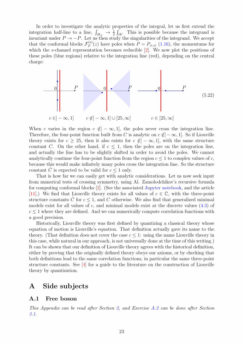
invariant under P → −P . Let us then study the singularities of the integrand. We acceptthat the conformal blocks F (s)

P (z) have poles when P = P〈r,s〉 (1.16), the momentums forwhich the s-channel representation becomes reducible [2]. We now plot the positions ofthese poles (blue regions) relative to the integration line (red), depending on the centralcharge:

P0 P0 P0

c ∈]−∞, 1] c /∈]−∞, 1] ∪ [25,∞[ c ∈ [25,∞[

(5.22)

When c varies in the region c /∈] − ∞, 1], the poles never cross the integration line.Therefore, the four-point function built from C is analytic on c /∈]−∞, 1]. So if Liouvilletheory exists for c ≥ 25, then it also exists for c /∈] − ∞, 1], with the same structureconstant C. On the other hand, if c ≤ 1, then the poles are on the integration line,and actually the line has to be slightly shifted in order to avoid the poles. We cannotanalytically continue the four-point function from the region c ≤ 1 to complex values of c,because this would make infinitely many poles cross the integration line. So the structureconstant C is expected to be valid for c ≤ 1 only.

That is how far we can easily get with analytic considerations. Let us now seek inputfrom numerical tests of crossing symmetry, using Al. Zamolodchikov’s recursive formulafor computing conformal blocks [2]. (See the associated Jupyter notebook, and the article[11].) We find that Liouville theory exists for all values of c ∈ C, with the three-pointstructure constants C for c ≤ 1, and C otherwise. We also find that generalized minimalmodels exist for all values of c, and minimal models exist at the discrete values (4.3) ofc ≤ 1 where they are defined. And we can numerically compute correlation functions witha good precision.

Historically, Liouville theory was first defined by quantizing a classical theory whoseequation of motion is Liouville’s equation. That definition actually gave its name to thetheory. (That definition does not cover the case c ≤ 1: using the name Liouville theory inthis case, while natural in our approach, is not universally done at the time of this writing.)It can be shown that our definition of Liouville theory agrees with the historical definition,either by proving that the originally defined theory obeys our axioms, or by checking thatboth definitions lead to the same correlation functions, in particular the same three-pointstructure constants. See [4] for a guide to the literature on the construction of Liouvilletheory by quantization.

A Side subjects

A.1 Free boson

This Appendix can be read after Section 2, and Exercise A.2 can be done after Section3.1.

23

We will now introduce the conformal field theory of the free boson. This provides thesimplest examples of a CFT with an extended symmetry algebra, i.e. an algebra that isstrictly larger than the Virasoro algebra: the abelian affine Lie algebra. This is a goodpreparation for Wess–Zumino–Witten models, with their non-abelian affine Lie algebras.

Just as the Virasoro algebra can be defined by the self-OPE of the energy-momentumtensor (2.13), we define the abelian affine Lie algebra by the self-OPE of a locally holo-morphic current J(y),

J(y)J(z) =y→z

−12

(y − z)2+O(1) . (A.1)

We are still doing conformal field theory, because we can build an energy-momentumtensor from the current. Actually, for any Q ∈ C, we can build a Virasoro algebra, whosegenerators are the modes of

T (y) = −(JJ)(y)−Q∂J(y) . (A.2)

We choose a value of Q, and assume that the resulting Virasoro algebra generates confor-mal transformations, and in particular obeys Axiom 2.3. Given the behaviour (2.10) ofT (y) at infinity, we assume

J(y) =y→∞

Q

y+O

(

1

y2

)

. (A.3)

Definition A.1 (Normal-ordered product)Given two locally holomorphic fields, their normal-ordered product is

(AB)(z) =1

2πi

∮

z

dy

y − zA(y)B(z) . (A.4)

Equivalently, if A(y)B(z) is the singular part of the OPE A(y)B(z), we have

(AB)(z) = limy→z

(

A(y)B(z)−A(y)B(z))

, (A.5)

A(y)B(z) = A(y)B(z) + (AB)(z) +O(y − z) . (A.6)

The normal-ordered product is neither associative, nor commutative.

OPEs that involve normal-ordered products can be computed using Wick’s theorem,

A(z)(BC)(y) =z→y

1

2πi

∮

y

dx

x− y

(

A(z)B(x)C(y) +B(x)A(z)C(y))

. (A.7)

For example, we can compute

(JJ)(y)J(z) =z→y

− J(y)

(y − z)2+O(1) =

y→z− ∂

∂z

J(z)

y − z+O(1) , (A.8)

which leads to

T (y)J(z) =y→z

−Q

(y − z)3+

∂

∂z

1

y − zJ(z) +O(1) . (A.9)

Then we can compute the OPE T (y)T (z), and we find the OPE (2.13), where the centralcharge is given by c = 1 + 6Q2 (repeating eq. (1.12)).

24

We define an affine primary field with the momentum α by the OPE

J(y)Vα(z) =y→z

α

y − zVα(z) +O(1) . (A.10)

Using Wick’s theorem, we deduce

T (y)Vα(z) =y→z

α(Q− α)

(y − z)2Vα(z)−

2α

y − z(JVα)(z) +O(1) . (A.11)

This means that our affine primary field is also a Virasoro primary field with the conformaldimension α(Q− α), and that

∂Vα(z) = −2α(JVα)(z) . (A.12)

Knowing its poles and residues, we compute⟨

J(y)

N∏

i=1

Vαi(zi)

⟩

=

N∑

i=1

αi

y − zi

⟨

N∏

i=1

Vαi(zi)

⟩

. (A.13)

From eq. (A.3) we first deduce the global Ward identity

(

∑Ni=1 αi −Q

)

⟨

N∏

i=1

Vαi(zi)

⟩

= 0 , (A.14)

which means that the momentum is conserved. Then, using eq. (A.12), we deduce(

∂

∂zi+∑

j 6=i

2αiαj

zi − zj

)⟨

N∏

i=1

Vαi(zi)

⟩

= 0 . (A.15)

(This is the abelian version of the Knizhnik–Zamolodchikov equation.) We can solve thisdifferential equation, and we find

⟨

N∏

i=1

Vαi(zi)

⟩

∝ δ(

∑Ni=1 αi −Q

)

∏

i<j

(zi − zj)−2αiαj . (A.16)

Affine symmetry determines the zi-dependence of all correlation functions, while Virasorosymmetry did it only for two- and three-point functions.

Exercise A.2 (Free bosonic spectrums)In the case c = 1, we want to build CFTs with the abelian affine Lie algebra symmetry,whose primary states include diagonal states and non-diagonal states with integer spins.We interpret momentum conservation as implying that the spectrum is closed under theaddition of momentums. Let ( i

2R, i2R) be the left and right momentums of a diagonal

primary state, and (α, α) the momentums of another state. Show that

i

R(α− α) ∈ Z . (A.17)

Under mild assumptions, deduce that the spectrum is of the type

SR =⊕

(n,w)∈Z2

U i2(

nR+Rw) ⊗ U i

2(nR−Rw) , (A.18)

where Uα is the representation of the abelian affine Lie algebra that corresponds to theprimary field Vα. The corresponding CFT is called the compactified free boson, with thecompactification radius R. Do compactifield free bosons exist for c 6= 1?

25

A.2 Modular bootstrap

This Appendix can be read after Section 4.1.

The torus zero-point function (or partition function) is a correlation function that onlydepends on the spectrum, and on characters of representations of the Virasoro algebra.Since there is no dependence on three-point structure constants, and since characters aremuch simpler than four-point blocks, the torus partition function is much simpler thanfour-point functions on the sphere. Nevertheless, the partition function obeys a nontrivialconstraint called modular invariance.

Definition A.3 (Modular bootstrap)The modular bootstrap consists in using the modular invariance of the torus partitionfunction for deriving constraints on the spectrum.

However, modular invariant partition functions do not always correspond to consistentCFTs: consistency of a CFT on all Riemann surfaces is equivalent to crossing symmetryof the sphere four-point function and modular invariance of the torus one-point function[7]. And some CFTs are consistent on the sphere only.

Definition A.4 (Torus partition function)For a CFT with the spectrum S, the partition function on the torus C

Z+τZis

Z(τ) = TrS qL0− c

24 qL0− c24 where q = e2πiτ . (A.19)

Axiom A.5 (Modular invariance)For ( a b

c d ) ∈ SL2(Z), the torus partition function is invariant under the correspondingmodular transformation,

Z(τ) = Z

(

aτ + b

cτ + d

)

. (A.20)

Let us give some justification for the definition of the torus partition function. The energyoperator on the complex plane is L0 + L0: under the conformal map z 7→ log z to theinfinite cylinder, this becomes L0 + L0 − c

12. To get the torus, we truncate the cylinder

to a finite length i(τ − τ ), and identify points on the upper and lower boundaries after arotation by τ + τ . The partition function is the trace of the operator that performs thisidentification.

z

i(L0 − L0)

L0 + L0

log z

i(L0 − L0)

L0 + L0 − c12

τ + τ

i(τ − τ )

complex plane infinite cylinder torus

26

Actually, modular invariance reduces to the invariance under two particular modulartransformations,

T (τ) = τ + 1 , S(τ) = −1

τ. (A.21)

The condition Z(τ) = Z(τ + 1) amounts to L0 − L0 having integer eigenvalues, in otherwords all states having integer conformal spins. The condition Z(τ) = Z(− 1

τ) is more

complicated: to exploit this condition, let us decompose the spectrum into factorizedrepresentations of the type R⊗ R′. The contribution of R⊗ R′ to the partition functionis χR(τ)χR′(−τ ), where we define the character of a representation as

χR(τ) = TrR qL0− c24 . (A.22)

From Z(τ) = Z(− 1τ), we first deduce that there exists a modular S-matrix such that

χR(τ) =∑

R′

SR,R′χR′(− 1τ) . (A.23)

Let us consider a diagonal CFT, with the partition function Z(τ) =∑

R χR(τ)χR(−τ ).Comparing two expressions for Z(− 1

τ),

Z(− 1τ) =

∑

R′,R′′

∑

RSR,R′SR,R′′χR′(− 1

τ)χR′′( 1

τ) =

∑

RχR(− 1

τ)χR(

1τ) , (A.24)

we deduce SST = Id. Since S2 = Id by construction, this means that a diagonal modularinvariant partition function exists if and only if the S-matrix is symmetric. (This rea-soning must be modified in CFTs based on larger symmetry algebras [5]. In particular,characters depend not just on τ but on extra variables, and S2 is no longer identity butthe charge conjugation matrix, where charge conjugation is the involution R → R∗ suchthat 〈VRVR∗〉 6= 0.)

Let us compute the characters and modular S-matrix of minimal models. We startwith the character of a Verma module with momentum P ,

χP (τ) =q−P 2

η(τ)with η(τ) = q

1

24

∞∏

n=1

(1− qn) , (A.25)

where the nontrivial factor is called the Dedekind η function. Why this function? If L−1

was our only creation mode, we would have one state at each level, and the characterwould be χ(τ) ∼ 1 + q + q2 + q3 + · · · = 1

1−q. If we had L−2 instead, the character would

be χ(τ) ∼ 11−q2

. And in order to count the states that come from two creation modes, wemust multiply the corresponding series.

In order to compute the character of a degenerate representation, we should subtractthe contributions of null vectors and their descendent states. For a simply degeneraterepresentation, the character is therefore

χ〈r,s〉(τ) = χP〈r,s〉(τ)− χP〈r,−s〉(τ) . (A.26)

For a fully degenerate representation in the Kac table of the (p, q) minimal model, thestructure is a bit more complicated: we have to subtract the two null vectors and theirdescendents, but add again the intersection of their two Verma submodules, which wassubtracted twice. It turns out that the corresponding S-matrix is symmetric, showingthat the A-series minimal models have modular invariant partition functions. Actually,the D-series minimal models too.

27

Exercise A.6 (Characters of minimal models)Show that the characters of fully degenerate representations in the Kac table of the (p, q)minimal model are

χ〈r,s〉(τ) =∑

k∈Z

(

χP〈r,s〉+ik√pq − χP〈r,−s〉+ik

√pq

)

. (A.27)

Exercise A.7 (Modular S-matrices of minimal models)Show that the modular S-matrix of the (p, q) minimal model is

S〈r,s〉,〈r′,s′〉 = −√

8

pq(−1)rs

′+r′s sin

(

πq

prr′)

sin

(

πp

qss′)

. (A.28)

B Solutions of Exercises

Exercise 1.1. Let us introduce the map

g =

(

a bc d

)

∈ GL2(C) 7−→ fg(z) =az + b

cz + d. (B.1)

A direct calculation shows that fg1 ◦ fg2 = fg1g2, so that our map is a group morphismfrom GL2(C) to the global conformal group of the sphere. The morphism is manifestlysurjective, let us determine its kernel. The matrix g belongs to the kernel if and only if

az+bcz+d

= z, equivalently g =

(

a 00 a

)

for a ∈ C∗. So the global conformal group can be

written as GL2(C)C∗ . Now, modulo C∗, any element of GL2(C) is equivalent to a matrix of

determinant one, i.e. an element of SL2(C). So the map g 7−→ fg is also surjective asa map from SL2(C) to the global conformal group, and in SL2(C) its kernel is Z2, since

det

(

a 00 a

)

= 1 ⇐⇒ a ∈ {1,−1}. Therefore, the global conformal group can also be

written as SL2(C)Z2

.

Exercise 1.3. Let us look for central extensions of the Witt algebra, starting with theansatz

[1, Ln] = 0 , [Ln, Lm] = (n−m)Ln+m + f(n,m)1 , (B.2)

for some function f(n,m). The constraint on f(n,m) from antisymmetry [Ln, Lm] =−[Lm, Ln] is

f(n,m) = −f(m,n) . (B.3)

The constraint from the Jacobi identity [[Ln, Lm], Lp] + [[Lm, Lp], Ln] + [[Lp, Ln], Lm] = 0is

(n−m)f(n +m, p) + (m− p)f(m+ p, n) + (p− n)f(n+ p,m) = 0 . (B.4)

In the case p = 0, this reduces to

(m+ n)f(n,m) + (m− n)f(m+ n, 0) = 0 . (B.5)

This means that for m+ n 6= 0, f(n,m) can be written in terms of a function of only onevariable. We can actually set this function to zero by reparametrizing the generators ofour algebra. If indeed we define

Ln = L′n + g(n)1 , (B.6)

28

for some function g(n), then the generators L′n obey commutation relations of the type

(B.2), with however the function

f ′(n,m) = f(n,m) + (n−m)g(n+m) . (B.7)

Let us choose g(n) = −f(n,0)n

for n 6= 0, then eq. (B.5) becomes f ′(n,m) = 0 for n+m 6= 0.We therefore write

f ′(n,m) = δn+m,0h(n) , (B.8)

for some unknown function h(n) such that h(0) = 0 by antisymmetry. We still have thefreedom to choose g(0), with f ′(n,−n) = f(n,−n) + 2ng(0). We use this freedom forsetting h(1) = 0. Let us rewrite the Jacobi identity (B.4) in terms of the function h(n):

(n−m)h(m+ n)− (2m+ n)h(n) + (m+ 2n)h(m) = 0 . (B.9)

In the particular case m = 1, this becomes (n − 1)h(n + 1) − (n + 2)h(n) = 0. Sinceh(−1) = h(0) = h(1) = 0 it is natural to write h(n) = (n − 1)n(n + 1)h′(n), and ourequation becomes h′(n+1) = h′(n). This shows that h(n) = λn(n2−1) for some constantλ. To conclude, it remains to check that this solves eq. (B.9) not only for m = 1, but forall values of m – a straightforward computation.

Exercise 1.7. Straighforward calculations.

Exercise 2.8. As a consequence of eq. (2.8) together with T (y)T (z) = T (z)T (y), wehave

[L(z0)n , L(z0)

m ] = − 1

4π2

(∮

z0

dy

∮

z0

dz −∮

z0

dz

∮

z0

dy

)

(y − z0)n+1(z − z0)

m+1T (y)T (z) ,

(B.10)

In this formula,∮

z0dy∮

z0dz means that the integration over z should be performed before

the integration over y, so the contour of integration over z should be inside the contourof integration over y. We have a second term where the positions of the contours areexchanged. Let us focus on the contribution of a given value of z: in the second term thisis simply

∮

z0dy, while in the first term this is

∮

zdy +

∮

z0dy. Therefore, we find

∮

z0

dy

∮

z0

dz −∮

z0

dz

∮

z0

dy =

∮

z0

dz

∮

z

dy , (B.11)

and therefore,

[L(z0)n , L(z0)

m ] = − 1

4π2

∮

z0

dz

∮

z

dy (y − z0)n+1(z − z0)

m+1T (y)T (z) . (B.12)

Let us compute the integral over y, using the OPE (2.13). We find

1

2πi

∮

z

dy (y − z0)n+1T (y)T (z) =

c

12n(n2 − 1)(z − z0)

n−2

+ 2(n+ 1)(z − z0)nT (z) + (z − z0)

n+1∂T (z) . (B.13)

It remains to perform the integration over z. Using eq. (2.8), this shows that [L(z0)n , L

(z0)m ]

is given by the Virasoro algebra’s commutation relations, with the last two terms of eq.(B.13) contributing respectively (2n+ 2)L

(z0)m+n and −(m+ n + 2)L

(z0)m+n.

29

Exercise 2.9. If⟨

V∆(z1)V∆(z2)⟩

= (z1 − z2)−2∆, then

⟨

V∆(∞)V∆(z2)⟩

= limz→∞

z2∆(z − z2)−2∆ = 1 . (B.14)

Similarly, we compute⟨

V∆1(∞)V∆2

(z2)V∆3(z3)

⟩

∝ (z2 − z3)∆1−∆2−∆3 . (B.15)

And the computation for the four-point function is straightforward.Using eq. (2.17) with ( a b

c d ) = ( 0 −11 0 ), we find

⟨

N∏

i=1

V∆i

(

− 1zi

)

⟩

=

N∏

i=1

z2∆i

i

⟨

N∏

i=1

V∆i(zi)

⟩

. (B.16)

Since V∆1(− 1

z1) has a finite limit as z1 → ∞, we deduce that z2∆1

1 V∆1(z1) has a finite limit

too, provided z2, . . . , zN are finite.

Exercise 2.10. Straightforward calculations lead to⟨

V〈2,1〉V∆2V∆3

⟩

6= 0 =⇒ 2(∆2 −∆3)2 + b2(∆2 +∆3)− 2∆2

〈2,1〉 − b2∆〈2,1〉 = 0 .

(B.17)

It only remains to replace conformal dimensions with momentums.

Exercise 2.11. The calculations using eq. (2.21) are straightforward but tedious. Letus try to do a bit better. What prevents us from directly applying the BPZ equation

to G(z) =⟨

V〈2,1〉(z)V∆1(0)V∆2

(∞)V∆3(1)⟩

, is that the equation involves derivatives with

respect to the three positions that we want to set to fixed values. So apparently we need

to introduce⟨

V〈2,1〉(z)V∆1(z1)V∆2

(z2)V∆3(z3)

⟩

. However, using the global Ward identities,

any derivative with respect to z1, z2, z3 can be rewritten as a derivative with respect toz, and therefore eliminated from the BPZ equation. To do this efficiently, rememberthat the derivatives with respect to zi originated from using eq. (2.24) for computing⟨

L−2V〈2,1〉(z)V∆1(z1)V∆2

(z2)V∆3(z3)

⟩

. In order to eliminate such derivatives, it is enough

to compute the following expression instead:

1

2πi

∮

z

dy

∏3i=1(y − zi)

y − zZ(y) . (B.18)

Closing the contour on y = z gives us a combination of L(z)−2,

∂∂z, and scalar factors,

acting on⟨

V〈2,1〉(z)V∆1(z1)V∆2

(z2)V∆3(z3)

⟩

. Closing the contour on y = zi instead does

not produce any derivatives with respect to zi, thanks to the vanishing of the prefactor∏3

i=1(y−zi)

y−zat y = zi. This leads to a version of the BPZ equation that involves derivatives

with respect to z only:{

3∏

i=1

(z − zi)

(

− 1

b2∂2

∂z2+

3∑

i=1

1

z − zi

∂

∂z

)

+ (3z − z1 − z2 − z3)∆〈2,1〉

+z12z13z1 − z

∆1 +z21z23z2 − z

∆2 +z31z32z3 − z

∆3

}

⟨

V〈2,1〉(z)

3∏

i=1

V∆i(zi)

⟩

= 0 . (B.19)

In this version of the BPZ equation, it is straightforward to send z1, z2, z3 to 0,∞, 1, andwe obtain eq. (2.30).

30

Exercise 3.5. Let us insert∮

Cdz(z−z2)

2T (z) on both sides of eq. (3.5), for C a contouraround both z1 and z2. Neglecting the dependence on zi, we rewrite this OPE as

V∆1(z1)V∆2

(z2) =∑

∆∈SC∆1,∆2,∆z

∆−∆1−∆2

12

(

V∆(z2) + fz12L−1V∆(z2) +O(z212))

. (B.20)

We first compute the left-hand side. The integrand (z−z2)2T (z)V∆1

(z1)V∆2(z2) is regular

at z = z2, and we only pick contributions from the pole at z = z1. Using the OPET (z)V∆1

(z1) (2.9), we find

1

2πi

∮

C

dz(z − z2)2T (z)V∆1

(z1)V∆2(z2) =

(

2z12∆1 + z212∂

∂z1

)

V∆1(z1)V∆2

(z2) . (B.21)

Using the OPE (3.5), we compute

1

2πi

∮

C

dz(z − z2)2T (z)V∆1

(z1)V∆2(z2)

=∑

∆∈SC∆1,∆2,∆z

∆−∆1−∆2+112

(

(∆ +∆1 −∆2)V∆(z2) +O(z12))

. (B.22)

Now we insert∮

Cdz(z−z2)

2T (z) on the right-hand side of eq. (3.5)For any field V (z2) (pri-mary or descendent) we have 1

2πi

∮

Cdz(z−z2)

2T (z)V (z2) = L1V (z2). Since L1V∆2(z2) = 0,

the leading contribution is from the level one descendent L−1V∆2(z2),

1

2πi

∮

C

dz(z − z2)2T (z)V∆1

(z1)V∆2(z2)

=∑

∆∈SC∆1,∆2,∆z

∆−∆1−∆2+112

(

fL1L−1V∆(z2) +O(z12))

. (B.23)

Using L1L−1V∆(z2) = 2∆V∆(z2), and comparing with the left-hand side result (B.22),this leads to

f =∆+∆1 −∆2

2∆. (B.24)

Of course, this expression is also the coefficient of the right-moving descendent L−1V∆(z2).

Exercise 3.6. Let us write the OPE (3.5) in the case of the degenerate field V〈1,1〉, whileomitting the dependence on zi:

V〈1,1〉(z1)V∆2(z2) =

∑

∆∈SC〈1,1〉,∆2,∆

∞∑

i=0

z∆−∆2+i12 LiV∆(z2) , (B.25)

where LiV∆(z2) is some descendent at level i, and L0V∆(z2) = V∆(z2). Since∂

∂z1V〈1,1〉(z1) =

0, we have

0 =∑

∆∈SC〈1,1〉,∆2,∆

∞∑

i=0

z∆−∆2+i−112 (∆−∆2 + i)LiV∆(z2) . (B.26)

Assuming C〈1,1〉,∆2,∆ 6= 0, the vanishing of the leading i = 0 term implies ∆2 = ∆. Thevanishing of an i > 0 term then implies LiV∆(z2) = 0. Therefore, the OPE reduces to

V〈1,1〉(z1)V∆(z2) = C∆V∆(z2) , (B.27)

where C∆ = C〈1,1〉,∆,∆. Let us use this OPE in a correlation function that involves thefields V〈1,1〉(z1)V∆2

(z2)V∆3(z3). Using commutativity and associativity of the OPE, we

obtain

V〈1,1〉(z1)V∆2(z2)V∆3

(z3) = C∆2V∆2

(z2)V∆3(z3) = C∆3

V∆2(z2)V∆3

(z3) . (B.28)

This implies C∆2= C∆3

, and actually C∆ cannot depend on ∆.

31

Exercise 3.8. Using the OPE (3.5) including the first subleading correction from Ex-ercise 3.5, and omitting the dependence on zi, we have

⟨

V∆1(z)V∆2

(0)V∆3(∞)V∆4

(1)⟩

=∑

∆∈SC∆1,∆2,∆z

∆−∆1−∆2

×⟨(

1 +∆+∆1 −∆2

2∆zL−1 +O(z2)

)

V∆(0)V∆3(∞)V∆4

(1)

⟩

. (B.29)

Let us then compute⟨

L−1V∆(0)V∆3(∞)V∆4

(1)⟩

. This is done by computing it for three

arbitrary field positions before specializing to 0, 1,∞, using L−1V∆(z) = ∂∂zV∆(z). The

result is⟨

L−1V∆(0)V∆3(∞)V∆4

(1)⟩

= C∆,∆3,∆4(∆ +∆4 −∆3) . (B.30)

We therefore deduce

⟨

V∆1(z)V∆2

(0)V∆3(∞)V∆4

(1)⟩

=∑

∆∈SC∆1,∆2,∆C∆,∆3,∆4

z∆−∆1−∆2

×(

1 +(∆ +∆1 −∆2)(∆ +∆4 −∆3)

2∆z +O(z2)

)

, (B.31)

which is equivalent to eq. (3.13). The first subleading term has a pole at ∆ = 0, with theresidue (∆1 −∆2)(∆4 −∆3). The residue vanishes if ∆1 = ∆2 or ∆3 = ∆4, i.e. if at leastone of the three-point functions

⟨

V〈1,1〉V∆1V∆2

⟩

and⟨

V〈1,1〉V∆3V∆4

⟩

is non-vanishing.

Exercise 3.12. We already know that the fusion product (3.25) holds for the represen-tations R〈1,1〉, R〈2,1〉 and R〈1,2〉. Let us prove it more generally by recursion on r, s. Letus assume that it holds for all r ≤ r0 and s ≤ s0. For s ≤ s0 we compute

R〈2,1〉 ×R〈r0,s〉 × VP =

r0−1

2∑

i=− r0−1

2

s−1

2∑

j=− s−1

2

R〈2,1〉 × VP+ib+jb−1 , (B.32)

=

r02∑

i=− r02

+

r0−2

2∑

i=− r0−2

2

s−1

2∑

j=− s−1

2

VP+ib+jb−1 . (B.33)

= R〈r0−1,s〉 × VP +

r02∑

i=− r02

s−1

2∑

j=− s−1

2

VP+ib+jb−1 . (B.34)

(This is true even if r0 = 1, with the convention R〈0,s〉 = 0.) We obtain a combinationof finitely many Verma modules, which shows that R〈2,1〉 × Rr0,s must be a degeneraterepresentation. In this degenerate representation, we know that the highest-weight stateshave the momentums P〈r0,s〉± b

2= P〈r0±1,s〉. We already know that the momentum P〈r0−1,s〉

corresponds to the degenerate representation R〈r0−1,s〉, and there must be a degeneraterepresentation with the momentum P〈r0+1,s〉, which we call R〈r0+1,s〉. We can similarly dothe recursion on s, and we obtain degenerate representations R〈r,s〉 with r, s ∈ N∗.

The same method can be used for determining the fusion products (3.26) of degen-erate representations by recursion on r1, s1, starting with the known cases (r1, s1) ∈{(1, 1), (2, 1), (1, 2)}.

32

Exercise 4.5. Let R〈r1,s1〉 and R〈r2,s2〉 be two doubly degenerate representations inSp,q. The fusion product R〈r1,s1〉 × R〈r2,s2〉 must be a subspace of two fusion productscomputed with the rule (3.26) for degenerate representations: R〈r1,s1〉 × R〈r2,s2〉 andR〈r1,s1〉 × R〈p−r2,q−s2〉. The determination of this subspace is not completely straight-forward, because each representation that appears in one of our two fusion products canbe written in two possible ways, R〈r3,s3〉 or R〈p−r3,q−s3〉. This ambiguity can be liftedby writing the two fusion products such that the parities of r3, s3 are the same in onefusion products as in the other. (Remember that at least one of the integers p, q mustbe odd.) In particular, if we write R〈r1,s1〉 ×R〈r2,s2〉 as in eq. (3.26), we should not writeR〈r1,s1〉 ×R〈p−r2,q−s2〉 as

R〈r1,s1〉 ×R〈p−r2,q−s2〉 =

r1−r2+p−1∑

r32=|r1+r2−p|+1

s1−s2+q−1∑

s32=|s1+s2−q|+1

R〈r3,s3〉 , (B.35)

but rather as

R〈r1,s1〉 ×R〈p−r2,q−s2〉 =

min(r1+r2,2p−r1−r2)−1∑

r32=r2−r1+1

min(s1+s2,2q−s1−s2)−1∑

s32=s2−s1+1

R〈r3,s3〉 . (B.36)

In this form, we see that the intersection of the two fusion products R〈r1,s1〉×R〈r2,s2〉 andR〈r1,s1〉 ×R〈p−r2,q−s2〉 of degenerate representations is given by eq. (4.7). Taking furtherintersections withR〈p−r1,q−s1〉×R〈r2,s2〉 andR〈p−r1,q−s1〉×R〈p−r2,q−s2〉 does not yield furtherconstraints, and the fusion products of our doubly degenerate representations are thereforegiven by eq. (4.7).

Exercise 4.8. Fusion rules are a priori defined for representations of the Virasoro al-gebra, and do not know how the left- and right-moving representations are combined.Therefore, fusion rules may not unambiguously determine operator product expansionsin models where the same left-moving Virasoro representation is combined with differentright-moving representations.

However, assuming that p is even, let us look at the values of the r index in the D-series spectrum (4.10). The parity of r is unambiguously defined, as it does not changeunder (r, s) → (p − r, q − s). If moreover p ≡ 0 mod 4, then r takes odd values in thediagonal sector, and even values in the non-diagonal sector: therefore, the two sectors donot involve the same representations of the Virasoro algebra. From the fusion product(4.7), we deduce that the fusion product of two representations is diagonal if and only ifthe two representations belong to the same sector. Let us write this in terms of OPEs ofthe primary fields V ǫ

〈r,s〉 of the model, where the boolean ǫ = r − 1 mod 2 indicates the

sector: V 0〈r,s〉 corresponds to the representation R〈r,s〉⊗R〈r,s〉, and V 1

〈r,s〉 to R〈r,s〉⊗R〈p−r,s〉.We then have OPEs of the type

V ǫ1〈r1,s1〉V

ǫ2〈r2,s2〉 ∼

min(r1+r2,2p−r1−r2)−1∑

r32=|r1−r2|+1

min(s1+s2,2q−s1−s2)−1∑

s32=|s1−s2|+1

V ǫ1+ǫ2〈r3,s3〉 . (B.37)

For p ≡ 2 mod 4, we still use the boolean ǫ for labelling sectors, although it is no longerrelated to the parity of r, as r is odd in both sectors. The same expression for the fusionrules makes sense, although the conservation of diagonality is now an ansatz to be tested,rather than an unavoidable consequence of symmetry.

33

Exercise 5.3. From eq. (5.16), we deduce how the function Υb(x) behaves under shifts:

Υb(x+ b)

Υb(x)= λ2bx−1

b

∞∏

n=0

[

n + 1− bx

n+ bxe

∑∞m=0

2bx−1

(Q2+mb+nb−1)

2

]

. (B.38)

From Weierstrass’s definition of the Gamma function, we deduce the product formula

γ(x) = e−γEM(2x−1)1− x

x

∞∏

n=1

[

n+ 1− x

n+ xe

2x−1

n

]

, (B.39)

where γEM is the Euler–Mascheroni constant. This implies

Υb(x+ b)

Υb(x)= γ(bx)e(2bx−1)(log λb+γEM+Kb) , (B.40)

where we define

Kb =

∞∑

n=0

[ ∞∑

m=0

1(

Q

2+mb+ nb−1

)2 − 1

n

]

, (B.41)

with the convention 10= 0. We are not there yet, because Kb is not invariant under b → 1

b.

To understand its behaviour under b → 1b, we introduce a cutoff M on the sum over M ,

and perform the split∑∞

n=0 =∑M

n=0+∑∞

n=M+1. This leads to

Kb −Kb−1 = limM→∞

[

M∑

n=0

∞∑

m=M+1

−M∑

m=0

∞∑

n=M+1

]

1(

Q

2+mb+ nb−1

)2 . (B.42)

In order to compute this limit, we can replace the sums with integrals, and we obtain

Kb −Kb−1 = limM→∞

[

∫ Mb−1

0

dy

∫ ∞

Mb

dx−∫ Mb

0

dx

∫ ∞

Mb−1

dy

]

1

(x+ y)2= −2 log b . (B.43)

This shows that Kb + log b is invariant under b → 1b. Therefore, we set

λb = e−γEM−Kb−log b , (B.44)

and we obtain the shift equation (5.13) for Υb(x+b)Υb(x)

. Since λb is invariant under b → 1b, the

shift equation forΥb(x+

1

b)

Υb(x)follows immediately.

Exercise A.2. For c = 1 the conformal dimension is related to the momentum by∆ = −α2. If we have a state with momentums (α, α), its spin is α2 − α2 ∈ Z. Since wealso assume that the spectrum is closed under fusion, and that we have a diagonal statewith momentums ( i

2R, i2R), we must have a state with momentums (α+ i

2R, α+ i

2R). The

condition for this state to have integer spin is

(

α + i2R

)2 −(

α + i2R

)2 ∈ Z ⇐⇒ i

R(α− α) ∈ Z . (B.45)

We assume that there are nondiagonal states (α, α) that minimize this number, i.e. α−α =−iR. Since we also have α2 −α2 = −(α− α)(α+ α) ∈ Z, we deduce α+ α ∈ i

RZ. Again,

we assume that all allowed values actually occur, so that there is a state with α+ α = 0,i.e. a state with momentums (− iR

2, iR

2).

34

For (α, α) any state, the condition for the spin of (α − iR2, α + iR

2) to be integer is

iR(α + α) ∈ Z. Adding the constraint (B.45), we deduce that our state must belong tothe spectrum SR (A.18).

For an arbitrary central charge, the conformal dimension is ∆ = α(Q − α), andcondition for a state in the spectrum SR to have integer spin is

Q(α− α) ∈ Z ⇐⇒ QiRw ∈ Z . (B.46)

This must hold for any w ∈ Z, and we must have R ∈ iQZ. Therefore, compactified free

bosons exist only for certain discrete values of the radius.

Exercise A.6. To do this exercise, we only need to know the identities

∆〈r,s〉 = ∆〈−r,−s〉 = ∆〈p+r,q+s〉 , (B.47)

and the fact that a primary state with dimension ∆〈r,s〉 with r, s ∈ N∗ has a null vectorwith dimension ∆〈r,−s〉.

By definition, the doubly degenerate representation R〈r,s〉 = R〈p−r,q−s〉 has two van-ishing null vectors, with the dimensions ∆〈r,−s〉 and ∆〈p−r,s−q〉. Actually it has infinitelymany null vectors due to the identities (B.47), but we only consider the two null vectorswith the lowest conformal dimensions for the moment. The null vector with dimension∆〈r,−s〉 = ∆〈p+r,q−s〉 = ∆〈p−r,q+s〉 itself has null vectors with dimensions ∆〈p+r,s−q〉 and∆〈p−r,−q−s〉. One way to tame this proliferation of null vectors is to use the identities(B.47) in order to rewrite them all with the same first index r, and to label them by theirsecond index. In this notation, the primary state s has null vectors −s and 2q − s. Thefirst one of these null vectors itself has null vectors s − 2q and 2q + s. Interestingly, thesecond null vector has two null vectors with the very same labels s− 2q and 2q + s. Weassume that two null vectors with the same conformal dimension are actually identical:this means that the submodules generated by the null vectors −s and 2q − s share twosubmodules. The character of our representation therefore starts with

χ〈r,s〉 = χs − χ−s − χ−s+2q + χs−2q + χs+2q + · · · , (B.48)

where χs is a temporary notation for the Verma module character χP〈r,s〉 , and the twoshared submodules had to be added back. Iterating the reasoning, we find

χ〈r,s〉 =∑

k∈Z(χs+2kq − χ−s+2kq) . (B.49)

Using P〈r,s+2q〉 = P〈r,s〉 + i√pq, this can be rewritten as eq. (A.27).

But what do we do with the infinitely many null vectors that we have neglected?Actually, nothing: the neglected null vectors all coincide with null vectors that we alreadydid take into account, and do not affect the character.

Exercise A.7. From the Fourier transforms of Gaussian functions, we deduce the mod-ular transformation of the character χP (τ) of a Verma module:

χP (τ) =√2i

∫

iR

dP ′ e4πiPP ′χP ′(− 1

τ) . (B.50)

Using the Poisson resummation formula∑

k∈Z e2πikx =

∑

ℓ∈Z δ(x+ ℓ), we then deduce themodular transformation of the characters of fully degenerate representation in the Kactable of the (p, q) minimal model,

χ〈r,s〉(τ) = −√

2

pq

∑

ℓ∈Zsin

(

πr

pℓ

)

sin

(

πs

qℓ

)

χi ℓ2√

pq(− 1

τ) . (B.51)

35

Let us insert∑p−1

r=1(−1)rs′sin(

π q

prr′)

on both sides of this equation. We also insert an

analogous sum over s. The right-hand side is computed using the elementary identity

p−1∑

r=1

(−1)rs′sin

(

πq

prr′)

sin

(

πr

pℓ

)

= −p

2

∑

ǫ=±ǫδℓ≡ǫqr′+ps′ mod 2p , (B.52)

and it can then be written in terms of characters of fully degenerate representations,leading to eq. (A.28).

List of Exercises

0.1 Exercise (Update Wikipedia) . . . . . . . . . . . . . . . . . . . . . . . . . . 31.1 Exercise (Global conformal group of the sphere) . . . . . . . . . . . . . . . 41.3 Exercise (Uniqueness of the Virasoro algebra) . . . . . . . . . . . . . . . . 41.7 Exercise (Level two null vectors) . . . . . . . . . . . . . . . . . . . . . . . . 52.8 Exercise (Virasoro algebra and OPE) . . . . . . . . . . . . . . . . . . . . . 82.9 Exercise (Global conformal symmetry) . . . . . . . . . . . . . . . . . . . . 92.10 Exercise (Second-order BPZ equation for a three-point function) . . . . . . 102.11 Exercise (BPZ second-order differential equation) . . . . . . . . . . . . . . 103.5 Exercise (Computing the OPE of primary fields) . . . . . . . . . . . . . . . 123.6 Exercise (V〈1,1〉 is an identity field) . . . . . . . . . . . . . . . . . . . . . . . 123.8 Exercise (Computing conformal blocks) . . . . . . . . . . . . . . . . . . . . 133.12 Exercise (Higher degenerate representations) . . . . . . . . . . . . . . . . . 154.5 Exercise (Closure of minimal model spectrums under fusion) . . . . . . . . 174.8 Exercise (Fusion rules of D-series minimal models) . . . . . . . . . . . . . . 185.3 Exercise (Upsilon function) . . . . . . . . . . . . . . . . . . . . . . . . . . . 21A.2 Exercise (Free bosonic spectrums) . . . . . . . . . . . . . . . . . . . . . . . 25A.6 Exercise (Characters of minimal models) . . . . . . . . . . . . . . . . . . . 28A.7 Exercise (Modular S-matrices of minimal models) . . . . . . . . . . . . . . 28

References

[1] S. Migliaccio, S. Ribault (2017) [arXiv:1711.08916]The analytic bootstrap equations of non-diagonal two-dimensional CFT

[2] A. Zamolodchikov, A. Zamolodchikov (1990 book)Conformal Field Theory and Critical Phenomena in Two-Dimensional Systems

[3] S. Ribault (2014 review) [arXiv:1406.4290]Conformal field theory on the plane

[4] J. Teschner (2017 review) [arXiv:1708.00680]A guide to two-dimensional conformal field theory

[5] P. Di Francesco, P. Mathieu, D. Senechal (1997 book)Conformal field theory

[6] J. Cardy (2008 review) [arXiv:0807.3472]Conformal Field Theory and Statistical Mechanics

36

[7] G. W. Moore, N. Seiberg (1989)Classical and Quantum Conformal Field Theory

[8] M. R. Gaberdiel (2000 review) [arXiv:hep-th/9910156]An Introduction to conformal field theory

[9] V. B. Petkova (1988)Two-dimensional (Half) Integer Spin Conformal Theories With Central Charge c < 1

[10] A. B. Zamolodchikov, A. B. Zamolodchikov (1996) [arXiv:hep-th/9506136]Structure constants and conformal bootstrap in Liouville field theory

[11] S. Ribault, R. Santachiara (2015) [arXiv:1503.02067]Liouville theory with a central charge less than one

37