Lectures on Homology of Symbols

Mariusz Wodzicki

Notes taken byPaweł Witkowski

December 2006

Contents

1 The algebra of classical symbols 3

1.1 Local definition of the algebra of symbols . . . . . . . . . . . . . . . . . . . . . 31.2 Classical pseudodifferentials operators . . . . . . . . . . . . . . . . . . . . . . . 51.3 Statement of results . . . . . . . . . . . . . . . . . . . . . . . . . . . . . . . . . . 71.4 Derivations of the de Rham algebra . . . . . . . . . . . . . . . . . . . . . . . . . 71.5 Koszul-Chevalley complex . . . . . . . . . . . . . . . . . . . . . . . . . . . . . . 121.6 A relation between Hochschild and Lie algebra homology . . . . . . . . . . . 131.7 Poisson trace . . . . . . . . . . . . . . . . . . . . . . . . . . . . . . . . . . . . . . 15

1.7.1 Graded Poisson trace . . . . . . . . . . . . . . . . . . . . . . . . . . . . . 171.8 Hochschild homology . . . . . . . . . . . . . . . . . . . . . . . . . . . . . . . . 181.9 Cyclic homology . . . . . . . . . . . . . . . . . . . . . . . . . . . . . . . . . . . 21

1.9.1 Further analysis of spectral sequence . . . . . . . . . . . . . . . . . . . 251.9.2 Higher differentials . . . . . . . . . . . . . . . . . . . . . . . . . . . . . 30

A Topological tensor products 32

B Spectral sequences 34

B.1 Spectral sequence of a filtered complex . . . . . . . . . . . . . . . . . . . . . . . 34B.2 Examples . . . . . . . . . . . . . . . . . . . . . . . . . . . . . . . . . . . . . . . . 37

2

Chapter 1

The algebra of classical symbols

1.1 Local definition of the algebra of symbols

Let X be a C∞-manifold (not necessarily compact), and E a vector bundle on X. Consider acoordinate patch

fU : U → X, U ⊂ Rn.

The cotangent bundle T∗X → X pulls back to U

T∗0 U //

π

²²

T∗U //

²²

T∗X

²²U U

fU // X

The bundle T∗0 U is defined as T∗U \ U. There is an isomorphism

T∗0 U ' //

π

²²

U × Rn0 ⊂ Rn × Rn

0

U

Using it we can denote the coordinates on T∗0 U by (u, ξ), where u = (u1, . . . , un) ∈ Rn

0 , andξ ∈ (ξ1, . . . , ξn) ∈ Rn.

To each open set U we associate a section aU := ∑∞j=0 aU

j , where each aUj is a section of

the bundle End(π∗ f ∗UE), where

π∗ f ∗UE

²²

// f •UE

²²

// E

²²T∗

0 U π // UfU // X

More precisely by aUm−j we denote the homogeneous part of degree m − j

aUm−j ∈ C∞(T∗

0 U, End(π∗ f ∗UE))(m − j).

There is a natural action of R∗+ on T∗

0 X given by t · (u, ξ) := (u, tξ). The infinitesimal actionis provided by the Euler field

Ξ =n

∑i=1

ξi∂ξi.

3

The homogenity condition for aUm−j is given by aU

m−j(u, tξ) = tm−jaUm−j(u, ξ).

The section aU belongs to the product

∞

∏j=0

C∞(T∗0 U, End(π∗ f ∗UE))(m − j)

which has a natural structure of Frechet space. With the norm

|ξ| :=√

ξ21 + . . . ξ2

n

we can write

|ξ|j−maUm−j ∈ C∞(T∗

0 U, End(π∗ f ∗UE))(0) ' C∞(S∗U, End(π∗ f ∗UE)),

where S∗U is the cosphere bundle T∗0 U/R∗

+π−→ U. The cotangent bundle T∗X → X is canon-

ically oriented and S∗X is canonically oriented (even though we do not have the orientationon X). Now S∗U is a canonically oriented (2n − 1)-manifold and S∗U ' U × Sn−1.

The sections aU are given locally, so we need a compatibility condition. We need a com-position law such that it will depend on all jets, not only on 1-jets as usual composition.

aU u bU : ∑α

δαξ aU D

[α]u bU

α = (α1, . . . , αn), αi ∈ N

Dui:=

1

i∂ui

, D[α]u =

1

α!Dα

u =1

α!i|α|∂α

u.

If aU is of order m, bU of order m′ using the notation for classical symbols

CSmU(U, E) :=

∞

∏j=0

(T∗0 U, End(π∗ f ∗UE))(m − j)

we can write

u : CSmU(U, E) × CSm′

U (U, E) → CSm+m′

U (U, E), m, m′ ∈ C.

Now suppose we have two open sets U, V ∈ Rn such that the images of charts fU : U → X,fV : V → X have nonempty intersection f (U) ∩ f (V). Denote

U′ := f −1U ( f (U) ∩ f (V)), V ′ := f −1

V ( f (U) ∩ f (V)),

fUV := f −1U fV : V ′ → U′.

For a smooth map f : X → Y there are induced maps

T f : TC → TY, (T f )x : (TX)x → (TY) f (x),

T f ∗ : T∗X → T∗Y, (T f )∗x : (T∗X)x ← (T∗Y) f (x).

Assume that T f is invertible

((T f )∗x)−1 : (TX)∗x → (TY)∗f (x)

4

Define a maps

X × TX → Y × TY, (x, v) 7→ ( f (x), (T f )x(v)),

X × T∗X → Y × T∗Y, (x, ξ) 7→ ( f (x), ((T f )∗)−1x (ξ)).

Now comes the question, to what extend aV and (T∗ f )∗aU agree? We have

aV = (T∗ f )∗(aU + (arbitrary high order correction terms))

= (T∗ fUV)∗(∑α

ψα∂αξ aU),

whereψα(u, ξ) = D

[α]z ei〈j>1

u (z), (T fUV )∗v(ξ)〉∣∣z=u, v=( f−1

V fU)(u),

j>1u (z) = f −1

V fU − j1U( f −1V fU),

so j>1u vanishes up to second order at point u ∈ U. The ψα(u, ξ) are scalar valued functions

on coordinate charts. They do not depend on symbols, only on manifold.In the whole notes we will be using a projective tensor product of topological vector

spaces desribed in the appendix (A).The product

CSm(X, E) × CSm′

(X, E) → CSm+m′

(X, E)

of Frechet spaces is associative. Define the algebra of symbols as

CS(X, E) : =⋃

m∈Z

CSm(X, E).

Let a := aU fU : U→X. The topology on CS(X, E) is defined as follows. We say that the netaλ converges to a symbol a if for any m ∈ C there exists λ0 such that aλ − a ∈ CSm(X, E)for all λ ≥ λ0.

The subalgebra CS0(X, E) is a Frechet algebra, and CS−j(X, E), j ∈ Z+ is a two sidedideal in CS0(X, E).

Remark 1.1. The multiplication

CSm(X, E) ⊗ CS(X, E) → CS(X, E)

is not continuous in both arguments.

1.2 Classical pseudodifferentials operators

Let A : C∞c (X, E) → C∞(X, E) be a pseudo differential operator. For a chart fU : U → X there

is an operatorf #U A : C∞

c (U, f ∗UE) → C∞(U, f ∗UE)

We can define it for ϕ ∈ C∞c (U, f ∗UE) as follows. First take (ϕ f −1

U )| f (supp ϕ), and then extendby 0, apply A and pullback, as in the following diagram

C∞c (X, E)

A // C∞(X, E)

f ∗U²²

C∞c (U, f ∗UE)

( fU)!

OO

f #U A

// C∞(U, f ∗UE)

5

Explicitly

( f #U A)ϕ(u) =

∫

Rnξ

∫

Uei〈u−u′, ξ〉β(u, u′, ξ)ϕ(u′)du′dξ + (Tϕ)(u),

where β ∈ C∞(U × T∗U, End(π∗ f ∗UE)) is called an amplitude,

β(u, u′, ξ) ∼∞

∑j=0

βm−j(u, u′, ξ),

βm−j(u, u′, tξ) = tm−jβ(u, u′, ξ),

T is a smoothing operator

(Tφ)(u) =

∫

UK(u, u′)ϕ(u′)|du′|,

and

|du| = |du1 ∧ · · · ∧ dun|, dξ =1

(2π)n|dξ1 ∧ · · · ∧ dξn|.

By CLm(X, E) we denote the space of classical pseudo differential operators, and by CLmprop(X, E)

the subset of operators which take functions with compact support into functions with com-pact support. For A ∈ CLm(X, E) there is a decomposition A = Aprop + S into a properpart Aprop and non proper smoothing part S. Define a Frechet space of arbitrary low orderoperators by

L−∞(X, E) :=⋂

m∈Z

CLm(X, E).

There is an isomorphism

CLm(X, E)/L−∞(X, E)'−→ CSm(X, E).

Classical symbols have a product

CLmprop(X, E) × CLm′

prop(X, E) → CLm+m′−1prop (X, E), m, m′ ∈ C.

We define the algebra of classical symbols as

CL(X, E) :=⋃

m∈Z

CLm(X, E).

The space of smoothing operators L∞(X, E) is defined as a kernel

L∞(X, E) ½ CL(X, E) ³ CS(X, E)

and if X is closed it is isomorphic (non canonically) to the space of rapidly decaying matrices

L−∞ = (aij)i,j=1...,∞ | |aij|(i + j)N → 0, as i + j → ∞.

This is the noncommutative orientation class of a closed manifold and index theorem is theway to state that. Index measures to what extend this sequence is not split.

The map

CL(X, E)/L−∞(X, E) → CS(X, E)

6

is defined as follows. For a classical pseudo differential operator

A : C∞c (X, E) → C∞(X, E)

we take the amplitude

βU(u, u′, ξ) ∼∞

∑j=0

βUm−j(u, u′, ξ)

and then define aU ∈ CS(X, E) by

aU :=(

e∑ni=1 ∂ξi

DuiβU

) ∣∣u=u′ .

1.3 Statement of results

The main goal is to compute the Hochschild and cyclic homology of the algebra of symbolsCS(X). Let T∗

0 X = T∗X \ X and Yc be the C∗-bundle over the cosphere bundle S∗X definedas

Yc := T∗0 X ×R+ C∗

C∗

²²S∗X

Theorem 1.2. There is a canonical isomorphism

HHq(CS(X)) ' H2n−qdR (Yc).

Regarding cyclic homology, consider on HCcontq (CS(X)) the filtration by the kernels of

the iterated S-map:

0 = Sq0 ⊂ Sq1 ⊂ . . . ⊂ Sqt = HCq(CS(X)),

where t =[ q

2

]and Sqr := ker S1+r

∗ ∩ HCq(CS(X)).

Theorem 1.3. The canonical map

I : HH•(CS(X)) → HC•(CS(X))

is injective. In particular

HCqr(CS(X)) = grSr HCq(CS(X)) := Sqr/Sq,r−1

is canonically isomorphic with

H2n−q+2rdR (Yc), r = 0, 1, . . . .

1.4 Derivations of the de Rham algebra

Let O be a commutative k-algebra with unit, and k any commutative ring of coefficients. Wedefine

Ω•O/k := Λ•

OΩ1O/k,

where Ω1O/k can be defined in a three ways:

7

• Serre’s pictureΩ1

O/k := I∆/I2∆,

where I∆ := ker(O⊗2 → O).

• Hochschild pictureΩ1

O/k := O⊗2/bO⊗3.

• Leibniz picture

Ω1O/k :=

O〈d f | f ∈ O〉

O〈d( f + g) − d f − dg, dc = 0 (c ∈ k), d( f g) − f dg − gd f 〉.

The differential d : O → Ω1O/k is defined in those three pictures as follows

• f 7→ d∆ f mod I2∆ = (1 ⊗ f − f ⊗ 1) mod I2

∆ (Serre’s picture),

• f 7→ d∆ f mod bO⊗3 = (1 ⊗ f − f ⊗ 1) mod bO⊗3 (Hochschild picture),

• f 7→ d f (Leibniz picture).

The derivation d∆ : O → I∆ ⊂ O⊗O is universal in the sense that if we have an O-bimoduleM and a derivation δ : O → M, then there exists a unique O-bimodule map δ such that thefollowing diagram commutes

M

Od //

δ

<<zzzzzzzzz

d∆ !!DDDD

DDDD

DI∆/I2

∆

δ

OOÂÂ

Â

I∆

OO

Let Derm(Ω•) = Dermk (Ω•) denote the algebra of degree m derivations, and

Der•(Ω•) :=⊕

m∈Z

Derm(Ω•).

If η is of degree p and ζ of degree q, then for δ ∈ Derm(Ω•) we have

δ(η ∧ ζ) = δ(η) ∧ ζ + (−1)pmη ∧ δ(ζ).

δ : Ωp → Ωp+m.

Furthermore Der•(Ω•) is a super Lie algebra, that is the commutators satisfy the super Jacobiidentity

0 = [[a, b], c] + (−1)|a|(|b|+|c|)[[b, c], a] + (−1)|c|(|a|+|b|)[[c, a], b].

Denote δp := δ|Ωp.

Proposition 1.4. The set Derm(Ω•) is naturally identified with the set of pairs (δ0, δ1), where

δ0 : O → Ωm

is a k-linear derivation of O with values in Ωm,

δ1 : Ω1 → Ωm+1

8

is a k-linear map such that

δ1( f α) = δ0( f ) ∧ α + f δ1(α).

and

δ1(α)α − (−1)m+1αδ1(α) = 0,

that is the super commutator [δ1(α), α] = 0.

Any derivation of degree m is uniquelly determined by δ0 and δ1. Thus Derm(Ω•) = 0for m < −1.

For δ0 = 0 we have

δ( f α1 ∧ · · · ∧ αp) =p

∑i=1

(−1)m(i−1) f α1 ∧ · · · ∧ δ1(αi) ∧ · · · ∧ αp.

Similarly for any φ ∈ HomO(Ω1, Ωm+1) there exists a corresponding derivation

δφ( f α1 ∧ · · · ∧ αp) :=p

∑i=1

(−1)m(i−1) f α1 ∧ · · · ∧ φ(αi) ∧ · · · ∧ αp.

Example 1.5. (The de Rham derivation) Let d0 = d : O → Ω1. Now we will give a construc-tion of d1 : Ω1 → Ω2. Consider a k-linear pairing

O ×O → Ω2, ( f , g) 7→ d f ∧ dg

O ×O //

²²

Ω2

O ⊗k O

;;vv

vv

v

O ×O //

²²

Ω2

(O ⊗k O)/I2∆

99rr

rr

r

Now we can take a restriction to I∆/I2∆ ⊂ (O ⊗k O)/I2

∆. Recall that I∆ consists of sums ofterms of the form

f0d∆ f1 = f0(1 ⊗ f1 − f1 ⊗ 1)

= f0 ⊗ f1 − f0 f1 ⊗ 1.

Similarly I2∆ consists of sums of terms of the form

f0d∆ f1d∆ f2 = f0(1 ⊗ f1 − f1 ⊗ 1)(1 ⊗ f2 − f2 ⊗ 1)

= f0(1 ⊗ f1 f2 + f1 f2 ⊗ 1 − f1 ⊗ f2 − f2 ⊗ f1)

= f0 ⊗ f1 f2 + f0 f1 f2 ⊗ 1 − f0 f1 ⊗ f2 − f0 f2 ⊗ f1)

The last expression maps to

d f0 ∧ d( f1 f2) + d( f0 f1 f2) ∧ d1 − d( f0 f1) ∧ d f2 − d( f0 f2) ∧ d f1

= d f0 ∧ ((d f1) f2 + f1d f2) − ((d f0) f1 + f0d f1) ∧ d f2 − ((d f0) f2 + f0d f2) ∧ d f1

= f2d f0 ∧ d f1 + f1d f0 ∧ d f2 − f1d f0 ∧ d f2 − f0d f1 ∧ d f2 − f2d f0 ∧ d f1 − f0d f2 ∧ d f1

= − f0d f1 ∧ d f2 − f0d f2 ∧ d f1

= 0.

9

Proposition 1.6. Any derivation δ ∈ Dermk (Ω•) can be uniquelly expressed as

[δφ, d] + δψ

for φ ∈ HomO(Ω1, Ωm), ψ ∈ HomO(Ω1, Ωm+1).

Example 1.7. (O-linear derivation) For m = −1 Der−1k (Ω•) = Der−1

O (Ω•) and by restrictionto Ω1

Der−1O (Ω•) = HomO(Ω1, Ω•).

If O = O(X), then Derk O = T X.

Ω1 // Ω•

O

d

OO ==

Suppose that δ, δ′ ∈ Dermk (Ω•) are such that

δ0 = δ|O = δ′|O = δ′0.

Thenδ − δ′ ∈ Derm

O(Ω•) O − linear.

Suppose that we have a derivation D ∈ Der1k(Ω•). Then for any φ ∈ HomO(Ω1, Ωm)

there is a δφ ∈ Derm−1O (Ω•) and

[δφ, D] ∈ Derm(Ω•)

[δφ, D]0 = δφD = φ D = d(the de Rham derivation)

If there exists d1 : Ω1 → Ω2, k-linear and satisfying

d1( f α) = d f ∧ α + f dα,

then there exists a derivation d ∈ Der1k(Ω•).

There is a natural identification between O-modules

Der(O, Ωm) oo //hh

((QQQQQQQQQQQQQHomO(Ω1, Ωm)

OO

²²

Derm−1O (Ω•)

Let η = φ d which on Ω0 is = [δφ, d]. Then ιη = δφ is the interior product with derivation η.If m = −1 this is the classical product of differential forms with a given vector field. Definea Lie derivative with respect to η

Lη := [δφ, d] = [ιη , d].

Then[Lη , d] = [[ιη,d], d] = (−1)m−1dιηd − (−1)mdιηd = 0.

Any derivation δ is of the form δ = Lη + ιζ where ζ = ψ d for some ψ ∈ HomO(Ω1, Ωm+1).Consider a special φ : Ω1 → Ωm

φ(α) = ϕ ∧ α

10

for some ϕ ∈ Ωm−1. Then

[δφ, d](ω) = ϕ ∧ dω − (−1)m−1 pdϕ ∧ ω

= ϕ ∧ dω − (−1)m−1dϕ ∧ deg .

A degree map deg is a derivation deg = δid, id : Ω1 → Ω1, [δid, d] = d.

Remark 1.8. To prove identities like δ = δ′, where δ, δ′ are O-linear derivations on Ω•, it isenough to prove it on dO ⊂ Ω1. For example, for vector fields there is an identity

[Lη , ιζ ] = [ιη ,Lζ ] = ι[η,ζ].

The expressions are O-linear, so we can check the equalities by evaluating on d f , f ∈ O.

For ω ∈ Ωp we have the formula

[δϕ∧−, d]2(ω) =

0 m = 11−m

2 d(ϕ ∧ ϕ) ∧ dω if m is odd 6= 1

(m + p)pdϕ ∧ dϕ ∧ ω if m is even.

For example if m = 1 ϕ is the contact 1-form on A1, that is ∑ni=1 ξidxi.

ω = LΞω = dιΞω.

In case m = 0, for any function f ∈ O let f · − denote the multiplication by the function f

[δ f ·−, d] = f d − d f ∧ deg, [δ1·−, d] = ddR.

Let η1, . . . , ηp ∈ Derk(O) (vector fields if O = O(X)). Then there is a formula

[d, ιη1. . . ιηp ] = ∑

1≤i≤p

(−1)i−1ιη1. . . ιηi

. . . ιηpLηi+ (1.1)

+ ∑1≤i<j≤p

(−1)i+j−1ι[ηi ,ηj ]ιη1. . . ιηi

. . . ιηj. . . ιηp .

where deg ιηi= −1 for all i = 1, . . . , p. Similarly

[ιηp . . . ιη1, d] = ∑

1≤i≤p

(−1)i−1Lηiιηp . . . ιηi

. . . ιη1+ (1.2)

+ ∑1≤i<j≤p

(−1)i+jιηp . . . ιηj. . . ιηi

. . . ιη1ι[ηi ,ηj ].

This is in analogy to the Cartan formula for ω ∈ Ωp−1

(dω)(η1, . . . , ηp) = ∑1≤i≤p

(−1)i−1Lηiω(η1, . . . , ηi, . . . , ηp)+ (1.3)

+ ∑1≤i<j≤j

(−1)i+jω([ηi, ηj], η1, . . . , ηi, . . . , ηj, . . . , ηp).

11

1.5 Koszul-Chevalley complex

Let m be a g-module, where g is a Lie k-algebra This means that [, ] : g ⊗k g → g satisfiesJacobi identity, each g ∈ g acts as an endomorphism of a k-module m, and the map

g → glk(m) = Lie(Endk(m)), g 7→ ρg - action of g on m

is a homomorphism of Lie-k-algebras. We have

ρ[g1,g2] = [ρg1, ρg2 ]

and glk(m) has the right g-module structure

ρg(m) := mg,

mg1g2 − mg2g1 = (ρg2 ρg1− ρg1

ρg2)(m) = [ρg2 , ρg1] = m[g2, g1].

This shows that ρg → gl(m) is an antihomomorphism of Lie algebras (it corresponds to thefact that the inverse G → G, g 7→ g−1 corresponds to g 7→ −g on g).

Definition 1.9. Koszul-Chevalley complex of a Lie k-algebra g with coefficients in m

C•(g, m) := m⊗ Λ•kg, ∂ : Cp(g, m) → Cp+1(g, m),

where

∂(m ⊗ g1 ∧ · · · ∧ gp) := ∑1≤i≤p

(−1)i−1gim ⊗ g1 ∧ · · · ∧ gi ∧ · · · ∧ gp+

+ ∑1≤i<j≤p

(−1)i+j−1m ⊗ [gi, gj] ∧ g1 ∧ · · · ∧ gi ∧ · · · ∧ gj ∧ · · · ∧ gp.

C•(g, m) :== Alt•(g× · · · × g, m), δ : Cp−1(g, m) → Cp(g, m),

where for γ ∈ Altp−1(g× · · · × g, m) we define δ(γ) ∈ Altp(g× · · · × g, m) by

δ(γ)(g1, . . . , gp) := ∑1≤i≤p

(−1)i−1giγ(g1, . . . , gi, . . . , gp)+

+ ∑1≤i<j≤p

(−1)i+j−1γ([gi, gj], g1, . . . , gi, . . . , gj, . . . , gp).

In the next definition we use a relative Tor and Ext groups, which are the derived func-torsin the sense of relative homological algebra ([?], [?]).

Definition 1.10. Lie algebra homology and cohomology with coefficients in a g-module m

H•(g; m) := H(C•(g, m), ∂) ' Tor(U (g),k)• (k, m),

H•(g; m) := H(C•(g, m), δ) ' Ext•(U (g),k)(k, m).

12

1.6 A relation between Hochschild and Lie algebra homology

Consider the following situation: A is an associative k-algebra with unit, M an A-bimodule.Let Lie(A) = A as a k-module with commutator bracket [a, b] := ab − ba. Let a ∈ A act onm ∈ M by m 7→ am − ma. Consider d∆ : A → A ⊗ Aop, a 7→ 1 ⊗ aop − a ⊗ 1,

[d∆a, d∆b] = − [1 ⊗ aop, b ⊗ 1]︸ ︷︷ ︸=0

− [a ⊗ 1, 1 ⊗ bop]︸ ︷︷ ︸=0

+[1 ⊗ aop, 1 ⊗ bop] + [a ⊗ 1, b ⊗ 1]

(because A ⊗ 1 and 1 ⊗ Aop commute in A)

= 1 ⊗ [aop, bop] + [a, b] ⊗ 1

= 1 ⊗ [b, a]op − [b, a] ⊗ 1

= −d∆[a, b].

Universal derivation is an antihomomorphism, so

−d∆ : Lie(A) → Lie(A ⊗ Aop)

is a homomorphism of Lie algebras.

In what follows we will use many arguments based on spectral sequences, and the nec-essary basics of the theory is presented in appendix (B).

Let R = U (Lie(A)), S = A ⊗ Aop. Any bimodule N can be viewed as a left A ⊗ Aop-module. The base change spectral sequence takes the form

E2pq = TorA⊗Aop

p (TorU (Lie(A))q (k, A ⊗ Aop), N)

a · (b ⊗ cop) = ab ⊗ cop − b ⊗ aopcop = ab ⊗ cop − b ⊗ (ca)op

Assume that U (Lie(A)) is flat over k. Then

TorA⊗Aop

p (TorU (Lie(A))q (k, A ⊗ Aop), N) ' TorA⊗Aop

p (Hq(Lie(A); A ⊗ Aop), N).

In our base change spectral sequence we get an edge homomorphism

Hp(Lie(A); N) → TorA⊗Aop

p (H0(Lie(A); A ⊗ Aop), N).

In general if g is a Lie algebra, and M a g-module, then H0(g; M) = Mg - the coinvariants ofthe g-action. Thus we have a map from Lie algebra homology to Hochschild homology

Hp(Lie(A); N) → TorA⊗Aop

p (H0(Lie(A); A ⊗ Aop)︸ ︷︷ ︸A

, N) = TorA⊗Aop

p (A, N) = Hp(A; N).

When k is of characteristic 0, that map, up to a sign, is induced by inclusion

η : C•(Lie(A); N) → C•(A; N)

n ⊗ a1 ∧ · · · ∧ ap 7→ ∑l1,...,lp

(−1)l1...lp n ⊗ al1 ⊗ · · · ⊗ alp,

where on the right hand side we have a sum over all permutations of the set 1, . . . , p, andl1 . . . lp denotes the sign of a permutation.

13

Proposition 1.11. The map η is a map of complexes, that is

bη = −η∂,

where b is the Hochschild boundary, and ∂ the boundary of the Koszul-Chevalley complex.

Proof. On the left hand side we have:

bη(n ⊗ a1 ∧ · · · ∧ ap) = ∑l1,...,lp

(−1)l1...lp nal1 ⊗ · · · ⊗ alp

+ ∑1≤m≤p−1

∑l1,...,lp

(−1)l1 ...lp+mn ⊗ al1 ⊗ · · · ⊗ alm alm+1⊗ · · · ⊗ alp

+ ∑l1,...,lp

(−1)l1 ...lp+palpn ⊗ al1 ⊗ · · · ⊗ alp−1

= ∑1≤i≤p

(−1)i−1 ∑l1,...,lp

l1=i

(−1)l2...lp nai ⊗ al2 ⊗ · · · ⊗ alp

(because il2 . . . lp = l2 . . . lp · (−1)i−1)

− ∑1≤i≤p

(−1)i−1 ∑l1,...,lp

lp=i

(−1)l1...lp−1iain ⊗ al1 ⊗ · · · ⊗ alp−1

(because l1 . . . lp−1i = l1 . . . lp−1 · (−1)p−i)

+ ∑1≤m≤p−1

∑1≤i<j≤p

∑l1...lp

lm=i, lm+1=j

(−1)l1...lp+mn ⊗ al1 ⊗ · · · ⊗ alm alm+1⊗ · · · ⊗ alp

+ ∑1≤m≤p−1

∑1≤j<i≤p

∑l1...lp

lm=j, lm+1=i

(−1)l1...lp+mn ⊗ al1 ⊗ · · · ⊗ alm alm+1⊗ · · · ⊗ alp

= ∑1≤i≤p

(−1)i[ai, n] ⊗ a1 ∧ · · · ∧ ai ∧ · · · ∧ ap

(because l1 . . . lp · (−1)m = l1 . . . lm−1lm+2 . . . lp · (−1)(i−1)+(j−1))

+ ∑1≤m≤p−1

∑1≤i<j≤p

(−1)(i−1)+(j−1) ∑l1...lp

lm=i, lm+1=j

(−1)l1...lm−1lm+2...lp

n ⊗ al1 ⊗ · · · ⊗ alm alm+1︸ ︷︷ ︸aiaj

⊗ · · · ⊗ alp

+ ∑1≤m≤p−1

∑1≤j<i≤p

(−1)(i−1)+(j−1) ∑l1...lp

lm=j, lm+1=i

(−1)l1...lm−1lm+2...lp

n ⊗ al1 ⊗ · · · ⊗ alm alm+1︸ ︷︷ ︸ajai

⊗ · · · ⊗ alp

= η

(∑

1≤i≤p

(−1)i[ai, n] ⊗ a1 ∧ · · · ∧ ai ∧ · · · ∧ ap

+ ∑1≤i<j≤p

(−1)i+j+1[ai, aj] ∧ a1 ∧ · · · ∧ ai ∧ · · · ∧ aj ∧ · · · ∧ ap

)

= −η∂(n ⊗ a1 ∧ · · · ∧ ap).

14

1.7 Poisson trace

Consider the Lie algebra of derivations DerO = Derk O. The algebra O is always a DerO-module via the natural representation. Let ϕ ∈ Ω

pO/k. Then it defines an alternating O-p-

linear mapDerO × · · · × DerO︸ ︷︷ ︸

p

→ O

(η1, . . . , ηp) 7→ ϕ(η1, . . . , ηp) := ιηp . . . ιη1ϕ ∈ Ω0 = O.

There is an O-linear map,

Ω• → Alt•O(DerO,O) → Alt•k(DerO,O)

which transforms the de Rham differential d into δ

dϕ 7→ δ(ιηp . . . ιη1ϕ).

(Cartan’s picture of de Rham complex).Let Ωvol = Ωn, where n is such that Ωn 6= 0, d : Ωn → Ωn+1 identically 0. Then

C•(DerO; Ωvol) = Ωvol ⊗k Λ•k Derk O ³ Ωvol ⊗O Λ•

O Derk O

where the last epimorphism is O-linearization and is an isomorphism if O is smooth algebraof dim n.

Claim 1.12. The kernel of O-linearization is a subcomplex of C•(DerO; Ωvol).

For ν ∈ Ωvol = Ωn

ν ⊗ η1 ∧ · · · ∧ ηp 7→ ιη1. . . ιηp ν ∈ Ωn−p =: Ωp.

The compositionC•(DerO; Ωvol) → Ωvol ⊗O Λ•

O Derk O

is the map of complexes. It suffices to apply the formula for [d, ιη1. . . ιηp ] only to n-forms.

(C•(Derk O, Ωvol), ∂) ³ (Ω•, d)

(Spencer’s picture of de Rham complex).Now we fix the volume form ν, and denote

Derk Oν := derivations annihilating ν.

There is an O-module morphism

O → Ωvol , f 7→ f ν,

C•(Derk Oν,O) → C•(DerO, Ωvol) → Ω•

(”Divergentless vector fields”).Suppose that O = O(X), where X is a symplectic manifold of dimension 2n, ω ∈ Ω2 is

closed and nondegenerate.ω : DerO → Ω1, η 7→ ιηω

is injective. Furthermore ωn ∈ Ωvol and we can take ν = ωn.

15

Define Ham(X, ω) ⊂ Derk Oωn as

Ham(X, ω) := η ∈ DerOωn | Lηω = 0.

Define Poiss(X, ω) as an algebra O with the Poisson bracket

f , g := LH fg = ω(H f , Hg) = ιHg ιH f

ω,

where H f is the vector field characterized by

ιH fω = −d f .

There is a homomorphism of Lie algebras

Poiss(X, ω) → Ham(X, ω),

and an O-linear map of complexes

C•(Poiss(X, ω), ad) → C•(Ham(X, ω), ωn).

f0 ⊗ f1 ∧ · · · ∧ fp 7→ f0ωn ⊗ f1 ∧ · · · ∧ fp.

There is also a map

C•(Ham(X, ω), ωn) → Ω•

f0ωn ⊗ f1 ∧ · · · ∧ fp 7→ f0ιH f1. . . ιH fp

ωn.

We have

LH f= [d, ιH f

]ω = 0.

Proposition 1.13. For any f , g ∈ O

H f ,g = [H f , Hg].

Proof. It is sufficient to prove the corresponding identity for contractions

ι[H f ,Hg ] = ιH f , g.

We have

ι[H f ,Hg ]ω = [LH f, ιHg ]

= LH(ιHg ω) − ιHg LH fω

︸ ︷︷ ︸0

= −LH f(dg)

= −d(LH fg)

= −d f , g

= −ιH f , g.

16

There is a well defined map, called a Poisson trace

ptr• : (C•(Poiss(X, ω); ad), ∂) ³ (Ω•, d).

Let Y be a symplectic manifold, dim Y = 2n, with a symplectic 2-form ω. Then we have acanonical morphism of chain complexes

ptr : C•(Poiss(Y, ω); ad) ³ Ω•(Y),

where Ωq(Y) = Ωdim Y−q(Y), given by

f0 ⊗ f1 ∧ · · · ∧ fq 7→ f0ιH f1. . . ιH fq

ωn.

An important special case is when Y is a symplectic cone, i.e. Y is acted upon by R∗+. Let Ξ

be the corresponding Euler field (the image of t ddt ). We have t∗ω = tω or equivalently

LΞω = ω.

1.7.1 Graded Poisson trace

We consider the graded algebra of functions on Y

O• :=⊕

m∈Z

O(m),

whereO(m) := f ∈ O | LΞ f = m f .

Then the Poisson bracket ·, · agrees with the grading in the following way

O(l), O(m) ⊆ O(l + m − 1).

LetPl := O(l + 1), P• :=

⊕

l∈Z

Pl

be the graded Lie algebra when equipped with the Poisson bracket ·, ·. The map f 7→ H f

is a homomorphism of Lie algebras O → P = Poiss(Y, ω), and furthermore

LΞH f = (deg( f ) − 1)H f .

To check this identity one computes

ι[Ξ,H f ]ω = [LΞ, ιH f]ω = −deg( f )d f + d f = (1 − deg( f ))d f = (deg( f ) − 1)H f

because ιH fω = −d f . Thus there is a graded Poisson trace

ptr• : C•(P•, ad) → Ω••(Y)

ptr• :⊕

k∈Z

C(k)• (P•, ad) → Ω•,k+n(Y),

whereC

(k)• (P•, ad) = (P• ⊗ ΛqP•)(k + q)

and ∂ preserves k. Explicitely we have

LΞ( f0ιH f1. . . ιH fq

ωn) = (l0 + (l1 − 1) + . . . + (lq − 1) + m) f0ιH f1. . . ιH fq

ωn

= ((l0 + . . . + lq) + n − q) f0ιH f1. . . ιH fq

ωn,

(P• ⊗ ΛqP•)(l) → Ωq(l − q)

17

1.8 Hochschild homology

Let C•(CS(X)) be the completed Hochschild complex of CS(X). Define

C(m)• := C•(CS(X))/Fm−1C•(CS(X)),

where Fm−1C•(CS(X)) is the filtration induced by order. Then

Cj = limm→−∞

C(m)j , j ∈ N

The complexes C(m)• inherit filtration from C•

0 = Fm−1C(m)• ⊂ FmC

(m)• ⊂ . . .

where

FpC(m)• :=

FpC•(CS(X))/Fm−1C•(CS(X)) for p ≥ m − 1,

0 for p ≤ m − 1.(1.4)

We have

C(m)j = lim

p→∞F

(m)pj , m ∈ Z, j ∈ N.

Let HH(m)• denote the homology of C

(m)• and HH• the homology of C•. Our first objective

will be to find HH(m)• .

There is a Milnor short exact sequence

0 → lim1 Hq+1(C(m)• ) → HHq(CS(X)) → lim Hq(C

(m)• ) → 0.

If the system Hq−1(C(m)• )m→−∞ satisfies the Mittag-Leffler condition, then lim1 vanishes.

Suppose Vλ is an inverse system of sets (k-modules). It satisfies Mittag-Leffler condi-tion if for all λ the system of subsets (im(Vµ → Vλ)) for µ > λ stabilizes. The inverse system

Vλ can be treated as a sheaf V over the indexing set Λ with partial order topology. Then

limpVλ = Hp(Λ, V),

and in particular limVλ = Γ(Λ, V).

Theorem 1.14 (Emmanouil). For Λ = ω - the first infinite ordinal, the inverse system of vectorspaces Vλ is Mittag-Leffler if and only if one of the following conditions is satisfied

lim1Vλ ⊗k W = 0, for all vector spaces W over k, (1.5)

lim1Vλ ⊗k W = 0, for some infinite dimensional vector space W over k. (1.6)

Recall that T∗0 X = T∗X \X and Yc is the C∗-bundle over the cosphere bundle S∗X defined

asYc := T∗

0 X ×R+ C∗

C∗

²²S∗X

18

Consider the eigenspace of the action of the Euler field Ξ = ∑ni=1 ξi∂ξi on T∗

0 X

Ω•(T∗0 X)(m) ⊂ Ω•

C∞(T∗0 X)

t∗η = tmη

Then

Ω••(T∗0 X) :=

⊕

m∈Z

Ω•(T∗0 X)(m)

is a bigraded algebra whose cohomology is naturally isomorphic with H•(Yc). We denote itby H•

dR(Yc).

There is a spectral sequence ′E(m),r•• converging to HH

(m)• which is associated with the

filtration (1.4) of C(m)• . Its complete description is provided in the following proposition.

Proposition 1.15. Assume m ≤ −dim X = −n. Then

a) the second term of a spectral sequence ′E(m),r•• which is associated with the filtration on C

(m)•

which is induced by the order filtration as in (1.4) is given by

′E(m),2pq '

Hn−pdR (Yc) q = n

Ω2n−m−q(n − q)/dΩ2n−1−m−q(n − q) p = m

0 otherwise

b) the spectral sequence ′E(m),r•• degenerates at ′E2

c) the identification in a) are compatible with the spectral sequence morphisms induced by thecanonical spectral sequence projections

C(l)• ³ C

(m)•

for l ≤ m.

AAAA

AAAA

AAAA

AAAA

AAAA

AAAA

AAAA

AAAA

AAAA

AAAA

p=m

q=n

p//

q

OO

19

Corollary 1.16. The inverse system of the homology groups HH(m)p m∈Z<−n satisfies Mittag-Leffler

condition, in fact

HH(l1,m)p = HH

(l2,m)p

for any l1 ≤ l2 ≤ m < −n, where HH(l,m)p := im(HH

(l)p → HH

(m)p ).

Proof. From the proposition (1.15) we obtain a commutative diagrams whose rows are exact.

Ω2n−p(n+m−p)

dΩ2n−1−p(n+m−p)// // H

(m)p

// // H2n−pdR (Yc)

Ω2n−p(n+l−p)

dΩ2n−1−p(n+l−p)// //

0

OO

H(l)p

// //

OO

H2n−pdR (Yc)

Consider a spectral sequence with ′E0p• being the p-th component of the graded complex

grF(CS(X)).

p+q=0

????

????

????

????

????

????

????

????

????

????

????

????

??

p//

q

OO

Taking homology with respect to the differential d0p• : ′E0

p• →′ E0

p,•−1 we obtain

′E1pq = HHp+q(O•(X))(p),

calculated in terms of differential forms.If O is a smooth algebra, there is a map of complexes

(C•, b) → (Ω•, 0)

f0 ⊗ · · · ⊗ fq → f0d f1 ∧ · · · ∧ d fq.

But instead of this map we take

f0 ⊗ · · · ⊗ fq →(−1)q

q!f0ιH f1

. . . ιH fqωn.

20

We can compose the two maps

(C•(Lie(CS(X))), ∂) //55

(C•(CS(X)), b) // (Ω••, d).

The first map

η : a0 ⊗ a1 ∧ · · · ∧ aq 7→ ∑l1,...,lq

(−1)l1...lq a0 ⊗ al1 ⊗ · · · ⊗ alq ,

is a map of complexes, while the second one is a map of complexes only if d = 0. But thecomposition is still a map of complexes.

We identified ′E(m),1pq with Ω

2n−p−qO (n − q) for p ≥ m and d1 with ddR.

To demonstrate that the spectral sequence degenerates at ′E2 one has to show that theonly possibly nontrivial differentials

d(m),p−mpn : ′E

(m),p−mpn →′ E

(m),p−mm,n+p−m−1

all vanish. This is a consequence of the commutativity of the diagram

′E(m),p−mpn

d(m),p−mpn // ′E

(m),p−mm,n+p−m−1

′E(l),p−mp,n

d(l),p−mpn //

'

OO

′E(l),p−mm,n+p−m−1

OO

for l < m.Now H• = HH•(CS(X)) is the homology of the projective limit lim C

(m)• . The projective

system C(m) satisfies Mittag-Leffler condition. The same holds for the projective systems of

homology groups HH(m)• m∈Z<−n by corollary (1.16). Hence

HHj = limm

HH(m)j ' H

2n−jdR (Yc),

and we proved the theorem.

Theorem 1.17. There is a canonical isomorphism

HHq(CS(X)) ' H2n−qdR (Yc).

1.9 Cyclic homology

We will use the Connes double complex B••(CS(X)). The maps I, B, S which involveHochschild and cyclic homology HH•, HC• are induced by morphism of filtered chain com-plexes.

C•(CS(X)) ½ Tot(B••(CS(X))) ³ Tot(B••(CS(X)))[2]

b²²

b²²

b²²

CS(X)⊗3

b²²

CS(X)⊗2Boo

b²²

CS(X)Boo

CS(X)⊗2

b²²

CS(X)Boo

CS(X)

21

The first column is a Hochschild complex C•(CS(X)). The rest is the same complex butshifted diagonally by 1, so the total complex is shifted by 2.

Let us put

B(m)•• := B••/Fm−1B••,

where FpBkl := FpCl−k. Much as we did before we consider the projective system of quotientcomplexes

TotB(m)•• = TotB••/Fm−1B••, m → −∞.

Then we have

B(m)kl = lim

p→∞F

(m)pkl , m ∈ Z, k, l ≥ 0

and

Bkl = limm→−∞

B(m)kl , k, l ≥ 0,

where

F(m)pkl := FpBkl/Fm−1Bkl .

Let HC(m)• denote the homology of TotB

(m)•• , and HC•• the homology of TotB••.

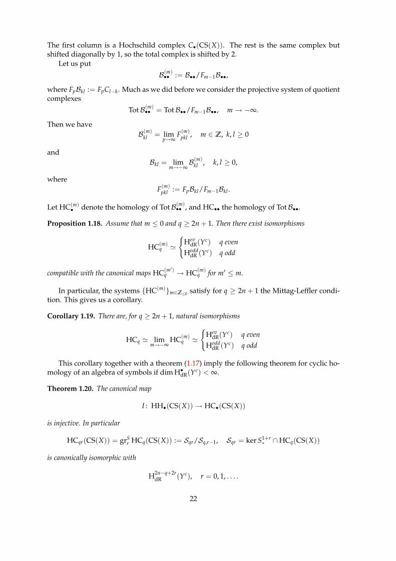
Proposition 1.18. Assume that m ≤ 0 and q ≥ 2n + 1. Then there exist isomorphisms

HC(m)q '

Hev

dR(Yc) q even

HodddR (Yc) q odd

compatible with the canonical maps HC(m′)q → HC

(m)q for m′ ≤ m.

In particular, the systems HC(m)m∈Z≤0satisfy for q ≥ 2n + 1 the Mittag-Leffler condi-

tion. This gives us a corollary.

Corollary 1.19. There are, for q ≥ 2n + 1, natural isomorphisms

HCq ' limm→−∞

HC(m)q '

Hev

dR(Yc) q even

HodddR (Yc) q odd

This corollary together with a theorem (1.17) imply the following theorem for cyclic ho-mology of an algebra of symbols if dim H•

dR(Yc) < ∞.

Theorem 1.20. The canonical map

I : HH•(CS(X)) → HC•(CS(X))

is injective. In particular

HCqr(CS(X)) = grSr HCq(CS(X)) := Sqr/Sq,r−1, Sqr = ker S1+r

∗ ∩ HCq(CS(X))

is canonically isomorphic with

H2n−q+2rdR (Yc), r = 0, 1, . . . .

22

With some more work we can prove the theorem without assumption of finite dimensionof H•

dR(Yc). Then one represents X as a union⋃

j∈N Xj, where each Xj is compact (withsmooth or empty boundary) and Xj ⊂ Int Xj+1. Then the restriction maps CS(X) → CS(Xj)induce homomorphisms

θ : HH•(CS(X)) → HH• := limj

HH•(CS(X)), (1.7)

η : HC•(CS(X)) → HC• := limj

HC•(CS(X)). (1.8)

For each q there is a commutative diagram

HHq(CS(X))θq //

'

²²

HHq

'²²

H2n−qdR

// limj H2n−qdR (Yc

j )

Notice that also the lower arrow is an isomorphism, since

Ω•O = lim

jΩ•

Oj,

where Oj denotes the corresponding graded algebra of functions on Ycj . Since both projective

systems Ω•j and H•

dR(Ycj ) satisfy Mittag-Leffler condition, we have that θ in (1.7) is an

isomorphism.

The naturality of the Connes exact sequence gives us the commutative diagram

. . . 0 // HHqI // HCq

S // HCq−20 // HHq−1

I // . . .

. . . B // HHqI //

'θq

OO

HCqS //

ηq

OO

HCq−2B //

ηq−2

OO

HHq−1I //

'θq−1

OO

. . .

with a priori only the lower sequence being exact. The exactness of the upper sequencefollows from

1

lim HHq(CS(Xj)) = 0, for all q ∈ N,

which is a consequence of the finite-dimensionality of the groups HHq(CS(Xj)) = HdR(Ycj ).

Thus the ”five lemma” and an easy inductive argument prove that η is an isomorphism andB = 0.

Now it remains to prove the proposition (1.18). The filtration F(m)p•• | p = m, m + 1, . . .

on B(m)•• induces a filtration on TotB

(m)•• . Denote by E

(m),rpq the associated spectral sequence

which converges to HC(m)• .

This spectral sequence is a priori located in the region (p, q) | p ≥ m, p + q ≥ 0. We

23

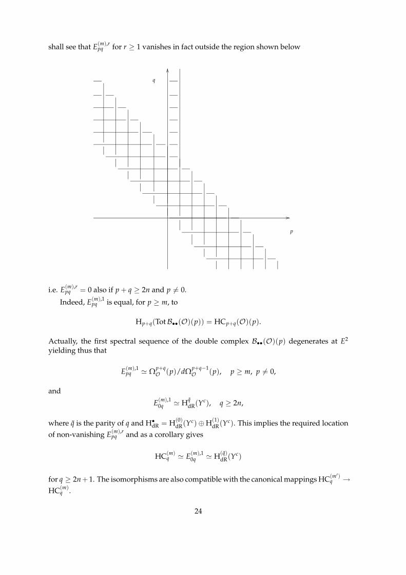
shall see that E(m),rpq for r ≥ 1 vanishes in fact outside the region shown below

q

//

p

OO

i.e. E(m),rpq = 0 also if p + q ≥ 2n and p 6= 0.

Indeed, E(m),1pq is equal, for p ≥ m, to

Hp+q(TotB••(O)(p)) = HCp+q(O)(p).

Actually, the first spectral sequence of the double complex B••(O)(p) degenerates at E2

yielding thus that

E(m),1pq ' Ω

p+qO (p)/dΩ

p+q−1O (p), p ≥ m, p 6= 0,

and

E(m),10q ' H

qdR(Yc), q ≥ 2n,

where q is the parity of q and H•dR = H

(0)dR(Yc) ⊕ H

(1)dR(Yc). This implies the required location

of non-vanishing E(m),rpq and as a corollary gives

HC(m)q ' E

(m),10q ' H

(q)dR(Yc)

for q ≥ 2n + 1. The isomorphisms are also compatible with the canonical mappings HC(m′)q →

HC(m)q .

24

1.9.1 Further analysis of spectral sequence

We will use the notation ′E(m),rpq for the earlier spectral sequence converging to Hochschild

homology HH(m).First, let us consider the morphism of spectral sequences induced by S

′E(m),rpq

S(m),rpq

²²′E

(m),rp,q−2

For r=1 we have

E(m),1pq =

HCp+q(O)(p), O = gr(CS(X)) =

⊕p∈Z O(p) p ≥ m

0 p < m

Then

E(m),1pq

S(m),1pq

²²

E(m),1p,q−2

is the corresponding component of the S-map on cyclic homology of graded algebra O.If p = 0

HCp+q(O) = Ωq⊕ H

q−2dR ⊕H

q−4dR ⊕ . . . ,

whereΩ• := Ω•

O , H•dR := H•(Ω•).

Ωk(p) := Ωk(p)/dΩk−1(p)

For p 6= 0

HCp+q(O)(p) =

Ω

p+q(p) p ≥ m

0 p < m

p = −2 p = −1 p = 0 p = 1 p = 2

Ωq−2

(−2)

0²²

Ωq−1

(−1)

0²²

d1oo Ω

q⊕ H

q−2dR ⊕H

q−4dR ⊕ . . .

²²

d1oo Ω

q+1(1)

²²

d1oo Ω

q+2(2)

²²

d1oo

Ωq−2

(−4) Ωq−1

(−3)d1

oo Ωq−2

⊕ Hq−4dR ⊕H

q−4dR ⊕ . . .

d1oo Ω

q−1(1)

d1oo Ω

q(2)

d1oo

where for p = 0 we have

Ωq

²²

⊕ Hq−2dR²²

²²

⊕ Hq−4dR

⊕ . . .

0 ⊕ Ωq−2 ⊕ H

q−4dR

⊕ . . .

25

Denote

E(m),1pq :=

Ω

p+q(p) p ≥ 0

0 p < 0

Corollary 1.21. There is an isomorphism of chain complexes

(E(m),1•,q , d1

•,q) ' (E(m),1•,q ⊕ (H

q−2dR ⊕H

q−4dR ⊕ . . .)[0], d)

and there is an exact sequence of complexes

0

²²

(Hq−1dR [0], 0)

²²²²

(E(m),1•,q−1, d1)

B²²

(′E(m),1•,q , d1)

²²²²

(E(m),1•,q , d1)

²²0

Consider the second spectral sequence of the double complex but arranged according toconventions of Cartan-Eilenberg’s book. Denote it by qE

r••, although it depends also on m.

The qE2•• looks as follows.

Hq−2dR

E(m),2−2,q−1

ÀÀ ÀÀ::

::

::

::

::

E(m),2−1,q−1

¿¿ ¿¿99

99

99

99

99

E(m),20,q−1

¾¾ ¾¾77

77

77

77

77

E(m),21,q−1

¾¾ ¾¾77

77

77

77

77

E(m),22,q−1

¾¾ ¾¾77

77

77

77

77

E(m),23,q−1

0 0 0 0 0 0

E(m),2−2,q−1 E

(m),2−1,q−1 E

(m),20,q−1 E

(m),21,q−1 E

(m),22,q−1 E

(m),23,q−1

There is an isomorphism

E(m),2pq

'−→ E

(m),2p+1,q+1

except (p, q) = (0, q), (1, q − 1), (1, q), (2, q).

The term E(m),2pq appears twice, in qE

r•• and q+1E

r••.

There are two cases:

q < n then for l =[ q

2

]+ 1

E(m),20

'←− E

(m),2−1,q−1

'←− E

(m),2−2,q−2

'−→ . . .

'−→ E

(m),2−l,q−l ⊆ HCq−2l(O)(−l) = 0

because q − 2l < 0.

26

The E1-term is the same as the E2-term:

Hq−1dR

""FFFFFFFFFFFFFFFFFFFFFFFF

0 0 0 E(m),20,q−1 = 0 E

(m),21,q−1 = 0 E

(m),22,q−1

0 0 0 0 0 0

0 0 0 0 E(m),21,q E

(m),22,q

In E3 there are only two terms and the spectral sequence collapses at E4.

Hq−1dR

½½66

66

66

66

66

66

66

66

66

0 0 0 0 0 Hq−2dR H

q−3dR

0 0 0 0 0 0 0

0 0 0 0 0 Hq−1dR H

q−2dR

q − 1 ≥ n then for l = n −[ q

2

]

E(m),22,q−1

'−→ E

(m),23,q

'−→ E

(m),24,q+1

'−→ . . .

'−→ E

(m),22+l,q+l−1 ' Ω

2l+q−1(2 + l) = 0

because 2l + q − 1 > 2n.

Hn−1dR

0 0 0 0 0 E(m),22,n−1 E

(m),23,n−1

Hn+3dR Hn+2

dR Hn+1dR

HndR Hn−1

dR Hn−2dR Hn−3

dR

0 E(m),2−2,n E

(m),2−1,n E

(m),20,n 0 0 0

27

q

//

OO

p

28

· · · 0 0 0 H2n+2 ⊕H2n+1 0 · · ·

· · · 0 0 0 H2n+1 ⊕H2n 0 · · ·

· · · 0 0 0 H2n ⊕H2n−1 0 · · ·

· · · 0 0 H2n H2n−1 ⊕H2n−3 0 · · ·

· · · 0 H2n H2n−1 H2n−2 ⊕H2n−4 0 · · ·

· · · H2n H2n−1 H2n−2 H2n−3 ⊕H2n−5 0 · · ·

· · · · · · · · · · · · · · · · · · · · · · · · · · · · · · · · · · · · · · · · · · · · · · · · · · · · · · · · · · · · · · ·

n + 2 0 0 0 H2n H2n−1 · · · Hn+5 Hn+4 Hn+3 Hn+2 ⊕Hn 0 0 0 0 0 · · · 0 0 0 0

n + 1 0 0 H2n H2n−1 H2n−2 · · · Hn+3 Hn+3 Hn+2 Hn+1 ⊕Hn−1 0 0 0 0 0 · · · 0 0 0 0

n 0 H2n H2n−1 H2n−2 H2n−3 · · · Hn+3 Hn+2 Hn+1 Hn ⊕Hn−2 0 0 0 0 0 · · · 0 0 0 0

n − 1 0 0 0 0 0 · · · 0 0 0 Hn−3 ⊕Hn−5 0 Hn−2 Hn−3 Hn−4 Hn−5 · · · H3 H2 H1 H0

n − 2 0 0 0 0 0 · · · 0 0 0 Hn−4 ⊕Hn−6 0 Hn−3 Hn−4 Hn−5 Hn−6 · · · H2 H1 H0 0

0 0 0 0 0 · · · 0 0 0 Hn−5 ⊕Hn−7 0 Hn−4 Hn−5 Hn−6 Hn−7 · · · H1 H0 0 0· · · · · · · · · · · · · · · · · · · · · · · · · · · · · · · · · · · · · · · · · · · · · · · · · · · · · · · · · · · · · · ·

· · · 0 0 0 H2 ⊕H0 0 H3 H2 H1 H0 · · ·

· · · 0 0 0 H1 0 H2 H1 H0 0 · · ·

· · · 0 0 0 H0 0 H1 H0 0 0 · · ·

· · · 0 0 0 0 0 H0 0 0 0 · · ·

· · · 0 0 0 0 0 0 0 0 0 · · ·//

. . . −n − 1 −n . . . −4 −3 −2 −1

OO

0 1 2 3 4 . . . n − 1 n . . .

29

1.9.2 Higher differentials

For r = 1, 2, . . . the differentials in the spectral sequence are as follows

•oo

ggNNNNNNNNNN

ddIIIIIIIIIIIIIIIII

ccGGGGGGGGGGGGGGGGGGGGGGG

bbEEEEEEEEEEEEEEEEEEEEEEEEEEEEEE

p//

q

OO

Let Erpq be a spectral sequence such that each Er

pq (for r > r0) is a finite dimensional vectorspace. Let R be a region in the (p, q)-plane which contains finitely many boxes. Then

∑(p,q)∈R

dim Erpq ≥ ∑

(p,q)∈R

dim Er+1pq ≥ . . . ≥ ∑

(p,q)∈R

dim E∞pq.

The equality holds if and only if there is no nontrivial differential originating or leaving R,that is the equality

∑(p,q)∈R

dim Er′

pq = ∑(p,q)∈R

dim E∞pq

is another way of saying that the spectral sequence in region R degenerates at Er′ .In our spectral sequence

E(m),2pq =⇒ Hp+q(TotB••(CS(X))/Fm−1 TotB••(CS(X)))

We claim that the only nonvanishing differentials drpq for r ≥ 2 are

dppq : E

(m),ppq → E

(m),20,p+q−1

which inject E(m),2pq = E

(m),2pq ' H

q−2dR into E

(m),p0,p+q−1.

We can define two regions R, R′ as follows.

[PICTURE]

Then

∑(p,q)∈R

dim Er′

pq = ∑(p,q)∈R

dim E∞pq.

Suppose that ther is no nontrivial differential originating from R′ or nontrivial differentialhitting R and originating outside. Then

∑(p,q)∈R′

dim Erpq − ∑

(p,q)∈R

dim Erpq ≥ ∑

(p,q)∈R′

dim Er+1pq − ∑

(p,q)∈R

dim Er+1pq

30

Equality holds if and only if all dr inside R are zero, and then for all r > r0 for some r0

∑(p,q)∈R′

dim Erpq − ∑

(p,q)∈R

dim Erpq = ∑

(p,q)∈R′

dim E∞pq − ∑

(p,q)∈R

dim E∞pq.

We can write

∑0≤q≤n

dim E(m),20q − ∑

0≤q≤n

dim E(m),∞0q = ∑

p>0

dim E(m),2pq .

For r ≥ 2 let us introduce the following statements:

(A)r The natural maps

E(m),rpq → E

(m),rpq 〈Yn−1〉

are isomorphisms for p > 0, r fixed.

(B)r The differentials

drpq : E

(m),rrq → E

(m),r0,q+r−1

are injective.

(C)r The differentials

drpq : E

(m),rpq → E

(m),rp−r,q+r−1

are zero for p ≥ r.

We prove them by induction on r, simultaneously

(B)2

(A)2

8@xxxxxxxx

xxxxxxxx

Á&FF

FFFF

FF

FFFF

FFFF

(C2)

(B)3

(B)2 ∧ (C)2+3 (A)3

8@xxxxxxxx

xxxxxxxx

Á&FF

FFFF

FF

FFFF

FFFF

(C)3

and so on. Furthermore let us introduce two more sequences of statements:

(D)r For p > mdr

pq = limj

drpq,j.

(E)r For p > m

E(m),rpq = lim

jE

(m),rpq 〈Yj〉.

These are also proved by induction on r in the following way. The (E)r implies (D)r and (E)r

and (D)r together with the condition that E(m),rpq 〈Y j〉, E

(m),r+1pq 〈Y j〉 satisfy Mittag-Leffler

condition, imply (E)r+1.The (A)2 statement follows from the following remark. Suppose Hk

dR(Yc) = 0 for k > nand that dim H•

dR(Yc) < ∞. Then

2n−2

∑j=0

dim E(m),20j − ∑

p>0,q

dim E(m),2pq =

2n−2

∑j=0

dim HCj(CSY).

The maps

HjdR(Yc) → H

jdR((Yk)c)

are isomorphisms for j < k, monomorphism for j = k, zero for j > k + 1.

31

Appendix A

Topological tensor products

Let (E, pαα∈A), (F, qββ∈B) be vector spaces with the sytems of seminorms pαα∈A, qββ∈B

respectively. Define a system of seminorms on E ⊗ F by

(pα ⊗ qβ)(τ) := inf ∑ı∈I

pα(ei)qβ( fi), (A.1)

where infimum is taken over all representations τ = ∑i∈I ei ⊗ fi, in which I is a finite set.

Definition A.1. A locally convex space E ⊗ F with topology induced by the system of seminormspα ⊗ qβ(α,β)∈A×B is calles a projective tensor product and denoted by E ⊗π F. Its completion isdenoted by E⊗π F.

A bilinear map

φ : E × F → E⊗π F, (e, f ) 7→ e ⊗ f ,

is continuous in both variables and has the following universal property.

Fact A.2. For every bilinear jointly continuous mapping f : E× F → W into locally convex space Wthere exists unique continuous linear map Lφ : E⊗π F → W such that following diagram commutes.

E × Ff

//

φ $$IIIIIIIII W

E⊗π F

Lφ

<<xx

xx

Remark A.3. There are also different tensor products on topological vector spaces, like injec-tive and inductive tensor products, but we will not describe them here.

Suppose that E′ =⋃

m∈Z E′m, where

. . . ⊆ E′m−1 ⊆ E′

m ⊆ . . .

is a Z-filtration of E′ by locally convex closed vector subspaces of E′, and analogously forthe space E′′. Then define

E′⊗E′′ := lim(l1,l2)∈Z×Z

E′l1⊗πE′′

l2.

If for any m there is a continuous projections E′m → E′

m−1, E′′m → E′′

m−1, then the spaceE′

l1⊗πE′′

l2is a closed subspace in E′

m1⊗πE′′

m2for any m1 ≥ l1, m2 ≥ l2.

32

Define a Z-filtration on E′⊗E′′

(E′⊗E′′)m :=⋃

(l1,l2)∈Z×Z

l1+l2≤m

E′l1⊗πE′′

l2.

In similar way we define E(1)⊗ . . . ⊗E(p) with Z-filtration

(E(1)⊗ . . . ⊗E(p))m :=⋃

(l1,...,lp)∈Zp

l1+...+lp≤m

E(1)l1

⊗π . . . ⊗πE(p)lp

.

33

Appendix B

Spectral sequences

Lecture given by prof. Wodzicki on October 2004 in Warsaw,with remarks added in November 2006.

B.1 Spectral sequence of a filtered complex

Let (C•, F, ∂) be a filtered chain complex, that is

. . . ⊆ FpC• ⊆ Fp+1C• ⊆ . . . ⊆ C•.

We say that the filtration is

1. separable if⋂

p FpCn = 0,

2. complete if Cn'−→ limp Cn/FpCn,

3. cocomplete if⋃

p FpCn'−→ Cn,

for all n ∈ Z.

We define E0•• := grF

• C• (the associated graded complex), where E0pq := FpCp+q/Fp−1Cp+q,

and d0•• is the boundary operator induced by ∂, d0

pq : E0pq → E0

p,q−1. Thus (E0••, d0

••) is the di-

rect sum of complexes

(E0••, d0

••) =⊕

p∈Z

(E0p•, d0

p•).

Next we define

E1pq := Hq(E0

p•, d0p•)

=c ∈ FpCp+q | ∂c ∈ Fp−1Cp+q−1

c ∈ FpCp+q | c = ∂b for some b ∈ FpCp+q+1mod Fp−1Cp+q

=:Z1

pq + Fp−1Cp+q

B1pq + Fp−1Cp+q

.

On E1pq the boundary operator ∂ induces a boundary operator d1

pq : E1pq → E1

p−1,q and so on...

34

Define for r = 1, 2, . . .

Erpq =

c ∈ FpCp+q | ∂c ∈ Fp−rCp+q−1

c ∈ FpCp+q | c = ∂b for some b ∈ Fp+r−1Cp+q+1mod Fp−1Cp+q

=:Zr

pq + Fp−1Cp+q

Brpq + Fp−1Cp+q

.

. . . Fp−rCp+q−1 Fp−rCp+q Fp−rCp+q+1 . . .

. . . ......

.... . .

. . . Fp−1Cp+q−1 Fp−1Cp+q Fp−1Cp+q+1 . . .

. . . FpCp+q−1 FpCp+q∂0

oo

∂1ggNNNNNNNNNNN

∂r

YY333333333333333333333333333

FpCp+q+1∂0

oo

∂1ggNNNNNNNNNNN

∂r

YY333333333333333333333333333

. . .

. . . Fp+1Cp+q−1 Fp+1Cp+q∂0

oo Fp+1Cp+q+1∂0

oo . . .

. . . ......

.... . .

. . . Fp+rCp+q−1 Fp+rCp+q∂0

oo

∂r

YY333333333333333333333333333

Fp+rCp+q+1∂0

oo

∂r

YY333333333333333333333333333

. . .

. . . ......

.... . .

. . . Cp+q−1 Cp+q∂oo Cp+q+1

∂oo . . .

Now Er•• equipped with the boundary operator induced by ∂ becomes a direct sum of

complexes

. . . ← Erp−r,q+r−1

drpq

←− Erpq

drp+r,q−r+1

←−−−−− Erp+r,q−r+1 ← . . . ,

Erp−r,q+r−1 Er

p−r+1,q+r−1 . . . . . . . . . . . . . . . . . .

. . . . . . . . . Erpq

llXXXXXXXXXXXXXXXXXXXXXXXXXXXXX Erp+1,q

kkWWWWWWWWWWWWWWWWWWWW. . . . . . . . .

. . . . . . . . . . . . . . . . . . Erp+r,q−r+1

kkWWWWWWWWWWWWWWWWWWWWWWW

Erp+r+1,q−r+1

llXXXXXXXXXXXXXXXXXXXXXXXXXX

which we can denote by (Erp+•r,q−•(r−1), dr

p+•r,q−•(r−1)). Now Er+1pq is canonically isomorphic

to the homology of the complex (Erp+•r,q−•(r−1), dr

p+•r,q−•(r−1)) at the Erpq.

35

For each (p, q) we defined a system of subobjects of FpCp+q:

0 = B0pq ⊆ B1

pq ⊆ . . . ⊆ Brpq ⊆ . . .

⊆⋃

r

Brpq =: B∞

pq ⊆ Z∞pq :=

⋂

r

Zrpq ⊆

. . . ⊆ Zrpq ⊆ . . . ⊆ Z1

pq ⊆ Z0pq = FpCp+q,

such thatEr

pq = Zrpq/Br

pq mod Fp−1Cp+q.

Morphism ϕ : (C•, F, ∂) → (′C•,′ F,′ ∂) of filtered complexes induces a morphism

Er••(ϕ) : Er

•• →′ Er

••, r ≥ 0,

of corresponding spectral sequences.

Theorem B.1 (Eilenberg-Moore). If Er••(ϕ) is an isomorphism for some r and both filtrations are

complete and cocomplete, then ϕ is a quasi-isomorphism.

We say that the spectral sequence Er•• converges to filtered module M if

E∞pq ' Fp Mp+q/Fp−1Mp+q, p, q ∈ Z.

We write then Erpq =⇒ Mp+q.

If the filtration is locally bounded from below (i.e. FpCn = 0 for p ¿ 0) and cocom-plete, then Er

•• converges to H∗(C•, ∂). The homology of a complex (C•, ∂) is equipped withcanonical filtration

Fp H∗(C•, ∂) := im(H∗(FpC•, ∂) → H∗(C•, ∂)).

We say that the spectral sequence Er•• degenerates (or collapses) at Es if Es

•• ' E∞••.

Consider the r-th term Er of the spectral sequence.

@@@@

@@

•

ÂÂ???

????

????

????

????

•

@@@@

@@

p//

q

OO

The source term Erpq is mapped to the rightmost one Er

p′q′ . There is a sequence of maps

Erpq ³ Er+1

pq ³ · · · ³ E∞pq → Hp+q(C),

and similarlyHp′+q′(C) → E∞

p′q′ ½ · · · ½ Er+1p′q′ ½ Er

p′q′ .

These maps are called the edge homomorphisms. For the first quadrant spectral sequencethey correspond to maps from leftmost column p = 0

Er0q → Hq(C),

and to bottom row q = 0Hp(C) → Er

p0.

36

B.2 Examples

Example B.2. Two spectral sequences associated with the double complex (C••, ∂′, ∂′′).

...

²²

...

²²

...

²². . . Cp−1,q+1

∂′′

²²

oo Cp,q+1∂′oo

∂′′

²²

Cp+1,q+1∂′oo

∂′′

²²

. . .oo

. . . Cp−1,qoo

∂′′

²²

Cpq∂′oo

∂′′

²²

Cp+1,q∂′oo

∂′′

²²

. . .oo

. . . Cp−1,q−1oo

²²

Cp,q−1∂′oo

²²

Cp+1,q−1∂′oo

²²

. . .oo

......

...

Recall that

∂′2 = ∂′′2 = 0, [∂′, ∂′′] = ∂′∂′′ + ∂′′∂′ = 0,

and the total complex is defined by

(Tot C)n :=−1

∏p=−∞

Cp,n−p ⊕⊕

Cp,n−p, ∂ := ∂′ + ∂′′.

......

.... . . ...

.... . . • • • . . . • • . . .. . . C0,n • • . . . • • . . .

. . . • C1,n−1 • . . . • • . . .

. . . • • C2,n−2 . . . • • . . .

. . . • • • . . . Cn−1,1 • . . .

. . . • • • . . . • Cn0. . .

......

.... . . ...

...

There are two filtrations on Tot C:

1. filtration by columns

′Fp(Tot C)n := ∏r≤p

Cr,n−r

37

......

.... . . ...

p .... . . ...

.... . . • • • . . . • • . . . • • . . .. . . C0,n • • . . . • • . . . • • . . .

. . . • C1,n−1 • . . . • • . . . • • . . .

. . . • • C2,n−2 . . . • • . . . • • . . .

. . . • • • . . . Cp,n−p • . . . • • . . .

. . . • • • . . . • Cp+1,n−p−1 . . . • • . . .

. . . • • • . . . • • . . . Cn−1,1 • . . .

. . . • • • . . . • • . . . • Cn0. . .

......

.... . . ...

p .... . . ...

...

2. filtration by rows′′Fp(Tot C)n :=

⊕

p≤s

Cn−s,s

......

.... . . ...

.... . . ...

.... . . • • • . . . • • . . . • • . . .. . . C0,n • • . . . • • . . . • • . . .

. . . • C1,n−1 • . . . • • . . . • • . . .

. . . • • C2,n−2 . . . • • . . . • • . . .

. . . • • • . . . Cn−p,p • . . . • • . . .

p p

. . . • • • . . . • Cn−p−1,p+1 . . . • • . . .

. . . • • • . . . • • . . . Cn−1,1 • . . .

. . . • • • . . . • • . . . • Cn0. . .

......

.... . . ...

.... . . ...

...

Filtration by rows is complete and cocomplete only if for all n ∈ Z Cpq 6= 0 for only finitenumber of p, q such that p + q = n. Filtration by columns is always complete and cocom-plete.

There are two spectral sequences associated to double complex (C••, ∂′, ∂′′).

1. First spectral sequence associated to the filtration by columns

′E1pq = Hq(Cp•, ∂′′).

It converges to Hp+q(C••) := Hp+q(Tot(C••)) if Cp,n−p = 0 for p ¿ 0 (n ∈ Z).

2. Second spectral sequence associated to the filtration by rows

′′E1pq = Hq(C•p, ∂′).

It converges to Hp+q(C••) if Cp,n−p = 0 for p ¿ 0 and p À 0 (n ∈ Z).

Example B.3. Double complex B(A)•• (Connes double complex). Let A be the associativealgebra with unit.

B(A)pq :=

A⊗(q−p+1) if q ≥ p ≥ 0,

0 otherwise.

38

...

²²

...

²²

...

²²

...

A⊗3

b²²

A⊗2

b²²

Boo ABoo

A⊗2

b²²

ABoo

A

Here b is the Hochschild boundary operator and B is defined as

B := (1 − t)sN,

where

s(a0 ⊗ · · · ⊗ an) := 1 ⊗ a0 ⊗ · · · ⊗ an

t(a0 ⊗ · · · ⊗ an) := (−1)n ⊗ a0 ⊗ · · · ⊗ an−1

N(a0 ⊗ · · · ⊗ an) := (id + t + . . . + tn)(a0 ⊗ · · · ⊗ an)

Example B.4. Double complex D(A)••. Here A is commutative k-algebra with unit.

D(A)pq :=

Ω

q−pA/k if q ≥ p ≥ 0,

0 otherwise.

...

²²

...

²²

...

²²

...

Ω2A/k

0²²

Ω1A/k

0

²²

doo Adoo

Ω1A/k

0

²²

Adoo

A

If A'−→ A ⊗Z Q (i.e. the additive group (A, +) is uniquely divisible), then the formula

µ(a0 ⊗ · · · ⊗ an) :=1

n!a0da0 ∧ · · · ∧ dan

induces a morphism of double complexes µ : B(A)•• → D(A)••.On the level of spectral sequences associated with the filtration by columns we obtain

surjective maps

E1(pq)(µ) : A⊗(q−p+1)³ Ω

q−pA/k.

These maps are isomorphisms if A is a function algebra on the smooth algebraic variety overa perfect field (i.e. of characteristic 0 or such that kp = k if char(k) = p), or iductive limit ofsuch (for example A = C as Q-algebra).

39

The first spectral sequence of a double complex (D(A)••, 0, d) =⊕

q≥0(ΩqA/k

d←− . . .

d←−

A) degenerates at the term E2:

...

²²

...

²²

...

²²

...

Ω2A/k/dΩ1

A/k

0²²

HdR1(A)

0²²

doo HdR0(A)

doo

Ω1A/k/dA

0

²²

HdR0(A)

doo

A

Thus the first spectral sequence of the double complex (B(A)••, b, B) also degenerates at theterm E2, and we get an isomorphism

HCn(A) := Hn(B(A)••) = ΩnA/k/dΩn−1

A/k ⊕ HdRn−2(A) ⊕ HdR

n−4(A) ⊕ . . . .

Example B.5. Let P• be a projective resolution of a right R-module M, and Q• a projectiveresolution of a left R-module N. Consider the double complex P• ⊗R Q•. Then

′E2pq =

Hp(P• ⊗R N) q = 0,

0 q 6= 0

′′E2pq =

Hp(M ⊗R Q•) q = 0,

0 q 6= 0

Both spectral sequences converge to Hp+q(P• ⊗R Q•) =: TorRp+q(M, N), so we get an impor-

tant canonical isomorphisms

Hp(P• ⊗R N) ' TorRp (M, N) ' Hp(M ⊗R Q•).

They express the fact that the bifunctor ⊗R : Mod − R × R − Mod → Ab is balanced.

Example B.6. Two hiperhomology spectral sequences. A Cartan-Eilenberg resolution of acomplex (C•, ∂) is a double complex (P••, ∂′, ∂′′) with augmentation η : P•0 → C• satisfyingthe following conditions:

1. for all p, q the modules Ppq, im ∂′pq, ker ∂′pq, Hp(P•q, ∂′) are projective,

2. the augmented complexes

Pp•

η

²²

im ∂′p•

η

²²

ker ∂′p•

η

²²

Hp(P•q, ∂′)

η

²²Cp im ∂p ker ∂p Hp(C•, ∂)

40

are projective resolutions.

. . . ...

²²

...

²²

...

²²

. . .

. . . Pp−1,qoo

∂′′q²²

Pp,q

∂′poo

∂′′q²²

Pp+1,q

∂′p+1oo

∂′′q²²

. . .oo

. . . Pp−1,q−1oo

²²

Pp,q−1

∂′poo

²²

Pp+1,q−1

∂′p+1oo

²²

. . .oo

. . . ...

²²

...

²²

...

²²

. . .

. . . Pp−1,1oo

∂′′1²²

Pp,1

∂′poo

∂′′1²²

Pp+1,1

∂′p+1oo

∂′′1²²

. . .oo

. . . Pp−1,0oo

η

²²

Pp,0

∂′poo

η

²²

Pp+1,0

∂′p+1oo

η

²²

. . .oo

. . . Cp−1oo Cp∂poo Cp+1

∂p+1oo . . .oo

Such resolution can be obtained from the arbitrary projective resolutions of Hp(C•, ∂) andim ∂p−1 by gluing them.

PHp•

²²

PZp•

oooo_ _ _ _ _

²²ÂÂ

ÂPB

p−1,•oooo_ _ _ _

²²Hp(Cp, ∂) ker ∂poooo im ∂p−1oooo

PBp•

²²

Pp•oooo_ _ _

²²ÂÂ

ÂPZ

p•oooo_ _ _ _

²²im ∂p Cpoooo ker ∂poooo

For an additive functor F the hiperhomology spectral sequences are the first and secondspectral sequences of a double complex (F(P••), F(∂′), F(∂′′))

′E1pq = (LqF)(Cp),

′′E2pq = F(PH

pq),

and

′E2pq = Hp((LqF)(C•)),

′′E2pq = (LpF)(Hq(C•)).

Both spectral sequences converge to

Lp+qF(C•) := Hp+q(F(P••)).

if C• is bounded from below, that is Cn = 0 for n ¿ 0.Assume that Cn = 0 for n < 0, C• is F-acyclic, that is (L0F)(Cn)

'−→ Cn, (LpF)(Cn) = 0 for

p > 0, and that

Hn(C•) =

M n = 0,

0 n > 0.

41

Such complex is called an F-acyclic resolution of the module M. In that case

′E2pq '

Hp(F(C•)) q = 0,

0 q 6= 0,

′′E2pq '

LpF(M) p = 0,

0 p 6= 0.

Thus we obtain an isomorphism

Hp(F(C•)) ' (LpF)(M).

We proved a very important fact, that to compute (LpF)(M) it is enough to use an arbitraryF-acyclic resolution of M.

Example B.7. Flat module is an F-acyclic module for F = (−) ⊗R N, where N is an arbitraryleft R-module. For R = Z flat modules are the torsion free abelian groups. Thus

0 ← Q/Z ← Q ← Z ← 0

is a flat resolution of the group Q/Z (injective cogenerator of a category of abelian groupsAb). From this we obtain

TorZ1 (Q/Z, A) = ker(A → A ⊗Z Q) = Torsion(A).

Example B.8. Consider two composable additive functors

AG−→ B

F−→ C,

where A,B, C are abelian categories. Let M be an object in A, P• its projective resolution. Inthe hiperhomology spectral sequence we put C• = G(P•). Then if G sends projective objectsinto F-acyclic objects

′E2pq = Hp((LqF)(G(P•))) '

Hp((F G)(P•)) = (Lp(F G))(M) q = 0

0 q 6= 0

′′E2pq = (LpF LqG)(M)

In this case we obtain that

′′E2pq = (LpF LqG)(M) =⇒ (Lp+q(F G))(M).

′E2pq = E∞

pq = . . . . . . . . . . . .

0 0 . . . 0

0 0 . . . 0

(L0(F G))(M) (L1(F G))(M) . . . (Lp(F G))(M)

p//

q

OO

42

′′E2pq = . . . . . . . . . . . .

(L0F LqG)(M) (L1F LqG)(M) . . . (LpF LqG)(M)

. . . . . . . . . . . .

(L0F L1G)(M) (L1F L1G)(M) . . . (LpF L1G)(M)

(L0F L0G)(M) (L1F L0G)(M) . . . (LpF L0G)(M)

p//

q

OO

This spectral sequence is called a spectral sequence of a composition of functors.

Example B.9. Let ϕ : R → S be a homomorphism of unital rings, M a right R-module, N aleft S-module. Consider a composition

Mod − RG=(−)⊗RS−−−−−−→ Mod − S

F=(−)⊗R N−−−−−−→ Ab

The spectral sequence of a composition of these two functors (G sends projective R-modulesinto projective S-modules) in looks as follows:

E2pq = TorS

p(TorRq (M, S), N) =⇒ TorR

p+q(M, N)

and it is called a base change spectral sequence.

Suppose that R → S is a homomorphism of k-algebras, MR, SN are respectively right R-module and left S-module. Their tensor product M ⊗ RN gives rise to a sequence of derivedfunctors TorR

• (M, N).

Suppose that P• ³ M is a projective R-module resolution of M, and Q• ³ N a projectiveS-module resolution for N.

M ⊗R N ← P• ⊗R Q• ' (P• ⊗R S) ⊗S Q•

Suppose F(·, ·) is a functor with both covariant arguments.

LqF(·, ·) L1,2q F(·, ·)

wwppppppppppp

''NNNNNNNNNNN

L1q F(·, ·)

''NNNNNNNNNNNL2q F(·, ·)

wwppppppppppp

L∅q F(·, ·)

F if q = 0

0 if q 6= 0

43

We say that it is left balanced if there are isomorphisms L1q ' L

1,2q ' L

2q .

RqF(·, ·) Rq1,2F(·, ·)

Rq1F(·, ·)

77ppppppppppp

Rq2F(·, ·)

ggNNNNNNNNNNN

Rq∅

F(·, ·)

ggOOOOOOOOOOO

77ooooooooooo

F if q = 0

0 if q 6= 0

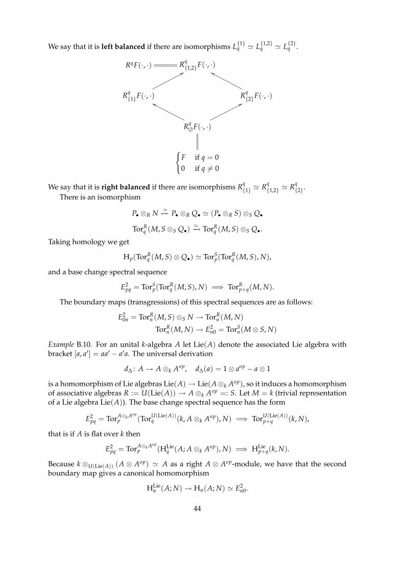
We say that it is right balanced if there are isomorphisms Rq1 ' R

q1,2 ' R

q2.

There is an isomorphism

P• ⊗R N'←− P• ⊗R Q• ' (P• ⊗R S) ⊗S Q•

TorRq (M, S ⊗S Q•)

'−→ TorR

q (M, S) ⊗S Q•.

Taking homology we get

Hp(TorRq (M, S) ⊗ Q•) ' TorS

p(TorRq (M, S), N),

and a base change spectral sequence

E2pq = TorS

p(TorRq (M, S), N) =⇒ TorR

p+q(M, N).

The boundary maps (transgressions) of this spectral sequences are as follows:

E20n = TorR

n (M, S) ⊗S N → TorRn (M, N)

TorRn (M, N) → E2

n0 = TorSn(M ⊗ S, N)

Example B.10. For an unital k-algebra A let Lie(A) denote the associated Lie algebra withbracket [a, a′] = aa′ − a′a. The universal derivation

d∆ : A → A ⊗k Aop, d∆(a) = 1 ⊗ aop − a ⊗ 1

is a homomorphism of Lie algebras Lie(A) → Lie(A⊗k Aop), so it induces a homomorphismof associative algebras R := U(Lie(A)) → A ⊗k Aop =: S. Let M = k (trivial representationof a Lie algebra Lie(A)). The base change spectral sequence has the form

E2pq = TorA⊗k Aop

p (TorU(Lie(A))q (k, A ⊗k Aop), N) =⇒ Tor

U(Lie(A))p+q (k, N),

that is if A is flat over k then

E2pq = TorA⊗k Aop

p (HLieq (A; A ⊗k Aop), N) =⇒ HLie

p+q(k, N).

Because k ⊗U(Lie(A)) (A ⊗ Aop) ' A as a right A ⊗ Aop-module, we have that the secondboundary map gives a canonical homomorphism

HLien (A; N) → Hn(A; N) ' E2

n0.

44

There is a homomorphism of standard chain complexes

(C•(Lie(A); N), ∂) → (C•(A, N), b)

where

∂(n ⊗ a1 ∧ · · · ∧ an) :=n

∑i=1

(−1)i (ain − nai)︸ ︷︷ ︸−(d∆a)n

⊗a1 ∧ · · · ∧ ai ∧ · · · ∧ an

+ ∑1≤i<j≤n

(−1)i+jn ⊗ [ai, aj] ∧ a1 ∧ · · · ∧ ai ∧ · · · ∧ aj ∧ · · · ∧ an

In the special case N = A we obtain canonical homomorphism

HLien (A; ad) → HHn(A)

Example B.11. Hiper-Tor spectral sequences and Kunneth spectral sequence. For a right R-module M and a complex of left modules C• we define

TorRn (M, C•) := Hn(P• ⊗R C•)

where P• → M is a projective resolution of M. Then the first and second spectral sequenceof a bicomplex P• ⊗R C• are as follows:

′E1pq = Pp ⊗R Hq(C)

′E2pq = TorR

p (M, Hq(C)) =⇒ TorRp+q(M, C•)

and

′′E1pq = TorR

q (M, Cp)

′′E2pq = Hp(TorR

q (M, C•)) '

Hp(M ⊗R C•) q = 0

0 q 6= 0

where the isomorphism for E2pq holds if the complexes TorR

q (M, C•) are acyclic for q > 0, forexample if Cn are flat. Then we obtain a Kunneth spectral sequence

E2pq = TorR

p (M, Hq(C)) =⇒ Hp+q(M ⊗R C•)

if Cn = 0 for n ¿ 0.

Example B.12. If a group G acts on semigroup S and its representation V, then G acts onBar-complex (B•(S; V), b′), where Bq(S; V) = (kS)⊗kq ⊗k V, and b′ is a standard boundaryoperator. Then

Tork[G]n (G, B•(S; V)) =: HG

n (S; V)

are the equivariant homology of a semigroup S with coefficients in representation V. In ananalogous way one can define equivariant homology of a Lie algebra, Hochschild homology,singular homology of a topological space etc.

45