LECTURES ON GRAVITATIONAL LENSING

RAMESH NARAYAN1 AND MATTHIAS BARTELMANN2

1HARVARD-SMITHSONIAN CENTER FOR ASTROPHYSICS, 60 GARDEN STREET, CAMBRIDGE, MA 02138, USA2MAX-PLANCK-INSTITUT FUR ASTROPHYSIK, P.O. BOX 1523, D–85740 GARCHING, GERMANY

in: Formation of Structure in the UniverseProceedings of the 1995 Jerusalem Winter School; edited by A. Dekel and J.P. Ostriker; Cambridge University Press

ABSTRACTThese lectures give an introduction to Gravitational Lensing. We discuss lensing by point masses, lensing by

galaxies, and lensing by clusters and larger-scale structures in the Universe. The relevant theory is developed andapplications to astrophysical problems are discussed.

CONTENTS

1. Introduction 1

2. Lensing by Point Masses in the Universe 32.1. Basics of Gravitational Lensing . . . . . . . . . 32.2. Microlensing in the Galaxy . . . . . . . . . . . 72.3. Extragalactic Microlenses . . . . . . . . . . . . 10

3. Lensing by Galaxies 113.1. Lensing by a Singular Isothermal Sphere . . . . 113.2. Effective Lensing Potential . . . . . . . . . . . 123.3. Gravitational Lensing via Fermat’s Principle . . 133.4. Circularly Symmetric Lens Models . . . . . . . 153.5. Non-Circularly-Symmetric Lens Models . . . . 153.6. Studies of Galaxy Lensing . . . . . . . . . . . 173.7. Astrophysical Results from Galaxy Lensing . . 19

4. Lensing by Galaxy Clusters and Large-Scale Struc-ture 214.1. Strong Lensing by Clusters — Giant Arcs . . . 224.2. Weak Lensing by Clusters — Arclets . . . . . . 254.3. Weak Lensing by Large-Scale Structure . . . . 28

1. INTRODUCTION

One of the consequences of Einstein’s General Theory of Rel-ativity is that light rays are deflected by gravity. Although thisdiscovery was made only in this century, the possibility that therecould be such a deflection had been suspected much earlier, byNewton and Laplace among others. Soldner (1804) calculatedthe magnitude of the deflection due to the Sun, assuming thatlight consists of material particles and using Newtonian grav-ity. Later, Einstein (1911) employed the equivalence principle tocalculate the deflection angle and re-derived Soldner’s formula.Later yet, Einstein (1915) applied the full field equations of Gen-eral Relativity and discovered that the deflection angle is actu-ally twice his previous result, the factor of two arising becauseof the curvature of the metric. According to this formula, a lightray which tangentially grazes the surface of the Sun is deflectedby 1:007. Einstein’s final result was confirmed in 1919 when theapparent angular shift of stars close to the limb of the Sun (seeFig. 1) was measured during a total solar eclipse (Dyson, Edding-ton, & Davidson 1920). The quantitative agreement between themeasured shift and Einstein’s prediction was immediately per-ceived as compelling evidence in support of the theory of Gen-eral Relativity. The deflection of light by massive bodies, and the

phenomena resulting therefrom, are now referred to as Gravita-tional Lensing.

FIG. 1.—Angular deflection of a ray of light passing close to the limbof the Sun. Since the light ray is bent toward the Sun, the apparent po-sitions of stars move away from the Sun.

Eddington (1920) noted that under certain conditions theremay be multiple light paths connecting a source and an observer.This implies that gravitational lensing can give rise to multipleimages of a single source. Chwolson (1924) considered the cre-ation of fictitious double stars by gravitational lensing of stars bystars, but did not comment on whether the phenomenon could ac-tually be observed. Einstein (1936) discussed the same problemand concluded that there is little chance of observing lensing phe-nomena caused by stellar-mass lenses. His reason was that theangular image splitting caused by a stellar-mass lens is too smallto be resolved by an optical telescope.

Zwicky (1937a) elevated gravitational lensing from a curiosityto a field with great potential when he pointed out that galaxiescan split images of background sources by a large enough angleto be observed. At that time, galaxies were commonly believedto have masses of 109 M. However, Zwicky had applied thevirial theorem to the Virgo and Coma clusters of galaxies and hadderived galaxy masses of 41011 M. Zwicky argued that thedeflection of light by galaxies would not only furnish an addi-tional test of General Relativity, but would also magnify distantgalaxies which would otherwise remain undetected, and wouldallow accurate determination of galaxy masses. Zwicky (1937b)even calculated the probability of lensing by galaxies and con-cluded that it is on the order of one per cent for a source at rea-sonably large redshift.

Virtually all of Zwicky’s predictions have come true. Lens-ing by galaxies is a major sub-discipline of gravitational lens-ing today. The most accurate mass determinations of the cen-tral regions of galaxies are due to gravitational lensing, and thecosmic telescope effect of gravitational lenses has enabled us to

1

study faint and distant galaxies which happen to be strongly mag-nified by galaxy clusters. The statistics of gravitational lensingevents, whose order of magnitude Zwicky correctly estimated,offers one of the promising ways of inferring cosmological pa-rameters.

In a stimulating paper, Refsdal (1964) described how the Hub-ble constant H0 could in principle be measured through gravita-tional lensing of a variable source. Since the light travel times forthe various images are unequal, intrinsic variations of the sourcewould be observed at different times in the images. The time de-lay between images is proportional to the difference in the ab-solute lengths of the light paths, which in turn is proportionalto H1

0 . Thus, if the time delay is measured and if an accuratemodel of a lensed source is developed, the Hubble constant couldbe measured.

All of these ideas on gravitational lensing remained mere spec-ulation until real examples of gravitational lensing were finallydiscovered. The stage for this was set by the discovery of quasars(Schmidt 1963) which revealed a class of sources that is idealfor studying the effects of gravitational lensing. Quasars are dis-tant, and so the probability that they are lensed by interveninggalaxies is sufficiently large. Yet, they are bright enough to bedetected even at cosmological distances. Moreover, their opticalemission region is very compact, much smaller than the typicalscales of galaxy lenses. The resulting magnifications can there-fore be very large, and multiple image components are well sep-arated and easily detected.

Walsh, Carswell, & Weymann (1979) discovered the first ex-ample of gravitational lensing, the quasar QSO 0957+561A,B.This source consists of two images, A and B, separated by 600.Evidence that 0957+561A,B does indeed correspond to twinlensed images of a single QSO is provided by (i) the similarityof the spectra of the two images, (ii) the fact that the flux ra-tio between the images is similar in the optical and radio wave-bands, (iii) the presence of a foreground galaxy between the im-ages, and (iv) VLBI observations which show detailed corre-spondence between various knots of emission in the two radioimages. Over a dozen convincing examples of multiple-imagedquasars are known today (Keeton & Kochanek 1996) and the listcontinues to grow.

Paczynski (1986b) revived the idea of lensing of stars by starswhen he showed that at any given time one in a million stars inthe Large Magellanic Cloud (LMC) might be measurably mag-nified by the gravitational lens effect of an intervening star inthe halo of our Galaxy. The magnification events, which arecalled microlensing events, have time scales between two hoursand two years for lens masses between 106 M and 102 M.Initially, it was believed that the proposed experiment of mon-itoring the light curves of a million stars would never be fea-sible, especially since the light curves have to be sampled fre-quently and need to be distinguished from light curves of intrin-sically variable stars. Nevertheless, techniques have advancedso rapidly that today four separate collaborations have success-fully detected microlensing events (Alcock et al. 1993; Aubourget al. 1993; Udalski et al. 1993; Alard 1995), and this field hasdeveloped into an exciting method for studying the nature anddistribution of mass in our Galaxy.

Einstein rings, a particularly interesting manifestation of grav-itational lensing, were discovered first in the radio waveband byHewitt et al. (1987). About half a dozen radio rings are nowknown and these sources permit the most detailed modeling yetof the mass distributions of lensing galaxies.

Gravitational lensing by galaxy clusters had been consideredtheoretically even before the discovery of QSO 0957+561. Thesubject entered the observational realm with the discovery of gi-ant blue luminous arcs in the galaxy clusters A 370 and Cl 2244

(Soucail et al. 1987a,b; Lynds & Petrosian 1986). Paczynski(1987) proposed that the arcs are the images of backgroundgalaxies which are strongly distorted and elongated by the grav-itational lens effect of the foreground cluster. This explanationwas confirmed when the first arc redshifts were measured andfound to be significantly greater than that of the clusters.

Apart from the spectacular giant luminous arcs, which re-quire special alignment between the cluster and the backgroundsource, clusters also coherently distort the images of other faintbackground galaxies (Tyson 1988). These distortions are mostlyweak, and the corresponding images are referred to as arclets(Fort et al. 1988; Tyson, Valdes, & Wenk 1990). Observa-tions of arclets can be used to reconstruct parameter-free, two-dimensional mass maps of the lensing cluster (Kaiser & Squires1993). This technique has attracted a great deal of interest,and two-dimensional maps have been obtained of several galaxyclusters (Bonnet et al. 1993; Bonnet, Mellier, & Fort 1994;Fahlman et al. 1994; Broadhurst 1995; Smail et al. 1995; Tyson& Fischer 1995; Squires et al. 1996; Seitz et al. 1996).

As this brief summary indicates, gravitational lensing mani-fests itself through a very broad and interesting range of phenom-ena. At the same time, lensing has developed into a powerful toolto study a host of important questions in astrophysics. The appli-cations of gravitational lensing may be broadly classified underthree categories:

– The magnification effect enables us to observe objectswhich are too distant or intrinsically too faint to be ob-served without lensing. Lenses therefore act as “cosmictelescopes” and allow us to infer source properties far be-low the resolution limit or sensitivity limit of current obser-vations. However, since we do not have the ability to pointthis telescope at any particular object of interest but have towork with whatever nature gives us, the results have beenonly modestly interesting.

– Gravitational lensing depends solely on the projected, two-dimensional mass distribution of the lens, and is indepen-dent of the luminosity or composition of the lens. Lensingtherefore offers an ideal way to detect and study dark matter,and to explore the growth and structure of mass condensa-tions in the universe.

– Many properties of individual lens systems or samples oflensed objects depend on the age, the scale, and the overallgeometry of the universe. The Hubble constant, the cosmo-logical constant, and the density parameter of the universecan be significantly constrained through lensing.

The article is divided into three main sections. Sect. 2. dis-cusses the effects of point-mass lenses, Sect. 3. considers galaxy-scale lenses, and Sect. 4. discusses lensing by galaxy clusters andlarge-scale structure in the universe. References to the originalliterature are given throughout the text. The following are somegeneral or specialized review articles and monographs:

Monograph

– Schneider, P., Ehlers, J., & Falco, E.E. 1992, GravitationalLenses (Berlin: Springer Verlag)

General Reviews

– Blandford, R.D., & Narayan, R. 1992, Cosmological Appli-cations of Gravitational Lensing, Ann. Rev. Astr. Ap., 30,311

– Refsdal, S., & Surdej, J. 1994, Gravitational Lenses, Rep.Progr. Phys., 57, 117

2

– Schneider, P. 1996, Cosmological Applications of Gravi-tational Lensing, in: The universe at high-z, large-scalestructure and the cosmic microwave background, LectureNotes in Physics, eds. E. Martınez-Gonzalez & J.L. Sanz(Berlin: Springer Verlag)

– Wu, X.-P. 1996, Gravitational Lensing in the Universe,Fundamentals of Cosmic Physics, 17, 1

Special Reviews

– Fort, B., & Mellier, Y. 1994, Arc(let)s in Clusters of Galax-ies, Astr. Ap. Rev., 5, 239

– Bartelmann, M., & Narayan, R. 1995, Gravitational Lens-ing and the Mass Distribution of Clusters, in: Dark Matter,AIP Conf. Proc. 336, eds. S.S. Holt & C.L. Bennett (NewYork: AIP Press)

– Keeton II, C.R. & Kochanek, C.S. 1996, Summary of Dataon Secure Multiply-Imaged Systems, in: Cosmological Ap-plications of Gravitational Lensing, IAU Symp. 173, eds.C.S. Kochanek & J.N. Hewitt

– Paczynski, B. 1996, Gravitational Microlensing in the Lo-cal Group, Ann. Rev. Astr. Ap., 34, 419

– Roulet, E., & Mollerach, S. 1997, Microlensing, PhysicsReports, 279, 67

2. LENSING BY POINT MASSES IN THE UNIVERSE

2.1. Basics of Gravitational Lensing

The propagation of light in arbitrary curved spacetimes is in gen-eral a complicated theoretical problem. However, for almost allcases of relevance to gravitational lensing, we can assume thatthe overall geometry of the universe is well described by theFriedmann-Lemaıtre-Robertson-Walker metric and that the mat-ter inhomogeneities which cause the lensing are no more than lo-cal perturbations. Light paths propagating from the source pastthe lens to the observer can then be broken up into three dis-tinct zones. In the first zone, light travels from the source to apoint close to the lens through unperturbed spacetime. In thesecond zone, near the lens, light is deflected. Finally, in thethird zone, light again travels through unperturbed spacetime. Tostudy light deflection close to the lens, we can assume a locallyflat, Minkowskian spacetime which is weakly perturbed by theNewtonian gravitational potential of the mass distribution con-stituting the lens. This approach is legitimate if the Newtonianpotential Φ is small, jΦj c2, and if the peculiar velocity v ofthe lens is small, v c.

These conditions are satisfied in virtually all cases of astro-physical interest. Consider for instance a galaxy cluster at red-shift 0:3 which deflects light from a source at redshift 1.The distances from the source to the lens and from the lens to theobserver are 1 Gpc, or about three orders of magnitude largerthan the diameter of the cluster. Thus zone 2 is limited to a smalllocal segment of the total light path. The relative peculiar veloci-ties in a galaxy cluster are 103 km s1 c, and the Newtonianpotential is jΦj< 104 c2 c2, in agreement with the conditionsstated above.

2.1.1. Effective Refractive Index of a Gravitational Field

In view of the simplifications just discussed, we can describelight propagation close to gravitational lenses in a locallyMinkowskian spacetime perturbed by the gravitational potential

of the lens to first post-Newtonian order. The effect of spacetimecurvature on the light paths can then be expressed in terms of aneffective index of refraction n, which is given by (e.g. Schneideret al. 1992)

n = 1 2c2 Φ = 1+

2c2 jΦj : (1)

Note that the Newtonian potential is negative if it is defined suchthat it approaches zero at infinity. As in normal geometrical op-tics, a refractive index n> 1 implies that light travels slower thanin free vacuum. Thus, the effective speed of a ray of light in agravitational field is

v =cn' c 2

cjΦj : (2)

Figure 2 shows the deflection of light by a glass prism. Thespeed of light is reduced inside the prism. This reduction ofspeed causes a delay in the arrival time of a signal through theprism relative to another signal traveling at speed c. In addition,it causes wavefronts to tilt as light propagates from one mediumto another, leading to a bending of the light ray around the thickend of the prism.

FIG. 2.—Light deflection by a prism. The refractive index n > 1 of theglass in the prism reduces the effective speed of light to c=n. This causeslight rays to be bent around the thick end of the prism, as indicated.The dashed lines are wavefronts. Although the geometrical distance be-tween the wavefronts along the two rays is different, the travel time isthe same because the ray on the left travels through a larger thickness ofglass.

The same effects are seen in gravitational lensing. Because theeffective speed of light is reduced in a gravitational field, lightrays are delayed relative to propagation in vacuum. The totaltime delay ∆t is obtained by integrating over the light path fromthe observer to the source:

∆t =Z observer

source

2c3 jΦjdl : (3)

This is called the Shapiro delay (Shapiro 1964).

3

As in the case of the prism, light rays are deflected when theypass through a gravitational field. The deflection is the integralalong the light path of the gradient of n perpendicular to the lightpath, i.e.

~α =Z~∇?ndl =

2c2

Z~∇?Φdl : (4)

In all cases of interest the deflection angle is very small. We cantherefore simplify the computation of the deflection angle con-siderably if we integrate ~∇?n not along the deflected ray, butalong an unperturbed light ray with the same impact parame-ter. (As an aside we note that while the procedure is straightfor-ward with a single lens, some care is needed in the case of mul-tiple lenses at different distances from the source. With multiplelenses, one takes the unperturbed ray from the source as the ref-erence trajectory for calculating the deflection by the first lens,the deflected ray from the first lens as the reference unperturbedray for calculating the deflection by the second lens, and so on.)

FIG. 3.—Light deflection by a point mass. The unperturbed ray passesthe mass at impact parameter b and is deflected by the angle α. Most ofthe deflection occurs within ∆zb of the point of closest approach.

As an example, we now evaluate the deflection angle of a pointmass M (cf. Fig. 3). The Newtonian potential of the lens is

Φ(b;z) = GM

(b2 + z2)1=2; (5)

where b is the impact parameter of the unperturbed light ray, andz indicates distance along the unperturbed light ray from the pointof closest approach. We therefore have

~∇?Φ(b;z) =GM~b

(b2 + z2)3=2; (6)

where~b is orthogonal to the unperturbed ray and points towardthe point mass. Equation (6) then yields the deflection angle

α =2c2

Z~∇?Φdz =

4GMc2b

: (7)

Note that the Schwarzschild radius of a point mass is

RS =2GM

c2 ; (8)

so that the deflection angle is simply twice the inverse of the im-pact parameter in units of the Schwarzschild radius. As an exam-ple, the Schwarzschild radius of the Sun is 2:95 km, and the solarradius is 6:96105 km. A light ray grazing the limb of the Sun istherefore deflected by an angle (5:9=7:0)105radians = 1:007.

2.1.2. Thin Screen Approximation

Figure 3 illustrates that most of the light deflection occurs within∆z b of the point of closest encounter between the lightray and the point mass. This ∆z is typically much smaller thanthe distances between observer and lens and between lens andsource. The lens can therefore be considered thin compared tothe total extent of the light path. The mass distribution of the lenscan then be projected along the line-of-sight and be replaced by amass sheet orthogonal to the line-of-sight. The plane of the masssheet is commonly called the lens plane. The mass sheet is char-acterized by its surface mass density

Σ(~ξ) =Z

ρ(~ξ;z)dz ; (9)

where~ξ is a two-dimensional vector in the lens plane. The de-flection angle at position~ξ is the sum of the deflections due to allthe mass elements in the plane:

~α(~ξ) =4Gc2

Z(~ξ~ξ0)Σ(~ξ0)j~ξ~ξ0j2

d2ξ0 : (10)

Figure 4 illustrates the situation.

FIG. 4.—A light ray which intersects the lens plane at~ξ is deflected byan angle ~α(~ξ).

4

In general, the deflection angle is a two-component vector. Inthe special case of a circularly symmetric lens, we can shift thecoordinate origin to the center of symmetry and reduce light de-flection to a one-dimensional problem. The deflection angle thenpoints toward the center of symmetry, and its modulus is

α(ξ) =4GM(ξ)

c2ξ; (11)

where ξ is the distance from the lens center and M(ξ) is the massenclosed within radius ξ,

M(ξ) = 2πZ ξ

0Σ(ξ0)ξ0 dξ0 : (12)

2.1.3. Lensing Geometry and Lens Equation

The geometry of a typical gravitational lens system is shown inFig. 5. A light ray from a source S is deflected by the angle ~α atthe lens and reaches an observer O. The angle between the (arbi-trarily chosen) optic axis and the true source position is~β, and theangle between the optic axis and the image I is~θ. The (angulardiameter) distances between observer and lens, lens and source,and observer and source are Dd, Dds, and Ds, respectively.

FIG. 5.—Illustration of a gravitational lens system. The light ray prop-agates from the source S at transverse distance η from the optic axis tothe observer O, passing the lens at transverse distance ξ. It is deflectedby an angle α. The angular separations of the source and the image fromthe optic axis as seen by the observer are β and θ, respectively. The re-duced deflection angle α and the actual deflection angle α are relatedby eq. (13). The distances between the observer and the source, the ob-server and the lens, and the lens and the source are Ds, Dd, and Dds,respectively.

It is now convenient to introduce the reduced deflection angle

~α =Dds

Ds

~α : (13)

From Fig. 5 we see that θDs = βDs + αDds. Therefore, the posi-tions of the source and the image are related through the simpleequation

~β =~θ~α(~θ) : (14)

Equation (14) is called the lens equation, or ray-tracing equa-tion. It is nonlinear in the general case, and so it is possible tohave multiple images~θ corresponding to a single source position~β. As Fig. 5 shows, the lens equation is trivial to derive and re-quires merely that the following Euclidean relation should existbetween the angle enclosed by two lines and their separation,

separation = angledistance : (15)

It is not obvious that the same relation should also hold in curvedspacetimes. However, if the distances Dd;s;ds are defined suchthat eq. (15) holds, then the lens equation must obviously be true.Distances so defined are called angular-diameter distances, andeqs. (13), (14) are valid only when these distances are used. Notethat in general Dds 6= DsDd.

As an instructive special case consider a lens with a constantsurface-mass density. From eq. (11), the (reduced) deflection an-gle is

α(θ) =Dds

Ds

4Gc2ξ

(Σπξ2) =4πGΣ

c2

DdDds

Dsθ ; (16)

where we have set ξ = Ddθ. In this case, the lens equation islinear; that is, β ∝ θ. Let us define a critical surface-mass density

Σcr =c2

4πGDs

DdDds= 0:35gcm2

D

1Gpc

1

; (17)

where the effective distance D is defined as the combination ofdistances

D =DdDds

Ds: (18)

For a lens with a constant surface mass density Σcr, the deflectionangle is α(θ) = θ, and so β = 0 for all θ. Such a lens focuses per-fectly, with a well-defined focal length. A typical gravitationallens, however, behaves quite differently. Light rays which passthe lens at different impact parameters cross the optic axis at dif-ferent distances behind the lens. Considered as an optical device,a gravitational lens therefore has almost all aberrations one canthink of. However, it does not have any chromatic aberration be-cause the geometry of light paths is independent of wavelength.

A lens which has Σ > Σcr somewhere within it is referred toas being supercritical. Usually, multiple imaging occurs only ifthe lens is supercritical, but there are exceptions to this rule (e.g.,Subramanian & Cowling 1986).

2.1.4. Einstein Radius

Consider now a circularly symmetric lens with an arbitrary massprofile. According to eqs. (11) and (13), the lens equation reads

β(θ) = θ Dds

DdDs

4GM(θ)c2 θ

: (19)

Due to the rotational symmetry of the lens system, a sourcewhich lies exactly on the optic axis (β = 0) is imaged as a ring ifthe lens is supercritical. Setting β = 0 in eq. (19) we obtain theradius of the ring to be

θE =

4GM(θE)

c2

Dds

DdDs

1=2

: (20)

5

This is referred to as the Einstein radius. Figure 6 illustrates thesituation. Note that the Einstein radius is not just a property ofthe lens, but depends also on the various distances in the prob-lem.

FIG. 6.—A source S on the optic axis of a circularly symmetric lens isimaged as a ring with an angular radius given by the Einstein radius θE.

The Einstein radius provides a natural angular scale to de-scribe the lensing geometry for several reasons. In the case ofmultiple imaging, the typical angular separation of images is oforder 2θE. Further, sources which are closer than about θE tothe optic axis experience strong lensing in the sense that they aresignificantly magnified, whereas sources which are located welloutside the Einstein ring are magnified very little. In many lensmodels, the Einstein ring also represents roughly the boundarybetween source positions that are multiply-imaged and those thatare only singly-imaged. Finally, by comparing eqs. (17) and (20)we see that the mean surface mass density inside the Einstein ra-dius is just the critical density Σcr.

For a point mass M, the Einstein radius is given by

θE =

4GM

c2

Dds

DdDs

1=2

: (21)

To give two illustrative examples, we consider lensing by a starin the Galaxy, for which M M and D 10 kpc, and lensingby a galaxy at a cosmological distance with M 1011 M andD 1 Gpc. The corresponding Einstein radii are

θE = (0:9mas)

M

M

1=2 D10kpc

1=2

;

θE = (0:009)

M

1011 M

1=2 DGpc

1=2

:

(22)

2.1.5. Imaging by a Point Mass Lens

For a point mass lens, we can use the Einstein radius (20) torewrite the lens equation in the form

β = θ θ2E

θ: (23)

This equation has two solutions,

θ =12

β

qβ2 +4θ2

E

: (24)

Any source is imaged twice by a point mass lens. The twoimages are on either side of the source, with one image insidethe Einstein ring and the other outside. As the source movesaway from the lens (i.e. as β increases), one of the images ap-proaches the lens and becomes very faint, while the other imageapproaches closer and closer to the true position of the source andtends toward a magnification of unity.

FIG. 7.—Relative locations of the source S and images I+, I

lensedby a point mass M. The dashed circle is the Einstein ring with radiusθE. One image is inside the Einstein ring and the other outside.

Gravitational light deflection preserves surface brightness (be-cause of Liouville’s theorem), but gravitational lensing changesthe apparent solid angle of a source. The total flux received froma gravitationally lensed image of a source is therefore changed inproportion to the ratio between the solid angles of the image andthe source,

magnification =image areasource area

: (25)

Figure 8 shows the magnified images of a source lensed by apoint mass.

For a circularly symmetric lens, the magnification factor µ isgiven by

µ =θβ

dθdβ

: (26)

6

FIG. 8.—Magnified images of a source lensed by a point mass.

For a point mass lens, which is a special case of a circularly sym-metric lens, we can substitute for β using the lens equation (23)to obtain the magnifications of the two images,

µ =

"1

θE

θ

4#1

=u2 +2

2up

u2 +4 1

2; (27)

where u is the angular separation of the source from the pointmass in units of the Einstein angle, u = βθ1

E . Since θ < θE,µ < 0, and hence the magnification of the image which is in-side the Einstein ring is negative. This means that this image hasits parity flipped with respect to the source. The net magnifica-tion of flux in the two images is obtained by adding the absolutemagnifications,

µ = jµ+j+ jµj=u2 +2

up

u2 +4: (28)

When the source lies on the Einstein radius, we have β = θE, u =

1, and the total magnification becomes

µ = 1:17+0:17= 1:34 : (29)

How can lensing by a point mass be detected? Unless the lensis massive (M> 106 M for a cosmologically distant source), theangular separation of the two images is too small to be resolved.However, even when it is not possible to see the multiple images,the magnification can still be detected if the lens and source moverelative to each other, giving rise to lensing-induced time vari-ability of the source (Chang & Refsdal 1979; Gott 1981). Whenthis kind of variability is induced by stellar mass lenses it is re-ferred to as microlensing. Microlensing was first observed in themultiply-imaged QSO 2237+0305 (Irwin et al. 1989), and mayalso have been seen in QSO 0957+561 (Schild & Smith 1991;see also Sect. 3.7.4.). Paczynski (1986b) had the brilliant idea ofusing microlensing to search for so-called Massive AstrophysicalCompact Halo Objects (MACHOs, Griest 1991) in the Galaxy.We discuss this topic in some depth in Sect. 2.2..

2.2. Microlensing in the Galaxy

2.2.1. Basic Relations

If the closest approach between a point mass lens and a source is θE, the peak magnification in the lensing-induced light curveis µmax 1:34. A magnification of 1:34 corresponds to a bright-ening by 0:32 magnitudes, which is easily detectable. Paczynski(1986b) proposed monitoring millions of stars in the LMC tolook for such magnifications in a small fraction of the sources.If enough events are detected, it should be possible to map thedistribution of stellar-mass objects in our Galaxy.

Perhaps the biggest problem with Paczynski’s proposal is thatmonitoring a million stars or more primarily leads to the detec-tion of a huge number of variable stars. The intrinsically variablesources must somehow be distinguished from stars whose vari-ability is caused by microlensing. Fortunately, the light curves oflensed stars have certain tell-tale signatures — the light curvesare expected to be symmetric in time and the magnification isexpected to be achromatic because light deflection does not de-pend on wavelength (but see the more detailed discussion in Sect.2.2.4. below). In contrast, intrinsically variable stars typicallyhave asymmetric light curves and do change their colors.

The expected time scale for microlensing-induced variationsis given in terms of the typical angular scale θE, the relative ve-locity v between source and lens, and the distance to the lens:

t0 =DdθE

v= 0:214yr

M

M

1=2 Dd

10kpc

1=2

Dds

Ds

1=2200kms1

v

: (30)

The ratio DdsD1s is close to unity if the lenses are located in the

Galactic halo and the sources are in the LMC. If light curves aresampled with time intervals between about an hour and a year,MACHOs in the mass range 106 M to 102 M are potentiallydetectable. Note that the measurement of t0 in a given microlens-ing event does not directly give M, but only a combination of M,Dd, Ds, and v. Various ideas to break this degeneracy have beendiscussed. Figure 9 shows microlensing-induced light curves forsix different minimum separations ∆y= umin between the sourceand the lens. The widths of the peaks are t0, and there is a di-rect one-to-one mapping between ∆y and the maximum magnifi-cation at the peak of the light curve. A microlensing light curvetherefore gives two observables, t0 and ∆y.

The chance of seeing a microlensing event is usually ex-pressed in terms of the optical depth, which is the probability thatat any instant of time a given star is within an angle θE of a lens.The optical depth is the integral over the number density n(Dd) oflenses times the area enclosed by the Einstein ring of each lens,i.e.

τ =1

δω

ZdV n(Dd)πθ2

E ; (31)

where dV = δωD2d dDd is the volume of an infinitesimal spheri-

cal shell with radius Dd which covers a solid angle δω. The in-tegral gives the solid angle covered by the Einstein circles of thelenses, and the probability is obtained upon dividing this quan-tity by the solid angle δω which is observed. Inserting equation(21) for the Einstein angle, we obtain

τ =Z Ds

0

4πGρc2

DdDds

DsdDd =

4πGc2 D2

s

Z 1

0ρ(x)x(1 x)dx ;

(32)where x DdD1

s and ρ is the mass density of MACHOs. Inwriting (32), we have made use of the fact that space is locally

7

FIG. 9.—Microlensing-induced light curves for six minimum separa-tions between the source and the lens, ∆y = 0:1; 0:3; : : : ;1:1. The sep-aration is expressed in units of the Einstein radius.

Euclidean, hence Dds = DsDd. If ρ is constant along the line-of-sight, the optical depth simplifies to

τ =2π3

Gρc2 D2

s : (33)

It is important to note that the optical depth τ depends on the massdensity of lenses ρ and not on their mass M. The timescale ofvariability induced by microlensing, however, does depend onthe square root of the mass, as shown by eq. (30).

2.2.2. Ongoing Galactic Microlensing Searches

Paczynski’s suggestion that microlensing by compact objects inthe Galactic halo may be detected by monitoring the light curvesof stars in the LMC inspired several groups to set up elaboratesearches for microlensing events. Four groups, MACHO (Al-cock et al. 1993), EROS (Aubourg et al. 1993), OGLE (Udal-ski et al. 1992), and DUO (Alard 1995), are currently searchingfor microlensing-induced stellar variability in the LMC (EROS,MACHO) as well as in the Galactic bulge (DUO, MACHO,OGLE).

So far, about 100 microlensing events have been observed, andtheir number is increasing rapidly. Most events have been seentoward the Galactic bulge. The majority of events have beencaused by single lenses, and have light curves similar to thoseshown in Fig. 9, but at least two events so far are due to binarylenses. Strong lensing by binaries (defined as events where thesource crosses one or more caustics, see Fig. 10) was estimatedby Mao & Paczynski (1991) to contribute about 10 per cent of allevents. Binary lensing is most easily distinguished from single-lens events by characteristic double-peaked or asymmetric lightcurves; Fig. 10 shows some typical examples.

The light curve of the first observed binary microlensingevent, OGLE #7, is shown in Fig. 11.

FIG. 11.—Light curve of the first binary microlensingevent, OGLE #7 (taken from the OGLE WWW home page athttp://www.astrouw.edu.pl/ftp/ogle/ogle.html).

2.2.3. Early Results on Optical Depths

Both the OGLE and MACHO collaborations have determinedthe microlensing optical depth toward the Galactic bulge. Theresults are

τ =

(3:31:2)106 (Paczynski et al. 1994)(3:9+1:8

1:2)106 (Alcock et al. 1997): (34)

Original theoretical estimates (Paczynski 1991; Griest, Alcock,& Axelrod 1991) had predicted an optical depth below 106.Even though this value was increased slightly by Kiraga &Paczynski (1994) who realized the importance of lensing ofbackground bulge stars by foreground bulge stars (referred to asself-lensing of the bulge), the measured optical depth is never-theless very much higher than expected. Paczynski et al. (1994)suggested that a Galactic bar which is approximately alignedwith the line-of-sight toward the Galactic bulge might explain theexcess optical depth. Self-consistent calculations of the bar byZhao, Spergel, & Rich (1995) and Zhao, Rich, & Spergel (1996)give τ 2106, which is within one standard deviation of theobserved value. However, using COBE/DIRBE near-infrareddata of the inner Galaxy and calibrating the mass-to-light ratiowith the terminal velocities of HI and CO clouds, Bissantz et al.(1997) find a significantly lower optical depth, 0:8106. τ.0:9 106. Zhao & Mao (1996) describe how the shape of theGalactic bar can be inferred from measuring the spatial depen-dence of the optical depth. Zhao et al. (1995) claim that the du-ration distribution of the bulge events detected by OGLE is com-patible with a roughly normal stellar mass distribution.

In principle, moments of the mass distribution of microlensingobjects can be inferred from moments of the duration distribu-tion of microlensing events (De Rujula, Jetzer, & Masso 1991).Mao & Paczynski (1996) have shown that a robust determinationof mass function parameters requires 100 microlensing eventseven if the geometry of the microlens distribution and the kine-matics are known.

Based on three events from their first year of data, of whichtwo are of only modest significance, Alcock et al. (1996) esti-mated the optical depth toward the LMC to be

τ = 9+75108 ; (35)

in the mass range 104 M < M < 101 M. This is too smallfor the entire halo to be made of MACHOs in this mass range.

8

FIG. 10.—Left panel: A binary lens composed of two equal point masses. The critical curve is shown by the heavy line, and the correspondingcaustic is indicated by the thin line with six cusps. (See Sect. 3.3.2. for a definition of critical curves and caustics.) Five source trajectories acrossthis lens system are indicated. Right panel: Light curves corresponding to an extended source moving along the trajectories indicated in the leftpanel. Double-peaked features occur when the source comes close to both lenses.

At the 95% confidence level, the first-year data of the MACHOcollaboration rule out a contribution from MACHOs to the halomass & 40% in the mass range 103 M M 102 M, and& 60% within 104 M M 101 M. Sahu (1994) arguedthat all events can be due to objects in the Galactic disk or theLMC itself. The EROS collaboration, having better time resolu-tion, is able to probe smaller masses, 107 M M 101 M

(Aubourg et al. 1995). The 95% confidence level from the EROSdata excludes a halo fraction & (20 30)% in the mass range107 M M 102 M (Ansari et al. 1996; Renault et al.1997; see also Roulet & Mollerach 1997).

More recently, the MACHO group reported results from 2.3years of data. Based on 8 events, they now estimate the opticaldepth toward the LMC to be

τ = 2:9+1:40:9107 ; (36)

and the halo fraction to be 0:451 in the mass range 0:2M M 0:5M at 68% confidence. Further, they cannot reject, atthe 99% confidence level, the hypothesis that the entire halo ismade of MACHOs with masses 0:2M M 1M (Suther-land 1996). More data are needed before any definitive conclu-sion can be reached on the contribution of MACHOs to the halo.

2.2.4. Other Interesting Discoveries

In the simplest scenario of microlensing in the Galaxy, a singlepoint-like source is lensed by a single point mass which moveswith constant velocity relative to the source. The light curve ob-served from such an event is time-symmetric and achromatic. Atthe low optical depths that we expect in the Galaxy, and ignoringbinaries, microlensing events should not repeat since the proba-bility that the same star is lensed more than once is negligiblysmall.

In practice, the situation is more complicated and detailed in-terpretations of observed light curves must account for some ofthe complications listed below. The effects of binary lenses havealready been mentioned above. In the so-called resonant case,the separation of the two lenses is comparable to their Einsteinradii. The light curve of such a lens system can have dramaticfeatures such as the double peaks shown in Figs. 10 and 11. Atleast two such events have been observed so far, OGLE #7 (Udal-ski et al. 1994; Bennett et al. 1995) and DUO #2 (Alard, Mao, &Guibert 1995). In the non-resonant case, the lenses are well sep-arated and act as almost independent lenses. Di Stefano & Mao(1996) estimated that a few per cent of all microlensing eventsshould “repeat” due to consecutive magnification of a star by thetwo stars in a wide binary lens.

The sensitivity of microlensing searches to binaries may makethis a particularly powerful method to search for planets arounddistant stars, as emphasized by Mao & Paczynski (1991) andGould & Loeb (1992).

Multiple sources can give rise to various other complications.Since the optical depth is low, microlensing searches are per-formed in crowded fields where the number density of sourcesis high. Multiple source stars which are closer to each other than 100 appear as single because they are not resolved. The Einsteinradius of a solar mass lens, on the other hand, is 0:00001 (cf.eq. 22). Therefore, if the projected separation of two sources is< 100 but> 0:00001, a single lens affects only one of them at a time.Several effects can then occur. First, the microlensing event canapparently recur when the two sources are lensed individually(Griest & Hu 1992). Second, if the sources have different col-ors, the event is chromatic because the color of the lensed stardominates during the event (Udalski et al. 1994; Kamionkowski1995; Buchalter, Kamionkowski, & Rich 1996). Third, the ob-served flux is a blend of the magnified flux from the lensed com-ponent and the constant flux of the unlensed components, and

9

this leads to various biases (Di Stefano & Esin 1995; see alsoAlard & Guibert 1997). A systematic method of detecting mi-crolensing in blended data has been proposed and is referred toas “pixel lensing” (Crotts 1992; Baillon et al. 1993; Colley 1995;Gould 1996).

Stars are not truly point-like. If a source is larger than the im-pact parameter of a single lens or the caustic structure of a binarylens, the finite source size modifies the light curve significantly(Gould 1994a; Nemiroff & Wickramasinghe 1994; Witt & Mao1994; Witt 1995).

Finally, if the relative transverse velocity of the source, thelens, and the observer is not constant during the event, the lightcurve becomes time-asymmetric. The parallax effect due to theacceleration of the Earth was predicted by Gould (1992b) and de-tected by Alcock et al. (1995b). The detection of parallax pro-vides an additional observable which helps partially to break thedegeneracy among M, v, Dd and Dds mentioned in Sect. 2.2.1..

Another method of breaking the degeneracy is via observa-tions from space. The idea of space measurements was suggestedby Refsdal as early as 1966 as a means to determine distancesand masses of lenses in the context of quasar lensing (Refsdal1966b). Some obvious benefits of space-based telescopes in-clude absence of seeing and access to wavebands like the UV orIR which are absorbed by the Earth’s atmosphere. The particularadvantage of space observations for microlensing in the Galaxyarises from the fact that the Einstein radius of a sub-solar massmicrolens in the Galactic halo is of order 108 km and thus com-parable to the AU, cf. eq. (22). Telescopes separated by 1 AUwould therefore observe different light curves for the same mi-crolensing event. This additional information on the event canbreak the degeneracy between the parameters defining the timescale t0 (Gould 1994b). In the special (and rare) case of veryhigh magnification when the source is resolved during the event(Gould 1994a), all four parameters may be determined.

Interesting discoveries can be expected from the various mi-crolensing “alert systems” which have been recently set up(GMAN, Pratt 1996; PLANET, Sackett 1996, Albrow et al.1996). The goal of these programs is to monitor ongoing mi-crolensing events in almost real time with very high time resolu-tion. It should be possible to detect anomalies in the microlens-ing lightcurves which are expected from the complications listedin this section, or to obtain detailed information (e.g. spectra,Sahu 1996) from objects while they are being microlensed.

Jetzer (1994) showed that the microlensing optical depth to-ward the Andromeda galaxy M 31 is similar to that toward theLMC, τ ' 106. Experiments to detect microlensing towardM 31 have recently been set up (e.g. Gondolo et al. 1997; Crotts& Tomaney 1996), and results are awaited.

2.3. Extragalactic Microlenses

2.3.1. Point Masses in the Universe

It has been proposed at various times that a significant fractionof the dark matter in the universe may be in the form of compactmasses. These masses will induce various lensing phenomena,some of which are very easily observed. The lack of evidencefor these phenomena can therefore be used to place useful limitson the fraction of the mass in the universe in such objects (Press& Gunn 1973).

Consider an Einstein-de Sitter universe with a constant co-moving number density of point lenses of mass M correspondingto a cosmic density parameter ΩM. The optical depth for lensingof sources at redshift zs can be shown to be

τ(zs) = 3ΩM

(zs +2+2

p1+ zs) ln(1+ zs)

zs4

' ΩMz2

s

4for zs 1

' 0:3ΩM for zs = 2 :

(37)

We see that the probability for lensing isΩM for high-redshiftsources (Press & Gunn 1973). Hence the number of lensingevents in a given source sample directly measures the cosmolog-ical density in compact objects.

In calculating the probability of lensing it is important to al-low for various selection effects. Lenses magnify the observedflux, and therefore sources which are intrinsically too faint tobe observed may be lifted over the detection threshold. At thesame time, lensing increases the solid angle within which sourcesare observed so that their number density in the sky is reduced(Narayan 1991). If there is a large reservoir of faint sources, theincrease in source number due to the apparent brightening out-weighs their spatial dilution, and the observed number of sourcesis increased due to lensing. This magnification bias (Turner1980; Turner, Ostriker, & Gott 1984; Narayan & Wallington1993) can substantially increase the probability of lensing forbright optical quasars whose number-count function is steep.

2.3.2. Current Upper Limits on ΩM in Point Masses

Various techniques have been proposed and applied to obtainlimits on ΩM over a broad range of lens masses (see Carr 1994 fora review). Lenses with masses in the range 1010 <M=M< 1012

will split images of bright QSOs by 0:003300. Such angular split-tings are accessible to optical observations; therefore, it is easyto constrain ΩM in this mass range. The image splitting of lenseswith 106 < M=M < 108 is on the order of milliarcseconds andfalls within the resolution domain of VLBI observations of radioquasars (Kassiola, Kovner, & Blandford 1991). The best limitspresently are due to Henstock et al. (1995). A completely dif-ferent approach utilizes the differential time delay between mul-tiple images. A cosmological γ-ray burst, which is gravitation-ally lensed will be seen as multiple repetitions of a single event(Blaes & Webster 1992). By searching the γ-ray burst databasefor (lack of) evidence of repetitions, ΩM can be constrained overa range of masses which extends below the VLBI range men-tioned above. The region within QSOs where the broad emissionlines are emitted is larger than the region emitting the continuumradiation. Lenses with M 1M can magnify the continuum rel-ative to the broad emission lines and thereby reduce the observedemission line widths. Lenses of still smaller masses cause appar-ent QSO variability, and hence from observations of the variabil-ity an upper limit to ΩM can be derived. Finally, the time delaydue to lenses with very small masses can be such that the lightbeams from multiply imaged γ-ray bursts interfere so that the ob-served burst spectra should show interference patterns. Table 1summarizes these various techniques and gives the most recentresults on ΩM.

As Table 1 shows, we can eliminate ΩM 1 in virtually allastrophysically plausible mass ranges. The limits are especiallytight in the range 106 <M=M < 1012, where ΩM is constrainedto be less than a few per cent.

2.3.3. Microlensing in QSO 2237+0305

Although the Galactic microlensing projects described earlierhave developed into one of the most exciting branches of gravita-tional lensing, the phenomenon of microlensing was in fact firstdetected in a cosmological source, the quadruply-imaged QSO2237+0305 (Irwin et al. 1989; Corrigan et al. 1991; Websteret al. 1991; Østensen et al. 1996). The lensing galaxy in QSO

10

TABLE 1.—Summary of techniques to constrain ΩM in point masses, along with the current best limits.

Technique References Mass Range Limit onM ΩM

Image doubling of Surdej et al. (1993) 10101012 < 0:02bright QSOsDoubling of VLBI Kassiola et al. (1991) 106108 < 0:05compact sources Henstock et al. (1995)Echoes from γ-ray Nemiroff et al. (1993) 106:5108:1 . 1bursts excluded

Nemiroff et al. (1994) (103 !) null resultDiff. magnification Canizares (1982) 10120 < 0:1of QSO continuum vs. Dalcanton et al. (1994) 10360 < 0:2broad emission linesQuasar variability Schneider (1993) 103102 < 0:1Femtolensing of γ-ray Gould (1992a) 10171013 –bursts Stanek et al. (1993) –

2237+0305 is a spiral at a redshift of 0:04 (Huchra et al. 1985).The four quasar images are almost symmetrically located in across-shaped pattern around the nucleus of the galaxy; hence thesystem has been named the “Einstein Cross”. Uncorrelated fluxvariations have been observed in QSO 2237+0305, possibly inall four images, and these variations provide evidence for mi-crolensing due to stars in the lensing galaxy. Figure 12 showsthe light curves of the four images.

FIG. 12.—Light curves of the four images in the “Einstein Cross” QSO2237+0305 since August 1990 (from Østensen et al. 1996)

The interpretation of the microlensing events in QSO2237+0305 is much less straightforward than in the case ofmicrolensing in the Galaxy. When a distant galaxy formsmultiple images, the surface mass density at the locations of theimages is of order the critical density, Σcr. If most of the local

mass is made of stars or other massive compact objects (as islikely in the case of QSO 2237+0305 since the four imagesare superposed on the bulge of the lensing spiral galaxy), theoptical depth to microlensing approaches unity. In such a case,the mean projected separation of the stars is comparable to orsmaller than their Einstein radii, and the effects of the variousmicrolenses cannot be considered independently. Complicatedcaustic networks arise (Paczynski 1986a; Schneider & Weiss1987; Wambsganss 1990), and the observed light curves have tobe analyzed statistically on the basis of numerical simulations.A new and elegant method to compute microlensing light curvesof point sources was introduced by Witt (1993).

Two important conclusions have been drawn from the mi-crolensing events in QSO 2237+0305. First, it has been shownthat the continuum emitting region in QSO 2237+0305 musthave a size 1015 cm (Wambsganss, Paczynski, & Schneider1990; Rauch & Blandford 1991) in order to produce the observedamplitude of magnification fluctuations. This is the most directand stringent limit yet on the size of an optical QSO. Second,it appears that the mass spectrum of microlenses in the lensinggalaxy is compatible with a normal mass distribution similar tothat observed in our own Galaxy (Seitz, Wambsganss, & Schnei-der 1994).

3. LENSING BY GALAXIES

Lensing by point masses, the topic we have considered so far, isparticularly straightforward because of the simplicity of the lens.When we consider galaxy lenses we need to allow for the distrib-uted nature of the mass, which is usually done via a parameter-ized model. The level of complexity of the model is dictated bythe application at hand.

3.1. Lensing by a Singular Isothermal Sphere

A simple model for the mass distribution in galaxies assumesthat the stars and other mass components behave like particles ofan ideal gas, confined by their combined, spherically symmetricgravitational potential. The equation of state of the “particles”,henceforth called stars for simplicity, takes the form

p =ρkT

m; (38)

11

where ρ and m are the mass density and the mass of the stars.In thermal equilibrium, the temperature T is related to the one-dimensional velocity dispersion σv of the stars through

mσ2v = kT : (39)

The temperature, or equivalently the velocity dispersion, couldin general depend on radius r, but it is usually assumed that thestellar gas is isothermal, so that σv is constant across the galaxy.The equation of hydrostatic equilibrium then gives

p0

ρ=GM(r)

r2 ; M0(r) = 4πr2 ρ ; (40)

where M(r) is the mass interior to radius r, and primes denotederivatives with respect to r. A particularly simple solution ofeqs. (38) through (40) is

ρ(r) =σ2

v

2πG1r2 : (41)

This mass distribution is called the singular isothermal sphere.Since ρ ∝ r2, the mass M(r) increases ∝ r, and therefore therotational velocity of test particles in circular orbits in the grav-itational potential is

v2rot(r) =

GM(r)r

= 2σ2v = constant : (42)

The flat rotation curves of galaxies are naturally reproduced bythis model.

Upon projecting along the line-of-sight, we obtain the surfacemass density

Σ(ξ) =σ2

v

2G1ξ; (43)

where ξ is the distance from the center of the two-dimensionalprofile. Referring to eq. (11), we immediately obtain the deflec-tion angle

α = 4πσ2

v

c2 = (1:004) σv

220kms1

2; (44)

which is independent of ξ and points toward the center of thelens. The Einstein radius of the singular isothermal sphere fol-lows from eq. (20),

θE = 4πσ2

v

c2

Dds

Ds= α

Dds

Ds= α : (45)

Due to circular symmetry, the lens equation is essentially one-dimensional. Multiple images are obtained only if the source liesinside the Einstein ring, i.e. if β < θE. When this condition issatisfied, the lens equation has the two solutions

θ = βθE : (46)

The images at θ, the source, and the lens all lie on a straight line.Technically, a third image with zero flux is located at θ = 0. Thisthird image acquires a finite flux if the singularity at the center ofthe lens is replaced by a core region with a finite density.

The magnifications of the two images follow from eq. (26),

µ =θβ

= 1 θE

β=

1 θE

θ

1

: (47)

If the source lies outside the Einstein ring, i.e. if β > θE, there isonly one image at θ = θ+ = β+θE.

3.2. Effective Lensing Potential

Before proceeding to more complicated galaxy lens models, itis useful to develop the formalism a little further. Let us define ascalar potential ψ(~θ) which is the appropriately scaled, projectedNewtonian potential of the lens,

ψ(~θ) =Dds

DdDs

2c2

ZΦ(Dd

~θ;z)dz : (48)

The derivatives of ψ with respect to~θ have convenient proper-ties. The gradient of ψ with respect to θ is the deflection angle,

~∇θψ = Dd~∇ξψ =

2c2

Dds

Ds

Z~∇?Φdz =~α ; (49)

while the Laplacian is proportional to the surface-mass densityΣ,

∇2θψ =

2c2

DdDds

Ds

Z∇2

ξΦdz =2c2

DdDds

Ds4πGΣ

= 2Σ(~θ)Σcr

2κ(~θ) ; (50)

where Poisson’s equation has been used to relate the Laplacian ofΦ to the mass density. The surface mass density scaled with itscritical value Σcr is called the convergence κ(~θ). Since ψ satisfiesthe two-dimensional Poisson equation ∇2

θψ = 2κ, the effectivelensing potential can be written in terms of κ

ψ(~θ) =1π

Zκ(~θ0) ln j~θ~θ0jd2θ0 : (51)

As mentioned earlier, the deflection angle is the gradient of ψ,hence

~α(~θ) = ~∇ψ =1π

Zκ(~θ0)

~θ~θ0

j~θ~θ0j2d2θ0 ; (52)

which is equivalent to eq. (10) if we account for the definition ofΣcr given in eq. (17).

The local properties of the lens mapping are described by itsJacobian matrix A,

A ∂~β∂~θ

=

δi j

∂αi(~θ)∂θ j

!=

δi j

∂2ψ(~θ)∂θi∂θ j

!= M 1 : (53)

As we have indicated, A is nothing but the inverse of the magni-fication tensor M . The matrix A is therefore also called the in-verse magnification tensor. The local solid-angle distortion dueto the lens is given by the determinant of A. A solid-angle ele-ment δβ2 of the source is mapped to the solid-angle element ofthe image δθ2, and so the magnification is given by

δθ2

δβ2 = detM =1

detA: (54)

This expression is the appropriate generalization of eq. (26)when there is no symmetry.

Equation (53) shows that the matrix of second partial deriva-tives of the potential ψ (the Hessian matrix of ψ) describes thedeviation of the lens mapping from the identity mapping. Forconvenience, we introduce the abbreviation

∂2ψ∂θi∂θ j

ψi j : (55)

12

Since the Laplacian of ψ is twice the convergence, we have

κ =12(ψ11 +ψ22) =

12

tr ψi j : (56)

Two additional linear combinations of ψi j are important, andthese are the components of the shear tensor,

γ1(~θ) =

12(ψ11ψ22) γ(~θ)cos

h2φ(~θ)

i;

γ2(~θ) = ψ12 = ψ21 γ(~θ)sin

h2φ(~θ)

i:

(57)

With these definitions, the Jacobian matrix can be written

A =

1κ γ1 γ2γ2 1κ+ γ1

= (1κ)

1 00 1

γ

cos2φ sin2φsin2φ cos2φ

:

(58)

The meaning of the terms convergence and shear now becomesintuitively clear. Convergence acting alone causes an isotropicfocusing of light rays, leading to an isotropic magnification ofa source. The source is mapped onto an image with the sameshape but larger size. Shear introduces anisotropy (or astigma-tism) into the lens mapping; the quantity γ = (γ2

1 + γ22)

1=2 de-scribes the magnitude of the shear and φ describes its orientation.As shown in Fig. 13, a circular source of unit radius becomes, inthe presence of both κ and γ, an elliptical image with major andminor axes

(1κ γ)1 ; (1κ+ γ)1 : (59)

The magnification is

µ = detM =1

detA=

1[(1κ)2 γ2]

: (60)

Note that the Jacobian A is in general a function of position~θ.

3.3. Gravitational Lensing via Fermat’s Principle

3.3.1. The Time-Delay Function

The lensing properties of model gravitational lenses are espe-cially easy to visualize by application of Fermat’s principle ofgeometrical optics (Nityananda 1984, unpublished; Schneider1985; Blandford & Narayan 1986; Nityananda & Samuel 1992).From the lens equation (14) and the fact that the deflection angleis the gradient of the effective lensing potential ψ, we obtain

(~θ~β)~∇θψ = 0 : (61)

This equation can be written as a gradient,

~∇θ

12(~θ~β)2ψ

= 0 : (62)

The physical meaning of the term in square brackets becomesmore obvious by considering the time-delay function,

t(~θ) =(1+ zd)

cDdDs

Dds

12(~θ~β)2ψ(~θ)

= tgeom + tgrav :

(63)

FIG. 13.—Illustration of the effects of convergence and shear on a cir-cular source. Convergence magnifies the image isotropically, and sheardeforms it to an ellipse.

The term tgeom is proportional to the square of the angular off-

set between~β and~θ and is the time delay due to the extra pathlength of the deflected light ray relative to an unperturbed nullgeodesic. The coefficient in front of the square brackets ensuresthat the quantity corresponds to the time delay as measured bythe observer. The second term tgrav is the time delay due to grav-ity and is identical to the Shapiro delay introduced in eq. (3), withan extra factor of (1+zd) to allow for time stretching. Equations(62) and (63) imply that images satisfy the condition~∇θt(~θ) = 0(Fermat’s Principle).

In the case of a circularly symmetric deflector, the source, thelens and the images have to lie on a straight line on the sky.Therefore, it is sufficient to consider the section along this lineof the time delay function. Figure 14 illustrates the geometricaland gravitational time delays for this case. The top panel showstgeom for a slightly offset source. The curve is a parabola centeredon the position of the source. The central panel displays tgrav foran isothermal sphere with a softened core. This curve is centeredon the lens. The bottom panel shows the total time-delay. Ac-cording to the above discussion images are located at stationarypoints of t(θ). For the case shown in Fig. 14 there are three sta-tionary points, marked by dots, and the corresponding values ofθ give the image positions.

3.3.2. Properties of the Time-Delay Function

In the general case it is necessary to consider image locations inthe two-dimensional space of~θ, not just on a line. The imagesare then located at those points ~θi where the two-dimensionaltime-delay surface t(~θ) is stationary. This is Fermat’s Principlein geometrical optics, which states that the actual trajectory fol-lowed by a light ray is such that the light-travel time is stationaryrelative to neighboring trajectories. The time-delay surface t(~θ)has a number of useful properties.

13

FIG. 14.—Geometric, gravitational, and total time delay of a circularlysymmetric lens for a source that is slightly offset from the symmetryaxis. The dotted line shows the location of the center of the lens, and βshows the position of the source. Images are located at points where thetotal time delay function is stationary. The image positions are markedwith dots in the bottom panel.

1 The height difference between two stationary points on t(~θ)gives the relative time delay between the corresponding im-ages. Any variability in the source is observed first in theimage corresponding to the lowest point on the surface, fol-lowed by the extrema located at successively larger valuesof t. In Fig. 14 for instance, the first image to vary is the onethat is farthest from the center of the lens. Although Fig.14 corresponds to a circularly symmetric lens,this propertyusually carries over even for lenses that are not perfectly cir-cular. Thus, in QSO 0957+561, we expect the A image,which is 500 from the lensing galaxy, to vary sooner thanthe B image, which is only 100 from the center. This is in-deed observed (for recent optical and radio light curves ofQSO 0957+561 see Schild & Thomson 1993; Haarsma etal. 1996, 1997; Kundic et al. 1996).

2 There are three types of stationary points of a two-dimensional surface: minima, saddle points, and maxima.The nature of the stationary points is characterized bythe eigenvalues of the Hessian matrix of the time-delayfunction at the location of the stationary points,

T =∂2t(~θ)∂θi∂θ j

∝δi jψi j

= A : (64)

The matrix T describes the local curvature of the time-delaysurface. If both eigenvalues of T are positive, t(~θ) is curved“upward” in both coordinate directions, and the stationarypoint is a minimum. If the eigenvalues of T have oppo-site signs we have a saddle point, and if both eigenvaluesof T are negative, we have a maximum. Correspondingly,we can distinguish three types of images. Images of type Iarise at minima of t(~θ) where detA > 0 and tr A > 0. Im-

ages of type II are formed at saddle points of t(~θ) where theeigenvalues have opposite signs, hence detA < 0. Imagesof type III are located at maxima of t(~θ) where both eigen-values are negative and so detA > 0 and tr A < 0.

3 Since the magnification is the inverse of detA, images oftypes I and III have positive magnification and images oftype II have negative magnification. The interpretation ofa negative µ is that the parity of the image is reversed. Alittle thought shows that the three images shown in Fig. 14correspond, from the left, to a saddle-point, a maximumand a minimum, respectively. The images A and B in QSO0957+561 correspond to the images on the right and leftin this example, and ought to represent a minimum and asaddle-point respectively in the time delay surface. VLBIobservations do indeed show the expected reversal of par-ity between the two images (Gorenstein et al. 1988).

FIG. 15.—The time delay function of a circularly symmetric lens for asource exactly behind the lens (top panel), a source offset from the lensby a moderate angle (center panel) and a source offset by a large angle(bottom panel).

4 The curvature of t(~θ) measures the inverse magnification.When the curvature of t(~θ) along one coordinate directionis small, the image is strongly magnified along that direc-tion, while if t(~θ) has a large curvature the magnification issmall. Figure 15 displays the time-delay function of a typ-ical circularly symmetric lens and a source on the symme-try axis (top panel), a slightly offset source (central panel),and a source with a large offset (bottom panel). If the sep-aration between source and lens is large, only one image isformed, while if the source is close to the lens three imagesare formed. Note that, as the source moves, two images ap-proach each other, merge and vanish. It is easy to see that,quite generally, the curvature of t(θ) goes to zero as the im-ages approach each other; in fact, the curvature varies as∆θ1. Thus, we expect that the brightest image configura-tions are obtained when a pair of images are close together,

14

just prior to merging. The lines in~θ-space on which imagesmerge are referred to as critical lines, while the correspond-ing source positions in~β-space are called caustics. Criticallines and caustics are important because (i) they highlightregions of high magnification, and (ii) they demarcate re-gions of different image multiplicity. (The reader is referredto Blandford & Narayan 1986 and Erdl & Schneider 1992for more details.)

5 When the source is far from the lens, we expect only a sin-gle image, corresponding to a minimum of the time delaysurface. New extrema are always created in pairs (e.g. Fig.15). Therefore, the total number of extrema, and thus thenumber of images of a generic (non-singular) lens, is odd(Burke 1981).

3.4. Circularly Symmetric Lens Models

Table 2 compiles formulae for the effective lensing potential anddeflection angle of four commonly used circularly symmetriclens models; point mass, singular isothermal sphere, isothermalsphere with a softened core, and constant density sheet. In ad-dition, one can have more general models with non-isothermalradial profiles, e.g. density varying as radius to a power otherthan 2.

The gravitational time-delay functions tgrav(θ)∝ψ(θ) of themodels in Table 2 are illustrated in Fig. 16. Note that the fourpotentials listed in Tab. 2 all are divergent for θ!∞. (Althoughthe three-dimensional potential of the point mass drops ∝ r1, itsprojection along the line-of-sight diverges logarithmically.) Thedivergence is, however, not serious since images always occur atfinite θ where the functions are well-behaved.

FIG. 16.—Gravitational time-delay functions for the four circularlysymmetric effective potentials listed in Tab. 2. (a) point mass; (b) sin-gular isothermal sphere; (c) softened isothermal sphere with core radiusθc; (d) constant density sheet.

The image configurations produced by a circularly symmet-ric lens are easily discovered by drawing time delay functions

t(θ) as in Fig. 15 corresponding to various offsets of the sourcewith respect to the lens. Figures 17 and 18 show typical imageconfigurations. The right halves of the figures display the sourceplane, and the left halves show the image configuration in thelens plane. Since A is a 2 2 matrix, a typical circularly sym-metric lens has two critical lines where detA vanishes, and twocorresponding caustics in the source plane. The caustic of theinner critical curve is a circle while the caustic of the outer crit-ical curve degenerates to a critical point because of the circularsymmetry of the lens. A source which is located outside the out-ermost caustic has a single image. Upon each caustic crossing,the image number changes by two, indicated by the numbers inFig. 17. The source shown as a small rectangle in the right panelof Fig. 17 has three images as indicated in the left panel. Of thethree image, the innermost one is usually very faint; in fact, thisimage vanishes if the lens has a singular core (the curvature of thetime delay function then becomes infinite) as in the point mass orthe singular isothermal sphere.

FIG. 17.—Imaging of a point source by a non-singular, circularly-symmetric lens. Left: image positions and critical lines; right: sourceposition and corresponding caustics.

Figure 18 shows the images of two extended sources lensedby the same model as in Fig. 17. One source is located close tothe point-like caustic in the center of the lens. It is imaged ontothe two long, tangentially oriented arcs close to the outer criti-cal curve and the very faint image at the lens center. The othersource is located on the outer caustic and forms a radially elon-gated image which is composed of two merging images, and athird tangentially oriented image outside the outer caustic. Be-cause of the image properties, the outer critical curve is calledtangential, and the inner critical curve is called radial.

3.5. Non-Circularly-Symmetric Lens Models

A circularly symmetric lens model is much too idealized and isunlikely to describe real galaxies. Therefore, considerable workhas gone into developing non-circularly symmetric models. Thebreaking of the symmetry leads to qualitatively new image con-

15

TABLE 2.—Examples of circularly symmetric lenses. The effective lensing potential ψ(θ) and the deflection angle α(θ) are given.The core radius of the softened isothermal sphere is θc.

Lens Model ψ(θ) α(θ)

Point massDds

Ds

4GMDdc2 ln jθj Dds

Ds

4GMc2Ddjθj

Singular isothermal sphereDds

Ds

4πσ2

c2 jθj Dds

Ds

4πσ2

c2

Softened isothermal sphereDds

Ds

4πσ2

c2

θ2

c +θ21=2 Dds

Ds

4πσ2

c2

θ(θ2

c +θ2)1=2

Constant density sheetκ2

θ2 κjθj

FIG. 18.—Imaging of an extended source by a non-singular circularly-symmetric lens. A source close to the point caustic at the lens center pro-duces two tangentially oriented arc-like images close to the outer criticalcurve, and a faint image at the lens center. A source on the outer caus-tic produces a radially elongated image on the inner critical curve, anda tangentially oriented image outside the outer critical curve. Becauseof these image properties, the outer and inner critical curves are calledtangential and radial, respectively.

figurations (see Grossman & Narayan 1988; Narayan & Gross-man 1989; Blandford et al. 1989).

3.5.1. Elliptical Galaxy Model

To describe an elliptical galaxy lens, we should ideally considerelliptical isodensity contours. A straightforward generalizationof the isothermal sphere with finite core gives

Σ(θ1;θ2) =Σ0

θ2c +(1 ε)θ2

1 +(1+ ε)θ22

1=2; (65)

where θ1, θ2 are orthogonal coordinates along the major and mi-nor axes of the lens measured from the center. The potential

ψ(θ1;θ2) corresponding to this density distribution has been cal-culated by Kassiola & Kovner (1993) but is somewhat compli-cated. For the specific case when the core radius θc vanishes, thedeflection angle and the magnification take on a simple form,

α1 =8πGΣ0p

2εc2tan1

" p2εcosφ

(1 εcos2φ)1=2

#;

α2 =8πGΣ0p

2εc2tanh1

" p2εsinφ

(1 εcos2φ)1=2

#;

µ1 = 1 8πGΣ0

c2(θ21 +θ2

2)1=2(1 εcos2φ)1=2

; (66)

where φ is the polar angle corresponding to the vector position~θ (θ1;θ2).

Instead of the elliptical density model, it is simpler and oftensufficient to model a galaxy by means of an elliptical effectivelensing potential (Blandford & Kochanek 1987)

ψ(θ1;θ2) =Dds

Ds4π

σ2v

c2

hθ2

c +(1 ε)θ21 +(1+ ε)θ2

2

i1=2; (67)

where ε measures the ellipticity. The deflection law and magni-fication tensor corresponding to this potential are easily calcu-lated using the equations given in Sect. 3.2.. When ε is large,the elliptical potential model is inaccurate because it gives riseto dumbbell-shaped isodensity contours, but for small ε, it is aperfectly viable lens model.

3.5.2. External Shear

The environment of a galaxy, including any cluster surroundingthe primary lens, will in general contribute both convergence andshear. The effective potential due to the local environment thenreads

ψ(θ1;θ2) =κ2(θ2

1 +θ22)+

γ2(θ2

1θ22) (68)

in the principal axes system of the external shear, where the con-vergence κ and shear γ are locally independent of~θ. An externalshear breaks the circular symmetry of a lens and therefore it oftenhas the same effect as introducing ellipticity in the lens (Kovner1987). It is frequently possible to model the same system eitherwith an elliptical potential or with a circular potential plus an ex-ternal shear.

16

3.5.3. Image Configurations with a Non-CircularlySymmetric Lens

In contrast to the circularly symmetric case, for a non-circularlens the source, lens and images are not restricted to lie on a line.Therefore, it is not possible to analyze the problem via sectionsof the time delay surface as we did in Figs. 14 and 15. Fermat’sprinciple and the time delay function are still very useful but itis necessary to visualize the full two-dimensional surface t(~θ).Those who attended the lectures in Jerusalem may recall the lec-turer demonstrating many of the qualitative features of imagingby elliptical lenses using a Mexican hat to simulate the time de-lay surface. In the following, we merely state the results.

Figures 19 and 20 illustrate the wide variety of image configu-rations produced by an elliptical galaxy lens (or a circularly sym-metric lens with external shear). In each panel, the source planewith caustics is shown on the right, and the image configurationstogether with the critical curves are shown on the left. Comparedto the circularly symmetric case, the first notable difference in-troduced by ellipticity is that the central caustic which was point-like is now expanded into a diamond shape; it is referred to asthe astroid caustic (also tangential caustic). Figure 19 shows theimages of a compact source moving away from the lens centeralong a symmetry line (right panel) and a line bisecting the twosymmetry directions (left panel). A source behind the center ofthe lens has five images because it is enclosed by two caustics.One image appears at the lens center, and the four others forma cross-shaped pattern. When the source is moved outward, twoof the four outer images move toward each other, merge, and dis-appear as the source approaches and then crosses the astroid (ortangential) caustic. Three images remain until the source crossesthe radial caustic, when two more images merge and disappearat the radial critical curve. A single weakly distorted image is fi-nally left when the source has crossed the outer caustic. Whenthe source moves toward a cusp point (right panel of Fig. 19),three images merge to form a single image. All the image con-figurations shown in Fig. 19 are exhibited by various observedcases of lensing of QSOs and radio quasars (e.g. Keeton & Ko-chanek 1996).

Figure 20 illustrates what happens when a source with a largerangular size is imaged by the same lens model as in Fig. 19.Large arc-like images form which consist either of three or twomerging images, depending on whether the source lies on top ofa cusp in the tangential caustic (top left panel) or on an inter-cuspsegment (a so-called fold caustic, top right panel). If the sourceis even larger (bottom panels), four images can merge, givingrise to complete or incomplete rings. Radio rings such as MG1131+0456 (Hewitt et al. 1987) correspond to the configurationshown at bottom right in Fig. 20.

3.6. Studies of Galaxy Lensing

3.6.1. Detailed Models of Individual Cases of Lensing

Gravitational lens observations provide a number of constraintswhich can be used to model the mass distribution of the lens. Theangular separation between the images determines the Einsteinradius of the lens and therefore gives the mass M (eq. 22) or thevelocity dispersion σv (eq. 45) in simple models. The appear-ance or absence of the central image constrains the core size ofthe lens. The number of images and their positions relative to thelens determine the ellipticity of the galaxy, or equivalently themagnitude and orientation of an external shear. Since the radialand tangential magnifications of images reflect the local curva-tures of the time-delay surface in the corresponding directions,the relative image sizes constrain the slope of the density profileof the lens. This does not work very well if all one has are multi-

FIG. 20.—Images of resolved sources produced by an elliptical lens.Top panels: Large arcs consisting of two or three merging images areformed when the source lies on top of a fold section (top left panel) ora cusp point (top right panel) of the tangential caustic. Bottom panels:A source which covers most of the diamond-shaped caustic produces aring-like image consisting of four merging images.

ply imaged point images (Kochanek 1991). However, if the im-ages have radio structure which can be resolved with VLBI, mat-ters improve considerably.

Figure 21 shows an extended, irregularly shaped source whichis mapped into two images which are each linear transforma-tions of the unobservable source. The two transformations aredescribed by symmetric 2 2 magnification matrices M1 andM2 (cf. eq. 53). These matrices cannot be determined from ob-servations since the original source is not seen. However, thetwo images are related to each other by a linear transformationdescribed by the relative magnification matrix M12 = M 1

1 M2which can be measured via VLBI observations (Gorenstein et al.1988; Falco, Gorenstein, & Shapiro 1991). The matrix M12 is ingeneral not symmetric and thus contains four independent com-ponents, which are each functions of the parameters of the lensmodel. In favorable cases, as in QSO 0957+561, it is even pos-sible to measure the spatial gradient of M12 (Garrett et al. 1994)which provides additional constraints on the model.

Radio rings with hundreds of independent pixels are partic-ularly good for constraining the lens model. As shown in thebottom panels of Fig. 20, ring-shaped images are formed fromextended sources which cover a large fraction of the centraldiamond-shaped caustic. Rings provide large numbers of in-dependent observational constraints and are, in principle, ca-pable of providing the most accurate mass reconstructions ofthe lens. However, special techniques are needed for analyzingrings. Three such techniques have been developed and appliedto radio rings, viz.

1 The Ring Cycle algorithm (Kochanek et al. 1989) makesuse of the fact that lensing conserves surface brightness.Surface elements of an extended image which arise from thesame source element should therefore share the same sur-

17

FIG. 19.—Compact source moving away from the center of an elliptical lens. Left panel: source crossing a fold caustic; right panel: source crossinga cusp caustic. Within each panel, the diagram on the left shows critical lines and image positions and the diagram on the right shows caustics andsource positions.

FIG. 21.—Shows an extended source which is mapped into two re-solved images. While the source and the individual magnification ma-trices M1 and M2 are not observable, the relative magnification matrixM12 = M1

1 M2 can be measured. This matrix provides four indepen-dent constraints on the lens model.

face brightness (to within observational errors). This pro-vides a large number of constraints which can be used toreconstruct the shape of the original source and at the sametime optimize a parameterized lens model.

2 The LensClean technique (Kochanek & Narayan 1992) is ageneralization of the Ring Cycle algorithm which uses theClean algorithm to allow for the finite beam of the radiotelescope.

3 LensMEM (Wallington, Narayan, & Kochanek 1994;Wallington, Kochanek, & Narayan 1996) is analogousto LensClean, but uses the Maximum Entropy Methodinstead of Clean.

3.6.2. Statistical Modeling of Lens Populations

The statistics of lensed QSOs can be used to infer statistical prop-erties of the lens population. In this approach, parameterizedmodels of the galaxy and QSO populations in the universe areused to predict the number of lensed QSOs expected to be ob-served in a given QSO sample and to model the distributions ofvarious observables such as the image separation, flux ratio, lensredshift, source redshift, etc. An important aspect of such stud-ies is the detailed modeling of selection effects in QSO surveys(Kochanek 1993a) and proper allowance for magnification bias(Narayan & Wallington 1993). The lensing galaxies are usuallymodeled either as isothermal spheres or in terms of simple ellipti-cal potentials, with an assumed galaxy luminosity function and arelation connecting luminosity and galaxy mass (or velocity dis-persion). The QSO number-countas a function of redshift shouldbe known since it strongly influences the lensing probability.

Statistical studies have been fairly successful in determiningproperties of the galaxy population in the universe, especially atmoderate redshifts where direct observations are difficult. Use-ful results have been obtained on the number density, velocitydispersions, core radii, etc. of lenses. Resolved radio QSOs pro-vide additional information on the internal structure of galaxylenses such as their ellipticities (Kochanek 1996b). By and large,the lens population required to explain the statistics of multiplyimaged optical and radio QSOs turns out to be consistent with thelocally observed galaxy population extrapolated to higher red-shifts (Kochanek 1993b; Maoz & Rix 1993; Surdej et al. 1993;see below).

So far, statistical studies of galaxy lensing neglected the con-

18

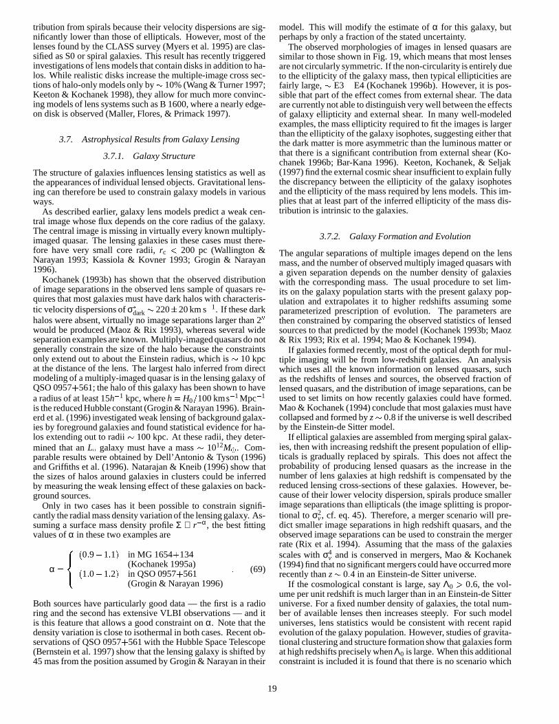
tribution from spirals because their velocity dispersions are sig-nificantly lower than those of ellipticals. However, most of thelenses found by the CLASS survey (Myers et al. 1995) are clas-sified as S0 or spiral galaxies. This result has recently triggeredinvestigations of lens models that contain disks in addition to ha-los. While realistic disks increase the multiple-image cross sec-tions of halo-only models only by 10% (Wang & Turner 1997;Keeton & Kochanek 1998), they allow for much more convinc-ing models of lens systems such as B 1600, where a nearly edge-on disk is observed (Maller, Flores, & Primack 1997).

3.7. Astrophysical Results from Galaxy Lensing

3.7.1. Galaxy Structure

The structure of galaxies influences lensing statistics as well asthe appearances of individual lensed objects. Gravitational lens-ing can therefore be used to constrain galaxy models in variousways.

As described earlier, galaxy lens models predict a weak cen-tral image whose flux depends on the core radius of the galaxy.The central image is missing in virtually every known multiply-imaged quasar. The lensing galaxies in these cases must there-fore have very small core radii, rc < 200 pc (Wallington &Narayan 1993; Kassiola & Kovner 1993; Grogin & Narayan1996).

Kochanek (1993b) has shown that the observed distributionof image separations in the observed lens sample of quasars re-quires that most galaxies must have dark halos with characteris-tic velocity dispersions of σdark 22020 km s1. If these darkhalos were absent, virtually no image separations larger than 200

would be produced (Maoz & Rix 1993), whereas several wideseparation examples are known. Multiply-imaged quasars do notgenerally constrain the size of the halo because the constraintsonly extend out to about the Einstein radius, which is 10 kpcat the distance of the lens. The largest halo inferred from directmodeling of a multiply-imaged quasar is in the lensing galaxy ofQSO 0957+561; the halo of this galaxy has been shown to havea radius of at least 15h1 kpc, where h = H0=100 kms1 Mpc1

is the reduced Hubble constant (Grogin & Narayan 1996). Brain-erd et al. (1996) investigated weak lensing of background galax-ies by foreground galaxies and found statistical evidence for ha-los extending out to radii 100 kpc. At these radii, they deter-mined that an L galaxy must have a mass 1012M. Com-parable results were obtained by Dell’Antonio & Tyson (1996)and Griffiths et al. (1996). Natarajan & Kneib (1996) show thatthe sizes of halos around galaxies in clusters could be inferredby measuring the weak lensing effect of these galaxies on back-ground sources.

Only in two cases has it been possible to constrain signifi-cantly the radial mass density variation of the lensing galaxy. As-suming a surface mass density profile Σ ∝ rα, the best fittingvalues of α in these two examples are

α =

8><>:

(0:91:1) in MG 1654+134(Kochanek 1995a)

(1:01:2) in QSO 0957+561(Grogin & Narayan 1996)

: (69)

Both sources have particularly good data — the first is a radioring and the second has extensive VLBI observations — and itis this feature that allows a good constraint on α. Note that thedensity variation is close to isothermal in both cases. Recent ob-servations of QSO 0957+561 with the Hubble Space Telescope(Bernstein et al. 1997) show that the lensing galaxy is shifted by45 mas from the position assumed by Grogin & Narayan in their

model. This will modify the estimate of α for this galaxy, butperhaps by only a fraction of the stated uncertainty.

The observed morphologies of images in lensed quasars aresimilar to those shown in Fig. 19, which means that most lensesare not circularly symmetric. If the non-circularity is entirely dueto the ellipticity of the galaxy mass, then typical ellipticities arefairly large, E3E4 (Kochanek 1996b). However, it is pos-sible that part of the effect comes from external shear. The dataare currently not able to distinguish very well between the effectsof galaxy ellipticity and external shear. In many well-modeledexamples, the mass ellipticity required to fit the images is largerthan the ellipticity of the galaxy isophotes, suggesting either thatthe dark matter is more asymmetric than the luminous matter orthat there is a significant contribution from external shear (Ko-chanek 1996b; Bar-Kana 1996). Keeton, Kochanek, & Seljak(1997) find the external cosmic shear insufficient to explain fullythe discrepancy between the ellipticity of the galaxy isophotesand the ellipticity of the mass required by lens models. This im-plies that at least part of the inferred ellipticity of the mass dis-tribution is intrinsic to the galaxies.

3.7.2. Galaxy Formation and Evolution

The angular separations of multiple images depend on the lensmass, and the number of observed multiply imaged quasars witha given separation depends on the number density of galaxieswith the corresponding mass. The usual procedure to set lim-its on the galaxy population starts with the present galaxy pop-ulation and extrapolates it to higher redshifts assuming someparameterized prescription of evolution. The parameters arethen constrained by comparing the observed statistics of lensedsources to that predicted by the model (Kochanek 1993b; Maoz& Rix 1993; Rix et al. 1994; Mao & Kochanek 1994).

If galaxies formed recently, most of the optical depth for mul-tiple imaging will be from low-redshift galaxies. An analysiswhich uses all the known information on lensed quasars, suchas the redshifts of lenses and sources, the observed fraction oflensed quasars, and the distribution of image separations, can beused to set limits on how recently galaxies could have formed.Mao & Kochanek (1994) conclude that most galaxies must havecollapsed and formed by z 0:8 if the universe is well describedby the Einstein-de Sitter model.

If elliptical galaxies are assembled from merging spiral galax-ies, then with increasing redshift the present population of ellip-ticals is gradually replaced by spirals. This does not affect theprobability of producing lensed quasars as the increase in thenumber of lens galaxies at high redshift is compensated by thereduced lensing cross-sections of these galaxies. However, be-cause of their lower velocity dispersion, spirals produce smallerimage separations than ellipticals (the image splitting is propor-tional to σ2

v , cf. eq. 45). Therefore, a merger scenario will pre-dict smaller image separations in high redshift quasars, and theobserved image separations can be used to constrain the mergerrate (Rix et al. 1994). Assuming that the mass of the galaxiesscales with σ4

v and is conserved in mergers, Mao & Kochanek(1994) find that no significant mergers could have occurred morerecently than z 0:4 in an Einstein-de Sitter universe.

If the cosmological constant is large, say Λ0 > 0:6, the vol-ume per unit redshift is much larger than in an Einstein-de Sitteruniverse. For a fixed number density of galaxies, the total num-ber of available lenses then increases steeply. For such modeluniverses, lens statistics would be consistent with recent rapidevolution of the galaxy population. However, studies of gravita-tional clustering and structure formation show that galaxies format high redshifts precisely when Λ0 is large. When this additionalconstraint is included it is found that there is no scenario which

19

allows recent galaxy formation or evolution in the universe (seealso Sect. 3.7.5.).

Since lensing statistics are fully consistent with the known lo-cal galaxy population extrapolated to redshifts z 1, the num-ber densities of any dark “failed” galaxies are constrained quitestrongly. As a function of velocity dispersion σ, the current con-straints are (Mao & Kochanek 1994)

ndark <

8<:

0:15h3 Mpc3 for σ = 100 km s1

0:032h3 Mpc3 for σ = 150 km s1

0:017h3 Mpc3 for σ = 200 km s1: (70)

3.7.3. Constraint on CDM

The popular cold dark matter (CDM) scenario of structure for-mation in its “standard” variant (Ω0 = 1, Λ0 = 0 and COBE nor-malized) predicts the formation of large numbers of dark mat-ter halos in the mass range between galaxies and galaxy clus-ters. The implications of these halos for lensing were consid-ered by Narayan & White (1988) and more recently by Cen etal. (1994); Wambsganss et al. (1995); Wambsganss, Cen, & Os-triker (1998); and Kochanek (1995b). The latter authors haveshown quite convincingly that the standard CDM model pro-duces many more wide-separation quasar pairs than observed.For example, a recent search of a subsample of the HST snap-shot survey for multiply imaged QSOs with image separationsbetween 700 and 5000 found a null result (Maoz et al. 1997). Tosave CDM, either the normalization of the model needs to bereduced to σ8 0:5 0:2, or the long-wavelength slope of thepower spectrum needs to be lowered to n 0:5 0:2. Both ofthese options are inconsistent with the COBE results. The prob-lem of the over-productionof wide angle pairs is just a manifesta-tion of the well-known problem that standard COBE-normalizedCDM over-produces cluster-scale mass condensations by a largefactor. Models which are adjusted to fit the observed numberdensity of clusters also satisfy the gravitational lens constraint.

If the dark halos have large core radii, their central densitycould drop below the critical value for lensing and this wouldreduce the predicted number of wide-separation lens systems.Large core radii thus may save standard CDM (Flores & Primack1996), but there is some danger of fine-tuning in such an expla-nation. As discussed in Sect. 3.7.1., galaxy cores are quite small.Therefore, one needs to invoke a rather abrupt increase of coreradius with increasing halo mass.

3.7.4. Hubble Constant

The lens equation is dimensionless, and the positions of im-ages as well as their magnifications are dimensionless numbers.Therefore, information on the image configuration alone doesnot provide any constraint on the overall scale of the lens geom-etry or the value of the Hubble constant. Refsdal (1964) realizedthat the time delay, however, is proportional to the absolute scaleof the system and does depend on H0 (cf. Fig. 22).

To see this, we first note that the geometrical time delay is sim-ply proportional to the path lengths of the rays which scale asH1

0 . The potential time delay also scales as H10 because the

linear size of the lens and its mass have this scaling. Therefore,for any gravitational lens system, the quantity

H0 ∆τ (71)

depends only on the lens model and the geometry of the system.A good lens model which reproduces the positions and magni-fications of the images provides the scaled time delay H0 ∆τ be-tween the images. Therefore, a measurement of the time delay∆τ will yield the Hubble constant H0 (Refsdal 1964, 1966a).

FIG. 22.—Sketch of the dependence of the overall scale of a lens systemon the value of the Hubble constant.

To measure the time delay, the fluxes of the images need to bemonitored over a period of time significantly longer than the timedelay in order to achieve reasonable accuracy. In fact, the analy-sis of the resulting light curves is not straightforward because ofuneven data sampling, and careful and sophisticated data analy-sis techniques have to be applied. QSO 0957+561 has beenmonitored both in the optical (Vanderriest et al. 1989; Schild &Thomson 1993; Kundic et al. 1996) and radio wavebands (Leharet al. 1992; Haarsma et al. 1996, 1997). Unfortunately, analysisof the data has led to two claimed time delays:

∆τ = (1:480:03) years (72)

(Press, Rybicki, & Hewitt 1992a,b) and

∆τ' 1:14 years (73)

(Schild & Thomson 1993; Pelt et al. 1994, 1996). The discrep-ancy appears to have been resolved in favor of the shorter delay.Haarsma et al. (1996) find ∆τ = 1:031:33years, and Kundic etal. (1996) derive ∆τ = 4173days using a variety of statisticaltechniques.

In addition to a measurement of the time delay, it is also neces-sary to develop a reliable model to calculate the value of H0∆τ.QSO 0957+561 has been studied by a number of groups overthe years, with recent work incorporating constraints from VLBIimaging (Falco et al. 1991). Grogin & Narayan (1996) estimatethe Hubble constant to be given by

H0 = (826)(1κ)

∆τ1:14 yr

1

kms1 Mpc1 (74)

where κ refers to the unknown convergence due to the clustersurrounding the lensing galaxy. Since the cluster κ cannot benegative, this result directly gives an upper bound on the Hub-ble constant (H0 < 88 kms1 Mpc1 for ∆τ = 1:14 years). Ac-tually, κ can also be modified by large scale structure along the

20

line of sight. In contrast to the effect of the cluster, this fluctu-ation can have either sign, but the rms amplitude is estimatedto be only a few per cent (Seljak 1994; Bar-Kana 1996). Surpi,Harari, & Frieman (1996) confirm that large-scale structure doesnot modify the functional relationship between lens observables,and therefore does not affect the determination of H0.

To obtain an actual value of H0 instead of just an upper bound,we need an independent estimate of κ. Studies of weak lensingby the cluster (Fischer et al. 1997) give κ = 0:24 0:12 (2σ)at the location of the lens (cf. Kundic et al. 1996). This corre-sponds to H0 = 62+12

13 kms1 Mpc1. Another technique is tomeasure the velocity dispersion σgal of the lensing galaxy, fromwhich it is possible to estimate κ (Falco et al. 1992; Grogin &Narayan 1996). Falco et al. (1997) used the Keck telescope tomeasure σgal = 279 12 kms1, which corresponds to H0 =

667 kms1 Mpc1. Although most models of QSO 0957+561are based on a spherically symmetric galaxy embedded in an ex-ternal shear (mostly due to the cluster), introduction of ellipticityin the galaxy, or a point mass at the galaxy core, or substructurein the cluster seem to have little effect on the estimate of H0 (Gro-gin & Narayan 1996).

A measurement of the time delay has also been attempted inthe Einstein ring system B 0218+ 357. In this case, a singlegalaxy is responsible for the small image splitting of 0:003. Thetime delay has been determined to be 123 days (1σ confidencelimit) which translates to H0 60 kms1 Mpc1 (Corbett et al.1996).

Schechter et al. (1997) recently announced a time delay of∆τ = 23:73:4days between images B and C of the quadruplelens PG 1115+080. Using a different statistical technique, Bar-Kana (1997) finds ∆τ= 25:0+3:3

3:8 days (95% confidence) from thesame data. Their best fitting lens model, where the lens galaxyas well as an associated group of galaxies are modeled as singu-lar isothermal spheres, gives H0 = 42 6kms1 Mpc1. Othermodels give larger values of H0 but fit the data less well. Kee-ton & Kochanek (1997) have considered a more general class ofmodels where the lensing galaxy is permitted to be elliptical, andpresent a family of models which fit the PG 1115+080 data well.They estimate H0 = 6017kms1 Mpc1. With more accuratedata on the position of the lens galaxy, this estimate could be im-proved to H0 = 53+10

7 kms1 Mpc1 (Courbin et al. 1997).The determination of H0 through gravitational lensing has a

number of advantages over other techniques.

1 The method works directly with sources at large redshifts,z 0:5, whereas most other methods are local (observationswithin 100 Mpc) where peculiar velocities are still com-parable to the Hubble flow.

2 While other determinations of the Hubble constant rely ondistance ladders which progressively reach out to increasingdistances, the measurement via gravitational time delay isa one-shot procedure. One measures directly the geometri-cal scale of the lens system. This means that the lens-basedmethod is absolutely independent of every other methodand at the very least provides a valuable test of other deter-minations.

3 The lens-based method is based on fundamental physics(the theory of light propagation in General Relativity),which is fully tested in the relevant weak-field limit ofgravity. Other methods rely on models for variable stars(Cepheids) or supernova explosions (Type II), or empiri-cal calibrations of standard candles (Tully-Fisher distances,Type I supernovae). The lensing method does require some

information on the “shapes” of galaxies which is used toguide the choice of a parameterized lens model.

3.7.5. Cosmological Constant

A large cosmological constant Λ0 increases the volume per unitredshift of the universe at high redshift. As Turner (1990) re-alized, this means that the relative number of lensed sourcesfor a fixed comoving number density of galaxies increasesrapidly with increasing Λ0. Turning this around it is pos-sible to use the observed probability of lensing to constrainΛ0. This method has been applied by various authors (Turner1990; Fukugita & Turner 1991; Fukugita et al. 1992; Maoz& Rix 1993; Kochanek 1996a), and the current limit is Λ0 <0:65 (2σ confidence limit) for a universe with Ω0 + Λ0 = 1.With a combined sample of optical and radio lenses, this limitcould be slightly improved to Λ0 < 0:62 (2σ; Falco, Kochanek,& Munoz 1998). Malhotra, Rhoads, & Turner (1996) claim thatthere is evidence for considerable amounts of dust in lensinggalaxies. They argue that the absorption in dusty lenses can rec-oncile a large cosmological constant with the observed multiple-image statistics.

A completely independent approach (Kochanek 1992) consid-ers the redshift distribution of lenses. For a given source redshift,the probability distribution of zd peaks at higher redshift with in-creasing Λ0. Once again, by comparing the observations againstthe predicted distributions one obtains an upper limit on Λ0. Thismethod is less sensitive than the first, but gives consistent results.

Another technique consists in comparing the observed QSOimage separations to those expected from the redshifts of lensesand sources and the magnitudes of the lenses, assuming certainvalues for Ω0 and Λ0. The cosmological parameters are then var-ied to optimize the agreement with the observations. Applyingthis approach to a sample of seven lens systems, Im, Griffiths,& Ratnatunga (1997) find Λ0 = 0:64+0:15

0:26 (1σ confidence limit)assuming Ω0 +Λ0 = 1.

4. LENSING BY GALAXY CLUSTERS AND LARGE-SCALESTRUCTURE

Two distinct types of lensing phenomena are observed with clus-ters of galaxies (Fig. 23):

1 Rich centrally condensed clusters occasionally produce gi-ant arcs when a background galaxy happens to be alignedwith one of the cluster caustics. These instances of lens-ing are usually analyzed with techniques similar to those de-scribed in Sect. 2. for galaxy lenses. In brief, a parameter-ized lens model is optimized so as to obtain a good fit to theobserved image.

2 Every cluster produces weakly distorted images of largenumbers of background galaxies. These images are calledarclets and the phenomenon is referred to as weak lensing.With the development of the Kaiser & Squires (1993) algo-rithm and its variants, weak lensing is being used increas-ingly to derive parameter-free two-dimensional mass mapsof lensing clusters.

In addition to these two topics, we also discuss in this sec-tion weak lensing by large-scale structure in the universe. Thistopic promises to develop into an important branch of gravita-tional lensing, and could in principle provide a direct measure-ment of the primordial power spectrum P(k) of the density fluc-tuations in the universe.

21

FIG. 23.—Hubble Space Telescope image of the cluster Abell 2218,showing a number of arcs and arclets around the two centers of the clus-ter. (NASA HST Archive)

4.1. Strong Lensing by Clusters — Giant Arcs

4.1.1. Basic Optics

We begin by summarizing a few features of generic lenses whichwe have already discussed in the previous sections. A lens isfully characterized by its surface mass density Σ(~θ). Strong lens-ing, which is accompanied by multiple imaging, requires that thesurface mass density somewhere in the lens should be larger thanthe critical surface mass density,

Σ& Σcr = 0:35 gcm3

DGpc

1

; (75)

where D is the effective lensing distance defined in eq. (18). Alens which satisfies this condition produces one or more caus-tics. Examples of the caustics produced by an elliptical lens witha finite core are shown in Fig. 19. Sources outside all caus-tics produce a single image; the number of images increases bytwo upon each caustic crossing toward the lens center. As il-lustrated in Figs. 19 and 20, extended sources like galaxies pro-duce large arcs if they lie on top of caustics. The largest arcs areformed from sources on cusp points, because then three imagesof a source merge to form the arc (cf. the right panel in Fig. 19 orthe top right panel in Fig. 20). At the so-called “lips” and “beak-to-beak” caustics, which are related to cusps, similarly large arcsare formed. Sources on a fold caustic give rise to two rather thanthree merging images and thus form moderate arcs.

4.1.2. Cluster Mass Inside a Giant Arc

The location of an arc in a cluster provides a simple way to esti-mate the projected cluster mass within a circle traced by the arc(cf. Fig. 24). For a circularly symmetric lens, the average sur-face mass density hΣi within the tangential critical curve equalsthe critical surface mass density Σcr. Tangentially oriented largearcs occur approximately at the tangential critical curves. The ra-dius θarc of the circle traced by the arc therefore gives an estimateof the Einstein radius θE of the cluster.

Thus we have

hΣ(θarc)i hΣ(θE)i= Σcr ; (76)

and we obtain for the mass enclosed by θ = θarc

M(θ) = Σcr π(Ddθ)2 1:11014 M

θ

3000

2 D1Gpc

:

(77)

FIG. 24.—Tangential arcs constrain the cluster mass within a circletraced by the arcs.

Assuming an isothermal model for the mass distribution in thecluster and using eq. (45), we obtain an estimate for the velocitydispersion of the cluster,

σv 103 kms1

θ2800

1=2 Ds

Dds

1=2

: (78)

In addition to the lensing technique, two other methods are avail-able to obtain the mass of a cluster: the observed velocity disper-sion of the cluster galaxies can be combined with the virial the-orem to obtain one estimate, and observations of the X-ray gascombined with the condition of hydrostatic equilibrium providesanother. These three quite independent techniques yield masseswhich agree with one another to within a factor 23.

The mass estimate (77) is based on very simple assumptions.It can be improved by modeling the arcs with parameterized lensmass distributions and carrying out more detailed fits of the ob-served arcs. We list in Tab. 3 masses, mass-to-blue-light ratios,and velocity dispersions of three clusters with prominent arcs.Additional results can be found in the review article by Fort &Mellier (1994).

4.1.3. Asphericity of Cluster Mass

The fact that the observed giant arcs never have counter-arcsof comparable brightness, and rarely have even small counter-arcs, implies that the lensing geometry has to be non-spherical(Grossman & Narayan 1988; Kovner 1989; see also Figs. 19 and20). Cluster potentials therefore must have substantial quadru-pole and perhaps also higher multipole moments. In the case ofA 370, for example, there are two cD galaxies, and the potentialquadrupole estimated from their separation is consistent with thequadrupole required to model the observed giant arc (Grossman& Narayan 1989). The more detailed model of A 370 by Kneibet al. (1993) shows a remarkable agreement between the lensingpotential and the strongly aspheric X-ray emission of the cluster.

22

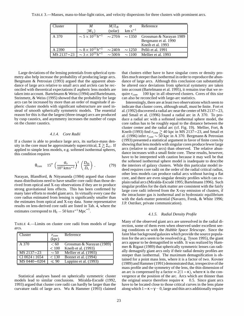
TABLE 3.—Masses, mass-to-blue-light ratios, and velocity dispersions for three clusters with prominent arcs.

Cluster M M=LB σ Reference(M) (solar) km s1

A 370 51013 h1 270h 1350 Grossman & Narayan 1989Bergmann et al. 1990Kneib et al. 1993

A 2390 81013 h1 240h 1250 Pello et al. 1991MS 213723 31013 h1 500h 1100 Mellier et al. 1993

Large deviations of the lensing potentials from spherical sym-metry also help increase the probability of producing large arcs.Bergmann & Petrosian (1993) argued that the apparent abun-dance of large arcs relative to small arcs and arclets can be rec-onciled with theoretical expectations if aspheric lens models aretaken into account. Bartelmann & Weiss (1994) and Bartelmann,Steinmetz, & Weiss (1995) showed that the probability for largearcs can be increased by more than an order of magnitude if as-pheric cluster models with significant substructure are used in-stead of smooth spherically symmetric models. The essentialreason for this is that the largest (three-image) arcs are producedby cusp caustics, and asymmetry increases the number of cuspson the cluster caustics.

4.1.4. Core Radii

If a cluster is able to produce large arcs, its surface-mass den-sity in the core must be approximately supercritical, Σ & Σcr. Ifapplied to simple lens models, e.g. softened isothermal spheres,this condition requires

θcore . 1500 σv

103 kms1

2

Dds

Ds

: (79)

Narayan, Blandford, & Nityananda (1984) argued that clustermass distributions need to have smaller core radii than those de-rived from optical and X-ray observations if they are to producestrong gravitational lens effects. This has been confirmed bymany later efforts to model giant arcs. In virtually every case thecore radius estimated from lensing is significantly smaller thanthe estimates from optical and X-ray data. Some representativeresults on lens-derived core radii are listed in Tab. 4, where theestimates correspond to H0 = 50 kms1 Mpc

1.

TABLE 4.—Limits on cluster core radii from models of largearcs.

Cluster rcore Reference(kpc)

A 370 < 60 Grossman & Narayan (1989)< 100 Kneib et al. (1993)

MS 213723 50 Mellier et al. (1993)Cl 0024+1654 < 130 Bonnet et al. (1994)MS 0440+0204 90 Luppino et al. (1993)

Statistical analyses based on spherically symmetric clustermodels lead to similar conclusions. Miralda-Escude (1992,1993) argued that cluster core radii can hardly be larger than thecurvature radii of large arcs. Wu & Hammer (1993) claimed

that clusters either have to have singular cores or density pro-files much steeper than isothermal in order to reproduce the abun-dance of large arcs. Although this conclusion can substantiallybe altered once deviations from spherical symmetry are takeninto account (Bartelmann et al. 1995), it remains true that we re-quire rcore . 100 kpc in all observed clusters. Cores of this sizecan also be reconciled with large-arc statistics.

Interestingly, there are at least two observations which seem toindicate that cluster cores, although small, must be finite. Fort etal. (1992) discovered a radial arc near the center of MS 213723,and Smail et al. (1996) found a radial arc in A 370. To pro-duce a radial arc with a softened isothermal sphere model, thecore radius has to be roughly equal to the distance between thecluster center and the radial arc (cf. Fig. 19). Mellier, Fort, &Kneib (1993) find rcore & 40 kpc in MS 213723, and Smail etal. (1996) infer rcore 50 kpc in A 370. Bergmann & Petrosian(1993) presented a statistical argument in favor of finite cores byshowing that lens models with singular cores produce fewer largearcs (relative to small arcs) than observed. The relative abun-dance increases with a small finite core. These results, however,have to be interpreted with caution because it may well be thatthe softened isothermal sphere model is inadequate to describethe interiors of galaxy clusters. While this particular model in-deed requires core radii on the order of the radial critical radius,other lens models can produce radial arcs without having a flatcore, and there are even singular density profiles which can ex-plain radial arcs (Miralda-Escude 1995; Bartelmann 1996). Suchsingular profiles for the dark matter are consistent with the fairlylarge core radii inferred from the X-ray emission of clusters, ifthe intracluster gas is isothermal and in hydrostatic equilibriumwith the dark-matter potential (Navarro, Frenk, & White 1996;J.P. Ostriker, private communication).

4.1.5. Radial Density Profile

Many of the observed giant arcs are unresolved in the radial di-rection, some of them even when observed under excellent see-ing conditions or with the Hubble Space Telescope. Since thefaint blue background galaxies which provide the source popula-tion for the arcs seem to be resolved (e.g. Tyson 1995), the giantarcs appear to be demagnified in width. It was realized by Ham-mer & Rigaut (1989) that spherically symmetric lenses can radi-ally demagnify giant arcs only if their radial density profiles aresteeper than isothermal. The maximum demagnification is ob-tained for a point mass lens, where it is a factor of two. Kovner(1989) and Hammer (1991) demonstrated that, irrespective of themass profile and the symmetry of the lens, the thin dimension ofan arc is compressed by a factor 2(1κ), where κ is the con-vergence at the position of the arc. Arcs which are thinner thanthe original source therefore require κ . 0:5. Since giant arcshave to be located close to those critical curves in the lens planealong which 1κγ= 0, large and thin arcs additionally require

23

γ& 0:5.In principle, the radius of curvature of large arcs relative to

their distance from the cluster center can be used to constrainthe steepness of the radial density profile (Miralda-Escude 1992,1993), but results obtained from observed arcs are not yet con-clusive (Grossman & Saha 1994). One problem with this methodis that substructure in clusters tends to enlarge curvature radii ir-respective of the mass profile of the dominant component of thecluster (Miralda-Escude 1993; Bartelmann et al. 1995).

Wu & Hammer (1993) argued for steep mass profiles on statis-tical grounds because the observed abundance of large arcs ap-pears to require highly centrally condensed cluster mass profilesin order to increase the central mass density of clusters whilekeeping their total mass constant. However, their conclusionsare based on spherically symmetric lens models and are sig-nificantly changed when the symmetry assumption is dropped(Bartelmann et al. 1995).

It should also be kept in mind that not all arcs are thin. Some“thick” and resolved arcs are known (e.g. in A 2218, Pello-Descayre et al. 1988; and in A 2390, Pello et al. 1991), and itis quite possible that thin arcs predominate just because they aremore easily detected than thick ones due to observational selec-tion effects. Also, Miralda-Escude (1992, 1993) has argued thatintrinsic source ellipticity can increase the probability of produc-ing thin arcs, while Bartelmann et al. (1995) showed that the con-dition κ . 0:5 which is required for thin arcs can be more fre-quently fulfilled in clusters with substructure where the shear islarger than in spherically symmetric clusters.

4.1.6. Mass Sub-Condensations

The cluster A 370 has two cD galaxies and is a clear exampleof a cluster with multiple mass centers. A two-component massmodel centered on the cD galaxies (Kneib et al. 1993) fits verywell the lens data as well as X-ray and deep optical images of thecluster. Abell 2390 is an interesting example because it containsa “straight arc” (Pello et al. 1991, see also Mathez et al. 1992)which can be produced only with either a lips or a beak-to-beakcaustic (Kassiola, Kovner, & Blandford 1992). If the arc is mod-eled with a lips caustic, it requires the mass peak to be close to thelocation of the arc, but this is not where the cluster light is cen-tered. With a beak-to-beak caustic, the model requires two sep-arate mass condensations, one of which could be at the peak ofthe luminosity, but then the other has to be a dark condensation.Pierre et al. (1996) find enhanced X-ray emission at a plausibleposition of the secondary mass clump, and from a weak lensinganalysis Squires et al. (1996b) find a mass map which is consis-tent with a mass condensation at the location of the enhanced X-ray emission.

Abell 370 and A 2390 are the most obvious examples of whatis probably a widespread phenomenon, namely that clusters arein general not fully relaxed but have substructure as a result ofongoing evolution. If clusters are frequently clumpy, this canlead to systematic effects in the statistics of arcs and in the de-rived cluster parameters (Bartelmann et al. 1995; Bartelmann1995b).

4.1.7. Lensing Results vs. Other Mass Determinations

Enclosed Mass Three different methods are currently used toestimate cluster masses. Galaxy velocity dispersions yield amass estimate from the virial theorem, and hence the galaxieshave to be in virial equilibrium for such estimates to be valid. Itmay also be that the velocities of cluster galaxies are biased rela-tive to the velocities of the dark matter particles (Carlberg 1994),though current estimates suggest that the bias is no more than

about 10%. The X-ray emission of rich galaxy clusters is domi-nated by free-free emission of thermal electrons and therefore de-pends on the squared density of the intracluster gas, which in turntraces the gravitational potential of the clusters. Such estimatesusually assume that the cluster gas is in thermal hydrostatic equi-librium and that the potential is at least approximately spheri-cally symmetric. Finally, large arcs in clusters provide a massestimate through eq. (77) or by more detailed modeling. Thesethree mass estimates are in qualitative agreement with each otherup to factors of 23.

Miralda-Escude & Babul (1995) compared X-ray and large-arc mass estimates for the clusters A 1689, A 2163 and A 2218.They took into account deviations from spherical symmetry andobtained lensing masses from individual lens models which re-produce the observed arcs. They arrived at the conclusion thatin A 1689 and A 2218 the mass required for producing the largearcs is higher by a factor of 2 2:5 than the mass required forthe X-ray emission, and proposed a variety of reasons for sucha discrepancy, among them projection effects and non-thermalpressure support. Loeb & Mao (1994) specifically suggestedthat strong turbulence and magnetic fields in the intracluster gasmay constitute a significant non-thermal pressure component inA 2218 and thus render the X-ray mass estimate too low. Bartel-mann & Steinmetz (1996) used gas dynamical cluster simula-tions to compare their X-ray and lensing properties. They founda similar discrepancy as that identified by Miralda-Escude &Babul (1995) in those clusters that show structure in the distribu-tion of line-of-sight velocities of the cluster particles, indicativeof merging or infall along the line-of-sight. The discrepancy isprobably due to projection effects.

Bartelmann (1995b) showed that cluster mass estimates ob-tained from large arcs by straightforward application of eq. (77)are systematically too high by a factor of 1:6 on average, andby as much as a factor of 2 in 1 out of 5 cases. This discrepancyarises because eq. (77) assumes a smooth spherically symmetricmass distribution whereas realistic clusters are asymmetric andhave substructure. Note that Daines et al. (1996) found evidencefor two or more mass condensations along the line of sight to-ward A 1689, while the arclets in A 2218 show at least two massconcentrations. It appears that cluster mass estimates from lens-ing require detailed lens models in order to be accurate to betterthan 30 50 per cent. In the case of MS 1224, Fahlman etal. (1994) and Carlberg, Yee, & Ellingson (1994) have obtainedmasses using the Kaiser & Squires weak-lensing cluster recon-struction method. Their mass estimates are 2 3 times higherthan the cluster’s virial mass. Carlberg et al. find evidence fromvelocity measurements that there is a second poor cluster in theforeground of MS 1224 which may explain the result. All ofthese mass discrepancies illustrate that cluster masses must stillbe considered uncertain to a factor of 2 in general.

Core Radii Lensing estimates of cluster core radii are gener-ally much smaller than the core radii obtained from optical orX-ray data. The upper limits on the core radii from lensing arefairly robust and probably reliable. Many clusters with large arcshave cD galaxies which can steepen the central mass profile ofthe cluster. However, there are also non-cD clusters with giantarcs, e.g. A 1689 and Cl 1409 (Tyson 1990), and MS 0440+02(Luppino et al. 1993). In fact, Tyson (1990) claims that thesetwo clusters have cores smaller than 100h1 kpc, similar to up-per limits for core radii found in other arc clusters with cD galax-ies. As mentioned in Sect. 4.1.4., even the occurrence of radialarcs in clusters does not necessarily require a non-singular core,and so all the lensing data are consistent with singular cores inclusters. The X-ray core radii depend on whether or not the cool-ing regions of clusters are included in the emissivity profile fits,

24

because the cooling radii are of the same order of magnitudeas the core radii. If cooling is included, the best-fit core radiiare reduced by a factor of ' 4 (Gerbal et al. 1992; Durret et al.1994). Also, isothermal gas in hydrostatic equilibrium in a sin-gular dark-matter distribution develops a flat core with a core ra-dius similar to those observed. Therefore, the strongly peakedmass distributions required for lensing seem to be quite compat-ible with the extended X-ray cores observed.

Does Mass Follow Light? Leaving the core radius aside, doesmass follow light? It is clear that the mass cannot be as concen-trated within the galaxies as the optical light is (e.g. Bergmann,Petrosian, & Lynds 1990). However, if the optical light issmoothed and assumed to trace the mass, then the resulting massdistribution is probably not very different from the true mass dis-tribution. For instance, in A 370, the elongation of the mass dis-tribution required for the giant arc is along the line connectingthe two cD galaxies in the cluster (Grossman & Narayan 1989)and in fact Kneib et al. (1993) are able to achieve an excellent fitof the giant arc and several arclets with two mass concentrationssurrounding the two cDs. Their model potential also agrees verywell with the X-ray emission of the cluster. In MS 2137, the opti-cal halo is elongated in the direction indicated by the arcs for theoverall mass asymmetry (Mellier et al. 1993), and in Cl 0024, themass distribution is elongated in the same direction as the galaxydistribution (Wallington, Kochanek, & Koo 1995). Smail et al.(1995) find that the mass maps of two clusters reconstructed fromweak lensing agree fairly well with their X-ray emission. An im-portant counterexample is the cluster A 2390, where the straightarc requires a mass concentration which is completely dark in theoptical (Kassiola et al. 1992). Pierre et al. (1996), however, findexcess X-ray emission at a position compatible with the arc.

What Kinds of Clusters Produce Giant Arcs? Which para-meters determine whether or not a galaxy cluster is able to pro-duce large arcs? Clearly, large velocity dispersions and smallcore radii favor the formation of arcs. As argued earlier, intrinsicasymmetries and substructure also increase the ability of clustersto produce arcs because they increase the shear and the numberof cusps in the caustics.

The abundance of arcs in X-ray luminous clusters appears tobe higher than in optically selected clusters. At least a quarter,maybe half, of the 38 X-ray bright clusters selected by Le Fevreet al. (1994) contain large arcs, while Smail et al. (1991) foundonly one large arc in a sample of 19 distant optically selectedclusters. However, some clusters which are prominent lenses(A 370, A 1689, A 2218) are moderate X-ray sources, whileother clusters which are very luminous X-ray sources (A 2163,Cl 1455) are poor lenses. The correlation between X-ray bright-ness and enhanced occurrence of arcs may suggest that X-raybright clusters are more massive and/or more centrally con-densed than X-ray quiet clusters.

Substructure appears to be at least as important as X-raybrightness for producing giant arcs. For example, A 370, A 1689and A 2218 all seem to have clumpy mass distributions. Bartel-mann & Steinmetz (1996) used numerical cluster simulations toshow that the optical depth for arc formation is dominated byclusters with intermediate rather than the highest X-ray luminosi-ties.

Another possibility is that giant arcs preferentially form inclusters with cD galaxies. A 370, for instance, even has twocDs. However, non-cD clusters with giant arcs are known, e.g.A 1689, Cl 1409 (Tyson et al. 1990), and MS 0440+02 (Luppinoet al. 1993).

4.2. Weak Lensing by Clusters — Arclets

In addition to the occasional giant arc, which is produced whena source happens to straddle a caustic, a lensing cluster also pro-duces a large number of weakly distorted images of other back-ground sources which are not located near caustics. These are thearclets. There is a population of distant blue galaxies in the uni-verse whose spatial density reaches 50100 galaxies per squarearc minute at faint magnitudes (Tyson 1988). Each cluster there-fore has on the order of 50 100 arclets per square arc minuteexhibiting a coherent pattern of distortions. Arclets were first de-tected by Fort et al. (1988).

The separations between arclets, typically (5 10)00, aremuch smaller than the scale over which the gravitational poten-tial of a cluster as a whole changes appreciably. The weak andnoisy signals from several individual arclets can therefore be av-eraged by statistical techniques to get an idea of the mass dis-tribution of a cluster. This technique was first demonstrated byTyson, Valdes, & Wenk (1990). Kochanek (1990) and Miralda-Escude (1991a) studied how parameterized cluster lens modelscan be constrained with arclet data.

The first systematic and parameter-free procedure to convertthe observed ellipticities of arclet images to a surface densitymap Σ(~θ) of the lensing cluster was developed by Kaiser &Squires (1993). An ambiguity intrinsic to all such inversionmethods which are based on shear information alone was iden-tified by Seitz & Schneider (1995a). This ambiguity can be re-solved by including information on the convergence of the clus-ter; methods for this were developed by Broadhurst, Taylor, &Peacock (1995) and Bartelmann & Narayan (1995a).

4.2.1. The Kaiser & Squires Algorithm

The technique of Kaiser & Squires (1993) is based on the factthat both convergence κ(~θ) and shear γ1;2(

~θ) are linear combi-nations of second derivatives of the effective lensing potentialψ(~θ). There is thus a mathematical relation connecting the two.In the Kaiser & Squires method one first estimates γ1;2(

~θ) bymeasuring the weak distortions of background galaxy images,and then uses the relation to infer κ(~θ). The surface density ofthe lens is then obtained from Σ(~θ) = Σcrκ(~θ) (see eq. 50).

As shown in Sect. 3., κ and γ1;2 are given by

κ(~θ) =12

∂2ψ(~θ)

∂θ21

+∂2ψ(~θ)

∂θ22

!;

γ1(~θ) =

12

∂2ψ(~θ)

∂θ21

∂2ψ(~θ)∂θ2

2

!;

γ2(~θ) =

∂2ψ(~θ)∂θ1∂θ2

:

(80)

If we introduce Fourier transforms of κ, γ1;2, and ψ (which wedenote by hats on the symbols), we have

κ(~k) = 12(k2

1 + k22)ψ(~k) ;

γ1(~k) = 1

2(k2

1 k22)ψ(~k) ;

γ2(~k) = k1k2ψ(~k) ;

(81)

25

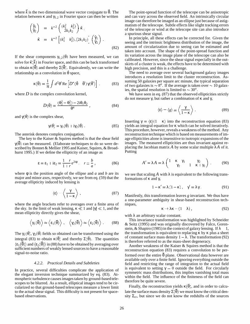
where~k is the two dimensional wave vector conjugate to~θ. Therelation between κ and γ1;2 in Fourier space can then be written

γ1γ2

= k2

(k2

1 k22)

2k1k2

κ ;

κ = k2h(k2

1 k22);(2k1k2)

i γ1γ2

:

(82)

If the shear components γ1;2(~θ) have been measured, we can

solve for κ(~k) in Fourier space, and this can be back transformedto obtain κ(~θ) and thereby Σ(~θ). Equivalently, we can write therelationship as a convolution in~θ space,

κ(~θ) =1π

Zd2θ0Re

hD

(~θ~θ0)γ(~θ0)i; (83)

where D is the complex convolution kernel,

D(~θ) =(θ2

2θ21)2iθ1θ2

θ4 ; (84)

and γ(~θ) is the complex shear,

γ(~θ) = γ1(~θ)+ iγ2(

~θ) : (85)

The asterisk denotes complex conjugation.The key to the Kaiser & Squires method is that the shear field

γ(~θ) can be measured. (Elaborate techniques to do so were de-scribed by Bonnet & Mellier 1995 and Kaiser, Squires, & Broad-hurst 1995.) If we define the ellipticity of an image as

ε = ε1 + iε2 =1 r1+ r

e2iφ ; r ba; (86)

where φ is the position angle of the ellipse and a and b are itsmajor and minor axes, respectively, we see from eq. (59) that theaverage ellipticity induced by lensing is

hεi=

γ1κ

; (87)

where the angle brackets refer to averages over a finite area ofthe sky. In the limit of weak lensing, κ 1 and jγj 1, and themean ellipticity directly gives the shear,D

γ1(~θ)ED

ε1(~θ)E;D

γ2(~θ)ED

ε2(~θ)E: (88)

The γ1(~θ), γ2(

~θ) fields so obtained can be transformed using theintegral (83) to obtain κ(~θ) and thereby Σ(~θ). The quantitieshε1(

~θ)i and hε2(~θ)i in (88) have to be obtained by averaging over

sufficient numbers of weakly lensed sources to have a reasonablesignal-to-noise ratio.

4.2.2. Practical Details and Subtleties

In practice, several difficulties complicate the application ofthe elegant inversion technique summarized by eq. (83). At-mospheric turbulence causes images taken by ground-based tele-scopes to be blurred. As a result, elliptical images tend to be cir-cularized so that ground-based telescopes measure a lower limitto the actual shear signal. This difficulty is not present for space-based observations.

The point-spread function of the telescope can be anisotropicand can vary across the observed field. An intrinsically circularimage can therefore be imaged as an ellipse just because of astig-matism of the telescope. Subtle effects like slight tracking errorsof the telescope or wind at the telescope site can also introducea spurious shear signal.

In principle, all these effects can be corrected for. Given theseeing and the intrinsic brightness distribution of the image, theamount of circularization due to seeing can be estimated andtaken into account. The shape of the point-spread function andits variation across the image plane of the telescope can also becalibrated. However, since the shear signal especially in the out-skirts of a cluster is weak, the effects have to be determined withhigh precision, and this is a challenge.

The need to average over several background galaxy imagesintroduces a resolution limit to the cluster reconstruction. As-suming 50 galaxies per square arc minute, the typical separationof two galaxies is 800. If the average is taken over 10 galax-ies, the spatial resolution is limited to 3000.

We have seen in eq. (87) that the observed ellipticities strictlydo not measure γ, but rather a combination of κ and γ,

hεi= hgi

γ1κ

: (89)

Inserting γ = hεi(1 κ) into the reconstruction equation (83)yields an integral equation for κ which can be solved iteratively.This procedure, however, reveals a weakness of the method. Anyreconstruction technique which is based on measurements of im-age ellipticities alone is insensitive to isotropic expansions of theimages. The measured ellipticities are thus invariant against re-placing the Jacobian matrix A by some scalar multiple λA of it.Putting

A 0 = λA = λ

1κ γ1 γ2γ2 1κ+ γ1

; (90)

we see that scaling A with λ is equivalent to the following trans-formations of κ and γ,

1κ0 = λ(1κ) ; γ0 = λγ : (91)

Manifestly, this transformation leaves g invariant. We thus havea one-parameter ambiguity in shear-based reconstruction tech-niques,

κ! λκ+(1λ) ; (92)

with λ an arbitrary scalar constant.This invariance transformation was highlighted by Schneider

& Seitz (1995) and was originally discovered by Falco, Goren-stein, & Shapiro (1985) in the context of galaxy lensing. If λ. 1,the transformation is equivalent to replacing κ by κ plus a sheetof constant surface mass density 1λ. The transformation (92)is therefore referred to as the mass-sheet degeneracy.

Another weakness of the Kaiser & Squires method is that thereconstruction equation (83) requires a convolution to be per-formed over the entire~θ plane. Observational data however areavailable only over a finite field. Ignoring everything outside thefield and restricting the range of integration to the actual fieldis equivalent to setting γ = 0 outside the field. For circularlysymmetric mass distributions, this implies vanishing total masswithin the field. The influence of the finiteness of the field cantherefore be quite severe.

Finally, the reconstruction yields κ(~θ), and in order to calcu-late the surface mass density Σ(~θ) we must know the critical den-sity Σcr, but since we do not know the redshifts of the sources

26

FIG. 25.—HST image of the cluster Cl 0024, overlaid on the left with the shear field obtained from an observation of arclets with the Canada-France Hawaii Telescope (Y. Mellier & B. Fort), and on the right with the reconstructed surface-mass density determined from the shear field (C.Seitz et al.). The reconstruction was done with a non-linear, finite-field algorithm.

there is a scaling uncertainty in this quantity. For a lens withgiven surface mass density, the distortion increases with increas-ing source redshift. If the sources are at much higher redshiftsthan the cluster, the influence of the source redshift becomesweak. Therefore, this uncertainty is less serious for low redshiftclusters.

Nearly all the problems mentioned above have been addressedand solved. The solutions are discussed in the following subsec-tions.

4.2.3. Eliminating the Mass Sheet Degeneracy by Measuringthe Convergence

By eq. (60),

µ =1

(1κ)2 γ2 ; (93)

and so the magnification scales with λ as µ ∝ λ2. Therefore, themass-sheet degeneracy can be broken by measuring the magnifi-cation µ of the images in addition to the shear (Broadhurst et al.1995). Two methods have been proposed to measure µ. The firstrelies on comparing the galaxy counts in the cluster field withthose in an unlensed “empty” field (Broadhurst et al. 1995). Theobserved counts of galaxies brighter than some limiting magni-tude m are related to the intrinsic counts through

N0(m) = N0(m)µ2:5s1 ; (94)

where s is the logarithmic slope of the intrinsic number countfunction,

s =d logN(m)

dm: (95)

In blue light, s 0:4, and thus N0(m)N(m) independent of themagnification, but in red light s 0:15, and the magnificationleads to a dilution of galaxies behind clusters. The reduction of

red galaxy counts behind the cluster A 1689 has been detectedby Broadhurst (1995).

The other method is to compare the sizes of galaxies in thecluster field to those of similar galaxies in empty fields. Sincelensing conserves surface brightness, it is most convenient tomatch galaxies with equal surface brightness while making thiscomparison (Bartelmann & Narayan 1995a). The magnificationis then simply the ratio between the sizes of lensed and unlensedgalaxies. Labeling galaxies by their surface brightness has thefurther advantage that the surface brightness is a steep functionof galaxy redshift, which allows the user to probe the change oflens efficiency with source redshift (see below).

4.2.4. Determining Source Redshifts

For a given cluster, the strength of distortion and magnificationdue to lensing increases with increasing source redshift zs. Themean redshift zs of sources as a function of apparent magnitude mcan thus be inferred by studying the mean strength of the lensingsignal vs. m (Kaiser 1995; Kneib et al. 1996).

The surface brightness S probably provides a better label forgalaxies than the apparent magnitude because it depends steeplyon redshift and is unchanged by lensing. Bartelmann & Narayan(1995a) have developed an algorithm, which they named the lensparallax method, to reconstruct the cluster mass distributions andto infer simultaneously zs as a function of the surface brightness.In simulations, data from 10 cluster fields and an equal numberof empty comparison fields were sufficient to determine the clus-ter masses to 5% and the galaxy redshifts to 10% accu-racy. The inclusion of galaxy sizes in the iterative lens-parallaxalgorithm breaks the mass-sheet degeneracy, thereby removingthe ambiguities in shear-based cluster reconstruction techniquesarising from the transformation (92) and from the unknown red-shift distribution of the sources.

27

4.2.5. Finite Field Methods

As emphasized previously, the inversion equation (83) requires aconvolution to be performed over the entire real plane. The factthat data are always restricted to a finite field thus introduces a se-vere bias in the reconstruction. Modified reconstruction kernelshave been suggested to overcome this limitation.

Consider the relation (Kaiser 1995)

~∇κ =

γ1;1 + γ2;2γ2;1 γ1;2

: (96)

This shows that the convergence at any point~θ in the data field isrelated by a line integral to the convergence at another point~θ0,

κ(~θ) = κ(~θ0)+

Z ~θ

~θ0

d~l ~∇κ[~θ(~l)] : (97)

If the starting point~θ0 is far from the cluster center, κ(~θ0) maybe expected to be small and can be neglected. For each start-ing point ~θ0, eq. (97) yields an estimate for κ(~θ) κ(~θ0), andby averaging over all chosen~θ0 modified reconstruction kernelscan be constructed (Schneider 1995; Kaiser et al. 1995; Bartel-mann 1995c; Seitz & Schneider 1996). Various choices for theset of starting positions~θ0 have been suggested. For instance,one can divide the observed field into an inner region centeredon the cluster and take as ~θ0 all points in the rest of the field.Another possibility is to take ~θ0 from the entire field. In bothcases, the result is κ(~θ) κ, where κ is the average convergencein the region from which the points~θ0 were chosen. The averageκ is unknown, of course, and thus a reconstruction based on eq.(97) yields κ only up to a constant. Equation (97) therefore ex-plicitly displays the mass sheet degeneracy since the final answerdepends on the choice of the unknown κ(~θ0).

A different approach (Bartelmann et al. 1996) employs the factthat κ and γ are linear combinations of second derivatives of thesame effective lensing potential ψ. In this method one recon-structs ψ rather than κ. If both κ and γ can be measured throughimage distortions and magnifications (with different accuracies),then a straightforward finite-field Maximum-Likelihood can bedeveloped to construct ψ(~θ) on a finite grid such that it opti-mally reproduces the observed magnifications and distortions. Itis easy in this approach to incorporate measurement accuracies,correlations in the data, selection effects etc. to achieve an opti-mal result.

4.2.6. Results from Weak Lensing

The cluster reconstruction technique of Kaiser & Squires andvariants thereof have been applied to a number of clusters andseveral more are being analyzed. We summarize some results inTab. 5, focusing on the mass-to-light ratios of clusters and the de-gree of agreement between weak lensing and other independentstudies of the same clusters.

Mass-to-light ratios inferred from weak lensing are generallyquite high, 400h in solar units (cf. table 5 and, e.g., Smail etal. 1997). The recent detection of a significant shear signal in thecluster MS 105403 at redshift 0:83 (Luppino & Kaiser 1997)indicates that the source galaxies either are at very high redshifts,z& (23), or that the mass-to-light ratio in this cluster is excep-tionally high; if the galaxy redshifts are z. 1, the mass-to-lightratio needs to be & 1600h.

The measurement of a coherent weak shear pattern out toa distance of almost 1:5 Mpc from the center of the cluster

Cl 0024+1654 by Bonnet, Mellier, & Fort (1994) demonstratesa promising method of constraining cluster mass profiles. Theseobservations show that the density decreases rapidly outward,though the data are compatible both with an isothermal profileand a steeper de Vaucouleurs profile. Tyson & Fischer (1995)find the mass profile in A 1689 to be steeper than isothermal.Squires et al. (1996b) derived the mass profile in A 2390 andshowed that it is compatible with both an isothermal profileand steeper profiles. Quite generally, the weak-lensing resultson clusters indicate that the smoothed light distribution followsthe mass well. Moreover, mass estimates from weak lensingand from the X-ray emission interpreted on the basis of hydro-static equilibrium are consistent with each other (Squires et al.1996a,b).

The epoch of formation of galaxy clusters depends on cosmo-logical parameters, especially Ω0 (Richstone, Loeb, & Turner1992; Bartelmann, Ehlers, & Schneider 1993; Lacey & Cole1993, 1994). Clusters in the local universe tend to be youngerif Ω0 is large. Such young clusters should be less relaxed andmore structured than clusters in a low density universe (Mohr etal. 1995; Crone, Evrard, & Richstone 1996). Weak lensing of-fers straightforward ways to quantify cluster morphology (Wil-son, Cole, & Frenk 1996; Schneider & Bartelmann 1997), andtherefore may be used to estimate the cosmic density Ω0.

The dependence of cluster evolution on cosmological parame-ters also has a pronounced effect on the statistics of giant arcs.Numerical cluster simulations in different cosmological mod-els indicate that the observed abundance of arcs can only be re-produced in low-density universes, Ω0 0:3, with vanishingcosmological constant, Λ0 0 (Bartelmann et al. 1998). Low-density, flat models with Ω0+Λ0 = 1, or Einstein-de Sitter mod-els, produce one or two orders of magnitude fewer arcs than ob-served.

4.3. Weak Lensing by Large-Scale Structure

4.3.1. Magnification and Shear in ‘Empty’ Fields

Lensing by even larger scale structures than galaxy clusters hasbeen discussed in various contexts. Kristian & Sachs (1966) andGunn (1967) discussed the possibility of looking for distortionsin images of background galaxies due to weak lensing by large-scale foreground mass distributions. The idea has been revivedand studied in greater detail by Babul & Lee (1991); Jaroszynskiet al. (1990); Miralda-Escude (1991b); Blandford et al. (1991);Bartelmann & Schneider (1991); Kaiser (1992); Seljak (1994);Villumsen (1996); Bernardeau, van Waerbeke, & Mellier (1997);Kaiser (1996); and Jain & Seljak (1997). The effect is weak—magnification and shear are typically on the order of a few percent—and a huge number of galaxies has to be imaged with greatcare before a coherent signal can be observed.

Despite the obvious practical difficulties, the rewards are po-tentially great since the two-point correlation function of the im-age distortions gives direct information on the power spectrum ofdensity perturbations P(k) in the universe. The correlation func-tion of image shear, or polarization as it is sometimes referredto (Blandford et al. 1991), has been calculated for the standardCDM model and other popular models of the universe. Weaklensing probes mass concentrations on large scales where thedensity perturbations are still in the linear regime. Therefore,there are fewer uncertainties in the theoretical interpretation ofthe phenomenon. The problems are expected to be entirely ob-servational.

Using a deep image of a blank field, Mould et al. (1994) seta limit of p < 4 per cent for the average polarization of galaxyimages within a 4.8 arcminute field. This is consistent with moststandard models of the universe. Fahlman et al. (1995) claimed

28

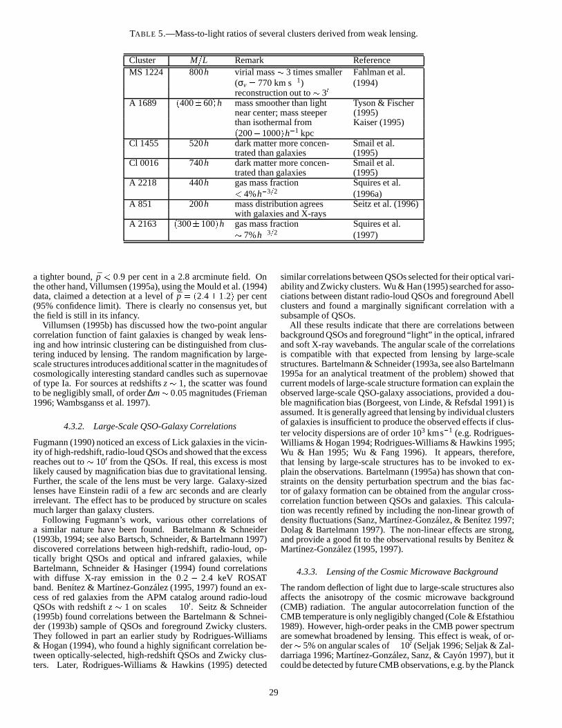
TABLE 5.—Mass-to-light ratios of several clusters derived from weak lensing.

Cluster M=L Remark ReferenceMS 1224 800h virial mass 3 times smaller Fahlman et al.

(σv = 770 km s1) (1994)reconstruction out to 30

A 1689 (40060)h mass smoother than light Tyson & Fischernear center; mass steeper (1995)than isothermal from Kaiser (1995)(2001000)h1 kpc

Cl 1455 520h dark matter more concen- Smail et al.trated than galaxies (1995)

Cl 0016 740h dark matter more concen- Smail et al.trated than galaxies (1995)

A 2218 440h gas mass fraction Squires et al.< 4%h3=2 (1996a)

A 851 200h mass distribution agrees Seitz et al. (1996)with galaxies and X-rays

A 2163 (300100)h gas mass fraction Squires et al. 7%h3=2 (1997)

a tighter bound, p < 0:9 per cent in a 2.8 arcminute field. Onthe other hand, Villumsen (1995a), using the Mould et al. (1994)data, claimed a detection at a level of p = (2:4 1:2) per cent(95% confidence limit). There is clearly no consensus yet, butthe field is still in its infancy.

Villumsen (1995b) has discussed how the two-point angularcorrelation function of faint galaxies is changed by weak lens-ing and how intrinsic clustering can be distinguished from clus-tering induced by lensing. The random magnification by large-scale structures introduces additional scatter in the magnitudes ofcosmologically interesting standard candles such as supernovaeof type Ia. For sources at redshifts z 1, the scatter was foundto be negligibly small, of order ∆m 0:05 magnitudes (Frieman1996; Wambsganss et al. 1997).

4.3.2. Large-Scale QSO-Galaxy Correlations

Fugmann (1990) noticed an excess of Lick galaxies in the vicin-ity of high-redshift, radio-loud QSOs and showed that the excessreaches out to 100 from the QSOs. If real, this excess is mostlikely caused by magnification bias due to gravitational lensing.Further, the scale of the lens must be very large. Galaxy-sizedlenses have Einstein radii of a few arc seconds and are clearlyirrelevant. The effect has to be produced by structure on scalesmuch larger than galaxy clusters.

Following Fugmann’s work, various other correlations ofa similar nature have been found. Bartelmann & Schneider(1993b, 1994; see also Bartsch, Schneider, & Bartelmann 1997)discovered correlations between high-redshift, radio-loud, op-tically bright QSOs and optical and infrared galaxies, whileBartelmann, Schneider & Hasinger (1994) found correlationswith diffuse X-ray emission in the 0:2 2:4 keV ROSATband. Benıtez & Martınez-Gonzalez (1995, 1997) found an ex-cess of red galaxies from the APM catalog around radio-loudQSOs with redshift z 1 on scales . 100. Seitz & Schneider(1995b) found correlations between the Bartelmann & Schnei-der (1993b) sample of QSOs and foreground Zwicky clusters.They followed in part an earlier study by Rodrigues-Williams& Hogan (1994), who found a highly significant correlation be-tween optically-selected, high-redshift QSOs and Zwicky clus-ters. Later, Rodrigues-Williams & Hawkins (1995) detected

similar correlations between QSOs selected for their optical vari-ability and Zwicky clusters. Wu & Han (1995) searched for asso-ciations between distant radio-loud QSOs and foreground Abellclusters and found a marginally significant correlation with asubsample of QSOs.

All these results indicate that there are correlations betweenbackground QSOs and foreground “light” in the optical, infraredand soft X-ray wavebands. The angular scale of the correlationsis compatible with that expected from lensing by large-scalestructures. Bartelmann & Schneider (1993a, see also Bartelmann1995a for an analytical treatment of the problem) showed thatcurrent models of large-scale structure formation can explain theobserved large-scale QSO-galaxy associations, provided a dou-ble magnification bias (Borgeest, von Linde, & Refsdal 1991) isassumed. It is generally agreed that lensing by individual clustersof galaxies is insufficient to produce the observed effects if clus-ter velocity dispersions are of order 103 kms1 (e.g. Rodrigues-Williams & Hogan 1994; Rodrigues-Williams & Hawkins 1995;Wu & Han 1995; Wu & Fang 1996). It appears, therefore,that lensing by large-scale structures has to be invoked to ex-plain the observations. Bartelmann (1995a) has shown that con-straints on the density perturbation spectrum and the bias fac-tor of galaxy formation can be obtained from the angular cross-correlation function between QSOs and galaxies. This calcula-tion was recently refined by including the non-linear growth ofdensity fluctuations (Sanz, Martınez-Gonzalez, & Benıtez 1997;Dolag & Bartelmann 1997). The non-linear effects are strong,and provide a good fit to the observational results by Benıtez &Martınez-Gonzalez (1995, 1997).

4.3.3. Lensing of the Cosmic Microwave Background

The random deflection of light due to large-scale structures alsoaffects the anisotropy of the cosmic microwave background(CMB) radiation. The angular autocorrelation function of theCMB temperature is only negligibly changed (Cole & Efstathiou1989). However, high-order peaks in the CMB power spectrumare somewhat broadened by lensing. This effect is weak, of or-der 5% on angular scales of. 100 (Seljak 1996; Seljak & Zal-darriaga 1996; Martınez-Gonzalez, Sanz, & Cayon 1997), but itcould be detected by future CMB observations, e.g. by the Planck

29

Microwave Satellite.

4.3.4. Outlook: Detecting Dark Matter Concentrations

If lensing is indeed responsible for the correlations discussedabove, other signatures of lensing should be found. Fort et al.(1996) searched for shear due to weak lensing in the fields offive luminous QSOs and found coherent signals in all five fields.In addition, they detected foreground galaxy groups for three ofthe sources. Earlier, Bonnet et al. (1993) had found evidence fora coherent shear pattern in the field of the lens candidate QSO2345+007. The shear was later identified with a distant cluster(Mellier et al. 1994; Fischer et al. 1994).

In general, it appears that looking for weak coherent imagedistortions provides an excellent way of searching for otherwiseinvisible dark matter concentrations. A systematic technique forthis purpose has been developed by Schneider (1996a). Weaklensing outside cluster fields may in the near future allow ob-servers to obtain samples of mass concentrations which are se-lected purely on the basis of their lensing effect. Such a selec-tion would be independent of the mass-to-light ratio, and wouldpermit the identification and study of nonlinear structures in theuniverse with unusually large mass-to-light ratios. This wouldbe complementary to the limits on compact masses discussed inSect. 2.3.2..

Acknowledgements

The authors thank Rosanne Di Stefano, Andreas Huss, Chris Ko-chanek, Tsafrir Kolatt, Shude Mao, Peter Schneider and UrosSeljak for helpful comments on the manuscript. This work wassupported in part by NSF grant AST 9423209 and by the Son-derforschungsbereich SFB 375-95 of the Deutsche Forschungs-gemeinschaft.

REFERENCES

Alard, C. 1995, in: Astrophysical Applications of Gravitational Lensing, Proc.IAU Symp. 173, eds. C.S. Kochanek & J.N. Hewitt (Boston: Kluwer)

Alard, C., Guibert, J. 1997, A&A, 326, 1Alard, C., Mao, S., Guibert, J. 1995, A&A, 300, L17Albrow, M., Beaulieu, J.-P., Birch, P. et al. 1996, in: Variable Stars and the As-

trophysical Returns of Microlensing Surveys, Proc. 12th IAP Conf., eds. R.Ferlet, J.-P. Maillard & B. Raban (Gif-Sur-Yvette: Editions Frontieres)

Alcock, C., Akerlof, C.W., Allsman, R.A. et al. 1993, Nat, 365, 621Alcock, C., Allsman, R., Axelrod, T. et al. 1995a, Phys. Rev. Lett., 74, 2867Alcock, C., Allsman, R.A., Alves, D. et al. 1995b, ApJ, 454, L125Alcock, C., Allsman, R.A., Axelrod, T.S. et al. 1996, ApJ, 461, 84Alcock, C., Allsman, R.A., Alves, D. et al. 1997, ApJ, 479, 119Ansari, R., Cavalier, F., Moniez, M. et al. 1996, A&A, 314, 94Aubourg, E., Bareyre, P., Brehin, P. et al. 1993, Nat, 365, 623Aubourg, E., Bareyre, P., Brehin, P. et al. 1995, A&A, 301, 1Babul, A., Lee, M.H. 1991, MNRAS, 250, 407Baillon, P., Bouquet, A., Giraud-Heraud, Y., Kaplan, J. 1993, A&A, 227, 1Bar-Kana, R. 1996, ApJ, 468, 17Bar-Kana, R. 1997, ApJ, 489, 21Bartelmann, M. 1995a, A&A, 298, 661Bartelmann, M. 1995b, A&A, 299, 11Bartelmann, M. 1995c, A&A, 303, 643Bartelmann, M. 1996, A&A, 313, 697Bartelmann, M., Narayan, R. 1995a, ApJ, 451, 60Bartelmann, M., Narayan, R. 1995b, in: Dark Matter, AIP Conf. Proc. 336, eds.

S.S. Holt & C.L. Bennett (New York: AIP Press)Bartelmann, M., Schneider, P. 1991, A&A, 248, 349Bartelmann, M., Schneider, P. 1993a, A&A, 268, 1Bartelmann, M., Schneider, P. 1993b, A&A, 271, 421Bartelmann, M., Schneider, P. 1994, A&A, 284, 1Bartelmann, M., Steinmetz, M. 1996, MNRAS, 283, 431

Bartelmann, M., Weiss, A. 1994, A&A, 287, 1Bartelmann, M., Ehlers, J., Schneider, P. 1993, A&A, 280, 351Bartelmann, M., Schneider, P., Hasinger, G. 1994, A&A, 290, 399Bartelmann, M., Steinmetz, M., Weiss, A. 1995, A&A, 297, 1Bartelmann, M., Narayan, R., Seitz, S., Schneider, P. 1996, ApJ, 464, L115Bartelmann, M., Huss, A., Colberg, J.M., Jenkins, A., Pearce, F.R. 1998, A&A,

330, 1Bartsch, A., Schneider, P., Bartelmann, M. 1997, A&A, 319, 375Benıtez, N., Martınez-Gonzalez, E. 1995, ApJ, 448, L89Benıtez, N., Martınez-Gonzalez, E. 1997, ApJ, 477, 27Bennett, D.P., Alcock, C., Allsman, R. et al. 1995, in: Dark Matter, AIP Conf.

Proc. 336, eds. S.S. Holt & C.L. Bennett (New York: AIP)Bergmann, A.G., Petrosian, V. 1993, ApJ, 413, 18Bergmann, A.G., Petrosian, V., Lynds, R. 1990, ApJ, 350, 23Bernardeau, F., Van Waerbeke, L., Mellier, Y. 1997, A&A, 322, 1Bernstein, G., Fischer, P., Tyson, J.A., Rhee, G. 1997, ApJ, 483, L79Bissantz, N., Englmaier, P., Binney, J., Gerhard, O. 1997, MNRAS, 289, 651Blaes, O.M., Webster, R.L. 1992, ApJ, 391, L63Blandford, R.D., Kochanek, C.S. 1987, ApJ, 321, 658Blandford, R.D., Kochanek, C.S., Kovner, I., Narayan, R. 1989, Science, 245,

824Blandford, R.D., Narayan, R. 1986, ApJ, 310, 568Blandford, R.D., Narayan, R. 1992, ARA&A, 30, 311Blandford, R.D., Saust, A.B., Brainerd, T.G., Villumsen, J.V. 1991, MNRAS,

251, 600Bonnet, H., Mellier, Y. 1995, A&A, 303, 331Bonnet, H., Mellier, Y., Fort, B. 1994, ApJ, 427, L83Bonnet, H., Fort, B., Kneib, J.-P., Soucail, G., Mellier, Y. 1993, A&A, 289, L7Borgeest, U., von Linde, J., Refsdal, S. 1991, A&A, 251, L35Brainerd, T.G., Blandford, R.D., Smail, I. 1996, ApJ, 466, 623Broadhurst, T. 1995, in: Dark Matter, AIP Conf. Proc. 336, eds. S.S. Holt & C.L.

Bennett (New York: AIP)Broadhurst, T., Taylor, A., Peacock, J. 1995, ApJ, 438, 49Buchalter, A., Kamionkowski, M., Rich, R.M. 1996, ApJ, 469, 676Burke, W.L. 1981, ApJ, 244, L1Canizares, C.R. 1982, ApJ, 263, 508Carlberg, R.G. 1994, ApJ, 433, 468Carlberg, R.G., Yee, H.K.C., Ellingson, E. 1994, ApJ, 437, 63Carr, B. 1994, ARA&A, 32, 531Cen, R.Y., Gott III, J.R., Ostriker, J.P., Turner, E.L. 1994, ApJ, 423, 1Chang, K., Refsdal, S. 1979, Nat, 282, 561Chwolson, O. 1924, Astron. Nachr., 221, 329Cole, S., Efstahiou, G. 1989, MNRAS, 239, 195Colley, W.N. 1995, AJ, 109, 440Corbett, E.A., Browne, I.W.A., Wilkinson, P.N., Patnaik, A.R. 1996, in: Astro-

physical Applications of Gravitational Lensing, Proc. IAU Symp. 173, eds.C.S. Kochanek & J.N. Hewitt (Boston: Kluwer)

Corrigan, R.T., Irwin, M.J., Arnaud, J., Fahlman, G.G., Fletcher, J.M. et al. 1991,AJ, 102, 34

Courbin, F., Magain, P., Keeton, C.R., Kochanek, C.S., Vanderriest, C., Jaunsen,A.O., Hjorth, J. 1997, A&A, 324, L1

Crone, M.M., Evrard, A.E., Richstone, D.O. 1996, 1996, ApJ, 467, 489Crotts, A.P.S. 1992, ApJ, 399, L43Crotts, A.P.S., Tomaney, A.B. 1996, ApJ, 473, L87Daines, S., Jones, C., Forman, W., Tyson, A. 1996, preprintDalcanton, J.J., Canizares, C.R., Granados, A., Steidel, C.C., Stocke, J.T. 1994,

ApJ, 424, 550Dell’Antonio, I.P., Tyson, J.A. 1996, ApJ, 473, L17De Rujula, A., Jetzer, P., Masso, E. 1991, MNRAS, 250, 348Di Stefano, R., Esin, A.A. 1995, ApJ, 448, L1Di Stefano, R., Mao, S. 1996, ApJ, 457, 93Dolag, K., Bartelmann, M. 1997, MNRAS, 291, 446Durret, F., Gerbal, D., Lachieze-Rey, M., Lima-Neto, G., Sadat, R. 1994, A&A,

287, 733Dyson, F.W., Eddington, A.S., & Davidson, C.R. 1920, Mem. R. Astron. Soc.,

62, 291Eddington, A.S. 1920, Space, Time and Gravitation (Cambridge: University

Press)Einstein, A. 1911, Annalen der Physik, 35, 898Einstein, A. 1915, Sitzungsber. Preuß. Akad. Wissensch., erster Halbband, p. 831Einstein, A. 1936, Sci, 84, 506

30

Erdl, H., Schneider, P. 1992, A&A, 268, 453Fahlman, G., Kaiser, N., Squires, G., Woods, D. 1994, ApJ, 437, 56Falco, E.E., Gorenstein, M.V., Shapiro, I.I. 1985, ApJ, 289, L1Falco, E.E., Gorenstein, M.V., Shapiro, I.I. 1991, ApJ, 372, 364Falco, E.E., Kochanek, C.S., Munoz, J.A. 1998, ApJ, 494, 47Falco, E.E., Shapiro, I.I., Moustakas, L.A., Davis, M. 1997, ApJ, submittedFischer, P., Tyson, J.A., Bernstein, G.M., Guhathakurta, P. 1994, ApJ, 431, L71Fischer, P., Bernstein, G., Rhee, G., Tyson, J.A. 1997, AJ, 113, 521Flores, R., Primack, J. 1996, ApJ, 457, L5Fort, B., Mellier, Y. 1994, A&AR, 5, 239Fort, B., Prieur, J.L., Mathez, G., Mellier, Y., Soucail, G. 1988, A&A, 200, L17Fort, B., Le Fevre, O., Hammer, F., Cailloux, M. 1992, ApJ, 399, L125Fort, B., Mellier, Y., Dantel-Fort, M., Bonnet, H., Kneib, J.-P. 1996, A&A, 310,

705Frieman, J. 1996, Comments on Astrophysics, in press; preprint astro-

ph/9608068Fugmann, W. 1990, A&A, 240, 11Fukugita, M., Turner, E.L. 1991, MNRAS, 253, 99Fukugita, M., Futamase, T., Kasai, M., Turner, E.L. 1992, ApJ, 393, 3Garrett, M.A., Calder, R.J., Porcas, R.W., King, L.J., Walsh, D., Wilkinson, P.N.

1994, MNRAS, 270, 457Gerbal, D., Durret, F., Lima-Neto, G., Lachieze-Rey, M. 1992, A&A, 253, 77Gondolo, P., Ansari, R., Auriere, M. et al. 1997, in: Dark and Visible Matter in

Galaxies, Proc. Conf. Sesto Pusteria, Italy, eds. M. Persic & P. Salucci (SanFrancisco: ASP)

Gorenstein, M.V., Cohen, N.L., Shapiro, I.I., Rogers, A.E.E., Bonometti, R.J.,Falco, E.E., Bartel, N., Marcaide, J.M. 1988, ApJ, 334, 42

Gott, J.R. 1981, ApJ, 243, 140Gould, A. 1992a, ApJ, 386, L5Gould, A. 1992b, ApJ, 392, 442Gould, A. 1994a, ApJ, 421, L71Gould, A. 1994b, ApJ, 421, L75Gould, A. 1996, ApJ, 470, 201Gould, A., Loeb, A. 1992, ApJ, 396, 104Griest, K. 1991, ApJ, 366, 412Griest, K., Hu, W. 1992, ApJ, 397, 362Griest, K., Alcock, C., Axelrod, T.S. 1991, ApJ, 372, L79Griffiths, R.E., Casertano, S., Im, M., Ratnatunga, K.U. 1996, MNRAS, 282,

1159Grogin, N., & Narayan, R. 1996, ApJ, 464, 92Grossman, S.A., Narayan, R. 1988, ApJ, 324, L37Grossman, S.A., Narayan, R. 1989, ApJ, 344, 637Grossman, S.A., Saha, P. 1994, ApJ, 431, 74Gunn, J.E. 1967, ApJ, 150, 737Hammer, F. 1991, ApJ, 383, 66Hammer, F., Rigaut, F. 1989, A&A, 226, 45Henstock, D.R., Browne, I.W.A., Wilkinson, P.N., Taylor, G.B., Vermeulen,

R.C., Pearson, T.J., Readhead, R.C.S. 1995, ApJS, 100, 1Haarsma, D.B., Hewitt, J.N., Burke, B.F., Lehar, J. 1996, in: Astrophysical Ap-

plications of Gravitational Lensing, IAU Symp. 173, eds. C.S. Kochanek &J.N. Hewitt (Boston: Kluwer)

Haarsma, D.B., Hewitt, J.N., Lehar, J., Burke, B.F. 1997, ApJ, 479, 102Hewitt, J.N., Turner, E.L., Lawrence, C.R., Schneider, D.P., Gunn, J.E. et al.

1987, ApJ, 321, 706Huchra, J., Gorenstein, M., Kent, S., Shapiro, I., Smith, G. et al. 1985, AJ, 90,

691Im, M., Griffiths, R.E., Ratnatunga, K. 1997, ApJ, 475, 457Irwin, M.J., Webster, R.L., Hewett, P.C., Corrigan, R.T., Jedrzejewski, R.I. 1989,

AJ, 98, 1989Jain, B., Seljak, U. 1997, ApJ, 484, 560Jaroszynski, M., Park, C., Paczynski, B., Gott, J.R. 1990, ApJ, 365, 22Jetzer, P. 1994, A&A, 286, 426Kaiser, N. 1992, ApJ, 388, 272Kaiser, N. 1995, ApJ, 439, L1Kaiser, N. 1996, ApJ, submitted; preprint astro-ph/9610120Kaiser, N., Squires, G. 1993, ApJ, 404, 441Kaiser, N., Squires, G., Broadhurst, T. 1995, ApJ, 449, 460Kaiser, N., Squires, G., Fahlman, G., Woods, D., Broadhurst, T. 1995, in: Proc.

35th Herstmonceux Conf., ed. S. Maddox (Singapore: World Scientific)Kamionkowski, M. 1995, ApJ, 442, L9Kassiola, A., Kovner, I. 1993, ApJ, 417, 450

Kassiola, A., Kovner, I., Blandford, R.D. 1991, ApJ, 381, 6Kassiola, A., Kovner, I., Blandford, R.D. 1992, ApJ, 396, 10Keeton II, C.R., Kochanek, C.S. 1996, in: Astrophysical Applications of Gravi-

tational Lensing, IAU Symp. 173, eds. C.S. Kochanek & J.N. Hewitt (Boston:Kluwer)

Keeton II, C.R., Kochanek, C.S. 1997, ApJ, 487, 42Keeton II, C.R., Kochanek, C.S. 1998, ApJ, 495, 157Keeton II, C.R., Kochanek, C.S., Seljak, U. 1997, ApJ, 482, 604Kiraga, M., Paczynski, B. 1994, ApJ, 430, L101Kneib, J.-P., Ellis, R.S., Smail, I., Couch, W.T., Sharples, R.M. 1996, ApJ, 471,

643Kneib, J.-P., Mellier, Y., Fort, B., Mathez, G. 1993, A&A, 273, 367Kochanek, C.S. 1990, MNRAS, 247, 135Kochanek, C.S. 1991, ApJ, 373, 354Kochanek, C.S. 1992, ApJ, 384, 1Kochanek, C.S. 1993a, ApJ, 417, 438Kochanek, C.S. 1993b, ApJ, 419, 12Kochanek, C.S. 1995a, ApJ, 445, 559Kochanek, C.S. 1995b, ApJ, 453, 545Kochanek, C.S. 1996a, ApJ, 466, 638Kochanek, C.S. 1996b, ApJ, 473, 595Kochanek, C.S., Narayan, R. 1992, ApJ, 401, 461Kochanek, C.S., Blandford, R.D., Lawrence, C.R., Narayan, R. 1989, MNRAS,

238, 43Kovner, I. 1987, ApJ, 312, 22Kovner, I. 1989, ApJ, 337, 621Kristian, J., Sachs, R.K. 1966, ApJ, 143, 379Kundic, T., Turner, E.L., Colley, W.N. et al. 1996, astro-ph/9610162Lacey, C., Cole, S. 1993, MNRAS, 262, 627Lacey, C., Cole, S. 1994, MNRAS, 271, 676Le Fevre, O., Hammer, F., Angonin-Willaime, M.-C., Gioia, I.M., Luppino, G.A.

1994, ApJ, 422, L5Lehar, J., Hewitt, J.N., Roberts, D.H., Burke, B.F. 1992, ApJ, 384, 453Loeb, A., Mao, S. 1994, ApJ, 435, L109Luppino, G.A., Gioia, I.M., Annis, J., Le Fevre, O., Hammer, F. 1993, ApJ,, 416,

444Luppino, G.A., Kaiser, N. 1997, ApJ, 475, 20Lynds, R., Petrosian, V. 1986, BAAS, 18, 1014Malhotra, S., Rhoads, J.E., Turner, E.L. 1997, MNRAS, 288, 138Maller, A.H., Flores, R.A., Primack, J.R. 1997, ApJ, 486, 681Mao, S., Paczynski, B. 1991, ApJ, 374, L37Mao, S., Kochanek, C.S. 1994, MNRAS, 268, 569Mao, S., Paczynski, B. 1996, ApJ, 473, 57Maoz, D., Rix, H.-W. 1993, ApJ, 416, 425Maoz, D., Rix, H.-W., Gal-Yam, A., Gould, A. 1997, ApJ, 486, 75Martınez-Gonzalez, E., Sanz, J.L., Cayon, L. 1997, ApJ, 484, 1Mathez, G., Fort, B., Mellier, Y., Picat, J.-P., Soucail, G. 1992, A&A, 256, 343Mellier, Y., Fort, B., Kneib, J.-P. 1993, ApJ, 407, 33Mellier, Y., Dantel-Fort, M., Fort, B., Bonnet, H. 1994, A&A, 289, L15Miralda-Escude, J. 1991a, ApJ, 370, 1Miralda-Escude, J. 1991b, ApJ, 380, 1Miralda-Escude, J. 1992, ApJ, 390, L65Miralda-Escude, J. 1993, ApJ, 403, 497Miralda-Escude, J. 1995, ApJ, 438, 514Miralda-Escude, J., Babul, A. 1995, ApJ, 449, 18Mohr, J.J., Evrard, A.E., Fabricant, D.G., Geller, M.J. 1995, ApJ, 447, 8Mould, J., Blandford, R.D., Villumsen, J.V., Brainerd, T.G., Smail, I., Small, T.,

Kells, W. 1994, MNRAS, 271, 31Myers, S.T., Fassnacht, C.D., Djorgovski, S.G., Blandford, R.D., et al. 1995,

ApJ, 447, L5Narayan, R. 1991, ApJ, 378, L5Narayan, R., Grossman, S. 1989, in: Gravitational Lenses, eds. J.M. Moran, J.N.

Hewitt, K.Y. Lo (Berlin: Springer-Verlag)Narayan, R., White, S.D.M. 1988, MNRAS, 231, 97PNarayan, R., Wallington, S. 1993, in: Gravitational Lenses in the Universe, Proc.

31stLiege Astroph. Coll., eds. J. Surdej et al.Narayan, R., Blandford, R.D., Nityananda, R. 1984, Nat, 310, 112Natarajan, P., Kneib, J.-P. 1996, MNRAS, 283, 1031Navarro, J.F., Frenk, C.S., White, S.D.M. 1996, ApJ, 462, 563Nemiroff, R.J., Wickramasinghe, W.A.D.T. 1994, ApJ, 424, L21

31

Nemiroff, R.J., Norris, J.P., Wickramasinghe, W.A.D.T., Horack, J.M., Kouve-liotou, C. et al. 1993, ApJ, 414, 36

Nemiroff, R.J., Wickramasinghe, W.A.D.T., Norris, J.P., Kouveliotou, C., Fish-man, G.J. et al. 1994, ApJ, 432, 478

Nityananda, R., Samuel, J. 1992, Phys. Rev. D, 45, 3862Østensen, R., Refsdal, S., Stabell, R., Teuber, J., Emanuelsen, P.I. et al.: 1996,

A&A, 309, 59Paczynski, B. 1986a, ApJ, 301, 503Paczynski, B. 1986b, ApJ, 304, 1Paczynski, B. 1987, Nat, 325, 572Paczynski, B. 1991, ApJ, 371, L63Paczynski, B. 1996, ARA&A, 34, 419Paczynski, B., Stanek, K.Z., Udalski, A., Szymanski, M., Kałuzny, J., Kubiak,

M., Mateo, M., Krzeminski, W. 1994, ApJ, 435, L113Pello-Descayre, R., Soucail, G., Sanahuja, B., Mathez, G., Ojero, E. 1988, A&A,

190, L11Pello, R., Le Borgne, J.F., Soucail, G., Mellier, Y., Sanahuja, B. 1991, ApJ, 366,

405Pelt, J., Hoff, W., Kayser, R., Refsdal, S., Schramm, T. 1994, A&A, 286, 775Pelt, J., Kayser, R., Refsdal, S., Schramm, T. 1996, A&A, 305, 97Pierre, M., Le Borgne, J.F., Soucail, G., Kneib, J.P. 1996, A&A, 311, 413Pratt, M. 1996, in: Microlensing, Proc. 2nd International Workshop on Gravita-

tional Microlensing Surveys, Orsay, France; ed. M. MoniezPress, W.H., Gunn, J.E. 1973, ApJ, 185, 397Press, W.H., Rybicki, G.B., Hewitt, J.N. 1992a, ApJ, 385, 404Press, W.H., Rybicki, G.B., Hewitt, J.N. 1992b, ApJ, 385, 416Rauch, K.P., Blandford, R.D. 1991, ApJ, 381, L39Refsdal, S. 1964, MNRAS, 128, 307Refsdal, S. 1966a, MNRAS, 132, 101Refsdal, S. 1966b, MNRAS, 134, 315Refsdal, S., Surdej, J. 1994, Rep. Progr. Phys., 57, 117

Renault, C., Afonso, C., Aubourg, E., Bareyre, P. et al. 1997, A&A, 324, L69Richstone, D.O., Loeb, A., Turner, E.L. 1992, ApJ, 393, 477Rix, H.-W., Maoz, D., Turner, E.L., Fukugita, M. 1994, ApJ, 435, 49Rodrigues-Williams, L.L., Hogan, C.J. 1994, AJ, 107, 451Rodrigues-Williams, L.L., Hawkins, M.R.S. 1995, in: Dark Matter, AIP Conf.

Proc. 336, eds. S.S. Holt & C.L. Bennett (New York: AIP)Roulet, E., Mollerach, S. 1997, Phys. Reports, 279, 67Sackett, P.D. 1996, in: Microlensing, Proc. 2nd International Workshop on Grav-

itational Microlensing Surveys, Orsay, France; ed. M. MoniezSahu, K.C. 1994, Nat, 370, 275Sahu, K.C. 1996, in: Microlensing, Proc. 2nd International Workshop on Gravi-

tational Microlensing Surveys, Orsay, France; ed. M. MoniezSanz, J.L., Martınez-Gonzalez, E., Benıtez, N. 1997, MNRAS, 291, 418Schechter, P.L., Bailyn, C.D., Barr, R. et al. 1997, ApJ, 475, L85Schild, R.E., Smith, R.C. 1991, AJ, 101, 813Schild, R.E., Thomson, D.J. 1993, in: Gravitational Lenses in the Universe,

Proc. 31st Liege Int. Astroph. Coll., eds. J. Surdej et al.Schmidt, M. 1963, Nat, 197, 1040Schneider, P. 1985, A&A, 143, 413Schneider, P. 1993, A&A, 279, 1Schneider, P. 1995, A&A, 302, 639Schneider, P. 1996a, MNRAS, 283, 837Schneider, P. 1996b, in: Cosmological Applications of Gravitational Lensing,

in: The universe at high-z, large-scale structure and the cosmic microwavebackground, Lecture Notes in Physics, eds. E. Martınez-Gonzalez & J.L. Sanz(Berlin: Springer Verlag)

Schneider, P., Bartelmann, M. 1997, MNRAS, 286, 696Schneider, P., Seitz, C. 1995, A&A, 294, 411Schneider, P., Weiss, A. 1987, A&A, 171, 49Schneider, P., Ehlers, J., Falco, E.E. 1992, Gravitational Lenses (Berlin:

Springer Verlag)Seitz, C., Schneider, P. 1995a, A&A, 297, 287Seitz, C., Wambsganss, J., Schneider, P. 1994, A&A, 288, 19Seitz, C., Kneib, J.-P., Schneider, P., Seitz, S. 1996, A&A, 314, 707Seitz, S., Schneider, P. 1995b, A&A, 302, 9Seitz, S., Schneider, P. 1996, A&A, 305, 383Seljak, U. 1994, ApJ, 436, 509Seljak, U. 1996, ApJ, 463, 1Seljak, U., Zaldarriaga, M. 1996, ApJ, 469, 437Shapiro, I.I. 1964, Phys. Rev. Lett., 13, 789

Smail, I., Dickinson, M. 1995, ApJ, 455, L99Smail, I., Ellis, R.S., Fitchett, M.J., Edge, A.C. 1995, MNRAS, 273, 277Smail, I., Ellis, R.S., Fitchett, M.J., Norgaard-Nielsen, H.U., Hansen, L., Jor-

gensen, H.J. 1991, MNRAS, 252, 19Smail, I., Dressler, A., Kneib, J.-P., Ellis, R.S., Couch, W.J., Sharples, R.M.,

Oemler Jr., A. 1996, ApJ, 469, 508Smail, I., Ellis, R.S., Dressler, A., Couch, W.J., Oemler Jr., A., Sharples, R.M.,

Butcher, H. 1997, ApJ, 479, 70Soldner, J. 1804, Berliner Astron. Jahrb. 1804, p. 161Soucail, G., Fort, B., Mellier, Y., Picat, J.P. 1987a, A&A, 172, L14Soucail, G., Mellier, Y., Fort, B., Hammer, F., Mathez, G. 1987b, A&A, 184, L7Squires, G., Kaiser, N., Babul, A., Fahlman, G., Woods, D., Neumann, D.,

Bohringer, H. 1996a, ApJ, 461, 572Squires, G., Kaiser, N., Fahlman, G., Babul, A., Woods, D., 1996b, ApJ, 469, 73Squires, G., Neumann, D.M., Kaiser, N., Arnaud, M., Babul, A., Bohringer, H.,

Fahlman, G., Woods, D. 1997, ApJ, 482, 648Stanek, K.Z., Paczynski, B., Goodman, J. 1993, ApJ, 413, L7Subramanian, K., Cowling, S.A. 1986, MNRAS, 219, 333Surdej, J., Claeskens, J.-F., Crampton, D., Filippenko, A.V., Hutsemekers, D. et

al. 1993, AJ, 105, 2064Surpi, G.C., Harari, D.D., Frieman, J.A. 1996, ApJ, 464, 54Sutherland, W., Alcock, C., Allsman, R.A. et al. 1996, in: Proc. Workshop

on Identification of Dark Matter, Sheffield, 1996, in press; preprint astro-ph/9611059

Turner, E.L. 1980, ApJ, 242, L135Turner, E.L. 1990, ApJ, 365, L43Turner, E.L., Ostriker, J.P., Gott, J.R. 1984, ApJ, 284, 1Tyson, J.A. 1988, AJ, 96, 1Tyson, J.A. 1990, Gravitational Lensing, Proc. Workshop Toulouse 1989 (Berlin:

Springer)Tyson, J.A. 1995, in: Dark Matter, AIP Conf. Proc 336, eds. S.S. Holt & C.L.

Bennett (New York: AIP)Tyson, J.A., Valdes, F., Wenk, R.A. 1990, ApJ, 349, L1Tyson, J.A., Fischer, P. 1995, ApJ, 446, L55Udalski, A., Szymanski, M., Kałuzny, J., Kubiak, M., Mateo, M. 1992, Acta As-

tron., 42, 253Udalski, A., Szymanski, M., Kałuzny, J., Kubiak, M., Krzeminski, W. et al. 1993,

Acta Astron. 43, 289Udalski, A., Szymanski, M., Mao, S., Di Stefano, R., Kałuzny, J., Kubiak, M.,

Mateo, M., Krzeminski, W. 1994, ApJ, 436, L103Vanderriest, C., Schneider, J., Herpe, G., Chevreton, M., Moles, M., Wlerick, G.

1989, A&A, 215, 1Villumsen, J.V. 1995a, MNRAS, submitted; preprint astro-ph/9507007Villumsen, J.V. 1995b, MNRAS, submitted; preprint astro-ph/9512001Villumsen, J.V. 1996, MNRAS, 281, 369Walsh, D., Carswell, R.F., & Weymann, R.J. 1979, Nat, 279, 381Wallington, S., Narayan, R. 1993, ApJ, 403, 517Wallington, S., Kochanek, C.S., Koo, D.C. 1995, ApJ, 441, 58Wallington, S., Kochanek, C.S., Narayan, R. 1996, ApJ, 465, 64Wallington, S., Narayan, R., Kochanek, C.S. 1994, ApJ, 426, 60Wambsganss, J. 1990, Ph.D. Thesis, MPA report #550Wambsganss, J., Paczynski, B., Schneider, P. 1990, ApJ, 358, L33Wambsganss, J., Cen, R.Y., Ostriker, J.P. 1998, ApJ, 494, 29Wambsganss, J., Cen, R.Y., Ostriker, J.P., Turner, E.L. 1995, Sci, 268, 274Wambsganss, J., Cen, R., Xu, G., Ostriker, J.P. 1997, ApJ, 475, L81Wang, Y., Turner, E.L. 1997, MNRAS, 292, 863Webster, R.L., Ferguson, A.M.N., Corrigan, R.T., Irwin, M.J. 1991, AJ, 102,

1939Wilson, G., Cole, S., Frenk, C.S. 1996, MNRAS, 282, 501Witt, H.J. 1993, ApJ, 403, 530Witt, H.J. 1995, ApJ, 449, 42Witt, H.J., Mao, S. 1994, ApJ, 430, 505Wu, X.-P. 1996, Fund. Cosmic Phys., 17, 1Wu, X.-P., Hammer, F. 1993, MNRAS, 262, 187Wu, X.-P., Han, J. 1995, MNRAS, 272, 705Wu, X.-P., Fang, L.-Z. 1996, ApJ, 461, L5Zhao, H.S., Mao, S. 1996, MNRAS, 283, 1197Zhao, H.S., Spergel, D.N., Rich, R.M. 1995, ApJ, 440, L13Zhao, H.S., Rich, R.M., Spergel, D.N. 1996, MNRAS, 282, 175Zwicky, F. 1937a, Phys. Rev. Lett., 51, 290Zwicky, F. 1937b, Phys. Rev. Lett., 51, 679

32