Astrophysical applications of gravitational microlensing

By Shude Mao

Ziang Yan Department of Physics ,Tsinghua

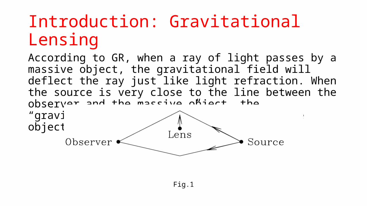
Introduction: Gravitational Lensing

According to GR, when a ray of light passes by a massive object, the gravitational field will deflect the ray just like light refraction. When the source is very close to the line between the observer and the massive object, the “gravitational refraction” make the massive object act like a “lens”.

Fig.1

Introduction: Phenomenon of GL

Fig.2 Cover of Gravitational Lensing:Strong, Weak and Micro

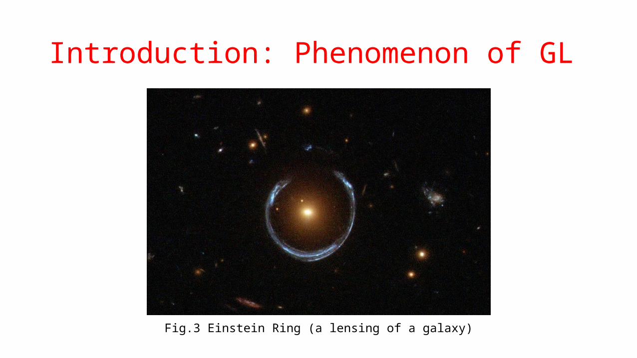
Introduction: Phenomenon of GL

Fig.3 Einstein Ring (a lensing of a galaxy)

Introduction: Phenomenon of GL

Fig.4 lensing by several galaxies

Introduction:Category of GL

• Microlensing by stars(GM)

• Multiple-images by galaxies

• Giant arcs and large-separation lenses by clusters of galaxies

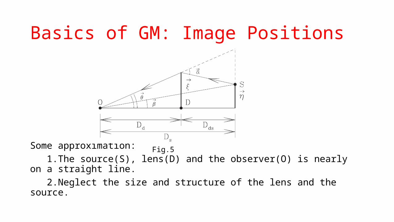
Basics of GM: Image Positions

Some approximation: 1.The source(S), lens(D) and the observer(O) is nearly on a straight line. 2.Neglect the size and structure of the lens and the source.

Fig.5

Basics of GM: Image PositionsLens equation: (1)The deflection angle is given by:

(2)

And the value of the scaled deflection angle is

(3)

where we have defined the angular Einstein radius as

(4) is the Einstein radius.when η=0, is the angle between the image and the object and the image will form the Einstein Ring

𝛽+𝛼=𝜃�̂�

𝑟 𝐸

Fig.5

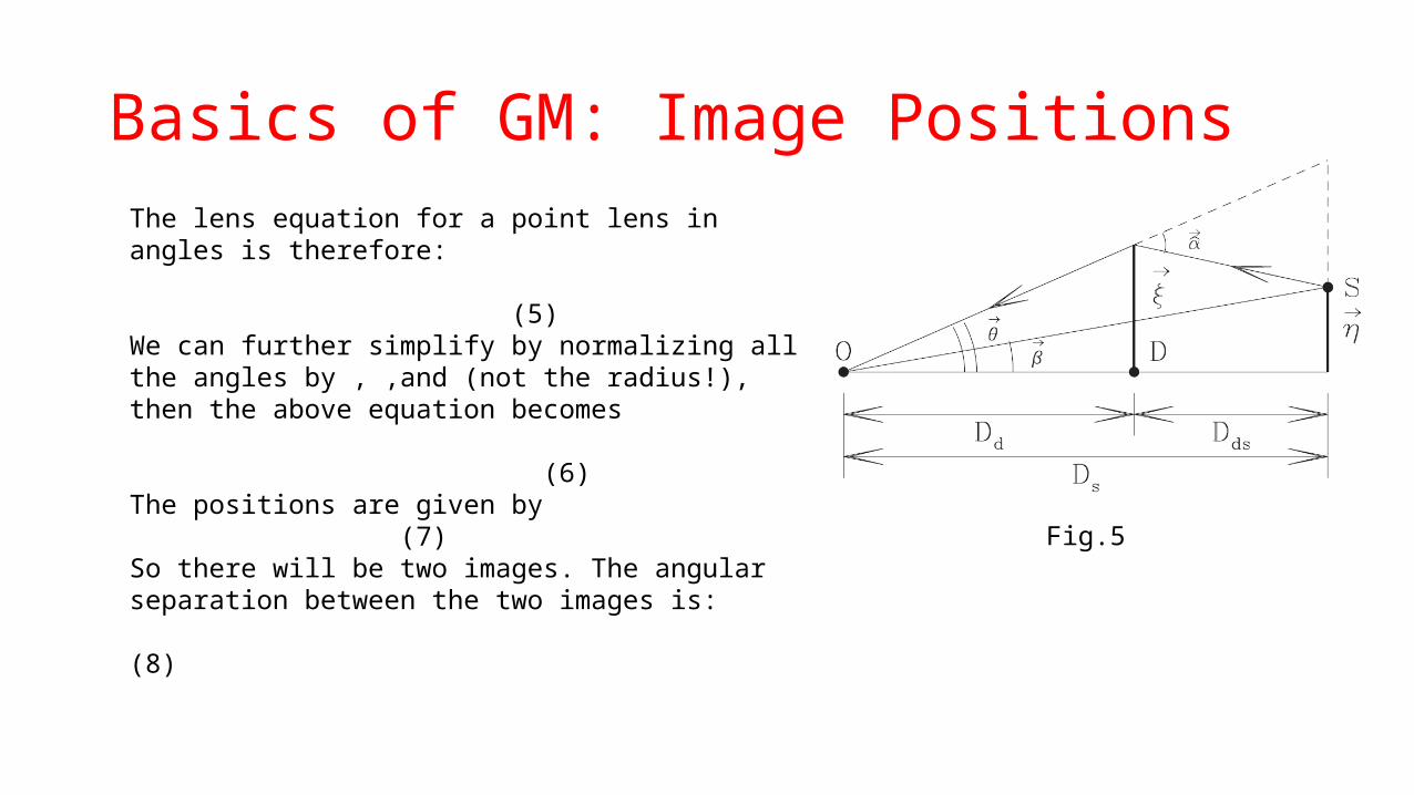
Basics of GM: Image PositionsThe lens equation for a point lens in angles is therefore: (5)We can further simplify by normalizing all the angles by , ,and (not the radius!), then the above equation becomes (6)The positions are given by (7)So there will be two images. The angular separation between the two images is: (8)

Fig.5

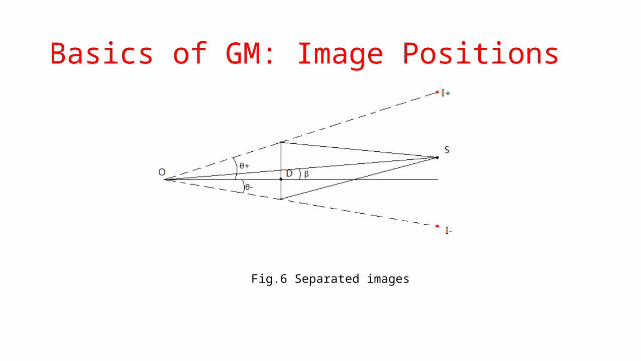
Basics of GM: Image Positions

Fig.6 Separated images

Basics of GM: Magnifications

Since gravitational lensing conserves surface brightness, the magnification of an image is simply given by the ratio of the image area and source area.For the source given by Fig.7,the magnifications can be given as: = (9)For two images given in (7),we find: (10) The total magnification is given by (11)

Fig.7

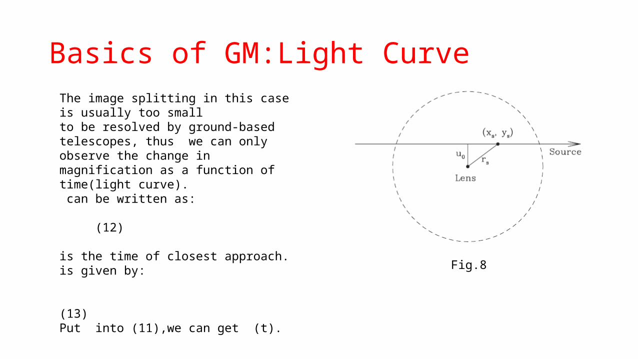
Basics of GM:Light CurveThe image splitting in this case is usually too smallto be resolved by ground-based telescopes, thus we can only observe the change in magnification as a function of time(light curve). can be written as: (12)

is the time of closest approach.is given by: (13)Put into (11),we can get (t).

Fig.8

Basics of GM: Light Curve

Fig.8 Light curve of a lensing event

Basics of GM: Degeneracy and Non-standard models• Degeneracy:Since depends on the lens mass, distances to the lensand source,

and the transverse velocity from an observed light curve well fitted by the standard model, one cannot uniquely infer the lens distance and mass. • Non-standard models: (1)Binary lens events: offers an exiting way to discover extrasolar planets (2)Binary source events: linear superposition of two sources (3)Finite source size events (4)Parallax/xallarap: parallax: The effect due to Earth’s motion around the xallarap: that due to binary motion in the source (5)Repeating events

Basics of GM:N-point Lens GM Write the lens equation in vector form:

, (14)

is the position(normalized by Einstein radius) of lenses with mass .

(14)can be solved use a complex form(see Witt(1990)):

= (15)

Where z=x+yi

In the complex form, the magnification is:

, (16)

From (15),we have

= (17)

So

(18)

Basics of GM: Critical Curves and Caustic

When J=0 in (16), the magnification will turn to infinity(in fact because of the finite size of the source and lens the magnification just have a sharp peak).The image position satisfying J=0 forms critical curves, which are mapped into caustics in the source plane.

Basics of GM: Critical Curves and Caustic

Fig.9 Critical curves and caustic in a binary system

Basics of GM: Optical Depth and Event RatesAs about 2000 unique microlensing events a observed, we need some statistical quantities to describe microlensing experiments. Now I’ll mention two of them.Optical Depth: the probability that a given source falls into the Einstein radius of any lensing star along the line of sight. (18)stands for the number density of lenses.The optical depth generally independent with mass M.

Basics of GM: Optical Depth and Event RatesEvent Rates: the probability of a given star that is within the Einstein radii of the lenses at any given instant.The probability of a source becoming a new microlensing event is: (19)Given the total number of sources (), the event rate is given by = (20)The event rate depends on M, so the timescale distribution can be used to probe the mass function of lenses in the Milky Way.

Applications of GM

1.Detect the main composition in the galactic halo. From the detections of MACHOs by microlensing, it is concluded that only ≤2%of the halo could be MACHOs. While earlier research 20%.2.Detect the galactic structure. With analyzing the optical depth and event rate.3.Analyze the stellar atmosphere and bulge formation Microlensing can magnify the signal-to-noise ratio.4.Detect exoplanets

Applications of GM: Detect Exoplanets

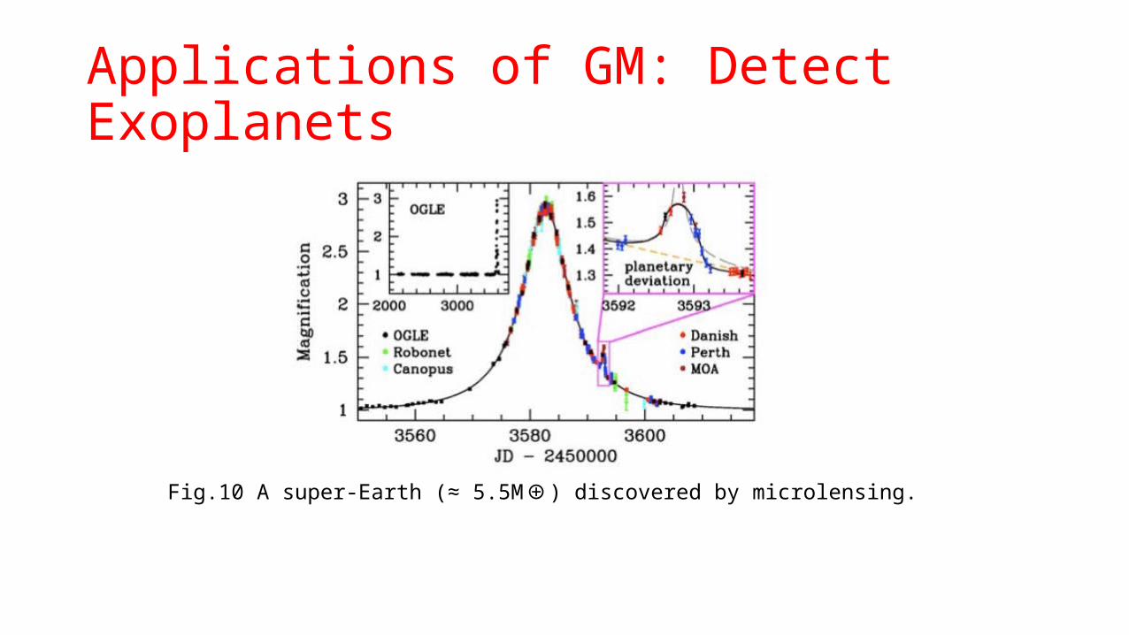
Fig.10 A super-Earth (≈ 5.5M ) discovered by microlensing.⊕

Applications of GM: Detecting Exoplanets

Fig.11 The first two-planet system discovered by Gaudi et al.

Applications of GM: Detecting Exoplanets

Fig.12 Extrasolar planets in the plane of mass vs. separation (in units of the snow line, indicated bythe vertical dashed green line). The red filled circles with error bars indicate planets found by microlensing.The black triangles and blue squares indicate the planetsdiscovered by radial velocities and transits, respectively. The magenta and green triangles indicatethe planets detected via direct imaging and timing, respectively.

Future of GM

• There are still much problems unsolved in the calculation of GM. e.g. The degenerate in the parallax events; how to distinguish exoplanet system with binary system; the number of critical curves and image numbers in a topological sense.• There are more and more collaborations participate in the detection

of GM like OGLE, MOA, SKYMAPPER and so on. Chinese scientists also make their distributions.

Thank you for listening!