Lecture Notes Methods of Mathematical Physics …iavramid/notes/appliedfunanal.pdfLecture Notes...
78
Lecture Notes Methods of Mathematical Physics MATH 536 Instructor: Ivan Avramidi Textbook: L. Debnath and P. Mikusinski, (Academic Press, 1999) New Mexico Institute of Mining and Technology Socorro, NM 87801 February 12, 2005 Author: Ivan Avramidi; File: appliedfunanal.tex; Date: May 24, 2005; Time: 13:58
Transcript of Lecture Notes Methods of Mathematical Physics …iavramid/notes/appliedfunanal.pdfLecture Notes...
Lecture NotesMethods of Mathematical Physics
MATH 536
Instructor: Ivan Avramidi
Textbook: L. Debnath and P. Mikusinski, (Academic Press, 1999)
New Mexico Institute of Mining and Technology
Socorro, NM 87801
February 12, 2005
Author: Ivan Avramidi; File: appliedfunanal.tex; Date:May 24, 2005; Time: 13:58
Contents
1 Integral Operators 31.1 Existense Theorems . . . . . . . . . . . . . . . . . . . . . . . . . 3
1.1.1 Integral Equations . . . . . . . . . . . . . . . . . . . . . 31.1.2 Neumann Series and Fredholm Alternative . . . . . . . . 41.1.3 Homework . . . . . . . . . . . . . . . . . . . . . . . . . 8
1.2 Fredholm Integral Equations . . . . . . . . . . . . . . . . . . . . 91.2.1 Hilbert-Schmidt and Trace -Class Operators . . . . . . . . 91.2.2 Linear Fredholm Equations . . . . . . . . . . . . . . . . . 111.2.3 Nonlinear Fredholm Equations . . . . . . . . . . . . . . . 131.2.4 Method of Successive Approximations . . . . . . . . . . 141.2.5 Separable Kernel . . . . . . . . . . . . . . . . . . . . . . 151.2.6 Convolution Kernel . . . . . . . . . . . . . . . . . . . . . 161.2.7 Hilbert Transform . . . . . . . . . . . . . . . . . . . . . 161.2.8 Homework . . . . . . . . . . . . . . . . . . . . . . . . . 17
1.3 Volterra Integral Equations . . . . . . . . . . . . . . . . . . . . . 181.3.1 Volterra Equations of the Second Kind . . . . . . . . . . . 181.3.2 Volterra Equations of the First Kind . . . . . . . . . . . . 191.3.3 Abel’s Integral Equation . . . . . . . . . . . . . . . . . . 201.3.4 Riemann-Liouville Transform . . . . . . . . . . . . . . . 211.3.5 Homework . . . . . . . . . . . . . . . . . . . . . . . . . 22
2 Ordinary Di fferential Operators 232.1 Ordinary Differential Operators . . . . . . . . . . . . . . . . . . . 23
2.1.1 Homework . . . . . . . . . . . . . . . . . . . . . . . . . 282.2 Sturm-Liouville Systems . . . . . . . . . . . . . . . . . . . . . . 29
2.2.1 Homework . . . . . . . . . . . . . . . . . . . . . . . . . 312.3 Green Functions . . . . . . . . . . . . . . . . . . . . . . . . . . . 32
2.3.1 Operators with Constant Coefficients . . . . . . . . . . . 38
I
CONTENTS 1
2.3.2 Examples . . . . . . . . . . . . . . . . . . . . . . . . . . 382.3.3 Homework . . . . . . . . . . . . . . . . . . . . . . . . . 42
3 Distributions and Partial Differential Equations 433.1 Distributions . . . . . . . . . . . . . . . . . . . . . . . . . . . . 43
3.1.1 Homework . . . . . . . . . . . . . . . . . . . . . . . . . 513.2 Fundamental Solutions of Partial Differential Equations . . . . . . 52
3.2.1 Boundary Value Problems . . . . . . . . . . . . . . . . . 523.2.2 Equations of Mathematical Physics . . . . . . . . . . . . 533.2.3 Green’s Formulas . . . . . . . . . . . . . . . . . . . . . . 553.2.4 Green Functions . . . . . . . . . . . . . . . . . . . . . . 573.2.5 Homework . . . . . . . . . . . . . . . . . . . . . . . . . 61
3.3 Weak Solutions of Elliptic Boundary Value Problems . . . . . . . 623.3.1 Homework . . . . . . . . . . . . . . . . . . . . . . . . . 66
4 Wavelets and Optimization 674.1 Wavelets . . . . . . . . . . . . . . . . . . . . . . . . . . . . . . . 67
4.1.1 Wavelet Transforms . . . . . . . . . . . . . . . . . . . . 674.1.2 Homework . . . . . . . . . . . . . . . . . . . . . . . . . 67
4.2 Calculus of Variations . . . . . . . . . . . . . . . . . . . . . . . . 684.2.1 Gateaux and Frechet Differentials . . . . . . . . . . . . . 684.2.2 Euler-Lagrange Equations . . . . . . . . . . . . . . . . . 684.2.3 Homework . . . . . . . . . . . . . . . . . . . . . . . . . 68
4.3 Dynamical Systems . . . . . . . . . . . . . . . . . . . . . . . . . 694.3.1 Optimal Control . . . . . . . . . . . . . . . . . . . . . . 694.3.2 Stability . . . . . . . . . . . . . . . . . . . . . . . . . . . 694.3.3 Bifurcations . . . . . . . . . . . . . . . . . . . . . . . . . 694.3.4 Homework . . . . . . . . . . . . . . . . . . . . . . . . . 69
Bibliography 71
Notation 73
appliedfunanal.tex; May 24, 2005; 13:58; p. 1

2 CONTENTS
appliedfunanal.tex; May 24, 2005; 13:58; p. 2
Chapter 1
Integral Operators
1.1 Existense Theorems
1.1.1 Integral Equations
• Let g be a given function,K(x, t) be a given function of two variables, andf be an unknown function. TheVolterra equation of the first kind reads
g(x) =∫ x
adt K(x, t) f (t) .
• Volterra equation of the second kindis
g(x) = f (x) +∫ x
adt K(x, t) f (t) .
• TheFredholm equation of the first kind reads
g(x) =∫ b
adt K(x, t) f (t) .
• Fredholm equation of the second kindis
g(x) = f (x) +∫ b
adt K(x, t) f (t) .
3
4 CHAPTER 1. INTEGRAL OPERATORS
1.1.2 Neumann Series and Fredholm Alternative
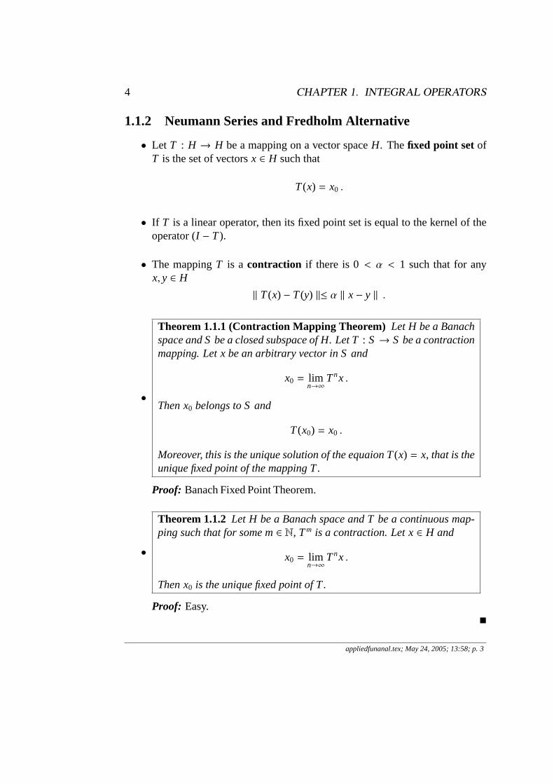
• Let T : H → H be a mapping on a vector spaceH. Thefixed point setofT is the set of vectorsx ∈ H such that
T(x) = x0 .
• If T is a linear operator, then its fixed point set is equal to the kernel of theoperator (I − T).
• The mappingT is a contraction if there is 0< α < 1 such that for anyx, y ∈ H
‖ T(x) − T(y) ‖≤ α ‖ x− y ‖ .
•
Theorem 1.1.1 (Contraction Mapping Theorem) Let H be a Banachspace and S be a closed subspace of H. Let T: S→ S be a contractionmapping. Let x be an arbitrary vector in S and
x0 = limn→∞
Tnx .
Then x0 belongs to S and
T(x0) = x0 .
Moreover, this is the unique solution of the equaion T(x) = x, that is theunique fixed point of the mapping T.
Proof: Banach Fixed Point Theorem.
•
Theorem 1.1.2 Let H be a Banach space and T be a continuous map-ping such that for some m∈ N, Tm is a contraction. Let x∈ H and
x0 = limn→∞
Tnx .
Then x0 is the unique fixed point of T .
Proof: Easy.
appliedfunanal.tex; May 24, 2005; 13:58; p. 3
1.1. EXISTENSE THEOREMS 5
•
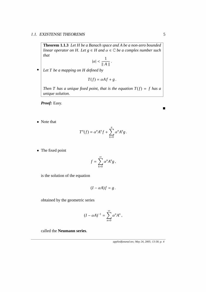
Theorem 1.1.3 Let H be a Banach space and A be a non-zero boundedlinear operator on H. Let g∈ H andα ∈ C be a complex number suchthat
|α| <1‖ A ‖
.
Let T be a mapping on H defined by
T( f ) = αA f + g .
Then T has a unique fixed point, that is the equation T( f ) = f has aunique solution.
Proof: Easy.
• Note that
Tn( f ) = αnAn f +n∑
k=0
αnAng .
• The fixed point
f =∞∑
k=0
αnAng ,
is the solution of the equation
(I − αA) f = g .
obtained by the geometric series
(I − αA)−1 =
∞∑n=0
αnAn ,
called theNeumann series.
appliedfunanal.tex; May 24, 2005; 13:58; p. 4
6 CHAPTER 1. INTEGRAL OPERATORS
•
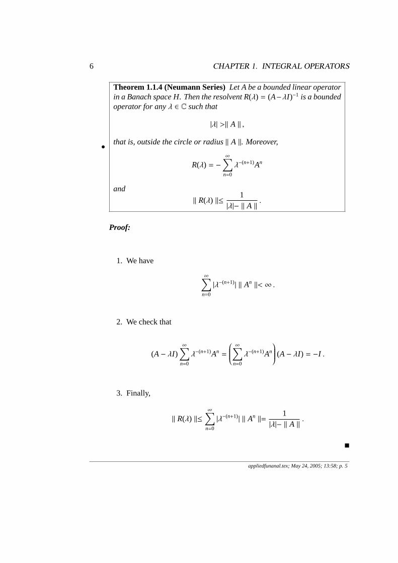
Theorem 1.1.4 (Neumann Series)Let A be a bounded linear operatorin a Banach space H. Then the resolvent R(λ) = (A−λI )−1 is a boundedoperator for anyλ ∈ C such that
|λ| >‖ A ‖ ,
that is, outside the circle or radius‖ A ‖. Moreover,
R(λ) = −∞∑
n=0
λ−(n+1)An
and
‖ R(λ) ‖≤1
|λ|− ‖ A ‖.
Proof:
1. We have
∞∑n=0
|λ−(n+1)| ‖ An ‖< ∞ .
2. We check that
(A− λI )∞∑
n=0
λ−(n+1)An =
∞∑n=0
λ−(n+1)An
(A− λI ) = −I .
3. Finally,
‖ R(λ) ‖≤∞∑
n=0
|λ−(n+1)| ‖ An ‖=1
|λ|− ‖ A ‖.
appliedfunanal.tex; May 24, 2005; 13:58; p. 5
1.1. EXISTENSE THEOREMS 7
•
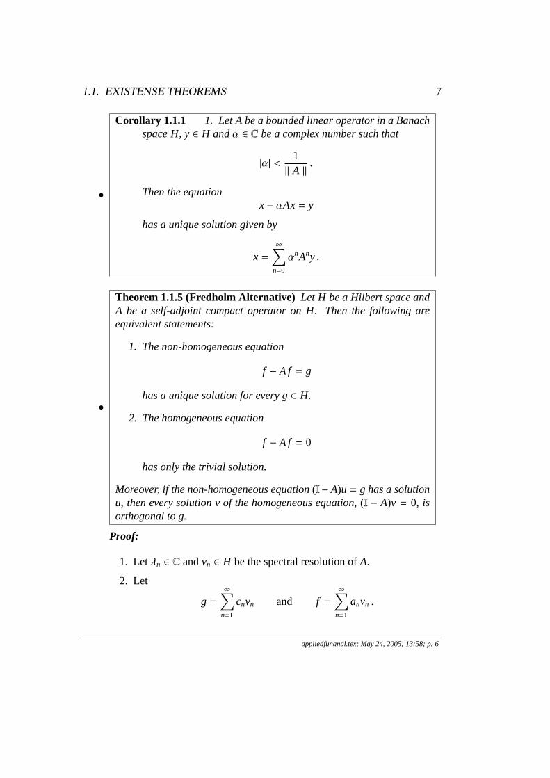
Corollary 1.1.1 1. Let A be a bounded linear operator in a Banachspace H, y∈ H andα ∈ C be a complex number such that
|α| <1‖ A ‖
.
Then the equationx− αAx= y
has a unique solution given by
x =∞∑
n=0
αnAny .
•
Theorem 1.1.5 (Fredholm Alternative) Let H be a Hilbert space andA be a self-adjoint compact operator on H. Then the following areequivalent statements:
1. The non-homogeneous equation
f − A f = g
has a unique solution for every g∈ H.
2. The homogeneous equation
f − A f = 0
has only the trivial solution.
Moreover, if the non-homogeneous equation(I− A)u = g has a solutionu, then every solution v of the homogeneous equation,(I − A)v = 0, isorthogonal to g.
Proof:
1. Letλn ∈ C andvn ∈ H be the spectral resolution ofA.
2. Let
g =∞∑
n=1
cnvn and f =∞∑
n=1
anvn .
appliedfunanal.tex; May 24, 2005; 13:58; p. 6
8 CHAPTER 1. INTEGRAL OPERATORS
3. Then for anyn ∈ N, if λn , 1, then
an =cn
1− λn.
4. So, if the non-homogeneous equation has a solution then it is uniqueand has the form
f =∞∑
n=1
cn
1− λnvn .
5. The convergence of the series follows from the fact thatλn→ 0.
6. If the homogeneous equation has a non-trivial solution, then the non-homogeneous equation has infinitely many solutions.
7. The orthogonality of the solutions follows from the equations.
1.1.3 Homework
• Exercises: 5.12[1,2,3]
appliedfunanal.tex; May 24, 2005; 13:58; p. 7
1.2. FREDHOLM INTEGRAL EQUATIONS 9
1.2 Fredholm Integral Equations
1.2.1 Hilbert-Schmidt and Trace -Class Operators
• Let H be a Hilbert space and (en) be an orthonormal basis inH. An operatorA on H is called atrace-class operatorif the series
Tr A =∞∑
n=1
(Aen,en) < ∞
converges.
• For every trace-class operatorA the operatorA∗ is trace-class and
Tr A∗ = Tr A .
• If A is a compact self-adjoint operator with the eigenvaluesλn, thenA istrace-class if and only if
∞∑n=1
|λn| < ∞ ,
where each eigenvalue is taken with its multiplicity, and
Tr A =∞∑
n=1
λn .
This is also true for non-self-adjoint operators.
• It A is a trace-class operator andB is a bounded operator, thenAB andBAare trace-class operators and
Tr (AB) = Tr (BA) .
• For a bounded operatorA the operator|A| is defined by
|A| =√
A∗A .
• An operatorA is trace-class if and only if|A| is trace-class.
• The trace-norm of a trace-class operatorA is
‖ A ‖tr= Tr |A| .
appliedfunanal.tex; May 24, 2005; 13:58; p. 8
10 CHAPTER 1. INTEGRAL OPERATORS
• For any trace-class operatorA
‖ A∗ ‖tr=‖ A ‖tr
‖ A ‖≤‖ A ‖tr
and|Tr A| ≤‖ A ‖tr
• Let A be a bounded operator on a Hilbert spaceH andA∗ be its adjoint. TheHilbert-Schmidt norm of A is defined by
‖ A ‖HS= (Tr AA∗)1/2 .
• An operatorA is called aHilbert-Schmidt operator if its Hilbert-Schmidtnorm is finite.
• There holds‖ A∗ ‖HS=‖ A ‖HS .
• The operator norm of the operatorA is related to the Hilbert-Schmidt normby
‖ A ‖≤‖ A ‖HS .
• An operatorA is Hilbert-Schmidt if and only if|A| is Hilbert-Schmidt.
• The productsAB and BA of two Hilbert-Schmidt operatorsA and B areHilbert-Schmidt operators and
Tr (AB) = Tr (BA) .
• Every trace-class opertator is Hilbert-Schmidt.
• For any trace-class operatorA
‖ A ‖≤‖ A ‖HS≤‖ A ‖tr .
• Let H = L2(M, µ) be a Hilbert space whereM is a space with a measureµ.The operatorA in H is Hilbert-Schmidt if and only if there exists a functionK ∈ L2(M × M, µ × µ) such that the operatorA is defined by
(A f)(x) =∫
Mdµ(y) K(x, y) f (y) .
appliedfunanal.tex; May 24, 2005; 13:58; p. 9
1.2. FREDHOLM INTEGRAL EQUATIONS 11
The functionK, called theSchwartz kernel of the operatorA, is defineduniquely up to a its values on a set of (µ × µ) measure zero. The Hilbert-Schmidt norm of the operatorA is
‖ A ‖HS=
(∫M
dµ(x)∫
Mdµ(y) |K(x, y)|2
)1/2
.
1.2.2 Linear Fredholm Equations
•
Definition 1.2.1 Let I = [a,b], K be a function on I× I. The operatorA on L2(I ) defined by
(A f)(x) =∫ b
ady K(x, y) f (y)
is calledFredholm integral operator with the kernel K.
•
Lemma 1.2.1 Let I = [a,b], K be a continuous function on I× I, suchthat
k =
(∫ b
adx
∫ b
ady |K(x, y)|2
)1/2
< ∞ .
Then A is Hilbert-Schmidt operator with the norm
‖ A ‖HS= k .
Proof:
1. We have (Schwartz inequality)
|(A f)(x)|2 ≤∫ b
ady|K(x, y)|2 ‖ f ‖2
2. Thus
‖ A f ‖2≤ k2 ‖ f ‖2< ∞ .
3. So,A is a bounded operator onL2(I ).
appliedfunanal.tex; May 24, 2005; 13:58; p. 10
12 CHAPTER 1. INTEGRAL OPERATORS
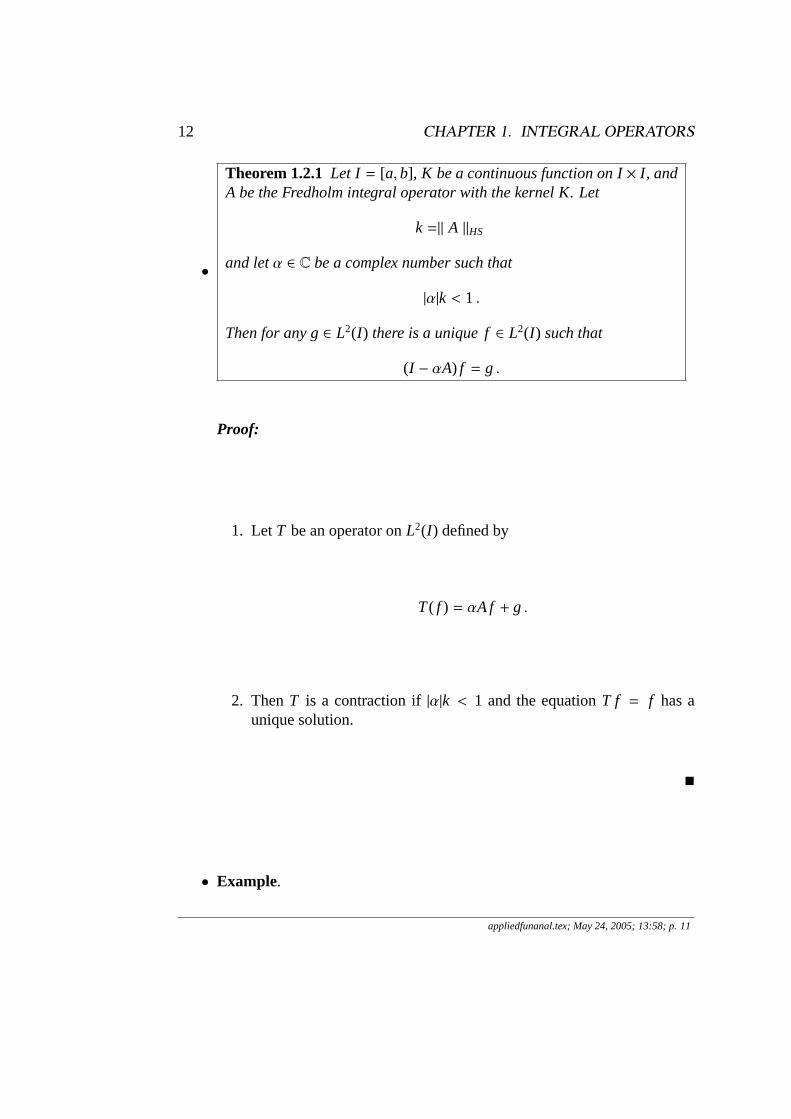
•
Theorem 1.2.1 Let I = [a,b], K be a continuous function on I× I, andA be the Fredholm integral operator with the kernel K. Let
k =‖ A ‖HS
and letα ∈ C be a complex number such that
|α|k < 1 .
Then for any g∈ L2(I ) there is a unique f∈ L2(I ) such that
(I − αA) f = g .
Proof:
1. LetT be an operator onL2(I ) defined by
T( f ) = αA f + g .
2. ThenT is a contraction if|α|k < 1 and the equationT f = f has aunique solution.
• Example.
appliedfunanal.tex; May 24, 2005; 13:58; p. 11
1.2. FREDHOLM INTEGRAL EQUATIONS 13
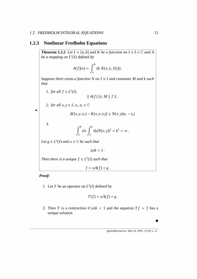
1.2.3 Nonlinear Fredholm Equations
•
Theorem 1.2.2 Let I = [a,b] and K be a function on I× I × C and Abe a mapping on L2(I ) defined by
A( f )(x) =∫ b
ady K(x, y, f (y)) .
Suppose there exists a function N on I× I and constants M and k suchthat
1. for all f ∈ L2(I )‖ A( f ) ‖≤ M ‖ f ‖ ,
2. for all x, y ∈ I, z1, z2 ∈ C
|K(x, y, z1) − K(x, y, z2)| ≤ N(x, y)|z1 − z2|
3. ∫ b
adx
∫ b
ady|N(x, y)|2 = k2 < ∞ .
Let g∈ L2(I ) andα ∈ C be such that
|α|k < 1 .
Then there is a unique f∈ L2(I ) such that
f = αA( f ) + g .
Proof:
1. LetT be an operator onL2(I ) defined by
T( f ) = αA( f ) + g .
2. ThenT is a contraction if|α|k < 1 and the equationT f = f has aunique solution.
appliedfunanal.tex; May 24, 2005; 13:58; p. 12
14 CHAPTER 1. INTEGRAL OPERATORS
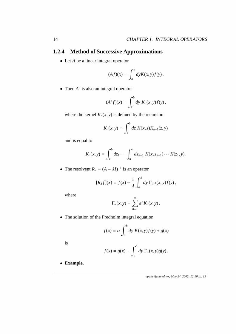
1.2.4 Method of Successive Approximations
• Let A be a linear integral operator
(A f)(x) =∫ b
adyK(x, y) f (y) .
• ThenAn is also an integral operator
(An f )(x) =∫ b
ady Kn(x, y) f (y) ,
where the kernelKn(x, y) is defined by the recursion
Kn(x, y) =∫ b
adz K(x, z)Kn−1(z, y)
and is equal to
Kn(x, y) =∫ b
adz1 · · ·
∫ b
adzn−1 K(x, zn−1) · · ·K(z1, y) .
• The resolventRλ = (A− λI )−1 is an operator
[Rλ f ](x) = f (x) −1λ
∫ b
adyΓλ−1(x, y) f (y) ,
where
Γα(x, y) =∞∑
n=1
αnKn(x, y) .
• The solution of the Fredholm integral equation
f (x) = α∫ b
ady K(x, y) f (y) + g(x)
is
f (x) = g(x) +∫ b
adyΓα(x, y)g(y) .
• Example.
appliedfunanal.tex; May 24, 2005; 13:58; p. 13
1.2. FREDHOLM INTEGRAL EQUATIONS 15
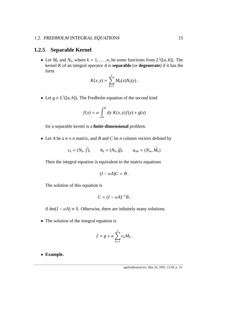
1.2.5 Separable Kernel
• Let Mk andNk, wherek = 1, . . . ,n, be some functions fromL2([a,b]). ThekernelK of an integral operatorA is separable(or degenerate) if it has theform
K(x, y) =n∑
k=1
Mk(x)Nk(y) .
• Let g ∈ L2([a,b]). The Fredholm equation of the second kind
f (x) = α∫ b
ady K(x, y) f (y) + g(x)
for a separable kernel is afinite-dimensionalproblem.
• Let A be an× n matrix, andB andC ben column vectors defined by
ck = (Nk, f ), bk = (Nk, g), amk = (Nm, Mk)
Then the integral equation is equivalent to the matrix equations
(I − αA)C = B .
The solution of this equation is
C = (I − αA)−1B ,
if det(I − αA) , 0. Otherwise, there are infinitely many solutions.
• The solution of the integral equation is
f = g+ αn∑
k=1
ckMk .
• Example.
appliedfunanal.tex; May 24, 2005; 13:58; p. 14
16 CHAPTER 1. INTEGRAL OPERATORS
1.2.6 Convolution Kernel
• Let K be integrable functions onR from L1(R). An integral operatorA onL1(R) with the kernel of the form
K(x, y) = K(x− y)
is called theconvolution operator and the kernelK(x − y) is called theconvolution kernel.
• Let g ∈ L1(R). Fredholm equation with convolution kernel is the equation
f (x) = α∫ ∞
−∞
dy K(x− y) f (y) + g(x) .
orf = α
√2πK ∗ f + g .
where∗ is the convolution.
• Applying the Fourier transform we get
f = α(2π)1/2K f + g .
The formal solution is given by the inverse Fourier transform
f = F
(g
1− α√
2πK
)or
f (x) =∫ ∞
−∞
dω eiωx
(g(ω)
1− α√
2πK(ω)
)
1.2.7 Hilbert Transform
• We consider smooth functions with compact support onR from C∞0 (R).
• The Cauchy principal value integral is defined by
P∫ ∞
−∞
dy f(y) = limε→0+
(∫ −ε
−∞
+
∫ ∞
ε
)dy f(y) .
appliedfunanal.tex; May 24, 2005; 13:58; p. 15
1.2. FREDHOLM INTEGRAL EQUATIONS 17
• TheHilbert transform is the operatorH on this space by
(H f )(x) = P∫ ∞
−∞
dyf (y)x− y
.
• Proposition. The Hilbert transform is an anti-involution
H2 = −Id .
That is the inverse Hilbert tranform is given by
H−1 = −H .
Proof: Use Fourier transform.
1.2.8 Homework
• Exercises: 5.12[4,6,7,8,11,12,13,14,15,32]. In each exercise that has manysubproblems, a,b,c, . . . , do only one problem of your choice.
appliedfunanal.tex; May 24, 2005; 13:58; p. 16
18 CHAPTER 1. INTEGRAL OPERATORS
1.3 Volterra Integral Equations
•
Definition 1.3.1 Let I = [a,b], K be a function on I× I. The operatorA on L2(I ) defined by
(A f)(x) =∫ x
ady K(x, y) f (y)
is calledVolterra integral operator with the kernel K.
1.3.1 Volterra Equations of the Second Kind
•
Theorem 1.3.1 Let I = [a,b], K be a function on I× I with the Hilbert-Schmidt norm k, and A be the Volterra integral operator with the kernelK. Then for any g∈ L2(I ) and for anyα ∈ C there exists a uniquef ∈ L2(I ) such that
f = αA f + g .
The solution f of this equation has the form
f = g+∞∑
n=1
αnAng ,
where An is the Volterra integral operator with the kernel
Kn(x, y) =∫ x
adzn−1 · · ·
∫ z2
adz1K(x, zn−1) · · ·K(z1, y) ,
Proof:
1. LetT be a mapping onL2(I ) defined by
T( f ) = αA f + g .
2. Then
Tn( f ) = αnAn f +n−1∑k=0
αkAkg .
3. Then for anyn ≥ 2 we have
‖ Tn( f1) − Tn( f2) ‖2≤|α|2nkn
(n− 1)!‖ f1 − f2 ‖
2 .
appliedfunanal.tex; May 24, 2005; 13:58; p. 17
1.3. VOLTERRA INTEGRAL EQUATIONS 19
4. There exists anm ∈ N such thatTm is a contraction.
5. ThusT( f ) = f has a unique solution given by
f = limn→∞
Tn( f ) .
•
Corollary 1.3.1 (Homogeneous Volterra Equation.)Let I = [a,b], Kbe a function on I× I with the finite Hilbert-Schmidt norm k and A bethe Volterra intergal operator on L2(I ) with the kernel K. Then for anyα ∈ C the equation
f = αA f
has only the trivial solution f= 0. Thus, the operator A does not haveany eigenvalues, the resolvent Rα is a bounded operator for anyα ∈ C,and the spectrumσ(A) is empty.
Proof: Follows from the previous theorem.
1.3.2 Volterra Equations of the First Kind
• Let I = [a,b] andg ∈ L2(I ), K be a function onI × I , andA be the Volterraintegral operator onL2(I ) with the kernelK and a finite Hilbert-Schmidtnorm. TheVolterra equation of the first kind has the form
A f = g .
• Suppose thatg andK are differentiable andK(x, x) , 0. Then
K(x, x) f (x) +∫ x
ady ∂xK(x, y) f (y) = g′(x) ,
and, therefore, we get a Volterra equation of the second kind
f (x) +∫ x
ady N(x, y) f (y) = h(x) ,
where
N(x, y) =∂xK(x, y)K(x, x)
appliedfunanal.tex; May 24, 2005; 13:58; p. 18
20 CHAPTER 1. INTEGRAL OPERATORS
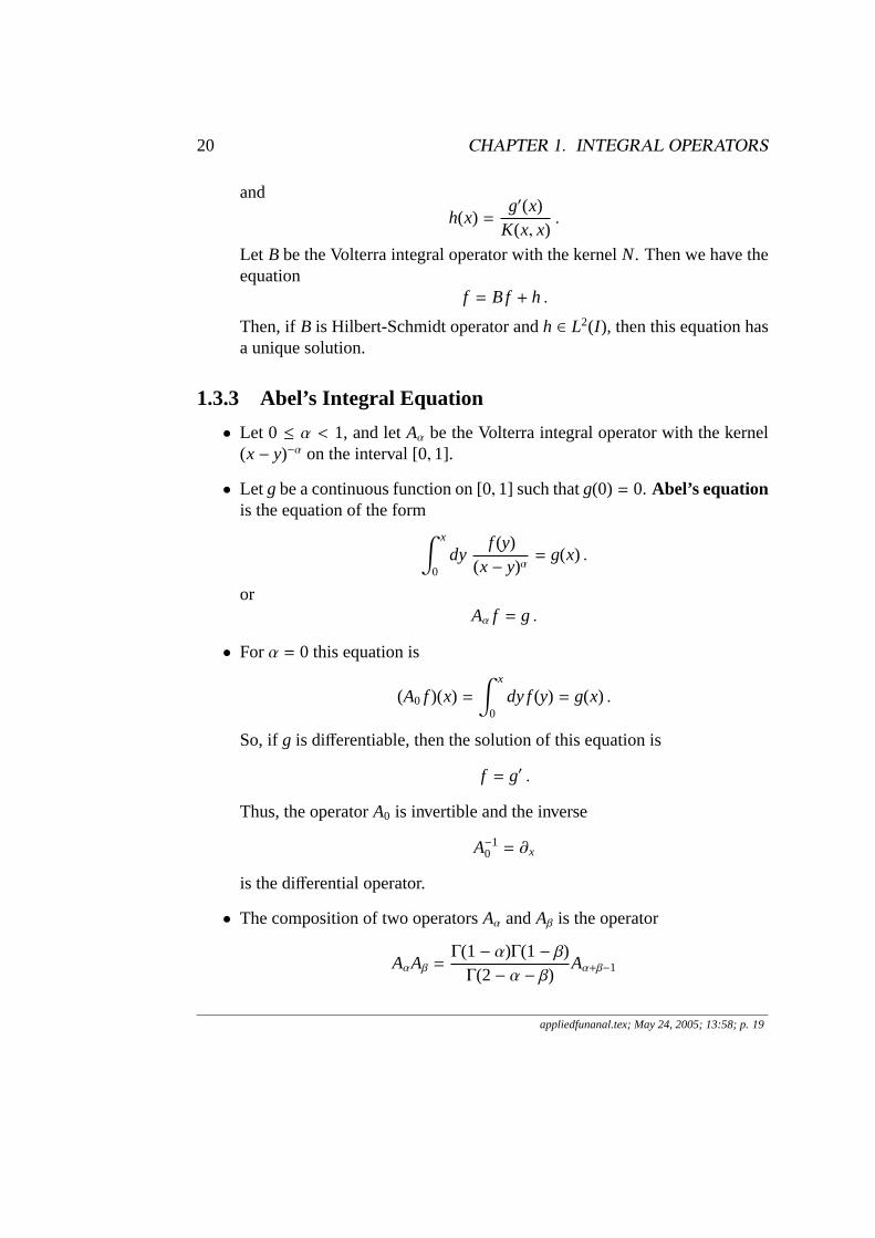
and
h(x) =g′(x)
K(x, x).
Let B be the Volterra integral operator with the kernelN. Then we have theequation
f = B f + h .
Then, if B is Hilbert-Schmidt operator andh ∈ L2(I ), then this equation hasa unique solution.
1.3.3 Abel’s Integral Equation
• Let 0 ≤ α < 1, and letAα be the Volterra integral operator with the kernel(x− y)−α on the interval [0,1].
• Let g be a continuous function on [0,1] such thatg(0) = 0. Abel’s equationis the equation of the form∫ x
0dy
f (y)(x− y)α
= g(x) .
orAα f = g .
• Forα = 0 this equation is
(A0 f )(x) =∫ x
0dy f(y) = g(x) .
So, if g is differentiable, then the solution of this equation is
f = g′ .
Thus, the operatorA0 is invertible and the inverse
A−10 = ∂x
is the differential operator.
• The composition of two operatorsAα andAβ is the operator
AαAβ =Γ(1− α)Γ(1− β)Γ(2− α − β)
Aα+β−1
appliedfunanal.tex; May 24, 2005; 13:58; p. 19
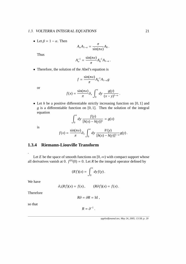
1.3. VOLTERRA INTEGRAL EQUATIONS 21
• Let β = 1− α. Then
AαA1−α =π
sin(πα)A0 .
Thus
A−1α =
sin(πα)π
A−10 A1−α .
• Therefore, the solution of the Abel’s equation is
f =sin(πα)π
A−10 A1−αg
or
f (x) =sin(πα)π
∂x
∫ x
0dy
g(y)(x− y)1−α
.
• Let h be a positive differentiable strictly increasing function on [0,1] andg is a differentiable function on [0,1]. Then the solution of the integralequation ∫ x
0dy
f (y)[h(x) − h(y)]α
= g(x)
is
f (x) =sin(πα)π
∂x
∫ x
0dy
h′(y)[h(x) − h(y)]1−α
g(y) .
1.3.4 Riemann-Liouville Transform
.Let E be the space of smooth functions on [0,∞) with compact support whose
all derivatives vanish at 0.f (k)(0) = 0. LetRbe the integral operator defined by
(R f)(x) =∫ x
0dy f(y) .
We have∂x(R f)(x) = f (x) , (R∂ f )(x) = f (x) .
ThereforeR∂ = ∂R= Id ,
so thatR= ∂−1 .
appliedfunanal.tex; May 24, 2005; 13:58; p. 20
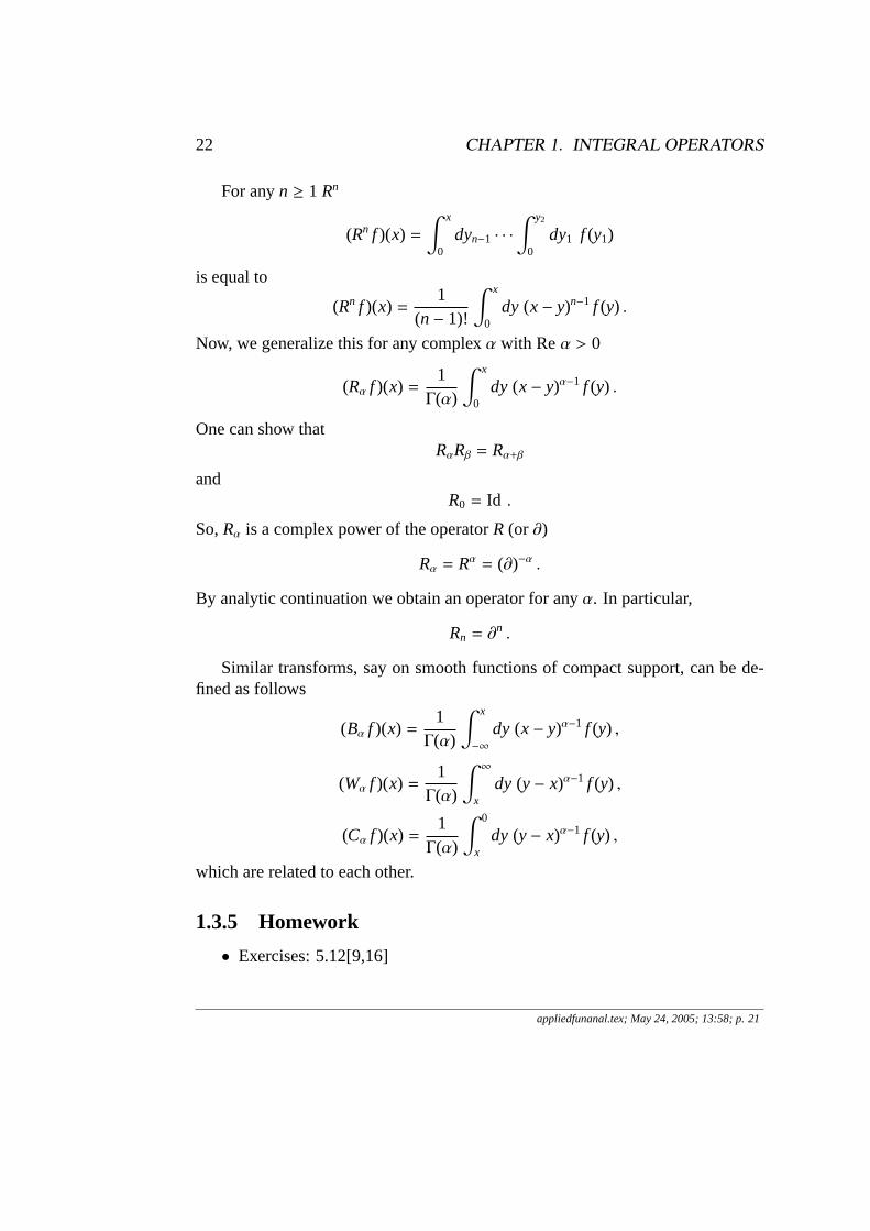
22 CHAPTER 1. INTEGRAL OPERATORS
For anyn ≥ 1 Rn
(Rn f )(x) =∫ x
0dyn−1 · · ·
∫ y2
0dy1 f (y1)
is equal to
(Rn f )(x) =1
(n− 1)!
∫ x
0dy (x− y)n−1 f (y) .
Now, we generalize this for any complexα with Reα > 0
(Rα f )(x) =1Γ(α)
∫ x
0dy (x− y)α−1 f (y) .
One can show thatRαRβ = Rα+β
andR0 = Id .
So,Rα is a complex power of the operatorR (or ∂)
Rα = Rα = (∂)−α .
By analytic continuation we obtain an operator for anyα. In particular,
Rn = ∂n .
Similar transforms, say on smooth functions of compact support, can be de-fined as follows
(Bα f )(x) =1Γ(α)
∫ x
−∞
dy (x− y)α−1 f (y) ,
(Wα f )(x) =1Γ(α)
∫ ∞
xdy (y− x)α−1 f (y) ,
(Cα f )(x) =1Γ(α)
∫ 0
xdy (y− x)α−1 f (y) ,
which are related to each other.
1.3.5 Homework
• Exercises: 5.12[9,16]
appliedfunanal.tex; May 24, 2005; 13:58; p. 21
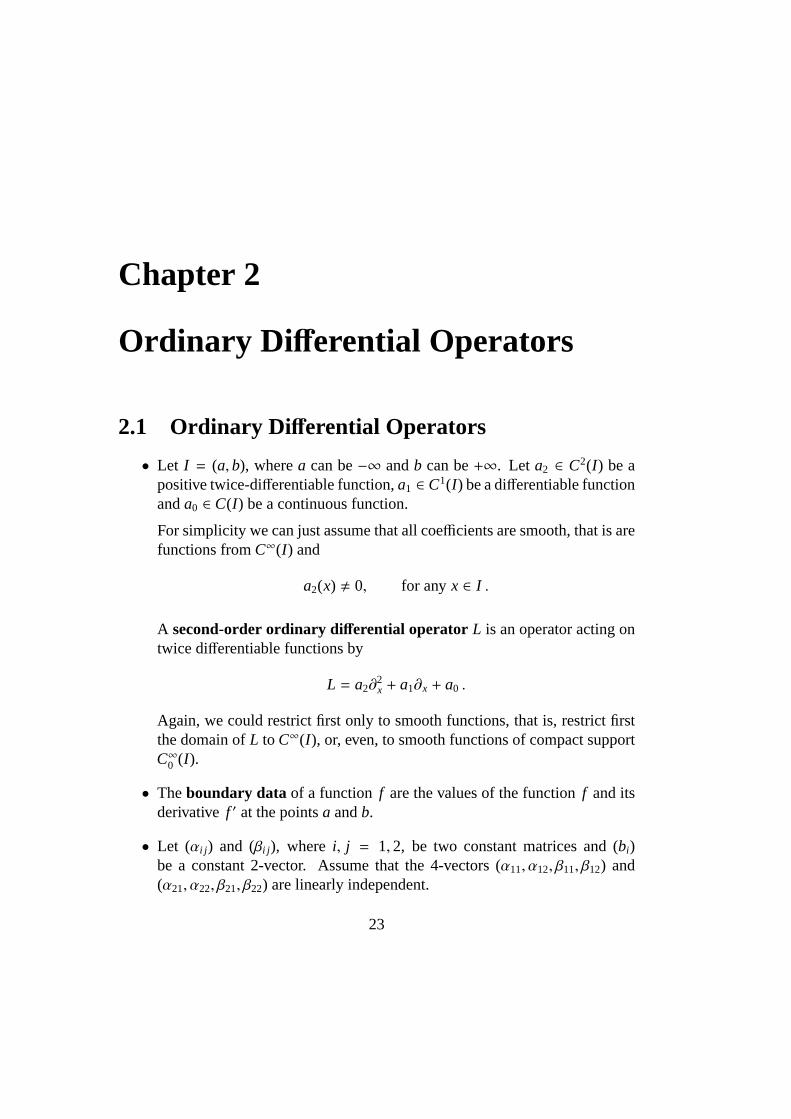
Chapter 2
Ordinary Di fferential Operators
2.1 Ordinary Differential Operators
• Let I = (a,b), wherea can be−∞ andb can be+∞. Let a2 ∈ C2(I ) be apositive twice-differentiable function,a1 ∈ C1(I ) be a differentiable functionanda0 ∈ C(I ) be a continuous function.
For simplicity we can just assume that all coefficients are smooth, that is arefunctions fromC∞(I ) and
a2(x) , 0, for anyx ∈ I .
A second-order ordinary differential operator L is an operator acting ontwice differentiable functions by
L = a2∂2x + a1∂x + a0 .
Again, we could restrict first only to smooth functions, that is, restrict firstthe domain ofL to C∞(I ), or, even, to smooth functions of compact supportC∞0 (I ).
• Theboundary data of a function f are the values of the functionf and itsderivative f ′ at the pointsa andb.
• Let (αi j ) and (βi j ), where i, j = 1,2, be two constant matrices and (bi)be a constant 2-vector. Assume that the 4-vectors (α11, α12, β11, β12) and(α21, α22, β21, β22) are linearly independent.
23
24 CHAPTER 2. ORDINARY DIFFERENTIAL OPERATORS
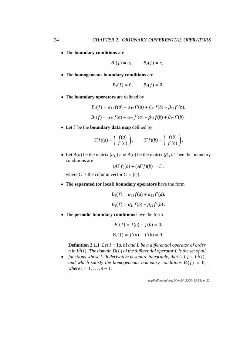
• Theboundary conditionsare
B1( f ) = c1, B2( f ) = c2 .
• Thehomogeneous boundary conditionsare
B1( f ) = 0, B2( f ) = 0 .
• Theboundary operatorsare defined by
B1( f ) = α11 f (a) + α12 f ′(a) + β11 f (b) + β12 f ′(b),
B2( f ) = α21 f (a) + α22 f ′(a) + β21 f (b) + β22 f ′(b) .
• Let Γ be theboundary data mapdefined by
(Γ f )(a) =
(f (a)f ′(a)
), (Γ f )(b) =
(f (b)f ′(b)
),
• Let A(a) be the matrix (αi j ) andA(b) be the matrix (βi j ). Then the boundaryconditions are
(AΓ f )(a) + (AΓ f )(b) = C ,
whereC is the column vectorC = (ci).
• Theseparated (or local) boundary operatorshave the form
B1( f ) = α11 f (a) + α12 f ′(a),
B2( f ) = β21 f (b) + β22 f ′(b) .
• Theperiodic boundary conditionshave the form
B1( f ) = f (a) − f (b) = 0,
B2( f ) = f ′(a) − f ′(b) = 0 .
•
Definition 2.1.1 Let I = [a,b] and L be a differential operator of ordern in L2(I ). The domain D(L) of the differential operator L is the set of allfunctions whose k-th derivative is square integrable, that is L f∈ L2(I ),and which satisfy the homogeneous boundary conditions Bi( f ) = 0,where i= 1, . . . ,n− 1.
appliedfunanal.tex; May 24, 2005; 13:58; p. 22
2.1. ORDINARY DIFFERENTIAL OPERATORS 25
•
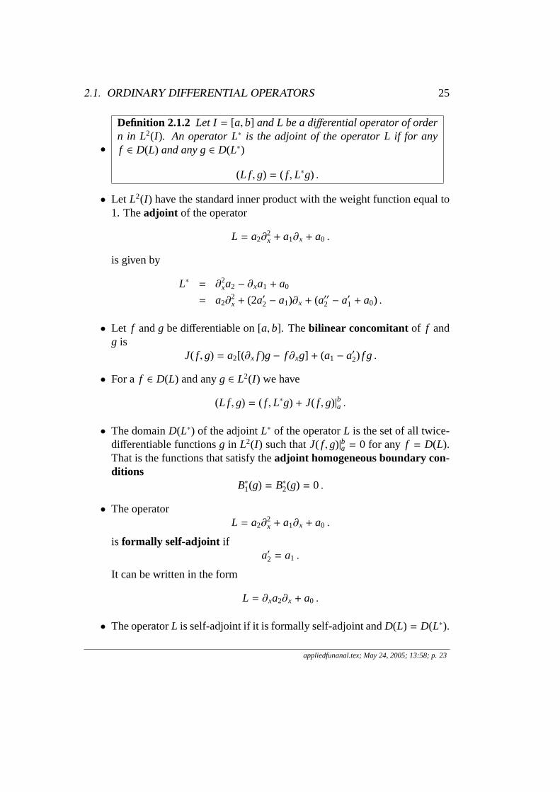
Definition 2.1.2 Let I = [a,b] and L be a differential operator of ordern in L2(I ). An operator L∗ is the adjoint of the operator L if for anyf ∈ D(L) and any g∈ D(L∗)
(L f ,g) = ( f , L∗g) .
• Let L2(I ) have the standard inner product with the weight function equal to1. Theadjoint of the operator
L = a2∂2x + a1∂x + a0 .
is given by
L∗ = ∂2xa2 − ∂xa1 + a0
= a2∂2x + (2a′2 − a1)∂x + (a′′2 − a′1 + a0) .
• Let f andg be differentiable on [a,b]. Thebilinear concomitant of f andg is
J( f ,g) = a2[(∂x f )g− f∂xg] + (a1 − a′2) f g .
• For a f ∈ D(L) and anyg ∈ L2(I ) we have
(L f ,g) = ( f , L∗g) + J( f ,g)|ba .
• The domainD(L∗) of the adjointL∗ of the operatorL is the set of all twice-differentiable functionsg in L2(I ) such thatJ( f ,g)|ba = 0 for any f = D(L).That is the functions that satisfy theadjoint homogeneous boundary con-ditions
B∗1(g) = B∗2(g) = 0 .
• The operatorL = a2∂
2x + a1∂x + a0 .
is formally self-adjoint ifa′2 = a1 .
It can be written in the form
L = ∂xa2∂x + a0 .
• The operatorL is self-adjoint if it is formally self-adjoint andD(L) = D(L∗).
appliedfunanal.tex; May 24, 2005; 13:58; p. 23
26 CHAPTER 2. ORDINARY DIFFERENTIAL OPERATORS
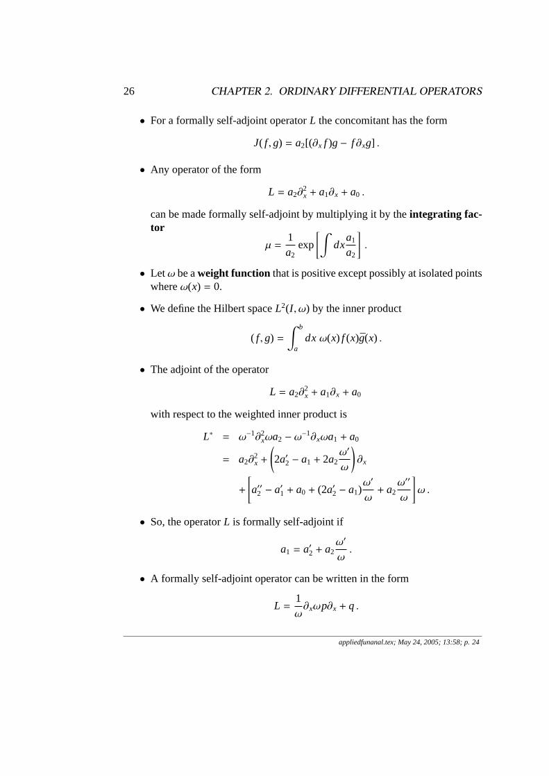
• For a formally self-adjoint operatorL the concomitant has the form
J( f ,g) = a2[(∂x f )g− f∂xg] .
• Any operator of the form
L = a2∂2x + a1∂x + a0 .
can be made formally self-adjoint by multiplying it by theintegrating fac-tor
µ =1a2
exp
[∫dx
a1
a2
].
• Letω be aweight function that is positive except possibly at isolated pointswhereω(x) = 0.
• We define the Hilbert spaceL2(I , ω) by the inner product
( f ,g) =∫ b
adxω(x) f (x)g(x) .
• The adjoint of the operator
L = a2∂2x + a1∂x + a0
with respect to the weighted inner product is
L∗ = ω−1∂2xωa2 − ω
−1∂xωa1 + a0
= a2∂2x +
(2a′2 − a1 + 2a2
ω′
ω
)∂x
+
[a′′2 − a′1 + a0 + (2a′2 − a1)
ω′
ω+ a2
ω′′
ω
]ω .
• So, the operatorL is formally self-adjoint if
a1 = a′2 + a2ω′
ω.
• A formally self-adjoint operator can be written in the form
L =1ω∂xωp∂x + q .
appliedfunanal.tex; May 24, 2005; 13:58; p. 24
2.1. ORDINARY DIFFERENTIAL OPERATORS 27
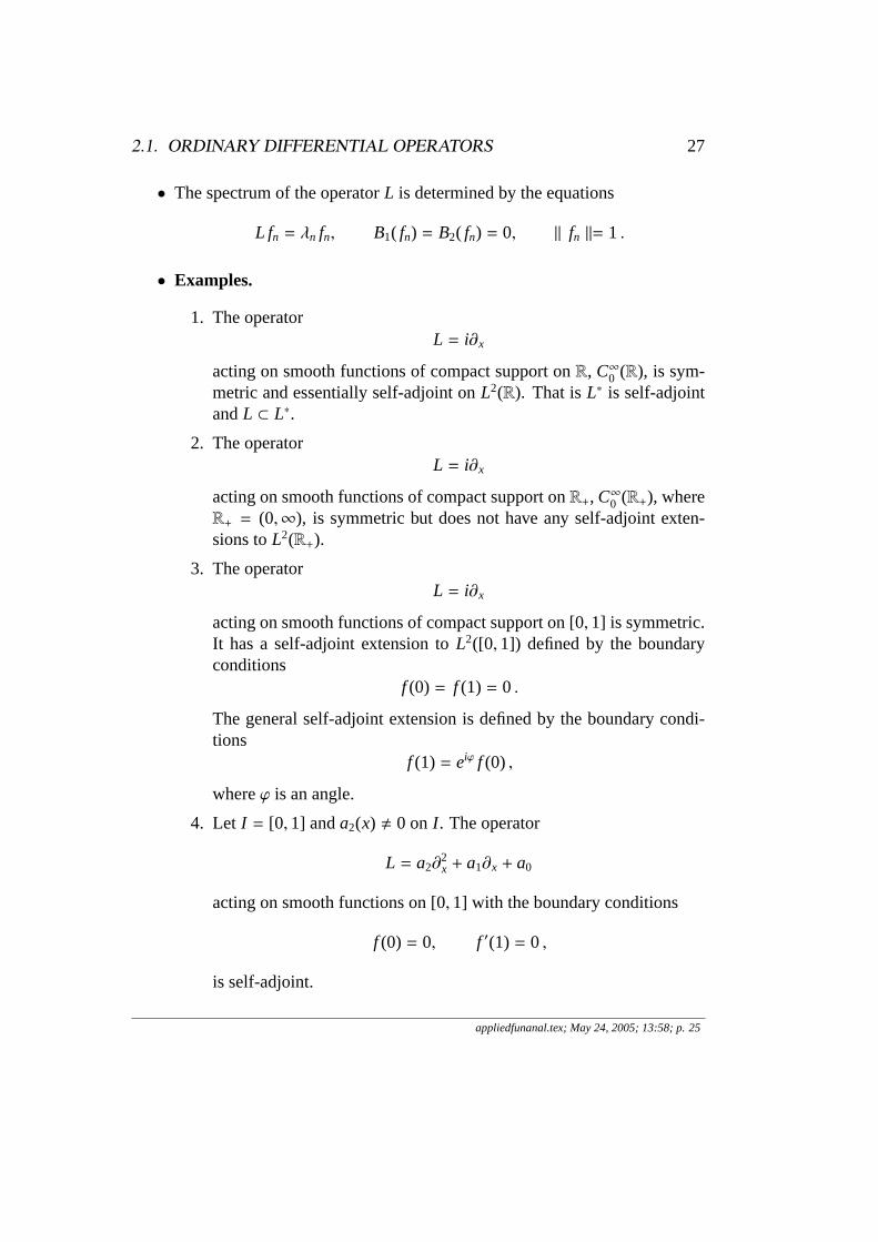
• The spectrum of the operatorL is determined by the equations
L fn = λn fn, B1( fn) = B2( fn) = 0, ‖ fn ‖= 1 .
• Examples.
1. The operatorL = i∂x
acting on smooth functions of compact support onR, C∞0 (R), is sym-metric and essentially self-adjoint onL2(R). That isL∗ is self-adjointandL ⊂ L∗.
2. The operatorL = i∂x
acting on smooth functions of compact support onR+, C∞0 (R+), whereR+ = (0,∞), is symmetric but does not have any self-adjoint exten-sions toL2(R+).
3. The operatorL = i∂x
acting on smooth functions of compact support on [0,1] is symmetric.It has a self-adjoint extension toL2([0,1]) defined by the boundaryconditions
f (0) = f (1) = 0 .
The general self-adjoint extension is defined by the boundary condi-tions
f (1) = eiϕ f (0) ,
whereϕ is an angle.
4. Let I = [0,1] anda2(x) , 0 on I . The operator
L = a2∂2x + a1∂x + a0
acting on smooth functions on [0,1] with the boundary conditions
f (0) = 0, f ′(1) = 0 ,
is self-adjoint.
appliedfunanal.tex; May 24, 2005; 13:58; p. 25
28 CHAPTER 2. ORDINARY DIFFERENTIAL OPERATORS
5. The operatorL = −∂2
x
acting on smooth functions on [0,1] with the boundary conditions
f (0) = 0 , f ′(0) = 0 ,
is not self-adjoint.
6. The operatorL = −∂2
x
acting on smooth functions onR+ with compact support is symmetric.It has a symmetric extension defined by the boundary conditions
f (0) = 0 ,
which is essentially self-adjoint onL2(R+).The most general self-adjoint extension of the operatorL is defined bythe boundary conditions
cosϕ f (0)+ sinϕ f ′(0) = 0 ,
whereϕ is an arbitrary angle.
7. Legendre, Associated Legendre, Chebyshev, Jacobi, Laguerre, Asso-ciated Laguerre, Bessel, Hermite, operators.
2.1.1 Homework
• Exercises: 5.12[17,19,21,]
• Find the spectrum (eigenvalues and the eigenfunctions) of the operatorsL =−∂2
x on the interval [a,b] with the following boundary conditions
1. Dirichletf (a) = f (b) = 0 ,
2. Neumannf ′(a) = f ′(b) = 0 ,
3. Zarembaf (a) = f ′(b) = 0 ,
4. Periodicf (a) = f (b) .
appliedfunanal.tex; May 24, 2005; 13:58; p. 26
2.2. STURM-LIOUVILLE SYSTEMS 29
2.2 Sturm-Liouville Systems
• Let I = [a,b] be an interval,ω be a smooth real-valued positive function onI , i.e. ω(x) > 0 for anyx ∈ I , be a smooth real-valued positive function onI , i.e. p(x) > 0 for anyx ∈ I , andq be a smooth real-valued function onI .
• Let L be a differential operator acting on smooth functions,f ∈ C∞(I ), on Idefined by
L = −ω−1∂xωp∂x + q .
• Let B be the boundary operator defined by
B f = (u f + v f ′)|∂I ,
whereu andv are some real-valued functions of the boundary ofI , consist-ing of two points,∂I = a,b, which are not simultaneously zero, that isu2 + v2 > 0 .
• Let L2(I , ω) be the Hilbert space with the weight functionω and‖ · ‖ be thecorresponding norm. Aregular Sturm-Lioville system is the boundaryvalue problem
L f = λ f , ‖ f ‖= 1 ,
with the homogeneous boundary conditions
B f = 0 .
• If the function p is positive only on an open interval (a,b) but vanishes atone or both endpoints of the interval [a,b], then the boundary conditionB fat that point is replaced by the condition thatf must be bounded at thatpoint. Such a boundary value problem is called asingular Sturm-Liovillesystem.
• If the functionsp, ω, andq are periodic, that isp(a) = p(b), ω(a) = ω(b)andq(a) = q(b), and the boundary conditions are periodic, that is,
f (a) = f (b), f ′(a) = f ′(b) ,
then the boundary value problem is called aperiodic Sturm-Lioville sys-tem.
appliedfunanal.tex; May 24, 2005; 13:58; p. 27
30 CHAPTER 2. ORDINARY DIFFERENTIAL OPERATORS
• Examples.
• The domain ofL
D(L) = f ∈ L2(I , ω)| f ′′ ∈ L2(I , ω), B f |∂I = 0
is the space of all complex valued functionsf on I for which f ′′ is in L2(I , ω)and which satisfy the boundary conditions.
•
Theorem 2.2.1 (Lagrange Indentity) . For any f,g ∈ D(L) thereholds
f Lg− (L f )g = −ω−1∂x[ωp( f∂xg− (∂x f )g)] .
Proof: Computation.
•
Theorem 2.2.2 (Abel’s Formula) . Let f and g be two eigenfunctionsof the operator L corresponding to the same eigenvalueλ,
L f = λ f , Lg = λg .
ThenpW( f ,g) = const,
where( f ,g) is the Wronskian defined by
W( f ,g) = f∂xg− (∂x f )g .
Proof: Integrate Lagrange identity froma to x and use the boundary condi-tions.
•Theorem 2.2.3 The eigenvalues of a regular Sturm-Lioville system aresimple, that is, have multiplicity one.
Proof: Use Abel formula and the boundary conditions.
• Theorem 2.2.4 L is a self-adjoint operator on L2(I , ω).
Proof: Integrate Lagrange identity froma to b and use the boundary condi-tions.
appliedfunanal.tex; May 24, 2005; 13:58; p. 28
2.2. STURM-LIOUVILLE SYSTEMS 31
• Theorem 2.2.5 The eigenvalues of a Sturm-Lioville system are real.
Proof: Easy.
• Remark. The eigenvalues of a regular Sturm-Liouville system form aninfinite sequence,λn, such thatλn→ ∞. (Will prove later).
•Theorem 2.2.6 The eigenfunctions corresponding to distinct eigenval-ues of a Sturm-Lioville system are orthogonal in L2(I , ω).
Proof: Easy.
2.2.1 Homework
• Exercises: 5.12[18,19,21,22,23,24,25]
appliedfunanal.tex; May 24, 2005; 13:58; p. 29
32 CHAPTER 2. ORDINARY DIFFERENTIAL OPERATORS
2.3 Green Functions
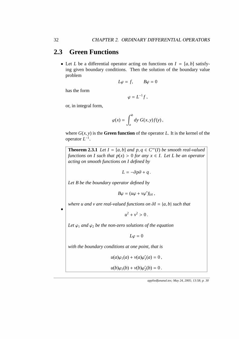
• Let L be a differential operator acting on functions onI = [a,b] satisfy-ing given boundary conditions. Then the solution of the boundary valueproblem
Lϕ = f , Bϕ = 0
has the formϕ = L−1 f ,
or, in integral form,
ϕ(x) =∫ b
ady G(x, y) f (y) ,
whereG(x, y) is theGreen function of the operatorL. It is the kernel of theoperatorL−1.
•
Theorem 2.3.1 Let I = [a,b] and p,q ∈ C∞(I ) be smooth real-valuedfunctions on I such that p(x) > 0 for any x∈ I. Let L be an operatoracting on smooth functions on I defined by
L = −∂p∂ + q .
Let B be the boundary operator defined by
Bϕ = (uϕ + vϕ′)|∂I ,
where u and v are real-valued functions on∂I = a,b such that
u2 + v2 > 0 .
Letϕ1 andϕ2 be the non-zero solutions of the equation
Lϕ = 0
with the boundary conditions at one point, that is
u(a)ϕ1(a) + v(a)ϕ′1(a) = 0 ,
u(b)ϕ2(b) + v(b)ϕ′2(b) = 0 .
appliedfunanal.tex; May 24, 2005; 13:58; p. 30
2.3. GREEN FUNCTIONS 33
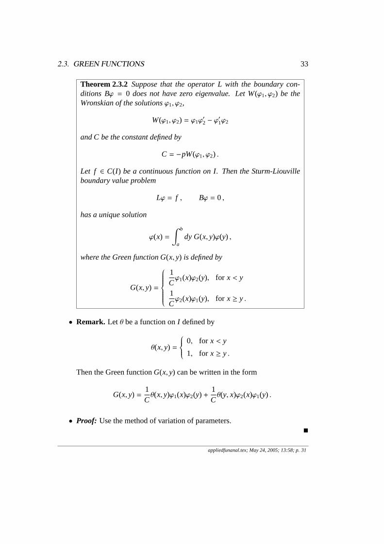
Theorem 2.3.2 Suppose that the operator L with the boundary con-ditions Bϕ = 0 does not have zero eigenvalue. Let W(ϕ1, ϕ2) be theWronskian of the solutionsϕ1, ϕ2,
W(ϕ1, ϕ2) = ϕ1ϕ′2 − ϕ
′1ϕ2
and C be the constant defined by
C = −pW(ϕ1, ϕ2) .
Let f ∈ C(I ) be a continuous function on I. Then the Sturm-Liouvilleboundary value problem
Lϕ = f , Bϕ = 0 ,
has a unique solution
ϕ(x) =∫ b
ady G(x, y)ϕ(y) ,
where the Green function G(x, y) is defined by
G(x, y) =
1Cϕ1(x)ϕ2(y), for x < y
1Cϕ2(x)ϕ1(y), for x ≥ y .
• Remark. Let θ be a function onI defined by
θ(x, y) =
0, for x < y
1, for x ≥ y .
Then the Green functionG(x, y) can be written in the form
G(x, y) =1Cθ(x, y)ϕ1(x)ϕ2(y) +
1Cθ(y, x)ϕ2(x)ϕ1(y) .
• Proof: Use the method of variation of parameters.
appliedfunanal.tex; May 24, 2005; 13:58; p. 31
34 CHAPTER 2. ORDINARY DIFFERENTIAL OPERATORS
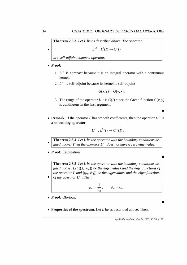
•
Theorem 2.3.3 Let L be as described above. The operator
L−1 : L2(I )→ C(I )
is a self-adjoint compact operator.
• Proof:
1. L−1 is compact because it is an integral operator with a continuouskernel.
2. L−1 is self-adjoint because its kernel is self-adjoint
G(x, y) = G(y, x) .
3. The range of the operatorL−1 is C(I ) since the Green functionG(x, y)is continuous in the first argument.
• Remark. If the operatorL has smooth coefficients, then the operatorL−1 isasmoothing operator
L−1 : L2(I )→ C∞(I ) .
•Theorem 2.3.4 Let L be the operator with the boundary conditions de-fined above. Then the operator L−1 does not have a zero eigenvalue.
• Proof: Calculation.
•
Theorem 2.3.5 Let L be the operator with the boundary conditions de-fined above. Let(λn, ϕn) be the eigenvalues and the eigenfunctions ofthe operator L and(µn, ψn) be the eigenvalues and the eigenfunctionsof the operator L−1. Then
µn =1λn, ψn = ϕn .
• Proof: Obvious.
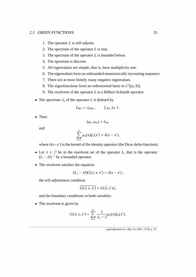
• Properties of the spectrum. Let L be as described above. Then:
appliedfunanal.tex; May 24, 2005; 13:58; p. 32
2.3. GREEN FUNCTIONS 35
1. The operatorL is self-adjoint.
2. The spectrum of the operatorL is real.
3. The spectrum of the operatorL is bounded below.
4. The spectrum is discrete.
5. All eigenvalues are simple, that is, have multiplicity one.
6. The eigenvalues form an unbounded monotonically increasing sequence.
7. There are at most finitely many negative eigenvalues.
8. The eigenfunctions form an orthonormal basis inL2([a,b]).
9. The resolvent of the operatorL is a Hilbert-Schmidt operator.
• The spectrumλn of the operatorL is defined by
Lϕn = λnϕn , ‖ ϕn ‖= 1 .
• Then(ϕn, ϕm) = δnm
and∞∑
n=1
ϕn(x)ϕn(x′) = δ(x− x′) ,
whereδ(x−x′) is the kernel of the identity operator (the Dirac delta-function).
• Let λ ∈ C be in the resolvent set of the operatorL, that is the operator(L − λI )−1 be a bounded operator.
• The resolvent satisfies the equation
(Lx − λI )G(λ; x, x′) = δ(x− x′) ,
the self-adjointness condition
G(λ; x, x′) = G(λ; x′x) ,
and the boundary conditions in both variables.
• The resolvent is given by
G(λ; x, x′) =∞∑
n=1
1λn − λ
ϕn(x)ϕn(x′) .
appliedfunanal.tex; May 24, 2005; 13:58; p. 33

36 CHAPTER 2. ORDINARY DIFFERENTIAL OPERATORS
• Let C be a contour in the complex plane going around the spectrum in thecounterclockwise direction from∞ + iε to ∞ − iε. Then a functionf (L)of the operatorL can be defined in terms of the resolvent by the Cauchyformula
f (L) = −1
2πi
∫C
dλ f (λ)G(λ) .
The kernel of this operator is
f (L)(x, x′) = −1
2πi
∫C
dλ f (λ)G(λ; x, x′)
=
∞∑n=1
f (λn)ϕn(x)ϕn(x′) .
• In some cases, depending on the functionf one can define theL2-trace by
TrL2 f (L) =∫ b
adx f(L)(x, x)
=
∞∑n=1
f (λn) .
• In particular, fort > 0 we define the heat kernel
U(t; x, x′) = −1
2πi
∫C
dλ e−tλG(λ; x, x′)
=
∞∑n=1
e−tλnϕn(x)ϕn(x′)
and its trace
Θ(t) = Tr L2 exp(−tL)
=
∫ b
adx U(t; x, x)
=
∞∑n=1
e−tλn .
appliedfunanal.tex; May 24, 2005; 13:58; p. 34
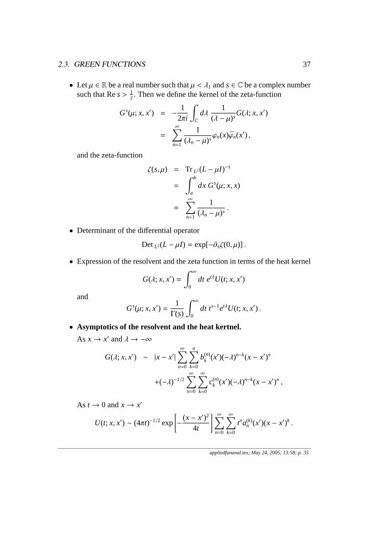
2.3. GREEN FUNCTIONS 37
• Letµ ∈ R be a real number such thatµ < λ1 ands ∈ C be a complex numbersuch that Res> 1
2. Then we define the kernel of the zeta-function
Gs(µ; x, x′) = −1
2πi
∫C
dλ1
(λ − µ)sG(λ; x, x′)
=
∞∑n=1
1(λn − µ)s
ϕn(x)ϕn(x′) ,
and the zeta-function
ζ(s, µ) = Tr L2(L − µI )−s
=
∫ b
adx Gs(µ; x, x)
=
∞∑n=1
1(λn − µ)s
.
• Determinant of the differential operator
DetL2(L − µI ) = exp[−∂sζ(0, µ)] .
• Expression of the resolvent and the zeta function in terms of the heat kernel
G(λ; x, x′) =∫ ∞
0dt etλU(t; x, x′)
and
Gs(µ; x, x′) =1Γ(s)
∫ ∞
0dt ts−1etλU(t; x, x′) .
• Asymptotics of the resolvent and the heat kertnel.
As x→ x′ andλ→ −∞
G(λ; x, x′) ∼ |x− x′|∞∑
n=0
n∑k=0
b(n)k (x′)(−λ)n−k(x− x′)n
+(−λ)−1/2∞∑
n=0
∞∑k=0
c(n)k (x′)(−λ)n−k(x− x′)n ,
As t → 0 andx→ x′
U(t; x, x′) ∼ (4πt)−1/2 exp
[−
(x− x′)2
4t
] ∞∑n=0
∞∑k=0
tna(k)n (x′)(x− x′)k .
appliedfunanal.tex; May 24, 2005; 13:58; p. 35
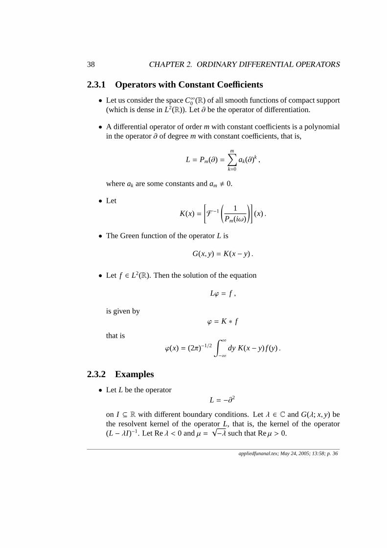
38 CHAPTER 2. ORDINARY DIFFERENTIAL OPERATORS
2.3.1 Operators with Constant Coefficients
• Let us consider the spaceC∞0 (R) of all smooth functions of compact support(which is dense inL2(R)). Let ∂ be the operator of differentiation.
• A differential operator of ordermwith constant coefficients is a polynomialin the operator∂ of degreem with constant coefficients, that is,
L = Pm(∂) =m∑
k=0
ak(∂)k ,
whereak are some constants andam , 0.
• Let
K(x) =
[F −1
(1
Pm(iω)
)](x) .
• The Green function of the operatorL is
G(x, y) = K(x− y) .
• Let f ∈ L2(R). Then the solution of the equation
Lϕ = f ,
is given byϕ = K ∗ f
that is
ϕ(x) = (2π)−1/2
∫ ∞
−∞
dy K(x− y) f (y) .
2.3.2 Examples
• Let L be the operatorL = −∂2
on I ⊆ R with different boundary conditions. Letλ ∈ C andG(λ; x, y) bethe resolvent kernel of the operatorL, that is, the kernel of the operator(L − λI )−1. Let Reλ < 0 andµ =
√−λ such that Reµ > 0.
appliedfunanal.tex; May 24, 2005; 13:58; p. 36
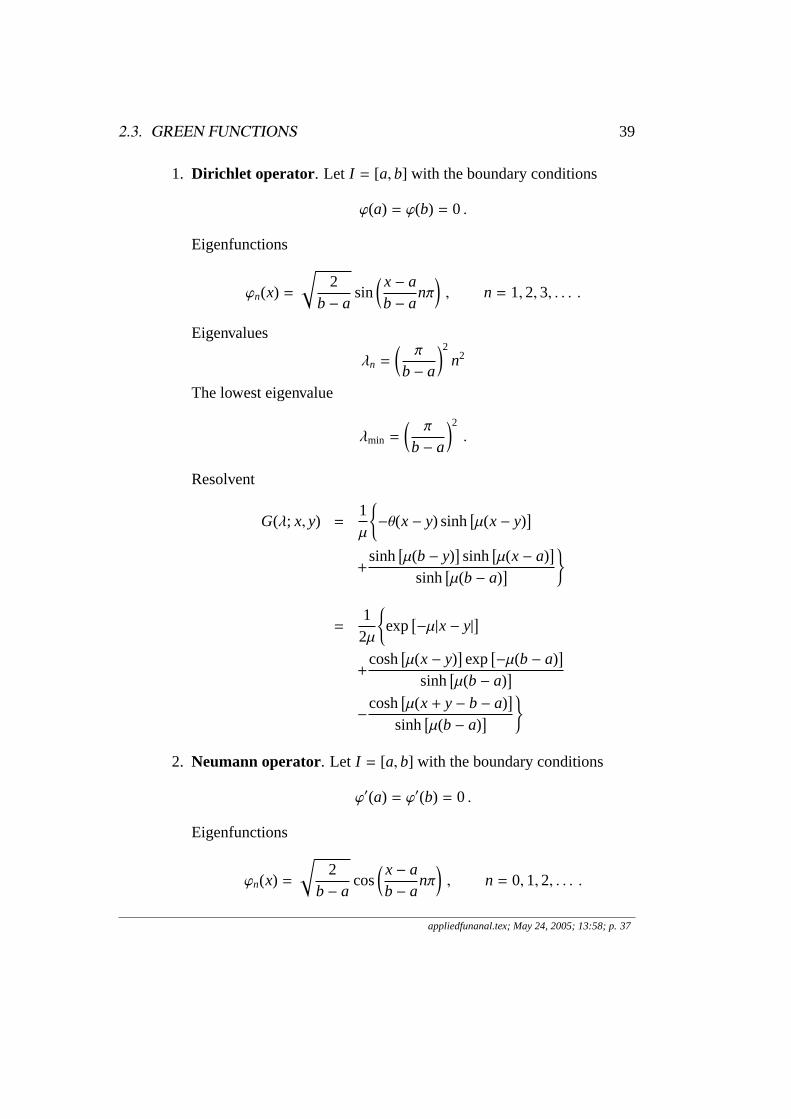
2.3. GREEN FUNCTIONS 39
1. Dirichlet operator . Let I = [a,b] with the boundary conditions
ϕ(a) = ϕ(b) = 0 .
Eigenfunctions
ϕn(x) =
√2
b− asin
( x− ab− a
nπ), n = 1,2,3, . . . .
Eigenvalues
λn =
(π
b− a
)2
n2
The lowest eigenvalue
λmin =
(π
b− a
)2
.
Resolvent
G(λ; x, y) =1µ
−θ(x− y) sinh
[µ(x− y)
]+
sinh[µ(b− y)
]sinh
[µ(x− a)
]sinh
[µ(b− a)
]
=12µ
exp
[−µ|x− y|
]+
cosh[µ(x− y)
]exp
[−µ(b− a)
]sinh
[µ(b− a)
]−
cosh[µ(x+ y− b− a)
]sinh
[µ(b− a)
] 2. Neumann operator. Let I = [a,b] with the boundary conditions
ϕ′(a) = ϕ′(b) = 0 .
Eigenfunctions
ϕn(x) =
√2
b− acos
( x− ab− a
nπ), n = 0,1,2, . . . .
appliedfunanal.tex; May 24, 2005; 13:58; p. 37
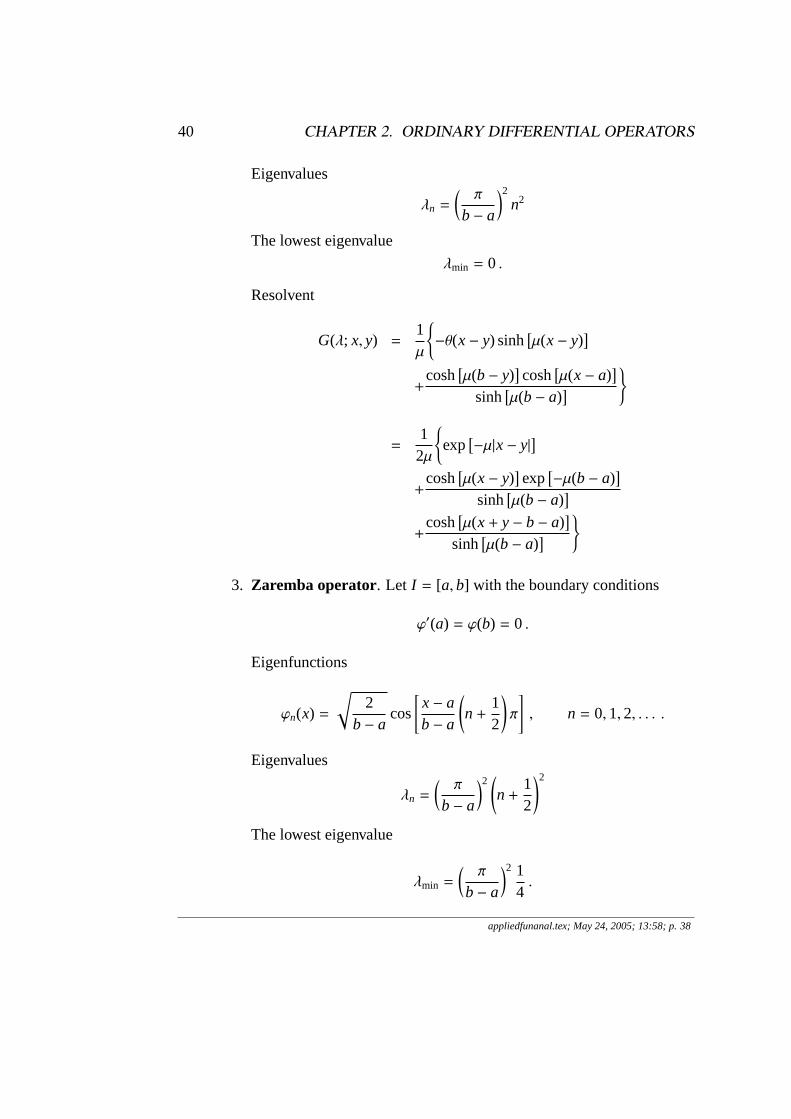
40 CHAPTER 2. ORDINARY DIFFERENTIAL OPERATORS
Eigenvalues
λn =
(π
b− a
)2
n2
The lowest eigenvalue
λmin = 0 .
Resolvent
G(λ; x, y) =1µ
−θ(x− y) sinh
[µ(x− y)
]+
cosh[µ(b− y)
]cosh
[µ(x− a)
]sinh
[µ(b− a)
]
=12µ
exp
[−µ|x− y|
]+
cosh[µ(x− y)
]exp
[−µ(b− a)
]sinh
[µ(b− a)
]+
cosh[µ(x+ y− b− a)
]sinh
[µ(b− a)
]
3. Zaremba operator. Let I = [a,b] with the boundary conditions
ϕ′(a) = ϕ(b) = 0 .
Eigenfunctions
ϕn(x) =
√2
b− acos
[x− ab− a
(n+
12
)π
], n = 0,1,2, . . . .
Eigenvalues
λn =
(π
b− a
)2(n+
12
)2
The lowest eigenvalue
λmin =
(π
b− a
)2 14.
appliedfunanal.tex; May 24, 2005; 13:58; p. 38

2.3. GREEN FUNCTIONS 41
Resolvent
G(λ; x, y) =1µ
−θ(x− y) sinh
[µ(x− y)
]+
sinh[µ(b− y)
]cosh
[µ(x− a)
]cosh
[µ(b− a)
]
=12µ
exp
[−µ|x− y|
]−
cosh[µ(x− y)
]exp
[−µ(b− a)
]cosh
[µ(b− a)
]−
sinh[µ(x+ y− b− a)
]cosh
[µ(b− a)
] 4. Laplacian on the real line. Let I = Rwith the boundedness condition
at±∞. Spectrum is [0,∞) with no discrete eigenvalues.Resolvent
G(λ; x, y) =12µ
exp[−µ|x− y|
]5. Dirichlet operator on half-line . Let I = R+ with the boundedness
condition at∞ and Dirichlet condition at zero
ϕ(0) = 0 .
Spectrum is [0,∞) with no discrete eigenvalues.Resolvent
G(λ; x, y) =12µ
exp
[−µ|x− y|
]− exp
[−µ(x+ y)
].
6. Neumann operator on half-line. Let I = R+ with the boundednesscondition at∞ and Neumann condition at zero
ϕ′(0) = 0 .
Spectrum is [0,∞) with no discrete eigenvalues.Resolvent
G(λ; x, y) =12µ
exp
[−µ|x− y|
]+ exp
[−µ(x+ y)
].
appliedfunanal.tex; May 24, 2005; 13:58; p. 39

42 CHAPTER 2. ORDINARY DIFFERENTIAL OPERATORS
2.3.3 Homework
• Exercises:
appliedfunanal.tex; May 24, 2005; 13:58; p. 40
Chapter 3
Distributions and PartialDifferential Equations
3.1 Distributions
• Let x = (xµ) = (x1, . . . , xn) be Cartesian coordinates inRn.
• We consider the spaceC∞(Rn) of smooth functions onRn.
• The operators
Dµ = ∂µ =∂
∂xµ
are partial differential operators acting on smooth functions.
• Letα = (α1, . . . , αn), αi ≥ 0 ,
be a multiindex withαi be nonnegative integers and
|α| = α1 + · · ·αn
be the norm (length) of the multiindexα.
• We denote by
Dα = Dα11 · · ·D
αnn =
∂|α|
∂(x1)α1 · · · ∂(xn)αn
a partial differential operator of order|α|.
43
44CHAPTER 3. DISTRIBUTIONS AND PARTIAL DIFFERENTIAL EQUATIONS
• Let aα = aα1...αn be smooth functions onRn. Then the operator
L =∑|α|≤m
aα(x)Dα
is a linear partial di fferential operator of order m.
• Alternatively, any differential operator of ordermcan be written in the form
L =m∑
k=0
aµ1...µk∂µ1 · · · ∂µk ,
whereaµ1...µk are smooth functions overRn and a summation over repeatedindices is understood.
• The formal adjoint of the operatorL with respect to theL2 inner productwith unit weight is
L∗ =∑|α|≤m
(−1)|α|Dαaα .
• Let ξ = (ξµ) = (ξ1, . . . , ξn) be a vector inRn and
ξα = ξα11 · · · ξ
αnn .
Thesymbolof the operatorL is a function onRn × Rn defined by
σ(L; x, ξ) =∑|α|≤m
aα(x)ξα .
• Theprincipal part of the operatorL is
Lp =∑|α|=m
aα(x)Dα .
• Theprincipal symbol of the operatorL is a function onRn×Rn defined by
σp(L; x, ξ) =∑|α|=m
aα(x)ξα .
appliedfunanal.tex; May 24, 2005; 13:58; p. 41
3.1. DISTRIBUTIONS 45
• Idea of distributions. Let g be a given function. Consider the differentialequation
L f = g .
Let us multiply it by a “nice” functionϕ. Then
(L f , ϕ) = (g, ϕ)
or( f , L∗ϕ) = (g, ϕ) .
A function f may satisfy this equationwithout being m times differentiable!
• Notice that if f ∈ C(Rn) is continuous andϕ ∈ C∞0 (R) is smooth withcompact support, then the equation (f , ϕ) = 0 implies f = 0.
•
Definition 3.1.1 (Test Functions.)A test function is a smooth func-tion with compact support inRn. The space of the test functions isdenoted byD(Rn). That isD(Rn) = C∞0 (Rn).
• Example. Let |x| =√
(x1)2 + · · · + (xn)2. Then
ϕ(x) =
exp
(1
|x|2 − 1
), if |x| < 1
0, if |x| ≥ 1
is a test function.
•
Theorem 3.1.1 The spaceD(Rn) is a vector space. Letϕ, ψ ∈ D(Rn),f ∈ C∞(Rn) and A : Rn → Rn be an affine transformation (that is anondegenerate linear transformation). Then
1. fϕ ∈ D(Rn), that isD(Rn) is a module over C∞(Rn),
2. ϕ A ∈ D(Rn), that isD(Rn) is invariant under the action of thegroup of affine transformations,
3. ϕ ∗ ψ ∈ D(Rn), that isD(Rn) is closed under the convolution.
Proof: Exercise.
appliedfunanal.tex; May 24, 2005; 13:58; p. 42
46CHAPTER 3. DISTRIBUTIONS AND PARTIAL DIFFERENTIAL EQUATIONS
•
Definition 3.1.2 (Convergence of Test Functions.)Let ϕ ∈ D(Rn) bea test function and(ϕn) be a sequence of test functions. Then the se-quence(ϕn) converges toϕ inD(Rn) if:
1. there is a compact set B⊂ Rn (independent of n) such that allϕn
vanish outside B, that is
∞⋃n=1
suppϕn ⊂ B ,
2. for anyαDαϕn→ Dαϕ
uniformly onRn.
• Notation. Convergence inD(Rn) is denoted by
ϕnD→ ϕ
• Examples.
•
Theorem 3.1.2 Let (ϕn) and (ψn) be sequences inD(Rn) andϕ, psi ∈D(Rn) be such that
ϕnD→ ϕ and ψn
D→ ψ .
let a,b ∈ C, f ∈ C∞(Rn), A be an affine transformation ofRn, andα bea multiindex. Then:
1. aϕn + bψnD→ aϕ + bψ,
2. fϕnD→ fϕ,
3. ϕn AD→ ϕ A,
4. DαϕnD→ Dαϕ.
Proof: Exercise.
appliedfunanal.tex; May 24, 2005; 13:58; p. 43

3.1. DISTRIBUTIONS 47
•
Definition 3.1.3 A distribution (or a generalized function) F on Rn
is a continuous linear functional onD(Rn).
That is, a distribution F onRn is a mapping F: Rn→ C such that
1. F(aϕ + bψ) = aF(ϕ) + bF(ψ) for any a,b ∈ C andϕ, ψ ∈ D(Rn),
2. F(ϕn)→ F(ϕ) in C for any sequence(ϕn) inD(Rn) converging to
ϕ ∈ D(Rn) inD(Rn), i.e.ϕnD→ ϕ.
• Notation. The space of all distributions is denoted byD′(Rn).
The action of the distributionF on a test functionϕ is denoted by
F(ϕ) = 〈F, ϕ〉 .
• Every locally integrable functionf can be identified with a distributionFby
〈F, ϕ, 〉 = (ϕ, f ) .
•
Definition 3.1.4 (Regular and Singular Distributions.) A distribu-tion F ∈ D′(Rn) is called regular if there is a locally integrablefunction f such that for any test functionϕ ∈ D(Rn),
〈F, ϕ〉 = (ϕ, f ) .
A distribution which is not regular is calledsingular.
• Heaviside distribution. Let Ω ⊂ Rn be an open set inRn andχΩ be thecharacteristic function ofΩ. The Heaviside distribution H is a regulardistribution defined by
〈F, ϕ〉 = (ϕ, χΩ) =∫Ω
ϕ .
If Ω = (0,∞) × · · · × (0,∞), then the distribution
〈H, ϕ〉 =∫ ∞
0· · ·
∫ ∞
0dx1 · · · dxnϕ(x) .
• Dirac distribution δ is a singular distribution defined by
〈δ, ϕ〉 = ϕ(0) .
appliedfunanal.tex; May 24, 2005; 13:58; p. 44
48CHAPTER 3. DISTRIBUTIONS AND PARTIAL DIFFERENTIAL EQUATIONS
• Let A be an operator defined on test functions, i.e. onD(Rn). We can extendit to distributions, i.e. toD′(Rn),by
〈AF, ϕ〉 = 〈F,A∗ϕ〉 .
•
Definition 3.1.5 (Derivative of Distributions) The derivative∂µF of adistribution F ∈ D′(Rn) is defined by
〈∂µF, ϕ〉 = 〈F, (−∂µ)ϕ〉 .
More generally,〈DαF, ϕ〉 = 〈F, (−1)|α|Dαϕ〉 ,
and for any differential operator L
〈LF, ϕ〉 = 〈F, L∗ϕ〉 .
•Theorem 3.1.3 Let F be a distribution and L be a differential operatorwith smooth coefficients. Then LF is a distribution.
Proof: Prove the linearity and continuity ofDαF.
• Example.〈Dαδ, ϕ〉 = (−1)|α|Dαϕ(0) .
•
Definition 3.1.6 (Weak Distributional Convergence.)A sequence ofdistributions (Fn) in D′(Rn) converges to a distribution F∈ D′(Rn)if for everyϕ ∈ D(Rn)
〈Fn, ϕ〉 → 〈F, ϕ〉 .
This convergence is called weak distributional convergence.
• Examples.
1. Let f , fn ∈ C(Rn) and fn→ f uniformly on any compact subset ofRn.Let F, Fn be the corresponding regular distributions. ThenFn→ F.
2. Let f , fn ∈ L1(Rn) and fn → f in L1(Rn). Let F, Fn be the correspond-ing regular distributions. ThenFn→ F.
appliedfunanal.tex; May 24, 2005; 13:58; p. 45
3.1. DISTRIBUTIONS 49
• Terminology. If a sequence of regular distributionsFn corresponding to asequence of functionsfn converges to a distributionF, then we say that thesequence of functionsfn converges in the distributional sense (or con-verges distributionally) to the distributionF.
• Example. Sequences of functions converging distributionally to the Diracdistribution. Letn ∈ N.
1.
fn(x) =1π
n1+ n2x2
.
2.fn(x) =
n√π
e−n2x2.
3.
fn(x) =sin(nx)πx
.
•
Theorem 3.1.4 Let (Fn) be a sequence inD′(Rn) converging to F∈D′(Rn), that is Fn→ F. Then for any multiindexα
DαFn→ DαF .
Proof: Note that
〈DαFn, ϕ〉 → (−1)|α|〈F,Dαϕ〉 = 〈DαF, ϕ〉 .
•Definition 3.1.7 (Antiderivative of Distributions.) Let F,G ∈ D′(R)be distributions onR. Then G is ananti-derivative of F if G′ = F.
• Theorem 3.1.5 Every distribution onR has an anti-derivative.
Proof:
1. Letϕ0 ∈ D(R) be a test function such that∫ϕ0 = 1 .
appliedfunanal.tex; May 24, 2005; 13:58; p. 46
50CHAPTER 3. DISTRIBUTIONS AND PARTIAL DIFFERENTIAL EQUATIONS
2. Letϕ ∈ D(R) and
K =∫
ϕ .
Then there is a decomposition
ϕ = Kϕ0 + ϕ1 ,
where ∫ϕ1 = 0 .
3. Let
ψ(x) =∫ x
−∞
dt ϕ1(t) .
Let F,G ∈ D′(R) such that
〈G, ϕ〉 = KC0 − 〈F, ψ〉 ,
whereC0 is a constant. Then
G′ = F .
•Theorem 3.1.6 Let F ∈ ′(R) be a distribution onR. If F ′ = 0, then Fis a constant function.
Proof:
1. Letϕ = Kϕ0 + ϕ1 ∈ D(R) ,
where ∫ϕ0 = 1 ,
∫ϕ1 = 0 ,
and
K =∫
ϕ .
Let
ψ(x) =∫ x
−∞
dt ϕ1(t) .
appliedfunanal.tex; May 24, 2005; 13:58; p. 47
3.1. DISTRIBUTIONS 51
2. Then〈F, ϕ1〉 = 〈F, ψ
′〉 = −〈F′, ψ〉 = 0 .
3. Therefore,
〈F, ϕ〉 = K〈F, ϕ0〉 =
∫Cϕ ,
whereC = 〈F, ϕ0〉.
4. Thus,F is a regular distribution generated by the constant functionC.
•
Definition 3.1.8 (The SpaceD(Ω)) . Test Functions on an Open SetΩ of Rn. LetΩ ⊂ Rn be an open set inRn. The spaceD(Ω) of testfunctions is the space C∞0 (Ω) of smooth functions with compact supportcontained inΩ.
•
Definition 3.1.9 (Convergence inD(Ω)) . Let ϕ ∈ D(Ω) be a testfunction and(ϕn) be a sequence of test functions onΩ. Then the se-quence(ϕn) converges toϕ inD(Ω), denotedϕn→ ϕ inD(Ω), if:
1. there is a compact set B⊂ Ω (independent of n) such that allϕn
vanish outside B, that is
∞⋃n=1
suppϕn ⊂ B ,
2. for anyαDαϕn→ Dαϕ
uniformly onΩ.
•
Definition 3.1.10 (The SpaceD′(Ω)) . Distributions on an Open SetΩ of Rn. The spaceD′(Ω) of distributions is the space of all continuouslinear functionals onD(Ω).
3.1.1 Homework
• Exercises:
appliedfunanal.tex; May 24, 2005; 13:58; p. 48
52CHAPTER 3. DISTRIBUTIONS AND PARTIAL DIFFERENTIAL EQUATIONS
3.2 Fundamental Solutions of Partial Differential Equa-tions
3.2.1 Boundary Value Problems
•
Definition 3.2.1 Let m∈ N and let L : C∞(Rn) → C∞(Rn) be a differ-entiable operator of order m with smooth coefficients acting on smoothfunctions onRn.
1. Let f ∈ Cm(Rn) be a m times differentiable function onRn. Thena function u∈ Cm(Rn) such that
(Lu)(x) = f (x) , for all x ∈ Rn
is theclassical solutionof the equation Lu= f .
2. Let f be a function or a distribution onRn. Then a function u onRn such that
(u, L∗ϕ) = ( f , ϕ)
for every test functionϕ ∈ D(Rn) is the weak solution of theequation Lu= f .
3. Let f ∈ D′(Rn) be a distribution onRn. Then a distribution u∈D′(Rn) such that
Lu = f
is thedistributional solution of the equation Lu= f .
• Examples.
•
Definition 3.2.2 Let L be a differential operator. Afundamental solu-tion G of L is a distributional solution of the equation
LG = δ .
• A fundamental solution is not unique.
• Let f be a function,G be a fundamental solution of the operatorL andu = f ∗G. Thenu satisfies the equation
Lu = f .
appliedfunanal.tex; May 24, 2005; 13:58; p. 49
3.2. FUNDAMENTAL SOLUTIONS OF PARTIAL DIFFERENTIAL EQUATIONS53
• The Heaviside distribution is the fundamental solution of the operatorL =∂x.
• LetΩ ⊂ Rn be a bounded open set inRn with a smooth boundary∂Ω. Let Nbe the outward pointing unit normal toΩ and∇N be the normal derivative.Let f be a function onRn. Thehomogeneous boundary value problemisthe equation
Lu = f in Ω ,
with the boundary conditions
Bu∣∣∣∂Ω= 0 ,
whereB is the boundary operator. One considers the following boundaryoperators:
Dirichlet : B = 1 ,
Neumann : B = ∇N ,
Robin : B = ∇N + g ,
whereg is a smooth function on∂Ω.
•
Definition 3.2.3 A Green function G of the boundary value problem(L, B) is a fundamental solution of the operator L that satisfies the ho-mogeneous boundary conditions.
3.2.2 Equations of Mathematical Physics
• Let x ∈ Rn be the space coordinates andt ∈ R be the time.
• Let gµν be the components of the metric tensor in some local coordinates.TheLaplace Operator (or Laplacian) is a second-order partial differentialoperator acting on smooth functions of the form
∆ = g−1/2∂µg1/2gµν∂ν .
In Cartesian coordinates inRn the Laplacian has the form
∆ = δµν∂µ∂ν =
n∑µ=1
∂2µ .
appliedfunanal.tex; May 24, 2005; 13:58; p. 50
54CHAPTER 3. DISTRIBUTIONS AND PARTIAL DIFFERENTIAL EQUATIONS
• TheD’Alambert Operator (or D’Alambertian ) is a second-order partialdifferential operator
= −∂2t + ∆ .
• Laplace Equation∆u = 0 .
• Poisson Equation∆u = f .
• Wave Equation−u = (∂2
t − ∆)u = f .
Homogeneous wave equation
u = (∂2t − ∆)u = 0 .
• Heat Equation(∂t − ∆)u = f .
Homogeneous heat equation
(∂t − ∆)u = 0 .
• Telegrapher Equation
(∂2t + 2∂t − ∆ + q)u = 0 ,
whereq is a constant.
• Helmholtz Equation(k2 + ∆)u = f ,
Homogeneous Helmholtz equation
(k2 + ∆)u = 0 ,
wherek is a constant.
• Biharmonic Wave Equation.
(∂2t + ∆
2)u = 0 .
appliedfunanal.tex; May 24, 2005; 13:58; p. 51
3.2. FUNDAMENTAL SOLUTIONS OF PARTIAL DIFFERENTIAL EQUATIONS55
• Biharmonic Equation.∆2u = 0 .
• Schrodinger Equation.
(i∂t − ∆ + V)u = 0 ,
whereV is a function onRn.
• Stationary Schrodinger Equation.
(−∆ + V − E)u = 0 ,
whereE is a constant.
• Klein-Gordon Equation .
(− +m2)u = (∂2t − ∆ +m2)u = 0 ,
wherem is a constant.
3.2.3 Green’s Formulas
• LetΩ be a bounded open set inRn with a smooth boundary∂Ω. Let ∂Ω beparametrized by
xµ = xµ(x) ,
wherexi, i = 1, . . . ,n− 1, are the parameters (local coordinates on∂Ω).
• Let gµν be the metric inΩ (equal toδµν in Cartesian coordinates). Theinduced metric ˆgi j on∂Ω is defined by
gi j (x) = gµν(x(x))∂xµ
∂xi
∂xν
∂x j.
• The volume elements inΩ and∂Ω are defined by
dvol(x) = dx√
g(x) , dvol(x) = dx√
g(x)
whereg = detgµν , g = detgi j .
appliedfunanal.tex; May 24, 2005; 13:58; p. 52
56CHAPTER 3. DISTRIBUTIONS AND PARTIAL DIFFERENTIAL EQUATIONS
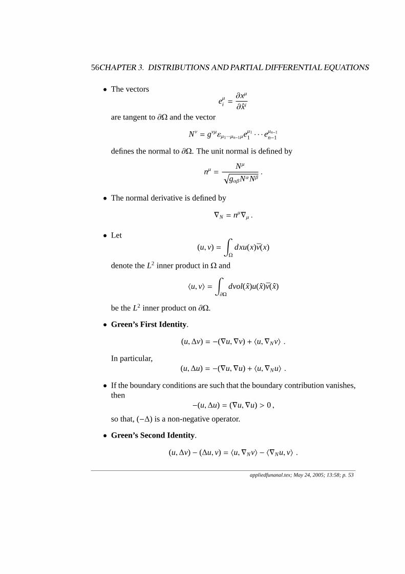
• The vectors
eµi =∂xµ
∂xi
are tangent to∂Ω and the vector
Nν = gνµεµ1···µn−1µeµ1
1 · · · eµn−1
n−1
defines the normal to∂Ω. The unit normal is defined by
nµ =Nµ√
gαβNαNβ.
• The normal derivative is defined by
∇N = nµ∇µ .
• Let
(u, v) =∫Ω
dxu(x)v(x)
denote theL2 inner product inΩ and
〈u, v〉 =∫∂Ω
dvol(x)u(x)v(x)
be theL2 inner product on∂Ω.
• Green’s First Identity .
(u,∆v) = −(∇u,∇v) + 〈u,∇Nv〉 .
In particular,(u,∆u) = −(∇u,∇u) + 〈u,∇Nu〉 .
• If the boundary conditions are such that the boundary contribution vanishes,then
−(u,∆u) = (∇u,∇u) > 0 ,
so that, (−∆) is a non-negative operator.
• Green’s Second Identity.
(u,∆v) − (∆u, v) = 〈u,∇Nv〉 − 〈∇Nu, v〉 .
appliedfunanal.tex; May 24, 2005; 13:58; p. 53
3.2. FUNDAMENTAL SOLUTIONS OF PARTIAL DIFFERENTIAL EQUATIONS57
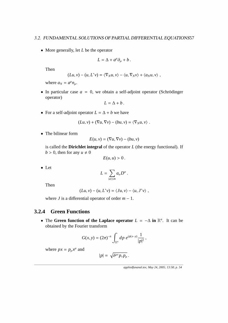
• More generally, letL be the operator
L = ∆ + aµ∂µ + b .
Then(Lu, v) − (u, L∗v) = 〈∇Nu, v〉 − 〈u,∇Nv〉 + 〈aNu, v〉 ,
whereaN = aµnµ.
• In particular casea = 0, we obtain a self-adjoint operator (Schrodingeroperator)
L = ∆ + b .
• For a self-adjoint operatorL = ∆ + b we have
(Lu, v) + (∇u,∇v) − (bu, v) = 〈∇Nu, v〉 .
• The bilinear formE(u, v) = (∇u,∇v) − (bu, v)
is called theDirichlet integral of the operatorL (the energy functional). Ifb > 0, then for anyu , 0
E(u,u) > 0 .
• LetL =
∑|α|≤m
aαDα .
Then(Lu, v) − (u, L∗v) = 〈Ju, v〉 − 〈u, J∗v〉 ,
whereJ is a differential operator of orderm− 1.
3.2.4 Green Functions
• The Green function of the Laplace operator L = −∆ in Rn. It can beobtained by the Fourier transform
G(x, y) = (2π)−n
∫Rn
dp eip(x−y) 1|p|2
,
wherepx= pµxµ and|p| =
√δµνpνpµ .
appliedfunanal.tex; May 24, 2005; 13:58; p. 54
58CHAPTER 3. DISTRIBUTIONS AND PARTIAL DIFFERENTIAL EQUATIONS
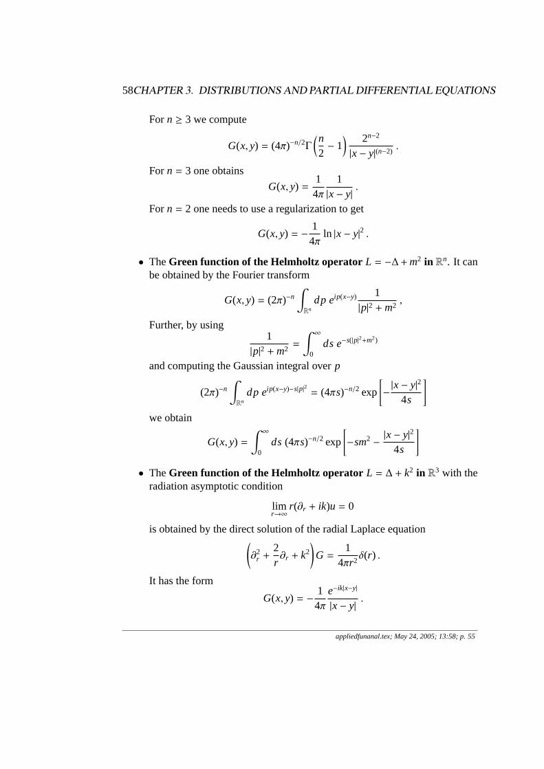
For n ≥ 3 we compute
G(x, y) = (4π)−n/2Γ
(n2− 1
) 2n−2
|x− y|(n−2).
For n = 3 one obtains
G(x, y) =14π
1|x− y|
.
For n = 2 one needs to use a regularization to get
G(x, y) = −14π
ln |x− y|2 .
• TheGreen function of the Helmholtz operator L = −∆+m2 in Rn. It canbe obtained by the Fourier transform
G(x, y) = (2π)−n
∫Rn
dp eip(x−y) 1|p|2 +m2
,
Further, by using1
|p|2 +m2=
∫ ∞
0ds e−s(|p|2+m2)
and computing the Gaussian integral overp
(2π)−n
∫Rn
dp eip(x−y)−s|p|2 = (4πs)−n/2 exp
[−|x− y|2
4s
]we obtain
G(x, y) =∫ ∞
0ds (4πs)−n/2 exp
[−sm2 −
|x− y|2
4s
]• TheGreen function of the Helmholtz operator L = ∆ + k2 in R3 with the
radiation asymptotic condition
limr→∞
r(∂r + ik)u = 0
is obtained by the direct solution of the radial Laplace equation(∂2
r +2r∂r + k2
)G =
14πr2
δ(r) .
It has the form
G(x, y) = −14π
e−ik|x−y|
|x− y|.
appliedfunanal.tex; May 24, 2005; 13:58; p. 55
3.2. FUNDAMENTAL SOLUTIONS OF PARTIAL DIFFERENTIAL EQUATIONS59
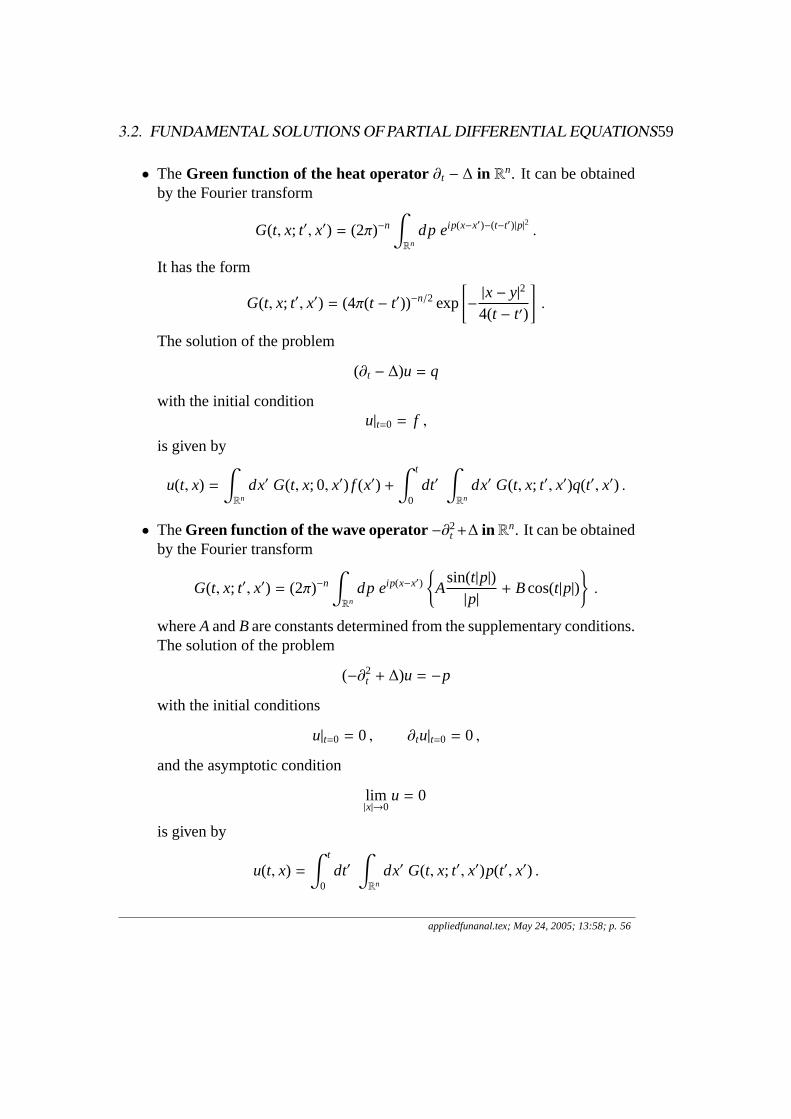
• TheGreen function of the heat operator∂t − ∆ in Rn. It can be obtainedby the Fourier transform
G(t, x; t′, x′) = (2π)−n
∫Rn
dp eip(x−x′)−(t−t′)|p|2 .
It has the form
G(t, x; t′, x′) = (4π(t − t′))−n/2 exp
[−|x− y|2
4(t − t′)
].
The solution of the problem
(∂t − ∆)u = q
with the initial conditionu|t=0 = f ,
is given by
u(t, x) =∫Rn
dx′ G(t, x; 0, x′) f (x′) +∫ t
0dt′
∫Rn
dx′ G(t, x; t′, x′)q(t′, x′) .
• TheGreen function of the wave operator−∂2t +∆ in Rn. It can be obtained
by the Fourier transform
G(t, x; t′, x′) = (2π)−n
∫Rn
dp eip(x−x′)
A
sin(t|p|)|p|
+ Bcos(t|p|)
.
whereA andBare constants determined from the supplementary conditions.The solution of the problem
(−∂2t + ∆)u = −p
with the initial conditions
u|t=0 = 0 , ∂tu|t=0 = 0 ,
and the asymptotic condition
lim|x|→0
u = 0
is given by
u(t, x) =∫ t
0dt′
∫Rn
dx′ G(t, x; t′, x′)p(t′, x′) .
appliedfunanal.tex; May 24, 2005; 13:58; p. 56
60CHAPTER 3. DISTRIBUTIONS AND PARTIAL DIFFERENTIAL EQUATIONS
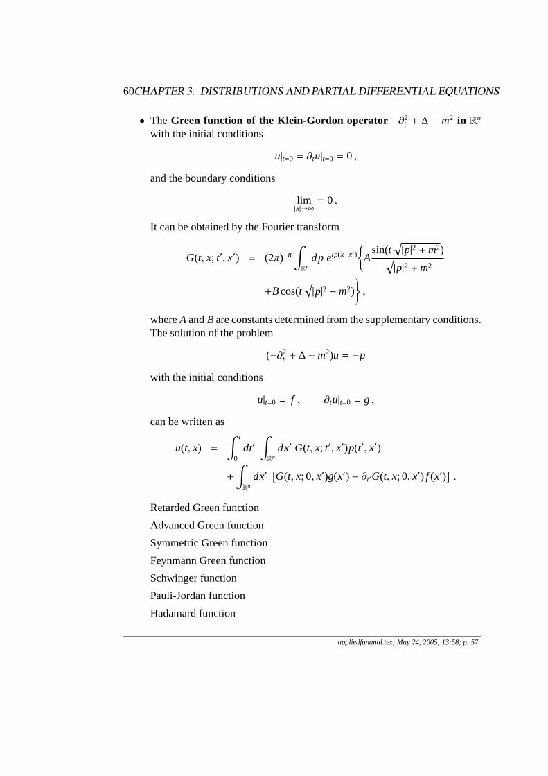
• The Green function of the Klein-Gordon operator −∂2t + ∆ − m2 in Rn
with the initial conditions
u|t=0 = ∂tu|t=0 = 0 ,
and the boundary conditions
lim|x|→∞
= 0 .
It can be obtained by the Fourier transform
G(t, x; t′, x′) = (2π)−n
∫Rn
dp eip(x−x′)
A
sin(t√|p|2 +m2)√|p|2 +m2
+Bcos(t√|p|2 +m2)
,
whereA andBare constants determined from the supplementary conditions.The solution of the problem
(−∂2t + ∆ −m2)u = −p
with the initial conditions
u|t=0 = f , ∂tu|t=0 = g ,
can be written as
u(t, x) =∫ t
0dt′
∫Rn
dx′ G(t, x; t′, x′)p(t′, x′)
+
∫Rn
dx′[G(t, x; 0, x′)g(x′) − ∂t′G(t, x; 0, x′) f (x′)
].
Retarded Green function
Advanced Green function
Symmetric Green function
Feynmann Green function
Schwinger function
Pauli-Jordan function
Hadamard function
appliedfunanal.tex; May 24, 2005; 13:58; p. 57
3.2. FUNDAMENTAL SOLUTIONS OF PARTIAL DIFFERENTIAL EQUATIONS61
3.2.5 Homework
• Exercises: 6.6[27,28,29,32]
appliedfunanal.tex; May 24, 2005; 13:58; p. 58
62CHAPTER 3. DISTRIBUTIONS AND PARTIAL DIFFERENTIAL EQUATIONS
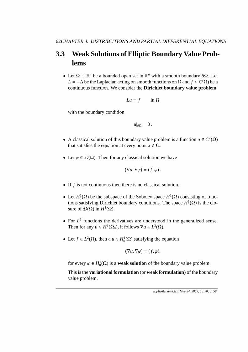
3.3 Weak Solutions of Elliptic Boundary Value Prob-lems
• Let Ω ⊂ Rn be a bounded open set inRn with a smooth boundary∂Ω. LetL = −∆ be the Laplacian acting on smooth functions onΩ and f ∈ C(Ω) be acontinuous function. We consider theDirichlet boundary value problem:
Lu = f in Ω
with the boundary condition
u|∂Ω = 0 .
• A classical solution of this boundary value problem is a functionu ∈ C2(Ω)that satisfies the equation at every pointx ∈ Ω.
• Let ϕ ∈ D(Ω). Then for any classical solution we have
(∇u,∇ϕ) = ( f , ϕ) .
• If f is not continuous then there is no classical solution.
• Let H10(Ω) be the subspace of the Sobolev spaceH1(Ω) consisting of func-
tions satisfying Dirichlet boundary conditions. The spaceH10(Ω) is the clo-
sure ofD(Ω) in H1(Ω).
• For L2 functions the derivatives are understood in the generalized sense.Then for anyu ∈ H1(Ω0), it follows ∇u ∈ L2(Ω).
• Let f ∈ L2(Ω), then au ∈ H10(Ω) satisfying the equation
(∇u,∇ϕ) = ( f , ϕ),
for everyϕ ∈ H10(Ω) is aweak solutionof the boundary value problem.
This is thevariational formulation (or weak formulation) of the boundaryvalue problem.
appliedfunanal.tex; May 24, 2005; 13:58; p. 59
3.3. WEAK SOLUTIONS OF ELLIPTIC BOUNDARY VALUE PROBLEMS63
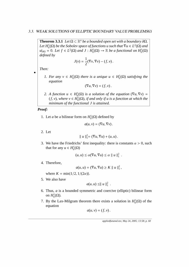
•
Theorem 3.3.1 LetΩ ⊂ Rn be a bounded open set with a boundary∂Ω.Let H1
0(Ω) be the Sobolev space of functions u such that∇u ∈ L2(Ω) andu|∂Ω = 0. Let f ∈ L2(Ω) and J : H1
0(Ω) → R be a functional on H10(Ω)defined by
J(v) =12
(∇v,∇v) − ( f , v) .
Then:
1. For any v∈ H10(Ω) there is a unique u∈ H1
0(Ω) satisfying theequation
(∇u,∇v) = ( f , v) .
2. A function u∈ H10(Ω) is a solution of the equation(∇u,∇v) =
( f , v), where v∈ H10(Ω), if and only if u is a function at which the
minimum of the functional J is attained.
Proof:
1. Leta be a bilinear form onH10(Ω) defined by
a(u, v) = (∇u,∇v) .
2. Let‖ u ‖21= (∇u,∇u) + (u,u) .
3. We have the Friedrichs’ first inequality: there is constantsα > 0, suchthat for anyu ∈ H1
0(Ω)
(u,u) ≤ α(∇u,∇u) ≤ α ‖ u ‖21 .
4. Therefore,a(u,u) = (∇u,∇u) ≥ K ‖ u ‖21 ,
whereK = min1/2,1/(2α).
5. We also havea(u,u) ≤‖ u ‖21 .
6. Thus,a is a bounded symmetric and coercive (elliptic) bilinear formon H1
0(Ω).
7. By the Lax-Milgram theorem there exists a solution inH10(Ω) of the
equationa(u, v) = ( f , v) .
appliedfunanal.tex; May 24, 2005; 13:58; p. 60
64CHAPTER 3. DISTRIBUTIONS AND PARTIAL DIFFERENTIAL EQUATIONS
• Neumann Boundary Value Problem. Let b > 0 be a positive constant andL = −∆ + b. The Neumann boundary value problem is the problem
Lu = f in Ω
with the boundary condition
∇Nu|∂Ω = 0 .
Every classical solutionu ∈ H1(Ω) satisfies the equation
(∇u,∇v) + (bu, v) = ( f , v)
for everyv ∈ H1(Ω).
• Let f ∈ L2(Ω). A weak solution of the Neumann boundary value problemis au ∈ H1(Ω) satisfying the equation
(∇u,∇v) + (bu, v) = ( f , v)
for everyv ∈ H1(Ω).
• Let a be the bilinear form onH1(Ω) defined by
a(u, v) = (∇u,∇v) + (bu, v) .
• We estimatea(u, v) ≤ M ‖ u ‖ ‖ v ‖ ,
whereM = max1,b.
• So,a is continuous and coercive bilinear form inH1(Ω).
• So, by Lax-Milgram theorem there exists a unique solutionu ∈ H1(Ω) sat-isfying the equation
a(u, v) = ( f , v)
for all v ∈ H1(Ω).
appliedfunanal.tex; May 24, 2005; 13:58; p. 61
3.3. WEAK SOLUTIONS OF ELLIPTIC BOUNDARY VALUE PROBLEMS65
• The weak solution of the Neumann boundary value problem minimizes onH1(Ω) the functional
J(v) =12
(∇v,∇v) + (bv, v) − ( f , v) .
• Example.
• General Elliptic Boundary Value Problem. Letaµν,q ∈ C1(Ω) be boundeddifferentiable functions such that
aµν = aνµ .
We will assume for simplicity that the matrixaµν is positive definite andq ≥ 0. LetL be a second-order operator of the form
L = −∂µaµν∂ν + q .
We consider the Dirichlet boundary value problem (L, B) for this operator
Lu = f in Ω
with the boundary condition
u|∂Ω = 0 .
• The operatorL is calleduniformly elliptic if there is a constantC such thatfor anyx ∈ Ω, ξ ∈ Rn, ξ , 0,
|aµν(x)ξµξν| ≥ C|ξ|2 ,
where|ξ| =√δµνξµξν.
• Let f ∈ L2(Ω). A weak solution of the boundary value problem is a functionu ∈ H1
0(Ω) satisfying the equation
(aµν∂µu, ∂νv) + (qu, v) = ( f , v)
for everyv ∈ H10(Ω).
• Every classical solution is a weak solution. Every sufficiently regular weaksolution is a classical solution.
appliedfunanal.tex; May 24, 2005; 13:58; p. 62
66CHAPTER 3. DISTRIBUTIONS AND PARTIAL DIFFERENTIAL EQUATIONS
• Let a be a bilinear form onH10(Ω) defined by
a(u, v) = (aµν∂µu, ∂νv) + (qu, v)
• We estimatea(u,u) ≥ (aµν∂µu, ∂ν) ≥ K(∇u,∇u) .
• Next, we show thata is bounded inH10(Ω).
• Then by Lax-Milgram theorem there exists a unique solutionu ∈ H10(Ω) of
the equationa(u, v) = ( f , v)
for all v ∈ H10(Ω).
• This solution minimizes the functional
J(v) =12
(aµν∂µu, ∂ν) +12
(qv, v) − ( f , v)
on H10(Ω).
3.3.1 Homework
• Exercises: 6.6[23,24,25]
appliedfunanal.tex; May 24, 2005; 13:58; p. 63
Chapter 4
Wavelets and Optimization
4.1 Wavelets
4.1.1 Wavelet Transforms
•
4.1.2 Homework
• Exercises:
67
68 CHAPTER 4. WAVELETS AND OPTIMIZATION
4.2 Calculus of Variations
4.2.1 Gateaux and Frechet Differentials
•
4.2.2 Euler-Lagrange Equations
•
4.2.3 Homework
• Exercises:
appliedfunanal.tex; May 24, 2005; 13:58; p. 64
4.3. DYNAMICAL SYSTEMS 69
4.3 Dynamical Systems
4.3.1 Optimal Control
•
4.3.2 Stability
•
4.3.3 Bifurcations
•
4.3.4 Homework
• Exercises:
appliedfunanal.tex; May 24, 2005; 13:58; p. 65
70 CHAPTER 4. WAVELETS AND OPTIMIZATION
appliedfunanal.tex; May 24, 2005; 13:58; p. 66
Bibliography
[1] L. Debnath and P. Mikusinski,Introduction to Hilbert Spaces with Appli-cations, 2nd Ed., Academic Press, 1999
[2] E. Kreyszig, Introductory Functional Analysis with Applications, Wiley,New York, 1978
[3] M. Reed and B. Simon,Methods of Modern Mathematical Physics, vol. 1,Functional Analysis, Academic Press, New York, 1972
[4] C. DeVito, Functional Analysis and Linear Operator Theory, Addison-Wesley, 1990
[5] E. Zeidler,Applied Functional Analysis, Springer-Verlag, 1995
[6] R. Courant and D. Hilbert,Methods of Mathematical Physics, vol. 1, Inter-science, 1962
[7] R. Richtmeyer,Principles of Advanced Mathematical Physics, Springer-Verlag, 1978
[8] G. Folland,Introduction to partial Differential Equations, 2nd ed., Prince-ton University Press, 1995
[9] I. Stakgold,Green Functions and Boundary Value Problems, Wiley, 1979
[10] M. E. Taylor,Partial Differential Equations, Springer-Verlag, 1996
71

72 Bibliography
appliedfunanal.tex; May 24, 2005; 13:58; p. 67
Notation
Logic
A =⇒ B A impliesBA⇐= B A is implied byBiff if and only ifA⇐⇒ B A impliesB and is implied byB∀x ∈ X for all x in X∃x ∈ X there exists anx in X such that
Sets and Functions (Mappings)
x ∈ X x is an element of the setXx < X x is not inXx ∈ X | P(x) the set of elementsx of the setX obeying the propertyP(x)A ⊂ X A is a subset ofXX \ A complement ofA in XA closure of setAX × Y Cartesian product ofX andYf : X→ Y mapping (function) fromX to Yf (X) range offχA characteristic function of the setA∅ empty setN set of natural numbers (positive integers)Z set of integer numbersQ set of rational numbersR set of real numbersR+ set of positive real numbersC set of complex numbers
73
74 Notation
Vector Spaces
H ⊕G direct sum ofH andGH∗ dual spaceRn vector space ofn-tuples of real numbersCn vector space ofn-tuples of complex numbersl2 space of square summable sequenceslp space of sequences summable withp-th power
Normed Linear Spaces
||x|| norm ofxxn −→ x (strong) convergence
xnw−→ x weak convergence
Function Spaces
suppf support offH ⊗G tensor product ofH andGC0(Rn) space of continuous functions with bounded support inRn
C(Ω) space of continuous functions onΩCk(Ω) space ofk-times differentiable functions onΩC∞(Ω) space of smooth (infinitely diffrentiable) functions onΩD(Rn) space of test functions (Schwartz class)L1(Ω) space of integrable functions onΩL2(Ω) space of square integrable functions onΩLp(Ω) space of functions integrable withp-th power onΩHm(Ω) Sobolev spacesC0(V,Rn) space of continuous vector valued functions with bounded
support inRn
Ck(V,Ω) space ofk-times differentiable vector valued functionsonΩ
C∞(V,Ω) space of smooth vector valued functions onΩ
appliedfunanal.tex; May 24, 2005; 13:58; p. 68
Notation 75
D(V,Rn) space of vector valued test functions (Schwartz class)L1(V,Ω) space of integrable vector valued functions functions
onΩL2(V,Ω) space of square integrable vector valued functions
onΩLp(V,Ω) space of vector valued functions integrable withp-th
power onΩHm(V,Ω) Sobolev spaces of vector valued functions
Linear Operators
Dα differential operatorL(H,G) space of bounded linear transformations fromH to GH∗ = L(H,C) space of bounded linear functionals (dual space)
appliedfunanal.tex; May 24, 2005; 13:58; p. 69

76 Notation
appliedfunanal.tex; May 24, 2005; 13:58; p. 70