Mathematical Methods Notes for Block One
48
MATHEMATICAL METHODS PHY250 Alastair Buckley Sept 2012 Page 1 of 48 PHY250 Physics core for level 2 Autumn Semester 2012 Mathematical Methods Notes for Block One Lecturer: Alastair Buckley http://www.hep.shef.ac.uk/phy226/unit1/phy250_MMblock1.htm Department Of Physics & Astronomy
Transcript of Mathematical Methods Notes for Block One
MATHEMATICAL METHODS PHY250
Alastair Buckley Sept 2012 Page 1 of 48
PHY250 Physics core for level 2 Autumn Semester 2012
Mathematical Methods Notes for Block One Lecturer: Alastair Buckley http://www.hep.shef.ac.uk/phy226/unit1/phy250_MMblock1.htm
DepartmentOf Physics & Astronomy

MATHEMATICAL METHODS PHY250
Alastair Buckley Sept 2012 Page 2 of 48
PHY250 - Mathematical Methods for Physics and Astronomy The Mathematical Methods component of PHY250 is taught in three serial blocks
Block one (8 lectures) Dr Alastair Buckley, E49, [email protected]
1. Revision of algebraic methods 2. Complex numbers and functions 3. Ordinary differential equations 4. Fourier series
Block two Prof. David Mowbray, E14, [email protected]
Fourier integrals & convolution theorem
Block three Dr Vitaly Kudryavtsev, F9b, [email protected]
Partial differential equations Reference material Lectures will impart some knowledge of mathematics but skill can only be obtained by practising. Examples will be given in each lecture but a massive collection of further worked online problems, along with electronic copies of the notes and lecture slides, can be found at http://www.hep.shef.ac.uk/phy226.htm
The notes are pretty complete and can also be found online so there are no compulsory textbooks. Jordan & Smith covers approximately the first half of the course and is recommended. Two other excellent textbooks both of which cover most of the course are:
Mary L. Boas – Mathematical Methods in the Physical Sciences (Wiley) Erwin Kreyszig – Advanced Engineering Mathematics (Academic Press)
The Physics and Astronomy Formula and Data sheet is also a really useful point of reference. You should always have a copy when doing problems or reading the notes.

MATHEMATICAL METHODS PHY250
Alastair Buckley Sept 2012 Page 3 of 48
Content of Lectures 1-8
Topic 1 Brief revision of algebra and functions (lecture 1)
1.1 Multiplying brackets page 4 1.2 Binomial series page 4 1.3 Taylor series page 5 1.4 Why use series approximations page 7 1.5 Trigonometric and Hyperbolic functions page 7 1.6 Exponentials page 8 1.7 Logarithms page 9
Online Problems for topic 1 page 9 Topic 2 Revision of complex numbers (lecture 2)
2.1 Argand diagram: arithmetic operations page 10 2.2 Polar form: geometric operations page 11 2.3 Powers and roots page 13 2.4 Complex exponentials and trig functions page 14 2.5 Differentiation page 14
Online Problems for topic 2 page 15 Topic 3 Ordinary differential equations (ODEs) (lectures 3-5)
3.1 First order ODEs page 16 3.2 Second order ODEs page 18 3.3 Homogenous 2nd order equations page 21 3.4 Inhomogeneous 2nd order equations page 23
Online Problems for topic 3 page 28 Topic 4 Fourier series (Lectures 5-8)
4.1 Introduction to Fourier series page 29 4.2 Why are they useful? page 30 4.3 Towards finding the Fourier coefficients page 31 4.4 Average value of a function page 32 4.5 Orthogonality page 32 4.6 Fourier coefficients – derivation page 33 4.7 Summary of results page 34 4.8 Examples page 35 4.9 Even and Odd functions page 38 4.10 Half range series page 40 4.11 Complex series page 42 4.12 Parseval’s Theorem page 44 4.13 Appendix: Proof of Orthogonality page 45
Online Problems for topic 4 page 46
Summary page 48
MATHEMATICAL METHODS PHY250
Alastair Buckley Sept 2012 Page 4 of 48
Topic 1: Revision of Algebra 1.1 Multiplying Brackets All terms are included, e.g.
)2()2()2)(()( 2222223 yxyxyyxyxxyxyxyxyx +++++=+++=+ Also 2 2( )( )x a x a x a+ − = − You can check these by choosing a simple value for x and y in the above expression. 1.2 Binomial Series (See exam data sheet)
2 3( 1) ( 1)( 2)(1 ) 12! 3!
n nnn n n n nx nx x x xk
− − −+ = + + + + + +
K K, where
( )!
! !n nk n k k
= −
.
• When n is a positive integer we have a finite series: i.e. the series terminates. • When n is negative or non-integer, the series does not terminate. • The series converges for all |x| <1 since x to any power will be smaller than x.
The most useful job of both the binomial and Taylor series is to intelligently approximate an impossibly complicated expression to a few simple terms that pretty well equal the full solution. We do this when we say ‘taking only the first two or three terms’. However we need to apply it correctly.
We can only approximate (1 ) 1nx nx+ ≈ + or 2( 1)(1 ) 12
n n nx nx x−+ ≈ + + when x <<1.
Consider ( )na b+ . This can be rewritten ( ) 1 (1 )n
n n n nba b a a xa
+ = + = +
where x b a=
The intelligent part is to choose a, b such that |a| > |b| so |x| << 1. How many terms you need to use depends on how small x is and on how accurately you need the answer. As a rule of thumb, in most physical applications it is fine to use these approximations for x < 0.1 . Obviously if n is very large you need a correspondingly smaller value of x for rapid convergence.

MATHEMATICAL METHODS PHY250
Alastair Buckley Sept 2012 Page 5 of 48
Example 1.1
(a) Expand 11 x+
in powers of x.
(b) If x = 0.1 and we need accuracy to about 1%, how many terms do we need? Since x3 ~10-3 we would guess we could stop at x2. Let’s check this: The exact answer is 1)1.01( −+ = 0.9090909… . To 1% accuracy this is 0.91. The expansion above gave us:- first term = 1, second term = -x, third term = x2, fourth term = -x3 So 1)1.01( −+ = 1 – 0.1 + (0.12) – (0.13). Yes we can stop after two terms. Example 1.2 Rewrite 15)cos(sin θθ + for small θ using the binomial expansion for the first three terms.
NB. The binomial expansion works for any value of x and n.
It’s just more useful if x <<1

MATHEMATICAL METHODS PHY250
Alastair Buckley Sept 2012 Page 6 of 48
1.3 Taylor Series (also on the exam data sheet)
2( ) ( )( ) ( ) ( )2! !
nnf a f af x a f a f a x x x
n′′
′+ = + + + + +K K where ( )n
nn
x a
d ff adx =
=
Unlike the binomial expansion, the Taylor expansion can also be used for any function that has a derivative. Note that if a = 0 then the Taylor expansion is known as a Maclaurin expansion. The range of x for which there is convergence depends on the function f. But in practice the series is only useful if the first couple of terms give an adequate approximation, which means we need x<<1.
Examples 1.3 and 1.4
1.3 Find the Maclaurin expansion of eαx ?
1.4 Find the first two terms of the expansion of tan( )4
xπ+ .
MATHEMATICAL METHODS PHY250
Alastair Buckley Sept 2012 Page 7 of 48
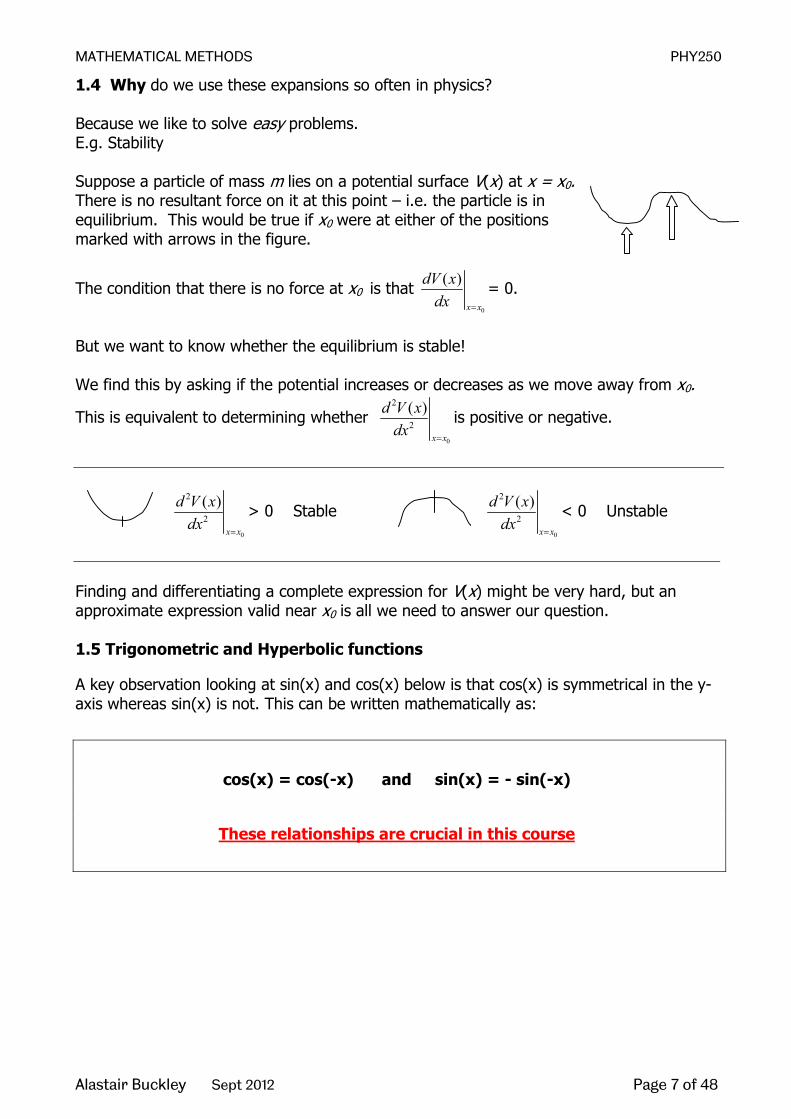
1.4 Why do we use these expansions so often in physics? Because we like to solve easy problems. E.g. Stability Suppose a particle of mass m lies on a potential surface V(x) at x = x0. There is no resultant force on it at this point – i.e. the particle is in equilibrium. This would be true if x0 were at either of the positions marked with arrows in the figure.
The condition that there is no force at x0 is that 0
( )
x x
dV xdx =
= 0.
But we want to know whether the equilibrium is stable! We find this by asking if the potential increases or decreases as we move away from x0.
This is equivalent to determining whether 0
2
2
( )
x x
d V xdx
=
is positive or negative.
0
2
2
( )
x x
d V xdx
=
> 0 Stable 0
2
2
( )
x x
d V xdx
=
< 0 Unstable
Finding and differentiating a complete expression for V(x) might be very hard, but an approximate expression valid near x0 is all we need to answer our question. 1.5 Trigonometric and Hyperbolic functions
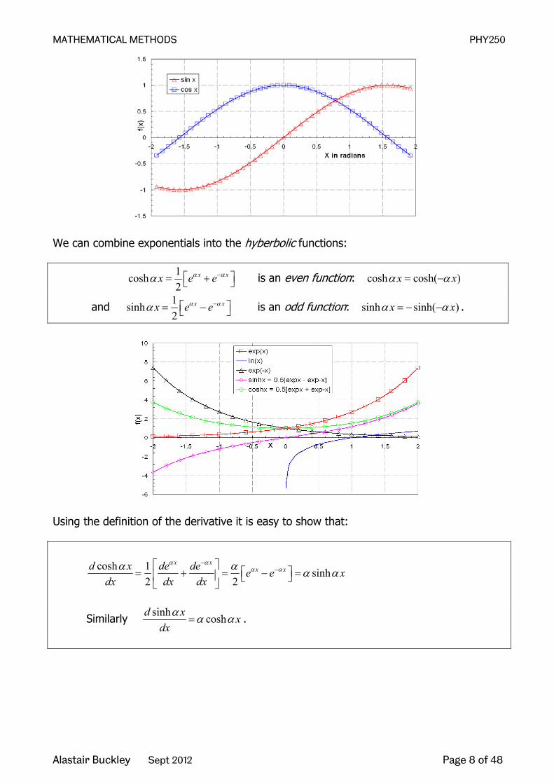
A key observation looking at sin(x) and cos(x) below is that cos(x) is symmetrical in the y-axis whereas sin(x) is not. This can be written mathematically as:
cos(x) = cos(-x) and sin(x) = - sin(-x)
These relationships are crucial in this course
MATHEMATICAL METHODS PHY250
Alastair Buckley Sept 2012 Page 8 of 48
We can combine exponentials into the hyberbolic functions:
1cosh2
x xx e eα αα − = + is an even function: cosh cosh( )x xα α= −
and 1sinh2
x xx e eα αα − = − is an odd function: sinh sinh( )x xα α= − − .
Using the definition of the derivative it is easy to show that:
cosh 1 sinh
2 2
x xx xd x de de e e x
dx dx dx
α αα αα α α α
−−
= + = − =
Similarly sinh coshd x x
dxα α α= .

MATHEMATICAL METHODS PHY250
Alastair Buckley Sept 2012 Page 9 of 48
1.6 Exponentials are powers and so they satisfy: baba eee =+ and ba ee /1=− 1.7 Natural logarithms are defined by
lnxy e x y= = .
We also have that
)/ln(lnln 2121 yyyy =− and )ln(lnln 2121 yyyy =+ We can relate natural logs to those to base 10: Define 10logw y= . This expression means that 10wy = . Take natural logs of both sides:
( ) ( ) lnln ln 10 ln 10ln(10)
w yy w w= = = or ln(10)wy e= .
Online Problems (Topic 1, questions 1-5)
1. Consider (52+3)1.5 . Your calculator will give you an answer of 407.8909 to 4dp. How many terms of a binomial expansion do you need to get within 1% of this?
2. In question 1 what would happen if, by factorising differently, you had chosen to
expand ( ) 5.13
521+ instead of ( ) 5.152
31+ ?
3. Expand ( )5ba + , i) where a and b are 2 and 10 respectively and ii) where a and b are 10 and 2 respectively
4. Expand ( ) 4/122 −
+ ba in powers of b/a up to terms of order b4
5. Expand )1ln( x+ via the Taylor expansion up to the 4th term

MATHEMATICAL METHODS PHY250
Alastair Buckley Sept 2012 Page 10 of 48
6. Topic 2. Complex Numbers
2.1 Argand diagram Let z = a + ib where i2 = - 1 To represent this number on an Argand diagram, plot the point with Cartesian coordinates (a, b). i.e. real numbers run along the x axis and imaginary numbers along the y axis.
The complex conjugate is z* = a – ib (Note: Physicists usually use i, engineers often use j and physicists always denote complex conjugates by z* not z ) By Pythagoras, the length OZ is zbar =+= 22 .
Note that this length is also equal to *zz zz* = 2 2 2( )( ) ( )( )a ib a ib a ib ib a b+ − = + − = + . We also write a2 + b2 = *zz = |z|2 where *z zz= and is called the modulus of z. Example 2.1 Find the modulus of |(2 + 3i)| ?
b
-b
a O
z
z*

MATHEMATICAL METHODS PHY250
Alastair Buckley Sept 2012 Page 11 of 48
2.2 Polar form We can also write
( )φφφ sincos irrez i +== where πφ 20 << r = is again called the modulus, φ is called the argument or phase. For a proof of this relationship see Lecture 2, problem 2 in the online Problems.
Then ( )φφφ sincos* irrez i −== − So 22* reerzz ii == − φφ since 1)( == −− φφφφ iii eee
Clearly φcosra = , φsinrb = and zbar =+= 22
Note that |z| and zz* = |z|2, are always real, whereas z2 = a2+ 2iab - b2 = r2e2iφ ≠ |z|2 is usually complex. In physics we always need to get real answers, hence in quantum mechanics etc. one takes |ψ|2 not ψ2. (In optics and E&M you may sometimes take the real part to get your answer.)
Changing between the forms z = a + ib and z = reiφ
You are strongly advised to first plot the number on an Argand diagram. Without this it is easy to make mistakes about minus signs and angles, etc.! Given z = a + ib, to find the form z = reiφ
Find r using 2 2r a b= + .
Find φ using tan ba
φ = (specifying its sign from the quadrant of the Argand diagram.)
Given z = reiφ, to find the form z = a + ib is easier: a = rcosφ and b = rsinφ . Why do we need both forms? It is easier to add and subtract complex numbers in the form z = a + ib but easier to multiply, divide, take powers and roots when they are in the form z=reiφ. In physics we almost always use the form z = reiφ .
φ r
b
a O
z

MATHEMATICAL METHODS PHY250
Alastair Buckley Sept 2012 Page 12 of 48
Addition and Subtraction If z a ib= + and w c id= + then ( ) ( )z w a c i b d+ = + + + and ( ) ( )z w a c i b d− = − + − . Multiplication and Division For this we always use the form z = r e iφ Let 1
1 1iz r e φ= and 2
2 2iz r e φ=
then 1 2 1 2( )1 2 1 2 1 2
i i iz z r e r e r r eφ φ φ φ+= = i.e. multiply the moduli and add the arguments (phases). Similarly for division:
1 2( )1 2 1 2( / ) ( / ) iz z r r e φ φ−=
i.e. we divide the moduli and subtract the arguments.
Example 2.2 Express (1 + i) ÷ (1 + 1.73i) in polar coordinates?
MATHEMATICAL METHODS PHY250
Alastair Buckley Sept 2012 Page 13 of 48
2.3 Powers and Roots Again we always use the polar form. For a real number power it is straightforward:
n n inz r e φ= i.e. we take the modulus to the nth power and multiply the argument (or phase) by n.
Roots are trickier. We defined φ to lie in the region 0 < φ < 2π. But this will need to be extended if we want to get all the roots of a complex number. We define ( 2 )i pz re φ π+= where p is an integer.
To find an nth root, we need to take n distinct values of p: p = 0, p = 1, p = 2, …, p = n -1.
Then there are n distinct roots to 1 1 ( 2 )n n i p nz r e φ π+= . Example 2.3 : If z = 9 eiπ/3 what is z½ ?
Step 1:
write down z in polars with the 2πp bit added on to the argument. z = 9ei (π/3 + 2πp)
Step 2:
say how many values of p you’ll need and write out the rooted expression here n = 2 so I’ll need 2 values of p; p = 0 and p = 1 z½ = √9 ei ( π/3 + 2πp)/2
Step 3:
Work it out for each value of p: z½ = 3ei (π/3)/2 = 3ei (π/6) for p = 0
z½ = 3ei (π/3 + 2π)/2 = 3ei (π/6 + π) for p = 1
There are your answers but remember that e iφ = (cosφ + isinφ) so e iπ = -1
It’s therefore better to write z½ = 3ei (π/6 + π) = 3ei π/6(eiπ) = -3ei π/6 for p =1, and 3ei (π/6) for p = 0
MATHEMATICAL METHODS PHY250
Alastair Buckley Sept 2012 Page 14 of 48
Example 2.4: If z = 27 eiπ/2 what is z⅓ ?
Step 1: write down z in polars with the 2πp bit added on to the argument.
Step 2: say how many values of p you’ll need and write out the rooted expression
Step 3: Work it out for each value of p
2.4 Exponentials and Trigonometric functions
kxikxeikx sincos += ; and cos sinikxe kx i kx− = −
Rearranging gives 1 1cos ( ); sin ( )2 2
ikx ikx ikx ikxkx e e kx e ei
− −= + = −
This is a key observation…remember this.
2.5 Differentiation of a Complex Exponential
We know kx kxd e kedx
= . Since i is just a constant, we similarly have ikx ikxd e ikedx
=
Note that is much nicer to differentiate exponentials than sines and cosines because we get exactly the same function as we started with, just multiplied by a constant.

MATHEMATICAL METHODS PHY250
Alastair Buckley Sept 2012 Page 15 of 48
Online problems for (Topic 2, questions 1-11)
1. Expand xsinh using the Taylor series up to the 5th power term in x
2. Prove the relationship )sin(cos φφφ irrez i +== using the Taylor expansion
3. Find the modulus of i) i76 + ii) ii
2376
++
and iii) plot )23()76( ii +−+ on an Argand
diagram and give the answer in polar co-ordinates. iv) Express 6/5 πiez = in Cartesian co-ordinates and v) Convert i43 + and i125 + into polar co-ordinates and multiply them.
4. In quantum mechanics we sometimes need to evaluate the modulus squared of
the sum of two complex numbers. If αiAez =1 and βiBez −=2 find 221 || zz +
Manipulate your answer into the form )cos(22 βα −++ ABBA
5. iz 32 += By changing into polar co-ordinates find 18z ?
6. 4/16 πiez = Find 4/1z ?
7. Show that 12
=−+
ibaiba
for any real numbers a and b
8. Find i
9. iz += 1 Find 2/1z
10. Prove titi BeAex )() βαβα −+ += can be written as )cossin( tDtCex t ββα += and
define C and D in terms of A and B
11. Prove that )cossin( tDtCex t ββα += can be written as ))(cos( φβα += tEex t and define φ and E in terms of C and D.

MATHEMATICAL METHODS PHY250
Alastair Buckley Sept 2012 Page 16 of 48
Topic 3. Ordinary Differential Equations (ODE’s)
Most of physics involves the solution of differential equations! The solution of ordinary differential equations (ODEs) was covered in PHY112. ‘Ordinary’ means that all functions are of only one variable. We will revise the theory and explore some examples, especially harmonic oscillators. Later lectures will address the solution of partial differential equations featuring multiple variables.
3.1 First Order ODEs (i.e. 1 variable and no higher than dtdx terms)
Revision of Theory You should be aware of two possible methods for solving 1st order ODEs. Which method you use depends on the equation you are trying to solve.
1. Some equations can be solved by the method of separation of the variables: rearrange the equation so that each side involves only one variable, then integrate both sides.
2. The method of trial solution may be used.
The general solution of a 1st order equation will contain one arbitrary constant; the value of the constant is determined by the boundary conditions, yielding a particular solution.
Example: Radioactive Decay Consider a sample of radioactive material. Let N be the number of undecayed atoms at time t. At any time, the rate at which atoms decay is proportional to N.
I.e. )()( tNdt
tdNλ−= where λ is the decay constant. Given that N = N0 at t = 0, find an
expression for N at later times. Method 1
a) dtN
dNλ−= can be rearranged and both sides integrated: dN dt
Nλ= −∫ ∫ .
Performing these (indefinite) integrals we obtain ln N t cλ= − + (remember c !) Hence t c t c tN e e e Aeλ λ λ− + − −= = = where A = ec . Using the boundary condition that at t = 0, N = N0, we find A = N0. Hence N(t) = N0 e−λt. b) Alternatively the boundary condition information can be entered as the limits of definite integrals:
∫∫ −=tN
Ndt
NdN
00
λ giving 00
ln ln ln NN N tN
λ− = = − , hence N(t) = N0 e−λt.
Method 2 We may guess that the equation has a solution of the form ( ) mtN t Ae= .
Substituting this trial solution into the equation gives ( ) ( ) ( )dN t mN t N tdt
λ= = − .
So it is a solution if m = - λ. i.e. the general solution is ( ) tN t Ae λ−= . Applying the boundary condition we find the solution as before.
MATHEMATICAL METHODS PHY250
Alastair Buckley Sept 2012 Page 17 of 48
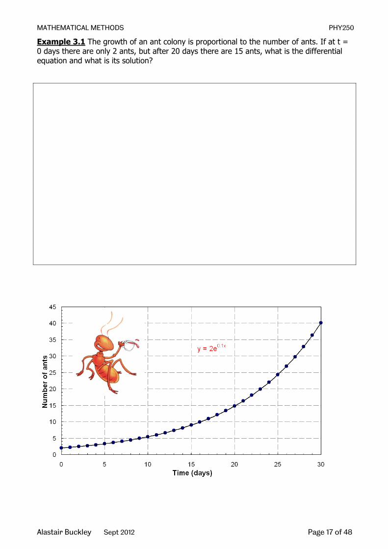
Example 3.1 The growth of an ant colony is proportional to the number of ants. If at t = 0 days there are only 2 ants, but after 20 days there are 15 ants, what is the differential equation and what is its solution?
MATHEMATICAL METHODS PHY250
Alastair Buckley Sept 2012 Page 18 of 48
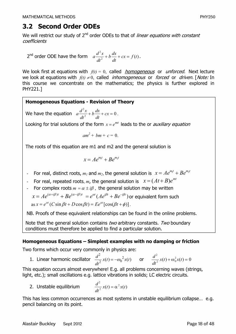
3.2 Second Order ODEs We will restrict our study of 2nd order ODEs to that of linear equations with constant coefficients
2nd order ODE have the form )(2
2
tfcxdtdxb
dtxda =++ .
We look first at equations with f(t) = 0, called homogeneous or unforced. Next lecture we look at equations with f(t) ≠ 0, called inhomogeneous or forced or driven. [Note: In this course we concentrate on the mathematics; the physics is further explored in PHY221.]
Homogeneous Equations – Simplest examples with no damping or friction
Two forms which occur very commonly in physics are:
1. Linear harmonic oscillator 2
202 ( ) ( )d x t x t
dtω= − or 0)()( 2
02
2
=ω+ txtxdtd
This equation occurs almost everywhere! E.g. all problems concerning waves (strings, light, etc.); small oscillations e.g. lattice vibrations in solids; LC electric circuits.
2. Unstable equilibrium )()( 22
2
txtxdtd
α=
This has less common occurrences as most systems in unstable equilibrium collapse… e.g. pencil balancing on its point.
Homogeneous Equations - Revision of Theory
We have the equation 02
2
=++ cxdtdxb
dtxda .
Looking for trial solutions of the form mtx e= leads to the or auxiliary equation
am2 + bm + c = 0. The roots of this equation are m1 and m2 and the general solution is
tmtm BeAex 21 += - For real, distinct roots, m1 and m2, the general solution is tmtm BeAex 21 +=
- For real, repeated roots, m, the general solution is mteBAtx )( += - For complex roots m βα i±= , the general solution may be written
titi BeAex )()( βαβα −+ += )( titit BeAee ββα −+= or equivalent form such as )][cos()cossin( φβββ αα +=+= tEetDtCex tt .
NB. Proofs of these equivalent relationships can be found in the online problems.
Note that the general solution contains two arbitrary constants. Two boundary conditions must therefore be applied to find a particular solution.

MATHEMATICAL METHODS PHY250
Alastair Buckley Sept 2012 Page 19 of 48
Example 3.2 The Linear Harmonic Oscillator
Find the solution of 0)()( 202
2
=ω+ txtxdtd
?
Applying Boundary Conditions
If the particle starts at the origin with velocity V, i.e. x(0) = 0 and 0( ) |t
dx t Vdt = = .

MATHEMATICAL METHODS PHY250
Alastair Buckley Sept 2012 Page 20 of 48
Example 3.3 Unstable Equilibrium
Find the solution of )()( 22
2
txtxdtd
α= ?
Applying Boundary Conditions
Suppose x(0) = L and 0|)(0 ==tdt
tdx. Apply the boundary conditions?
Compare the solutions of equations (1) and (2). They have very different physical characteristics!
Solutions of (1) oscillate for ever.
Solutions of (2) grow to infinity as t increases.

MATHEMATICAL METHODS PHY250
Alastair Buckley Sept 2012 Page 21 of 48
3.3 Homogenous 2nd Order ODE’s
INTRO: Hopefully these equations from PHY102 Waves & Quanta are familiar to you….
Free Oscillation with damping: Forced Oscillation with damping:
02
2
=++ kxdtdxb
dtxdm tHkx
dtdxb
dtxdm Dωcos02
2
=++
In this lecture we consider one more common homogeneous equation then two inhomogeneous equations.
Example 3.4 The Damped Harmonic Oscillator 02 202
2
=++ xdtdx
dtxd ωγ
Looking for solutions of the form emt we obtain the characteristic equation 02 2
02 =++ ωγmm .
This quadratic has two solutions: 20
2 ωγγ −±−=m
Be careful ! There are three different cases. (case i) 2
02 ωγ > (over-damping)
We have two real values for m: 20
21 ωγγ −+−=m and 2
02
2 ωγγ −−−=m .
And the general solution is x(t) = tmtm BeAe 21 + . Both m1 and m2 are negative so x(t) is the sum of two exponential decay terms and so tends pretty quickly, to zero. The effect of the spring has been made of secondary importance to the huge damping, e.g. fire doors.
(case ii) 20
2 ωγ = (critical damping) The characteristic equation has a double root m = -γ , so the general solution is x(t) = e-ωt [A + Bt] as shown earlier. Here the damping has been reduced a little so the spring can act to change the displacement quicker. However the damping is still high enough that the displacement does not pass through the equilibrium position, e.g. car suspension – push down on the wheel arch and hope not to see SHM!
(case iii) 20
2 ωγ < (under-damping)
The roots are complex. Define 220
2 γω −=Ω so Ω±=− 220 γω and Ω±=− i2
02 ωγ .
Then the two allowed values of m can be written Ω+−= im γ1 and Ω−−= im γ2 . The general solution can be written x(t) = e-γt [AeiΩt + Be-iΩt] or x(t) = e-γt [CcosΩt+ DsinΩt] or x(t) = Fe-γt cos(Ωt+φ). See the online Problems Lect3 Prob6. The solution is the product of a sinusoidal term and an exponential decay term – so represents sinusoidal oscillations of decreasing amplitude. E.g. bed springs.

MATHEMATICAL METHODS PHY250
Alastair Buckley Sept 2012 Page 22 of 48
The amplitude will fall to 1/e of its original value after a time γ
τ 1= .
In many physically interesting cases 20
2 ωγ << . In this case Ω ∼ ω0 , so x(t) ≈ Fe-γt cos(ω0t +φ).
In that time τ the oscillator will have made n oscillations. n = f τ and π
ω2
0=f henceπγ
ω2
0=n .
The ratio ω0 / 2γ is called Q, the quality factor. Q is widely used in all areas of physics, a higher Q indicating a lower rate of energy dissipation relative to the oscillation frequency, so oscillations die more slowly. (see PHY102 topic 1 and PHY221).
MATHEMATICAL METHODS PHY250
Alastair Buckley Sept 2012 Page 23 of 48
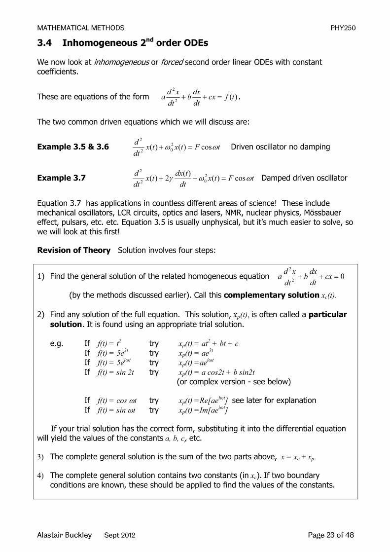
3.4 Inhomogeneous 2nd order ODEs We now look at inhomogeneous or forced second order linear ODEs with constant coefficients.
These are equations of the form )(2
2
tfcxdtdxb
dtxda =++ .
The two common driven equations which we will discuss are:
Example 3.5 & 3.6 tFtxtxdtd ωω cos)()( 2
02
2
=+ Driven oscillator no damping
Example 3.7 tFtxdt
tdxtxdtd ωωγ cos)()(2)( 2
02
2
=++ Damped driven oscillator
Equation 3.7 has applications in countless different areas of science! These include mechanical oscillators, LCR circuits, optics and lasers, NMR, nuclear physics, Mössbauer effect, pulsars, etc. etc. Equation 3.5 is usually unphysical, but it’s much easier to solve, so we will look at this first! Revision of Theory Solution involves four steps:
1) Find the general solution of the related homogeneous equation 02
2
=++ cxdtdxb
dtxda
(by the methods discussed earlier). Call this complementary solution xc(t). 2) Find any solution of the full equation. This solution, xp(t), is often called a particular
solution. It is found using an appropriate trial solution.
e.g. If f(t) = t2 try xp(t) = at2 + bt + c If f(t) = 5e3t try xp(t) = ae3t If f(t) = 5eiωt try xp(t) =aeiωt If f(t) = sin 2t try xp(t) = a cos2t + b sin2t (or complex version - see below) If f(t) = cos ωt try xp(t) =Re[aeiωt] see later for explanation If f(t) = sin ωt try xp(t) =Im[aeiωt] If your trial solution has the correct form, substituting it into the differential equation will yield the values of the constants a, b, c, etc. 3) The complete general solution is the sum of the two parts above, x = xc + xp. 4) The complete general solution contains two constants (in xc). If two boundary
conditions are known, these should be applied to find the values of the constants.

MATHEMATICAL METHODS PHY250
Alastair Buckley Sept 2012 Page 24 of 48
Example 3.5 The Undamped, Driven Oscillator tFtxtxdtd
ω=ω+ cos)()( 202
2
Step 1 The corresponding homogeneous equation is simply the LHO equation. From the last lecture, therefore, we can take, say,
tBtAtxc 00 sincos)( ωω += .
Step 2 We need to find the ‘particular integral’ using a trial solution. We should try
xp(t) = a cos ωt + b sin ωt. Substitute this trial solution into the original equation:
(ω02 − ω2)acosωt + (ω0
2 − ω2)bsinωt = Fcosωt.
Comparing terms we can say that b = 0 and (ω02 − ω2)a = F
Hence the trial solution is a solution provided
220 ωω −
=Fa , i.e. tFtxp ω
ωωcos)( 22
0 −= .
Step 3 So the complete general solution is
tFtBtAtx ωωω
ωω cossincos)( 220
00 −++=
Step 4 Suppose a particle subject to the equation above is known to be at rest at x = L at t = 0.
This means we have the boundary conditions x(0) = L and 0| 0 ==tdtdx .
Substitute t = 0 in the general solution given above:
LFAx =−
++= 220
0)0(ωω
Differentiating the general solution, then substituting t = 0 gives 0 0Bω =
Hence B = 0 and 220 ωω −
−=FLA so the solution is:
tFtFLtx ωωω
ωωω
coscos)()( 220
0220 −
+−
−=
This can be written as )cos(cos)(
cos)( 0220
0 ttFtLtx ωωωω
ω −−
+= .

MATHEMATICAL METHODS PHY250
Alastair Buckley Sept 2012 Page 25 of 48
A few comments
1. Note that the solution is clearly not valid for 0ω=ω !
2. The ratio Ftx )(
is sometimes called the response of the oscillator. It is a function of
ω. It is positive for ω < ω0, negative for ω > ω0 . This means that at low frequency the oscillator follows the driving force but at high frequencies it is always going in the ‘wrong’ direction.
Example 3.6 Solution using Complex Numbers The particular integral of the equation above was easy to find because a trial function of the form xp(t) = a cos ωt + b sin ωt worked. In our next equation (a driven oscillator with damping) this trial function would also work ... but the algebra gets very messy. It is easier to use complex numbers. To learn the complex method we will use it to solve equation 4 again for the particular integral.
Compare the original equation tFtxtxdtd
ω=ω+ cos)()( 202
2
(A)
With the equation tiFetXtXdtd ωω =+ )()( 2
02
2
(B)
We know Fcosω t = Re(Feiωt), so if equation (B) has (complex) solutions X(t) then the solutions of equation (A) will be the real part of these: x(t) = Re(X(t)). If the function on the RHS of (A) was sinωt then we could use the same approach but at the end take the imaginary part.
i.e. first we solve tiFetXtXdtd ωω =+ )()( 2
02
2
.
This is easy: we take a trial solution of the form X = Aeiωt.
Substituting this in gives: tititi FeeAAedtd ωωω ωωωω =+−=+ )()()( 2
022
02
2
MATHEMATICAL METHODS PHY250
Alastair Buckley Sept 2012 Page 26 of 48
Hence )(
)( 220 ωω
ω−
=FA so tieFtX ω
ωω )()( 22
0 −=
To find the particular solution we take the real part: x(t) = Re(X(t)) = )(
cos22
0 ωωω
−tF
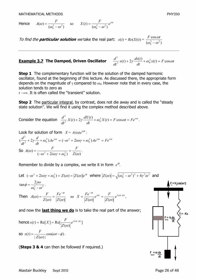
Example 3.7 The Damped, Driven Oscillator tFtxdt
tdxtxdtd ωωγ cos)()(2)( 2
02
2
=++
Step 1 The complementary function will be the solution of the damped harmonic oscillator, found at the beginning of this lecture. As discussed there, the appropriate form depends on the magnitude of γ compared to ω0. However note that in every case, the solution tends to zero as t →∞. It is often called the “transient” solution. Step 2 The particular integral, by contrast, does not die away and is called the “steady state solution”. We will find it using the complex method described above.
Consider the equation tiFetFtXdt
tdXtXdtd ωωωγ ==++ cos)()(2)( 2
02
2
.
Look for solution of form X = A(ω)eiωt :
tititi FeAeiAedtd
dtd ωωω ωωγωωγ =++−=++ )2()2( 2
022
02
2
So )()2(
)( 20
2 ωωωγωω
ZF
iFA =
++−= .
Remember to divide by a complex, we write it in form eiφ. Let φωωωωγω ieZZi )()()2( 2
02 ==++− where 22222
0 4)()( ωγωωω +−=Z and
220
2tanωω
γωφ−
= .
Then )()(
)(ωω
ωφ
ZFe
ZFA
i−
== so )(
)()(φωω
φ
ωω−
−
== titii
eZ
FeZFeX ,
and now the last thing we do is to take the real part of the answer;
hence ])(
Re[]Re[)( )( φω
ω−== tie
ZFXtx
so ( ) cos( )| ( ) |
Fx t tZ
ω φω
= − .
(Steps 3 & 4 can then be followed if required.)

MATHEMATICAL METHODS PHY250
Alastair Buckley Sept 2012 Page 27 of 48
In cases where the damping is small, the amplitude has a strong peak at 0ω ω≈ and the quality factor Q is again an important indicator. Closing remarks We have focussed on the mathematics of solving generic harmonic oscillator equations. By replacing ω, γ, etc. with appropriate constants, you should now be able to solve equations for all mechanical oscillators, oscillations in electrical LCR circuits, and numerous other oscillators! PHY221 and other courses will explore more of the physical significance of the solutions found here. References The material of lectures 3&4 is covered very thoroughly, with many real physical examples, by French:
Undamped, undriven LHO 7-9 Damped*, undriven LHO & Q-factor 10-16 Undamped, driven LHO: steady state 20-24 … again using complex exponentials 24-25 Damped*, driven LHO: steady state 25-28
Further discussion of Q, transients, resonance, etc. 31-42 Electrical, optical & nuclear examples 42-52 [*Note that French uses a damping constant γ while we have used 2γ]

MATHEMATICAL METHODS PHY250
Alastair Buckley Sept 2012 Page 28 of 48
Online problems (Topic 3, questions 1-11)
1. Verify the solution stated in the notes for )()( 22
2
txdt
txd α= subject to Lx =)0( and
0)(
0
==tdt
tdx
2. Given that )()( 22
2
txdt
txd α= and at 0,0 == xt and 0=
=tdt
dxv find solution and then
plot x against αt.
3. Solve 0442
2
=+− ydxdy
dxyd
with boundary conditions of 4)0( =y and 0)0(=
dxdy
4. Solve 0432
2
=−+ xdtdx
dtxd
5. Solve 0222
2
=++ ydxdy
dxyd
6. Re-write your answer to 3 in terms of cos and sin, removing all complex formatting
7. Solve 01782
2
=+− ydtdy
dtyd
with boundary conditions 4)0( −=y and 1)0(' −=y
8. Atmospheric physics – a change in height h∆ causes the pressure to drop by P∆ .
This follows the equation hgP ∆−=∆ ρ where ρ is the density of air. However the density is also a functions of the pressure P, so as the height increases the drop in
pressure is not linear (as it would have been if p was constant). kTmP
=ρ where m
is the mass of one molecule, k is the Boltzmann constant and T is temperature and P is pressure. Write down the 1st order differential equation that defines the change in pressure with height and solve it.
9. The equation describing the process of discharging a capacitor which is initially
charged to Vb is 0=+CQ
dtdQR where bCVQ = at 0=t
10. Solve )3cos(222
2
xydxdy
dxyd
=++
11. Solve )2sin(3592 2
2
xydxdy
dxyd
=−−

MATHEMATICAL METHODS PHY250
Alastair Buckley Sept 2012 Page 29 of 48
Topic 4. Fourier Series References Jordan & Smith Ch.26, Boas Ch.7, Kreyszig Ch.11 Some fun ‘java applet’ demonstrations are available on the web. Try putting ‘Fourier series applet’ into Google and looking at the sites from jhu, Falstad and Maths Online Gallery. 4.1 Introduction to Fourier Series Consider a length of string fixed between rigid supports. The full behaviour of this system can be found by solving a wave equation – a partial differential equation. We will do this later in the course. For now we will just recall the basic properties of waves of strings which we already know: There is a fundamental mode of vibration. Call the frequency of this mode f and the time period T. Then there are various harmonics. These have frequency 2f, 3f, 4f, 5f, …, nf, … In practice, when a piano or guitar or other string is hit or plucked, it does not vibrate purely in one mode – the displacement of the string is not purely sinusoidal, the sound emitted is not all of one frequency. In practice, one normally hears a large amount of the fundamental plus smaller amounts of various harmonics. The proportions in which the different frequencies are present varies – hence a guitar sounds different from a violin or a piano, and a violin sounds different if it is bowed from if it is plucked! (See http://www.jhu.edu/~signals/listen/music1.html pages 1&2) Remember that if the fundamental frequency has frequency f, its period T = 1/f. A harmonic wave of frequency nf will then have a period T/n, but obviously also repeats with period T. So if we add together sinusoidal waves of frequency f, 2f, 3f, 4f,… the result is a (non-sinusoidal) waveform which is periodic with the same period T as the fundamental frequency, f = 1/T. [E.g. play with http://www.falstad.com/fourier/ ] Sometimes we use the angular frequency ω where the nth harmonic has ωn = 2πnf = 2πn/Τ. The various harmonics are then of the form Asinωnt.
sinωt
0.5 sin2ωt
0.5 sin3ωt
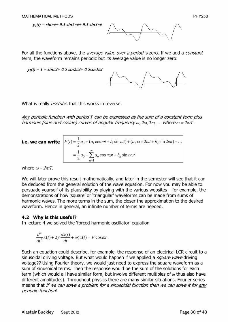
MATHEMATICAL METHODS PHY250
Alastair Buckley Sept 2012 Page 30 of 48
y1(t) = sinωt+ 0.5 sin2ωt+ 0.5 sin3ωt
For all the functions above, the average value over a period is zero. If we add a constant term, the waveform remains periodic but its average value is no longer zero:
y2(t) = 1 + sinωt+ 0.5 sin2ωt+ 0.5sin3ωt
What is really useful is that this works in reverse:
Any periodic function with period T can be expressed as the sum of a constant term plus harmonic (sine and cosine) curves of angular frequency ω, 2ω, 3ω, ... where ω = 2π/T .
i.e. we can write
0 1 1 2 2
01
1( ) ( cos sin ) ( cos 2 sin 2 )21 cos sin2 n n
n
F t a a t b t a t b t
a a n t b n t
ω ω ω ω
ω ω∞
=
= + + + + +
= + +∑
K
where ω = 2π/T. We will later prove this result mathematically, and later in the semester will see that it can be deduced from the general solution of the wave equation. For now you may be able to persuade yourself of its plausibility by playing with the various websites – for example, the demonstrations of how ‘square’ or ‘triangular’ waveforms can be made from sums of harmonic waves. The more terms in the sum, the closer the approximation to the desired waveform. Hence in general, an infinite number of terms are needed. 4.2 Why is this useful? In lecture 4 we solved the ‘forced harmonic oscillator’ equation
tFtxdt
tdxtxdtd ωωγ cos)()(2)( 2
02
2
=++ .
Such an equation could describe, for example, the response of an electrical LCR circuit to a sinusoidal driving voltage. But what would happen if we applied a square wave driving voltage?? Using Fourier theory, we would just need to express the square waveform as a sum of sinusoidal terms. Then the response would be the sum of the solutions for each term (which would all have similar form, but involve different multiples of ω thus also have different amplitudes). Throughout physics there are many similar situations. Fourier series means that if we can solve a problem for a sinusoidal function then we can solve it for any periodic function!
MATHEMATICAL METHODS PHY250
Alastair Buckley Sept 2012 Page 31 of 48
And periodic functions appear everywhere! Examples of periodicity in time: a pulsar, a train of electrical pulses, the temperature variation over 24 hours or the average daily temperature over a year (approximately). Examples of periodicity in space: a crystal lattice, an array of magnetic domains, etc.
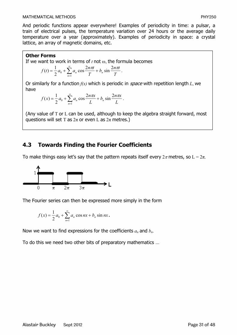
4.3 Towards Finding the Fourier Coefficients To make things easy let’s say that the pattern repeats itself every 2π metres, so L = 2π.
The Fourier series can then be expressed more simply in the form
∑∞
=
++=1
0 sincos21)(
nnn nxbnxaaxf .
Now we want to find expressions for the coefficients an and bn. To do this we need two other bits of preparatory mathematics …
Other Forms If we want to work in terms of t not ω, the formula becomes
∑∞
=
++=1
02sin2cos
21)(
nnn T
tnbT
tnaatf ππ .
Or similarly for a function f(x) which is periodic in space with repetition length L, we have
∑∞
=
++=1
02sin2cos
21)(
nnn L
xnbL
xnaaxf ππ .
(Any value of T or L can be used, although to keep the algebra straight forward, most questions will set T as 2π or even L as 2π metres.)

MATHEMATICAL METHODS PHY250
Alastair Buckley Sept 2012 Page 32 of 48
4.4 Average Value of a Function Consider a function y = f(x). The average value of the function between x = a and x = b is defined to be
∫−b
adxxf
ab)(1 .
Geometrically this means that the area under the curve f(x) between a and b is equal to the area of a rectangle of width (b-a) and height equal to this average value. Note that while average values can be found by evaluating the above integral, sometimes they can be identified more quickly from symmetry considerations, a sketch graph and common sense! Two particularly important results are:
Actually both these results can be generalized. It is easily shown that:
0cos21sin
21 2
0
2
0== ∫∫
ππ
ππdxnxdxnx and
21cos
21sin
21 2
0
22
0
2 == ∫∫ππ
ππdxnxdxnx for n ≠ 0
Hence 0cossin2
0
2
0== ∫∫
ππdxnxdxnx and π
ππ== ∫∫
2
0
22
0
2 cossin dxnxdxnx (n ≠ 0)
Note: We have written all the integrals over [0, 2π] but any interval of width 2π can be used, e.g. [–π, π], [13.1π, 15.1π], etc. 4.5 Orthogonality (Proofs in the Appendix) Sines and cosines have an important property called ‘orthogonality’: The product of two different sine or cosine functions, integrated over a period, gives zero:
0cossin2
0=∫
πdxmxnx for all n, m
0coscossinsin2
0
2
0== ∫∫
ππdxmxnxdxmxnx
for all n ≠ m Again we can integrate over any period. Equipped with these results we can now find the Fourier coefficients …
The average value of a sine or cosine function over a period is zero:
0cos21sin
21sin
21 2
0
2
0=== ∫∫∫−
πππ
π πππdxnxdxnxdxnx .
The average value of cos2 or sin2 over a period is ½:
2 22 20 0
1 1 1sin cos2 2 2
x dx x dxπ π
π π= =∫ ∫ .

MATHEMATICAL METHODS PHY250
Alastair Buckley Sept 2012 Page 33 of 48
4.6 Fourier Coefficients – Derivation
Earlier we said any function f(x) with period 2π can be written
∑∞
=
++=1
0 sincos21)(
nnn nxbnxaaxf .
Take this equation and integrate both sides over a period (any period):
∑ ∫∫∫∫∞
=
++=
1
2
0
2
0
2
00
2
0sincos
21)(
nnn dxnxbdxnxadxadxxf
ππππ
Clearly on the RHS the only non-zero term is the a0 term:
00
2
00
2
0)02(
21
21)( aadxadxxf ππ
ππ=−== ∫∫
hence ∫=π
π2
00 )(1 dxxfa i.e. a0 /2 is the average value of the function f(x).
Now take the original equation again, multiply both sides by cosx, then integrate over a period:
∑ ∫∫∫∫∞
=
++=
1
2
0
2
0
2
00
2
0cossincoscoscos
21cos)(
nnn dxxnxbdxxnxaxdxaxdxxf
ππππ
On the RHS, this time only the a1 term survives as it is the only term where n=1 (see Orthogonality.)
ππππ
1
2
0
21
2
01
2
0coscoscoscos)( adxxadxxxaxdxxf === ∫∫∫
hence ∫=π
π2
01 cos)(1 xdxxfa .
The method for finding the coefficients an should thus be clear. To find a general expression for an we can take the equation, multiply both sides by cosmx, then integrate over a period:
∑ ∫∫∫∫∞
=
++=
1
2
0
2
0
2
00
2
0cossincoscoscos
21cos)(
nnn dxmxnxbdxmxnxamxdxamxdxxf
ππππ
On the RHS, only the am term survives the integration:
πππ
mm adxmxamxdxxf == ∫∫2
0
22
0coscos)( hence ∫=
π
π2
0cos)(1 mxdxxfam .
In a similar way, multiplying both sides by sinmx, then integrating over a period we get:
∫=π
π2
0sin)(1 dxmxxfbm

MATHEMATICAL METHODS PHY250
Alastair Buckley Sept 2012 Page 34 of 48
4.7 Summary of Results
A function f(x) with period 2π can be expressed as
∑∞
=
++=1
0 sincos21)(
nnn nxbnxaaxf
where ∫=π
π2
00 )(1 dxxfa , ∫=π
π2
0cos)(1 dxnxxfan , ∫=
π
π2
0sin)(1 dxnxxfbn .
The more general expression from page 2 can be written as:- A function f(x) with period L can be expressed as
∑∞
=
++=1
02sin2cos
21)(
nnn L
xnbL
xnaaxf ππ
where ∫=L
dxxfL
a00 )(2 , ∫=
L
n dxL
xnxfL
a0
2cos)(2 π , ∫=L
n dxL
xnxfL
b0
2sin)(2 π .
Note
1) The formula for a0 can be obtained from the formula for an just by setting n = 0. 2) The integrals above are written over [0, 2π] and [0, L] but any convenient interval of width one period may be used, and this will be dependent on the nature of the function (see examples and the online Problems). 3) The equations can be easily adapted to work with other variables or periodicities. For example, for a function periodic in time with period T just replace x by t and L by T. 4) A few books use the alternative form
00
1
( ) cos( )2 n n
n
dF t d n tω θ∞
=
= + +∑ and find values of dn and θn.

MATHEMATICAL METHODS PHY250
Alastair Buckley Sept 2012 Page 35 of 48
4.8 Examples
Example 4.1 Find a Fourier series for the square wave shown.
We have
<<<<
=ππ
π20
01)(
xx
xf The period is 2π.
Think: After reaching your answer, ask yourself: is this result sensible?
- Does the term a0/2 look like an appropriate value for the average value of the function over a period?
- Would we expect this function to be made mainly of sines or of cosines? (See later for symmetry).
- In what proportions would we expect to find the fundamental and the various harmonics?
(You can also try checking your answer by ‘building’ the series at http://www.falstad.com/fourier/ or http://www.univie.ac.at/future.media/moe/galerie/fourier/fourier.html )
0 π 2π 3π x
1

MATHEMATICAL METHODS PHY250
Alastair Buckley Sept 2012 Page 36 of 48
Example 4.2 Find a Fourier series of the function shown:
Again the period is 2π. But this time it is easiest to work with the range [-π, π]. If we wanted we could use the range [0,2π] and get the same answer, but it would be fiddlier. Between -π and π, f(x) is a straight line with gradient 1 and a Y-intercept of π. So we can write f(x) = x + π −π < x < π. Lets find a0
( ) πππ
πππππ
ππ
πππ
π
π
π
π
π
π221
221
21)(1)(1 22
22
22
0 ==
−−
+=
+=+==
−−− ∫∫ xxdxxdxxfa
Lets find an
== ∫−
π
ππdxnxxfan cos)(1
∫∫∫ −−−+=+
π
π
π
π
π
ππ
πππ
πdxnxdxnxxdxnxx cos1cos1cos)(1
We must integrate ∫−
π
πdxnxx cos by parts:
∫ ∫−= vduuvudv
u = x dv = cos nx dx du = dx
nxn
nxdxv sin1cos == ∫
So 0cos1sinsin1sincos 2 =
+=−=
−−− ∫∫
π
π
π
π
π
πnx
nnx
nxnxdx
nnx
nxdxnxx
(see p.3 average value)
Going back to an ,
== ∫−
π
ππdxnxxfan cos)(1 0cos10cos)(1
=+=+ ∫∫ −−
π
π
π
ππ
ππ
πdxnxdxnxx
(see p.3 average value)
MATHEMATICAL METHODS PHY250
Alastair Buckley Sept 2012 Page 37 of 48
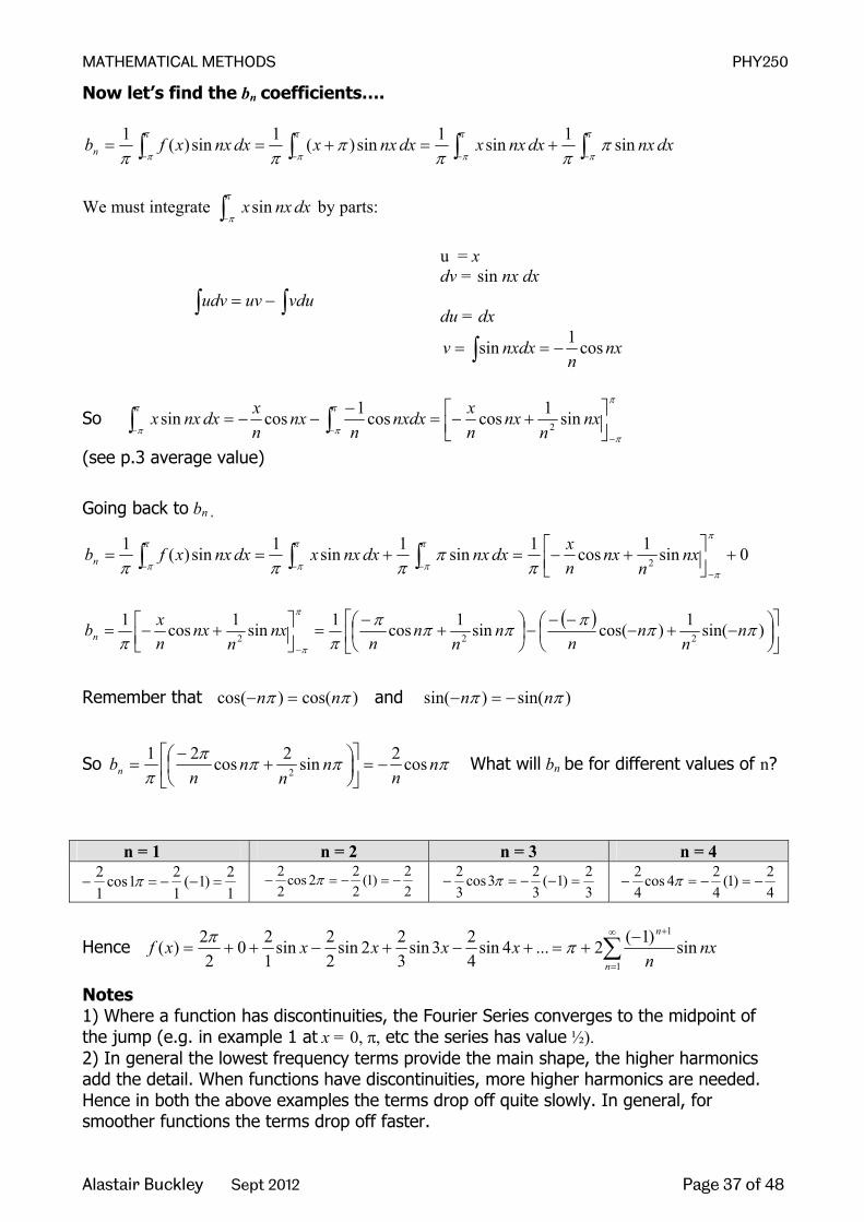
Now let’s find the bn coefficients….
∫∫∫∫ −−−−+=+==
π
π
π
π
π
π
π
ππ
πππ
ππdxnxdxnxxdxnxxdxnxxfbn sin1sin1sin)(1sin)(1
We must integrate ∫−
π
πdxnxxsin by parts:
∫ ∫−= vduuvudv
u = x dv = sin nx dx du = dx
nxn
nxdxv cos1sin −== ∫
So π
π
π
π
π
π−
−− ∫∫
+−=
−−−= nx
nnx
nxnxdx
nnx
nxdxnxx sin1coscos1cossin 2
(see p.3 average value)
Going back to bn ,
0sin1cos1sin1sin1sin)(12 +
+−=+==
−−−− ∫∫∫
π
π
π
π
π
π
π
π ππ
πππnx
nnx
nxdxnxdxnxxdxnxxfbn
( )
−+−
−−−
+
−=
+−=
−
)sin(1)cos(sin1cos1sin1cos1222 ππππππ
ππ
π
π
nn
nn
nn
nn
nxn
nxnxbn
Remember that )cos()cos( ππ nn =− and )sin()sin( ππ nn −=−
So πππππ
nn
nn
nn
bn cos2sin2cos212 −=
+
−= What will bn be for different values of n?
n = 1 n = 2 n = 3 n = 4
12)1(
121cos
12
=−−=− π 22)1(
222cos
22
−=−=− π 32)1(
323cos
32
=−−=− π 42)1(
424cos
42
−=−=− π
Hence ∑∞
=
+−+=+−+−++=
1
1
sin)1(2...4sin423sin
322sin
22sin
120
22)(
n
n
nxn
xxxxxf ππ
Notes 1) Where a function has discontinuities, the Fourier Series converges to the midpoint of the jump (e.g. in example 1 at x = 0, π, etc the series has value ½). 2) In general the lowest frequency terms provide the main shape, the higher harmonics add the detail. When functions have discontinuities, more higher harmonics are needed. Hence in both the above examples the terms drop off quite slowly. In general, for smoother functions the terms drop off faster.
MATHEMATICAL METHODS PHY250
Alastair Buckley Sept 2012 Page 38 of 48
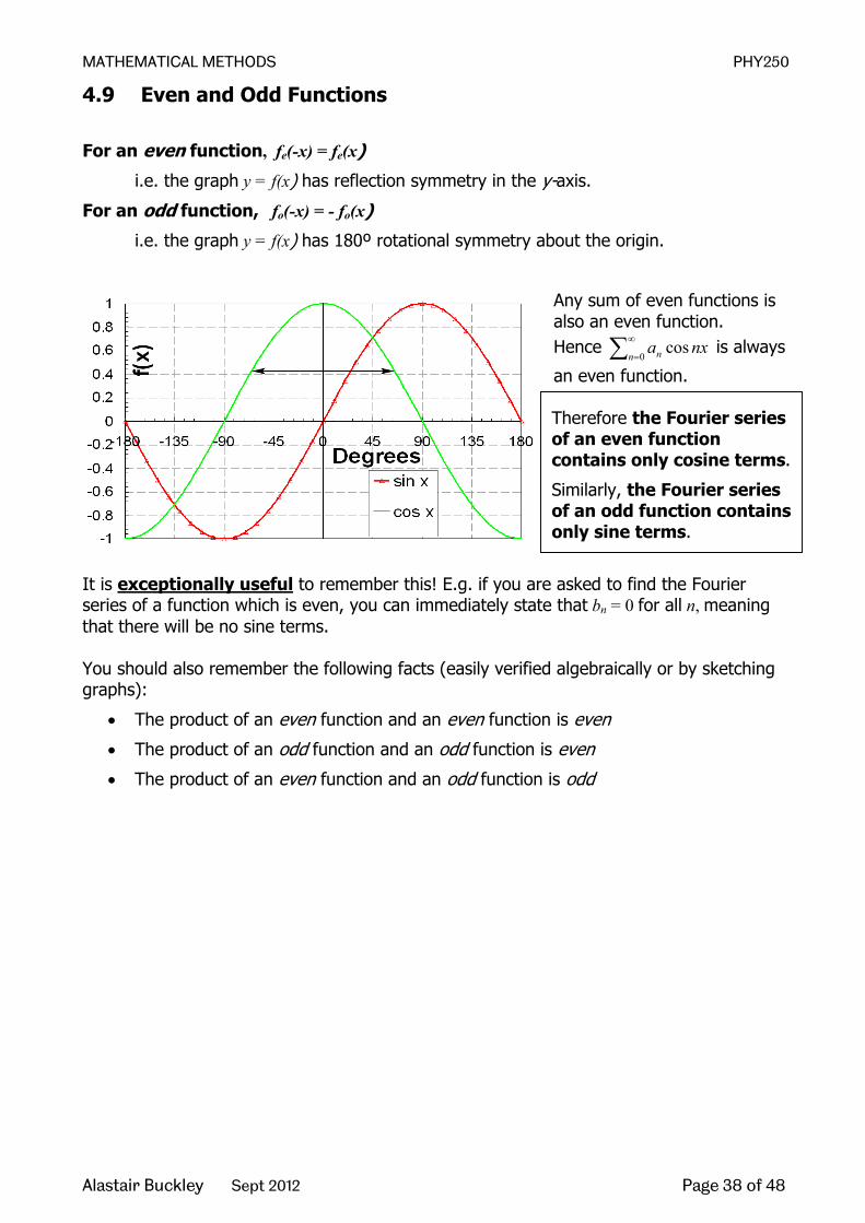
Therefore the Fourier series of an even function contains only cosine terms.
Similarly, the Fourier series of an odd function contains only sine terms.
4.9 Even and Odd Functions
For an even function, fe(-x) = fe(x)
i.e. the graph y = f(x) has reflection symmetry in the y-axis.
For an odd function, fo(-x) = - fo(x)
i.e. the graph y = f(x) has 180º rotational symmetry about the origin.
Any sum of even functions is also an even function. Hence ∑∞
=0cos
n n nxa is always
an even function.
It is exceptionally useful to remember this! E.g. if you are asked to find the Fourier series of a function which is even, you can immediately state that bn = 0 for all n, meaning that there will be no sine terms. You should also remember the following facts (easily verified algebraically or by sketching graphs):
• The product of an even function and an even function is even
• The product of an odd function and an odd function is even
• The product of an even function and an odd function is odd

MATHEMATICAL METHODS PHY250
Alastair Buckley Sept 2012 Page 39 of 48
Example 4.3 Find a Fourier series of the function shown:
The period is L. As discussed earlier we can integrate over any full period e.g. ∫
L
0or ∫−
2/
2/
L
L
The function is even and can be written f(x) =1 for 4
34
LxL ≤≤ . Therefore there will be no
sine terms (bn = 0 for all n) and I feel like integrating between 0 and L. The series will have form
∑∞
=
+=1
02cos
21)(
nn L
xnaaxf π where ∫=L
dxxfL
a00 )(2 and ∫=
L
n dxL
xnxfL
a0
2cos)(2 π .
So ][ 1212)(2 4/34/
4/3
4/00 ==== ∫∫ LL
L
L
Lx
Ldx
Ldxxf
La
−=
=== ∫∫ )
42(sin)
46(sin12sin
222cos122cos)(2 4/3
4/
4/3
4/0
πππ
ππ
ππ nnnL
xnLn
LdxL
xnL
dxL
xnxfL
aL
L
L
L
L
n
−=
−= )
2(sin)
23(sin1)
42(sin)
46(sin1 ππ
πππ
πnn
nnn
nan
Expression for an is not very pretty and easy to make mistakes with. Write out a table to help with assignment of coefficients….
n = 1 n = 2 n = 3 n = 4
πππ
π2)
2(sin)
23(sin1
−=
−
0)
22(sin)
26(sin
21
=
−
πππ
πππ
π 32)
23(sin)
29(sin
31
=
−
0)
24(sin)
212(sin
41
=
−
πππ
n = 5 n = 6 n = 7 n = 8
πππ
π 52)
25(sin)
215(sin
51
−=
−
0)
26(sin)
218(sin
61
=
−
πππ
πππ
π 72)
27(sin)
221(sin
71
=
−
0)
28(sin)
224(sin
81
=
−
πππ
So ...10cos526cos
322cos2
21)( +
−
+
−=
Lx
Lx
Lxxf π
ππ
ππ
π
MATHEMATICAL METHODS PHY250
Alastair Buckley Sept 2012 Page 40 of 48
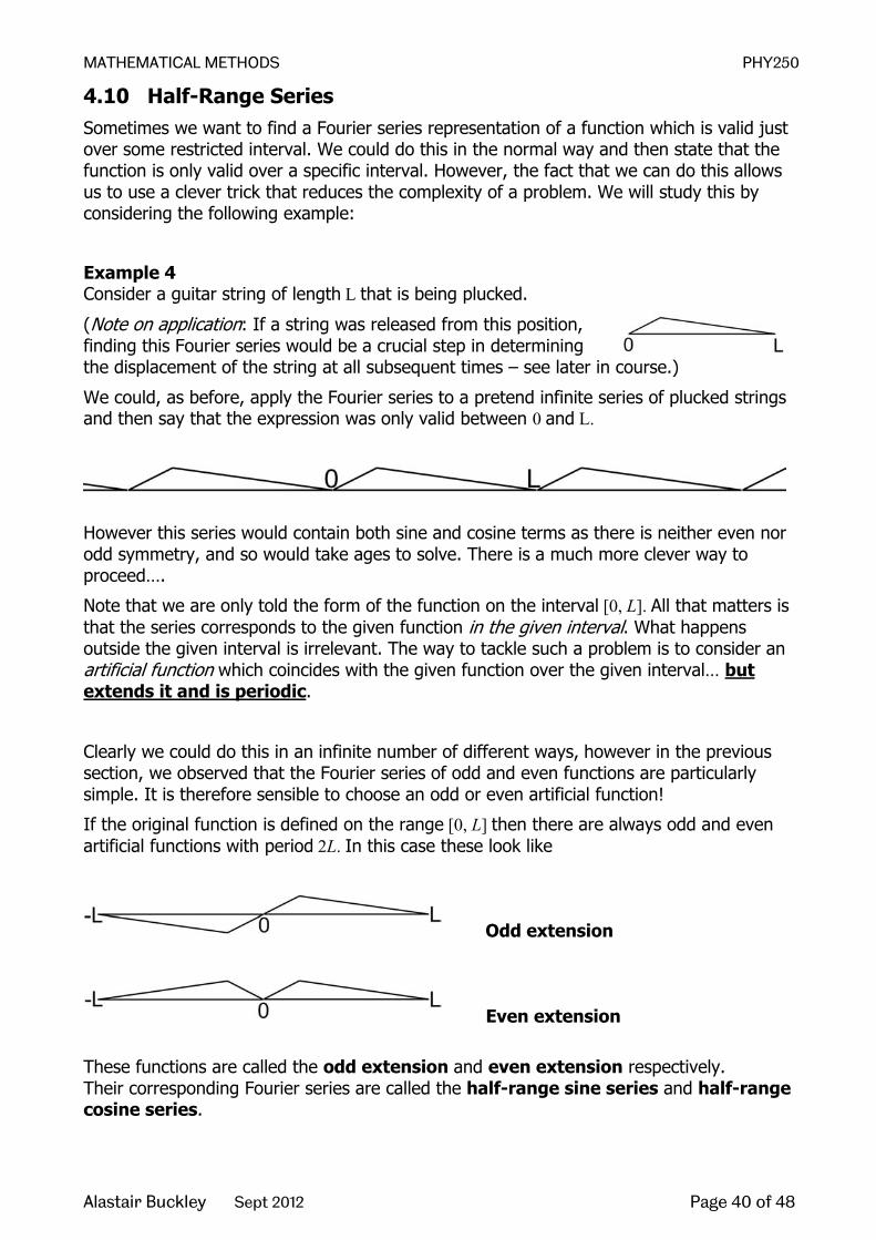
4.10 Half-Range Series Sometimes we want to find a Fourier series representation of a function which is valid just over some restricted interval. We could do this in the normal way and then state that the function is only valid over a specific interval. However, the fact that we can do this allows us to use a clever trick that reduces the complexity of a problem. We will study this by considering the following example:
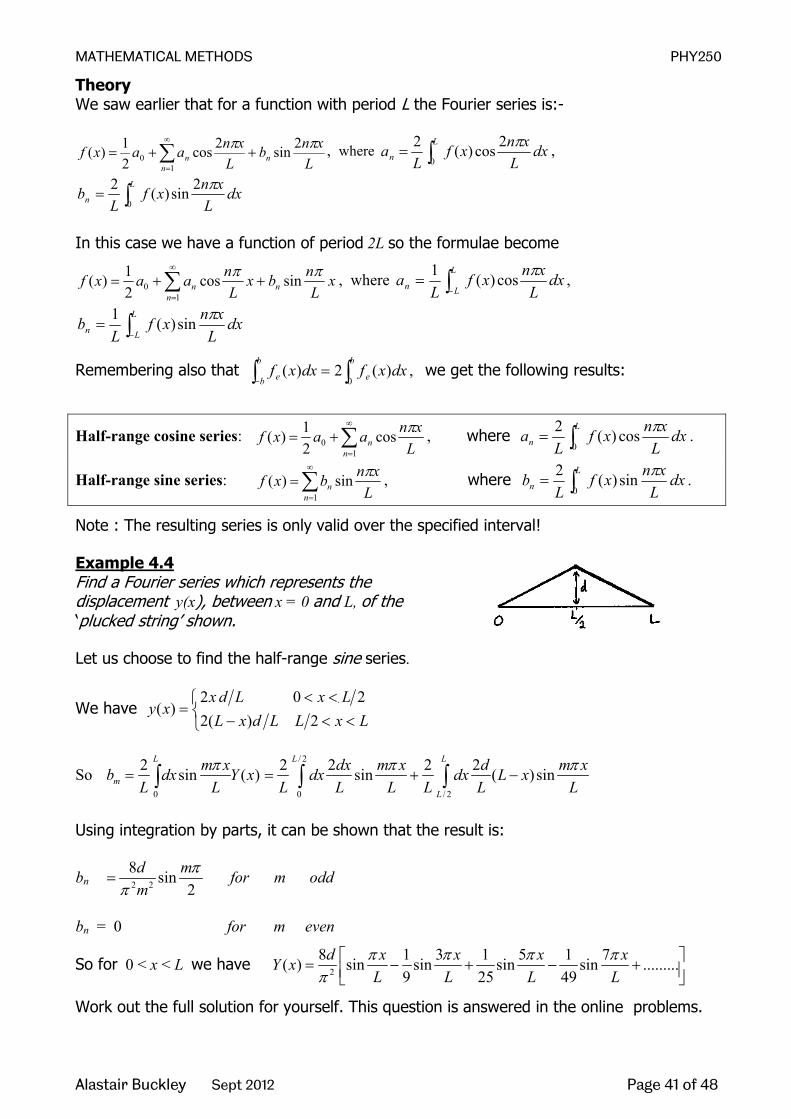
Example 4 Consider a guitar string of length L that is being plucked.
(Note on application: If a string was released from this position, finding this Fourier series would be a crucial step in determining the displacement of the string at all subsequent times – see later in course.)
We could, as before, apply the Fourier series to a pretend infinite series of plucked strings and then say that the expression was only valid between 0 and L.
However this series would contain both sine and cosine terms as there is neither even nor odd symmetry, and so would take ages to solve. There is a much more clever way to proceed….
Note that we are only told the form of the function on the interval [0, L]. All that matters is that the series corresponds to the given function in the given interval. What happens outside the given interval is irrelevant. The way to tackle such a problem is to consider an artificial function which coincides with the given function over the given interval… but extends it and is periodic.
Clearly we could do this in an infinite number of different ways, however in the previous section, we observed that the Fourier series of odd and even functions are particularly simple. It is therefore sensible to choose an odd or even artificial function!
If the original function is defined on the range [0, L] then there are always odd and even artificial functions with period 2L. In this case these look like
Odd extension
Even extension These functions are called the odd extension and even extension respectively. Their corresponding Fourier series are called the half-range sine series and half-range cosine series.
MATHEMATICAL METHODS PHY250
Alastair Buckley Sept 2012 Page 41 of 48
Theory We saw earlier that for a function with period L the Fourier series is:-
∑∞
=
++=1
02sin2cos
21)(
nnn L
xnbL
xnaaxf ππ , where ∫=L
n dxL
xnxfL
a0
2cos)(2 π ,
∫=L
n dxL
xnxfL
b0
2sin)(2 π
In this case we have a function of period 2L so the formulae become
∑∞
=
++=1
0 sincos21)(
nnn x
Lnbx
Lnaaxf ππ , where ∫−
=L
Ln dxL
xnxfL
a πcos)(1 ,
∫−=
L
Ln dxL
xnxfL
b πsin)(1
Remembering also that ∫∫ =−
b
e
b
b e dxxfdxxf0
)(2)( , we get the following results:
Half-range cosine series: ∑∞
=
+=1
0 cos21)(
nn L
xnaaxf π , where ∫=L
n dxL
xnxfL
a0
cos)(2 π .
Half-range sine series: ∑∞
=
=1
sin)(n
n Lxnbxf π , where ∫=
L
n dxL
xnxfL
b0
sin)(2 π .
Note : The resulting series is only valid over the specified interval! Example 4.4 Find a Fourier series which represents the displacement y(x), between x = 0 and L, of the ‘plucked string’ shown. Let us choose to find the half-range sine series.
We have
<<−<<
=LxLLdxL
LxLdxxy
2)(2202
)(
So 0
2 sin ( )L
mm xb dx Y x
L Lπ
= ∫/ 2
0 / 2
2 2 2 2sin ( )sinL L
L
dx m x d m xdx dx L xL L L L L L
π π= + −∫ ∫
Using integration by parts, it can be shown that the result is:
bn 2 2
8 sin2
d m for m oddm
ππ
=
bn = 0 for m even
So for 0 < x < L we have 2
8 1 3 1 5 1 7( ) sin sin sin sin .........9 25 49
d x x x xY xL L L L
π π π ππ
= − + − +
Work out the full solution for yourself. This question is answered in the online problems.
MATHEMATICAL METHODS PHY250
Alastair Buckley Sept 2012 Page 42 of 48
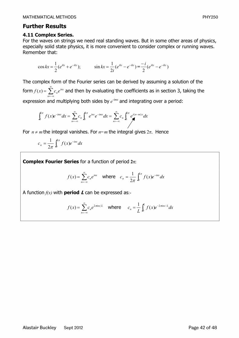
Further Results
4.11 Complex Series. For the waves on strings we need real standing waves. But in some other areas of physics, especially solid state physics, it is more convenient to consider complex or running waves. Remember that:
1 1cos ( ); sin ( )2 2
ikx ikx ikx ikxkx e e kx e ei
− −= + = − = )(2
ikxikx eei −−−
The complex form of the Fourier series can be derived by assuming a solution of the
form ∑∞
−∞=
=n
inxnecxf )( and then by evaluating the coefficients as in section 3, taking the
expression and multiplying both sides by e-imx and integrating over a period:
∑ ∫∑ ∫∫∞
−∞=
−∞
−∞=
−− ==n
xmnin
n
imxinxn
imx dxecdxeecdxexfπππ 2
0
)(2
0
2
0)(
For n m≠ the integral vanishes. For n=m the integral gives 2π. Hence
dxexfc inxn
−∫=π
π2
0)(
21
Complex Fourier Series for a function of period 2π:
∑∞
−∞=
=n
inxnecxf )( where dxexfc inx
n−∫=
π
π2
0)(
21
A function f(x) with period L can be expressed as:-
∑∞
−∞=
=n
Linxnecxf π2)( where dxexf
Lc LinxL
n/2
0)(1 π−∫=

MATHEMATICAL METHODS PHY250
Alastair Buckley Sept 2012 Page 43 of 48
Let’s have a look at an example of complex Fourier series. Example 4.5
Find the complex Fourier series for f(x) = x in the range -2 < x < 2 if the repeat period is 4.

MATHEMATICAL METHODS PHY250
Alastair Buckley Sept 2012 Page 44 of 48
4.12 Parseval’s Theorem Consider again the Fourier series
∑∞
=
++=1
0 sincos21)(
nnn nxbnxaaxf .
Square both sides then integrate over a period:
[ ] dxnxbnxaadxxfn
nn
n
2
110
2
0
2
0
2 sincos21)(
++= ∑∑∫∫
∞
=
∞
=
ππ
The RHS will give both squared terms and cross term. When we integrate, all the cross terms will vanish. All the squares of the cosines and sines integrate to give π (half the period. Hence…
[ ] ][4
2)( 2
1
22
02
0
2n
nn baadxxf ++= ∑∫
∞
=
πππ
The energy in a vibrating string or an electrical signal is proportional to an integral like
[ ] dxxf∫π2
0
2)( .
Hence Parseval’s theorem tells us that the total energy in a vibrating system is equal to the sum of the energies in the individual modes. From PHY101…
MATHEMATICAL METHODS PHY250
Alastair Buckley Sept 2012 Page 45 of 48
4.13 Appendix: Orthogonality At a fundamental mathematical level, the reason the Fourier series works – the reason any periodic function can be expressed as a sum of sine and cosine functions – is that sines and cosines are orthogonal. In general, a set of functions u1(x), u2(x), … , un(x),… is said to be orthogonal on the interval [a, b] if
=≠
=∫ mncmn
dxxuxun
b
a mn
0)()( (where cn is a constant).
Here we will prove that function sinnx, cosmx, etc are orthogonal on the interval [0, 2π].
1. ∫∫ −−+=ππ 2
0
2
0)sin()sin(
21cossin dxxmnxmndxmxnx
[Using sin( ) sin( ) 2sin cosa b a b a b+ − − = ]
0)cos(1)cos(121 2
0
=
−
−++
+−=
π
xmnmn
xmnmn
Hence 0cossin2
0=∫
πdxmxnx for n ≠ m
2. ∫∫ +−−=ππ 2
0
2
0)cos()cos(
21sinsin dxxmnxmndxmxnx
[Using cos( ) cos( ) 2sin sina b a b a b− − + = ]
0)sin(1)sin(121 2
0
=
−
−−−
−=
π
xmnmn
xmnmn
Hence 0sinsin2
0=∫
πdxmxnx for n ≠ m.
3. ∫∫ −++=ππ 2
0
2
0)cos()cos(
21coscos dxxmnxmndxmxnx
[Using cos( ) cos( ) 2cos cosa b a b a b− + + = ]
0)sin(1)sin(121 2
0
=
−
−++
+=
π
xmnmn
xmnmn
Hence 0coscos2
0=∫
πdxmxnx for n ≠ m

MATHEMATICAL METHODS PHY250
Alastair Buckley Sept 2012 Page 46 of 48
For n = m ≠ 0 the integrals becomes:
1. 02cos412sin
21cossin
2
0
2
0
2
0=
−== ∫∫
πππ
nxn
dxnxdxnxnx
2. ππ
ππ=
−=−= ∫∫
2
0
2
0
2
0
2 2sin21
21)2cos1(
21sin nx
nxdxnxdxnx
3. ππ
ππ=
+=+= ∫∫
2
0
2
0
2
0
2 2sin21
21)2cos1(
21cos nx
nxdxnxdxnx
For n = m = 0 the first two integrals become 002
0=∫
πdx and the third becomes π
π21
2
0=∫ dx
Note
1. Similar results can be proved for function of periodicity L. 2. The results (n ≠ 0) are easy to remember: ALL integrals over sines and cosines over
a full period give zero, unless the integrand is a square in which case the integral is always equal to half the range of the integral.
Online Problems (Topic 4, questions 1-12)
1. Given a square wave function
====
= 4/3 to4/for 0)(
4 to4for 1)()(
LLxxfL/-L/xxf
xf that repeats
every L, show that any integral range is acceptable so long as Lmax – Lmin = L 2. Find the complex exponential Fourier series for the function specified as
xexf −=)( for π20 << x
3. Find the Fourier series for the function
<≤<≤−
<≤−=
12/1 if 02/11 if t)os(3
2/11 if 0)(
ttc
ttf π where
the repeat period is 2.
4. Find the Fourier series for the sawtooth function
<≤=<≤−−=
=π
πxxxf
xxxfxf
0for )(0for )(
)(
5. Sketch the function
====
= 4 to0for 5)(0 to4for 0)(
)(ttf
-ttftf for two periods and find its
Fourier series.

MATHEMATICAL METHODS PHY250
Alastair Buckley Sept 2012 Page 47 of 48
6. The function f(t) with period τ is defined in the interval [-τ/2, τ/2] by
<<≤<−−
=2/0 if 1
02/ if 1)(
ττ
xt
tf Find the Fourier series.
7. I’m thinking of the function θcos=y . Sketch it, tell me what the period is, and
find its Fourier series.
8. A guitarist pulls a string as shown below. Draw the odd and even extensions of the plot and deduce the functions f(x) for both the 0<x<L ranges
9. Find the half range cosine series for question 8 above.
10. Find the Fourier series that represents the displacement y(x) between x=0 and x=L of the string below.
11. Show that the half range cosine series can be used to calculate the Fourier
series between 0<x<2π for the sawtooth function in question 4.
12. A function f(x) is defined only on the range 0<x<L and on this range f(x)=k where k is a positive constant. Sketch the function and also show that the half
range Fourier sine series of the function is ∑=oddn L
xnn
kxf
sin14)( ππ

MATHEMATICAL METHODS PHY250
Alastair Buckley Sept 2012 Page 48 of 48
Topics 1-4 Summary
Binomial series 2 3( 1) ( 1)( 2)(1 ) 12! 3!
n nnn n n n nx nx x x xk
− − −+ = + + + + + +
K K where
( )!
! !n nk n k k
= −
.
Taylor series 2( ) ( )( ) ( ) ( )
2! !
nnf a f af x a f a f a x x x
n′′
′+ = + + + + +K K where ( )n
nn
x a
d ff adx =
=
)cos()cos( xx αα =− Even
)sin()sin( xx αα −=− Odd
kxikxeikx sincos += cos sinikxe kx i kx− = −
Trig functions [ ]xixi eex ααα −+=21cos
[ ]xixi eei
x ααα −−=21sin
nkxinkxkxikx n sincos)sin(cos +=+
Hyperbolic functions
1cosh2
x xx e eα αα − = +
1sinh2
x xx e eα αα − = −
cosh cosh( )x xα α= − Even sinh sinh( )x xα α= − − Odd x
dxxd
xdx
xd
cosh)(sinh
sinh)(cosh
=
=
Exponentials & logarithms
baba eee =+ ba ee /1=−
lnxy e x y= =
)/ln(lnln 2121 yyyy =− and )ln(lnln 2121 yyyy =+
( ) ( ) lnln ln 10 ln 10ln(10)
w yy w w= = = or ln(10)wy e= .
Complex numbers
1−=
+=
i
ibaz
22*||
*
bazzz
ibaz
+==
−=
ab
bar
reibaz i
=
+=
=+=
φ
φ
tan
22
n n inz r e φ=
1 1 ( 2 )n n i p nz r e φ π+=where there are n distinct roots
2nd order ODEs 02
2
=++ cxdtdxb
dtxda has trial solution mtx e= leading to auxiliary equation
am2 + bm + c = 0 with general solution tmtm BeAex 21 +=
Inhomogeneous 2nd order ODEs )(2
2
tfcxdtdxb
dtxda =++ has solution x = xc + xp where xc is the solution to the
related homogenous equation 02
2
=++ cxdtdxb
dtxda and xp is a particular solution of
found using an appropriate trial solution. Fourier series Any periodic function (period 2π) can be written
∑∞
=
++=1
0 sincos21)(
nnn nxbnxaatf
where ∫=π
π2
00 )(1 dxxfa ; ∫=π
π2
0cos)(1 dxnxxfan ; ∫=
π
π2
0sin)(1 dxnxxfbn
Complex Fourier series ∑
∞
−∞=
=n
inxnecxf )( where dxexfc inx
n−∫=
π
π2
0)(
21
Orthogonality 0cossin2
0=∫
πdxmxnx for n ≠ m 0sinsin
2
0=∫
πdxmxnx for n ≠ m.
0coscos2
0=∫
πdxmxnx for n ≠ m