Lecture 5 Library Complexity Short Read Alignment (Mapping) · Lecture 5 Library Complexity Short...
51
Lecture 5 Library Complexity Short Read Alignment (Mapping) Foundations of Computational Systems Biology David K. Gifford 1
Transcript of Lecture 5 Library Complexity Short Read Alignment (Mapping) · Lecture 5 Library Complexity Short...

Lecture 5 Library Complexity
Short Read Alignment (Mapping)
Foundations of Computational Systems Biology
David K. Gifford
1
Lecture 5 – Libraries and Indexing
• Library Complexity
– How do we estimate the complexity of a sequencing library?
• Full-text Minute-size index (FM Index/BWT)
– How do we convert a genome into an alternate representation that permits rapid matching of millions of sequence reads?
• Read Alignment
– How can we use an FM index and BWT to rapidly align reads to a reference genome?
2

Library complexity is the number of unique molecules in the “library” that is sampled
by finite sequencing
Image adapted from Mardis, ARGHG (2008)
Ligation Amplification Sequencing
Sample DNA
Adapters
Reads
Library Complexity = ?
3

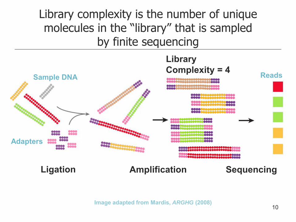
Library complexity is the number of unique molecules in the “library” that is sampled
by finite sequencing
Image adapted from Mardis, ARGHG (2008)
Ligation Amplification Sequencing
Sample DNA
Adapters
Reads
Library Complexity = 4
4
Modeling approach
• Assume we have C unique molecules in the library and we obtain N sequencing reads
• The probability distribution of the number of times we sequence a particular molecule is binomial (individual success probability p=1/C, N trials in total)
• Assume Poisson sampling as a tractable approximation (rate λ = N/C)
• Finally, truncate the Poisson process: we only see events that happened between L and R times (we don’t know how many molecules were observed 0 times)
See e.g. Cohen, JASA (1954) 5
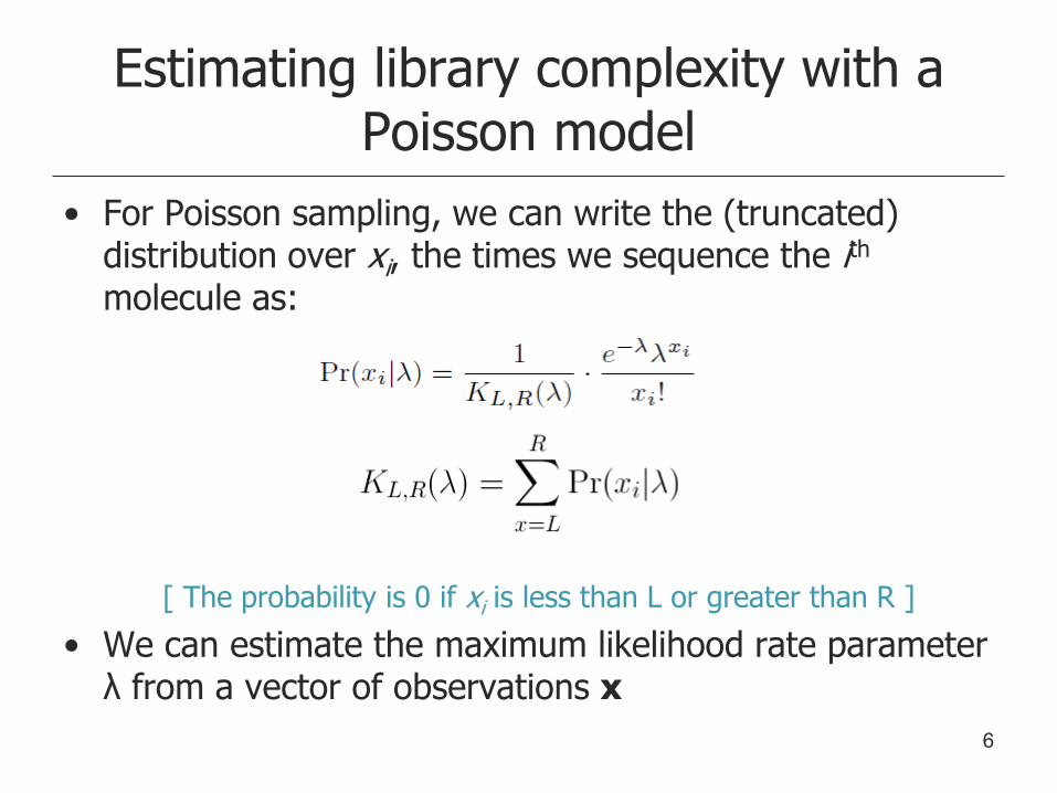
Estimating library complexity with a Poisson model
• For Poisson sampling, we can write the (truncated) distribution over xi, the times we sequence the ith molecule as:
[ The probability is 0 if xi is less than L or greater than R ]
• We can estimate the maximum likelihood rate parameter λ from a vector of observations x
6
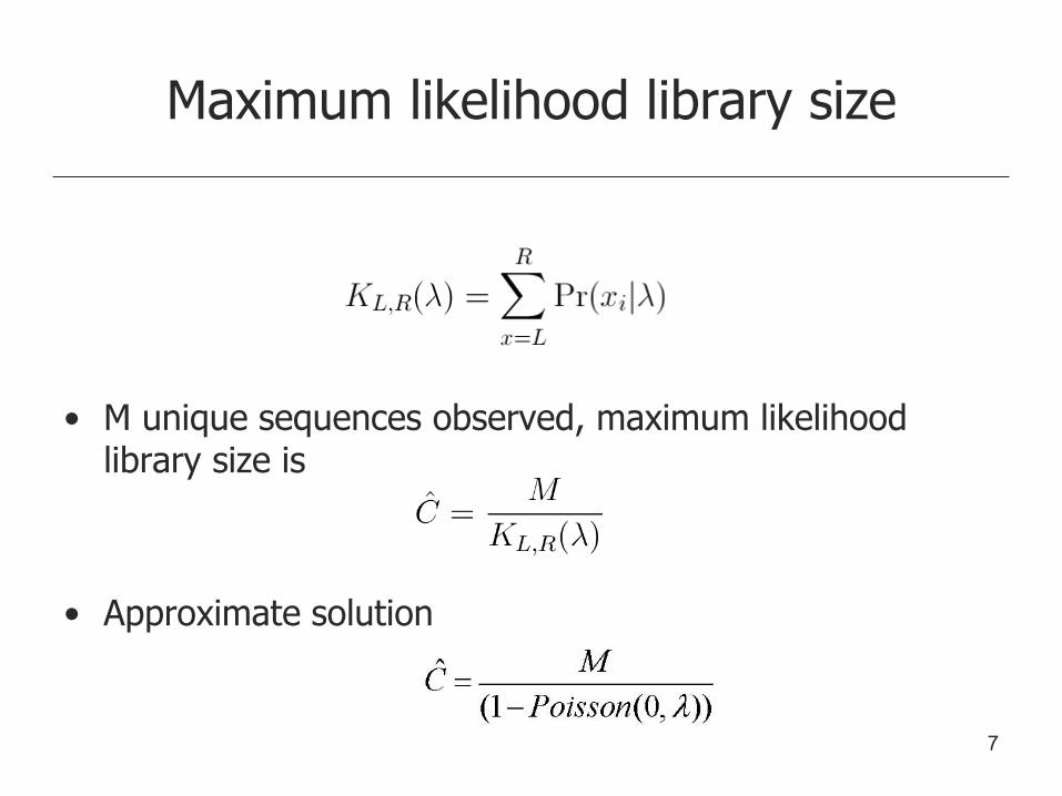
Maximum likelihood library size
• M unique sequences observed, maximum likelihood library size is
• Approximate solution
7
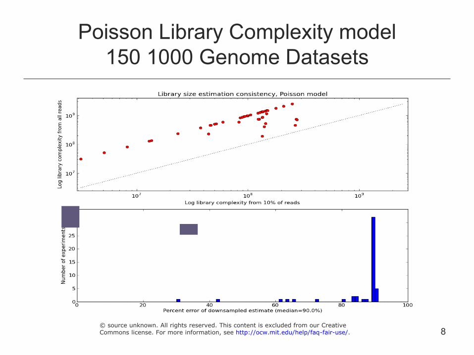
Poisson Library Complexity model 150 1000 Genome Datasets
8 © source unknown. All rights reserved. This content is excluded from our CreativeCommons license. For more information, see http://ocw.mit.edu/help/faq-fair-use/.
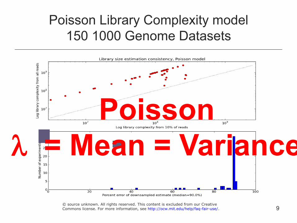
Poisson Library Complexity model 150 1000 Genome Datasets
Poisson l = Mean = Variance
9 © source unknown. All rights reserved. This content is excluded from our CreativeCommons license. For more information, see http://ocw.mit.edu/help/faq-fair-use/.
Library complexity is the number of unique molecules in the “library” that is sampled
by finite sequencing
Image adapted from Mardis, ARGHG (2008)
Ligation Amplification Sequencing
Sample DNA
Adapters
Reads
Library Complexity = 4
10
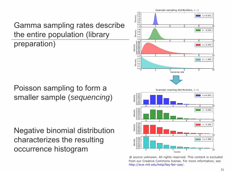
Gamma sampling rates describe the entire population (library preparation) Poisson sampling to form a smaller sample (sequencing) Negative binomial distribution characterizes the resulting occurrence histogram
11
@ source unknown. All rights reserved. This content is excludedfrom our Creative Commons license. For more information, seehttp://ocw.mit.edu/help/faq-fair-use/.
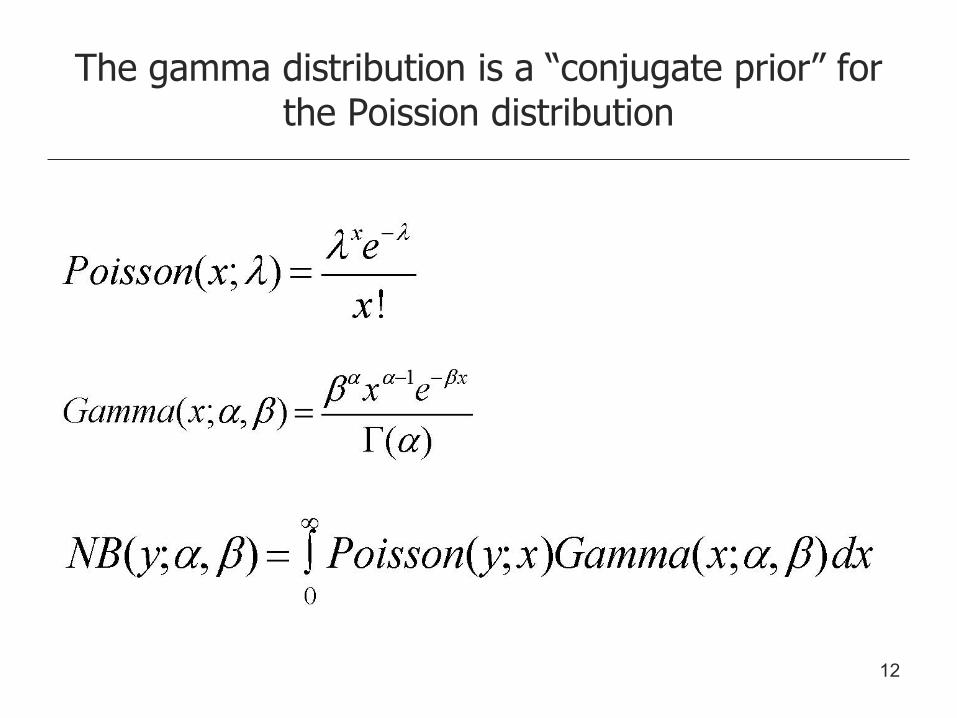
The gamma distribution is a “conjugate prior” for the Poission distribution
12
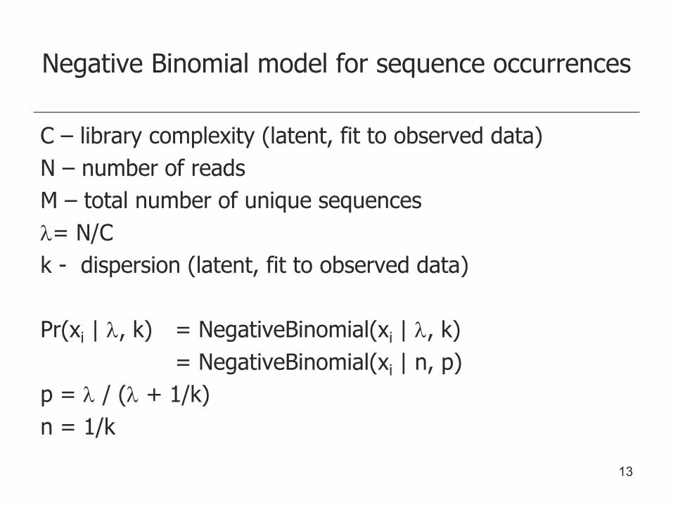
Negative Binomial model for sequence occurrences
C – library complexity (latent, fit to observed data)
N – number of reads
M – total number of unique sequences
l= N/C
k - dispersion (latent, fit to observed data)
Pr(xi | l, k) = NegativeBinomial(xi | l, k)
= NegativeBinomial(xi | n, p)
p = l / (l + 1/k)
n = 1/k
13
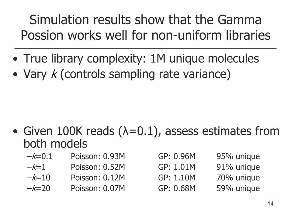
• True library complexity: 1M unique molecules
• Vary k (controls sampling rate variance)
• Given 100K reads (λ=0.1), assess estimates from both models –k=0.1 Poisson: 0.93M GP: 0.96M 95% unique
–k=1 Poisson: 0.52M GP: 1.01M 91% unique
–k=10 Poisson: 0.12M GP: 1.10M 70% unique
–k=20 Poisson: 0.07M GP: 0.68M 59% unique
Simulation results show that the Gamma Possion works well for non-uniform libraries
14
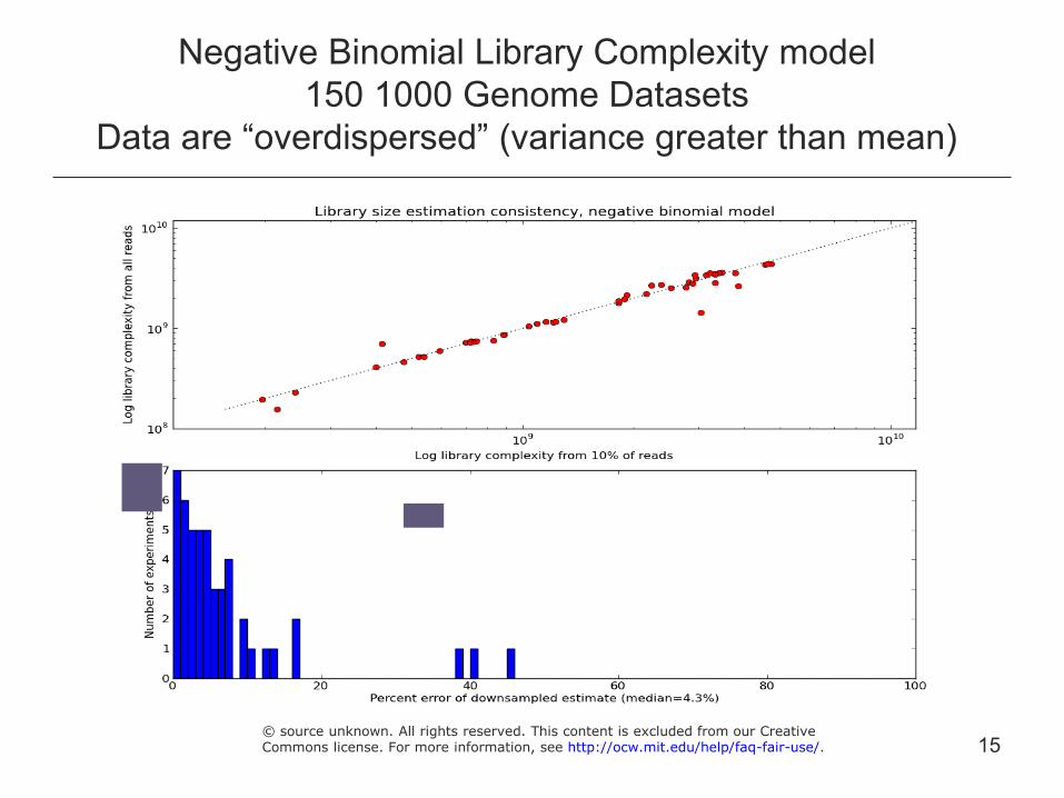
Negative Binomial Library Complexity model 150 1000 Genome Datasets
Data are “overdispersed” (variance greater than mean)
15 © source unknown. All rights reserved. This content is excluded from our CreativeCommons license. For more information, see http://ocw.mit.edu/help/faq-fair-use/.
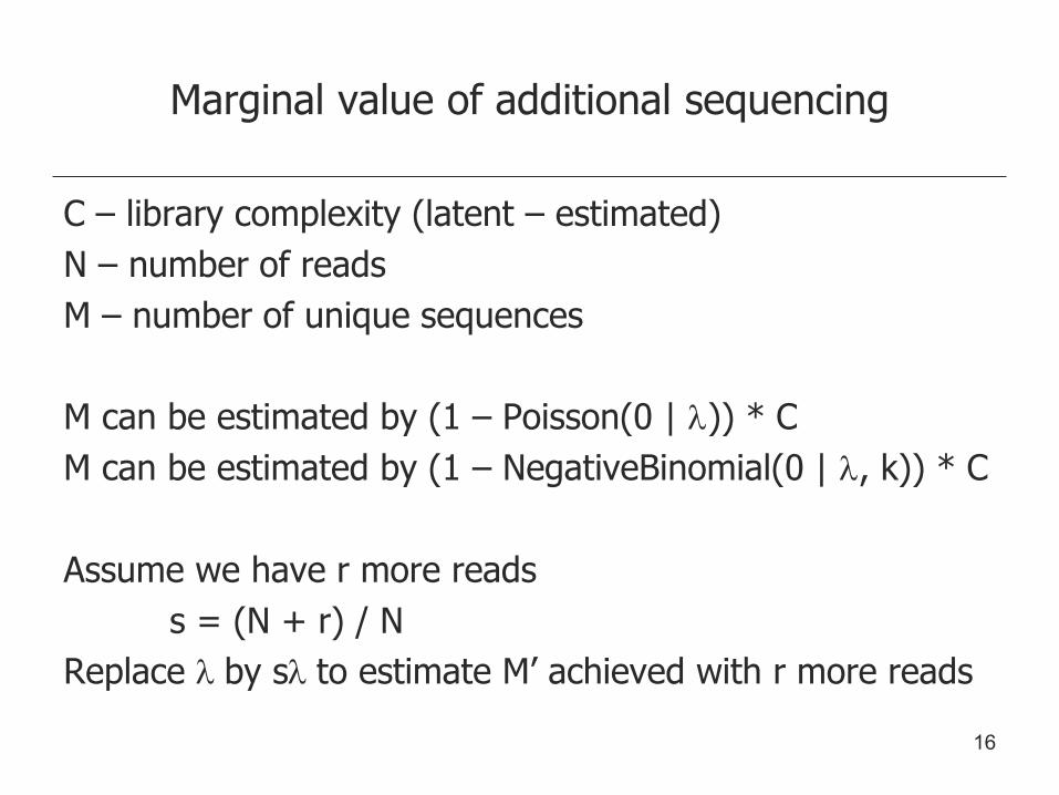
Marginal value of additional sequencing
C – library complexity (latent – estimated)
N – number of reads
M – number of unique sequences
M can be estimated by (1 – Poisson(0 | l)) * C
M can be estimated by (1 – NegativeBinomial(0 | l, k)) * C
Assume we have r more reads
s = (N + r) / N
Replace l by sl to estimate M’ achieved with r more reads
16
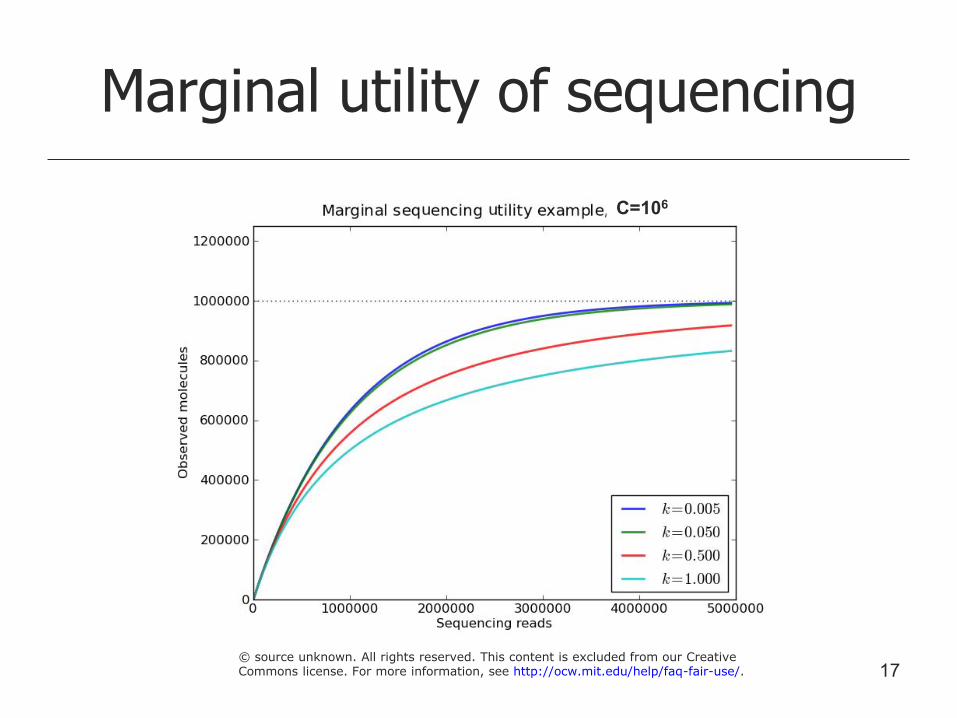
Marginal utility of sequencing
C=106
17 © source unknown. All rights reserved. This content is excluded from our CreativeCommons license. For more information, see http://ocw.mit.edu/help/faq-fair-use/.

Lecture 5 – Libraries and Indexing
• Library Complexity
– How do we estimate the complexity of a sequencing library?
• Full-text Minute-size index (FM Index/BWT)
– How do we convert a genome into an alternate representation that permits rapid matching of millions of sequence reads?
• Read Alignment
– How can we use an FM index and BWT to rapidly align reads to a reference genome?
18
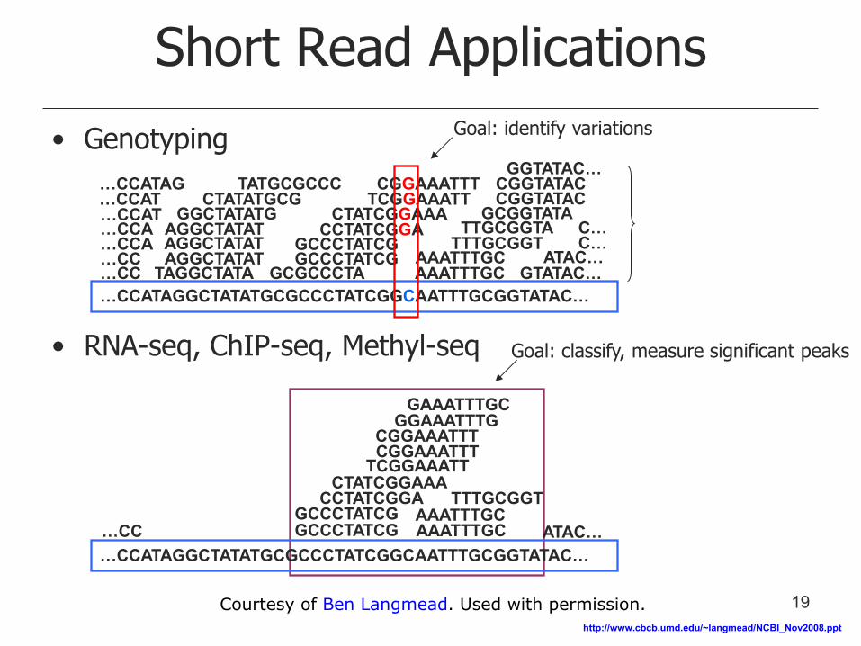
Short Read Applications
• Genotyping
• RNA-seq, ChIP-seq, Methyl-seq
…CCATAGGCTATATGCGCCCTATCGGCAATTTGCGGTATAC… GCGCCCTA
GCCCTATCG GCCCTATCG
CCTATCGGA CTATCGGAAA
AAATTTGC AAATTTGC
TTTGCGGT TTGCGGTA
GCGGTATA
GTATAC…
TCGGAAATT CGGAAATTT
CGGTATAC
TAGGCTATA
GCCCTATCG GCCCTATCG
CCTATCGGA CTATCGGAAA
AAATTTGC AAATTTGC
TTTGCGGT
TCGGAAATT CGGAAATTT CGGAAATTT
AGGCTATAT AGGCTATAT AGGCTATAT
GGCTATATG CTATATGCG
…CC …CC …CCA …CCA …CCAT
ATAC… C… C…
…CCAT …CCATAG TATGCGCCC
GGTATAC… CGGTATAC
GGAAATTTG
…CCATAGGCTATATGCGCCCTATCGGCAATTTGCGGTATAC… ATAC… …CC
GAAATTTGC
Goal: identify variations
Goal: classify, measure significant peaks
http://www.cbcb.umd.edu/~langmead/NCBI_Nov2008.ppt
19 Courtesy of Ben Langmead. Used with permission.
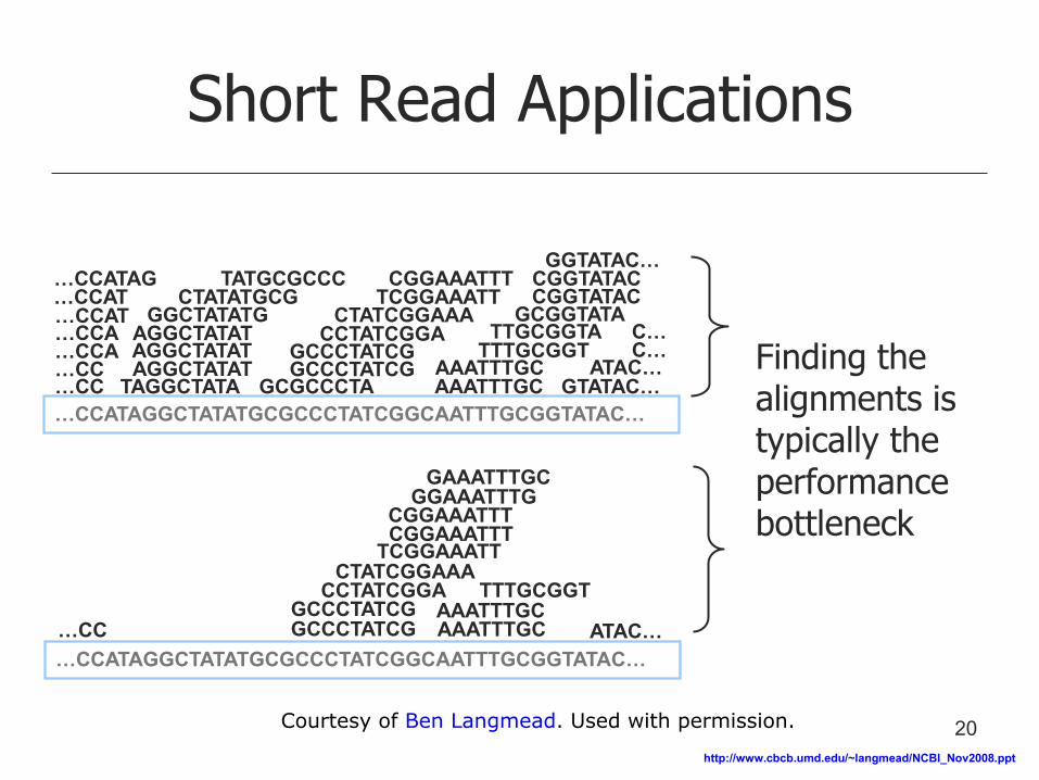
Short Read Applications
Finding the alignments is typically the performance bottleneck
…CCATAGGCTATATGCGCCCTATCGGCAATTTGCGGTATAC… GCGCCCTA
GCCCTATCG GCCCTATCG
CCTATCGGA CTATCGGAAA
AAATTTGC AAATTTGC
TTTGCGGT TTGCGGTA
GCGGTATA
GTATAC…
TCGGAAATT CGGAAATTT
CGGTATAC
TAGGCTATA
GCCCTATCG GCCCTATCG
CCTATCGGA CTATCGGAAA
AAATTTGC AAATTTGC
TTTGCGGT
TCGGAAATT CGGAAATTT CGGAAATTT
AGGCTATAT AGGCTATAT AGGCTATAT
GGCTATATG CTATATGCG
…CC …CC …CCA …CCA …CCAT
ATAC… C… C…
…CCAT …CCATAG TATGCGCCC
GGTATAC… CGGTATAC
GGAAATTTG
…CCATAGGCTATATGCGCCCTATCGGCAATTTGCGGTATAC… ATAC… …CC
GAAATTTGC
http://www.cbcb.umd.edu/~langmead/NCBI_Nov2008.ppt
20 Courtesy of Ben Langmead. Used with permission.
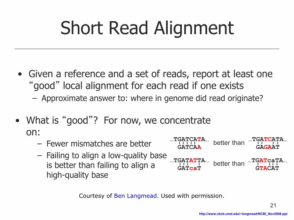
Short Read Alignment
• Given a reference and a set of reads, report at least one “good” local alignment for each read if one exists
– Approximate answer to: where in genome did read originate?
…TGATCATA…
GATCAA
…TGATCATA…
GAGAAT better than
• What is “good”? For now, we concentrate on:
…TGATATTA…
GATcaT
…TGATcaTA…
GTACAT better than
– Fewer mismatches are better
– Failing to align a low-quality base is better than failing to align a high-quality base
http://www.cbcb.umd.edu/~langmead/NCBI_Nov2008.ppt
21
Courtesy of Ben Langmead. Used with permission.
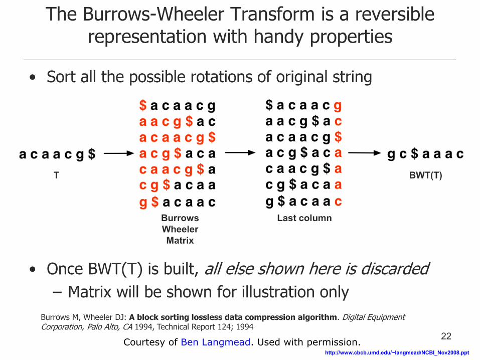
The Burrows-Wheeler Transform is a reversible representation with handy properties
• Sort all the possible rotations of original string
• Once BWT(T) is built, all else shown here is discarded
– Matrix will be shown for illustration only
Burrows Wheeler Matrix
Last column
BWT(T) T
Burrows M, Wheeler DJ: A block sorting lossless data compression algorithm. Digital Equipment Corporation, Palo Alto, CA 1994, Technical Report 124; 1994
http://www.cbcb.umd.edu/~langmead/NCBI_Nov2008.ppt
22 Courtesy of Ben Langmead. Used with permission.

A text occurrence has the same rank in the first and last columns
• When we rotate left and sort, the first character retains its rank. Thus the same text occurrence of a character has the same rank in the Last and First columns.
T
BWT(T)
Burrows Wheeler Matrix
Rank: 2
Rank: 2
http://www.cbcb.umd.edu/~langmead/NCBI_Nov2008.ppt
23 Courtesy of Ben Langmead. Used with permission.
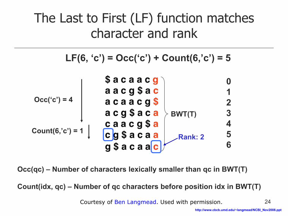
The Last to First (LF) function matches character and rank
BWT(T)
Rank: 2
http://www.cbcb.umd.edu/~langmead/NCBI_Nov2008.ppt
LF(6, ‘c’) = Occ(‘c’) + Count(6,’c’) = 5
Occ(‘c’) = 4
Count(6,’c’) = 1
Occ(qc) – Number of characters lexically smaller than qc in BWT(T) Count(idx, qc) – Number of qc characters before position idx in BWT(T)
0 1 2 3 4 5 6
24 Courtesy of Ben Langmead. Used with permission.
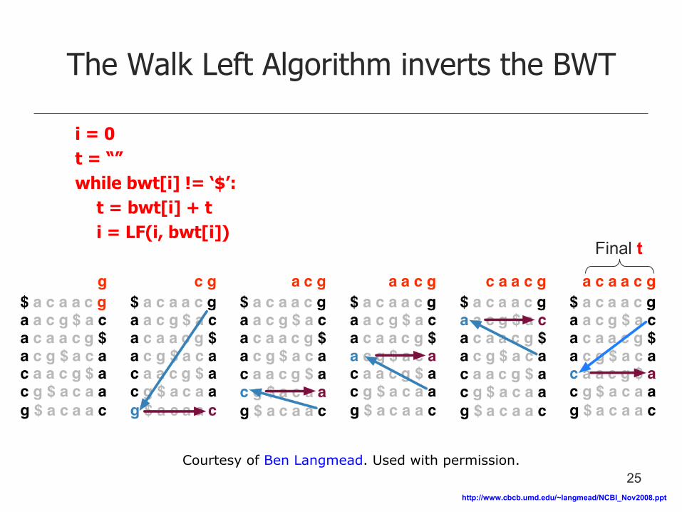
The Walk Left Algorithm inverts the BWT
i = 0
t = “”
while bwt[i] != ‘$’:
t = bwt[i] + t
i = LF(i, bwt[i]) Final t
http://www.cbcb.umd.edu/~langmead/NCBI_Nov2008.ppt
25 Courtesy of Ben Langmead. Used with permission.
Lecture 5 – Libraries and Indexing
• Library Complexity
– How do we estimate the complexity of a sequencing library?
• Full-text Minute-size index (FM Index/BWT)
– How do we convert a genome into an alternate representation that permits rapid matching of millions of sequence reads?
• Read Alignment
– How can we use an FM index and BWT to rapidly align reads to a reference genome?
26
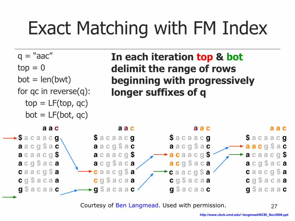
Exact Matching with FM Index
q = “aac”
top = 0
bot = len(bwt)
for qc in reverse(q):
top = LF(top, qc)
bot = LF(bot, qc)
http://www.cbcb.umd.edu/~langmead/NCBI_Nov2008.ppt
In each iteration top & bot delimit the range of rows beginning with progressively longer suffixes of q
27 Courtesy of Ben Langmead. Used with permission.
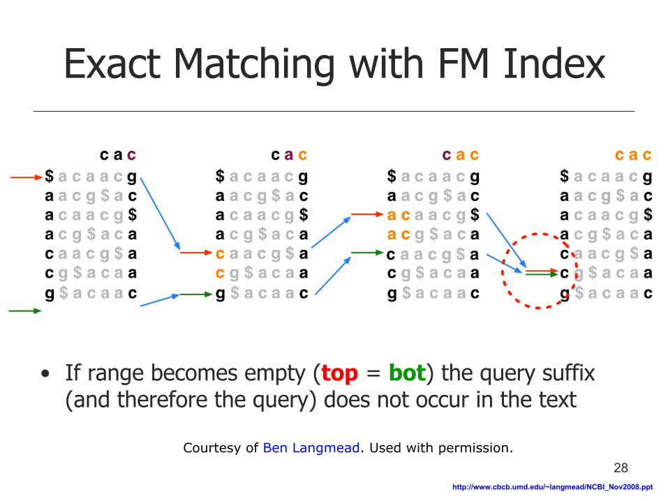
Exact Matching with FM Index
• If range becomes empty (top = bot) the query suffix (and therefore the query) does not occur in the text
http://www.cbcb.umd.edu/~langmead/NCBI_Nov2008.ppt
28 Courtesy of Ben Langmead. Used with permission.
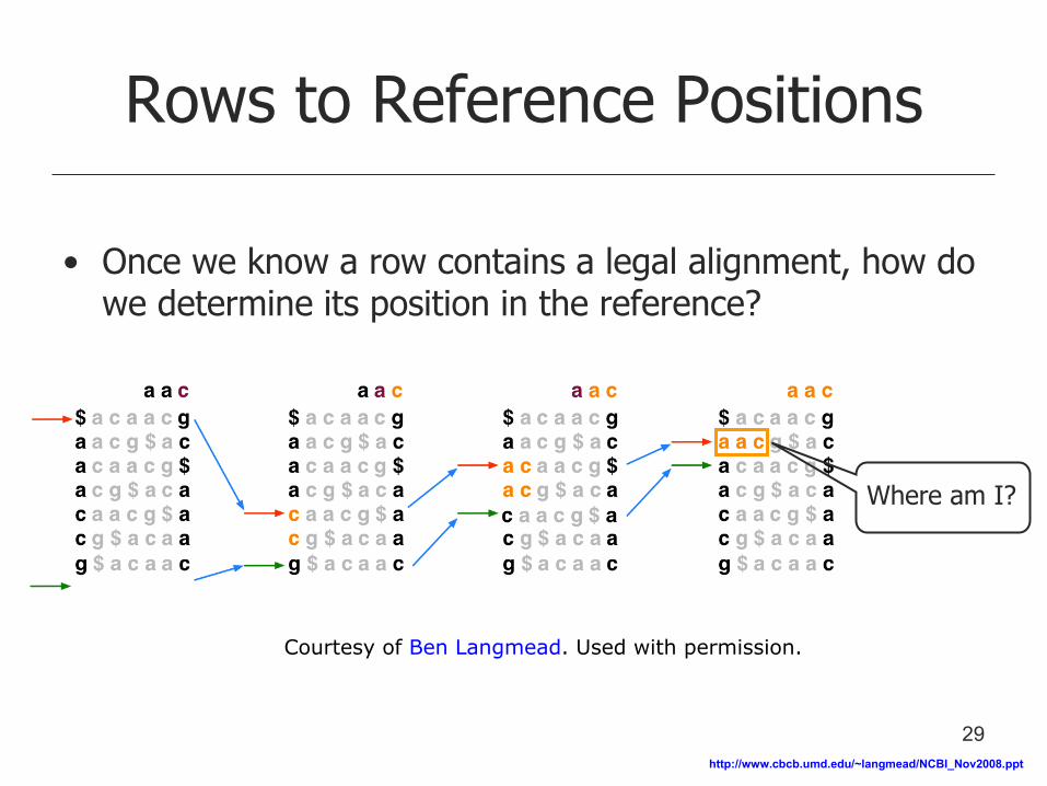
Rows to Reference Positions
• Once we know a row contains a legal alignment, how do we determine its position in the reference?
Where am I?
http://www.cbcb.umd.edu/~langmead/NCBI_Nov2008.ppt
29
Courtesy of Ben Langmead. Used with permission.
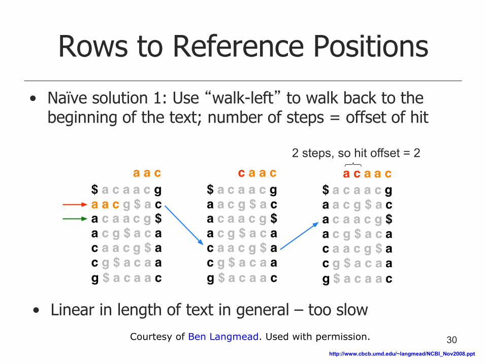
Rows to Reference Positions
• Naïve solution 1: Use “walk-left” to walk back to the beginning of the text; number of steps = offset of hit
• Linear in length of text in general – too slow
2 steps, so hit offset = 2
http://www.cbcb.umd.edu/~langmead/NCBI_Nov2008.ppt
30 Courtesy of Ben Langmead. Used with permission.
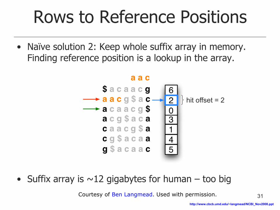
• Naïve solution 2: Keep whole suffix array in memory. Finding reference position is a lookup in the array.
• Suffix array is ~12 gigabytes for human – too big
Rows to Reference Positions
hit offset = 2
http://www.cbcb.umd.edu/~langmead/NCBI_Nov2008.ppt
31 Courtesy of Ben Langmead. Used with permission.
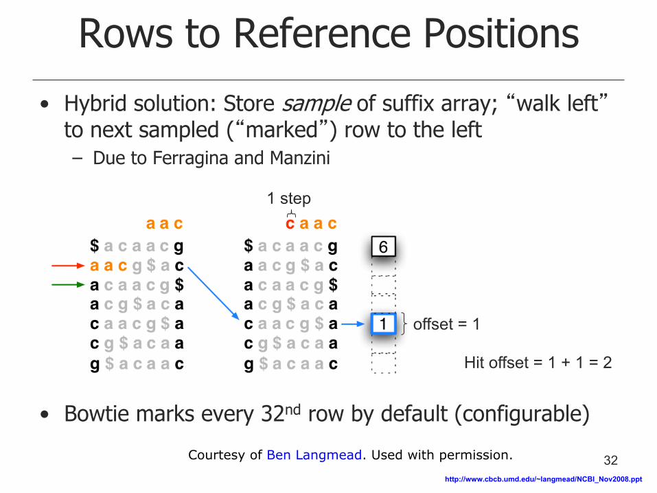
• Hybrid solution: Store sample of suffix array; “walk left” to next sampled (“marked”) row to the left
– Due to Ferragina and Manzini
• Bowtie marks every 32nd row by default (configurable)
Rows to Reference Positions
1 step
offset = 1
Hit offset = 1 + 1 = 2
http://www.cbcb.umd.edu/~langmead/NCBI_Nov2008.ppt
32 Courtesy of Ben Langmead. Used with permission.
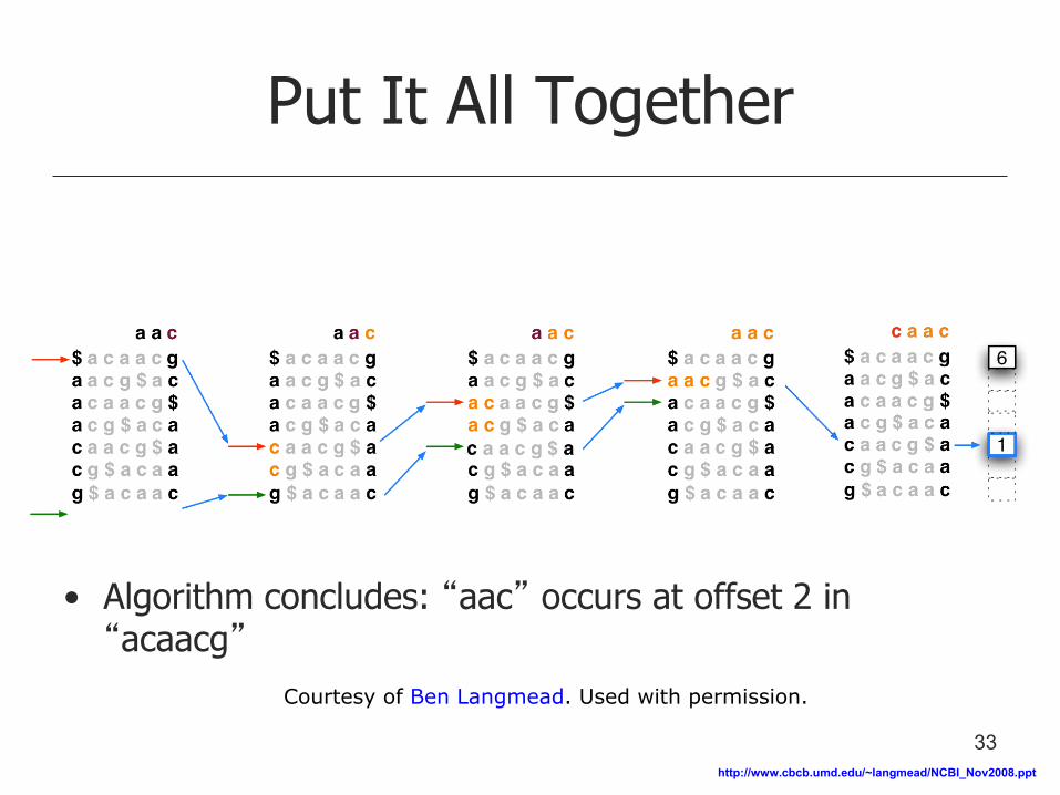
• Algorithm concludes: “aac” occurs at offset 2 in “acaacg”
Put It All Together
http://www.cbcb.umd.edu/~langmead/NCBI_Nov2008.ppt
33
Courtesy of Ben Langmead. Used with permission.
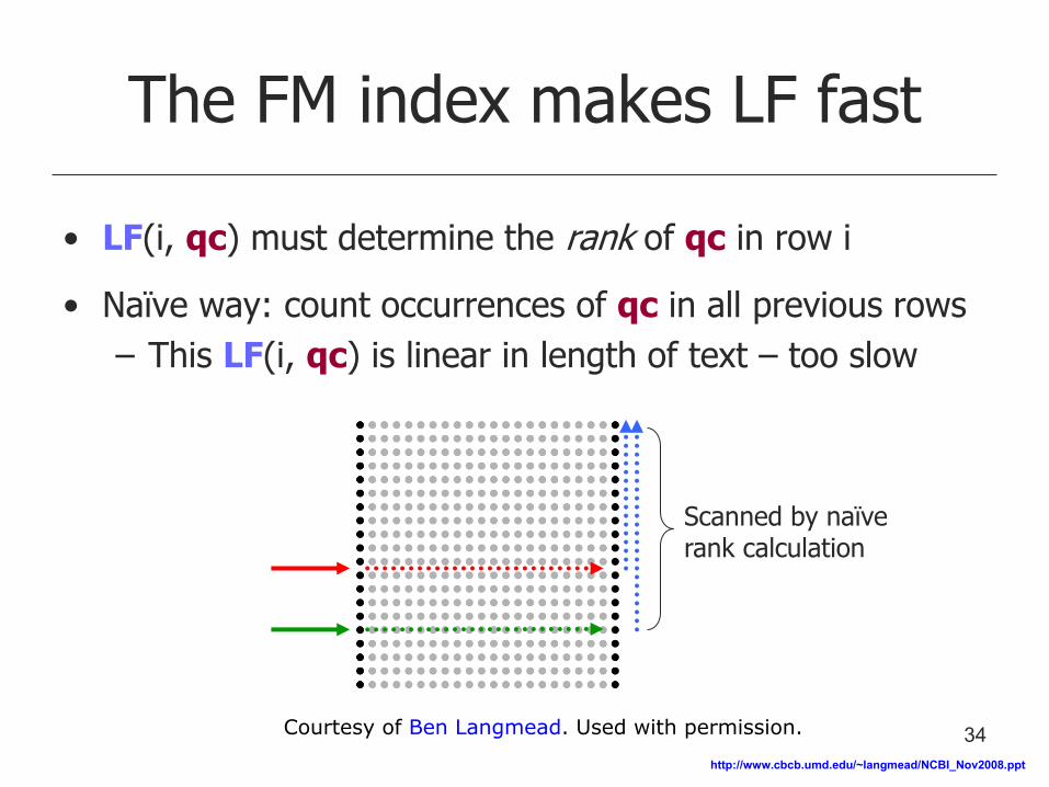
The FM index makes LF fast
• LF(i, qc) must determine the rank of qc in row i
• Naïve way: count occurrences of qc in all previous rows
– This LF(i, qc) is linear in length of text – too slow
Scanned by naïve rank calculation
http://www.cbcb.umd.edu/~langmead/NCBI_Nov2008.ppt
34 Courtesy of Ben Langmead. Used with permission.
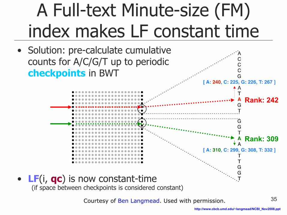
A Full-text Minute-size (FM) index makes LF constant time
• Solution: pre-calculate cumulative counts for A/C/G/T up to periodic checkpoints in BWT
• LF(i, qc) is now constant-time (if space between checkpoints is considered constant)
Rank: 309
Rank: 242
http://www.cbcb.umd.edu/~langmead/NCBI_Nov2008.ppt
35 Courtesy of Ben Langmead. Used with permission.
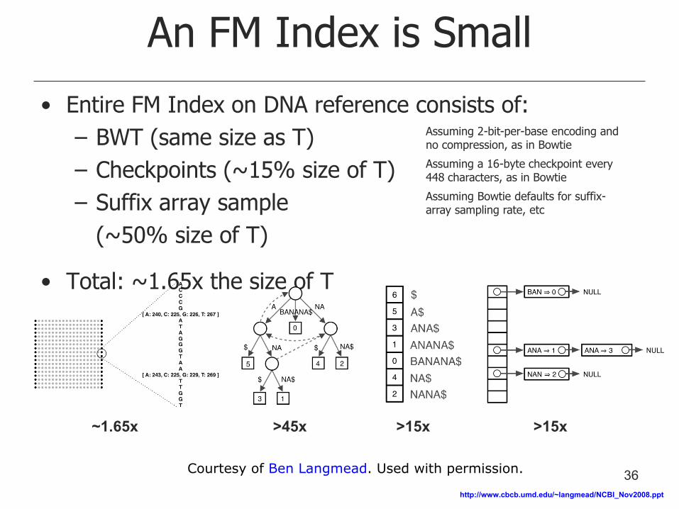
An FM Index is Small
• Entire FM Index on DNA reference consists of:
– BWT (same size as T)
– Checkpoints (~15% size of T)
– Suffix array sample
(~50% size of T)
• Total: ~1.65x the size of T
>45x >15x >15x ~1.65x
Assuming 2-bit-per-base encoding and no compression, as in Bowtie
Assuming a 16-byte checkpoint every 448 characters, as in Bowtie
Assuming Bowtie defaults for suffix-array sampling rate, etc
http://www.cbcb.umd.edu/~langmead/NCBI_Nov2008.ppt
36 Courtesy of Ben Langmead. Used with permission.
FM Index in Bioinformatics
• Oligomer counting
– Healy J et al: Annotating large genomes with exact word matches. Genome Res 2003, 13(10):2306-2315.
• Whole-genome alignment
– Li H et al: Fast and accurate short read alignment with Burrows-Wheeler transform Bioinformatics 2009, 25(14):1754-1760.
BWA Aligner
– Lippert RA: Space-efficient whole genome comparisons with Burrows-Wheeler transforms. J Comp Bio 2005, 12(4):407-415.
• Smith-Waterman alignment to large reference
– Lam TW et al: Compressed indexing and local alignment of DNA. Bioinformatics 2008, 24(6):791-797.
http://www.cbcb.umd.edu/~langmead/NCBI_Nov2008.ppt 37 Courtesy of Ben Langmead. Used with permission.
Short Read Alignment
• FM Index finds exact sequence matches quickly in small memory, but short read alignment demands more:
– Allowances for mismatches
– Consideration of quality values
• Bowtie’s solution: backtracking quality-aware search
http://www.cbcb.umd.edu/~langmead/NCBI_Nov2008.ppt
38
Courtesy of Ben Langmead. Used with permission.
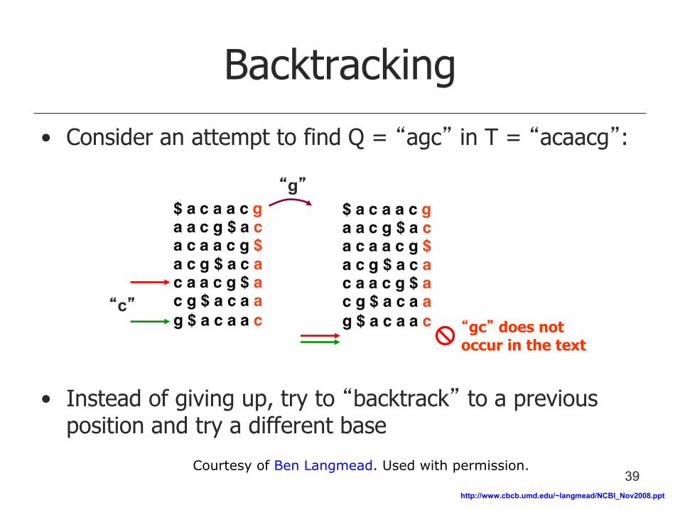
Backtracking
• Consider an attempt to find Q = “agc” in T = “acaacg”:
• Instead of giving up, try to “backtrack” to a previous position and try a different base
“gc” does not occur in the text
“g”
“c”
http://www.cbcb.umd.edu/~langmead/NCBI_Nov2008.ppt
39 Courtesy of Ben Langmead. Used with permission.
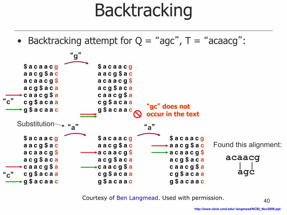
Backtracking
Found this alignment:
acaacg
agc
“g”
“a” “a”
“c”
“c”
• Backtracking attempt for Q = “agc”, T = “acaacg”:
“gc” does not occur in the text
Substitution
http://www.cbcb.umd.edu/~langmead/NCBI_Nov2008.ppt
40 Courtesy of Ben Langmead. Used with permission.
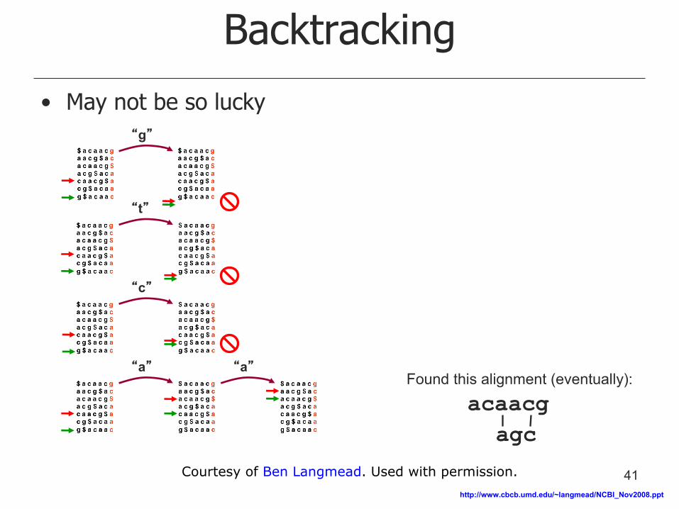
Backtracking
• May not be so lucky
Found this alignment (eventually):
acaacg
agc
“g”
“t”
“c”
“a” “a”
http://www.cbcb.umd.edu/~langmead/NCBI_Nov2008.ppt
41 Courtesy of Ben Langmead. Used with permission.
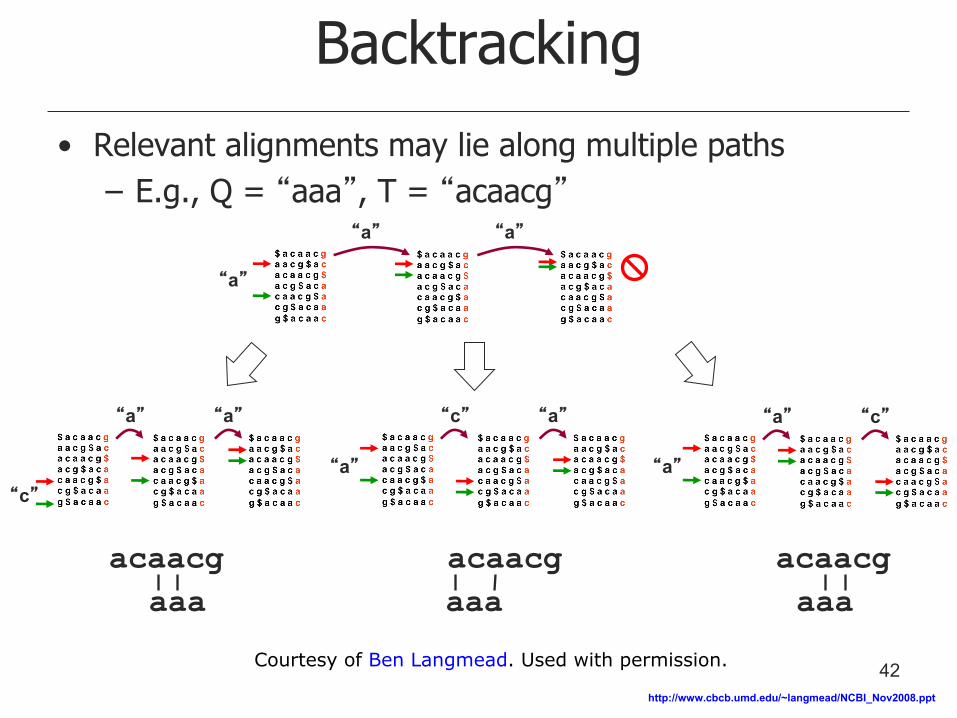
Backtracking
• Relevant alignments may lie along multiple paths
– E.g., Q = “aaa”, T = “acaacg”
acaacg
aaa
“a” “a”
acaacg
aaa
acaacg
aaa
“a” “c” “c” “a”
“a”
“a” “c”
“a” “a”
“a”
http://www.cbcb.umd.edu/~langmead/NCBI_Nov2008.ppt
42 Courtesy of Ben Langmead. Used with permission.
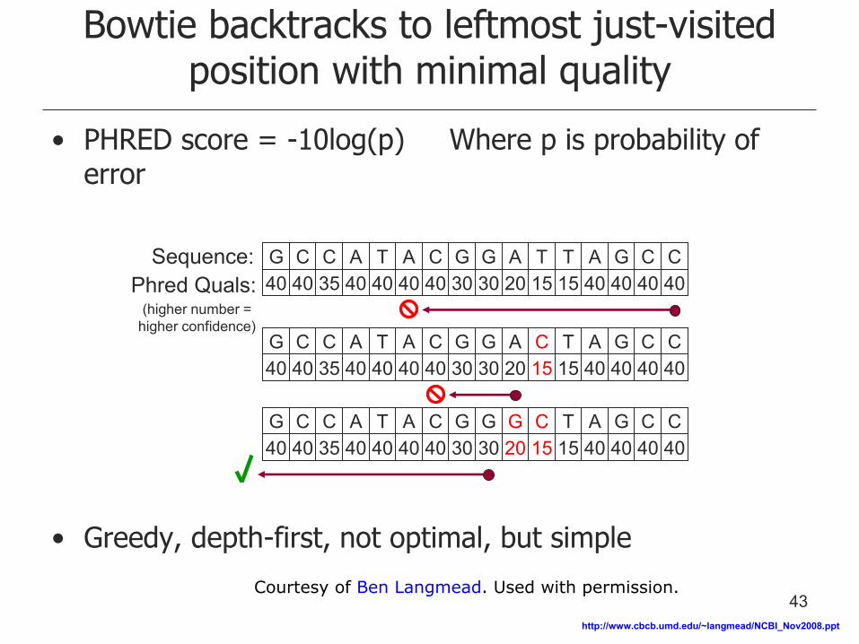
Bowtie backtracks to leftmost just-visited position with minimal quality
• PHRED score = -10log(p) Where p is probability of error
• Greedy, depth-first, not optimal, but simple
Sequence: Phred Quals:
(higher number = higher confidence)
G C C A T A C G G A T T A G C C 40 40 35 40 40 40 40 30 30 20 15 15 40 40 40 40
G C C A T A C G G A C T A G C C 40 40 35 40 40 40 40 30 30 20 15 15 40 40 40 40
G C C A T A C G G G C T A G C C 40 40 35 40 40 40 40 30 30 20 15 15 40 40 40 40
http://www.cbcb.umd.edu/~langmead/NCBI_Nov2008.ppt
43 Courtesy of Ben Langmead. Used with permission.
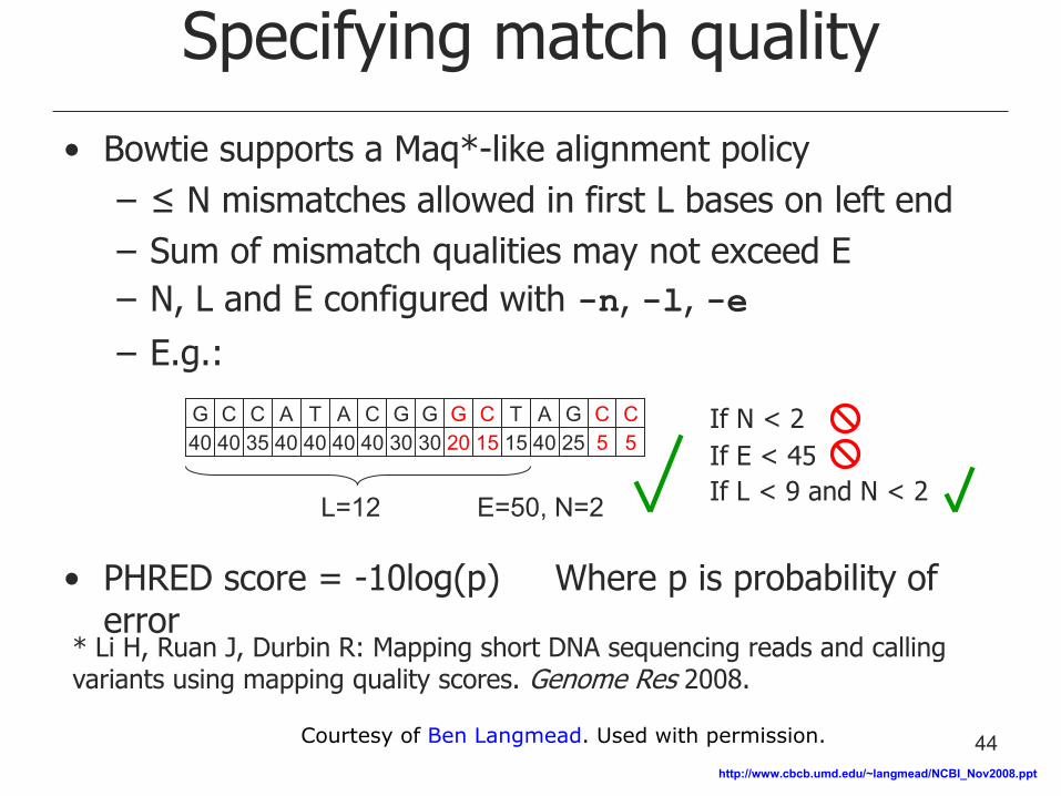
Specifying match quality
• Bowtie supports a Maq*-like alignment policy
– ≤ N mismatches allowed in first L bases on left end
– Sum of mismatch qualities may not exceed E
– N, L and E configured with -n, -l, -e
– E.g.:
• PHRED score = -10log(p) Where p is probability of error
* Li H, Ruan J, Durbin R: Mapping short DNA sequencing reads and calling variants using mapping quality scores. Genome Res 2008.
G C C A T A C G G G C T A G C C 40 40 35 40 40 40 40 30 30 20 15 15 40 25 5 5
L=12 E=50, N=2
If N < 2
If E < 45
If L < 9 and N < 2
http://www.cbcb.umd.edu/~langmead/NCBI_Nov2008.ppt
44 Courtesy of Ben Langmead. Used with permission.
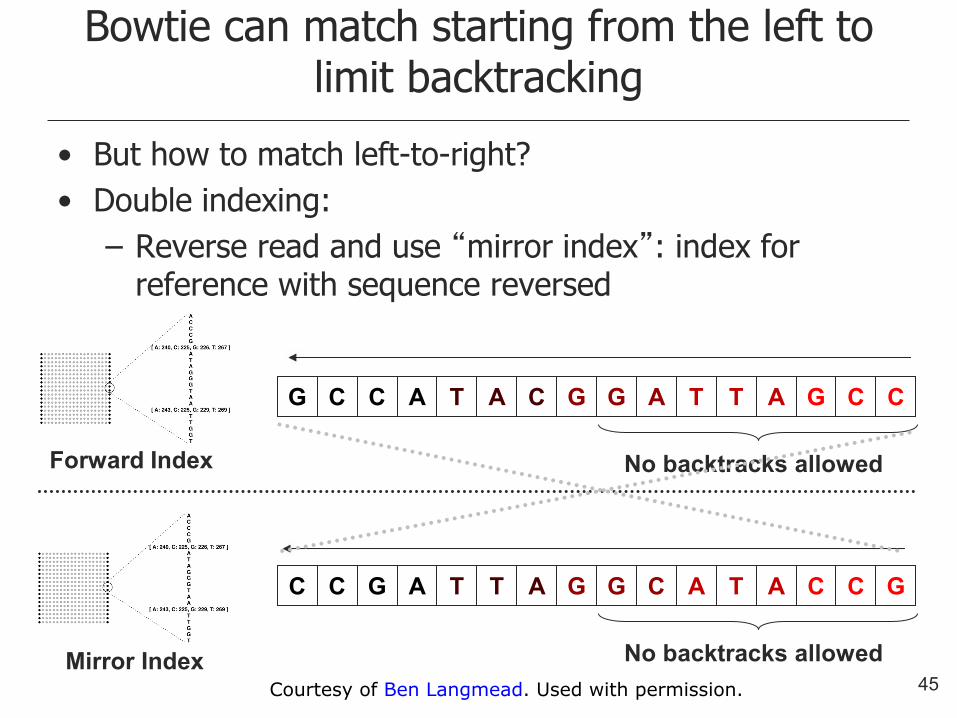
Bowtie can match starting from the left to limit backtracking
• But how to match left-to-right?
• Double indexing:
– Reverse read and use “mirror index”: index for reference with sequence reversed
G C C A T A C G G A T T A G C C
C C G A T T A G G C A T A C C G
No backtracks allowed
Forward Index
Mirror Index
No backtracks allowed
45 Courtesy of Ben Langmead. Used with permission.
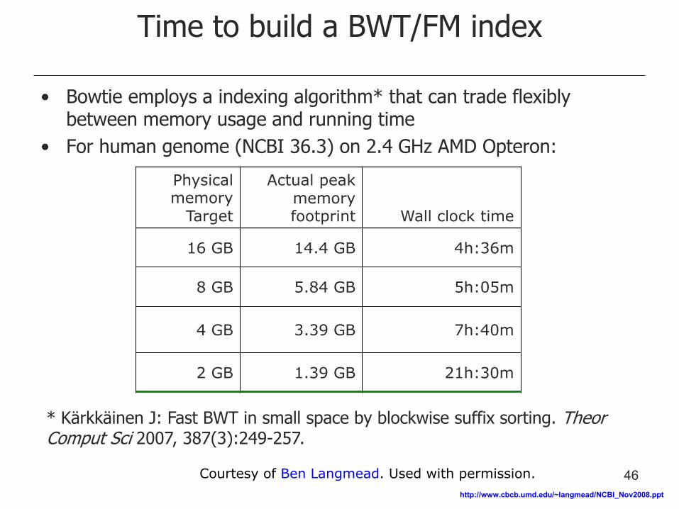
Time to build a BWT/FM index
• Bowtie employs a indexing algorithm* that can trade flexibly between memory usage and running time
• For human genome (NCBI 36.3) on 2.4 GHz AMD Opteron:
* Kärkkäinen J: Fast BWT in small space by blockwise suffix sorting. Theor Comput Sci 2007, 387(3):249-257.
Physical memory
Target
Actual peak memory footprint Wall clock time
16 GB 14.4 GB 4h:36m
8 GB 5.84 GB 5h:05m
4 GB 3.39 GB 7h:40m
2 GB 1.39 GB 21h:30m
http://www.cbcb.umd.edu/~langmead/NCBI_Nov2008.ppt
46 Courtesy of Ben Langmead. Used with permission.
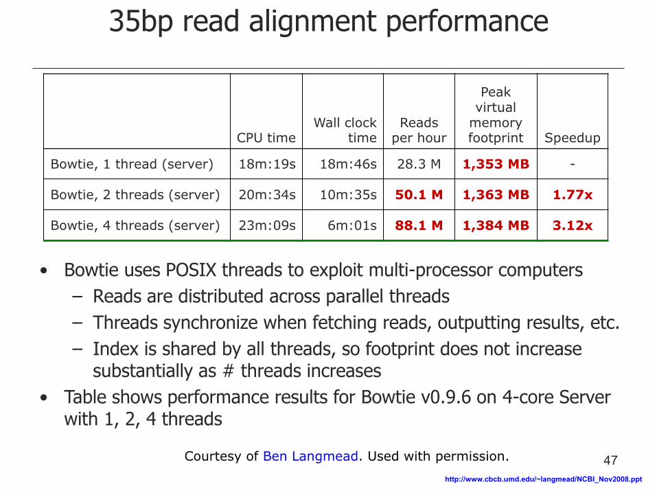
35bp read alignment performance
CPU time Wall clock
time Reads
per hour
Peak virtual
memory footprint Speedup
Bowtie, 1 thread (server) 18m:19s 18m:46s 28.3 M 1,353 MB -
Bowtie, 2 threads (server) 20m:34s 10m:35s 50.1 M 1,363 MB 1.77x
Bowtie, 4 threads (server) 23m:09s 6m:01s 88.1 M 1,384 MB 3.12x
• Bowtie uses POSIX threads to exploit multi-processor computers
– Reads are distributed across parallel threads
– Threads synchronize when fetching reads, outputting results, etc.
– Index is shared by all threads, so footprint does not increase substantially as # threads increases
• Table shows performance results for Bowtie v0.9.6 on 4-core Server with 1, 2, 4 threads
http://www.cbcb.umd.edu/~langmead/NCBI_Nov2008.ppt
47 Courtesy of Ben Langmead. Used with permission.
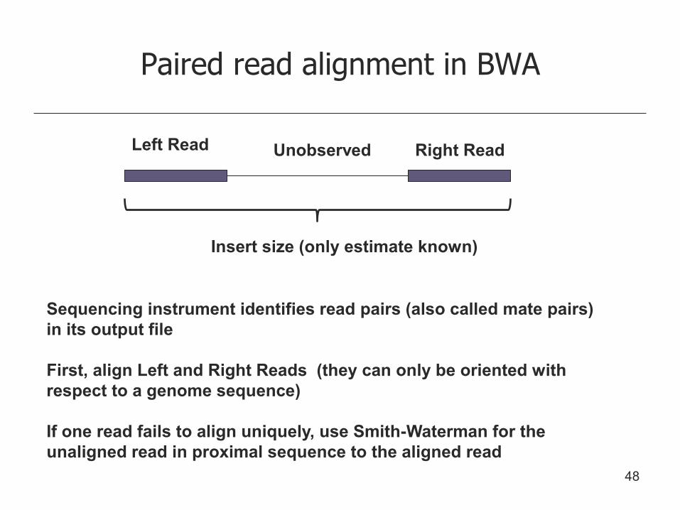
Paired read alignment in BWA
Left Read Right Read Unobserved
Insert size (only estimate known)
Sequencing instrument identifies read pairs (also called mate pairs) in its output file First, align Left and Right Reads (they can only be oriented with respect to a genome sequence) If one read fails to align uniquely, use Smith-Waterman for the unaligned read in proximal sequence to the aligned read
48
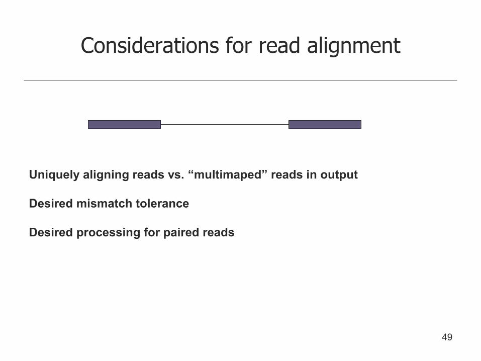
Considerations for read alignment
Uniquely aligning reads vs. “multimaped” reads in output Desired mismatch tolerance Desired processing for paired reads
49

FIN
50
MIT OpenCourseWarehttp://ocw.mit.edu
7.91J / 20.490J / 20.390J / 7.36J / 6.802J / 6.874J / HST.506J Foundations of Computational and Systems BiologySpring 2014
For information about citing these materials or our Terms of Use, visit: http://ocw.mit.edu/terms.