1 OF 17

Statistics 18_2_sample_t_test.pdf

Michael Hallstone, Ph.D. hallston@hawaii.edu

Lecture 18: Two-Sample Hypothesis Test of Means Some Common Sense Assumptions for Two Sample Hypothesis Tests

1. The test variable used is appropriate for a mean (interval/ratio level). (Hint for exam: no

student project should ever violate this nor have to assume it. Your data set will have this sort of variable.)

2. The data comes from a random sample. (Hint for exam: all student projects violate this assumption.)

3. The two samples are independent. Definition of "independence" from the book says, "A sample selected from the first population is said to be an independent sample if it isn't related in some way to the data source found in the second population." The sixth edition defines dependence as, “If the same (or related) data sources are used to generate the data sets for each population, then the samples taken from each population are said to be dependent.”

a. An example of two dependent samples would be any “before and after” type of test or measure, or if we were looking at the mean age between parents and children. By definition we know that a parent is older than their children. Also if we were looking at the mean age between husbands and wives, typically (not always) husbands tend to be older than their wives. In these two cases the samples are dependent.

b. (Hint for exam: you do not have to mention this assumption, most likely you are okay.)

4. Use the really good flow chart below first! If both sample sizes are greater than 30 (both n's >30) use Z distribution. If both populations are known to be "normal" you may use Z regardless of sample sizes. (However in practice if the populations are known to be normal and the sample sizes are small, not around 30, it is better to use the t distribution instead of Z -- it's more conservative.) If both n's <30 and populations are unknown we assume the populations are normal and use t distribution. Just make sure you follow the flow chart below.

a. So in plain English we now have two populations. When n is <30 in one or both samples we assume that the test variable is normally distributed in BOTH of the populations. If you test “mean age” for men and women then you have a population of men and population of women. You assume age is normally distributed in the population of men and the population of women. Hint for exam: if your n<30 in either or your samples you will make this assumption! Most likely your total sample size is not at least 60, so when you chop your spss data set sample into two groups, each of those n’s or sample sizes will NOT be greater than 30!) There is a sampling distribution of means for the population of men and a sampling distribution of means for the population of women. The only way that the each of these

2 OF 17

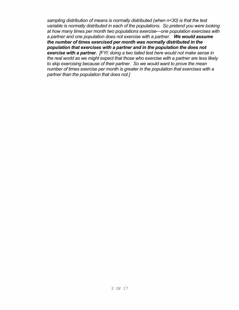
sampling distribution of means is normally distributed (when n<30) is that the test variable is normally distributed in each of the populations. So pretend you were looking at how many times per month two populations exercise—one population exercises with a partner and one population does not exercise with a partner. We would assume the number of times exercised per month was normally distributed in the population that exercises with a partner and in the population the does not exercise with a partner. [FYI: doing a two tailed test here would not make sense in the real world as we might expect that those who exercise with a partner are less likely to skip exercising because of their partner. So we would want to prove the mean number of times exercise per month is greater in the population that exercises with a partner than the population that does not.]

3 OF 17

Theory behind two sample hypothesis testing

Go back to sampling distribution of means and Central Limits Theorem. We know that sampling

distribution of means follows a normal distribution, clustered around the population mean. Applying

what we know about the probabilities associated with a normal distribution, 95.4% of the time the

sample mean will fall within plus or minus 2 standard deviations from the mean. That is true for two

samples as well.

4 OF 17

Assume there are two sampling distributions of means for two populations. You could take samples

from each and compute the differences in the two means. If you did that ad nausea then you would

have a sampling distribution of differences between means and all the stuff about normal distributions

would apply. See below for two diagrams of the “sampling distribution of differences of means.”

5 OF 17

What we do is we look at differences between the two means and see if they are equal to zero. If we

take random samples from each population and there really is no major differences between the two

population parameters, then we would expect the difference to be small (but unlikely to be zero due to

sampling variation). If there are actually true differences in the populations, we would expect the

differences to be large.

6 OF 17

Below is an image of the sampling distribution of means when µ1 ≠ µ2. or when µ1 − µ2≠ 0 . or

when. The bottom line is when µ1 ≠ µ2 we expect large differences between µ1 & µ2.

7 OF 17

Now when: µ1 = µ2 we expect small differences between µ1 & µ2 . See below.

Setting up null and alternative hypothesis for two sample t tests H0: µ1 − µ2 = 0 H1: µ1 − µ2 ≠ 0 or using algebra: H0: µ1 = µ2 H1: µ1 ≠ µ2

TR=σ xx

xx21

)( 21

−

− this is the formula when both n’s are greater than 30 and/or when one or both n’s are

less than 30 but we assume σσ2

2

2

1 =

new measure of dispersion: standard error of the differences of means

known pop.: σx bar 1 - x bar 2= nn 2

2

2

1

2

1 σσ +

8 OF 17

unknown pop: σx bar 1 - x bar 2= ns

ns

2

2

2

1

2

1 +

NOTE: there is a different formula when one or both samples are smaller than 30 and we assume

the populations have the same variance: σσ2

2

2

1 =

I shall be kind in this class to those computing data by hand and will not force you to do the

hypothesis test for:

H0: σσ2

2

2

1 = H1: σσ2

2

2

1 ≠

we simply assume that all students who have one or both n’s that are less than 30 have the following

situation: σσ2

2

2

1 ≠ This means for those computing the data by hand AND one or both n’s that are

less than 30 they should make this assumption and use:

ns

nsxx

2

2

2

1

2

1

21 )(

+

−

Setting up Null and Alternative Hypothesis

Setting up the null and alternative hypothesis for two sample tests not much different from one sample

tests. It is still sort of “bassackwards.” What you want to “prove” you put in the alternative hypothesis

and you “prove” it by rejecting its exact opposite. Kind of weird, but the best way to get over it is to

practice doing a whole bunch of them. For example say I want to prove that the population mean of

some variable (say age) of men is different than that of women (note I don’t care which way it’s

different!):

9 OF 17

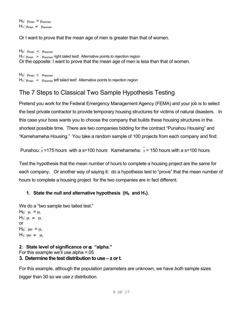
H0: µmen = µwomen H1: µmen ≠ µwomen Or I want to prove that the mean age of men is greater than that of women.

H0: µmen < µwomen H1: µmen > µwomen right tailed test! Alternative points to rejection region Or the opposite: I want to prove that the mean age of men is less than that of women.

H0: µmen > µwomen H1: µmen < µwomen left tailed test! Alternative points to rejection region The 7 Steps to Classical Two Sample Hypothesis Testing

Pretend you work for the Federal Emergency Management Agency (FEMA) and your job is to select

the best private contractor to provide temporary housing structures for victims of natural disasters. In

this case your boss wants you to choose the company that builds these housing structures in the

shortest possible time. There are two companies bidding for the contract “Punahou Housing” and

“Kamehameha Housing.” You take a random sample of 100 projects from each company and find:

Punahou: x =175 hours with a s=100 hours Kamehameha: x = 150 hours with a s=100 hours

Test the hypothesis that the mean number of hours to complete a housing project are the same for

each company. Or another way of saying it: do a hypothesis test to “prove” that the mean number of

hours to complete a housing project for the two companies are in fact different.

1. State the null and alternative hypothesis (H0 and H1).

We do a “two sample two tailed test.” H0: µ1 = µ2 H1: µ1 ≠ µ2

or H0: µP = µΚ H1: µP ≠ µΚ 2. State level of significance or α “alpha.” For this example we’ll use alpha =.05 3. Determine the test distribution to use – z or t.

For this example, although the population parameters are unknown, we have both sample sizes

bigger than 30 so we use z distribution.

10 OF 17

Note that when one or both of your n<30 there are two different formulas (the book calls them

“procedure 3” and “procedure 4”) depending upon whether or not the variances of your two variables

are equal. The book says the df are different for the two tests, but SPSS does it a little differently.

You may do what the book says or just use the same df for both formulas (df= n1 + n2 - 2). This

gives you a critical rejection value that is slightly less conservative, but the computer program

essentially does this so it can’t be that bad!

4. Define the rejection regions. And draw a picture!

In this case, we have two tailed test so we split the 5% up – ½ in each tail. That translates to

z(1.96)=.4750. Draw it out with both “acceptance regions” and “rejection regions.”

5. State the decision rule. Reject the null if the TR >1.96 or TR<-1.96, otherwise FTR.

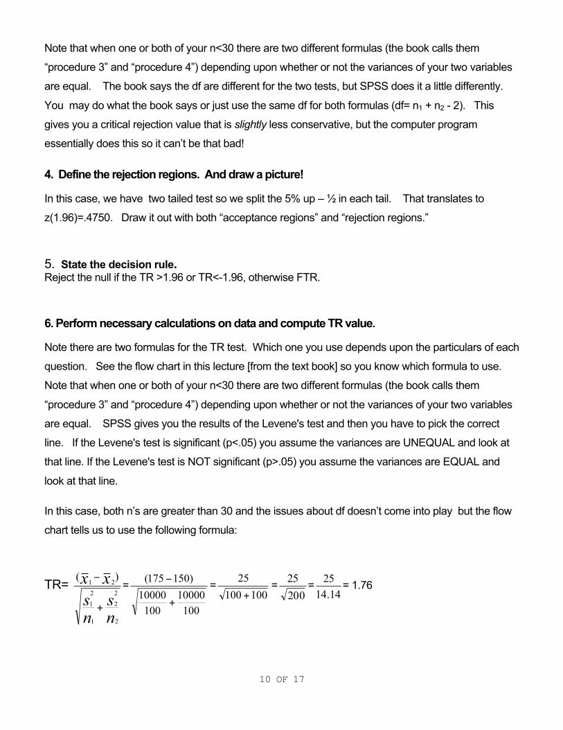
6. Perform necessary calculations on data and compute TR value.

Note there are two formulas for the TR test. Which one you use depends upon the particulars of each

question. See the flow chart in this lecture [from the text book] so you know which formula to use.

Note that when one or both of your n<30 there are two different formulas (the book calls them

“procedure 3” and “procedure 4”) depending upon whether or not the variances of your two variables

are equal. SPSS gives you the results of the Levene's test and then you have to pick the correct

line. If the Levene's test is significant (p<.05) you assume the variances are UNEQUAL and look at

that line. If the Levene's test is NOT significant (p>.05) you assume the variances are EQUAL and

look at that line.

In this case, both n’s are greater than 30 and the issues about df doesn’t come into play but the flow

chart tells us to use the following formula:

TR=

ns

nsxx

2

2

2

1

2

1

21 )(

+

−=

10010000

10010000

)150175(

+

− =100100

25+

=20025 =

14.1425 = 1.76

11 OF 17

7. Compare TR value with the decision rule and make a statistical decision. (Write out decision in English! -- my addition)

1.76 falls in FTR region. Therefore we FTR and there is insufficient evidence to reject the theory that the mean number of hours it takes the two companies to complete a temporary housing project are equal.

12 OF 17

One tailed tests

Let’s say that Kamehameha is upset at the results above and “challenges” your agency. They want

to prove that their company completes housing projects faster than Punahou. Set up a hypothesis

test to “prove” that Kamehameha’s mean hours to complete a housing project is less than Punahou’s.

You use the same data from the above example:

You take a random sample of 100 projects from each company and find:

Punahou: x =175 hours with a s=100 hours Kamehameha: x = 150 hours with a s=100 hours

Then we do a “two sample one-tailed test.” H0: µ1 ≥ µ2 H1: µ1 < µ2 left tailed test! Alternative points to rejection region or H0: µ1 < µ2 H1: µ1 > µ2 right tailed test! Alternative points to rejection region 1. State the null and alternative hypothesis (H0 and H1). In this case Kamehameha wants to “prove” that their company completes the housing projects faster than Punahou. H0: µP < µK H1: µP > µK 2. State level of significance or α “alpha.” For this example we’ll use alpha =.05 3. Determine the test distribution to use – z or t. For this example, although the population parameters are unknown, we have both sample sizes bigger than 30 so we use z distribution. 4. Define the rejection regions. And draw a picture! In this case, we have a one tailed test so we put all 5% into the “right tail.” Z(1.645) Draw it out with both “acceptance regions” and “rejection regions.” 5. State the decision rule. Reject the null if the TR>1.645, otherwise FTR.

13 OF 17

6. Perform necessary calculations on data and compute TR value.

In this case TR=

ns

nsxx

2

2

2

1

2

1

21 )(

+

−=

10010000

10010000

)150175(

+

− =100100

25+

=20025 =

14.1425 = 1.76

7. Compare TR value with the decision rule and make a statistical decision. (Write out decision in English! -- my addition) TR falls in rejection region. Conclude that the mean number of hours to complete a housing project is less for the Kamehameha Housing Company than the Punahou Housing Company. We are at least 95% confident of this decision. Example using the t table

Did mean “time waiting in line” at City Hall drop after implementation of program?

Lastly pretend the mayor instituted a program designed to lower the amount of time people wait in line

to receive services at City Hall. We could compare the mean waiting time before implementation of

this program to the mean waiting time taken from a sample after implementation of the program. The

mean waiting time should be less after implementation of the program if it works.

µ1 = mean waiting time BEFORE program: x =6 s=10 n=16

µ2 = mean waiting time AFTER program: x = 4 s= 10 n=16

ASSUME

€

σ1

2≠σ

2

2 AND α=.05

Test the hypothesis that the mean waiting time after implementation of program is LESS THAN OR

EQUAL TO the mean waiting time before implementation of the program. Or “prove” that the mean

waiting time after implementation of the program is greater than before the program was started.

ANSWER

1. State the null and alternative hypothesis (H0 and H1).

14 OF 17

H0: µ1 < µ2 H1: µ1 > µ2

2. State level of significance or α “alpha.” For this example we’ll use α =.01 3. Determine the test distribution to use – z or t. For this example, although the population parameters are unknown, we have both sample sizes less than 30 so we use t distribution. 4 Define the rejection regions. And draw a picture! In this case, we have a ONE TAILED test and all 1% goes in the RIGHT or POSITIVE tail. df=

n1+n2-2. 16+16-2=32-2=30 That translates to t(2.457) Draw it out with both “acceptance regions” and

“rejection regions.”

5. State decision rule Reject null if TR>2.457 otherwise fail to reject the null 6. Perform necessary calculations on data and compute TR value.

In this case TR=

ns

nsxx

2

2

2

1

2

1

21 )(

+

−= (6− 4)

100

16+100

16

=2

6.25+ 6.25=

2

12.5=2

3.54= 0.566

7. Compare TR value with the decision rule and make a statistical decision. (Write out decision in English! -- my addition) TR falls in the FAIL TO REJECT region. There is insufficient evidence to reject the theory that the mean waiting time after implementation of the program is greater than or equal to the mean waiting time before implementation of the program. In plain English it appears that the mayor’s program did not lower mean waiting time in line for people. p-value by hand: We cannot compute p value by hand using our t table. Spss could do it, or if we used a different t table we could compute it. I don't want to confuse the class by introducing two t tables.

Practice

Practice problems are in a separate lecture “18a_practice.pdf”

Practice with SPSS output

The lecture on how to read SPSS output for this lecture are in a separate lecture “18c_SPSS.pdf”

15 OF 17

In the real world you use p value instead of the 7 steps.

For this section to make sense you must have first understand lecture 17a: computing p-values

(17a_p-value.pdf)

In this class I require you to do the 7 steps the test problem that corresponds to the lecture.

However, if you ever use statistics after you leave this class, you can skip the seven steps and just

use the p-value. Hopefully by now you have figured out that the 7 steps help you get to a p-value.

The p -value is the amount [or % chance] of error you will have to accept if you want to reject the null

hypothesis.

Or, the p-value is the probability of Type I error. Type I error is the probability of rejecting a correct null

hypothesis. However I prefer plain English. The p-value is the probability of incorrectly rejecting the

null hypothesis. Or the p-value is the probability of rejecting a null hypothesis when in fact it is ‘true.’

Or the p-value is the chance of error you will have to accept if you want to reject the null hypothesis.

All of these are different ways of explaining p-value in plain English.

Examples of p-values

Examples: • a p-value of .01 means there is a 1% chance that we will incorrectly reject the null hypothesis. Or

that we could reject the null hypothesis with a 1% chance of error. • a p-value of .04 means there is a 4% chance that we are incorrectly rejecting the null hypothesis.

Or that we could reject the null hypothesis with a 4% chance of error. • a p-value of .10 means there is a 10% chance that our decision to reject the null hypothesis was in

error. Or that we could reject the null hypothesis with a 10% chance of error.

Instead of 7 steps compare p-value to “alpha” or α

Recall in step 2 of the 7 steps you set alpha, or the amount of error you are willing to accept if you

reject the null hypothesis.

Using a p-value, one can make the decision to reject or fail to reject the null hypothesis.

If p>α then FAIL TO REJECT the null hypothesis.

If p< α then REJECT the null hypothesis.

16 OF 17

Computing p-value by hand using the z table

When we use the z table we can compute the p-value by hand. [Our t table used in this class does

not allow for this, but other t tables would. So in our class we cannot compute p -value by hand when

we use the t table. However, SPSS will compute p -value regardless of whether you use the z or t

table.]

Computing p-value by hand for the two tailed test above

In step 1 above: H0: µP = µΚ H1: µP ≠ µΚ

In step 6 TR= 1.76. Looking in the z table Z(1.76)=.4608 or 46.08%. Using subtraction, the area in

both tails would be 50% - 46.08%. = 3.92%. [Using the decimals in the z table 0.5 – 0.4608 =

0.0392.] So, in a two tailed test you add the areas in both tails together 3.92%.+ 3.92%.= 7.84% .

[Using the decimals in the z table 0.0392 +0.0392 =0.784.]

p=0.782 > α therefore fail to reject the null hypothesis.

So in fact you could say there is a 7.84% chance of type I error. Or if you were to conclude that the mean number of hours to complete a housing project is less for the Kamehameha Housing Company than the Punahou Housing Company and there would be a 7.84% chance that this conclusion is wrong. By the way this is why we say there is “insufficient evidence to reject the null hypothesis. [If the chance of error was less that 5% we would have enough evidence to reject the null hypothesis]

Computing p-value by hand for the one tailed test above

In step 1 above: H0: µP < µK H1: µP > µK

In step 4/5 we stabbed the tiger shark in the mouth which told us to put all 5% (0.05) of error into the

right or positive tail. So our p-value will be the area under the curve from our TR “all the way out” to

right side of the curve. In step 6, TR= 1.76. So the p-value is all of the area from 1.76 “outward to the

right.”

17 OF 17

Looking in the z table Z(1.76)=.4608 or 46.08%. Using subtraction, the area in the right tail from

1.76 “outward” would be 50% - 46.08%. = 3.92%. [Using the decimals in the z table 0.5 – 0.4608 =

0.0392.] So p=0.0392 or 3.92%.

p=.0392<α therefore reject null hypothesis. So in fact you could say there is a 3.92% chance of type I error, or that you are 96.08% confident in

your decision. We are concluding that the mean number of hours to complete a housing project is

less for the Kamehameha Housing Company than the Punahou Housing Company and there is a

3.92% chance that this conclusion is wrong.