Lecture 12: Binocular Stereo and Belief Propagation

A.L. Yuille

March 11, 2012

1 Introduction

Binocular Stereo is the process of estimating three-dimensional shape (stereo) from two eyes (binocular) ortwo cameras. Usually it is just called stereo. It requires knowing the camera parameters (e.g., focal length,direction of gaze), as discussed in earlier lecture, and solving the correspondence problem – matching pixelsbetween the left and right images. After correspondence has been solved then depth can be estimated bytrigonometry (earlier lecture). The depth is inversely proportional to the disparity, which is the relativedisplacement between corresponding points. This lecture will discuss how to solve the correspondence toestimate the disparity can be formulated in terms of a probabilistic markov model which assumes that thesurfaces of surfaces are piecewise smooth (like the weak membrane model).

The epipolar line constraint (see earlier lecture) means that points in each image can only match to pointson a one-dimensional line in the second image (provided the camera parameters are known). This enables asimplified formulation of stereo in terms of a series of independent one-dimensional problems which can eachbe formulated as inference on a graphical model without closed loops. Hence inference can be performed bydynamic programming (see earlier lecture).

A limitation of these one-dimensional models is that they assume that the disparity/depth of neighboringpixels is independent unless they lie on the same epipolar line. This is a very restrictive assumption and it isbetter to impose dependence (e.g., smoothness) across the epipolar lines. But this prevents the use of dynamicprogramming. This motivates the use of the belief propagation (BP) algorithm which perform similarly todynamic programming on models defined over graph structures without closed loops (i.e. are guaranteed toconverge to the optimal estimate), but which also work well in practice as approximate inference algorithmson graphs with closed loops. The intuitive reasoning is that the one-dimensional models (which do dynamicprogramming) perform well on real images, hence introducing cross epipolar line terms will only have limitedeffects, and so belief propagation is likely to converge to the correct result (e.g., doing DP on the one-dimmodels which put you in the domain of attraction of the BP algorithm for the full model).

This lecture will also introduce the belief propagation (BP) algorithm. In addition (not covered in class)we will describe the TRW and related algorithms. Note that since stereo is formulated as a Markov Model wecan use a range of other algorithms to perform inference (such as the algorithms described earlier). Similarlywe can apply BP to other Markov Models in vision. (Note that BP applies to Markov Models with pairwiseconnections but this can be extended to generalized belief propagation GBP which applies to Markov Modelswith higher order connections).

Finally we point out a limitation of many current stereo algorithms. As known by Leonardo da Vinci,depth discontinuities in shapes can cause some points to be visible to one eye only, see figure (1). This iscalled half-occlusion. It affects the correspondence problem because it means that points in one eye maynot have matching points in the other eye. Current stereo algorithms are formulated to be robust to thisproblem. However, the presence of unmatched points can be used as a cue to determine depth discontinuitiesand hence can yield information (this was done for one-dimensional models of stereo – Geiger, Ladendorf,and Yuille. Belhumeur and Mumford – which also introduced DP to this problem – except there was earlierwork by Cooper and maybe Kanade?).

1

Figure 1: Half occluded points are only visible to one eye/camera (left panel). Hence some points will nothave corresponding matches in the other eye/camera (right panel).

2 Stereo as MRF/CRF

We can model Stereo as a Markov Random Field (MRF), see figure (2), with input z and output x. Theinput is the input images to the left and right cameras, z = (zL, zR), and the output is a set of disparities xwhich specify the relative displacements between corresponding pixels in the two images and hence determinethe depth, see figure (3) (depth is inversely proportional to the disparity).

Figure 1: MRF graphs.

Figure 2: GRAPHS for different MRF’s. Conventions (far left), basic MRF graph (middle left), MRF graph withinputs zi (middle right), and graph with lines processors yij (far right).

We can model this by a posterior probability distribution P (x|z) and hence is a conditional random field[13]. This distribution is defined on a graph G = (V, E) where the set of nodes V is the set of image pixels Dand the edges E are between neighboring pixels – see figure (2). The x = {xi : i ∈ V} are random variablesspecified at each node of the graph. P (x|z) is a Gibbs distribution specified by an energy function E(x, z)which contains unary potentials U(x, z) =

∑i∈V φ(xi, z) and pairwise potentials V (x,x) =

∑ij∈E ψij(xi, xj).

The unary potentials φ(xi, z) depend only on the disparity at node/pixel i and the dependence on the inputz will depend on the application. For binocular stereo, we can set φ(xi, z

L, zR) = |f(zL)i−f(zR)i+xi |, wheref(.) is a vector-value filter and |.| is the L1-norm, – ψij(xi, xj) = |xi − xj | – so that φ(.) takes small valuesat the disparities xi for which the filter responses are similar on the two images. The pairwise potentialsimpose prior assumptions about the local ’context’ of the disparities. These models typically assume thatneighboring pixels will tend to have similar disparities – see figure (3).

In summary, the model is specified by a distribution P (x|z) defined over discrete-valued random variables

2

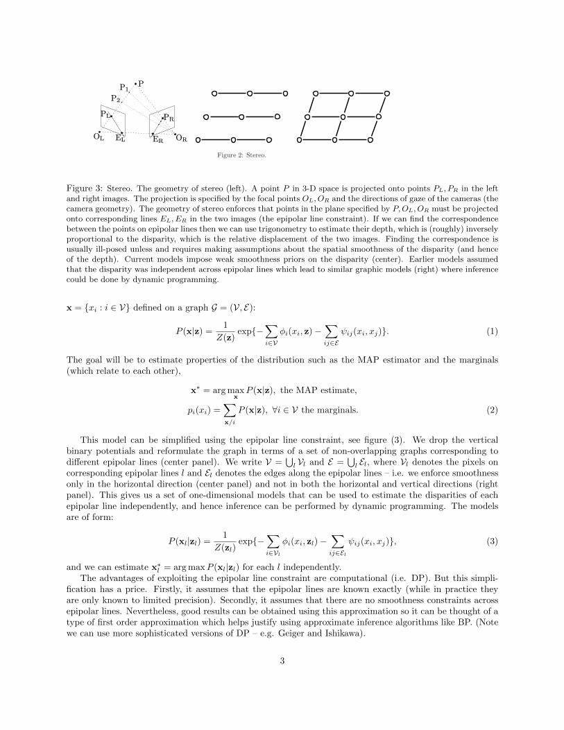
Figure 2: Stereo.

Figure 3: Stereo. The geometry of stereo (left). A point P in 3-D space is projected onto points PL, PR in the leftand right images. The projection is specified by the focal points OL, OR and the directions of gaze of the cameras (thecamera geometry). The geometry of stereo enforces that points in the plane specified by P,OL, OR must be projectedonto corresponding lines EL, ER in the two images (the epipolar line constraint). If we can find the correspondencebetween the points on epipolar lines then we can use trigonometry to estimate their depth, which is (roughly) inverselyproportional to the disparity, which is the relative displacement of the two images. Finding the correspondence isusually ill-posed unless and requires making assumptions about the spatial smoothness of the disparity (and henceof the depth). Current models impose weak smoothness priors on the disparity (center). Earlier models assumedthat the disparity was independent across epipolar lines which lead to similar graphic models (right) where inferencecould be done by dynamic programming.

x = {xi : i ∈ V} defined on a graph G = (V, E):

P (x|z) =1

Z(z)exp{−

∑i∈V

φi(xi, z)−∑ij∈E

ψij(xi, xj)}. (1)

The goal will be to estimate properties of the distribution such as the MAP estimator and the marginals(which relate to each other),

x∗ = arg maxx

P (x|z), the MAP estimate,

pi(xi) =∑x/i

P (x|z), ∀i ∈ V the marginals. (2)

This model can be simplified using the epipolar line constraint, see figure (3). We drop the verticalbinary potentials and reformulate the graph in terms of a set of non-overlapping graphs corresponding todifferent epipolar lines (center panel). We write V =

⋃l Vl and E =

⋃l El, where Vl denotes the pixels on

corresponding epipolar lines l and El denotes the edges along the epipolar lines – i.e. we enforce smoothnessonly in the horizontal direction (center panel) and not in both the horizontal and vertical directions (rightpanel). This gives us a set of one-dimensional models that can be used to estimate the disparities of eachepipolar line independently, and hence inference can be performed by dynamic programming. The modelsare of form:

P (xl|zl) =1

Z(zl)exp{−

∑i∈Vl

φi(xi, zl)−∑ij∈El

ψij(xi, xj)}, (3)

and we can estimate x∗l = arg maxP (xl|zl) for each l independently.The advantages of exploiting the epipolar line constraint are computational (i.e. DP). But this simpli-

fication has a price. Firstly, it assumes that the epipolar lines are known exactly (while in practice theyare only known to limited precision). Secondly, it assumes that there are no smoothness constraints acrossepipolar lines. Nevertheless, good results can be obtained using this approximation so it can be thought of atype of first order approximation which helps justify using approximate inference algorithms like BP. (Notewe can use more sophisticated versions of DP – e.g. Geiger and Ishikawa).

3

3 Belief Propagation

We now present a different approach to estimating (approximate) marginals and MAPs of an MRF. Thisis called belief propagation BP. It was originally proposed as a method for doing inference on trees (e.g.graphs without closed loops) [15] for which it is guaranteed to converge to the correct solution (and isrelated to dynamic programming). But empirical studies showed that belief propagation will often yieldgood approximate results on graphs which do have closed loops [14].

To illustrate the advantages of belief propagation, consider the binocular stereo problem which can beaddressed by using the first type of model. For binocular stereo there is the epipolar line constraint whichmeans that, provided we know the camera geometry, we can reduce the problem to one-dimensional matching,see figure (3). We impose weak smoothness in this dimension only and then use dynamic programming tosolve the problem [9]. But a better approach is to impose weak smoothness in both directions which can besolved (approximately) using belief propagation [18], see figure (3).

Surprisingly the fixed points of belief propagation algorithms correspond to the extreme of the Bethefree energy [20]. This free energy, see equation (9), appears better than the mean field theory free energybecause it includes pairwise pseudo-marginal distributions and reduces to the MFT free energy if these arereplaced by the product of unary marginals. But, except for graphs without closed loops (or a single closedloop), there are no theoretical results showing that the Bethe free energy yields a better approximation thanmean field theory. There is also no guarantee that BP will converge for general graphs and it can oscillatewidely.

3.1 Message Passing

BP is defined in terms of messages mij(xj) from i to j, and is specified by the sum-product update rule:

mt+1ij (xj) =

∑xi

exp{−ψij(xi, xj)− φi(xi)}∏k 6=j

mtki(xi). (4)

The unary and binary pseudomarginals are related to the messages by:

bti(xi) ∝ exp{−φi(xi)}∏k

mtkj(xj), (5)

btkj(xk, xj) ∝ exp{−ψkj(xk, xj)− φk(xk)− φj(xj)}

×∏τ 6=j

mtτk(xk)

∏l 6=k

mtlj(xj). (6)

The update rule for BP is not guaranteed to converge to a fixed point for general graphs and cansometimes oscillate wildly. It can be partially stabilized by adding a damping term to equation (4). Forexample, by multiplying the right hand side by (1− ε) and adding a term εmt

ij(xj).To understand the converge of BP observe that the pseudo-marginals b satisfy the admissibility constraint :∏

ij bij(xi, xj)∏i bi(xi)

ni−1∝ exp{−

∑ij

ψij(xi, xj)−∑i

φ(xi)} ∝ P (x), (7)

where ni is the number of edges that connect to node i. This means that the algorithm re-parameterizesthe distribution from an initial specification in terms of the φ, ψ to one in terms of the pseudo-marginalsb. For a tree, this re-parameterization is exact (i.e. the pseudo-marginals become the true marginals of

the distribution – e.g., we can represent a one-dimensional distribution by P (x) = 1Z {−

∑N−1i=1 ψ(xi, xi+1)−∑N

i=1 φi(xi)} or by∏N−1i=1 p(xi, xi+1)/

∏N−1i=2 p(xi).

It follows from the message updating equations (4,6) that at convergence, the b’s satisfy the consistencyconstraints:

4

Figure 5: Belief propagation

Figure 4: Message passing (left) is guaranteed to converge to the correct solution on graphs without closed loops(center) but only gives good approximations on graphs with a limited number of closed loops (right).

∑xj

bij(xi, xj) = bi(xi),∑xi

bij(xi, xj) = bj(xj). (8)

This follows from the fixed point conditions on the messages –mkj(xj) =∑xk

exp{−φk(xk)} exp{−ψjk(xj , xk)}∏l 6=jmlk(xk) ∀k, j, xj .In general, the admissibility and consistency constraints characterize the fixed points of belief propagation.

This has an elegant interpretation within the framework of information geometry [11].

3.2 Examples

BP is like dynamic programming for graphs without closed loops. The sum-product and max-product relateto the sum and max versions of dynamic programming (see earlier lecture). But there are several differences.Dynamic programming has forward and backward passes which do different operations (i.e. the pass differenttypes of messages). But BP only passes the same type of message. DP must start at either end of the graph,but BP can start anywhere and can proceed in parallel, see figure (5).

3.3 The Bethe Free Energy

The Bethe free energy [7] differs from the MFT free energy by including pairwise pseudo-marginals bij(xi, xj):

F [b;λ] =∑ij

∑xi,xj

bij(xi, xj)ψij(xi, xj) +∑i

∑xi

bi(xi)φi(xi)

+∑ij

∑xi,xj

bij(xi, xj) log bij(xi, xj)−∑i

(ni − 1)∑xi

bi(xi) log bi(xi), (9)

But we must also impose consistency and normalization constraints which we impose by lagrange multi-pliers {λij(xj)} and {γi}:

∑i,j

∑xj

λij(xj){∑xi

bij(xi, xj)− bj(xj)}

+∑i,j

∑xi

λji(xi){∑xj

bij(xi, xj)− bi(xi)}+∑i

γi{∑xi

bi(xi)− 1}. (10)

5

Figure 5: Example of message passing for a graph without closed loops. The messages can start at any node and canbe updated in parallel. But the most efficient way is to start messages from the boundaries (because these messagesare fixed and will not need to be updated, which causes the algorithm to converge faster.

It is straightforward to verify that the extreme of the Bethe free energy also obey the admissibility andconsistency constraints – set the derivatives of the Bethe free energy to zero. Hence the fixed points of beliefpropagation correspond to extrema of the Bethe free energy.

3.4 Where do the messages come from? The dual formulation.

Where do the messages in belief propagation come from? At first glance, they do not appear directly inthe Bethe free energy (Pearl has motivation for performing inference on graphs without closed loops). Butobserve that the consistency constraints are imposed by lagrange multipliers λij(xj) which have the samedimensions as the messages.

We can think of the Bethe free energy as specifying a primal problem defined over primal variables b anddual variables λ. The goal is to minimize F [b;λ] with respect to the primal variables and maximize it withrespect to the dual variables. There corresponds a dual problem which can be obtained by minimizing F [b;λ]with respect to b to get solutions b(λ) and substituting them back to obtain F̂d[λ] = F [b(λ);λ]. Extrema ofthe dual problem correspond to extrema of the primal problem (and vice versa). Note: but there is a dualitygap because the Bethe free energy is not convex except for graphs without closed loops. This means thatthe relationship between the solution of the primal and dual problems are complicated (revise this).

It is straightforward to show that minimizing F with respect to the b’s give the equations:

bti(xi) ∝ exp{−1/(ni − 1){γi −∑j

λji(xi)− φi(xi)}}, (11)

btij(xi, xj) ∝ exp{−ψij(xi, xj)− λtij(xj)− λtji(xi)}. (12)

6

Observe the similarity between these equations and those specified by belief propagation, see equa-tions (4). They become identical if we identify the messages with a function of the λ’s:

λji(xi) = −∑

k∈N(i)/j

logmki(xi). (13)

There are, however, two limitations of the Bethe free energy. Firstly it does not provide a bound ofthe partition function (unlike MFT) and so it is not possible to using bounding arguments to claim thatBethe is ’better’ than MFT (i.e. it is not guaranteed to give a tighter bound). Secondly, Bethe is non-convex(except on trees) which has unfortunate consequences for the dual problem – the maximum of the dual is notguaranteed to correspond to the minimum of the primal. Both problems can be avoided by an alternativeapproach, described in the next section, which gives convex upper bounds on the partition function andspecifies convergent (single-loop) algorithms.

3.5 Extras about Belief Propagation

If the goal of belief propagation is to minimize the Bethe Free Energy then why not use direct methods likesteepest descent or discrete iterative algorithms instead? One disadvantage is these methods require workingwith pseudomarginals that have higher dimensions than the messages (contrast bij(xi, xj) with mij(xj)).Discrete iterative algorithms have been proposed [21],[10] which are more stable than belief propagation andwhich can reach lower values of the Bethe Free Energy. But these DIA must have an inner loop to dealwith the consistency constraints and hence take longer to converge than belief propagation. The differencebetween these direct algorithms and belief propagation can also be given an elegant geometric interpretationin terms of information geometry [11].

Belief propagation can also be formulated as re-parametrizing the probability distribution (Wainwright).This following from the admissibility constraint. We start off by expressing the probability distribution interms of potentials (i.e. the way we formulate an undirected graphical model) and the output of BP – theunary and binary marginals – allow us to reformulate the probability distribution in terms of approximateconditional distributions. If the graph has no closed loops, then it is possible to express the probabilitydistribution exactly in terms of conditional distributions – and DP (the sum version) will also enable us todo this ”translation”. This gives rise to an alternative formulation of BP which does not use messages, seefigure (6).

Figure 6: BP without messages. Use current estimates of unary and binary beliefs to define distributions over groupsof nodes (left panel). Then re-estimate the unary and binary beliefs by marginalization (right panel).

There is also a relationship between BP and a form of Gibbs sampling [16] which follows from theformulation of BP without messages, see figure (6). In a sense, BP is like taking the expectation of the updateprovided by a Gibbs sampling algorithm that samples pairs of points at the same time. The relationshipbetween sampling techniques and deterministic methods is an interesting area of research and there aresuccessful algorithms which combine both aspects. For example, there are recent nonparametric approacheswhich combine particle filters with belief propagation to do inference on graphical models where the variablesare continuous valued [17][12].

7

Work by Felzenszwalb and Huttenlocher [8] shows how belief propagation methods can be made extremelyfast by taking advantage of properties of the potentials and the multi-scale properties of many vision prob-lems. Researchers in the UAI community have discovered ways to derive generalizations of BP starting fromthe perspective of efficient exact inference [6].

4 Generalized Belief Propagation and the Kikuchi Free Energy

Not covered in class. It shows that BP can be generalized naturally to graphs where there are higher orderinteractions.

The Bethe free energy and belief propagation were defined for probability distributions defined overgraphs with pairwise interactions (e.g. potential terms like ψij(xi, xj)). If we have higher order interactionsthen we can generalize to the Kikuchi free energy and generalized belief propagation [7][20]

Let R be the set of regions that contain basic clusters of nodes, their intersections, the intersections oftheir intersections, and so on. For any region r, we define the super-regions of r to be the set sup(r) of all ofregions in R that contain r. The sub-regions of r are the set sub(r) of all regions of in R that lie completelywithin r. The direct sub-regions of r are the set subd(r) of all sub-regions of r which have no super-regionswhich are also sub-regions of r. The direct super-regions supd(r) are the super-regions of r that have nosub-regions which are also super-regions of r.

Let xr be the state of nodes in region r and br(xr) is the belief. Er(xr) is the energy associated with theregion (e.g. −

∑(i,j)∈R ψij(xi, xj)−

∑i∈r ψi(xi)). The Kikuchi Free energy is:

FK =∑r∈R

cr{∑xr

br(xr)Er(xr)}+∑xr

br(xr) log br(xr) + Lk. (14)

cr is an over-counting number defined by cr = 1−∑s∈sup(r) cs. Lk imposes the constraints.

∑r γr{

∑xrbr(xr)−

1}+∑r

∑s∈subd(r)λr,s(xs){

∑x∈r/s

br(xr)− bs(xs)}, where r/s is the complement of s in r.

As before, there is a dual formulation of Kikuchi in terms of dual variables which motivates a generalizedbelief propagation (GBP) algorithm in terms of the dual variables which can be converted into messages.Double loop algorithms such as CCCP can also be directly applied to Kikuchi [?]. In short, all the propertiesof Bethe and belief propagation can be extended to this case.

For example, minimizing Kikuchi with respect to the beliefs b gives solutions in terms of messages:

br(xr) = ψr(xr)∏

(u,v)∈M(r)

muv(xv). (15)

Generalized belief propagation can be defined by message updating:

mrs(xs : t+ 1) = mrs(xs : t)

∑x∈r/s exp{−ψr(xr)}

∏(u,v)∈M(r)muv(xv)

exp{−ψs(xs)}∏

(u,v)∈M(s)muv(xv). (16)

5 Convex Upper Bounds and TRW

Not covered in class. Advanced material. Bottom line - people should probably use TRW instead of BP.TRW is an alternative to the BP algorithm. It is theoretical much cleaner than BP and it yields better

performance in practice (although how much to trust those types of comparisons – the improvements arenot enormous). Instead of the Bethe free energy it starts with a convex free energy which is specified as anupper bound of the log partition function of the distribution (recall that Bethe is not a bound). This freeenergy becomes identical to the Bethe free energy for graphs without closed loops. There is also no dualitygap between the free energy and its dual. Hence there are algorithms in dual space (similar to BP) whichare guaranteed to converge to the global optimum (give some caveats!).

This section specifies an alternative class of convex free energies which are defined to be upper boundsof the log partition function. They lead to free energies which are similar to Bethe and to algorithms which

8

are similar to belief propagation. But they have several advantages. Firstly, they gives bounds so it is moreeasy to quantify how good they are as approximations. Secondly, they are convex so algorithms exist whichcan find their global minimum. Thirdly, they enable algorithms similar to belief propagation which areguaranteed to converge.

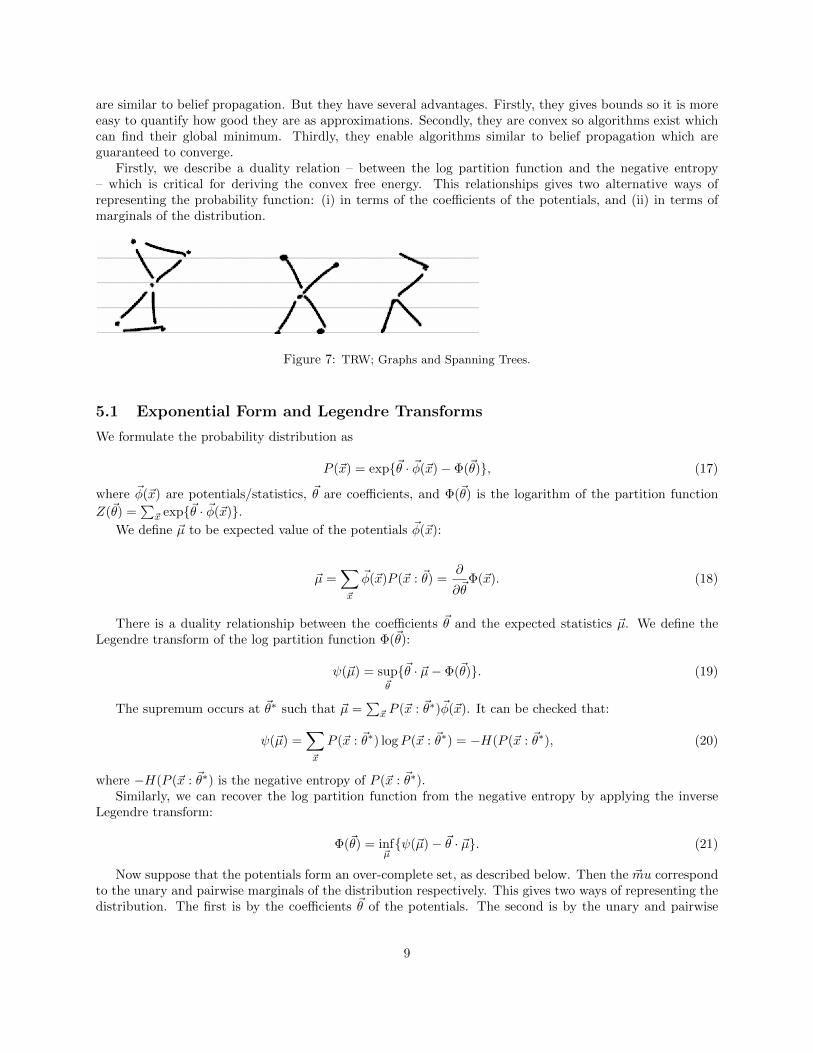
Firstly, we describe a duality relation – between the log partition function and the negative entropy– which is critical for deriving the convex free energy. This relationships gives two alternative ways ofrepresenting the probability function: (i) in terms of the coefficients of the potentials, and (ii) in terms ofmarginals of the distribution.

Figure 7: TRW; Graphs and Spanning Trees.

5.1 Exponential Form and Legendre Transforms

We formulate the probability distribution as

P (~x) = exp{~θ · ~φ(~x)− Φ(~θ)}, (17)

where ~φ(~x) are potentials/statistics, ~θ are coefficients, and Φ(~θ) is the logarithm of the partition function

Z(~θ) =∑~x exp{~θ · ~φ(~x)}.

We define ~µ to be expected value of the potentials ~φ(~x):

~µ =∑~x

~φ(~x)P (~x : ~θ) =∂

∂~θΦ(~x). (18)

There is a duality relationship between the coefficients ~θ and the expected statistics ~µ. We define theLegendre transform of the log partition function Φ(~θ):

ψ(~µ) = sup~θ

{~θ · ~µ− Φ(~θ)}. (19)

The supremum occurs at ~θ∗ such that ~µ =∑~x P (~x : ~θ∗)~φ(~x). It can be checked that:

ψ(~µ) =∑~x

P (~x : ~θ∗) logP (~x : ~θ∗) = −H(P (~x : ~θ∗), (20)

where −H(P (~x : ~θ∗) is the negative entropy of P (~x : ~θ∗).Similarly, we can recover the log partition function from the negative entropy by applying the inverse

Legendre transform:

Φ(~θ) = inf~µ{ψ(~µ)− ~θ · ~µ}. (21)

Now suppose that the potentials form an over-complete set, as described below. Then the ~mu correspondto the unary and pairwise marginals of the distribution respectively. This gives two ways of representing thedistribution. The first is by the coefficients ~θ of the potentials. The second is by the unary and pairwise

9

marginals. As described earlier (where??), if the distributions are defined over a graph with no loops (i.e. atree) then it is easy to translate from one representation to the other. This relationship will be exploited aswe derive the convex free energy.

5.2 Obtaining the Upper Bound

The strategy to obtain the convex free is based on exploiting the fact that everything is easy on graphswith no loops (i.e. trees). So the strategy is to define a probability distribution ρ(T ) on the set of spanning

trees T of the graph – i.e. ρ(T ) ≥ 0 and∑T ρ(T ) = 1. For each tree, we define parameters ~θ(T ) with the

constraint that∑T ρ(T )~θ(T ) = ~θ. On each spanning tree we are able to compute the entropy and partition

function of the distribution defined on the tree. We now show how this can be exploited to provide an upperbound on the partition function for the full distribution.

We first bound the partition function by the averaged sum of the partition functions on the spanningtrees (using Jensen’s inequality):

Φ(~θ) = Φ(∑T

ρ(T )~θ(T )) ≤∑T

ρ(T )Φ(~θ(T )). (22)

We can make the bound tighter by solving the constrained minimization problem:∑T

ρ(T )Φ(~θ(T ))− ~τ · {∑T

ρ(T )~θ(T )− ~θ}. (23)

Here the ~τ are Lagrange multipliers. In more detail, we define a set of over-complete potentials {φs(xs; k), φst(xs, xt; k, l)}where s ∈ V (s, t) ∈ E are the nodes and edges of the graph, xs are the state variables, and k, l index thevalues that the state variables can take. We define corresponding parameters {θs(k;T ), θst(k, l : T )}. Thenthe ~τ can be written as {τs(k), τst(k, l)}.

Minimizing equation (23) with respect to ~θ(T ) gives the equations:

ρ(T )∑~x

~θ∗(T )P (~x : ~θ∗(T )) = ρ(T )~τ . (24)

Recall that each spanning tree T will contain all the nodes V but only a subset E(T ) of the edges.

Equation (24) determines that we can express P (~x : ~θ∗(T )) in terms of the dual variables {τs : s ∈ V }, {τst :(s, t) ∈ E(T )}:

P (~x : ~θ∗(T )) =∏s

τs(xs)∏

(s,t)∈E(T )

τst(xs, xt)

τs(xs)τt(xt). (25)

Equation (25) is very insightful. It tells us that the ~τ , which started out as Lagrange multipliers, canbe interpreted (at the extremum) as pseudo-marginals obeying the consistency constraints

∑xsτs(xs) = 1,∑

xtτst(xs, xt) = τs(xs), and so on. It tells us that the ~θ(T ) are related to the same ~τ for all T , although for

each T some of the ~τ terms will not be used (those corresponding to the missing edges in T ). It also tells

us that we can evaluate the terms Φ(~θ∗) involved in the bound – they can be computed from the Legendre

transform (ref backwards!!) in terms of ~τ · ~θ∗(T ) and the negative entropy of P (~x : ~θ∗(T )), which can beeasily computed from equation (25) to be:

~τ · ~θ∗(T ) = ~θ∗(T ) · ~τ +∑s

Hs +∑

(s,t)∈E(T )

Ist. (26)

We compute the full bound by taking the expectation with respect to ρ(T ) (using the constraint∑T ρ(T )~θ∗(T ) =

~θ) yielding the free energy:

10

Fconbound = −~θ · ~τ +∑s

Hs +∑

(s,t)∈E

ρstIst. (27)

Next we use the inverse Legendre transform to express the right hand side of equation (22) as a freeenergy which, by the derivation, is convex in terms of the pseudomarginals µ:

F(µ : ρ, θ) = −∑s

Hs(µs) +∑

(s,t)∈E

TstIst(µst)− ~µ · ~θ, (28)

where Hs(Ts) = −∑j Ts:j log Ts:j and Ist(Tst) =

∑ij Tst:jk log

Tst:jk(∑k Tst;jk)(

∑j Tst:jkθ

∗st;jk) . This is the expec-

tation with respect to the distribution ρ(T ) over trees of the entropies defined on the trees. The pseudo-marginals must satisfy the consistency constraints which are imposed by lagrange multipliers.

5.3 TRW algorithm

The bound on the partition function can be obtained by minimizing the free energy F(µ : ρθ) with respect toµ, and the resulting pseudomarginals µ can be used as estimators of the marginals of P (~x). By minimizing thefree energy with respect to µ we can express the pseudmarginals as messages (similar to Bethe): (REMOVETHE ∗’s!!):

µs(xt) = k exp{φs(xs : θ∗s)}∏

ν∈Γ(s)

|Mνs(xs)|µνs ,

µst(xs, xt) = Kφst(xs, xt : θ∗)

∏ν∈Γ(s)/t |Mνs(xs)|µνs

|Mts(xs)|1−µst

×∏ν∈Γ(t)/s |Mνt(xt)|µνt

|Mst(xt)|1−µts, (29)

where the quantity φs(xs; θ∗s) takes value θ∗st when xs = j and analogously for φst(xs, xt : θ∗st).

It can be checked that these pseudomarginals satisfy the admissability conditions:

θ∗ · φ(x) + C =∑ν∈V

log µ̂(xs) +∑

(s, t) ∈ Eρst logµ̂st(xs, xt)

T̂s(xs)T̂t(xt). (30)

The TRW algorithm updates the messages by the following rules. The fixed points occur at the globalminimum of the free energy, but there is no guarantee that the algorithm will converge.

Initialize the messages M0 = {Mst} with arbitrary positive values. For iterations n = 0, 1, .... update themessages by:

Mn+1ts (xs) = K

∑x′t∈Xt

exp{ 1

µstφst(xs, x

′t; θ∗st) + φt(x

′t : θ∗t )}

{∏ν∈Γ(t)/s{Mn

νi(x′t)}µνt

|Mnst(x

′t)|(1−µts)

}. (31)

11

5.4 A convergent variant

An alternative approach by Globerson and Jaakkola uses the same strategy to obtain a free energy function.They write a slightly different free energy:

−µ · θ −∑i

ρ0iH(Xi)−∑ij∈E

ρi|jH(Xi|Xj), (32)

which agrees with the TRW free energy if the pseudomarginals µ satisfy the constraints but differs elsewhere.The advantage is that they can explicitly computer the dual of the free energy. This dual free energy isexpressed as: ∑

i

ρ0i log∑xi

exp{ρ−1j|i {θij(xi, xj)−

∑k∈N(i)

λk|i(i: β)}}. (33)

where

λj|i(xi : β) = −ρj|i log∑xj

exp{ρ−1j|i {θij(xi, xj) + δj|iβij(xi, xj)}}. (34)

The β variables are dual variables.The explicit form of the dual (not known for the TRW free energy) makes it possible to derive an iterative

algorithm that is guaranteed to converge. The update rule is specified by:

βt+1ij (xi, xj) = βtij(xi, xj) + ε log

µtj|i(xj |xi)µti(xi)

µti|j(xi|xj)µtj(xj)

. (35)

It can be checked that this update satisfies the tree re-parameterization conditions.Note: CCCP will give a provably convergent algorithm but relies on a double loop (Nishihara et al).

6 Conclusions

This lecture described MRF methods for addressing the stereo correspondence problem and discussed howthey could be solved using dynamic programming – exploiting the epipolar line constraint – or by beliefpropagation if we allow interactions across the epipolar lines.

We also introduced belief propagation and also the TRW algorithm (not covered in class).

References

[1] Y. Amit. “Modelling Brain Function: The World of Attrcator Neural Networks”. Cambridge UniversityPress. 1992.

[2] C.M. Bishop. Pattern Recognition and Machine Learning. Springer. Second edition. 2007.

[3] M. J. Black and A. Rangarajan, ”On the unification of line process, outlier rejection, and robust statisticswith applications in early vision”, Int’l J. of Comp. Vis., Vol. 19, No. 1 pp 57-91. 1996.

[4] S. Roth and M. Black. Fields of Experts. International Journal of Computer Vision. Vol. 82. Issue 2. pp205-229. 2009.

[5] A. Blake, and M. Isard: The CONDENSATION Algorithm - Conditional Density Propagation andApplications to Visual Tracking. NIPS 1996: 361-367. 1996.

12

[6] A. Choi and A. Darwiche. A Variational Approach for Approximating Bayesian Networks by EdgeDeletion. In Proceedings of the 22nd Conference on Uncertainty in Artificial Intelligence (UAI), pages80-89, 2006.

[7] C. Domb and M.S. Green. Eds. Phase Transitions and Critical Phenomena. Vol.2. Academic Press.London. 1972.

[8] P. Felzenszwalb and D. P. Huttenlocher. Efficient Belief Propagation for Early Vision. Proceedings ofComputer Vision and Pattern Recognition. 2004.

[9] D. Geiger, B. Ladendorf and A.L. Yuille. “Occlusions and binocular stereo”.International Journal ofComputer Vision. 14, pp 211-226. 1995.

[10] T. Heskes, K. Albers and B. Kappen. Approximate Inference and Constrained Optimization. Proc. 19thConference. Uncertainty in Artificial Intelligence. 2003.

[11] S. Ikeda, T. Tanaka, S. Amari. “Stochastic Reasoning, Free Energy, and Information Geometry”. NeuralComputation. 2004.

[12] M. Isard, ”PAMPAS: Real-Valued Graphical Models for Computer Vision,” cvpr, vol. 1, pp.613, 2003IEEE Computer Society Conference on Computer Vision and Pattern Recognition (CVPR ’03) - Volume1, 2003.

[13] J. Lafferty, A. McCallum, and F. Pereira. Conditional random fields: Probabilistic models for segmentingand labeling sequence data. In: Proc. 18th International Conf. on Machine Learning, Morgan Kaufmann,San Francisco, CA. 2001.

[14] R.J. McEliece, D.J.C. MacKay, and J.F. Cheng. Turbo Decoding as an instance of Pearl’s belief prop-agation algorithm. IEEE Journal on Selected Areas in Communication. 16(2), pp 140-152. 1998.

[15] J. Pearl. “Probabilistic Reasoning in Intelligent Systems: Networks of Plausible Inference.” MorganKaufmann, San Mateo, CA. 1988.

[16] M. Rosen-Zvi, M. I. Jordan, A. L. Yuille: The DLR Hierarchy of Approximate Inference. Uncertaintyin Artificial Intelligence. 2005: 493-500.

[17] E. Sudderth, A.T. Ihler, W.T. Freeman, and A.S. Willsky. Nonparametric Belief Propagation. CVPR.pp 605-612. 2002.

[18] J. Sun, H-Y Shum, and N-N Zheng. Stereo Matching using Belief Propagation. Proc. 7th EuropeanConference on Computer Vision. pp 510-524. 2005.

[19] M.J. Wainwright, T.S. Jaakkola, and A.S. Willsky. “Tree-Based Reparamterization Framework for Anal-ysis of Sum-Product and Related Algorithms”. IEEE Transactions on Information Theory. Vol. 49, pp1120-1146. No. 5. 2003.

[20] J.S. Yedidia, W.T. Freeman, and Y. Weiss, “Generalized belief propagation”. In Advances in NeuralInformation Processing Systems 13, pp 689-695. 2001.

[21] A.L. Yuille. “CCCP Algorithms to Minimize the Bethe and Kikuchi Free Energies: Convergent Alter-natives to Belief Propagation”. Neural Computation. Vol. 14. No. 7. pp 1691-1722. 2002.

[22] A.L. Yuille and Anand Rangarajan. “The Concave-Convex Procedure (CCCP)”. Neural Computation.15:915-936. 2003.

13