
© 2006 by Davi GeigerComputer Vision April 2006 L1.1 Binocular Stereo Left Image Right Image.
14
Computer Vision April 2006 L1.1 © 2006 by Davi Geiger Binocular Stereo Binocular Stereo Left Image Right Image
-
date post
21-Dec-2015 -
Category
Documents
-
view
213 -
download
0
Transcript of © 2006 by Davi GeigerComputer Vision April 2006 L1.1 Binocular Stereo Left Image Right Image.

Computer Vision April 2006 L1.1© 2006 by Davi Geiger
Binocular Stereo
Binocular Stereo
Left Image Right Image

Computer Vision April 2006 L1.2© 2006 by Davi Geiger
Each potential match is represented by a square. The black ones represent the most likely scene to “explain” the image, but other combinations could have given rise to the same image (e.g., red)
Stereo Correspondence: Ambiguities
What makes the set of black squares preferred/unique is that they have similar disparity values, the ordering constraint is satisfied and there is a unique match for each point. Any other set that could have given rise to the two images would have disparity values varying more, and either the ordering constraint violated or the uniqueness violated. The disparity values are inversely proportional to the depth values

Computer Vision April 2006 L1.3© 2006 by Davi Geiger
A BC
DE F
AB
A
CD
DC
F
FE
Stereo Correspondence: Matching Space
Rig
ht
boundary
no m
atc
hBoundary no match
Left
depth discontinuity
Surface orientation
discontinuity
F D C B A
AC
D
E
F
Note 2: Due to pixel discretization, points A and C in the right frame are neighbors.
Note 1: Depth discontinuities and very tilted surfaces can/will yield the same images ( with half occluded pixels)
In the matching space, a point (or a node) represents a match of a pixel in the left image with a pixel in the right image

Computer Vision April 2006 L1.4© 2006 by Davi Geiger
Cyclopean Eye
2and
22 and
2
wxl
wxr
lrw
lrx
w
x
l
r
l
r
w
x
11
11
2
1
11
11
2
1
The cyclopean eye “sees” the world in 3D where x represents the coordinate system of this eye and w is the disparity axis
For manipulating with integer coordinate values, one can also use the following representation
w
x
l
r
l
r
w
x
11
11
2
1
11
11
Restricted to integer values. Thus, for l,r=0,…,N-1 we have x=0,…2N-2 and w=-N+1, .., 0, …, N-1
Note: Not every pair (x,w) have a correspondence to (l,r), when only integer coordinates are considered. Indeed, the integer coordinate system (x,w) exhibit subpixel accuracy.For x+w even we have integer values for pixels r and l and for x+w odd we have supixel locations.
ooooooo
ooooooo
ooooooo
ooooooo
ooooooo
ooooooo
ooooooo
w
w=2
Right Epipolar Line
l-1 l=3 l+1
r+1
r=5
r-1
x

Computer Vision April 2006 L1.5© 2006 by Davi Geiger
Surface ConstraintsSmoothness : In nature most surfaces are smooth in depth compared to their distance to the observer, but depth discontinuities also occur. Usually smoothness implies an ordering constraint, where points to the right of match point to the right of
Uniqueness: There should be only one disparity value associated to each cyclopean coordinate x. Note, multiple matches for left eye points or right eye points are allowed.
lq
rq
Left Epipolar Line
w
ooooo
ooooo
ooooooo
oooooo
oooooo
oooooo
ooooooo
w=2
Left Epipolar Line
Right Epipolar Line
w=3
w=0
w=-2
Uniqueness
l-1 l=3 l+1
r+1
r=5
r-1
x
x=8
ooooooo
ooooooo
ooooooo
ooooooo
oooooo
ooooooo
ooooooo
w
w=2
Right Epipolar LineSmoothness (+Ordering)
l-1 l=3 l+1
r+1
r=5
r-1
x
x=8

Computer Vision April 2006 L1.6© 2006 by Davi Geiger
Bayesian Formulation
)}),(),,(({
))},(({)}),({|)},(),,(({)}),(),,(|),(({
eqIeqIP
exwPexweqIeqIPeqIeqIexwP
rR
lL
rR
lL
rR
lL
The probability of a surface w(x,e) to account for the left and right image can be described by the Bayes formula as
Let us develop formulas for both probability terms on the numerator. The denominator is a normalization to make the probability sum to 1.

Computer Vision April 2006 L1.7© 2006 by Davi Geiger
C(e,x,w) Є [0,1], x+w even, represents how good is a match between a point (e,l) in the left image and a point (e,r) in the right image (where x=l+r is the cyclopean eye coordinate and w=r-l is the disparity.) The epipolar lines are indexed by e (for the homework, they are just the horizontal lines).
C(e,x,w) Є [0,1], x+w odd, represents how good is a match between an edge (e,l -> l+1) in the left image and an edge (e,r ->r+1) in the right image
1
0
22
0
),,(1)}),({|)},(),,(({
N
e
N
x
wxeC
rR
lL e
ZexweqIeqIP
2r ,
2 odd
),0,(),0,(
),0,(),0,(
even255
),(),(
),,(wxwx
lwxerDIelDI
erDIelDI
wxerIelI
wxeC
RL
RL
RL
The parameter reduces the effect of the gradient values.

Computer Vision April 2006 L1.8© 2006 by Davi Geiger
even)),1(),,(( wxforexwexwF
w
w=2
Right Epipolar Line
l-1 l=3 l+1
r+1
r=5
r-1
x
x=80)),1(),,((
),1(),( if
_)),1(),,((
1),1(),(1),1(),( if
exwexwF
exwexw
CostTILTexwexwF
exwexworexwexw
1)5,2
,()5,2
,()),),,((
rDIlDIexexwD
RL
Epipolar interaction: the higher the intensity edges the less the cost (the higher the probability) to have disparity changes across epipolar lines
1),1(),( where
1),(
1
0
22
0
2)1,(),(),),,(()),1(),,((
exwexw
eZ
exwP
N
e
N
x
exwexwexexwDexwexwF

Computer Vision April 2006 L1.9© 2006 by Davi Geiger
1),1(),( where
1),(
1
0
22
0
2)1,(),(),),,(()),1(),,((
exwexw
eZ
exwP
N
e
N
x
exwexwexexwDexwexwF
w
w=2
Right Epipolar Line
l-1 l=3 l+1
r+1
r=5
r-1
x
x=8
0)),1(),,((
),1(),( if
1)5,0,(
_)),1(),,((
)(1),1(),( if
1)5,0,(
_)),1(),,((
)(1),1(),( if
exwexwF
subpixeltopixelexwexw
rDI
CostOcclusionexwexwF
occlusionsubpixeltosubpixelexwexw
lDI
CostOcclusionexwexwF
occlusionsubpixeltosubpixelexwexw
R
L
odd)),1(),,(( wxforexwexwF

Computer Vision April 2006 L1.10© 2006 by Davi Geiger
Limit Disparity
The matrix is updated only within a range of
disparity : 2D+1 , i.e.,
The rational is:
(i) Less computations
(ii) Larger disparity matches imply larger errors in 3D estimation.
Dlrw ||||
w=-3
w
w=2
Right Epipolar LineSmoothness (+Ordering)
l-1 l=3 l+1
r+1
r=5
r-1
x
x=8
D=3
Dw ||

Computer Vision April 2006 L1.11© 2006 by Davi Geiger
1),1(),( where
1),|)},(({
1
0
22
0
2)1,(),(),),,(()),1(),,((),),,((
exwexw
eZ
IIexwP
N
e
N
x
exwexwexexwDexwexwFexexwCRL
Stereo Correspondence: Belief Propagation (BP)
We want to obtain/compute the marginal
We have finally the posterior distribution for disparity values (surface {w(x,e)})
D
DNexw
D
DNexw
D
DNeNxw
RL
D
Dexw
D
Deexxw
D
DeNxw
D
Dexw
D
Dexw
D
DeNxw
D
Dexw
D
Dexw
D
Dexw
D
DeNxw
IIexwP
exexwP
)',0'( )','( ),22'(
)',0'( )'&'( )',22'(
)1,0'( )1','( )1',22'(
)0',0'( )0',1'( )0','( )0',22'(
),|)}','(({......
...
......
...
......
......),),,((
These are exponential computations on the size of the grid N

Computer Vision April 2006 L1.12© 2006 by Davi Geiger
12 w
x
e e
x
“Horizontal” Belief Tree
)),((h exwP )),((v exwP
“Vertical” Belief Tree
Kai Ju’s approximation to BP
12 w
We use Kai Ju’s Ph.D. thesis work to approximate the (x,e) graph/lattice by horizontal and vertical graphs, which are singly connected. Thus, exact computation of the marginal in these graphs can be obtained in linear time. We combine the probabilities obtained for the horizontal and vertical graphs, for each lattice site, by “picking” the “best” one (the ones with lower entropy, where .)
D
Dw
exwPexwPexS )),((log)),((),(
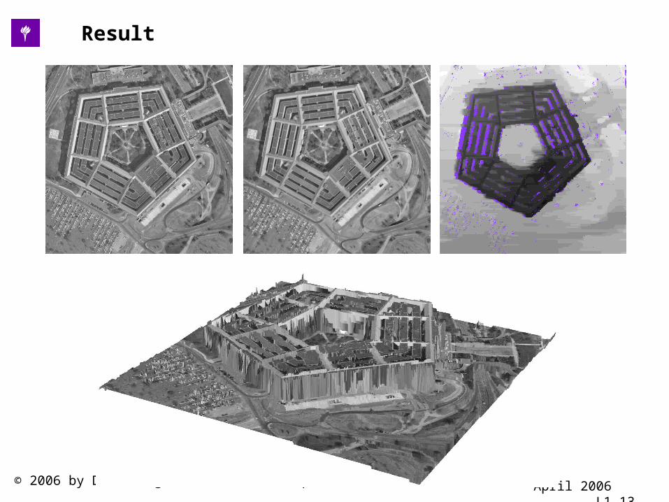
Computer Vision April 2006 L1.13© 2006 by Davi Geiger
Result

Computer Vision April 2006 L1.14© 2006 by Davi Geiger
Region A
Region B
Region A Left
Region A Right
Region B Left
Region B Right
Junctions and its properties (false matches that reveal information from vertical disparities (see Malik 94, ECCV)
Some Issues in Stereo: