Lect09
50
1 EEE 498/598 EEE 498/598 Overview of Electrical Overview of Electrical Engineering Engineering Lecture 9: Faraday’s Law Of Lecture 9: Faraday’s Law Of Electromagnetic Induction; Electromagnetic Induction; Displacement Current; Complex Displacement Current; Complex Permittivity and Permeability Permittivity and Permeability
-
Upload
abel-carrasquilla -
Category
Engineering
-
view
49 -
download
1
Transcript of Lect09

1
EEE 498/598EEE 498/598Overview of Electrical Overview of Electrical
EngineeringEngineering
Lecture 9: Faraday’s Law Of Lecture 9: Faraday’s Law Of Electromagnetic Induction; Electromagnetic Induction;
Displacement Current; Complex Displacement Current; Complex Permittivity and PermeabilityPermittivity and Permeability
2 Lecture 9
Lecture 9 ObjectivesLecture 9 Objectives
To study Faraday’s law of electromagnetic To study Faraday’s law of electromagnetic induction; displacement current; and induction; displacement current; and complex permittivity and permeability.complex permittivity and permeability.

3 Lecture 9
Fundamental Laws of Fundamental Laws of ElectrostaticsElectrostatics
Integral formIntegral form Differential formDifferential form
∫∫
∫=⋅
=⋅
V
ev
S
C
dvqsdD
ldE 0
evqD
E
=⋅∇=×∇ 0
ED ε=

4 Lecture 9
Fundamental Laws of Fundamental Laws of MagnetostaticsMagnetostatics
Integral formIntegral form Differential formDifferential form
0=⋅
⋅=⋅
∫
∫∫
S
SC
sdB
sdJldH
0=⋅∇=×∇
B
JH
HB µ=

5 Lecture 9
Electrostatic, Magnetostatic, and Electrostatic, Magnetostatic, and Electromagnetostatic FieldsElectromagnetostatic Fields
In the static case (no time variation), the electric In the static case (no time variation), the electric field (specified by field (specified by EE and and DD) and the magnetic ) and the magnetic field (specified by field (specified by BB and and HH) are described by ) are described by separate and independent sets of equations.separate and independent sets of equations.
In a conducting medium, both electrostatic and In a conducting medium, both electrostatic and magnetostatic fields can exist, and are coupled magnetostatic fields can exist, and are coupled through the Ohm’s law (through the Ohm’s law (JJ = = σσEE). Such a ). Such a situation is called situation is called electromagnetostaticelectromagnetostatic ..

6 Lecture 9
Electromagnetostatic FieldsElectromagnetostatic Fields
In an electromagnetostatic field, the electric field In an electromagnetostatic field, the electric field is completely determined by the stationary is completely determined by the stationary charges present in the system, and the magnetic charges present in the system, and the magnetic field is completely determined by the current.field is completely determined by the current.
The magnetic field does not enter into the The magnetic field does not enter into the calculation of the electric field, nor does the calculation of the electric field, nor does the electric field enter into the calculation of the electric field enter into the calculation of the magnetic field.magnetic field.

7 Lecture 9
The Three Experimental Pillars The Three Experimental Pillars of Electromagneticsof Electromagnetics
Electric charges attract/repel each other as Electric charges attract/repel each other as described by described by Coulomb’s lawCoulomb’s law..
Current-carrying wires attract/repel each other Current-carrying wires attract/repel each other as described by as described by Ampere’s law of forceAmpere’s law of force..
Magnetic fields that change with time induce Magnetic fields that change with time induce electromotive force as described by electromotive force as described by Faraday’s Faraday’s lawlaw..

8 Lecture 9
Faraday’s ExperimentFaraday’s Experiment
battery
switch
toroidal ironcore
compass
primarycoil
secondarycoil
9 Lecture 9
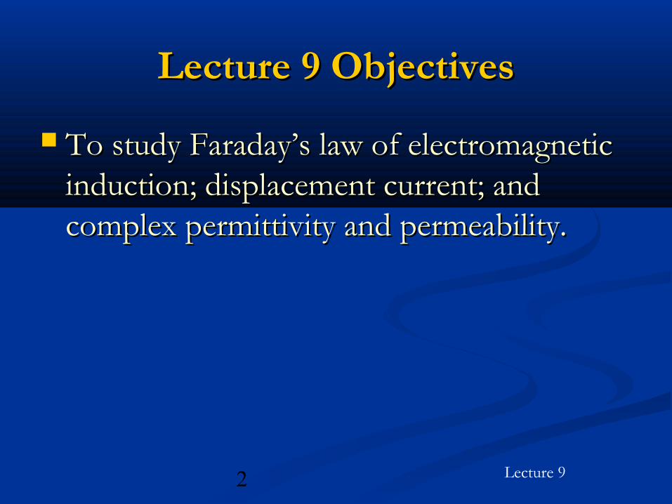
Faraday’s Experiment (Cont’d)Faraday’s Experiment (Cont’d)
Upon closing the switch, current begins to flow Upon closing the switch, current begins to flow in the in the primary coilprimary coil..
A momentary deflection of the A momentary deflection of the compasscompass needleneedle indicates a brief surge of current flowing in the indicates a brief surge of current flowing in the secondary coilsecondary coil..
The The compass needlecompass needle quickly settles back to quickly settles back to zero.zero.
Upon opening the switch, another brief Upon opening the switch, another brief deflection of the deflection of the compass needlecompass needle is observed. is observed.
10 Lecture 9
Faraday’s Law of Faraday’s Law of Electromagnetic InductionElectromagnetic Induction
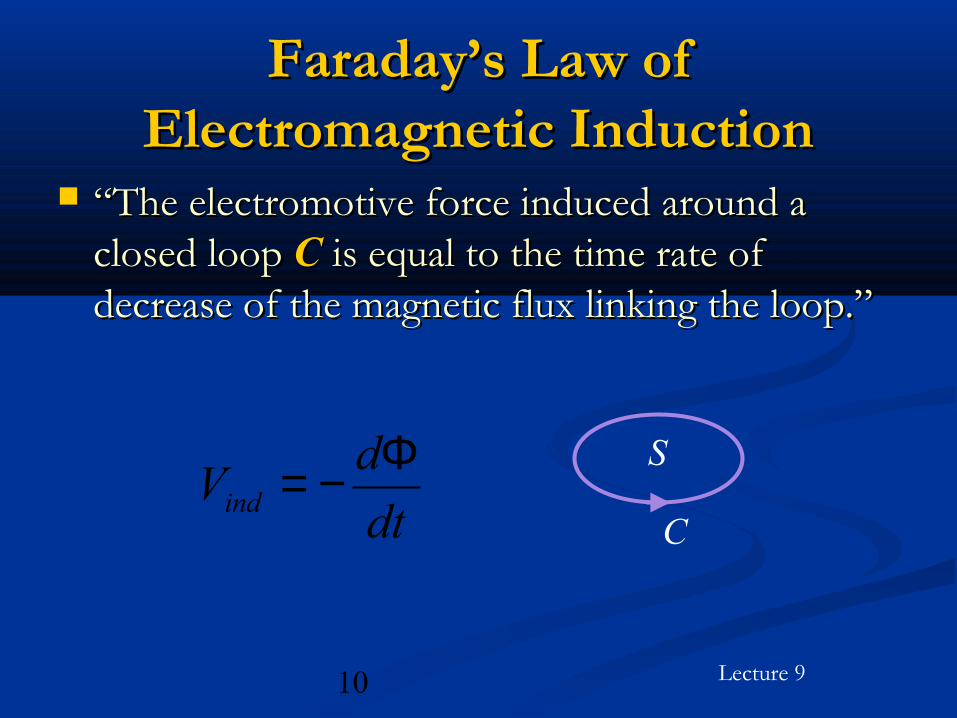
““The electromotive force induced around a The electromotive force induced around a closed loop closed loop CC is equal to the time rate of is equal to the time rate of decrease of the magnetic flux linking the loop.”decrease of the magnetic flux linking the loop.”
C
S
dt
dVind
Φ−=

11 Lecture 9
Faraday’s Law of Electromagnetic Faraday’s Law of Electromagnetic Induction (Cont’d)Induction (Cont’d)
∫ ⋅=ΦS
sdB• S is any surface bounded by C∫ ⋅=
C
ind ldEV
∫∫ ⋅−=⋅SC
sdBdt
dldE
integral form of Faraday’s
law

12 Lecture 9
Faraday’s Law (Cont’d)Faraday’s Law (Cont’d)
∫∫
∫∫
⋅∂∂−=⋅−
⋅×∇=⋅
SS
SC
sdt
BsdB
dt
d
sdEldE
Stokes’s theorem
assuming a stationary surface S

13 Lecture 9
Faraday’s Law (Cont’d)Faraday’s Law (Cont’d)
Since the above must hold for any Since the above must hold for any SS, we have, we have
t
BE
∂∂−=×∇
differential form of Faraday’s law
(assuming a stationary frame
of reference)
14 Lecture 9
Faraday’s Law (Cont’d)Faraday’s Law (Cont’d)
Faraday’s law states that a changing Faraday’s law states that a changing magnetic field induces an electric field.magnetic field induces an electric field.
The induced electric field is The induced electric field is non-non-conservativeconservative..
15 Lecture 9
Lenz’s LawLenz’s Law
““The sense of the emf induced by the time-The sense of the emf induced by the time-varying magnetic flux is such that any current it varying magnetic flux is such that any current it produces tends to set up a magnetic field that produces tends to set up a magnetic field that opposes the opposes the changechange in the original magnetic in the original magnetic field.”field.”
Lenz’s law is a consequence of conservation of Lenz’s law is a consequence of conservation of energy.energy.
Lenz’s law explains the minus sign in Faraday’s Lenz’s law explains the minus sign in Faraday’s law.law.

16 Lecture 9
Faraday’s LawFaraday’s Law ““The electromotive force induced around a The electromotive force induced around a
closed loop closed loop CC is equal to the time rate of is equal to the time rate of decrease of the magnetic flux linking the decrease of the magnetic flux linking the loop.”loop.”
For a coil of N tightly wound turnsFor a coil of N tightly wound turns
dt
dVind
Φ−=
dt
dNVind
Φ−=

17 Lecture 9
∫ ⋅=ΦS
sdB
• S is any surface bounded by C∫ ⋅=
C
ind ldEV
Faraday’s Law (Cont’d)Faraday’s Law (Cont’d)
C
S
18 Lecture 9
Faraday’s Law (Cont’d)Faraday’s Law (Cont’d)
Faraday’s law applies to situations whereFaraday’s law applies to situations where (1) the (1) the BB-field is a function of time-field is a function of time (2) (2) ddss is a function of time is a function of time (3) (3) BB and and ddss are functions of time are functions of time

19 Lecture 9
Faraday’s Law (Cont’d)Faraday’s Law (Cont’d)
The induced The induced emfemf around a circuit can be around a circuit can be separated into two terms:separated into two terms: (1) due to the time-rate of change of the B-(1) due to the time-rate of change of the B-
field (field (transformer emftransformer emf)) (2) due to the motion of the circuit ((2) due to the motion of the circuit (motional motional
emfemf))

20 Lecture 9
Faraday’s Law (Cont’d)Faraday’s Law (Cont’d)
( )∫∫
∫
⋅×+⋅∂∂−=
⋅−=
CS
S
ind
ldBvsdt
B
sdBdt
dV
transformer emfmotional emf
21 Lecture 9
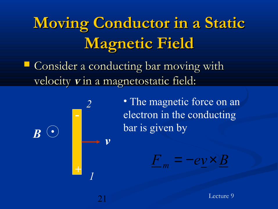
Moving Conductor in a Static Moving Conductor in a Static Magnetic FieldMagnetic Field
Consider a conducting bar moving with Consider a conducting bar moving with velocity velocity vv in a magnetostatic field: in a magnetostatic field:
Bv
2
1+
-• The magnetic force on an electron in the conducting bar is given by
BveF m ×−=

22 Lecture 9
Moving Conductor in a Static Moving Conductor in a Static Magnetic Field (Cont’d)Magnetic Field (Cont’d)
Electrons are pulled Electrons are pulled toward end toward end 22. End . End 22 becomes negatively becomes negatively charged and end charged and end 11 becomes becomes ++ charged. charged.
An electrostatic force An electrostatic force of attraction is of attraction is established between the established between the two ends of the bar.two ends of the bar.
Bv
2
1+
-

23 Lecture 9
Moving Conductor in a Static Moving Conductor in a Static Magnetic Field (Cont’d)Magnetic Field (Cont’d)
The electrostatic force on an electron The electrostatic force on an electron due to the induced electrostatic field is due to the induced electrostatic field is given bygiven by
The migration of electrons stops The migration of electrons stops (equilibrium is established) when(equilibrium is established) when
EeF e −=
BvEFF me ×−=⇒−=
24 Lecture 9
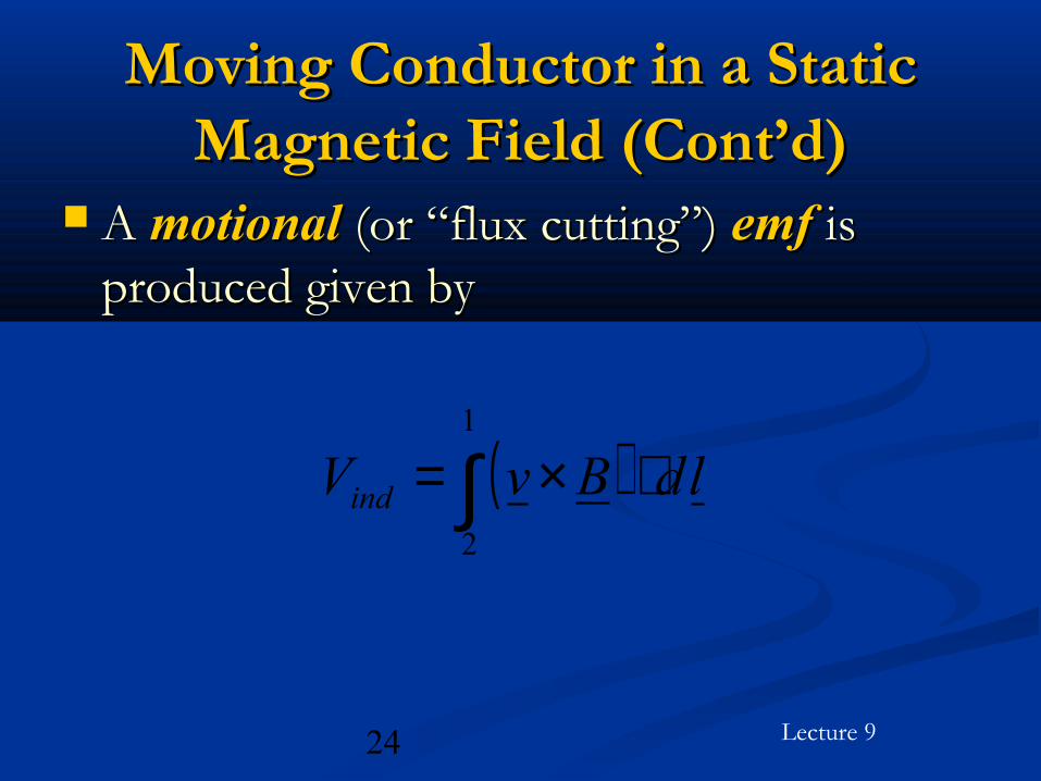
Moving Conductor in a Static Moving Conductor in a Static Magnetic Field (Cont’d)Magnetic Field (Cont’d)
A A motionalmotional (or “flux cutting”) (or “flux cutting”) emfemf is is produced given byproduced given by
( ) ldBvVind ⋅×= ∫1
2

25 Lecture 9
Electric Field in Terms of Electric Field in Terms of Potential FunctionsPotential Functions
Electrostatics:Electrostatics:
Φ−∇=⇒=×∇ EE 0
scalar electric potential

26 Lecture 9
Electric Field in Terms of Electric Field in Terms of Potential Functions (Cont’d)Potential Functions (Cont’d)
Electrodynamics:Electrodynamics:
( )
Φ−∇=∂∂+⇒=
∂∂+×∇
×∇∂∂−=
∂∂−=×∇
t
AE
t
AE
Att
BE
0
AB ×∇=

27 Lecture 9
Electric Field in Terms of Electric Field in Terms of Potential Functions (Cont’d)Potential Functions (Cont’d)
Electrodynamics:Electrodynamics:
t
AE
∂∂−Φ−∇=
scalar electric
potential
vector magnetic potential
• both of these potentials are now functions of time.

28 Lecture 9
The differential form of Ampere’s law in The differential form of Ampere’s law in the static case isthe static case is
The continuity equation isThe continuity equation is
JH =×∇
0=∂
∂+⋅∇t
qJ ev
Ampere’s Law and the Continuity Ampere’s Law and the Continuity EquationEquation
29 Lecture 9
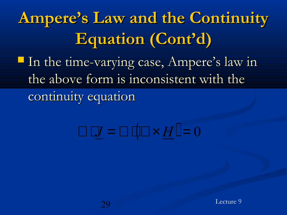
Ampere’s Law and the Continuity Ampere’s Law and the Continuity Equation (Cont’d)Equation (Cont’d)
In the time-varying case, Ampere’s law in In the time-varying case, Ampere’s law in the above form is inconsistent with the the above form is inconsistent with the continuity equationcontinuity equation
( ) 0=×∇⋅∇=⋅∇ HJ

30 Lecture 9
Ampere’s Law and the Continuity Ampere’s Law and the Continuity Equation (Cont’d)Equation (Cont’d)
To resolve this inconsistency, Maxwell To resolve this inconsistency, Maxwell modified Ampere’s law to readmodified Ampere’s law to read
t
DJH c ∂
∂+=×∇
conduction current density
displacement current density

31 Lecture 9
Ampere’s Law and the Continuity Ampere’s Law and the Continuity Equation (Cont’d)Equation (Cont’d)
The new form of Ampere’s law is The new form of Ampere’s law is consistent with the continuity equation as consistent with the continuity equation as well as with the differential form of well as with the differential form of Gauss’s lawGauss’s law
( ) ( ) 0=×∇⋅∇=⋅∇∂∂+⋅∇ HDt
J c
qev

32 Lecture 9
Displacement CurrentDisplacement Current
Ampere’s law can be written asAmpere’s law can be written as
dc JJH +=×∇
where
)(A/mdensity current nt displaceme 2=∂∂=
t
DJ d
33 Lecture 9
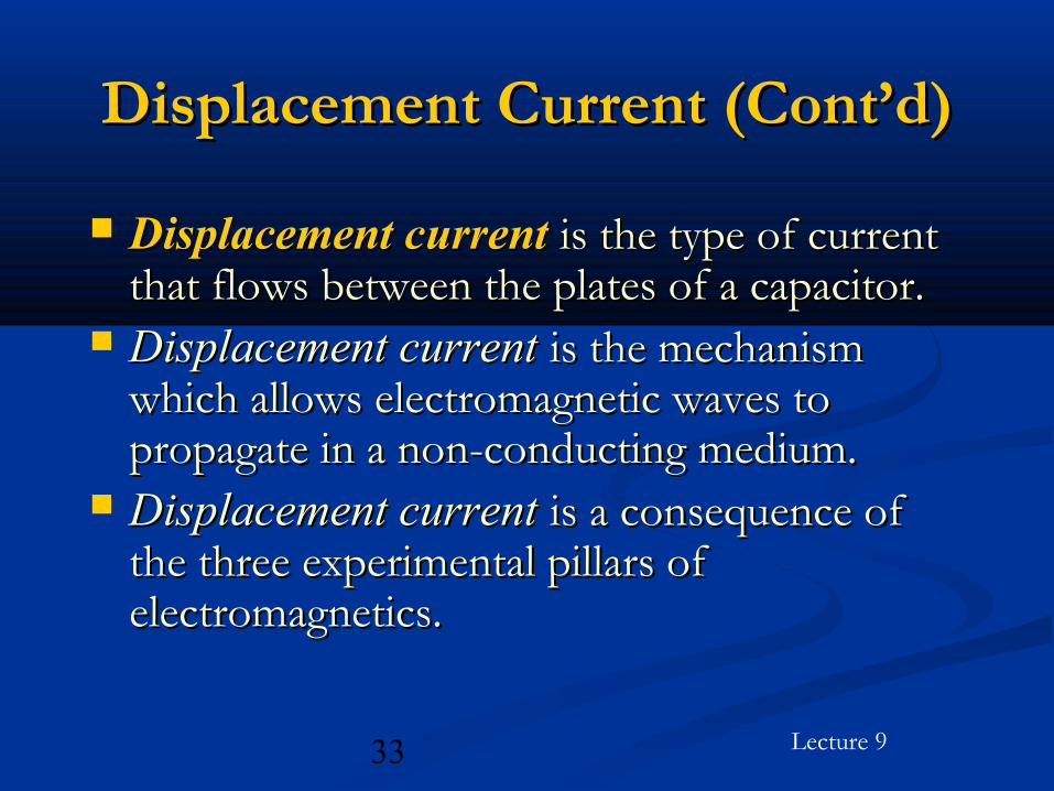
Displacement Current (Cont’d)Displacement Current (Cont’d)
Displacement currentDisplacement current is the type of current is the type of current that flows between the plates of a capacitor.that flows between the plates of a capacitor.
Displacement currentDisplacement current is the mechanism is the mechanism which allows electromagnetic waves to which allows electromagnetic waves to propagate in a non-conducting medium.propagate in a non-conducting medium.
Displacement currentDisplacement current is a consequence of is a consequence of the three experimental pillars of the three experimental pillars of electromagnetics.electromagnetics.
34 Lecture 9
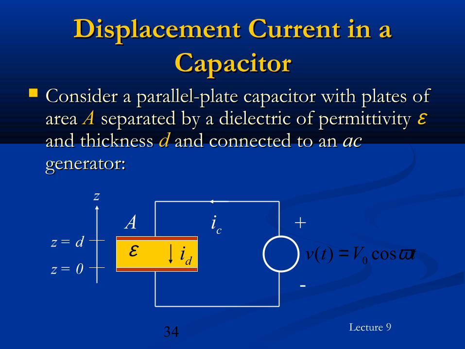
Displacement Current in a Displacement Current in a CapacitorCapacitor
Consider a parallel-plate capacitor with plates of Consider a parallel-plate capacitor with plates of area area AA separated by a dielectric of permittivity separated by a dielectric of permittivity εε and thickness and thickness dd and connected to an and connected to an acac generator:generator:
tVtv ωcos)( 0=+
-z = 0
z = d εicA
id
z
35 Lecture 9
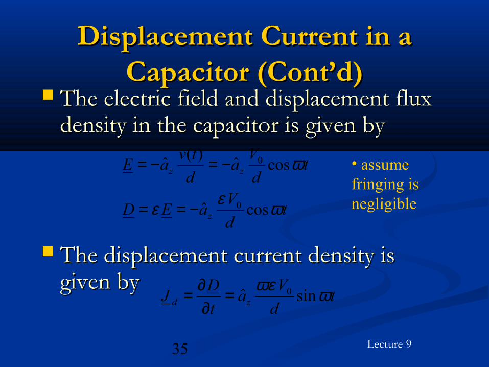
Displacement Current in a Displacement Current in a Capacitor (Cont’d)Capacitor (Cont’d)
The electric field and displacement flux The electric field and displacement flux density in the capacitor is given bydensity in the capacitor is given by
The displacement current density is The displacement current density is given bygiven by
td
VaED
td
Va
d
tvaE
z
zz
ωεε
ω
cosˆ
cosˆ)(
ˆ
0
0
−==
−=−= • assume fringing is negligible
td
Va
t
DJ zd ωωε
sinˆ 0=∂∂=

36 Lecture 9
c
d
S
dd
idt
dvCtCV
tVd
AAJsdJi
==−=
−=−=⋅= ∫
ωω
ωωε
sin
sin
0
0
Displacement Current in a Displacement Current in a Capacitor (Cont’d)Capacitor (Cont’d)
The displacement current is given byThe displacement current is given by
conduction current in
wire
37 Lecture 9
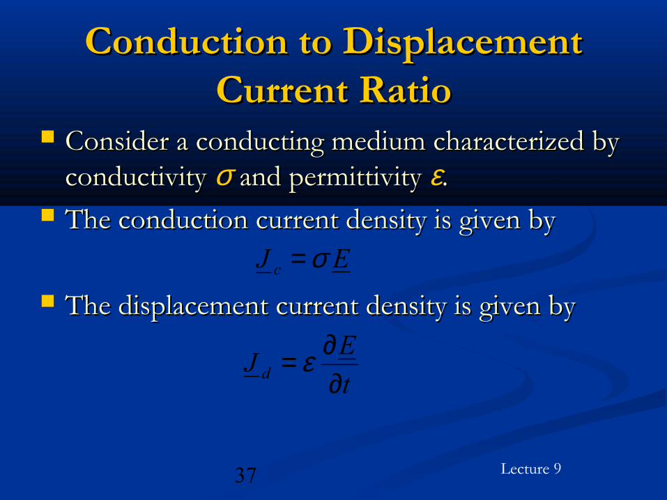
Conduction to Displacement Conduction to Displacement Current RatioCurrent Ratio
Consider a conducting medium characterized by Consider a conducting medium characterized by conductivity conductivity σσ and permittivity and permittivity εε..
The conduction current density is given byThe conduction current density is given by
The displacement current density is given byThe displacement current density is given by
EJ c σ=
t
EJ d ∂
∂= ε

38 Lecture 9
Conduction to Displacement Conduction to Displacement Current Ratio (Cont’d)Current Ratio (Cont’d)
Assume that the electric field is a sinusoidal Assume that the electric field is a sinusoidal function of time:function of time:
Then, Then, tEE ωcos0=
tEJ
tEJ
d
c
ωωεωσsin
cos
0
0
−==

39 Lecture 9
Conduction to Displacement Conduction to Displacement Current Ratio (Cont’d)Current Ratio (Cont’d)
We haveWe have
Therefore Therefore
0max
0max
EJ
EJ
d
c
ωε
σ
=
=
ωεσ=
max
max
d
c
J
J

40 Lecture 9
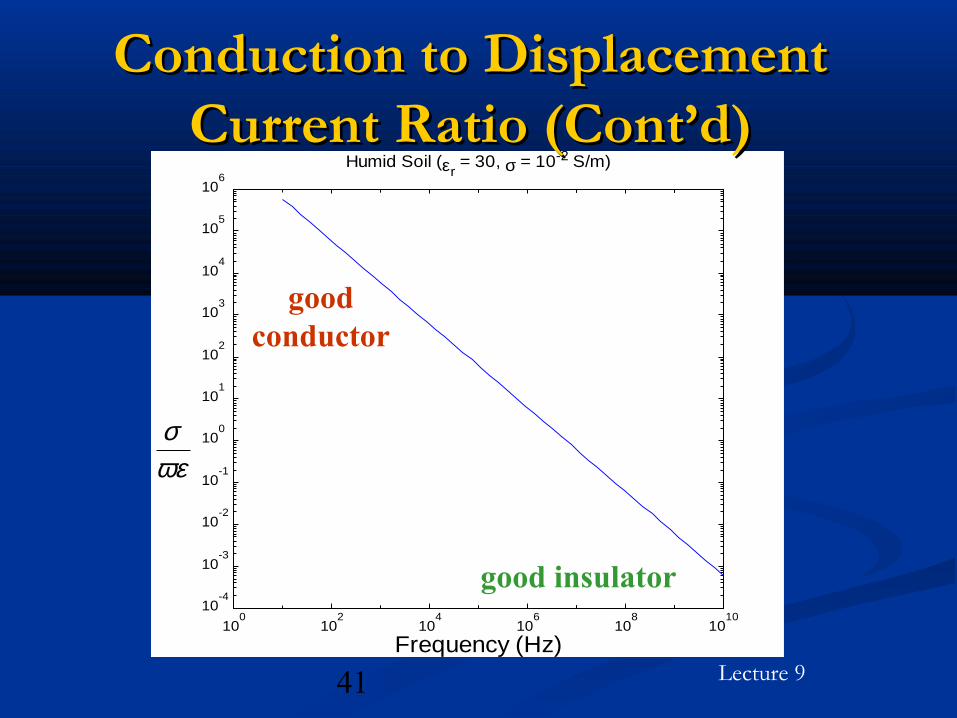
Conduction to Displacement Conduction to Displacement Current Ratio (Cont’d)Current Ratio (Cont’d)
The value of the quantity The value of the quantity σ/ωεσ/ωε at a specified at a specified frequency determines the properties of the frequency determines the properties of the medium at that given frequency.medium at that given frequency.
In a metallic conductor, the displacement In a metallic conductor, the displacement current is negligible below optical frequencies.current is negligible below optical frequencies.
In free space (or other perfect dielectric), the In free space (or other perfect dielectric), the conduction current is zero and only conduction current is zero and only displacement current can exist. displacement current can exist.
41 Lecture 9
100
102
104
106
108
1010
10-4
10-3
10-2
10-1
100
101
102
103
104
105
106
Frequency (Hz)
Humid Soil (εr = 30, σ = 10-2 S/m)
ωεσ
goodconductor
good insulator
Conduction to Displacement Conduction to Displacement Current Ratio (Cont’d)Current Ratio (Cont’d)
42 Lecture 9
Complex PermittivityComplex Permittivity
In a good insulator, the conduction current (due to In a good insulator, the conduction current (due to non-zero non-zero σσ) is usually negligible.) is usually negligible.
However, at high frequencies, the rapidly varying However, at high frequencies, the rapidly varying electric field has to do work against molecular forces electric field has to do work against molecular forces in alternately polarizing the bound electrons.in alternately polarizing the bound electrons.
The result is that The result is that PP is not necessarily in phase with is not necessarily in phase with EE, and the electric susceptibility, and hence the , and the electric susceptibility, and hence the dielectric constant, are complex.dielectric constant, are complex.
43 Lecture 9
Complex Permittivity (Cont’d)Complex Permittivity (Cont’d)
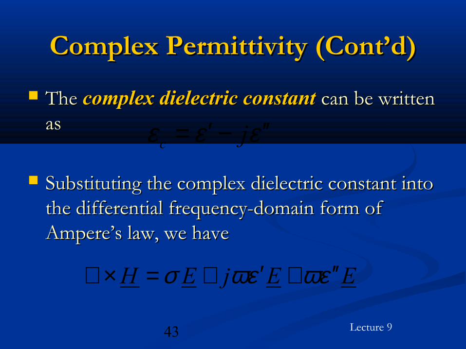
The The complex dielectric constantcomplex dielectric constant can be written can be written asas
Substituting the complex dielectric constant into Substituting the complex dielectric constant into the differential frequency-domain form of the differential frequency-domain form of Ampere’s law, we haveAmpere’s law, we have
εεε ′′−′= jc
EEjEH εωεωσ ′′+′+=×∇

44 Lecture 9
Complex Permittivity (Cont’d)Complex Permittivity (Cont’d) Thus, the imaginary part of the complex Thus, the imaginary part of the complex
permittivity leads to a volume current density permittivity leads to a volume current density term that is in phase with the electric field, as term that is in phase with the electric field, as if the material had an effective conductivity if the material had an effective conductivity given bygiven by
The power dissipated per unit volume in the The power dissipated per unit volume in the medium is given bymedium is given by
εωσσ ′′+=eff
222 EEEeff εωσσ ′′+=

45 Lecture 9
Complex Permittivity (Cont’d)Complex Permittivity (Cont’d)
The term The term ωε′′ ωε′′ EE22 is the basis for microwave is the basis for microwave heating of dielectric materials.heating of dielectric materials.
Often in dielectric materials, we do not Often in dielectric materials, we do not distinguish between distinguish between σσ and and ωε′′ωε′′, and lump them , and lump them together in together in ωε′′ωε′′ as as
effσεω =′′• The value of σeff is often determined by
measurements.
46 Lecture 9
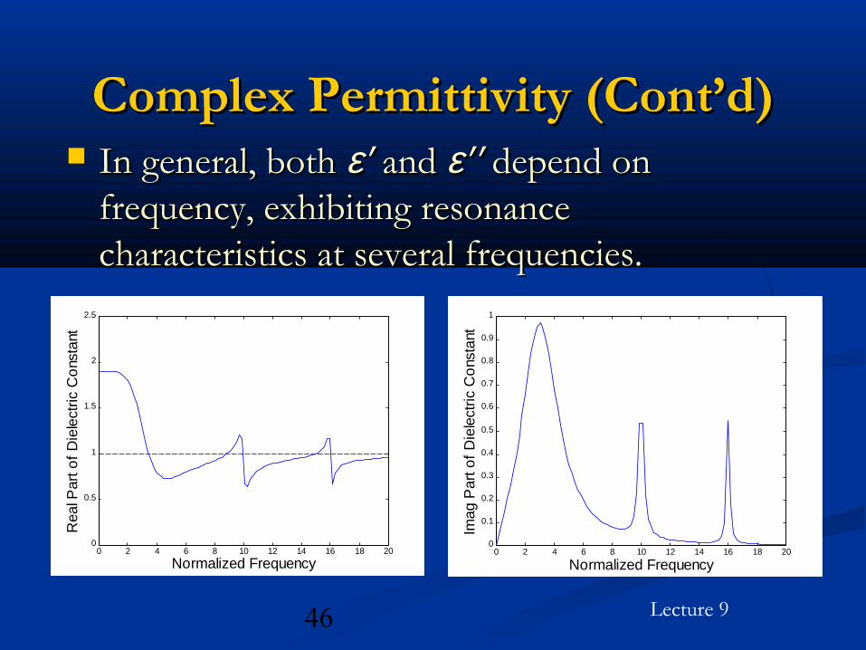
Complex Permittivity (Cont’d)Complex Permittivity (Cont’d) In general, both In general, both ε′ε′ and and ε′′ε′′ depend on depend on
frequency, exhibiting resonance frequency, exhibiting resonance characteristics at several frequencies. characteristics at several frequencies.
0 2 4 6 8 10 12 14 16 18 200
0.5
1
1.5
2
2.5
Normalized Frequency
Rea
l Par
t of
Die
lect
ric C
ons
tant
0 2 4 6 8 10 12 14 16 18 200
0.1
0.2
0.3
0.4
0.5
0.6
0.7
0.8
0.9
1
Normalized Frequency
Imag
Par
t of
Die
lect
ric C
ons
tant

47 Lecture 9
Complex Permittivity (Cont’d)Complex Permittivity (Cont’d)
In tabulating the dielectric properties of In tabulating the dielectric properties of materials, it is customary to specify the real part materials, it is customary to specify the real part of the dielectric constant (of the dielectric constant (ε′ε′ / / εε00) and the loss ) and the loss
tangent (tangent (tantanδδ) defined as) defined as
εεδ
′′′
=tan
48 Lecture 9
Complex PermeabilityComplex Permeability
Like the electric field, the magnetic field Like the electric field, the magnetic field encounters molecular forces which require work encounters molecular forces which require work to overcome in magnetizing the material.to overcome in magnetizing the material.
In analogy with permittivity, the permeability In analogy with permittivity, the permeability can also be complex can also be complex
µµµ ′′−′= jc
49 Lecture 9
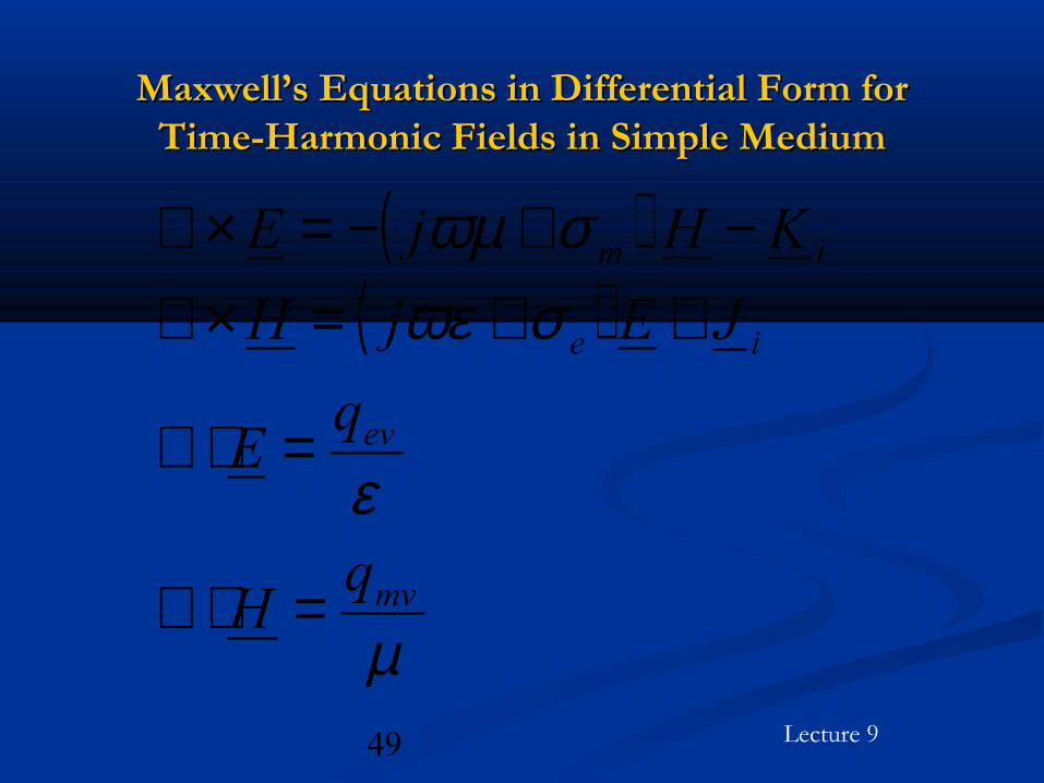
Maxwell’s Equations in Differential Form for Maxwell’s Equations in Differential Form for Time-Harmonic Fields in Simple MediumTime-Harmonic Fields in Simple Medium
( )( )
µ
ε
σωεσωµ
mv
ev
ie
im
qH
qE
JEjH
KHjE
=⋅∇
=⋅∇
++=×∇−+−=×∇
50 Lecture 9
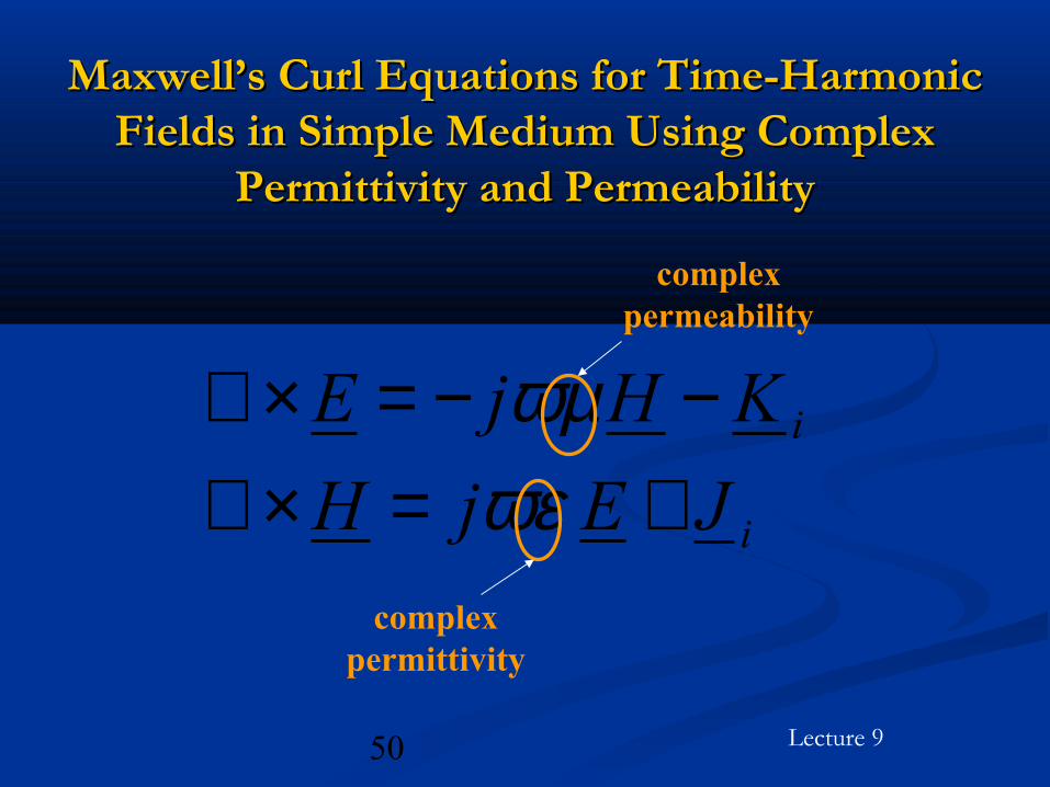
Maxwell’s Curl Equations for Time-Harmonic Maxwell’s Curl Equations for Time-Harmonic Fields in Simple Medium Using Complex Fields in Simple Medium Using Complex
Permittivity and PermeabilityPermittivity and Permeability
i
i
JEjH
KHjE
+=×∇−−=×∇
ωεωµ
complexpermittivity
complexpermeability


![Lect09-CN303 [Compatibility Mode]](https://static.fdocuments.us/doc/165x107/577d1d351a28ab4e1e8bd1d8/lect09-cn303-compatibility-mode.jpg)