LEANING AGAINST THE WIND - World Bank
57
Semiannual Report • Office of the Regional Chief Economist April 2017 FISCAL POLICY IN LATIN AMERICA AND THE CARIBBEAN IN A HISTORICAL PERSPECTIVE LEANING AGAINST THE WIND
Transcript of LEANING AGAINST THE WIND - World Bank

Semiannual Report • Office of the Regional Chief Economist April 2017
The World Bank1818 H Street, NW,Washington, DC 20433, USA.www.worldbank.org/laceconomist
FISCAL POLICY IN LATIN AMERICA AND THE CARIBBEAN IN A HISTORICAL PERSPECTIVE
LEANING AGAINST THE WIND

Leaning Against the Wind:
Fiscal Policy in Latin America and the Caribbean in a Historical Perspective

© 2017 International Bank for Reconstruction and Development / The World Bank
1818 H Street NW, Washington DC 20433
Telephone: 202-473-1000; Internet: www.worldbank.org
Some rights reserved
1 2 3 4 20 19 18 17
This work is a product of the staff of The World Bank with external contributions. The findings, interpretations, and conclusions expressed in this work do not necessarily reflect the views of The World Bank, its Board of Executive Directors, or the governments they represent. The World Bank does not guarantee the accuracy of the data included in this work. The boundaries, colors, denominations, and other information shown on any map in this work do not imply any judgment on the part of The World Bank concerning the legal status of any territory or the endorsement or acceptance of such boundaries.
Nothing herein shall constitute or be considered to be a limitation upon or waiver of the privileges and immunities of The World Bank, all of which are specifically reserved.
Rights and Permissions
This work is available under the Creative Commons Attribution 3.0 IGO license (CC BY 3.0 IGO) http://creativecommons.org/licenses/by/3.0/igo. Under the Creative Commons Attribution license, you are free to copy, distribute, transmit, and adapt this work, including for commercial purposes, under the following conditions:
Attribution—Please cite the work as follows: Carlos Vegh, Daniel Lederman, and Federico R. Bennet. 2017. “Leaning against the Wind: Fiscal Policy in Latin America and the Caribbean in a Historical Perspective.” LAC Semiannual Report (April), Washington, DC: World Bank. Doi: 10.1596/978-1-4648-1094-7. License: Creative Commons Attribution CC BY 3.0 IGO
Translations—If you create a translation of this work, please add the following disclaimer along with the attribution: This translation was not created by The World Bank and should not be considered an official World Bank translation. The World Bank shall not be liable for any content or error in this translation.
Adaptations—If you create an adaptation of this work, please add the following disclaimer along with the attribution: This is an adaptation of an original work by The World Bank. Views and opinions expressed in the adaptation are the sole responsibility of the author or authors of the adaptation and are not endorsed by The World Bank.
Third-party content—The World Bank does not necessarily own each component of the content contained within the work. The World Bank therefore does not warrant that the use of any third-party-owned individual component or part contained in the work will not infringe on the rights of those third parties. The risk of claims resulting from such infringement rests solely with you. If you wish to re-use a component of the work, it is your responsibility to determine whether permission is needed for that re-use and to obtain permission from the copyright owner. Examples of components can include, but are not limited to, tables, figures, or images.
All queries on rights and licenses should be addressed to World Bank Publications, The World Bank Group, 1818 H Street NW, Washington, DC 20433, USA; e-mail: [email protected].
ISBN (electronic): 978-1-4648-1094-7
DOI: 10.1596/ 978-1-4648-1094-7
Cover design: Kilka Diseño Gráfico.

| 3
Acknowledgements
This report was prepared by a core team composed of Carlos A. Végh (Regional Chief Economist), Daniel Lederman (Regional Deputy Chief Economist) and Federico R. Bennett (Research Analyst). The authors gratefully acknowledge the comments and support provided by numerous colleagues that greatly helped improve this report. Members of the World Bank’s Regional Management Team for Latin America and the Caribbean asked tough questions and provided invaluable insights during a presentation that took place on March 23, 2017. A team of country economists working under the supervision of Pablo Saavedra and Miria Pigato (Practice Managers for Macroeconomics and Fiscal Management), particularly Cristina Savescu, offered useful comments. Stellar research assistance was provided by Agamemnon Koutsogiorgas and Martin Sasson. Samuel Pienknagura (Senior Economist), Justin Lesniak (Research Analyst), and Luis Morano Germani (Research Analyst) provided fresh eyes during key moments prior to the completion of the report. Guillermo Vuletin (IDB) kindly provided helpful feedback on Chapter 2. The authors also received insightful comments from a large number of macroeconomists and country economists of the World Bank Group’s Macroeconomics and Fiscal Management Global Practice, who attended a preliminary presentation of the findings on March 27, 2017. Alejandra Viveros (Manager, External Communications) and Marcela Sanchez-Bender (Communications Officer) provided constant feedback that made this report more accessible to non-economists. Finally, this report would not have come to be without the unfailing administrative support of Ruth Delgado and Jacqueline Larrabure.
April 2017

4 | Leaning Against the Wind

| 5
Executive Summary
After a slowdown that has lasted six years (including two consecutive years of negative growth in 2015 and 2016), the market analysts expect that the Latin American and Caribbean (LAC) region will grow in 2017 by around 1.5 percent, followed by 2.5 percent in 2018. The slowdown since 2011 (and contraction in the last two years) has been driven essentially by the performance of some of the large South American (SA) economies (particularly Argentina, Brazil, and Venezuela, RB), with Brazil posting its second straight year of negative growth (-3.8 percent in 2015 and -3.6 percent in 2016) and Venezuela’s GDP falling by a staggering 12 percent in 2016. Mexico’s growth is expected to reach 2 percent by 2018 and Central America and the Caribbean are expected to continue to grow at a steady pace of around 3.8 percent, as has been the case since the Global Financial Crisis.
A notable feature of this long slowdown has been the deterioration of the fiscal accounts, even in sub-regions, such as Mexico, Central America, and the Caribbean (MCC), where the deceleration has been much less pronounced than in SA. In fact, 29 of 32 countries in the region had an overall fiscal deficit in 2016. The median deficit for SA in 2016 was 5.2 percent of GDP, compared to 2.1 percent for MCC. As a result of the build-up of fiscal deficits, debt stocks have been rising over the years, reaching a median gross debt of 50 percent of GDP for the region as a whole, with countries such as Jamaica and Barbados reaching debt levels of 119 and 105 percent of GDP, respectively. Such a delicate fiscal situation, which severely constrains the macroeconomic and public policy choices of many countries in the region, is the focus of this report. The aim is to, first, understand how we got here and, second, how to think about the fiscal choices that different countries may face.
To see fiscal deficits increase during a slowdown or recession should, of course, not surprise us. Even if the fiscal authority were completely passive and kept government spending and tax rates constant, the endogenous fall in the tax base (consumption and/or income) resulting from the recession itself would reduce tax revenues considerably and hence increase fiscal deficits. This is a helpful conceptual benchmark because it already tells us that, in and of themselves, fiscal deficits are not necessarily bad. The days in which the mere sight of a fiscal deficit would automatically trigger an adjustment should be long gone, and rightly so. As this report will make clear, however, reality is always more complicated and even before asking the question of whether and how much a country should adjust, we need to understand how we got to this situation (the focus of Chapter 1), how fiscal policy is conducted over the business cycle (Chapter 2), and the links between fiscal policy, debt sustainability, and duration of shocks (Chapter 2). Only after answering these questions can practitioners decide whether and by how much fiscal accounts should be adjusted.
How did we get here? In SA, the median fiscal deficit in 2016 was 4.6 percent of GDP higher than in 2011. Interestingly enough, while the median fall in revenues during the same period was 1.4 percent, the median increase in expenditures was 3.6 percent of GDP. In other words, were it not for a substantial increase in spending, fiscal accounts would have deteriorated much less. In contrast, and reflecting the much more stable path of GDP during the same period, MCC experienced a slight fall in the median fiscal deficit of 0.8 percent of GDP, with a median decrease of expenditure of 0.4 percent of GDP and a median increase in revenues of 1.4 percent of GDP. As detailed in Chapter

6 | Leaning Against the Wind
1, even when looking at accumulated public expenditures since the year 2000, the median for SA countries was 39 percent of 2000 GDP compared to 33 percent of 2000 GDP for MCC. While MCC relied much more on debt as a source of financing, SA could count on higher revenues, generated by a combination of growth and relatively higher revenue rates. In sum, we learn from Chapter 1 that even though SA and MCC followed quite different fiscal paths since the year 2000, they find themselves in a similar fiscal quagmire in early 2017: high fiscal deficits and large stocks of debt, with the prospect of having to find further fiscal cuts in the midst of low growth (particularly in SA) and policy uncertainty (particularly for MCC).
Having established the basic fiscal facts in Chapter 1, Chapter 2 – the core of the report – analyzes in detail the main fiscal forces that have come into play and shaped fiscal policy as a macroeconomic tool in developing countries in general, and LAC in particular. To this effect, we go back in time and look for basic patterns that may guide us in our quest to understand fiscal policy. The first question to be asked is: how has fiscal policy been conducted over the business cycle during the last 5 decades or so? The evidence shows that, by and large, fiscal policy in developing countries, and LAC in particular, has been procyclical (in fact, the only LAC country that has not been historically procyclical is El Salvador). In other words, fiscal policy has typically been expansionary in good times and contractionary in bad times. Importantly, this is exactly the opposite of what transpires in industrial countries, where fiscal policy has almost always been countercyclical (expansionary in bad times and contractionary in good times). Procyclical fiscal policy is clearly undesirable as it amplifies the already volatile business cycle of LAC countries by making the booms larger and the recessions deeper. So why would the fiscal authority follow such a policy? We conjecture that political economy pressures for more spending in good times coupled with limited access to international credit markets in bad times lie at the heart of this fiscal procyclicality trap.
The question then arises: have some countries been able to switch from procyclical to countercyclical fiscal policy over time? The answer is a definite yes. In fact, if the 1960-2016 period is split before and after the year 2000, 41 percent of formerly procyclical countries were able to switch to countercyclical policies (this number is 39 percent for LAC countries). Whether a country is procyclical or countercyclical is clearly key to understanding its fiscal behavior over the business cycle. If a country is countercyclical, then fiscal deficits in bad times may be partly due to an attempt to stimulate the economy through higher spending and/or lower tax rates. This would explain large increases in spending during 2008-2009 in countries such as Chile, Colombia and Mexico, as a way to stimulate the economy during the Global Financial Crisis. Chile, in particular, enacted a fiscal stimulus package equivalent to 2.8 percent of GDP, roughly the same order of magnitude as the one implemented in the United States.
Based on this fiscal framework, Chapter 2 proceeds to examine the recent fiscal behavior of many LAC countries through the lenses of procyclical versus countercyclical fiscal policy in order to understand the challenges that lie ahead. While, in the last decade, Chile, Colombia, Guatemala, Mexico, Paraguay, and Peru have become countercyclical, countries like Argentina, Bolivia, Brazil, Nicaragua, Panama, and Uruguay have continued to be procyclical. If growth continues to be sluggish, life will clearly be more difficult for the latter group than for the former. In particular, the countercyclical group will have some fiscal space to deploy public expenditures as a stimulus tool, a luxury that the procyclical group will not have.
The report then asks a critical question: is there a link between fiscal procyclicality and debt sustainability? While, in theory, such a link is not necessarily part of the picture, in practice, more procyclical countries tend to have lower credit ratings, suggesting riskier public debt positions. This is not surprising since, by definition, a procyclical country will find itself trying to cut spending in bad times, which is certainly a hard political feat to achieve. Procyclical countries, therefore,
| 7
will need to consolidate the fiscal accounts further than otherwise in order to minimize the risks of a deterioration in their credit ratings and hence an increase in credit costs.
Finally, the report explores the possible link between procyclicality and the duration of shocks. In theory, a country should adjust to a negative permanent shock (i.e., should cut expenditure by the same amount as the shock) but can “finance” a temporary shock (i.e., can borrow to keep expenditures roughly constant and repay when good times come back). In practice, of course, policymakers face the extraordinarily difficult situation of needing to assess the possible duration of the shock in real time. This has been a particularly challenging task to handle for commodity exporters once commodity prices started to fall drastically in 2014.
By examining how Chile handles its estimates of the “reference” price for copper (which can be viewed as the estimate of the long-run or “permanent” price of copper), the report argues that prudence is probably the only practical policy choice. By definition, a prudent policymaker will tend to put more weight on a positive shock being temporary and a negative shock being permanent. As a result, the prudent policymaker may, on average, save too much in good times and dis-save (or borrow) too little in bad times. This “excessive” saving could be viewed as the cost of self-insurance, and hence a price that needs to be paid for living in shock-prone or more volatile external environments. Interestingly enough, in bad times a prudent policymaker may mimic, to some extent at least, a procyclical policymaker. But, if anything, this should be viewed as an additional argument to seek the blessings of countercyclical fiscal policies since market-based insurance (which would clearly be the first-best scenario) should be more readily available to countries with higher credit ratings.

8 | Leaning Against the Wind

| 9
Introduction
Gross domestic product (GDP) in the Latin American and Caribbean (LAC) region fell by 1.0 percent in 2016. This negative regional growth rate was driven by the lackluster performance of four relatively large economies: Venezuela, RB (-12.0 percent), Brazil (-3.6 percent), Argentina (-2.3 percent), and Ecuador (-2.1 percent), which together account for around 54 percent of the region’s GDP. However, three small economies that are also net exporters of commodities (Suriname, Trinidad and Tobago, and Belize) experienced GDP contractions in 2016 as well. Thus, the adjustment processes triggered by the end of the commodity boom a few years ago are still being felt throughout the region, engulfing large and small economies alike.
Nonetheless, Consensus Forecasts indicate that the region is expected to grow by about 1.5 percent in 2017, due primarily to a modest recovery in Brazil (0.7 percent growth) and growth of 3.0 percent in Argentina. In fact, these forecasts suggest that only Venezuela, RB is expected to face a contraction in 2017, with GDP falling by 3.1 percent. These forecasts, however, might end up being off the mark, as it is clear that LAC is still not out of the woods yet. In particular, LAC economies are facing important fiscal challenges that have yet to be fully absorbed, as most regional economies ended 2016 with fiscal deficits.1 This report is thus focused on the fiscal issues that have emerged in the aftermath of the global economic slowdown that has been the subject of several previous installments of this LAC semiannual macro-report series (see, for example, de la Torre et al. 2015a and de la Torre et al. 2016).
As in past editions of this semiannual series, the rest of this report is organized around two chapters. The first reviews the growth prospects of the region for 2016 and 2017 in light of its performance since the beginning of the 21st century and of the performance of the global economy. As the global economy has slowed down since 2011, the LAC region has faced various challenges, including fiscal pressures especially in commodity-dependent economies ranging from Mexico and Colombia to Trinidad and Tobago. In this context, Chapter 1 examines how rising public sector expenditures were funded and financed since 2000. This analysis of the origins of the current fiscal challenges facing LAC economies is capped by a descriptive assessment of the ensuing process of fiscal adjustments
1 In this report, South America includes all economies located south and east of Panama, including Trinidad and Tobago, Suriname and Guyana. The economies from Mexico, Central America and the (geographic) Caribbean include the following: Antigua and Barbuda, the Bahamas, Barbados, Belize, Costa Rica, Dominica, Dominican Republic, El Salvador, Grenada, Guatemala, Haiti, Honduras, Jamaica, Mexico, Nicaragua, Panama, St. Kitts and Nevis, St. Lucia, and St. Vincent and the Grenadines. These definitions differ from the World Bank country group definitions in which Trinidad and Tobago, Suriname and Guyana are grouped under the Caribbean.

10 | Leaning Against the Wind
that took place in most economies, from South America to Mexico, Central America, and the Caribbean.
The fact that most LAC economies are currently facing fiscal deficits is where the similarities among this diverse group of economies end because, in principle, the need for fiscal adjustment will depend on various factors, such as the state of the business cycle, debt sustainability, and the duration of specific shocks, all of which may vary across countries. The second chapter, which is the heart of the report, thus analyzes the cyclical properties of fiscal policy in LAC from a historical perspective. More specifically, it provides an overview of the cyclical properties of LAC fiscal policies since the 1960s, which highlights the tendency of developing economies to exhibit procyclical fiscal policies, on both the expenditure and taxation sides of the fiscal balance. Procyclical fiscal policy implies that fiscal policy is expansionary in good times and contractionary in bad times, which can lead to the amplification of economic cycles.
Yet, several LAC economies, including Chile, Costa Rica, Mexico, and Paraguay seem to have shifted towards countercyclical spending policies during the 21st century, particularly in response to the Global Financial Crisis of 2008/9. Chapter 2 points out, however, that the shift towards countercyclical fiscal policy does not, by itself, ensure that fiscal policy will be on a sustainable path. While, in theory, there is no necessary relationship between the cyclical properties of fiscal spending and debt sustainability, the evidence indicates that there is. Specifically, economies with more procyclical fiscal policy tend to have worse credit ratings.
Finally, the chapter explores a very important practical consideration: to properly conduct fiscal policy over the business cycle, policymakers should be able to ascertain if a shock is temporary or permanent. As is well-known, governments should adjust to a permanent negative shock but borrow to finance a temporary one. In practice, however, the duration of any particular shock is rather hard to evaluate. We argue that a “prudent” policymaker should tend to think of positive shocks as temporary and negative shocks as permanent and will thus tend to save more in good times and dis-save less (or borrow less) in bad times. While this “excess” saving could be viewed as the cost of self-insuring, it is interesting to note that the prudent policymaker will appear to act procyclically in bad times.

| 11
Chapter 1: Growth, Adjustments, and Financing Needs in the 21st Century
Introduction This chapter provides a bird’s eye view of recent growth performance and Consensus Forecasts for most economies of the region. It includes a comparison with past medium-term growth rates and a focus on the role of external drivers of LAC growth. As the external drivers of growth have subsided, without any evidence that these trends are likely to be reversed any time soon, it is likely that domestic factors, including fiscal policies, have become more important as drivers of growth across all of LAC. These issues are covered in the following section.
In turn, the chapter analyzes how rising government expenditures were either funded by rising public revenues or financed by increases in net debt. Countries with high revenue rates and/or high average growth rates since 2000 tended to accumulate less public debt than economies that did not benefit from a growth spurt. After the global and regional growth slowdowns took root around 2011, LAC economies faced challenges associated with fiscal adjustments. This occurred to varying degrees and with notable heterogeneity within LAC. Roughly speaking, economies from South America (SA) generally have higher primary fiscal deficits than the typical economy from Mexico, Central America, and the Caribbean (MCC), with a few exceptions that are discussed in detail below. Also, the Caribbean and Central American economies tend to face issues related to interest payments on accumulated debt to a greater extent, but again with notable exceptions that are discussed below.
LAC Growth Performance in the 21st Century As already mentioned, the LAC region is expected to grow by about 1.5 percent in 2017. This modest rebound, however, is coming on the heels of a protracted slowdown that began around 2011. As discussed in previous installments of this series, this slowdown was surprising in that the realized growth rates since then have tended to come in below market expectations. In other words, even though the slowdown percolated gradually throughout LAC, its longevity and depth were somewhat surprising.
In terms of the slowdown, it is reasonable to ask if global factors were behind it. Figure 1.1 shows the GDP growth rates of LAC alongside those of major global economies and other middle-income

12 | Leaning Against the Wind
FIGURE 1.1. Regional GDP Growth Rates since 2003 and Consensus Forecasts for 2017
Notes: 2016 values are estimates; 2017 values are forecasts. Sub-regional values are weighted averages or medians. SA includes Venezuela, RB, Suriname, Trinidad and Tobago, Brazil, Argentina, Ecuador, Uruguay, Chile, Colombia, Guyana, Paraguay, Bolivia, and Peru. CC includes Belize, St. Lucia, The Bahamas, Barbados, Haiti, Dominica, Jamaica, St. Vincent and the Grenadines, El Salvador, Antigua and Barbuda, Grenada, St. Kitts and Nevis, Guatemala, Honduras, Costa Rica, Nicaragua, Panama, and Dominican Republic. LAC Small Economies include LAC countries that have less than 5M workers. MIC denotes Middle Income Countries. Sources: Consensus Forecasts, World Bank’s GEP, and WEO.
economies from Europe and Central Asia (ECA) and South East Asia (SEA).2 The bars on the left-hand side (LHS) of the figure are weighted averages for each group, whereas the last four bar charts on the right-hand side (RHS) of the figure correspond to the median (or typical) country in four LAC groupings, namely LAC, South America, Central America and the Caribbean (CC), and the small economies of LAC (defined as any economy with less than five million workers, which corresponds to the median size across the world).3
For all cases, we show the average annual growth rates during 2003-2011 excluding 2009 when global GDP dropped dramatically, because this sudden fall in economic activity ended up being temporary. Figure 1.1 also shows the annual averages for 2012-2015, the period of the gradual slowdown in LAC, followed by the group averages for 2016 and the forecasts for 2017.
2 The countries included in the comparator group from Europe and Central Asia (ECA) are Croatia, the Czech Republic, Hungary, Lithuania, Poland, and Turkey. The countries in Southeast Asia (SEA) are Indonesia, Malaysia, the Philippines, and Thailand. 3 Workers refer to working-age population (age 16 through 64). This measure is used to account for potential differences in labor force participation.
-4%
-2%
0%
2%
4%
6%
8%
10%
12%
G-7 China ECA MICs SEA MICs LAC SA CC Mexico LAC SA CC LAC SmallEconomies
W. Averages Medians
2003-2011 excl. 2009 2012-2015 2016e 2017f

| 13
Regarding the large economies that drive the global business cycle, Figure 1.1 shows the weighted average of the G-7 group of industrialized economies, for which the United States contributes close to 50 percent of total GDP. The graph also shows China’s growth rates.
The global slowdown is reflected in the decline of the G-7 growth rate, from an average annual rate of 2.0 percent during 2003-2011 (excluding the outlier of 2009) to 1.6 percent in 2012-2015, and 1.5 percent in 2016. The forecast for the G-7 in 2017 is slightly higher at 1.8 percent (according to the Consensus Forecasts as of March 2017). Yet China is expected to continue growing at a healthy rate above 6 percent in 2016 and 2017. However impressive the China numbers look in comparison to the rest of the world, they are still well below its performance prior to 2011. The fact that China’s and global growth are expected to remain at the aforementioned levels indicates that the global factors that have contributed to the LAC slowdown since 2011 are here to stay. Chapter 2 will return to this issue because the nature of external shocks – whether they are permanent or transitory – has important implications for the management of fiscal policy.
Regarding growth in LAC, Figure 1.1 shows that the weighted average growth rate for LAC declined sharply after 2011. After reaching 5.0 percent during 2003-2011, it declined to an average below 2.0 percent during 2012-2015, with a slight contraction of 0.2 percent in 2015. It was followed by a recession in 2016, with growth falling by 1.0 percent. Fortunately, the forecasts suggest that the region will return to positive growth in 2017. It cannot be overstated how much the slowdown in the region’s weighted average growth rate was driven by large economies of SA, as mentioned in the introduction. The contribution of SA to the regional slowdown is abundantly clear in Figure 1.1 as well, which shows the dramatic decline of this sub-region’s growth rate. Meanwhile, the average growth rate of Mexico was about 3.4 percent during 2003-2011 (excluding 2009). Like SA, its growth also declined thereafter, albeit more gradually. It reached 2.5 percent during 2012-2015, and 2.3 percent in 2016. The estimate of Consensus Forecasts is that it will grow by about 1.4 percent in 2017. Mexico is a special case in that its slowdown was less dramatic than SA’s, but it was more severe than that of CC. The latter’s growth rate during 2003-2011 (excluding 2009) was 4.8 percent, declined to 3.6 percent in 2012-2015, but grew by more than 4.0 percent in 2016.
The notable LAC slowdown, particularly that of SA becomes even starker when compared to other emerging economies. The comparator regions of ECA and SEA did not experience the same dramatic growth slowdown as either LAC as a whole or SA. This fact should make readers ponder about whether external or domestic factors were responsible for the slowdown that became a recession in SA.
Moving away from weighted averages that are influenced by the largest economies in each sub-group, and for the sake of completeness, the right-hand side bars in Figure 1.1 present the median annual GDP growth rates for LAC, SA, CC and the small economies of LAC. It suffices to note that the median or typical LAC economy experienced a notable if less dramatic slowdown than SA or LAC as a whole. The typical LAC economy, from SA, CC or small economies, is now converging to an annual growth rate just slightly above 2 percent in 2016 and 2017. This is well below the more than 4 percent annual growth that was typical in LAC during 2003-11, which was due to high growth rates among SA economies, as shown in Figure 1.1.

14 | Leaning Against the Wind
FIGURE 1.2. Consensus Forecasts of LAC GDP Growth, 2016-2017
Notes: 2016 values are estimates; 2017 values are forecasts. Sub-regional values are weighted averages. SA includes Venezuela, RB, Suriname, Trinidad and Tobago, Brazil, Argentina, Ecuador, Uruguay, Chile, Colombia, Guyana, Paraguay, Bolivia, and Peru. MCC includes Belize, St. Lucia, The Bahamas, Barbados, Haiti, Dominica, Jamaica, Mexico, St. Vincent and the Grenadines, El Salvador, Antigua and Barbuda, Grenada, St. Kitts and Nevis, Guatemala, Honduras, Costa Rica, Nicaragua, Panama, and Dominican Republic. Grenada, Haiti, and St. Lucia forecasts are adjusted by World Bank staff. Sources: Consensus Forecasts, World Bank’s GEP, and WEO.
Finally, Figure 1.2 shows Consensus Forecasts for the growth of all LAC economies, which are compared to the typical (median) growth rate of 2016. Again, it is clear that, on average, the economies of MCC are growing faster than the economies of SA. In fact, the top five fastest growing economies are from MCC, namely the Dominican Republic, Panama, Nicaragua, Antigua and Barbuda, and Costa Rica. Of the top ten fastest growing economies, only three (Paraguay, Bolivia, and Peru) are from SA. It is thus natural to ask if there is a pattern here related to the drivers of short-term growth. This is the subject of the following sub-section.
The Growth Slowdown and the Role of Global Factors Previous editions of this semiannual report series have reported the results from our Wind Index Model (WIM), which estimates the effects of four external factors on LAC growth rates by country (see de la Torre et al. 2013). The explanatory variables are the growth rate of the Group of 7 economies (G7), the growth rate of China, an index of commodity prices, and the United States Treasury bill interest rate as a proxy for the global cost of capital. Figure 1.3 shows two sets of results. Panel A shows the partial elasticities with respect to China’s growth rate (vertical axis) and the G7 growth rate (horizontal axis). The graph also shows a 45-degree line, so that the country estimates that lie above this line are countries for which China’s growth rate has a higher impact than the G7 growth rate. These results come from a model specification that excludes the commodity price index.
-15%
-10%
-5%
0%
5%
10%V
enez
uela
, RB
Surin
ame
Braz
il
Trin
idad
and
Tob
ago
SA
Arg
entin
a
Ecu
ador
LAC
Beliz
e
The
Baha
mas
St. L
ucia
Dom
inic
a
Jam
aica
Hai
ti
Uru
guay
Chi
le
Barb
ados
Col
ombi
a
Mex
ico
El S
alva
dor
MC
C
St. V
ince
nt a
nd th
e G
rena
dine
s
Gua
tem
ala
Guy
ana
St. K
itts a
nd N
evis
Hon
dura
s
Boliv
ia
Peru
Gre
nada
Para
guay
Cos
ta R
ica
Ant
igua
and
Bar
buda
Nic
arag
ua
Pana
ma
Dom
inic
an R
epub
lic
2016e 2017f LAC Median 2016

| 15
FIGURE 1.3. External Drivers of Growth: G7 versus China
PANEL A. Excluding Global Commodity Prices
PANEL B. Including Global Commodity Prices
Notes: The elasticities were obtained from individual country regressions of year-on-year GDP growth on G-7 growth, China’s growth, the CRB commodity index growth, and the U.S. 10 year treasury rate. The growth series for all the countries start in 1994q1 and end in 2016q4, with the exceptions of Bolivia (ending in 2016q2), Colombia (starting in 2000q1), Guatemala (starting in 2001q1), Honduras (starting in 2000q1), Jamaica (starting in 1996q1), and Uruguay (starting in 1997q1). The solid line is the 45 degree line. Sources: Bloomberg, National Accounts.
Panel B is similar, but shows the results with the full model that includes the commodity price index with the size and color of the bubbles representing the magnitude and sign of the estimated impacts of fluctuations in the commodity price index on the GDP growth rate of LAC economies.4
Panel A provides a clear picture of the bifurcation of the LAC region. All countries that lie above the 45-degree line are from SA, whereas all the countries below the line are from MCC, except for Chile which is very close to the line. Panel B shows that, after controlling for commodity prices, Chile falls squarely on the line, thus indicating that the effect of a one-percent change in the growth rate of China has about the same effect on Chilean GDP growth as a one percent change in the growth of the G7. In Panel B, it is also worth noting that the elasticity of Mexico’s growth with respect to China is slightly
4 The sample of LAC countries included in the analysis presented in this sub-section is limited by the availability of quarterly GDP time series data, which is needed to estimate the WIM.
ARG
BOL
BRA
CHL
COLECU
PRYPER
URY
CRIDOM
SLVGTMHND
JAM MEX0
0.5
1
1.5
2
2.5
0 0.5 1 1.5 2
Parti
al E
lastic
ity w
.r.t.
Chin
a Yo
Y G
rowt
h
Partial Elasticity w.r.t. G-7 YoY Growth
SA MCC 45 Degree Line
BRA
CHLECU
MEX
ARG
BOL
JAM
PRYPER
CRIDOM
SLV
COL
GTM HND
URY
-0.5
0
0.5
1
1.5
2
2.5
-0.5 0 0.5 1 1.5
Parti
al E
lastic
ity w
.r.t.
Chin
a YoY
Gro
wth
Partial Elasticity w.r.t. G-7 YoY Growth
Significant Positive Elasticity with respect to Commodity Prices
Non-significant Positive Elasticity with respect to Commodity Prices
Significant Negative Elasticity with respect to Commodity Prices
Non-significant Negative Elasticity with respect to Commodity Prices
45 Degree Line

16 | Leaning Against the Wind
negative after controlling for commodity prices, which is consistent with the view that Mexico and China are competitors that export similar products to third markets (see de la Torre et al. 2015b). Further, commodity prices appear to have a statistically significant positive effect on Mexico, which is also the only country below that 45-degree line that is positively affected by commodity prices, probably due to its fiscal dependence on oil revenues. Overall, beyond the evidence on the bifurcation of LAC into economies that are more tightly linked to China versus those that are more tightly linked to the G7 business cycle, Figure 1.3 suggests that geography and dependence on commodities are also important considerations for understanding cross-country growth patterns in the short run. The remaining issue is whether these external factors help explain the slowdown after 2011.
To assess the relative importance of external versus domestic factors, Figure 1.4 provides a decomposition of sources of changes in the growth rates of LAC economies for three years: between 2013 and 2014 (Panel A), between 2014 and 2015 (Panel B), and between 2015 and 2016 (Panel C).
FIGURE 1.4. Contribution of Domestic and External Factors to Changes in Growth
PANEL A. Change in Growth 2013-2014 PANEL B. Change in Growth 2014-2015
PANEL C. Change in Growth 2015-2016
Notes: The contribution of external factors to the change in growth from year t to year t+1 is calculated as the change in the average WIM predicted value from year t to year t+1; the contribution of domestic factors is calculated as the change in the average WIM residual from year t to year t+1. Sources: Blomberg, National Accounts.
-12%
-10%
-8%
-6%
-4%
-2%
0%
2%
4%
6%
ARG BO
L
BRA
CH
L
CO
L
ECU PR
Y
PER
URY
ME
X
CRI
DO
M
SLV
GTM
HN
D
JAM
SA MCC
Domestic External Total
-6%
-4%
-2%
0%
2%
4%
6%
8%
ARG BO
L
BRA
CH
L
CO
L
ECU PR
Y
PER
URY
ME
X
CRI
DO
M
SLV
GTM
HN
D
JAM
SA MCC
Domestic External Total
-6%
-4%
-2%
0%
2%
4%
6%
8%
ARG BO
L
BRA
CH
L
CO
L
ECU PR
Y
PER
URY
ME
X
CRI
DO
M
SLV
GTM
HN
D
JAM
SA MCC
Domestic External Total

| 17
Table 1.1. Changes in the Growth Rates of External Factors
Sources: Blomberg.
In addition, Table 1.1 shows the changes in the external factors, which helps make sense of the results presented in Figure 1.4.
Table 1.1 makes clear that the external factors were largely positive between 2013 and 2014, especially for commodity-dependent economies. China’s growth rate fell by 0.4 percent, the U.S. Treasury bill rate rose only modestly, while G7 growth and commodity prices rose considerably. Hence, it is not surprising that the changes in growth rates between 2013 and 2014 were, by and large, not driven by external factors. Paraguay is a case in point. Its growth rate declined from 13 percent in 2013 to 2 percent in 2014 because the economy enjoyed the fruits of an abnormally large harvest of soybeans in 2013.
However, external factors (in red) played a more notable role in the subsequent years shown in Figure 1.4, Panels B and C. In Panel B, it is clear that economies such as Brazil and Ecuador were negatively affected by the large decline in the rate of growth of commodity prices between 2014 and 2015 (see Table 1.1). In contrast, the same external factors contributed positively to the growth of Costa Rica and the Dominican Republic, two economies that import commodities whose prices tumbled (e.g. oil). Yet domestic factors were also important contributors to changes in growth rates across most LAC countries, as reflected in the size of the blue bars in Panel B.
Panel C confirms that external factors have tended to have opposite effects on the growth rate of LAC economies with different economic structures and located in different geographic sub-regions. As was the case for the changes in growth rates between 2014 and 2015, external factors had opposite effects on Brazil and Ecuador compared to Costa Rica and the Dominican Republic. In general, however, external factors played a large role in explaining the changing growth patterns between 2014 and 2015, less so between 2015 and 2016, and played a negligible role between 2013 and 2014. It is therefore clear that the slowdown in LAC was not due only to external factors; domestic factors, including fiscal policy, were undoubtedly important as well.
How Rising LAC Public Expenditures Were Funded or Financed in the 21st Century When public expenditures rise, they are either funded by rising public revenues or financed by increases in net public debt. This section provides an accounting of how large the rise of public expenditures was across most LAC economies since 2000, and how they were either funded with new public revenues or financed by increases in net debt. In turn, public revenues (which help fund
2013-2014 2014-2015 2015-2016Change in China Growth -0.4% -0.3% -0.2%Change in G-7 Growth 0.3% 0.2% -0.6%Change in US 10 Year Yield 0.3% -0.4% -0.4%Change in Commodity Price Index Growth 5.0% -32.2% 14%

18 | Leaning Against the Wind
expenditures, thus reducing the need to issue debt) can rise as a consequence of changes in the revenue rate (defined as public revenues over GDP) or by rising GDP for a given revenue rate.
Figure 1.5 shows the results of a decomposition exercise covering MCC in Panel A, and SA in Panel B. To be precise, the contributions of GDP growth and changes in the revenue rate (that is, public revenues as a share of GDP) to the change in total revenue (∆𝑅𝑅) can be formalized as follows:
(1) contribution of growth to ∆𝑅𝑅 = 𝑟𝑟 × ∆𝐺𝐺𝐺𝐺𝐺𝐺, and (2) contribution of changes in the revenue rate to ∆𝑅𝑅 = ∆𝑟𝑟 × 𝐺𝐺𝐺𝐺𝐺𝐺 + ∆𝑟𝑟 × ∆𝐺𝐺𝐺𝐺𝐺𝐺.
Regarding the notation, 𝑅𝑅 is public revenues, and 𝑟𝑟 is the revenue rate. Hence, the first equation simply states that the contribution of changes in GDP to changes in revenues is equal to the product of the initial revenue rate times the change in GDP. Dividing both sides by the initial GDP yields an equation where the change in revenues as a share of initial GDP (that is of the year 2000) is equal to the GDP growth rate times the initial revenue rate. A key point here is that the contribution of growth to revenue generation depends, by construction, on the initial revenue rate.
In equation (2) of the decomposition, the contribution of changes in the revenue rate, r, to changes in revenues is equal to the change in the revenue rate times GDP, plus a second term that is equal to the product of changes in the revenue rate times the changes in GDP. Again, dividing both sides of equation (2) by the initial GDP yields an equation in terms of GDP growth rates. Admittedly, this setup gives extra weight to the role of changes in the revenue rate due to the influence of the second term. Yet, as shown below, this component nevertheless played a minor role in the fiscal accounting of LAC economies in the 21st century.
The vertical axes in Figure 1.5 measure the average annual value of total public expenditures accumulated during 2000-2016 as a share of each economy’s GDP as of 2000. The red portion of the bar corresponds to the contribution on the revenue side provided by the initial revenue rate (as a share of GDP in the year 2000). The blue portion is the contribution of growth, and the tan portion is the
FIGURE 1.5. Average Annual Financing Needs and Sources of Funding since 2000
PANEL A. MCC PANEL B. SA
Note: The bars in the figure show the countries’ average annual financing needs for the 2000-2016 period as a share of 2000 GDP. The breakdown shows the sources of the financing of expenditure. The medians in the dark bar and dotted line show the average expenditure. Sources: WEO.
-10%
0%
10%
20%
30%
40%
50%G
TM HTI
BHS
SLV
DO
M
CRI
ME
X
NIC
LCA
JAM
MC
C M
edia
n
GR
D
ATG VC
T
HN
D
KN
A
PAN
DM
A
BLZ
BRB
as a
shar
e of
2000
GD
P
Initial Revenue Contribution Growth Contribution
Change in Revenue Rate Contribution Change in Debt
SA Median
-10%
0%
10%
20%
30%
40%
50%
60%
PRY
CH
L
PER
SUR
URY
ARG
SA M
edian
GU
Y
CO
L
ECU
VE
N
BRA
BOL
TTO
as a
shar
e of
2000
GD
P
Initial Revenue Contribution Growth Contribution
Change in Revenue Rate Contribution Change in Debt
MCC Median

| 19
contribution of changes in the revenue rate since 2000. Lastly, the contribution of net public debt is shown in the green-colored portions.
The first notable finding is that the growth of public expenditures was typically more pronounced for SA than for MCC. This is reflected in the higher median height of the bars. Also, only Guatemala, Panama (in Panel A), and Venezuela, RB (in Panel B) had a decline in their revenue rates relative to their initial values. The rest of the region experienced increases in the revenue rates, although growth and net debt accumulation were more important.
Among the MCC economies shown in Panel A, Panama is the economy with the largest contribution to the funding of its growing public expenditures coming from GDP growth. This is unsurprising because Panama grew by more than 6.2 percent per year. Among SA, Trinidad and Tobago grew by more than 4.2 percent per year. But, in both cases, the contribution of growth was high also because both economies had relatively high initial revenue rates in the year 2000: 23.4 percent of GDP in Panama and 26.7 percent in Trinidad and Tobago.
In contrast, Panel B shows that SA economies tended to have higher public expenditures relative to their 2000 GDPs than MCC economies. This was only partly due to their higher initial revenue rates, and it was funded mostly by either GDP growth or by increases in revenue rates. As mentioned, Venezuela, RB, is the exception, as its revenue rate actually declined, and thus had to rely more on financing with increases in net public debt (as measured by the average overall annual fiscal deficits).5
Figure 1.6 zooms in on the role of net debt financing. The comparison between MCC and SA is stark; the typical (or median) MCC economy accumulated net debt to the tune of 14 percent of their 2000
FIGURE 1.6. Change in Net Debt as a Source of Financing
PANEL A. MCC PANEL B. SA
Note: The bars in the figure show the countries’ average annual change in net debt as a source of financing during 2000-2016, as a share of 2000 GDP. Sources: WEO.
5 This indicator of the change in net public debt does not necessarily equal the change in each government’s reported gross or net public debt, because governments have different debt management and reporting practices.
0%
5%
10%
15%
20%
25%
30%
NIC
KN
A
DM
A
PAN
VC
T
BRB
ME
X
HN
D
BLZ
MC
C M
edia
n
JAM
LCA
GTM
GR
D
DO
M
HTI
BHS
SLV
CRI
ATG
Chan
ge in
Net
Deb
t as a
Sou
rce of
Fin
ancin
g, 20
00-2
016
as a
shar
e of
2000
GD
P
SA Median
-5%
0%
5%
10%
15%
20%
25%
30%
CH
L
PRY
PER
TTO
ECU BO
L
CO
L
ARG
SA M
edian
URY
BRA
SUR
GU
Y
VE
N
Chan
ge in
Net
Deb
t as a
Sou
rce of
Fin
ancin
g, 20
00-2
016
as a
shar
e of
2000
GD
P
MCC Median

20 | Leaning Against the Wind
GDP, while the median for SA was less than half of that at close to 7 percent. Venezuela, RB, is the clear outlier among SA economies, as mentioned above.
Taking a step back, the variety of LAC experiences during the 21st century yields three empirical regularities concerning the funding and financing of growing public expenditures. First, the contribution of economic growth to raising revenues depends not only on the rate of growth itself, but also on an economy’s (initial) revenue rate. Figure 1.7, Panel A confirms that there is, in fact, a positive correlation between the portion of public expenditures that was funded through growth and
FIGURE 1.7. Key Relationships in the Funding and Financing of Growing Public Expenditures in LAC, 2000-2016
PANEL A. Relationship between Initial Revenue Rate and the Funding through
Growth
PANEL B. Relationship between Funding through Growth and Changes in Net Debt
PANEL C. Relationship between Changes in Net Debt 2000-2016 and Interest Bill in 2016
Notes: The median of the 32 LAC countries is used for every one of the divisions into two groups. Funding through growth refers to the contribution of growth to the funding of the accumulated expenditure as a share of 2000 GDP. The average annual change in net debt is computed for 2000-2016 by the sum of changes in fiscal balances as a share of 2000 GDP, divided by 17, the years in 2000-2016. Initial revenue rate is the revenue to GDP ratio in 2000. Sources: WEO.
ATG
BHS
BLZ
BRB
CRI DMADOM
GRDGTM
HND
HTI
JAM
KNA
LCAMEX
NIC
PAN
SLV
VCT GUY
SUR
ARG
BOLBRACHL COL
ECUPER
PRY
TTO
URY
VEN
Fitted liney = 0.0152e5.7513x
R² = 0.2092
0%
2%
4%
6%
8%
10%
12%
14%
16%
18%
0% 5% 10% 15% 20% 25% 30% 35%
Fund
ing t
hrou
gh G
rowt
h (%
of 2
000
GD
P)
Initial revenue rate (% of 2000 GDP)
ATG
BHS
BLZBRBCRI
DMA
DOM
GRD
GTM
GUYHND
HTI
JAM
KNA
LCA
MEX
NIC
PAN
SLVSUR
VCT
ARG BOL
BRA
CHL
COLECU
PERPRY
URY
TTO
VEN
SUR
Fitted liney = -0.0992x + 0.0464
R² = 0.0485
Fitted line w.o. ATG & VENy = -0.1215x + 0.0407
R² = 0.0713
-2%
0%
2%
4%
6%
8%
10%
12%
0% 2% 4% 6% 8% 10% 12% 14% 16% 18%Ch
ange
in N
et D
ebt (
% of
200
0 G
DP)
Funding through Growth (% of 2000 GDP)
ATGBHS
BLZ
BRB
CRI
DMA
DOMGRD
GTMGUY
HND
HTI
JAM
KNA
LCA
MEX
NIC
PAN
SLV
SUR
VCT
ARG BOL
BRA
CHL
COL
ECU
PER
PRY
TTO
URY
VEN
VCT
Fitted liney = 0.0118e12.988x
R² = 0.152
Fitted line w.o ATG & VENy = 0.0073e29.913x
R² = 0.4082
0%
1%
2%
3%
4%
5%
6%
7%
8%
9%
-2% 0% 2% 4% 6% 8% 10% 12%
Inter
est P
ayme
nts 2
016
(% of
GD
P)
Change in Net Debt (% of 2000 GDP)

| 21
the initial revenue rate.6 This explains why a country such as Costa Rica, which grew quite fast, with an average GDP growth rate of about 4.0 percent, raised a relatively small amount of revenues with this growth. This occurred because Costa Rica’s initial revenue rate was about 12 percent of GDP in the year 2000.
Second, countries that were able to fund large portions of their growing public expenditures with economic growth were the ones that needed to accumulate less (net) public debt. This negative correlation is confirmed in Panel B of Figure 1.7, although it is not statistically significant. When two outliers, Venezuela, RB, and Antigua and Barbuda, are excluded from the sample, the negative correlation becomes stronger, as shown in Panel B. In addition, the performances of Panama and Trinidad and Tobago also weakened the estimated correlation. That is, these two small economies that grew fast while having relatively high revenue rates at the beginning of the 21st century could have had less of a need to raise their net debt levels had they not expanded their public expenditures so much. This is what happened in, for example, Peru and Chile, with the latter being the only country in the sample that managed to reduce its net debt (implying that on average it had fiscal surpluses).
Third, the economies that relied more on increases in net public debt were also the ones that ended up having higher interest payments as a share of GDP in 2016. This positive correlation is shown in Figure 1.7, Panel C. Venezuela, RB, is an outlier in that relationship, probably because of measurement issues.7 However, Antigua and Barbuda is also a glaring outlier. The relationship between the average annual change in net debt during 2000-2016 and the interest bill in 2016 becomes steeper and more statistically significant after removing these two outliers from the sample, as shown in Panel C.
Jamaica and Brazil, however, seem to be outliers in terms of the size of their interest payments as a share of GDP. The case of Jamaica is not surprising because it was unable to rely on growth to generate public revenues. In fact, its average growth rate was 0.7 percent per annum during 2000-2016, which was so low that its relatively high initial revenue rate of over 26 percent of GDP was not enough to compensate for its low growth. In contrast, Brazil did rely on modest growth (of about 2.9 percent per year) combined with a high initial revenue rate of over 31 percent of its GDP in the year 2000 to generate public revenues. Yet Brazil’s public expenditure outpaced its growth and revenue generation capacity, which in turn increased its net debt. Still, the size of Brazil’s interest bill as a share of GDP in 2016 was an outlier, probably because of a complex combination of factors associated with increases in its domestic interest rates, which raised the cost of financing during the past few years.
In terms of funding and financing of growing public expenditures, the key differences between SA and MCC can be summarized as follows. SA economies were able to fund their growing public expenditures with growth to a greater extent than the typical MCC economy, partly because they had higher initial revenue rates. One fast-growing economy from MCC, namely Panama, which had a relatively high revenue rate at the beginning of the 21st century, was an outlier within MCC. In turn,
6 Table A.1 in the Appendix contains the sample of countries and the corresponding variables that are used in the analyses presented in Figure 1.7. 7 Venezuela, RB is an outlier possibly because the government’s reported interest payments do not include the interest payments of other government entities such as state-owned enterprises.

22 | Leaning Against the Wind
economies in SA that funded their growing expenditures through growth needed to accumulate less net debt than MCC economies, which, on average during 2000-2016, tended to have lower growth rates, lower initial revenue rates, or both. And since MCC economies tended to accumulate relatively more net debt, they also tended to face mounting challenges related to rising interest payments on their public debt, which are now reflected in the size of their interest payments as a share of GDP in 2016.
Fiscal Adjustments in LAC since the Onset of the Growth Slowdown After taking stock of accumulated sources of funding and financing of growing public expenditures in the past sixteen years, and before turning our attention to the cyclical properties of fiscal policies in LAC, it is important to keep in mind that the accumulation of public revenues and debt did not occur smoothly. Rather, LAC economies weathered dramatic business cycles during the 21st century. As mentioned earlier, as the growth slowdown percolated throughout the region, economies were forced to face up to the challenge of fiscal adjustments. In other words, as the growth channel for raising revenues cooled off, numerous economies endured a partially endogenous process of fiscal adjustment driven by the decline in the tax base (or a slowdown in the growth of the tax base).
Figure 1.8 illustrates the extent of the fiscal adjustments that took place between 2011 and 2016. The levels of primary and overall fiscal balances as of 2016 (as a share of GDP) for SA and MCC appear in Panel A. Panel B shows the changes in revenues, expenditures and fiscal balances for both SA and MCC, as shares of GDP. The blue diamonds represent the change in the fiscal balance as a percent of GDP between 2011 and 2016. The red bars represent the changes in revenues; the tan bars show the changes in expenditures.
The first noteworthy finding is that the typical (or median) MCC economy tended to have lower fiscal deficits than the typical SA economy. The median MCC deficit in 2016 was about 2.1 percent of GDP, compared to 5.2 percent for SA. There are only two MCC economies that had deficits above the median for SA, namely Costa Rica and Barbados, in that order – see Panel A. Given the previously discussed finding that MCC economies tended to have higher interest bills as a share of GDP in 2016 than the economies of SA, the higher overall deficits in SA were therefore due to their relatively high primary fiscal deficits.
Another glaring contrast between the fiscal adjustments of SA and MCC is that the latter group experienced adjustments in their fiscal accounts characterized by rising revenues, declining expenditures as a share of GDP, or both, while SA experienced falling revenues, increases in expenditures or both. There are exceptions, however. Both St. Kitts and Nevis and Haiti experienced substantial declines in public revenues as a share of GDP between 2011 and 2016 of roughly 5 percentage points, which is high even by SA standards. These outliers aside, the median SA economy experienced increases in public expenditures of 3.6 percentage points of GDP, while the median country in MCC experienced declines in expenditures of about 0.4 percentage points of GDP. Likewise, the median SA economies confronted a decline in revenues of about 1.4 percentage points of GDP, while the median MCC economy enjoyed an increase of 1.4 percentage points of GDP.

| 23
FIGURE 1.8. Fiscal Balances and Adjustments in LAC
PANEL A. 2016 Fiscal and Primary Balances
PANEL B. 2011-2016 Fiscal Adjustments
Notes: The data used for the figure is of annual frequency. The value for the total and primary fiscal deficits correspond to 2016. Changes are computed between the last observation (2016) and 2011. Sources: WEO.
-17
-15
-13
-11
-9
-7
-5
-3
-1
1
3
5
7
Ven
ezue
la, R
B
Trin
idad
and
Tob
ago
Braz
il
Boliv
ia
Arg
entin
a
Surin
ame
Ecu
ador
Uru
guay
Guy
ana
Chi
le
Col
ombi
a
Peru
Para
guay
Cos
ta R
ica
Barb
ados
Beliz
e
Dom
inic
an R
epub
lic
El S
alva
dor
Mex
ico
The
Baha
mas
Pana
ma
Dom
inic
a
St. V
inc.
& G
ren.
Hon
dura
s
Nic
arag
ua
St. L
ucia
Gua
tem
ala
Hai
ti
Jam
aica
St. K
itts a
nd N
evis
Gre
nada
Ant
igua
and
Bar
buda
SA MCC
in p
erce
nt o
f G
DP
Fiscal Balance Primary Balance
Median fiscal deficit:LAC: 3.0- MCC: 2.1- SA: 5.2
2
2
-20
-15
-10
-5
0
5
10
Ven
ezue
la, R
B
Trin
idad
and
Tob
ago
Boliv
ia
Braz
il
Ecu
ador
Chi
le
Arg
entin
a
Peru
Uru
guay
Para
guay
Col
ombi
a
Beliz
e
Barb
ados
Nic
arag
ua
St. K
itts a
nd N
evis
Cos
ta R
ica
Dom
inic
an R
epub
lic
Pana
ma
Mex
ico
El S
alva
dor
Hon
dura
s
Hai
ti
Gua
tem
ala
St. V
inc.
and
Gre
n.
The
Baha
mas
Dom
inic
a
St. L
ucia
Gre
nada
Jam
aica
Ant
igua
and
Bar
buda
SA MCC
in p
erce
nt o
f G
DP
Change in Revenue Change in Expenditure Change in Fiscal Balance
Median change in fiscal balance:- SA: -4.6% - MCC: 0.8%Median change in expenditure:- SA: 3.6% - MCC: -0.4%Median change in revenues:- SA: -1.4% - MCC: 1.4%

24 | Leaning Against the Wind
These results are consistent with the fact that MCC, in contrast with SA, did not experience a dramatic decline in growth between 2011 and 2016, as discussed above.
The analyses of fiscal adjustments since the slowdown began in the aftermath of the Global Financial Crisis of 2008/9 are descriptive. In principle, we cannot derive strong normative conclusions from such analyses, except to note that the nature of the current fiscal challenges faced by different LAC economies is, in fact, different. The main reason is that growth plays such an important role as a source of public revenues that the observed fiscal adjustments presented in Figure 1.8, Panel B could be at least partially due to the endogenous response of revenues and expenditures to short-term fluctuations in GDP. The next chapter, however, turns our attention to the heart of the matter by analyzing the performance of LAC fiscal policies over the business cycle, beginning with a look back to the recent history of fiscal policymaking in the region and the rest of the world.

| 25
Chapter 2: How is Fiscal Policy Conducted over the Business Cycle? Then and Now
Introduction It would certainly be fair to say that, over more than five decades, LAC has had a “tormented” relationship with fiscal policy as a stabilization tool over the business cycle (as opposed to fiscal policy as a tool for allocating public monies according to societal preferences and social needs). In particular – and as will be analyzed in detail below – LAC countries have typically pursued procyclical fiscal policy; that is, they have tended to implement expansionary fiscal policy during booms and contractionary fiscal policy during busts. This is, of course, the opposite of what textbook Keynesianism would recommend that policymakers do (i.e., expand fiscal policy in bad times to stimulate the economy and contract fiscal policy in good times to cool down the economy) and also contrary to neo-classical prescriptions that would simply require that fiscal policy not be used as a stabilization tool (and hence should be acyclical).8 Pursuing a procyclical fiscal policy not only runs counter to these classical theoretical prescriptions but also appears rather puzzling because such fiscal policy would actually amplify an already volatile business cycle, making booms stronger and recessions deeper. Why would policymakers embark in such fiscal behavior?
As shown in Chapter 1 (Figure 1.8), fiscal balances in South America worsened during the slowdown/recession of 2011-2016, with the median overall deficit reaching 5.2 percent of GDP in 2016. Fiscal deficits are also high in MCC, with a median of 2.1 percent of GDP though, as discussed in Chapter 1, the path that led to such fiscal conditions was different from the one in South American countries.
More specifically, from 2011 to 2016, the median increase in the fiscal deficit for SA countries was 4.6 percent of GDP, with revenues falling by 1.4 percent and government spending increasing by 3.6 percent.9 In fact, there is nothing surprising (or “wrong”) with tax revenues falling during a slowdown or recession. Indeed, this is to be expected since the tax base (either income or consumption) falls as economic activity slows down. This is illustrated in Figure 2.1, which shows the correlation between the cyclical components of real tax revenues and real GDP for 74 countries (20 industrial, 43 non-
8 Like traditional textbook models, modern theoretical work by Christiano, Eichenbaum, and Rebelo (2011) and Nakata (2016) show that, in a stochastic model with sticky prices, the optimal fiscal policy is countercyclical. The classical reference on neo-classical optimal fiscal policy is Lucas and Stokey (1983). 9 Specifically, the median fiscal deficits in SA for 2011 and 2016 were 0.1 and 5.2 percent, respectively. The corresponding figures for revenues were 27.9 and 28.4 percent, and for expenditures 30.4 and 33.4 percent.

26 | Leaning Against the Wind
LAC developing, and 11 LAC). In 70 out of 74 countries (or 95 percent), this correlation is positive and highly significant, indicating that tax revenues tend to increase in booms and decrease in busts.
In many LAC countries that rely principally on value-added taxation (VAT), the corresponding tax base (consumption) is particularly volatile, with the standard deviation of annual consumption growth being 1.5 times that of GDP. In fact, even if the fiscal authority (FA) were raising tax rates in bad times in an attempt to close a fiscal gap, the output-elasticity of the tax base is typically so high that this effect may dominate and tax revenues may still fall. In other words, just by looking at tax revenues, one would not be able to tell whether the FA is increasing or reducing tax rates since the endogenous fall in the tax base will most likely reduce tax revenues regardless of the change in tax rates.
On the other hand, as already mentioned, the median increase in government spending for SA countries during the 2011-2016 period was 3.6 percent of GDP. Again, in and of itself, such an increase is not necessarily bad or good. For starters, we would need to distinguish between the trend and the cyclical components. Only after isolating the cyclical components would we be able to tell whether the FA is acting acyclically (i.e., keeping the cyclical component of government spending constant), countercyclically (i.e., increasing the cyclical component of government spending in bad times), or procyclically (i.e., decreasing the cyclical component of government spending in bad times). As already mentioned, the first case would be the neo-classical view, the second case would be the
FIGURE 2.1. Correlation between the Cyclical Components of Real Tax Revenues and Real GDP
Notes: Only countries with more than 5 years of tax revenues in IFS were included. Cyclical components are calculated using the Hodrick-Prescott filter with the standard smoothing parameter for annual data (6.25). Tan, red and blue bars denote non-LAC developing, LAC, and industrial countries respectively. *, **, and *** indicate significance at the 10, 5, and 1 percent level of a standard two-tailed means test respectively. Sources: LCRCE, based on data from IFS and WEO.
Kuw
ait
Sã
o To
mé
and
Prín
cipe
Indo
nesia
Bosn
ia a
nd H
erze
govi
naM
aurit
ius
Mal
aysia
Seyc
helle
sU
gand
a
Egy
ptBe
laru
sM
oroc
coJo
rdan
Bo
tsw
ana
Hun
gary
U
krai
neLi
thua
nia
Mon
golia
Burk
ina
Faso
In
dia
Ic
elan
d
Cze
ch R
epub
licC
ypru
s
Afg
hani
stan
Mal
ta
Pola
nd
Kaz
akhs
tan
Rom
ania
A
lban
ia
Geo
rgia
Slov
ak R
epub
licBu
lgar
ia
Est
onia
M
acao
SA
RA
rmen
iaBe
nin
Phili
ppin
es
Slov
enia
Isra
elC
roat
iaSo
uth
Afr
ica
C
ambo
dia
Gre
nada
Latv
ia
Tr
inid
ad a
nd T
obag
o
Dom
inic
aSt
. Vin
cent
and
the
Gre
nadi
nes
The
Baha
mas
A
ntig
ua a
nd B
arbu
da
St. K
itts a
nd N
evis
Braz
il
Gua
tem
ala
St
. Luc
ia
Jam
aica
C
hile
Sw
itzer
land
G
reec
e
Spai
n
Port
ugal
Ir
elan
d
Can
ada
Nor
way
D
enm
ark
A
ustra
lia
Ital
y
Luxe
mbo
urg
N
ethe
rland
s
Belg
ium
Sw
eden
G
erm
any
Uni
ted
Kin
gdom
Fr
ance
Aus
tria
Finl
and
U
nite
d St
ates
-1
-0.75
-0.5
-0.25
0
0.25
0.5
0.75
1
Corr
elatio
n be
tween
cycli
cal c
ompo
nent
s of
real t
ax re
venue
s and
real
GD
P 20
00-2
016
Developing (non-LAC) LAC Industrial
Avg. Industrial = 0.68***Avg. Developing (non-LAC) = 0.36***Avg. LAC = 0.64***

| 27
textbook Keynesian policy of using fiscal policy as an output-stabilization tool, while the third case would be puzzling since it would amplify the underlying business cycle, making booms stronger and recessions more pronounced (the so-called “when-it-rains-it-pours” phenomenon, identified by Kaminsky, Reinhart, and Végh, 2004).
How Has Fiscal Policy Been Conducted in LAC over the Business Cycle? To assess how the fiscal authority has conducted fiscal policy in any given country, it is critical to look at how it has handled its policy instruments. While we may certainly be interested in looking also at policy outcomes (and, needless to say, policy outcomes will be influenced by changes in policy instruments), it is the behavior of fiscal policy instruments that will tell us about the cyclical properties of fiscal policy.
In principle, the policy instruments of the FA are government spending and tax rates.10 How have they behaved in different groups of countries, including LAC? Figure 2.2 shows the correlation
FIGURE 2.2. Correlation between the Cyclical Components of Real Government Spending and Real GDP
Notes: Cyclical components are calculated using the Hodrick-Prescott filter with the standard smoothing parameter for annual data (6.25). Tan, red and blue bars denote non-LAC developing, LAC, and industrial countries respectively. *, **, and *** indicate significance at the 10, 5, and 1 percent level of a standard two-tailed means test respectively. Sources: LCRCE, based on data from WEO and National Accounts.
10 We say “in principle” because, particularly for industrial countries, government spending may include some components that are non-discretionary (a typical example would be the so-called automatic stabilizers). For this reason – and insofar as the data allow us – we use measures of government spending that are as narrow as possible.
Le
bano
n
Suda
n
Con
goZ
ambi
aC
ambo
dia
So
uth
Afr
ica
In
dia
Thai
land
Saud
i Ara
bia
Gha
naJo
rdan
Tanz
ania
Sr
i Lan
ka
Swaz
iland
Tuni
siaG
ambi
a
Laos
C
ape
Verd
eYe
men
Mal
aysia
Bo
tsw
ana
Turk
eyM
oroc
coBa
ngla
desh
Sout
h K
orea
In
done
siaC
entra
l Afr
ican
Rep
ublic
Cha
dPa
kist
anBe
nin
Moz
ambi
que
Ken
ya
Ang
ola
Mau
ritiu
s
Alg
eria
Nig
eria
Mya
nmar
Ir
an Nep
alPh
ilipp
ines
Chi
naTo
go
Sene
gal
M
ali
U
gand
aC
amer
oon
C
ote
d'Iv
oire
Sy
ria Sier
ra L
eone
Nig
erG
abon
Seyc
helle
sO
man
Mad
agas
car Rw
anda
E
l Sal
vado
r M
exic
o Bo
livia
Ja
mai
ca
Ecu
ador
C
olom
bia
Hon
dura
sPa
nam
a
Chi
le
Uru
guay
Pa
ragu
ay
Cos
ta R
ica
Nic
arag
ua
Braz
ilH
aiti
A
rgen
tina
D
omin
ican
Rep
ublic
Pe
ru
Gua
tem
ala
Ve
nezu
ela,
RB
Switz
erla
ndFr
ance
D
enm
ark
Can
ada
Finl
and
Aus
tria
Belg
ium
Uni
ted
Stat
esA
ustra
lia
Swed
en
Uni
ted
Kin
gdom
Net
herla
nds
Ital
y
Spai
n
Nor
way
Japa
n N
ew Z
eala
nd
Irel
and
G
erm
any
Po
rtug
al
Gre
ece
-1
-0.75
-0.5
-0.25
0
0.25
0.5
0.75
1
Corr
elatio
n be
tween
cycli
cal c
ompo
nent
s of
real g
overn
ment
spen
ding a
nd re
al G
DP
1960
-201
6
Developing (non-LAC) LAC Industrial
Avg. Industrial = -0.19***Avg. Developing (non-LAC)= 0.25***Avg. LAC = 0.23***
Proc
yclic
alC
ount
ercy
clic
al

28 | Leaning Against the Wind
between the cyclical components of real GDP and real government spending for 96 countries (21 industrial, 55 non-LAC developing, and 20 LAC) for the period 1960-2016.11 Industrial countries are denoted by blue bars, non-LAC developing countries by tan bars, and LAC countries by red bars. As indicated in the figure, a positive correlation implies procyclical government spending policy because it means that government spending increases in booms and falls in busts. Conversely, a negative correlation denotes countercyclical government spending policy because it implies that government spending is increasing in bad times and falling in good times.
The visual impression conveyed by Figure 2.2 is striking. With only few exceptions (notably Greece and Portugal), all industrial countries have been countercyclical, with an average correlation of -0.19, significant at the 1 percent level. In sharp contrast, 65 out 75 developing countries (or 87 percent) have typically pursued procyclical spending policy, with an average correlation of 0.24, significant at the one percent level. In terms of LAC, 19 out of 20 have been procyclical (or 95 percent), with an average correlation of 0.23 (and significant at the one percent level), in line with the average of 0.25 for non-LAC developing countries. On average, therefore, LAC countries are no different from other developing economies in terms of their historical tendency to pursue procyclical government spending policy.12
FIGURE 2.3. Correlation between the Cyclical Components of the Tax Index and Real GDP
Notes: Cyclical components are calculated using the Hodrick-Prescott filter with the standard smoothing parameter for annual data (6.25). Tan, red and blue bars denote non-LAC developing, LAC, and industrial countries respectively. *, **, and *** indicate significance at the 10, 5, and 1 percent level of a standard two-tailed means test respectively. † indicates significance at 10.1% level. Sources: Vegh and Vuletin (2015).
11 Updated figure from Reinhart, Kaminsky, and Végh (2004). 12 See Carneiro and Odawara (2016) for a detailed analysis of fiscal procyclicality in the Eastern Caribbean.
Ta
nzan
iaPh
ilipp
ines
K
enya
Z
ambi
aFi
jiTu
rkey
Russ
ia E
thio
pia
C
hina
Bo
tsw
ana
H
unga
ry
Sout
h K
orea
So
uth
Afr
ica
M
alta
Papu
a N
ew G
uine
aBa
rbad
osN
amib
iaPa
kist
anIn
dia
Geo
rgia
Gha
na
Cze
ch R
epub
lic
Rom
ania
Li
thua
nia
Th
aila
ndM
aurit
ius
Bulg
aria
Latv
ia
E
l Sal
vado
r
Arg
entin
a
Braz
il Bo
livia
Para
guay
H
ondu
ras
C
olom
bia
Dom
inic
an R
epub
lic
Jam
aica
C
osta
Ric
a
Chi
le
Uru
guay
M
exic
o
Peru
New
Zea
land
C
anad
a
Nor
way
Japa
n
Ger
man
y
Uni
ted
Stat
es
Den
mar
k
Switz
erla
ndSw
eden
Fi
nlan
d
Aus
tralia
A
ustri
aBe
lgiu
mFr
ance
Luxe
mbo
urg
Ital
y
Uni
ted
Kin
gdom
G
reec
e
Port
ugal
Spai
n
-1
-0.8
-0.6
-0.4
-0.2
0
0.2
0.4
0.6
0.8
1
Corr
elatio
n be
tween
cycli
cal c
ompo
nent
s of
the t
ax in
dex
and
real G
DP
1960
-201
3
Developing (non-LAC) LAC Industrial
Avg. industrial = -0.08Avg. developing = -0.17***Avg. LAC = -0.12†
Cou
nter
cycl
ical
Proc
yclic
al
| 29
What about tax rates? While data on tax rates is much harder to come by (and hence the cyclicality of tax policy has been much less analyzed), there is evidence suggesting that the procyclicality just documented for the spending side also holds for the taxation side. Based on a novel dataset that comprises value-added, corporate, and personal income tax for 62 countries (20 industrial and 42 developing, which includes 14 LAC countries), Végh and Vuletin (2015) constructed a tax index where the different tax rates are weighted by the relative importance of the respective revenues in total revenues. Figure 2.3 shows the correlation between the cyclical components of the tax index and real GDP for the above-mentioned 62 countries. Notice that, in this case, a positive value of the correlation indicates countercyclical tax policy (tax rates increase in good times and fall in bad times) whereas a negative value captures procyclical tax policy (tax rates increase in bad times and fall in good times). The evidence shows that the average correlation for industrial countries is not significantly different from zero, whereas for non-LAC developing countries it is -0.17 (and significant at the one percent level) and for LAC countries it is -0.12 and almost significant at the 10 percent level.13 Thus, contrary to industrial countries, fiscal policy has also been procyclical on the taxation side in developing countries (including LAC).
Why Has Fiscal Policy Been Procyclical in Developing Countries? The fact that fiscal policy has been typically procyclical in developing countries in general (and LAC countries in particular) poses an intriguing puzzle. After all, why would the fiscal authority pursue a fiscal policy (expansionary in good times and contractionary in bad times) that will exacerbate the already volatile cycle exhibited by developing economies?
In practice, of course, there are many reasons why the fiscal authority may behave in this sub-optimal way. As always in economics, agents often face constraints that force them to behave in second- or even third-best ways. Based on an extensive literature, there are two main explanations for the puzzling behavior of fiscal policy.
The first one (which applies to the contractionary phase of the business cycle) is related to countries’ inability to borrow in bad times. In a textbook world, countries would deal with the ups and downs of the business cycle by borrowing in bad times (to weather the storm so to speak) and repaying (saving) in good times. In reality, unfortunately, many countries (particularly developing and emerging economies) are essentially cut-off from international credit markets during bad times. Under these circumstances, the options are clear: the country either defaults (as a last resort) or contracts fiscal policy (i.e., reduces spending and increases taxes) in a desperate attempt to close the fiscal gap. Not surprisingly, most countries choose the second option and therefore pursue contractionary fiscal policy in bad times.14
13 Unfortunately, the rather small sample of LAC countries gives the test little power; the p-value is nonetheless 0.101. 14 For theoretical analyses of this channel, see, among others, Riascos and Végh (2003), Cuadra, Sanchez, and Sapriza (2010), and Bauducco and Caprioli (2014).
30 | Leaning Against the Wind
The second plausible explanation for the procyclical fiscal behavior documented above applies in the expansionary phase of the cycle and is related to political economy pressures to spend in good times. In good times, the combination of plentiful tax revenues and relatively cheap access to international credit often proves irresistible and fiscal authorities frequently engage in spending binges that they later come to regret. The fact that a lot of requests for increased spending may have merit in and of themselves (i.e., building schools, improving infrastructure, and so forth) only adds to the pressure to spend. As a result, a cardinal rule of public finance is broken: permanent expenditures should never be financed out of temporary increases in revenues. Doing so simply sows the seeds for the next fiscal adjustment during bad times. In practice, however, it is extremely common for governments to dramatically increase their spending (and even reduce taxes) during booms that will not last, thus engaging in procyclical government spending. In fact, countries are often so eager to spend in good times that their spending is actually greater than the corresponding windfall, a phenomenon often referred to as the “voracity effect.”15
In sum, the combination of political economy pressures to spend in good times and borrowing constraints in bad times typically leads to governments being “forced” to spend too much in good times (in particular, to spend out of temporary rather than permanent revenues) and to cut spending and raise taxes in bad times. This procyclicality trap is particularly relevant for countries, such as most in LAC, who already have quite a volatile business cycle due to external factors. Instead of using fiscal policy as a stabilization tool, it instead becomes an amplifier of the business cycle, which carries a myriad of costs including hitting the most vulnerable harder in bad times.
The Shift towards Countercyclical Fiscal Policy While the above characterization of fiscal policy in the developing world – and LAC in particular – may convey the impression of a permanently problematic state of affairs, the opposite is true. Far from being a static phenomenon, the conduct of fiscal policy over the business cycle is a dynamic process that constantly changes as policymakers learn how to best manage cyclical fiscal policy in turbulent times, build buffers to better handle volatile fiscal revenues, and learn from each other’s experiences. At the same time, improvements in domestic political institutions and easier access to international credit relaxed some of the constraints countries have faced in the past that led to fiscal procyclicality.
15 For theoretical analysis of this channel, see, for example, Tornell and Lane (1998, 1999), Talvi and Végh (2005), Alesina and Tabellini (2008), and Ilzetzki (2011). Econometric evidence in support of both channels mentioned above can be found in Lane (2003) and Calderón and Schmidt-Hebbel (2008).
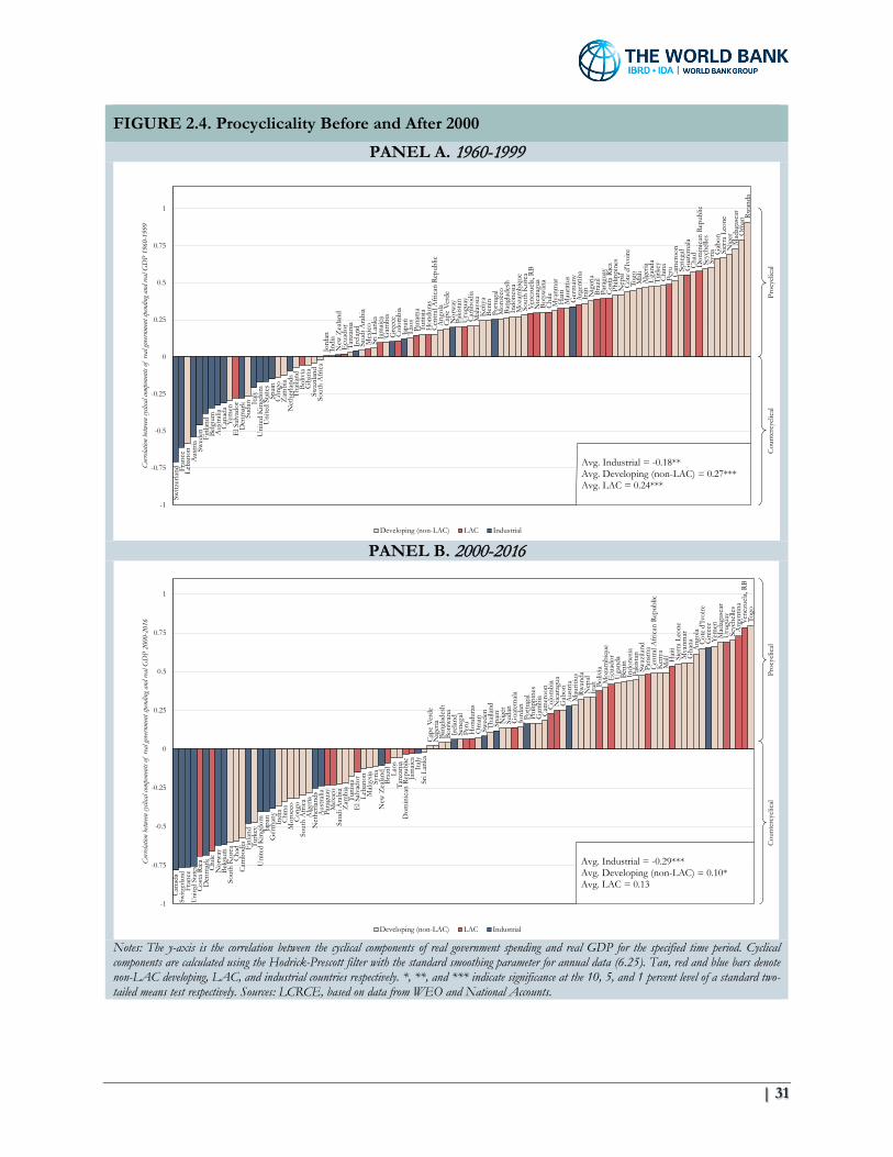
| 31
FIGURE 2.4. Procyclicality Before and After 2000
PANEL A. 1960-1999
PANEL B. 2000-2016
Notes: The y-axis is the correlation between the cyclical components of real government spending and real GDP for the specified time period. Cyclical components are calculated using the Hodrick-Prescott filter with the standard smoothing parameter for annual data (6.25). Tan, red and blue bars denote non-LAC developing, LAC, and industrial countries respectively. *, **, and *** indicate significance at the 10, 5, and 1 percent level of a standard two-tailed means test respectively. Sources: LCRCE, based on data from WEO and National Accounts.
Le
bano
n
Yem
en
Suda
n
Con
goZ
ambi
a
Thai
land
G
hana
Swaz
iland
Sout
h A
fric
aJo
rdan
Indi
a Ta
nzan
ia
Saud
i Ara
bia
Sr
i Lan
ka
Gam
bia
La
os
Tuni
sia
Cen
tral A
fric
an R
epub
licA
ngol
aC
ape
Verd
e
Paki
stan
C
ambo
dia
Mal
aysia
Ken
yaBe
nin
M
oroc
coBa
ngla
desh
Indo
nesia
Moz
ambi
que
Sout
h K
orea
Bo
tsw
ana
M
yanm
ar
Mau
ritiu
s
Iran Nig
eria
Ph
ilipp
ines
Nep
alC
ote
d'Iv
oire
Togo
Mal
iA
lger
iaU
gand
aTu
rkey
Chi
na
Cam
eroo
nSe
nega
l
Cha
d
Seyc
helle
sSy
ria Gab
onSi
erra
Leo
neN
iger
Mad
agas
car
Om
anRw
anda
E
l Sal
vado
r
Boliv
ia E
cuad
or
Mex
ico
Ja
mai
ca
Col
ombi
a
Pana
ma
H
ondu
ras
U
rugu
ay
Vene
zuel
a, RB
Nic
arag
ua
Chi
le
Hai
ti
Arg
entin
a
Braz
ilPa
ragu
ayC
osta
Ric
a
Peru
G
uate
mal
a
Dom
inic
an R
epub
lic
Switz
erla
nd Fran
ce
Aus
tria
Swed
en Finl
and
Belg
ium
Aus
tralia
Can
ada
D
enm
ark
It
aly
Uni
ted
Kin
gdom
Uni
ted
Stat
esSp
ain
N
ethe
rland
s N
ew Z
eala
nd
Irel
and
G
reec
e
Japa
n
Nor
way
Po
rtug
al
Ger
man
y
-1
-0.75
-0.5
-0.25
0
0.25
0.5
0.75
1
Corr
elatio
n be
tween
cycli
cal c
ompo
nent
s of
real g
overn
ment
spen
ding a
nd re
al G
DP
1960
-199
9
Developing (non-LAC) LAC Industrial
Avg. Industrial = -0.18**Avg. Developing (non-LAC) = 0.27***Avg. LAC = 0.24***
Proc
yclic
alC
ount
ercy
clic
al
So
uth
Kor
eaC
had
Cam
bodi
a
Turk
ey
Indi
aC
hina
Mor
occo
Con
goSo
uth
Afr
ica
Alg
eria
Sa
udi A
rabi
aZ
ambi
aTu
nisia
Le
bano
nM
alay
siaSy
ria
Laos
Tanz
ania
Sr
i Lan
kaC
ape
Verd
eN
iger
iaBa
ngla
desh
Bots
wan
a
Sene
gal
O
man
Th
aila
nd
Nig
erSu
dan
Jo
rdan
Ph
ilipp
ines
Gam
bia
Cam
eroo
n
Gab
on
Mau
ritiu
sRw
anda
Nep
alIr
an
Moz
ambi
que
U
gand
aBe
nin
Indo
nesia
Paki
stan
Swaz
iland
C
entra
l Afr
ican
Rep
ublic
Ken
yaM
ali
Si
erra
Leo
neM
yanm
arG
hana Ang
ola
Cot
e d'
Ivoi
re
Yem
enM
adag
asca
r
Seyc
helle
s
Togo
C
osta
Ric
a
Chi
le
Para
guay
Mex
ico
E
l Sal
vado
r
Braz
il
Dom
inic
an R
epub
licJa
mai
ca
Peru
Hon
dura
s
Gua
tem
ala
C
olom
bia
Nic
arag
ua
Boliv
ia
Ecu
ador
Pa
nam
a
Hai
ti
Uru
guay
A
rgen
tina
Vene
zuel
a, R
B
Can
ada
Switz
erla
ndFr
ance
Uni
ted
Stat
es
Den
mar
k
Nor
way
Belg
ium
Fi
nlan
d
Uni
ted
Kin
gdom
Japa
nG
erm
any
N
ethe
rland
sA
ustra
lia
New
Zea
land
It
aly
Ir
elan
d
Swed
en
Spai
n
Port
ugal
A
ustri
a
Gre
ece
-1
-0.75
-0.5
-0.25
0
0.25
0.5
0.75
1
Corr
elatio
n be
tween
cycli
cal c
ompo
nent
s of
real g
overn
ment
spen
ding
and
real
GD
P 20
00-2
016
Developing (non-LAC) LAC Industrial
Avg. Industrial = -0.29***Avg. Developing (non-LAC) = 0.10*Avg. LAC = 0.13
Proc
yclic
alC
ount
ercy
clic
al

32 | Leaning Against the Wind
FIGURE 2.5. The Shift towards Countercyclical Fiscal Policy–Before and After 2000
Notes: The y-axis and x-axis are the correlation between the cyclical components of real government spending and real GDP for the time period 2000-2016 and 1960-1999 respectively. Cyclical components are calculated using the Hodrick-Prescott filter with the standard smoothing parameter for annual data (6.25). Tan, red and blue bars denote non-LAC developing, LAC, and industrial countries respectively. Sources: LCRCE, based on data from WEO and National Accounts.
In this light, it is not surprising that over time many developing countries (including, of course, LAC countries) have been able to escape the fiscal procyclicality trap (see Frankel, Végh, and Vuletin, 2013). The two panels in Figure 2.4 visually show this phenomenon in a rather striking way. The 1960-2016 sample used in Figure 2.2 is divided into two sub-samples. The top panel shows the correlations between the cyclical components of government spending and real GDP for the period 1960-1999, whereas the bottom panel illustrates the same variable for the period 2000-2016.
Given the long sample, it is not surprising to see that the average correlation for 1960-1999 (0.24 for the case of LAC) in the top panel of Figure 2.4 is essentially the same as in Figure 2.2. The relevant comparison is with the bottom panel of Figure 2.4, which covers the period 2000-2016. The visual impression is already very telling as we can clearly see how a great deal of the tan and red mass on the RHS of the top panel has switched to the left in the bottom panel, indicating countries that were, on average, procyclical during the period 1960-1999 became countercyclical during the post-2000 period. In fact, the number of countercyclical LAC countries increased from 10 percent in the initial period (1960-1999) to 40 percent in the post-2000 period. This figure is the same as the one for other non-LAC developing countries.
As in Frankel, Végh, and Vuletin (2013), a convenient way of illustrating the countercyclical shift in the region is shown in Figure 2.5. The panel shows along the horizontal axis the correlation between the cyclical components of government spending and real GDP for the period 1960-1999 and along the vertical axis the correlations for the period 2000-2016. The plane is thus divided into four
India
S. Korea
Turkey
Syria
China
Thailand Philippines
Pakistan
Indonesia
ChileCosta Rica
Paraguay
El Salvador
Argentina
Peru
Mexico
JamaicaDom. Rep.Brazil
Ecuador
ColombiaGuatemala
Bolivia
Haiti
Panama
Uruguay
Venezuela, RB
USA
Denmark
France
Finland
Switzerland
Japan
Germany
UK
Belgium
Spain
Italy
Portugal
Greece
-1
-0.8
-0.6
-0.4
-0.2
0
0.2
0.4
0.6
0.8
1
-1 -0.8 -0.6 -0.4 -0.2 0 0.2 0.4 0.6 0.8 1
Corr(
G,G
DP)
200
0-20
16
Corr(G,GDP) 1960-1999
Developing (non-LAC) LAC Industrial
Back to procyclicality Still procyclical
Established countercyclical New countercyclical

| 33
FIGURE 2.6. Procyclicality and Institutional Quality
Notes: The x-axis shows the Institutional Quality Index which is the average of the following indices: bureaucratic quality, corruption, investment profile, and law and order. The y-axis is the correlation between the cyclical components of real government spending and real GDP for the time period 1960-2016. Cyclical components are calculated using the Hodrick-Prescott filter with the standard smoothing parameter for annual data (6.25). *, **, and *** indicate significance at the 10, 5, and 1 percent level for the regression slope respectively. Sources: LCRCE, based on data from ICRG, WEO, and National Accounts.
quadrants: the lower LHS quadrant (labeled “Established countercyclical”) denotes countries, such as the USA and the UK, that have always been countercyclical. The lower RHS quadrant (labeled “New countercyclical”) indicates countries, such as Chile and Mexico, that switched from being procyclical in the earlier period to countercyclical in the most recent period. The upper RHS quadrant (labeled “Still procyclical”) indicates countries, such as Nicaragua that continue to be procyclical. Finally, the upper-LHS quadrant (labeled “Back to procyclicality”) shows the handful of countries that have, unfortunately, switched from being countercyclical during the first period to being procyclical during the second period.
What lies behind the process of becoming countercyclical? In other words, what explains the difference between a country (like Chile) that has been able to become countercyclical and a country that has not? The question of what enables a country to become countercyclical is a complex one and therefore there will not be a single “silver bullet” that will transform a country that has spent, possibly, decades trapped in the procyclical camp into a countercyclical country. Rather, we should expect a combination of improvements in the budgetary processes, in transparency of bidding mechanisms, and, more generally, in the efficiency of the overall quality of public institutions to slowly, but surely, contribute to the overall process of becoming countercyclical.
Figure 2.6 illustrates, from an empirical point of view, the critical role that institutional quality plays in allowing countries to become countercyclical. To this effect we have taken a simple average of four indices of institutional quality constructed by the World Bank (Bureaucratic Quality, Corruption,
Switzerland
Germany
USA
UK
Japan
Chile
Italy
Greece
Costa Rica
China
Mexico
Turkey
Argentina
Brazil
Colombia
Peru
El Salvador
Bolivia
Venezuela, RB
Haiti
-1
-0.8
-0.6
-0.4
-0.2
0
0.2
0.4
0.6
0.8
1
0.1 0.2 0.3 0.4 0.5 0.6 0.7 0.8 0.9 1
Gov
ernme
nt S
pend
ing P
rocyc
licali
ty 19
60-2
016
Institutional Quality Index 1984-2016
Regression line:Corr(G, GDP) = 0.7 - 0.9*** IQ

34 | Leaning Against the Wind
Investment Profile, and Law and Order), normalized between 0 and 1.16 This average is shown along the horizontal axis. The vertical axis shows the usual fiscal spending procyclicality index, measured by the cyclical components of government spending and GDP. There is a highly significant relationship indicating that increases in institutional quality are associated with a reduction in procyclicality or an increase in countercyclicality.17
In addition to the overall improvement in the quality of fiscal institutions and the rule of law highlighted in Figure 2.6, there are some specific features worth mentioning that have contributed to several countries becoming countercyclical in LAC. In the case of Chile, a critical element was the implementation in the year 2001 of a fiscal rule that required the central government to achieve a structural surplus of 1 percent of GDP, which was eventually reduced to 0.18 The structural balance is computed by adjusting the actual fiscal balance for the deviation of actual tax revenues from trend growth and for deviations of copper prices from their long-term values. It is important to notice that, by construction, a structural budget rule that requires the government to achieve a zero structural balance will ensure that the government saves temporary windfalls in good times and dis-saves in bad times. In other words, the economy will show actual surpluses in good times and actual deficits in bad times.19
An important feature of these adjustments in Chile is that they are carried out by an independent group of experts, which ensures an objective evaluation of the cyclical component of both tax revenues and copper prices. While the process will never be perfect, the presence of independent experts ensures that it will not be subject to political manipulation.
As Figure 2.7 makes clear, even a structural balance budget rule is no panacea and Chile itself broke its own rule during the Global Financial Crisis in 2009 when it embarked in a very aggressive countercyclical fiscal policy that took the structural fiscal deficit to 3.1 percent of GDP. Furthermore, according to IMF-WEO estimates, the projected structural deficit for 2017 is 1.9 percent of GDP, with the objective of gradually reducing it to 0.8 percent of GDP at the end of this decade. However,
16 The IQ index ranges between 0 and 1 where higher values indicate higher institutional quality. The index equally weighs four variables from the International Country Risk Guide. Investment Profile is an investment risk measure capturing contract viability and expropriation, profits repatriation, and payment delays; Corruption is an assessment of the corruption within the political system; Law and Order captures the strength and impartiality of the legal system and the popular observance of the law; Bureaucratic Quality measures the presence of drastic changes in policy or interruptions in government services. For a more detailed explanation see Frankel, Végh, and Vuletin (2013). 17 Needless to say, a more formal analysis would control for the possible endogeneity of institutions and other determinants of fiscal procyclicality. By using instrumental variables, Frankel, Végh, and Vuletin (2013) show that the results are robust to using instrumental variables so that causality runs from stronger institutions to less procyclical or more countercyclical fiscal policy. Carneiro and Odawara (2015) obtain similar findings for the Eastern Caribbean countries following the same methodology. 18 The target of 1 percent reflected the need to repay Central Bank debt associated with the bailout of private banks in the 1980s (see Frankel, 2011, for details). As this debt was paid off, the structural target was reduced to 0.5 percent in 2008 and 0 percent in 2009. 19 Contrary, however, to what is commonly claimed, Chile’s structural balanced rule is not a countercyclical rule per se. For that to be true, the rule should require a structural deficit in bad times, which would be compensated by a structural surplus in good times.

| 35
FIGURE 2.7. Chile’s Fiscal Rule
Notes: Targeted structural balances are taken from the ‘Politica de Balance Estructural’ reports from DIPRES. Sources: ‘Banco Central de Chile’ and ‘Direccion de Presupuestos - Gobierno de Chile’.
even if it is not a silver bullet, a structural fiscal rule focuses the public policy discussion and the tough fiscal debates on the right track, by calling attention to the fact that, given the highly volatile business cycles that our region experiences, the best indicators of fiscal health (or lack thereof) are structural balances and not actual balances.20
Colombia is another example of a LAC country that passed a law on July 5, 2011, requiring the government to meet certain structural fiscal targets. The law, which started being implemented in 2012, adjusts the actual fiscal balance for oil revenues and the output gap, and calls for reaching a structural deficit of no more than 1 percent of GDP in the year 2022, with a target of less than 2.3 percent of GDP by 2014 and 1.9 percent by 2018.21
Needless to say, structural budget rules are not the only type of rules that have been used. Table 2.1, based on Schaechter et. al (2012), reviews different types of rules with their pros and cons. Even though structural budget rules are in theory the best, in practice the computation of structural budgets, particularly in LAC countries where the business cycle is highly volatile and subject to a myriad of external, domestic, and natural shocks is an enormous challenge. Still, simple structural adjustments would give policymakers a better picture than no adjustments at all.22
20 Casual empiricism is very clear on this. In countries such as Chile and Colombia, which have structural fiscal rules, even discussions in the financial press focus on those important concepts and hence put fiscal discussions in the proper context. This is not the case in other countries where structural balances are rarely mentioned in the public arena which allows, for example, the fiscal authority to claim excellent fiscal performances in good times when, in reality, fiscal balances would look much weaker if adjusted by the cycle (the “all that glitters may not be gold” syndrome highlighted by IDB (2008)). 21 The law can be found in http://www.secretariasenado.gov.co/senado/basedoc/ley_1473_2011.html. See also IMF (2014). 22 The simplest structural adjustment, which is widely used, is the so-called 0-1 method. This methodology assumes an elasticity of revenues with respect to real GDP of 1 and adjusts accordingly while leaving expenditures intact. For detailed
-6
-4
-2
0
2
4
6
8
10
2001 2002 2003 2004 2005 2006 2007 2008 2009 2010 2011 2012 2013 2014 2015
perce
nt of
GD
P
Fiscal Balance Structural Balance Targeted Structural Balance

36 | Leaning Against the Wind
TABLE 2.1. Fiscal Rules
Sources: Table 1 from Schaechter et. al. (2012)
For example, a rule that simply requires a balanced budget at all times is probably the worst rule of all. If followed, it would ensure “perfect procyclicality” in the sense that revenue increases (reductions) would be exactly matched by spending increases (reductions) to ensure a zero balance at all times. In fact, most states in the United States have balanced budget rules, which has ensured that almost all U.S. states are procyclical (even though the federal government is not). This is clearly illustrated in Figure 2.8, which shows the correlation between the cyclical components of provincial/state GDP in Argentina and the U.S. with the corresponding levels of spending. While the fact that all, except one, Argentine provinces are procyclical with a mean correlation of 0.46 was to be expected, the fact that the same is true of U.S. states (with essentially the same mean correlation) is quite shocking and mostly due to the unwise choice of having balanced budget rules that violate any sound theoretical principle of optimal fiscal policy.23
Another two institutional features that are of help are, first, commodities funds such as the old Chilean Copper Stabilization Fund (FEC), which in 2007 became the Economic and Social Stabilization Fund (FEES). The main purpose of this fund is to prevent government spending from being greatly affected
analyses of cyclical adjustments, see, for example, Escolano (2010), Fedelino, Ivanova, and Horton (2009), and Girouard and Andre (2005). 23 Not surprisingly in light of the Argentine experience, Colombia imposed in 1997 and 2000 fiscal constraints at the sub-national level that limit the level of indebtedness of sub-national governments; see IMF (2014) for details.
Type of rule Pros Cons
- Direct link to debt sustainability - No clear operational guidance in the short run as policy impact on debt ratio is not immediate and limited
- Easy to communicate and monitor - No economic stabilization feature (can be pro-cyclical) - Rule could be met via temporary measures (e.g., below-the-line transactions) - Debt could be affected by developments outside the control of the government
- Clear operational guidance - No economic stabilization feature (can be pro-cyclical)
- Close link to debt sustainability - Headline balance could be affected by developments outside the control of the government (e.g., a major economic downturn)
- Easy to communicate and monitor
- Relatively clear operational guidance - Correction for cycle is complicated, especially for countries undergoing structural changes
- Close link to debt sustainability - Need to pre-define one-off and temporary factors to avoid their discretionary use
- Economic stabilization function (i.e., accounts for economic shocks) - Complexity makes it more difficult to communicate and monitor
- Allows to account for other one-off and temporary factors
- Clear operational guidance - Not directly linked to debt sustainability since no constraint on revenue side
- Allows for economic stabilization - Could lead to unwanted changes in the distribution of spending if, to meet the ceiling, shift to spending categories occurs that are not covered by the rule
- Steers the size of government - Relatively easy to communicate and monitor
- Steers the size of government - Not directly linked to debt sustainability since no constraint on expenditure side (except rules constraining use of windfall revenue)
- Can improve revenue policy and administration - No economic stabilization feature (can be pro-cyclical) - Can prevent pro-cyclical spending (rules constraining use of windfall revenue)
Debt rule
Budget balance rule
Structural budget balance
rule
Expenditure rule
Revenue rule

| 37
FIGURE 2.8. Procyclicality at the Sub-National Level: Argentina and the U.S.
PANEL A. Argentina
PANEL B. U.S.
Notes: *, **, and *** indicate significance at the 10, 5, and 1 percent level of a standard two-tailed means test respectively. Sample periods for Panel A and B are 1961-2006 and 1963-2005, respectively. Sources: Argentine National and Provincial Data and U.S. Census Bureau
by the vagaries of the world economy (including copper and tax revenues) by saving in good times and using these funds as needed in bad times. The second institutional feature – very common in industrial countries – are automatic stabilizers. These are government expenditures, such as unemployment insurance and food stamps programs in the United States, which will automatically increase in bad times (as unemployment and poverty experience a cyclical increase) and fall in good times. Such programs make an essential contribution to countercyclical fiscal policy.
LAC’s Switch to Countercyclical Policy since the Global Financial Crisis While LAC countries share many similarities with the developing world as a whole, they also present some special characteristics that are worth mentioning. The goal of this section is thus to apply to LAC countries the fiscal analysis carried out above for all developing countries in order to draw specific policy prescriptions for the region. In addition, and unlike in the previous section, we will
Neu
quen
San
Luis
Tier
ra d
el F
uego
Sant
a Fe
La P
ampa
Cor
rient
esSa
nta
Cru
zLa
Rio
jaFo
rmos
aC
haco
Cat
amar
caRi
o N
egro
Men
doza
Chu
but
Misi
ones
Ent
re R
ios
Salta
Sant
iago
del
Est
ero
C.A
.B.A
.Ju
juy
Cor
doba
Tucu
man
San
Juan
Buen
os A
ires
Arg
entin
a
-0.4
-0.2
0
0.2
0.4
0.6
0.8
1
Corr
elatio
n be
tween
cycli
cal c
ompo
nent
s of
real s
pend
ing a
nd re
al ou
tput
19
61-2
006
Avg. Provinces = 0.46***
New
Ham
pshi
re
Nev
ada
Uta
hTe
xas
New
Mex
ico
Mai
neC
alifo
rnia
Nor
th D
akot
aA
rizon
aW
ashi
ngto
nM
assa
chus
etts
Con
nect
icut
Loui
siana
New
Jers
eySo
uth
Car
olin
aM
onta
naO
klah
oma
Mar
ylan
dG
eorg
iaR
hode
Isla
ndFl
orid
aW
yom
ing
Mic
higa
nV
irgin
iaN
ew Y
ork
Del
awar
eVe
rmon
tN
orth
Car
olin
aK
ansa
sK
entu
cky
Haw
aii
Illin
ois
Ohi
oSo
uth
Dak
ota
Ala
bam
aA
lask
aC
olor
ado
Min
neso
taW
iscon
sinM
issou
riIn
dian
aO
rego
nW
est V
irgin
iaTe
nnes
see
Neb
rask
aPe
nnsy
lvan
iaM
ississ
ippi
Ark
ansa
sId
aho
Iow
a
Uni
ted
Stat
es
-1
-0.75
-0.5
-0.25
0
0.25
0.5
0.75
1
Corr
elatio
n be
tween
cycli
cal c
ompo
nent
s of
real s
pend
ing a
nd re
al ou
tput
19
63-2
005
Avg. States = 0.43***
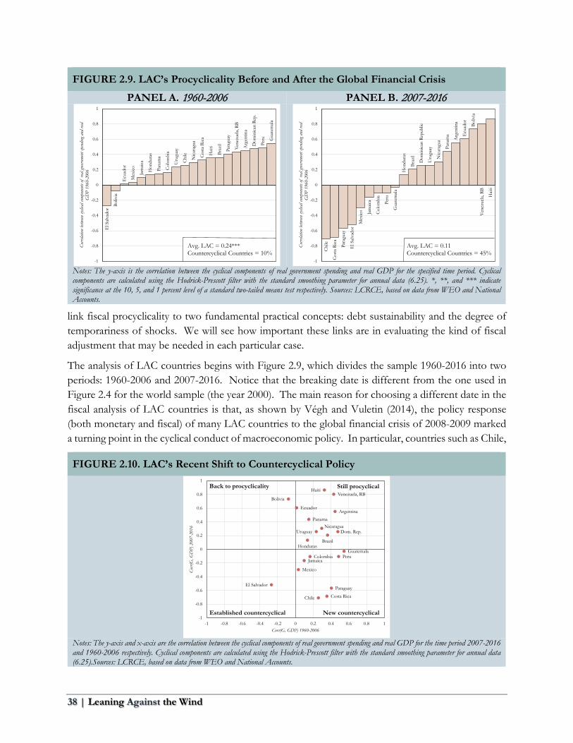
38 | Leaning Against the Wind
FIGURE 2.9. LAC’s Procyclicality Before and After the Global Financial Crisis
PANEL A. 1960-2006 PANEL B. 2007-2016
Notes: The y-axis is the correlation between the cyclical components of real government spending and real GDP for the specified time period. Cyclical components are calculated using the Hodrick-Prescott filter with the standard smoothing parameter for annual data (6.25). *, **, and *** indicate significance at the 10, 5, and 1 percent level of a standard two-tailed means test respectively. Sources: LCRCE, based on data from WEO and National Accounts.
link fiscal procyclicality to two fundamental practical concepts: debt sustainability and the degree of temporariness of shocks. We will see how important these links are in evaluating the kind of fiscal adjustment that may be needed in each particular case.
The analysis of LAC countries begins with Figure 2.9, which divides the sample 1960-2016 into two periods: 1960-2006 and 2007-2016. Notice that the breaking date is different from the one used in Figure 2.4 for the world sample (the year 2000). The main reason for choosing a different date in the fiscal analysis of LAC countries is that, as shown by Végh and Vuletin (2014), the policy response (both monetary and fiscal) of many LAC countries to the global financial crisis of 2008-2009 marked a turning point in the cyclical conduct of macroeconomic policy. In particular, countries such as Chile,
FIGURE 2.10. LAC’s Recent Shift to Countercyclical Policy
Notes: The y-axis and x-axis are the correlation between the cyclical components of real government spending and real GDP for the time period 2007-2016 and 1960-2006 respectively. Cyclical components are calculated using the Hodrick-Prescott filter with the standard smoothing parameter for annual data (6.25).Sources: LCRCE, based on data from WEO and National Accounts.
El S
alva
dor Bo
livia
Ecu
ador
Mex
ico
Jam
aica
Hon
dura
s
Pana
ma
Col
ombi
a
Uru
guay
Chi
le
Nic
arag
ua
Cos
ta R
ica
Hai
ti
Braz
il
Para
guay
Vene
zuel
a, RB
Arg
entin
a
Dom
inic
an R
ep.
Peru G
uate
mal
a
-1
-0.8
-0.6
-0.4
-0.2
0
0.2
0.4
0.6
0.8
1
Corr
elatio
n be
tween
cycli
cal c
ompo
nent
s of
real g
overn
ment
spen
ding a
nd re
al G
DP
1960
-200
6
Avg. LAC = 0.24***Countercyclical Countries = 10% C
hile
Cos
ta R
ica
Para
guay
El S
alva
dor
Mex
ico Jam
aica
Col
ombi
a
Peru
Gua
tem
ala
Hon
dura
s
Braz
il
Dom
inic
an R
epub
lic
Uru
guay
Nic
arag
ua
Pana
ma
Arg
entin
a
Ecu
ador Bo
livia
-1
-0.8
-0.6
-0.4
-0.2
0
0.2
0.4
0.6
0.8
1
Ven
ezue
la, R
B
Hai
ti
Corr
elatio
n be
tween
cycli
cal c
ompo
nent
s of
real g
overn
ment
spen
ding a
nd re
al G
DP
1960
-200
6
Avg. LAC = 0.11Countercyclical Countries = 45%
Chile Costa Rica
ParaguayEl Salvador
Argentina
Peru
Mexico
Honduras
Jamaica
Dom. Rep.
Brazil
Ecuador
ColombiaGuatemala
Bolivia
Haiti
PanamaNicaragua
Uruguay
Venezuela, RB
-1
-0.8
-0.6
-0.4
-0.2
0
0.2
0.4
0.6
0.8
1
-1 -0.8 -0.6 -0.4 -0.2 0 0.2 0.4 0.6 0.8 1
Corr(
G, G
DP)
200
7-20
16
Corr(G, GDP) 1960-2006
Back to procyclicality Still procyclical
Established countercyclical New countercyclical

| 39
FIGURE 2.11. Procyclicality and Institutional Quality in LAC
Notes: The x-axis shows the Institutional Quality Index which is the average of the following indices: bureaucratic quality, corruption, investment profile, and law and order. The y-axis is the correlation between the cyclical components of real government spending and real GDP for the time period 2007-2016. Cyclical components are calculated using the Hodrick-Prescott filter with the standard smoothing parameter for annual data (6.25). *, **, and *** indicate significance at the 10, 5, and 1 percent level for the regression slope respectively. Sources: LCRCE, based on data from ICRG, WEO, and National Accounts.
Mexico, Brazil, and Peru showed a countercyclical fiscal response in at least one fiscal dimension (spending, taxation or both). Chile, in particular, implemented one of the largest stimulus programs in the world (with a package worth 2.8 percent of GDP, comparable to the one passed by the United States Congress in early 2009).24 Another reason for choosing the year 2007 as the turnaround date is that casual empiricism suggests that fiscal macroeconomic management has improved in many countries since then.
Figure 2.9 shows in quite a dramatic fashion the shift to countercyclical fiscal policy discussed above. During the period 1960-2006, only two out of 20 countries (i.e., 10 percent) were countercyclical, with an average correlation of 0.24 (statistically significant at the 1 percent level). In sharp contrast, during the 2007-2016 period, eight countries shifted to countercyclical fiscal policy, thus increasing the ratio of countercyclical countries from 10 percent to 45 percent, a remarkable turnaround for the region. Further, notice that the eight countries that became countercyclical include countries from both sub-regions, namely SA (Chile, Paraguay, Colombia, and Peru) and MCC (Costa Rica, Mexico, Jamaica, and Guatemala). Finally, it is also worth mentioning that the average correlation is still positive (0.10) but no longer significantly different from zero. In sum, while we should definitely not declare victory since many countries continue to behave procyclically and, as we shall see below, the problem of debt sustainability is, once again, raising its ugly head, we can certainly celebrate the fact that the region appears to have begun to finally break the shackles of the procyclicality trap.
Like before, the shift to countercyclical fiscal policy can be illustrated by means of the scatter plot in Figure 2.10. The scatter plot shows the great progress that has been made (notice all the countries in the “New countercyclical” quadrant) at the same time that it calls attention to the work that remains
24 Incidentally, Chile implemented an equally aggressive countercyclical monetary policy, reducing the monetary policy rate by 775 basis points (from 8.25 percent in December 2008 to 0.5 percent in July 2009).
ChileCosta RicaParaguay
El Salvador GuatemalaColombia
MexicoPeru Jamaica
HondurasBrazil
UruguayDom. Rep.
ArgentinaPanama
Ecuador
BoliviaNicaraguaVenezuela, RB
Haiti
-1
-0.8
-0.6
-0.4
-0.2
0
0.2
0.4
0.6
0.8
1
0.1 0.2 0.3 0.4 0.5 0.6 0.7 0.8 0.9
Gov
ernme
nt S
pend
ing P
rocyc
licali
ty 20
07-2
016
Institutional Quality Index 2007-2016
Regression line:Corr(G, GDP) = 1.1 - 2.2** IQ

40 | Leaning Against the Wind
to be done (notice all the countries in the “Still procyclical” quadrant). The share of countries that became countercyclical is 44 percent.25
Figure 2.11 shows the regression line linking the correlation between government spending and institutional quality for the period 2007-2016. The relation is highly significant, thus highlighting the importance of the improvement in the quality of the regional institutions on countries’ ability to escape the procyclicality trap.
Countercyclicality and Procyclicality in LAC: Country Examples The analysis of procyclicality and the switch to countercyclicality can now be applied to some of the main countries in the region. While space precludes us from doing this detailed analysis for each country in the region, a few examples should suffice to show how helpful the analysis can be in understanding, assessing, and eventually correcting (as needed) the conduct of fiscal policy.
Just as a summary that will guide the analysis, Table 2.2 lists 10 countries in the region: six that have become countercyclical (Chile, Colombia, Guatemala, Mexico, Paraguay, and Peru) and four that are still procyclical (Bolivia, Nicaragua, Panama, and Uruguay).
The six panels in Figure 2.12 show two lines for each of the countries that became countercyclical: the red line is the cyclical component of real government spending during the period 2007-2016, whereas the blue line captures the cyclical component of real GDP during the same period. In other words, when the blue line is above 0, it indicates a positive output gap (the economy is in a boom). When the blue line is below 0, the output gap is negative and the economy is in the midst of a recession.
As an example, let us take a close look at the case of Chile (Panel A). The countercyclical behavior of government spending during the Global Financial Crisis is particularly striking. With a negative output
TABLE 2.2. Selected LAC Countries
Notes: Improvements have a positive value when a country is more countercyclical in 2007-2016 than in 1960-2006. Sources: LCRCE based on data from WEO and National Accounts.
25 Using a very different methodology, Adler and Magud (2015) find that fiscal performance in Latin American has been more prudent during the recent boom (which ends in 2012 in their sample), with a median increase in public savings of 2.5 percent of GDP, compared with 1.3 percent in previous episodes. This is, in principle, consistent with our shift to countercyclicality story.
1960-2006 2007-2016 ImprovementChile 0.23 -0.63 0.86Colombia 0.18 -0.35 0.53Guatemala 0.54 -0.42 0.96Mexico 0.03 -0.17 0.2Paraguay 0.40 -0.56 0.97Peru 0.48 -0.09 0.57Bolivia -0.08 0.76 -0.84Nicaragua 0.29 0.77 -0.48Panama 0.15 0.48 -0.33Uruguay 0.23 0.26 -0.02
Still Procyclical
New Countercyclical

| 41
FIGURE 2.12. Countercyclical Selected LAC Countries
PANEL A. Chile PANEL B. Colombia
PANEL C. Guatemala PANEL D. Mexico
PANEL E. Paraguay PANEL F. Peru
Notes: Cyclical components are calculated using the Hodrick-Prescott filter with the standard smoothing parameter for annual data (6.25). Sources: LCRCE, based on data from WEO and National Accounts.
-6
-4
-2
0
2
4
6
8
2007 2008 2009 2010 2011 2012 2013 2014 2015 2016
perce
nt of
tren
d
Expenditure Cyclical Component GDP Cyclical Component
-6
-5
-4
-3
-2
-1
0
1
2
3
4
5
2007 2008 2009 2010 2011 2012 2013 2014 2015 2016
perce
nt of
tren
d
Expenditure Cyclical Component GDP Cyclical Component
-5
-4
-3
-2
-1
0
1
2
3
4
2007 2008 2009 2010 2011 2012 2013 2014 2015 2016
perce
nt of
tren
d
Expenditure Cyclical Component GDP Cyclical Component
-5
-4
-3
-2
-1
0
1
2
3
4
5
2007 2008 2009 2010 2011 2012 2013 2014 2015 2016
perce
nt of
tren
d
Expenditure Cyclical Component GDP Cyclical Component
-6
-4
-2
0
2
4
6
2007 2008 2009 2010 2011 2012 2013 2014 2015 2016
perce
nt of
tren
d
Expenditure Cyclical Component GDP Cyclical Component
-4
-3
-2
-1
0
1
2
3
4
2007 2008 2009 2010 2011 2012 2013 2014 2015 2016
perce
nt of
tren
d
Expenditure Cyclical Component GDP Cyclical Component
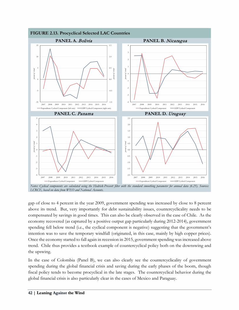
42 | Leaning Against the Wind
FIGURE 2.13. Procyclical Selected LAC Countries
PANEL A. Bolivia PANEL B. Nicaragua
PANEL C. Panama PANEL D. Uruguay
Notes: Cyclical components are calculated using the Hodrick-Prescott filter with the standard smoothing parameter for annual data (6.25). Sources: LCRCE, based on data from WEO and National Accounts.
gap of close to 4 percent in the year 2009, government spending was increased by close to 8 percent above its trend. But, very importantly for debt sustainability issues, countercyclicality needs to be compensated by savings in good times. This can also be clearly observed in the case of Chile. As the economy recovered (as captured by a positive output gap particularly during 2012-2014), government spending fell below trend (i.e., the cyclical component is negative) suggesting that the government’s intention was to save the temporary windfall (originated, in this case, mainly by high copper prices). Once the economy started to fall again in recession in 2015, government spending was increased above trend. Chile thus provides a textbook example of countercyclical policy both on the downswing and the upswing.
In the case of Colombia (Panel B), we can also clearly see the countercyclicality of government spending during the global financial crisis and saving during the early phases of the boom, though fiscal policy tends to become procyclical in the late stages. The countercyclical behavior during the global financial crisis is also particularly clear in the cases of Mexico and Paraguay.
-1.0
-0.5
0.0
0.5
1.0
1.5
-10
-5
0
5
10
15
2007 2008 2009 2010 2011 2012 2013 2014 2015 2016
perce
nt of
tren
d
perce
nt of
tren
d
Expenditure Cyclical Component (left axis) GDP Cyclical Component (right axis)
-4
-3
-2
-1
0
1
2
3
4
2007 2008 2009 2010 2011 2012 2013 2014 2015 2016
perce
nt of
tren
d
Expenditure Cyclical Component GDP Cyclical Component
-4
-3
-2
-1
0
1
2
3
4
5
2007 2008 2009 2010 2011 2012 2013 2014 2015 2016
perce
nt of
tren
d
Expenditure Cyclical Component GDP Cyclical Component
-2.0
-1.5
-1.0
-0.5
0.0
0.5
1.0
1.5
2.0
2.5
2007 2008 2009 2010 2011 2012 2013 2014 2015 2016
perce
nt of
tren
d
Expenditure Cyclical Component GDP Cyclical Component
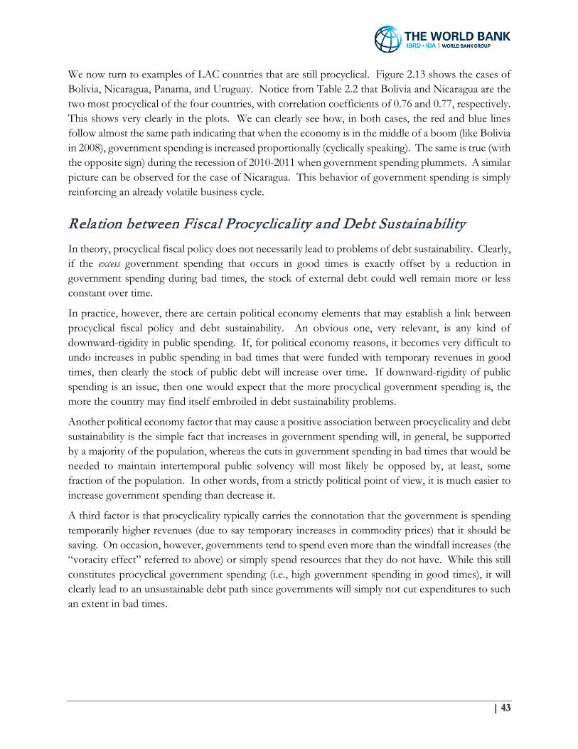
| 43
We now turn to examples of LAC countries that are still procyclical. Figure 2.13 shows the cases of Bolivia, Nicaragua, Panama, and Uruguay. Notice from Table 2.2 that Bolivia and Nicaragua are the two most procyclical of the four countries, with correlation coefficients of 0.76 and 0.77, respectively. This shows very clearly in the plots. We can clearly see how, in both cases, the red and blue lines follow almost the same path indicating that when the economy is in the middle of a boom (like Bolivia in 2008), government spending is increased proportionally (cyclically speaking). The same is true (with the opposite sign) during the recession of 2010-2011 when government spending plummets. A similar picture can be observed for the case of Nicaragua. This behavior of government spending is simply reinforcing an already volatile business cycle.
Relation between Fiscal Procyclicality and Debt Sustainability In theory, procyclical fiscal policy does not necessarily lead to problems of debt sustainability. Clearly, if the excess government spending that occurs in good times is exactly offset by a reduction in government spending during bad times, the stock of external debt could well remain more or less constant over time.
In practice, however, there are certain political economy elements that may establish a link between procyclical fiscal policy and debt sustainability. An obvious one, very relevant, is any kind of downward-rigidity in public spending. If, for political economy reasons, it becomes very difficult to undo increases in public spending in bad times that were funded with temporary revenues in good times, then clearly the stock of public debt will increase over time. If downward-rigidity of public spending is an issue, then one would expect that the more procyclical government spending is, the more the country may find itself embroiled in debt sustainability problems.
Another political economy factor that may cause a positive association between procyclicality and debt sustainability is the simple fact that increases in government spending will, in general, be supported by a majority of the population, whereas the cuts in government spending in bad times that would be needed to maintain intertemporal public solvency will most likely be opposed by, at least, some fraction of the population. In other words, from a strictly political point of view, it is much easier to increase government spending than decrease it.
A third factor is that procyclicality typically carries the connotation that the government is spending temporarily higher revenues (due to say temporary increases in commodity prices) that it should be saving. On occasion, however, governments tend to spend even more than the windfall increases (the “voracity effect” referred to above) or simply spend resources that they do not have. While this still constitutes procyclical government spending (i.e., high government spending in good times), it will clearly lead to an unsustainable debt path since governments will simply not cut expenditures to such an extent in bad times.

44 | Leaning Against the Wind
FIGURE 2.14. Procyclicality and Long-Term Credit Ratings
Notes: The x-axis is the long-term credit rating as reported by Fitch. The y-axis is the correlation between the cyclical components of real government spending and real GDP for the time period 2007-2016. Cyclical components are calculated using the Hodrick-Prescott filter with the standard smoothing parameter for annual data (6.25). *, **, and *** indicate significance at the 10, 5, and 1 percent level for the regression slope respectively. Sources: Fitch and LCRCE, based on data from WEO and National Accounts.
Based on these arguments, one would also suspect that the more procyclical a country is, the more unsustainable the debt will become.26 While a full analysis of this issue is clearly beyond the scope of this report (and would require controlling for many other factors that may lead to increases in debt), Figure 2.14 presents suggestive evidence of the link between procyclicality and debt sustainability. Along the horizontal axis, we use Fitch Credit Ratings (2016 review) that capture the risk premium associated with each country. The vertical axis shows the correlation between the cyclical components of government spending and real GDP during the period 2007-2016. Each point in the plot represents one of the 16 countries that carry a Fitch rating. We can see a highly significant negative relationship between the degree of procyclicality and the quality of the credit rating: the more procyclical the country, the worse its credit rating.27
26 See Alberola et. al. 2006. 27 Needless to say, more work would be needed to formally establish this chain of causality.
Venezuela, RB
Argentina
El Salvador
Bolivia
Brazil
Costa Rica
Uruguay
Colombia
Mexico
Chile
Ecuador
Nicaragua
Dominican Republic
Guatemala
Peru
Paraguay
0
0.1
0.2
0.3
0.4
0.5
0.6
0.7
0.8
0.9
1
-1
-0.8
-0.6
-0.4
-0.2
0
0.2
0.4
0.6
0.8
1
CCC CCC+ B- B B+ BB- BB BB+ BBB- BBB BBB+ A- A A+
Exp
endit
ure P
rocyc
licali
ty 20
07-2
016
Fitch long-term credit rating
Regression line:Corr(G, GDP) = -0.1*** Rating - 1.2
Investment GradeHigh Credit Risk and AboveSubstantial Credit Risk

| 45
Examples of Procyclicality and Increasing Debt: Brazil and Ecuador To provide some concrete examples of the relation between procyclicality and debt, Figure 2.15 illustrates the cases of Brazil and Ecuador. 28 In each case, the LHS panel shows the cyclical components of real government spending and real GDP, while the RHS panel shows the indices of real expenditures, real primary expenditures, real revenues, and the cumulative increases in net debt since 2007.
FIGURE 2.15. Procyclical Selected LAC Countries
PANEL A. Brazil Cyclical Components
PANEL B. Brazil Revenue, Expenditure, and Net Debt
Increase
PANEL C. Ecuador
Cyclical Components
PANEL D. Ecuador Revenue, Expenditure, and Net Debt
Increase
Notes: Cyclical components are calculated using the Hodrick-Prescott filter with the standard smoothing parameter for annual data (6.25). Real revenue, real expenditure, and real primary expenditure are indexed (2007 = 100). Net Debt Increase since 2007 is the sum of real fiscal deficits since 2007 as a share of the 2007 real GDP. Sources: LCRCE, based on data from WEO and National Accounts.
28 Just as a reminder, the correlations between the cyclical components of government spending and real GDP for Brazil and Ecuador during 2007-2016 are 0.21 and 0.61, respectively.
-4
-3
-2
-1
0
1
2
3
2007 2008 2009 2010 2011 2012 2013 2014 2015 2016
perce
nt of
tren
d
Expenditure Cyclical Component GDP Cyclical Component
0
5
10
15
20
25
95
100
105
110
115
120
125
130
135
2007 2008 2009 2010 2011 2012 2013 2014 2015 2016 2017
shar
e of
2007
GD
P
Inde
x (2
007
= 1
00)
Net Debt Increase since 2007 (right axis) Real Revenue Index
Real Expenditure Index Real Primary Expenditure Index
-4.0
-3.0
-2.0
-1.0
0.0
1.0
2.0
3.0
4.0
-15
-10
-5
0
5
10
15
2007 2008 2009 2010 2011 2012 2013 2014 2015 2016
perce
nt of
tren
d
Expenditure Cyclical Component (left axis) GDP Cyclical Component (right axis)
0
5
10
15
20
25
30
35
90
110
130
150
170
190
210
230
250
270
290
2007 2008 2009 2010 2011 2012 2013 2014 2015 2016 2017
shar
e of
2007
GD
P
Inde
x (2
007
= 1
00)
Net Debt Increase since 2007 (right axis) Real Revenue Index
Real Expenditure Index Real Primary Expenditure Index

46 | Leaning Against the Wind
In the case of Brazil, we can see from the LHS panel that Brazil was highly procyclical during the Global Financial Crisis, with a sharp fall in spending in the midst of the recession. Even though reinforcing the recession with a reduction in government spending is far from ideal, the fact that spending is falling roughly in tandem with revenues precludes debt unsustainability issues from taking hold. And Brazil, in fact, saved some of the commodities windfall during 2002-2014. But once the recession started, government spending turned countercyclical but was accompanied by a very sharp cyclical fall in revenues. Having not saved enough, this fiscal behavior was bound to generate debt problems. Furthermore, the Central Bank of Brazil raised the policy rate (SELIC) quite sharply from about 10 percent at the beginning of 2014 to over 14 percent by mid-2015 to defend the domestic currency and combat inflation, which naturally also increased the interest rate on the public debt. The combination of these factors has contributed to a large rise in debt.29
For the case of Ecuador, the procyclicality of government spending is quite evident from the LHS panel, with cyclical spending falling during the Global Financial Crisis and increasing during the commodity boom of 2012-2014. The RHS panel, however, clearly shows that government spending is higher than revenues both in the boom and in the bust, which will naturally result in large increases in the stock of net debt. This case thus illustrates the scenario where procyclical fiscal policy will lead to higher debt if government spending is consistently higher than tax revenue over the business cycle.
Are Shocks Temporary or Permanent? That is the Question One of the most fundamental implications of the standard small open economy model is that agents (or governments) should save temporary increases in income and spend only permanent ones. This policy dictum is often summarized as “finance temporary shocks and adjust to permanent ones.”30 If policymakers knew the duration of each shock that hits the economy, in theory, they could know exactly how much to save and how much to spend. For example, if they knew that a sudden increase in oil prices will turn out to be half temporary and half permanent, they could (and should!) spend half of it and save the other half. Unfortunately, the policy world is more complicated than our perfect-foresight textbook model and policymakers obviously do not know whether any given shock will be temporary or permanent.
In practice – and with the obvious benefits of hindsight – we see both types of shocks, as illustrated in Figure 2.16. Looking at oil prices, we can see that the 1974 shock that doubled prices from 9 to around 20 dollars turned to be a permanent one. In contrast, the enormous rise from 22 dollars a barrel in the year 1999 to close to 100 dollars in 2013 turned out to be at least half temporary, with current projections in the order of 60 dollars per barrel. If policymakers had known this, of course,
29 The increase in fiscal debt service resulting from higher policy rates aimed at defending the currency is theoretically analyzed in Hnatkovska, Lahiri, and Végh (2016). 30By “financing” we mean, of course, borrowing or lending and by “adjusting” increasing or decreasing spending by the same amount as the shock. The simplest small open economy model to deliver this implication can be found in, for example, Végh (2013), Chapter 1.

| 47
FIGURE 2.16. Commodity Prices
PANEL A. Oil Price PANEL B. Non-Energy Commodity Price Index
PANEL C. Copper Price PANEL D. Soybean Price
Notes: dashed lines are forecasts. Oil price is the average spot price. Sources: World Bank Commodities Price Data (The Pink Sheet).
they should have fully adjusted to the 1974 shocks and save around half of the most recent increase. In practice, however, policymakers have no choice but to make guesses (often sophisticated, but guesses nonetheless) and errors can be costly. That is why an extremely prudent policymaker (perhaps too prudent!) would treat all increases in commodities prices (or any other type of windfall) as temporary and all reductions as permanent. While this would ensure sound fiscal finances, it would, on average, waste resources (i.e., there would be too much saving and too little spending). But, clearly, prudence suggests that it is better to err on the side of, all else equal, putting more weight on increases being temporary and reductions being permanent.
What would be the relationship between prudence and procyclicality? Clearly, a prudent policymaker (i.e., one who tends to view positive shocks as more temporary than other policymakers) would save more out of any given windfall and hence be less likely to fall into the procyclical fiscal policy trap. The downside, however, would be that, during a recession, the prudent policymaker would cut spending more than he/she might have had to, given the bigger probability put on the possibility that
0
20
40
60
80
100
120
1960 1970 1980 1990 2000 2010 2020 2030
$/bb
l (20
10 U
S do
llars)
40
50
60
70
80
90
100
110
120
130
140
1960 1970 1980 1990 2000 2010 2020 2030
Inde
x
0
1,000
2,000
3,000
4,000
5,000
6,000
7,000
8,000
9,000
1960 1970 1980 1990 2000 2010 2020 2030
$/mt
(201
0 U
S do
llars)
200
250
300
350
400
450
500
550
600
1980 1985 1990 1995 2000 2005 2010 2015 2020 2025 2030
$/mt
(201
0 U
S do
llars)

48 | Leaning Against the Wind
FIGURE 2.17. Chile’s Copper Adjustment Rule
Notes: The indexed (2002 = 100) trend component of the real expenditure is calculated using the Hodrick-Prescott filter with the standard smoothing parameter for annual data (6.25). The reference 10-yr-forward Copper Price for Chile is taken from the ‘Comité Consultivo del Precio de Referencia del Cobre’ reports. Sources: ‘Direccion de Presupuestos - Gobierno de Chile’, World Bank Commodities Price Data (The Pink Sheet), LCRCE, based on data from WEO and National Accounts.
the negative shock be permanent. In other words, the policymaker would dis-save too little in bad times. The overall effect would thus be more net saving than under full information about the duration of the shock, which could be viewed as the cost of self-insurance.
On the other hand, an imprudent policymaker would be more likely to get into debt sustainability problems. In a recession, for instance, he/she would tend to borrow too much and adjust too little, which may eventually lead to elevated debt levels.
How have countries dealt with this uncertainty in practice? As an example, Figure 2.17 illustrates the case of copper prices in Chile during the period 2002-2016. As mentioned above, Chile follows a structural-balance budget rule. To compute the structural balance, the actual balance is adjusted by the business cycle and by copper prices. Notice how Chile is clearly prudent in its estimate of the permanent component of an increase in copper prices, as the reference copper price (i.e., the one used to adjust the actual balance) lags behind the actual. The red line, which is trend spending, follows the reference price indicating that spending increases only by the rise in copper prices that is deemed permanent. This just goes to show that countries like Chile, which have been able to shift to countercyclicality and escape the procyclical trap, follow prudent policies that would, if anything, err on the side of saving a little bit too much in good times rather than risking the opposite scenario.
To Adjust or Not to Adjust? Suppose a country is running a fiscal deficit. Should it adjust or not?
Based on our analysis in this chapter, the first observation would be that the presence of a fiscal deficit does not, in and of itself, imply that a fiscal adjustment is needed. Whether a fiscal adjustment is needed will depend on, principally, (i) the state of the business cycle, (ii) the country’s fiscal policy cyclicality, (iii) the duration of the shock, and (iv) debt sustainability issues.
0
50
100
150
200
250
300
0
0.5
1
1.5
2
2.5
3
3.5
4
Inde
x (2
002
= 1
00)
Copp
er pr
ice (2
010
US$
/lb)
Copper price
Copper Price 10-yr-fwd Reference (Chile)
Trend Component of Real Expenditure Index (right axis)
| 49
For example, cases in which the need for a fiscal adjustment would be clear-cut would include:
• A country whose public debt has become unsustainable (how to quantitatively establish this falls outside the scope of this report) clearly will need to adjust fiscal policy (i.e., permanently reduce expenditures and/or increase tax revenues). There may still be, however, a question about the timing of the adjustment. If the economy is in the middle of a deep recession, it may be wise to try to carry out the needed adjustment gradually or postpone if at all possible. But the need to restore intertemporal solvency is unavoidable.
• If a fiscal deficit has been caused by what authorities can reasonably expect to be long-lasting (i.e., permanent) negative shock, then a strong case for a fiscal adjustment can be made. Otherwise – and if the shock turns indeed to be permanent – then debt may become unsustainable.
• If an economy is experiencing a temporary boom (and commodity-based booms, for example, almost always have a large temporary component) and is running a fiscal deficit, then an adjustment would be called for. The reason is that a fiscal deficit during a temporary boom clearly indicates procyclical fiscal policy (too much spending). The FA should try to save the temporary windfall and, if needed, use these savings when the bad times come.
On the other hand, if an economy is experiencing a recession and is using countercyclical fiscal policy to try to stabilize output, there is no point of course in adjusting unless the evidence points to debt sustainability issues building up. The same would be true of a fiscal deficit during a recession in cases in which the government tends to run an acyclical fiscal policy. In that case, we should naturally see primary deficits in bad times (due to an endogenous fall in the tax base) matched by primary surpluses in good times.
There are many other different situations that may arise, of course, which would require a case-by-case analysis. But the overall message of this chapter has been that we need to bring different elements into the analysis before rushing into fiscally adjusting (even though in many instances that may indeed be the required course of action given the circumstances).
Concluding Thoughts This chapter has shown that developing countries in general, and LAC countries in particular, have historically pursued procyclical fiscal policies (i.e., expansionary fiscal policy in good times and contractionary in bad times) on both the spending and the taxation side. Procyclical fiscal policy inevitably amplifies an already inherently volatile business cycle, particularly in commodity-exporting countries in our region. In sharp contrast, industrial countries have, by and large, always pursued countercyclical fiscal policies. It would be no exaggeration to argue that, from a macroeconomic point of view, procyclical fiscal policy has been one of the main challenges faced by LAC over the last 60 years.
In addition to making booms bigger and recessions deeper, procyclical fiscal policy could lead to high levels of public debt and possibly compromise future access to credit markets. While more formal work is needed on this particular link, it is not difficult to think of many channels, including political

50 | Leaning Against the Wind
economy ones, that would imply that procyclical fiscal policy eventually leads debt sustainability issues. In this light, the recurrent debt crises – going back to the early XIX century – should come as no surprise.31 The obvious political-economy link between procyclicality and debt unsustainability is that it is hard not to spend in times of bonanza when international credit is abundant and cheap and good times seem to be here to stay. In sharp contrast, cutting spending in bad times is evidently extremely difficult, both politically and socially.
Escaping from the fiscal procyclicality trap should, therefore, be one of the first macroeconomic items on the agenda for any country that aspires to come up with a credible and sound policy framework, a necessary condition to ensure sustainable and equitable long-term growth.
While no easy feat, the good news is that, as we have documented, the region has indeed taken long strides in this area and many LAC countries have been able to shift to countercyclical policy in the last decade. In fact, the number of countercyclical LAC countries has increased from 10 to 45 percent when comparing the periods before and after 2007. While there is still lots of work to do to consolidate these fiscal advances and avoid the temptation of going backwards in the next cycle, the events of the last decade in this area provide many reasons to be optimistic. But policymakers need to remain vigilant and make sure that fiscal institutions continue to become more transparent, efficient, and provide incentives to save in good times.
31 As Marichal (1989) masterfully recounts, the first debt crisis in Latin America took place in 1826-1828, after the lending boom of 1822-1825 that originated in London (the world financial center at the time). Major debt crises followed in 1873, 1890, and 1931. While Marichal only covers the first century of crises in the region, Végh and Vuletin (2014) count 8 major regional crises in 200 years, in addition to a myriad of lesser and/or more localized crises.
| 51
References
Adler, G., and N. E. Magud. 2015. “Four Decades of Terms-of-Trade Booms: A metric of income windfall.” Journal of International Money and Finance 55: 162-192.
Alberola, E., J. M. Montero, M. Braun, and T Cordella. 2006. “Debt Sustainability and Procyclical Fiscal Policies in Latin America.” Economia 7: 157-193.
Alesina, A., and G. Tabellini. 2008. “Why is Fiscal Policy often Procyclical.” Journal of the European Economic Association 6: 1006-1036.
Bauducco, S., and F. Caprioli. 2014. “Optimal Fiscal Policy in a Small Open Economy with Limited Commitment.” Journal of International Economics 93: 302-315.
Calderón, C., and K. Schmidt-Hebbel. 2008. “Business Cycles and Fiscal Policies: The role of Institutions and Financial Markets.” Central Bank of Chile Working Paper no. 481.
Carneiro, F., and R. Odawara. 2016. Taming Volatility: Fiscal Policy and Financial Development for Growth in the Eastern Caribbean. The World Bank: Washington, D.C.
Christiano, L., M. Eichenbaum, and S. Rebelo. 2011. “When is the Government Spending Multiplier Large?” Journal of Political Economy 119: 78-121.
Cuadra, G., J. Sanchez, and H. Sapriza. 2010. “Fiscal Policy and Default Risk in Emerging Markets.” Review of Economic Dynamics 13: 452-469.
De la Torre, A., A. Ize, D. Lederman, F. R. Bennett, and M. Sasson. 2016. The Big Switch: Restoring Growth through Trade. Office of the Regional Chief Economist, Semiannual Report, The World Bank: Washington, DC.
De la Torre, A., A. Ize, G. Beylis, and D. Lederman. 2015a. Jobs, Wages and the Latin American Slowdown. Office of the Regional Chief Economist, Semiannual Report, The World Bank: Washington, DC.
De la Torre, A., E. Levy-Yeyati, and S. Pienknagura. 2013. Latin America and the Caribbean as Tailwinds Recede. Office of the Regional Chief Economist, Semiannual Report, The World Bank: Washington, DC.
De la Torre, A., T. Didier, A. Ize, D. Lederman, and S. L. Schmukler. 2015b. Latin America and the Rising South: Changing World, Changing Priorities. The World Bank: Washington, DC.
Escolano, J. 2010. “A Practical Fuide to Public Debt Dynamics, Fiscal Sustainability, and Cyclical Adjustment of Budgetary Aggregates.” mimeo, IMF.

52 | Leaning Against the Wind
Frankel, J. 2011. “A solution to fiscal procyclicality: The structural budget institutions pioneered by Chile.” Economia Chilena - Central Bank of Chile 14: 39-78.
Frankel, J., C. A. Végh, and G. Vuletin. 2013. “On Graduation from Fiscal Procyclicality.” Journal of Development Economics 100: 32-47.
Fedelino, A., A. Ivanova, and M. Horton. 2009. “Computing Cyclically-Adjusted Balances and Automatic Stabilizers.” mimeo, IMF.
Girouard, N., and C. Andre. 2005. “Measuring Cyclically-Adjusted Budget Balances for OECD Countries.” OECD – ECO Working Paper No. 434.
Hnatkovska, V., A. Lahiri, and C. A. Végh. 2016. “The Exchange Rate Response to Monetary Policy Innovations.” American Economic Journal: Macroeconomics 8: 137-81.
Izquierdo, A., E. Talvi, L. Catão, E. A. Cavallo, and A. Powell. 2008. All that Glitters May Not Be Gold: Assessing Latin Americas Recent Macroeconomic Performance. Inter-American Development Bank – Research Department.
Ilzetzki, E. 2011. “Rent-Seeking Distortions and Fiscal Procyclicality.” Journal of Development Economics 96: 30-46.
IMF. 2014. Colombia: Selected Issues Paper. International Monetary Fund Country Report No. 14/167.
Kaminsky, G., C. Reinhart, and C. A. Végh. 2004. “When it Rains, it Pours: Procyclical Capital Flows and Macroeconomic Policies.” NBER Macroeconomics Annual 19: 11-92.
Lane, P. R. 2003. “The Cyclical Behavior of Fiscal Policy: Evidence from the OECD.” Journal of Public Economics 87: 2661-75.
Lucas, R. E. Jr., and N. L. Stokey. 1983. “Optimal Fiscal and Monetary Policy in an Economy without Capital.” Journal of Monetary Economics 12: 55-93.
Marichal, C. 1989. A century of debt crises in Latin America. Princeton University Press.
Nakata, T. 2016. “Optimal Fiscal and Monetary Policy with Occasionally Binding Zero Bound Constraints.” Journal of Economic Dynamics and Control 73: 220-40.
Riascos, A., and C. A. Végh. 2003. “Procyclical Government Spending in Developing Countries: The Role of Capital Market Imperfections.” unpublished manuscript, UCLA.
Talvi, E., and C. A. Végh. 2005. “Tax Base Variability and Procyclicality of Fiscal Policy.” Journal of Development Economics 78: 156-90.
Schaechter, A., T. Kinda, N. Budina, and A. Weber. 2012. “Fiscal Rules in Response to the Crisis—Toward the ‘Next-Generation’ Rules. A New Dataset.” IMF Working Paper 12/187.
Tornell, A. and P. R. Lane. 1998. “Are Windfalls a Curse? A Non-Representative Agent Model of the Current Account.” Journal of International Economics 44: 83-112.
Tornell, A. and P. R. Lane. 1999. “The Voracity Effect.” American Economic Review 89: 22-46.

| 53
Végh, C. A. 2013. Open Economy Macroeconomics in Developing Countries. MIT Press.
Végh, C. A., and G. Vuletin. 2014. “The Road to Redemption: Policy Response to Crises in Latin America.” IMF Economic Review 62: 526-568.
Végh, C. A., and G. Vuletin. 2015. “How is Tax Policy Conducted over the Business Cycle?” American Economic Journal: Economic Policy 7: 327-70.

54 | Leaning Against the Wind
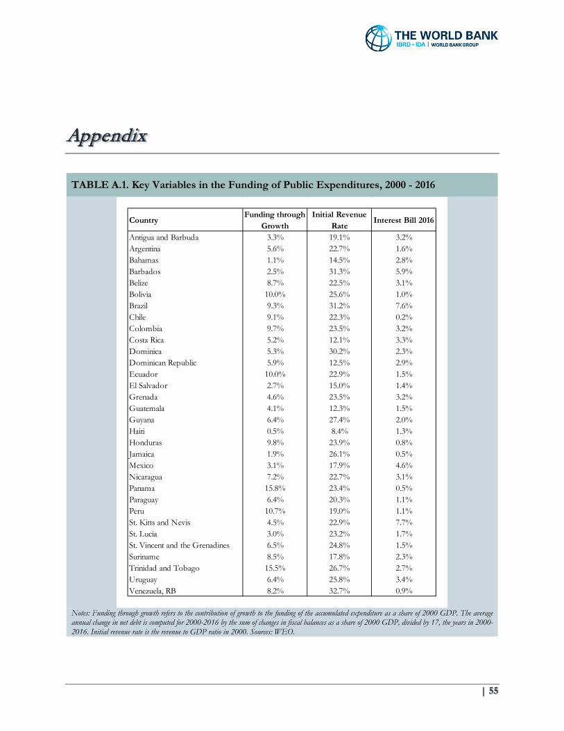
| 55
Appendix
TABLE A.1. Key Variables in the Funding of Public Expenditures, 2000 - 2016
Notes: Funding through growth refers to the contribution of growth to the funding of the accumulated expenditure as a share of 2000 GDP. The average annual change in net debt is computed for 2000-2016 by the sum of changes in fiscal balances as a share of 2000 GDP, divided by 17, the years in 2000-2016. Initial revenue rate is the revenue to GDP ratio in 2000. Sources: WEO.
CountryFunding through
GrowthInitial Revenue
RateInterest Bill 2016
Antigua and Barbuda 3.3% 19.1% 3.2%Argentina 5.6% 22.7% 1.6%Bahamas 1.1% 14.5% 2.8%Barbados 2.5% 31.3% 5.9%Belize 8.7% 22.5% 3.1%Bolivia 10.0% 25.6% 1.0%Brazil 9.3% 31.2% 7.6%Chile 9.1% 22.3% 0.2%Colombia 9.7% 23.5% 3.2%Costa Rica 5.2% 12.1% 3.3%Dominica 5.3% 30.2% 2.3%Dominican Republic 5.9% 12.5% 2.9%Ecuador 10.0% 22.9% 1.5%El Salvador 2.7% 15.0% 1.4%Grenada 4.6% 23.5% 3.2%Guatemala 4.1% 12.3% 1.5%Guyana 6.4% 27.4% 2.0%Haiti 0.5% 8.4% 1.3%Honduras 9.8% 23.9% 0.8%Jamaica 1.9% 26.1% 0.5%Mexico 3.1% 17.9% 4.6%Nicaragua 7.2% 22.7% 3.1%Panama 15.8% 23.4% 0.5%Paraguay 6.4% 20.3% 1.1%Peru 10.7% 19.0% 1.1%St. Kitts and Nevis 4.5% 22.9% 7.7%St. Lucia 3.0% 23.2% 1.7%St. Vincent and the Grenadines 6.5% 24.8% 1.5%Suriname 8.5% 17.8% 2.3%Trinidad and Tobago 15.5% 26.7% 2.7%Uruguay 6.4% 25.8% 3.4%Venezuela, RB 8.2% 32.7% 0.9%

Semiannual Report • Office of the Regional Chief Economist April 2017
The World Bank1818 H Street, NW,Washington, DC 20433, USA.www.worldbank.org/laceconomist
FISCAL POLICY IN LATIN AMERICA AND THE CARIBBEAN IN A HISTORICAL PERSPECTIVE
LEANING AGAINST THE WIND


![), pp. 209-218 - Left Business Observer review (Grand Street...Fed's mission in two oft-quoted phrases: "leaning against the wind," or, alternatively, "[taking] away the punch bowl](https://static.fdocuments.us/doc/165x107/5f0839e77e708231d420f5cf/-pp-209-218-left-business-review-grand-street-feds-mission-in-two-oft-quoted.jpg)