Leaning against the wind

Pierre-Olivier Weill∗

January 21, 2006

Abstract

During financial disruptions, marketmakers provide liquidity by absorbing external sell-

ing pressure. They buy when the pressure is large, accumulate inventories, and sell when

the pressure alleviates. This paper studies optimal dynamic liquidity provision in a the-

oretical market setting with large and temporary selling pressure, and order-execution

delays. I show that competitive marketmakers offer the socially optimal amount of

liquidity, provided they have access to sufficient capital. If raising capital is costly, this

suggests a policy role for lenient central-bank lending during financial disruptions.

Keywords: marketmaking capital, marketmaker inventory management, financial crisis.

∗Department of Finance, New York University Stern School of Business, 44 West Fourth Street, Suite9-190, New York NY 10012, e-mail: pweill@stern.nyu.edu. First version: July 2003. I am deeply indebtedto Darrell Duffie and Tom Sargent, for their supervision, their encouragements, many detailed comments andsuggestions. I also thank Narayana Kocherlakota for fruitful discussions and suggestions. I benefited fromcomments by Manuel Amador, Marco Bassetto, Bruno Biais, Vinicius Carrasco, John Y. Campbell, WilliamFuchs, Xavier Gabaix, Ed Green, Bob Hall, Ali Hortacsu, Steve Kohlhagen, Arvind Krishnamurthy, HannoLustig, Erzo Luttmer, Eva Nagypal, Lasse Heje Pedersen, Esteban Rossi-Hansberg, Tano Santos, CarmitSegal, Stijn Van Nieuwerburgh, Francois Velde, Tuomo Vuolteenaho, Ivan Werning, Randy Wright, MarkWright, Bill Zame, Ruilin Zhou, participants of Tom Sargent’s reading group at the University of Chicago,Stanford University 2003 SITE conference, and of seminar at Stanford University, NYU Economics and Stern,UCLA Anderson, Columbia GSB, Harvard University, University of Pennsylvania, University of MichiganFinance, MIT, the University of Minnesota, the University of Chicago, Northwestern University Economicsand Kellogg, the University of Texas at Austin, the Federal Reserve Bank of Chicago, the Federal ReserveBank of Cleveland, UCLA Economics, the Federal Reserve Bank of Atlanta, and THEMA. The financialsupport of the Kohlhagen Fellowship Fund at Stanford University is gratefully acknowledged. All errors aremine.

1

1 Introduction

When disruptions subject financial markets to unusually strong selling pressures, NYSE

specialists and NASDAQ marketmakers typically lean against the wind by absorbing the

market’s selling pressure and creating liquidity: they buy large quantity of assets and build

up inventories when selling pressure in the market is large, then dispose of those inventories

after that selling pressure has subsided.1 In this paper, I develop a model of optimal dynamic

liquidity provision. To explain how much and when liquidity should be provided, I solve

for socially optimal liquidity provision. I argue that some features of the socially optimal

allocation would be regarded by a policymaker as symptoms of poor liquidity provision. In

fact, these symptoms can be consistent with efficiency. I also show that when they can

maintain sufficient capital, competitive marketmakers supply the socially optimal amount

of liquidity. If capital-market imperfections prevent marketmakers from raising sufficient

capital, this suggests a policy role for lenient central-bank lending during financial disruptions.

The model studies the following scenario. In the beginning at time zero, outside investors

receive an aggregate shock which lowers their marginal utility for holding assets relative

to cash. This creates a sudden need for cash and induces a large selling pressure. Then,

randomly over time, each investor recovers from the shock, implying that the initial selling

pressure slowly alleviates. This is how I create a stylized representation of a “flight-to-

liquidity” (Longstaff (2004)) or a stock-market crash such as that of October 1987. All trades

are intermediated by marketmakers who do not derive any utility for holding assets and who

are located in a central marketplace which can be viewed, say, as the floor of the New-York

Stock Exchange. I assume the asset market can be illiquid in the sense that traders face

order-execution delays. Specifically, investors make contact with marketmakers only after

delays that are designed to represent, for example, front-end order capture, clearing, and

settlement. While one expects such delays to be short in normal times, the Brady (1988)

report suggests that they were unusually long and variable during the crash of October 1987.

Similarly, during the crash of October 1997, customers complained about “poor or untimely

execution from broker dealers” (SEC Staff Legal Bulletin No. 8 of September 9, 1998).

Lastly, McAndrews and Potter (2002) and Fleming and Garbade (2002) document payment

and transaction delays, due to disruption of the communication network after the terrorist

attacks of September 11, 2001.

1This behavior reflects one aspect of the U.S. Securities and Exchange Commission (SEC) Rule 11-b onmaintaining fair and orderly markets.

2

In this economic environment, marketmakers offer buyers and sellers quicker exchange,

what Demsetz (1968) called “immediacy”. Marketmakers anticipate that after the selling

pressure subsides, they will achieve contact with more buyers than sellers, which will allow

them then to transfer assets to buyers in two ways. They can either contact additional sellers,

which is time-consuming because of execution delays; or they can sell from their own inven-

tories, which can be done much more quickly. Therefore, by accumulating inventories early,

when the selling pressure is large, marketmakers mitigate the adverse impact on investors of

execution delays.

The socially optimal asset allocation maximizes the sum of investors’ and marketmakers’

intertemporal utility, subject to the order-execution technology. Because agents have quasi-

linear utilities, any other asset allocation could be Pareto improved by reallocating assets

and making time-zero consumption transfers. The upper panel of Figure 1 shows the socially

optimal time path of marketmakers’ inventory. (The associated parameters and modelling

assumptions are described in Section 2.) The graph shows that marketmakers accumulate

inventories only temporarily, when the selling pressure is large. Moreover, in this example, it

is not socially optimal that marketmakers start accumulating inventories at time zero when

the pressure is strongest. This suggests that a regulation forcing marketmakers to promptly

act as “buyers of last resort” could in fact result in a welfare loss. For example, if the initial

preference shock is sufficiently persistent, marketmakers acting as buyers of last resort will

end up holding assets for a very long time, which cannot be efficient given that they are not

the final holder of the asset. Lastly, when the economy is close to its steady state (interpreted

as a “normal time”) marketmakers should effectively act as “matchmakers” who never hold

assets but merely buy and re-sell instantly.

If marketmakers maintain sufficient capital, I show that the socially optimal allocation is

implemented in a competitive equilibrium, as follows. Investors can buy and sell assets only

when they contact marketmakers. Marketmakers compete for the order flow and can trade

among each other at each time. The lower panel of Figure 1 shows the equilibrium price

path. It jumps down at time zero, then increases, and eventually reaches its steady-state

level. A marketmaker finds it optimal to accumulate inventories only temporarily, when the

asset price grows at a sufficiently high rate. This growth rate compensates for the time value

of the money spent on inventory accumulation, giving a marketmaker just enough incentive

to provide liquidity. A marketmaker thus buys early at a low price and sells later at a high

price, but competition implies that the present value of her profit is zero.

Ample anecdotal evidence suggests that marketmakers do not maintain sufficient capital

3

2 4 6 8 10 12

2 4 6 8 10 12

inventory

time

price

0

0

0

Figure 1: Features of the Competitive Equilibrium.

(Brady (1988), Greenwald and Stein (1988), Mares (2001), and Greenberg (2003).) I find

that if marketmakers do not maintain sufficient capital, then they are not able to purchase as

many assets as prescribed by the socially optimal allocation. If capital-market imperfections

prevent marketmakers from raising sufficient capital before the crash, lenient central-bank

lending during the crash can improve welfare. Recall that during the crash of October 1987,

the Federal Reserve lowered the funds rate while encouraging commercial banks to lend to

security dealers (Parry (1997), Wigmore (1998).)

It is often argued that marketmakers should provide liquidity in order to maintain price

continuity and to smooth asset price movements.2 The present paper steps back from such

price-smoothing objective and instead studies liquidity provision in terms of the Pareto crite-

rion. The results indicate that Pareto-optimal liquidity provision is consistent with a discrete

price decline at the time of the crash. This suggests that requiring marketmakers to maintain

price continuity at the time of the crash might result in a welfare loss.

2For instance, the glossary of www.nyse.com states that NYSE specialists “use their capital to bridgetemporary gaps in supply and demand and help reduce price volatility.” See also the NYSE informationmemo 97-55.

4

Related Literature

Liquidity provision in normal times has been analyzed in traditional inventory-based mod-

els of marketmaking. Garman (1976), Amihud and Mendelson (1980), and Mildenstein and

Schleef (1983) study pricing and inventory management by risk-neutral monopolistic mar-

ketmakers receiving buying and selling orders at random arrival times. Stoll (1978), Ho and

Stoll (1981), and O’Hara and Oldfield (1986) study risk-averse monopolistic marketmakers

and explain the impact of return and order-flow uncertainty on bid-ask spreads. Ho and

Stoll (1983) derive some equilibrium results with competitive marketmakers. Because they

study inventory management in normal times, all of the above authors assume that supply

and demand curves are time-invariant. In contrast, I study the inventory management of

competitive marketmakers under unusual market conditions, when the market is subject to

a large and temporary selling pressure. In my model, supply and demand are time-varying.

With competitive marketmakers receiving orders at random arrival times, traditional models

would feature time variation in the cross-sectional distribution of inventories and as a result

would lose much of their tractability. The present model shortcuts this difficulty by assuming

that, at each time, marketmakers can trade among each other. Moreover, while traditional

models specify exogenous supply and demand curves, I derive them from the solutions of

investors’ intertemporal utility maximization problems. This explicit treatment of investors’

preferences facilitates welfare analysis. Lastly, the final difference with this literature is

that I address the impact of scarce marketmaking capital on marketmakers’ profit and price

dynamics.

Grossman and Miller (1988) and Greenwald and Stein (1991) analyze marketmaking dur-

ing disruptions from a risk-sharing perspective. In their model, both the sellers and the

marketmakers enter a Walrasian market in the first time period and they wait for buyers to

enter in the second. With or without marketmakers, assets are allocated to buyers in the sec-

ond period, implying that marketmakers play no role in facilitating trade between the initial

sellers and the later buyers. In the present model, by contrast, the social benefit of liquidity

provision is to facilitate trade, in that it speeds up the allocation of assets from the initial

sellers to the later buyers. Moreover Grossman and Miller study a two-period model, which

means that the timing of liquidity provision is effectively exogenous, in that marketmakers

buy in the first period and sell in the second. With its richer intertemporal structure, my

model sheds light on the optimal timing of liquidity provision. Bernardo and Welch (2004)

propose a two-period model of financial-market run, along the lines of Diamond and Dybvig

5

(1983). Their main objective is to explain the cause of a financial crisis. In the run, their

myopic marketmakers end up providing too much liquidity, prior to an uncertain aggregate

liquidity shock. The objective of the present model is not to explain the cause of a crisis but

rather to develop an intertemporal model of marketmakers optimal liquidity provision, after

an aggregate liquidity shock.

The impact of trading delays in security markets is studied by dynamic asset-pricing

models with search frictions, such as Duffie, Garleanu, and Pedersen (2004), Weill (2004),

Vayanos and Wang (2004), Spulber (1996) and Hall and Rust (2003). The present model

builds specifically on the work of Duffie, Garleanu, and Pedersen (2005). In their model,

marketmakers are matchmakers who, by assumption, cannot hold inventory. By studying

investment in marketmaking capacity, they focus on liquidity provision in the long run.

By contrast, I study liquidity provision in the short run and view marketmaking capacity

as a fixed parameter. In the short run, marketmakers provide liquidity by adjusting their

inventory positions.

Another related literature studies the equilibrium and socially optimal entry of middle-

men in search-and-matching economies (see, among others, Rubinstein and Wolinsky (1987),

Li (1998), Shevchenko (2004), and Masters (2004)). The central objective of these papers

is to characterize the size of the middlemen sector in a steady-state where the aggregate

amount of middlemen’s inventories remains constant over time. The present paper studies

intermediation during a financial crisis, when it is arguably reasonable to take the size of

the marketmaking sector as given. In the short run, the marketmaking sector can only gain

capacity by increasing its capital and aggregate inventories fluctuate over time.

The remainder of this paper is organized as follows. Section 2 describes the economic

environment, Section 3 solves for socially optimal dynamic liquidity provision, Section 4

studies the implementation of this optimum in a competitive equilibrium, and introduces

borrowing-constrained marketmakers. Section 4.2 discusses policy implications, and Section

6 concludes. The appendix contains the proofs.

2 The Economic Environment

This section describes the economy and introduces the two main assumptions of this paper.

First, there is a large and temporary selling pressure. Second, there are order-execution

delays.

6

2.1 Marketmakers and Investors

Time is treated continuously, and runs forever. A probability space (Ω,F, P ) is fixed, as well

as an information filtration Ft, t ≥ 0 satisfying the usual conditions (Protter (1990)). The

economy is populated by a non-atomic continuum of infinitely lived and risk-neutral agents

who discount the future at the constant rate r > 0. An agent enjoys the consumption of a

non-storable numeraire good called “cash,” with a marginal utility normalized to 1.3

There is one asset in positive supply. An agent holding q units of the asset receives a

stochastic utility flow θ(t)q per unit of time. Stochastic variations in the marginal utility θ(t)

capture a broad range of trading motives such as changes in hedging needs, binding borrowing

constraints, changes in beliefs, or risk-management rules such as risk limits. There are two

types of agents, marketmakers and investors, with a measure one (without loss of generality)

of each. Marketmakers and investors differ in their marginal-utility processes θ(t), t ≥ 0, as

follows. A marketmaker has a constant marginal utility θ(t) = 0 while an investor’s marginal

utility is a two-state Markov chain: the high-marginal-utility state is normalized to θ(t) = 1,

and the low-marginal-utility state is θ(t) = 1 − δ, for some δ ∈ (0, 1). Investors transit

randomly, and pair-wise independently, from low to high marginal utility with intensity4 γu,

and from high to low marginal utility with intensity γd.

These independent variations over time in investors’ marginal utilities create gains from

trade. A low-marginal-utility investor is willing to sell his asset to a high-marginal-utility

investor in exchange for cash. A marketmaker’s zero marginal utility could capture a large

exposure to the risk of the market she intermediates. In addition, it implies that in the equi-

librium to be described, a marketmaker will not be the final holder of the asset. In particular,

a marketmaker would choose to hold assets only because she expects to make some profit by

buying and reselling.5

Asset Holdings

The asset has s ∈ (0, 1) shares outstanding per investor’s capita. Marketmakers can hold any

positive quantity of the asset. The time t asset inventory I(t) of a representative marketmaker

3Equivalently, one could assume that agents can borrow and save cash in some “bank account,” at theinterest rate r = r. Section 4 adopts this alternative formulation.

4For instance, if θ(t) = 1 − δ, the time infu ≥ 0 : θ(t+ u) 6= θ(t) until the next switch is exponentiallydistributed with parameter γu. The successive switching times are independent.

5The results of this paper hold under the weaker assumption that marketmakers’ marginal utility isθ(t) = 1 − δM , for some holding cost δM > δ. Proofs are available from the author upon request.

7

satisfies the short-selling constraint6

I(t) ≥ 0. (1)

An investor also cannot short-sell and, moreover, he cannot hold more than one unit of the

asset. This paper restricts attention to allocations in which an investor holds either zero or

one unit of the asset. In equilibrium, because an investor has linear utility, he will find it

optimal to hold either the maximum quantity of one or the minimum quantity of zero.

An investor’s type is made up of his marginal utility (high “h,” or low “ℓ”) and his

ownership status (owner of one unit, “o,” or non-owner, “n”). The set of investors’ types

is T ≡ ℓo, hn, ho, ℓn. In anticipation of their equilibrium behavior, low-marginal-utility

owners (ℓo) are named “sellers,” and high-marginal-utility non-owners (hn) are “buyers.”

For each σ ∈ T, µσ(t) denotes the fraction of type-σ investors in the total population of

investors. These fractions must satisfy two accounting identities. First, of course,

µℓo(t) + µhn(t) + µℓn(t) + µho(t) = 1. (2)

Second, the assets are held either by investors or marketmakers, so

µho(t) + µℓo(t) + I(t) = s. (3)

2.2 Crash and Recovery

I select initial conditions representing the strong selling pressure of a financial disruption.

Namely, it is assumed that, at time zero, all investors are in the low-marginal-utility state

(see Table 1). Then, as earlier specified, investors transit to the high-marginal-utility state.

Under suitable measurability requirements (see Sun (2000), Theorem C), the Law of Large

Numbers applies, and the fraction µh(t) ≡ µho(t) + µhn(t) of high-marginal-utility investors

solves the ordinary differential equation (ODE)

µh(t) = γu(

µℓo(t) + µℓn(t))

− γd(

µho(t) + µhn(t))

(4)

= γu(

1 − µh(t))

− γdµh(t)

= γu − γµh(t),

where µh(t) = dµh(t)/dt and γ ≡ γu + γd. The first term in (4) is the rate of flow of low-

marginal-utility investors transiting to the high-marginal-utility state, while the second term

6One can show that, in the present setup, choosing I(t) ≥ 0 is optimal as long as marketmakers incur aflow cost c > 1 − δγd/(r + ρ+ γu + γd) per unit of negative inventory. This cost could capture, for example,the fact that short positions typically involve larger transaction costs and are more risky than long positions.

8

0 2 4 8 10 12 140

0.05

0.1

0.15

0.2

0.25

0.3

0.35

0.4

µhs

ts time (hours)

Figure 2: Dynamic of µh(t).

is the rate of flow of high-marginal-utility investors transiting to the low-marginal-utility

state. With the initial condition µh(0) = 0, the solution of (4) is

µh(t) = y(

1 − e−γt)

, (5)

where y ≡ γu/γ is the steady-state fraction of high-marginal-utility investors. Importantly

for the remainder of the paper, it is assumed that

s < y. (6)

In other words, in steady state, the fraction y of high-marginal-utility investors exceeds the

asset supply s. This will ensure that, asymptotically in equilibrium, the selling pressure has

fully alleviated. Figure 2 plots the time dynamic of µh(t), for some parameter values that

satisfy (6). On the Figure, the unit of time is one hour. Years are converted into hours

assuming 250 trading days per year, and 10 hours of trading per days. The parameter values

used for all of the illustrative computations of this paper, are in Table 2.

Table 1: Initial conditions.

µℓo(0) µhn(0) µℓn(0) µho(0) I(0)

s 0 1 − s 0 0

9

Table 2: Parameter Values.

Parameters Value

Measure of Shares s 0.2Discount Rate r 5%Contact Intensity ρ 1000Intensity of Switch to High γu 90Intensity of Switch to Low γd 10Low marginal utility 1 − δ 0.01

Time is measured in years. Assuming that the stock market opens250 days a year, ρ = 1000 means that it takes 2.5 hours to executean order, on average. The parameter γ = γu + γd measures thespeed of the recovery. Specifically, with γ = 100, µh(t) reacheshalf of its steady-state level in about 1.73 days.

2.3 Order-execution delays

This paper departs from the traditional Walrasian model by assuming that the asset market is

illiquid, in that there are order-execution delays. Marketmakers intermediate all trades from

a central marketplace which can be viewed, say, as the floor of the New York Stock exchange.

The asset market is illiquid in the sense that investors cannot contact that marketplace

instantly. Instead, an investor establishes contact with marketmakers at Poisson arrival

times with intensity ρ > 0. Contact times are pairwise independent across investors and

independent of marginal utility processes. Therefore, an application of the Law of Large

Numbers (under the technical conditions mentioned earlier) implies that contacts between

type-σ investors and marketmakers occur at a total (almost sure) rate of ρµσ(t). Hence, in a

market equilibrium, ρµσ(t) represents the order-flow rate originating from type-σ investors.7

The random contact times represent a broad range of execution delays, including the

time to contact a marketmaker, to negotiate and process an order, to deliver an asset, or

to transfer a payment. The parameter ρ is viewed as a measure of marketmaking capac-

ity, encompassing for instance the communication network and the infrastructures needed

to execute transactions. One might argue that execution delays are usually quite short and

perhaps therefore of little consequence to the quality of an allocation. The Brady (1988)

7An alternative specification would let the instantaneous rate of contact with type-σ investors be someincreasing and strictly concave function of µσ(t). This would capture congestions, as the average contacttimes would be decreasing in µσ(t). This alternative non-linear specification is however much less tractableand requires a numerical solution method. Moreover, one might expect that the basic intuitions for thewelfare improving role of marketmakers’ liquidity provision would be the same as with the present linearspecification.

10

report shows, however, that during the October 1987 crash, delays were much longer and

much more variable than in normal times. In particular, the report documents that many

delays were caused by failures of overloaded execution systems, by congestions in the com-

munication network, and by automated protection features. The report suggests that such

delays might have amplified liquidity problems in a far-from-negligible manner.8

Delays also occurred during the crash of October 1997. The SEC reported that “broker-

dealers web servers had reached their maximum capacity to handle simultaneous users”

and “telephone lines were overwhelmed with callers who were frustrated by the inability to

access information online.” As a result of these capacity problems, customers could not be

“routed to their designated market center for execution on a timely basis” and “a number

of broker dealers were forced to manually execute some customers orders.”9 This suggests

that technological improvements which followed the 1987 crash did not prevent substantial

order-execution delays from arising during the crash of 1997.

3 Optimal Dynamic Liquidity Provision

The first objective of this section is to explain the benefit of liquidity provision, addressing

how much and when liquidity should be provided. Its second objective is to establish a

benchmark against which to judge the market equilibria studied in Sections 4 and 4.2. To

these ends, I temporarily abstract from marketmakers’ incentives to provide liquidity and

solve for socially optimal allocations, maximizing the sum of investors and marketmakers’

intertemporal utility, subject to order-execution delays. The optimal allocation is found to

resemble “leaning against the wind.” Namely, it is socially optimal that a marketmaker

accumulates inventories when the selling pressure is strong.

3.1 Asset Allocations

At each time, a representative marketmaker can transfer assets only to her own account

or among those of investors who are currently contacting her. For instance, the flow rate

uℓ(t) of assets that a marketmaker takes from low-marginal-utility investors is subject to the

8After describing the selling pressure originating from portfolio insurers, the report notes:“Transactionsystems, such as DOT, or market stabilizing mechanisms, such as NYSE specialists, are bound to be crushedby the pressure, however they are designed or capitalized.” See also Wigmore (1998).

9SEC Staff Legal Bulletin No. 8, http://www.sec.gov/interps/legal/slbmr8.htm

11

order-flow constraint

−ρµℓn(t) ≤ uℓ(t) ≤ ρµℓo(t). (7)

The upper (lower) bound shown in (7) is the flow of ℓo (ℓn) investors who establish contact

with marketmakers at time t. Similarly, the flow uh(t) of assets that a marketmaker transfers

to high-marginal-utility investors is subject to the order-flow constraint

−ρµho(t) ≤ uh(t) ≤ ρµhn(t). (8)

When the two flows uℓ(t) and uh(t) are equal, a marketmaker is a matchmaker, in the sense

that she takes assets from some ℓo investors (sellers) and transfers them instantly to some hn

investors (buyers). If the two flows are not equal, a marketmaker is not only matching buyers

and sellers, but she is also changing her inventory position. For example, if both uℓ(t) and

uh(t) are positive, a marketmaker is matching sellers and buyers at the rate minuℓ(t), uh(t).The net flow uℓ(t)−uh(t) represents the rate of change of a marketmaker’s inventory, in that

I(t) = uℓ(t) − uh(t). (9)

Similarly, the rate of change of the fraction µℓo(t) of low-marginal-utility owners is

µℓo(t) = −uℓ(t) − γuµℓo(t) + γdµho(t), (10)

where the terms γuµℓo(t) and γdµho(t) reflect transitions of investors from low to high marginal

utility, and from high to low marginal utility, respectively. Likewise, the rate of change of

the fractions of hn, ℓn, and ho investors are, respectively,

µhn(t) = −uh(t) − γdµhn(t) + γuµℓn(t) (11)

µℓn(t) = uℓ(t) − γuµℓn(t) + γdµhn(t) (12)

µho(t) = uh(t) − γdµho(t) + γuµℓo(t). (13)

Definition 1 (Feasible Allocation). A feasible allocation is some distribution µ(t) ≡(

µσ(t))

σ∈Tof types, some inventory holding I(t), and some piecewise continuous asset flows

u(t) ≡(

uh(t), uℓ(t))

such that

(i) At each time, the short-selling constraint (1) and the order-flow constraints (7)-(8) are

satisfied.

12

(ii) The ODEs (9)-(13) hold.

(iii) The initial conditions of Table 1 hold.

Since u(t) is piecewise continuous, µ(t) and I(t) are piecewise continuously differentiable.

A feasible allocation is said to be constrained Pareto optimal if it cannot be Pareto

improved by choosing another feasible allocation and making time-zero cash transfers. As it

is standard with quasi-linear preferences, it can be shown that a constrained Pareto optimal

allocation must maximize∫ +∞

0

e−rt(

µho(t) + (1 − δ)µℓo(t)

)

dt, (14)

the equally weighted sum of investors’ intertemporal utilities for holding assets.10 This cri-

terion is deterministic, reflecting pairwise independence of investors’ marginal-utility and

contact-time processes. Conversely, an asset allocation maximizing (14) is constrained Pareto

optimal. This discussion motivates the following definition of an optimal allocation.

Definition 2 (Socially Optimal Allocation). A socially optimal allocation is some feasible

allocation maximizing (14).

3.2 The Cost and Benefit of Liquidity Provision

This subsection illustrates the social benefits of accumulating inventories. Namely, it consid-

ers the no-inventory allocation (I(t) = 0, at each time), and shows that it can be improved if

marketmakers accumulate a small amount of inventory, when the selling pressure is strong.

I start by describing some features of the no-inventory allocation. Substituting I(t) = 0 into

equation (3) gives

µℓo(t) = s− µh(t) + µhn(t). (15)

The “crossing time” is the time ts at which µh(ts) = s. This is, as Figure 2 illustrates, the

time at which the fraction µh(t) of high-marginal-utility investors crosses the supply s of

assets. Because µh(t) is increasing, equation (15) implies that

ρµhn(t) < ρµℓo(t) (16)

10Marketmakers intertemporal utility for holding assets is equal to zero and hence does not appear in(14). If a marketmaker marginal utility for holding asset is (1 − δM ) > 0, then one has to add a term∫

∞

0e−rt(1 − δM )I(t) dt to the above criterion.

13

if and only if t < ts. Therefore, in the no-inventory allocation, before the crossing time, the

selling pressure is “positive,” meaning that marketmakers are in contact with more sellers

(ℓo) than buyers (hn). After the crossing time, they are in contact with more buyers than

sellers.

Intuitively, the no-inventory allocation can be improved as follows. A marketmaker can

take an additional asset from a seller before the crossing time, say at t1 = ts−ε, and transfer

it to some buyer after the crossing time, at t2 = ts + ε. Because the transfer occurs around

the crossing time, the transfer time 2ε can be made arbitrarily small.

The benefit is that, for a sufficiently small ε, this asset is allocated almost instantly

to some high-marginal-utility investor. Without the transfer, by contrast, this asset would

continue to be held by a low-marginal-utility investor until either i) the seller transits to

a high marginal utility with intensity γu, or ii) the seller establishes another contact with

a marketmaker with intensity ρ. This means that, without the transfer, this asset would

continue to be held by a seller and not by a buyer, with an instantaneous utility cost of δ,

incurred for a non-negligible average time of 1/(γu + ρ).

The cost of the transfer is that the asset is temporarily held by a marketmaker and not

by a seller, implying an instantaneous utility cost of 1− δ. If ε is sufficiently small, this cost

is incurred for a negligible time and is smaller than the benefit. This intuitive argument can

be formalized by studying the following family of feasible allocations.

Definition 3 (Buffer Allocation). A buffer allocation is a feasible allocation defined by

two times (t1, t2) ∈ [0, ts] × [ts,+∞), called “breaking times,” such that11

uℓ(t) = ρµhn(t)I[0,t1)(t) + ρµℓo(t)I[t1,+∞)(t) (17)

uh(t) = ρµhn(t)I[0,t2)(t) + ρµℓo(t)I[t2,+∞)(t) (18)

I(t2) = 0. (19)

The no-inventory allocation is the buffer allocation for which t1 = t2 = ts. A buffer allocation

has the “bang-bang” property: at each time, either uℓ(t) = ρµℓo(t) or uh(t) = ρµhn(t).

Because of the linear objective (14), it is natural to guess that a socially optimal allocation

will also have this bang-bang property. In the next subsection, Theorem 1 will confirm

this conjecture, showing that the socially optimal allocation belongs to the family of buffer

allocations.

11In what follows, IA( · ) denotes the indicator function of some set A ⊆ R.

14

0 2 6 10 12 14

0

10

30

40

time (hours)

I(t)/s (%)

t1 t2

m/s

Figure 3: Illustrative Buffer Allocations.

In a buffer allocation, a marketmaker acts as a “buffer,” in that she accumulates assets

when the selling pressure is strong and unwinds these trades when the pressure alleviates.

Specifically, as illustrated in Figure 3, a buffer allocation (t1, t2) has three phases. In the

first phase, when t ∈ [0, t1], a marketmaker does not accumulate inventory (uℓ(t) = uh(t) and

I(t) = 0). In the second phase, when t ∈ (t1, t2), a marketmaker first builds up (uℓ(t) > uh(t)

and I(t) > 0) and then unwinds (uℓ(t) < uh(t) and I(t) > 0) her inventory position. At

time t2, her inventory position reaches zero. In the third phase t ∈ [t2,+∞), a marketmaker

does not accumulate inventory (uℓ(t) = uh(t) and I(t) = 0). The following proposition

characterizes buffer allocations by the maximum inventory position held by marketmakers.

Proposition 1. There exist some m ∈ R+, some strictly decreasing continuous function ψ :

[0, m] → R+, and some strictly increasing continuous functions φi : [0, m] → R+, i ∈ 1, 2,such that, for all m ∈ [0, m] and all buffer allocations (t1, t2),

m = maxt∈R+

I(t) (20)

ψ(m) = arg maxt∈R+

I(t) (21)

t1 = ψ(m) − φ1(m) (22)

t2 = ψ(m) + φ2(m), (23)

where m is the unique solution of ψ(z) − φ1(z) = 0. Furthermore, ψ(0) = ts and φ1(0) =

φ2(0) = 0.

In words, the breaking times (t1, t2) of a buffer allocation can be written as functions of the

maximum inventory position m. The maximum inventory position is achieved at time ψ(m).

15

0 5 10 15 30 35 40 45

m/s (%)

C(m)

m/s

0

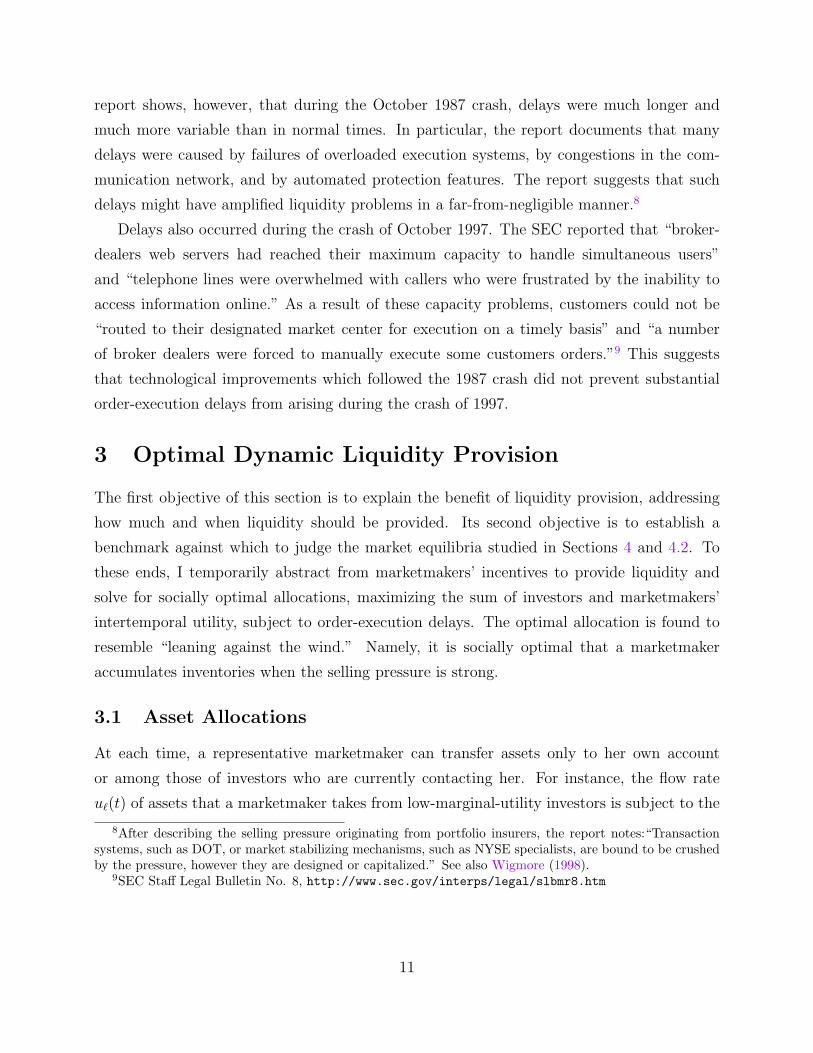
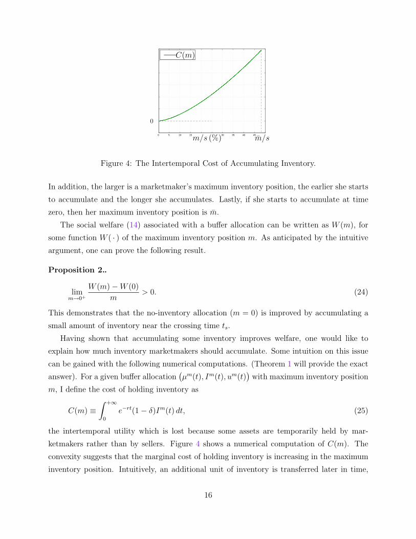
Figure 4: The Intertemporal Cost of Accumulating Inventory.

In addition, the larger is a marketmaker’s maximum inventory position, the earlier she starts

to accumulate and the longer she accumulates. Lastly, if she starts to accumulate at time

zero, then her maximum inventory position is m.

The social welfare (14) associated with a buffer allocation can be written as W (m), for

some function W ( · ) of the maximum inventory position m. As anticipated by the intuitive

argument, one can prove the following result.

Proposition 2..

limm→0+

W (m) −W (0)

m> 0. (24)

This demonstrates that the no-inventory allocation (m = 0) is improved by accumulating a

small amount of inventory near the crossing time ts.

Having shown that accumulating some inventory improves welfare, one would like to

explain how much inventory marketmakers should accumulate. Some intuition on this issue

can be gained with the following numerical computations. (Theorem 1 will provide the exact

answer). For a given buffer allocation(

µm(t), Im(t), um(t))

with maximum inventory position

m, I define the cost of holding inventory as

C(m) ≡∫ +∞

0

e−rt(1 − δ)Im(t) dt, (25)

the intertemporal utility which is lost because some assets are temporarily held by mar-

ketmakers rather than by sellers. Figure 4 shows a numerical computation of C(m). The

convexity suggests that the marginal cost of holding inventory is increasing in the maximum

inventory position. Intuitively, an additional unit of inventory is transferred later in time,

16

0 5 10 15 30 35 40 45

m/s (%)

B(m)

m/s

Figure 5: The Intertemporal Benefit of Accumulating inventory.

implying that the holding cost 1−δ is incurred for a longer time period. Similarly, the benefit

of holding inventory is implicitly defined by

W (m) ≡ B(m) − C(m). (26)

That is, B(m) = W (m) +C(m) is a measures of social welfare which is compensated for the

holding cost 1− δ of a marketmaker. Figure 5 shows a numerical computation of B(m). The

concavity suggests that the marginal benefit of accumulating inventory is decreasing in the

maximum inventory position: an additional unit of inventory is transferred to a buyer later

in time, which represents a smaller benefit because agents are impatient. Interestingly, B( · )decreases above some inventory level. In this decreasing branch, marketmakers take too long

to transfer a marginal unit. It would be faster, on average, to simply wait for the ℓo investors

to transit to the high-marginal-utility state.

Overall, these computations suggest that providing liquidity is cheap and valuable near

the crossing time (m close to zero). By contrast, providing liquidity near time zero, when the

selling pressure is strongest (m close to m), is both more expensive and less valuable. The

marginal social value of providing liquidity near time zero can even be negative, as illustrated

by Figures 4 and 5.

3.3 The Socially Optimal Allocation

This subsection provides first-order sufficient conditions for, and solves for, a socially optimal

allocation. The reader may wish to skip the following paragraph on first-order conditions,

and go directly to Theorem 1, which describes the socially optimal allocation.

17

First-Order Sufficient Conditions

The first-order sufficient conditions are based on Seierstad and Sydsæter (1977). The ac-

counting identities µho(t) = µh(t) − µhn(t) and µℓn(t) = 1 − µh(t) − µℓn(t) are substituted

into the objective and the constraints, reducing the state variables to(

µℓo(t), µhn(t), I(t))

.

The “current-value” Lagrangian (see Kamien and Schwartz (1991), Part II, Section 8) is

L(t) = µh(t) − µhn(t) + (1 − δ)µℓo(t) (27)

+λℓ(t)(

−uℓ(t) − γuµℓo(t) − γdµhn(t) + γdµh(t))

−λh(t)(

−uh(t) − γuµℓo(t) − γdµhn(t) + γu(1 − µh(t)))

+λI(t)(

uℓ(t) − uh(t))

+wℓ(t)(

ρµℓo(t) − uℓ(t))

+ wh(t)(

ρµhn(t) − uh(t))

+ ηI(t) I(t).

The multiplier λℓ(t) of the ODE (10) represents the social value of increasing the flow of

investors from the ℓn type to the ℓo type or, equivalently, the value of transferring an asset

to an ℓn investor. One gives a similar interpretation to the multipliers λh(t) and λI(t) of the

ODEs (11) and (9), respectively.12 The multipliers wℓ(t) and wh(t) of the flow constraints (7)

and (8) represent the social value of increasing the rate of contact with ℓo and hn investors,

respectively.13 The multiplier on the short-selling constraint (1) is ηI(t). The first-order

condition with respect to the controls uℓ(t) and uh(t) are

wℓ(t) = λI(t) − λℓ(t) (28)

wh(t) = λh(t) − λI(t), (29)

respectively. For instance, (28) decomposes wℓ(t) into the opportunity cost −λℓ(t) of taking

assets from ℓo investors, and the benefit λI(t) of increasing a marketmaker’s inventory. The

positivity and complementary-slackness conditions for wℓ(t) and wh(t), respectively, are

wℓ(t) ≥ 0 and wℓ(t)(

ρµℓo(t) − uℓ(t))

= 0, (30)

wh(t) ≥ 0 and wh(t)(

ρµhn(t) − uh(t))

= 0. (31)

The multipliers wℓ(t) and wh(t) are non-negative because a marketmaker can ignore addi-

tional contacts. The complementary-slackness condition (30) means that, when the marginal

12In equation (27), the minus sign in front of λh(t) is contrary to conventional notations but turns out tosimplify the exposition.

13It is anticipated that the left-hand constraints in (7) and (8) never bind. In other words, a marketmakernever transfers asset from a high-marginal-utility to a low-marginal-utility investor.

18

value wℓ(t) of additional contact is strictly positive, a marketmaker should take the assets

of all ℓo investors with whom she is currently in contact. One also has the positivity and

complementary-slackness conditions

ηI(t) ≥ 0 and ηI(t)I(t) = 0. (32)

The ODE for the the multipliers λℓ(t), λh(t), and λI(t) are

rλℓ(t) = 1 − δ + γu(λh(t) − λℓ(t)) + ρwℓ(t) + λℓ(t) (33)

rλh(t) = 1 + γd(λℓ(t) − λh(t)) − ρwh(t) + λh(t) (34)

rλI(t) = ηI(t) + λI(t), (35)

respectively. For instance, (33) decomposes the flow value rλℓ(t) of transferring an asset to

a low-marginal-utility investor. The first term, 1 − δ, is the flow marginal utility of a low-

marginal-utility investor holding one unit of the asset. The second term, γu(

λh(t)−λℓ(t))

, is

the expected rate of net utility associated with a transition to high marginal utility. That is,

with intensity γu, λℓ(t) becomes the value λh(t) of transferring an asset to a high-marginal-

utility investor. The third term, ρwℓ(t), is the expected rate of net utility of a contact

between an ℓo investor and a marketmaker. The multipliers(

λℓ(t), λh(t), λI(t))

must satisfy

the following additional restrictions. First, they must satisfy the transversality conditions14

limt→+∞

λj(t)e−rt = 0, (36)

for j ∈ ℓ, h, I. Second, the multipliers λh(t) and λℓ(t) are continuous. Because the control

variable u(t) does not appear in the short-selling constraint I(t) ≥ 0, however, the multiplier

λI(t) might jump, with the restriction that

λI(t+) − λI(t

−) ≤ 0 if I(t) = 0. (37)

In other words, the multiplier λI(t) can jump down, but only when the short-selling con-

straint is binding. Intuitively, if λI(t) were to jump up at t, a marketmaker could accu-

mulate additional inventory shortly before t, say a quantity ε, improving the objective by

ε(

λI(t+) − λI(t

−))

e−rt.15

14This condition allows to complete the standard optimality verification argument when the time horizonis infinite.

15Because the ODEs for the state variables are linear, the first-order sufficient conditions impose no signrestriction on the multipliers λh(t), λℓ(t), and λI(t) (see Section 3 in Part II of Kamien and Schwartz (1991)).

19

The Socially Optimal Allocation

Appendix B guesses and verifies that the (essentially unique) socially optimal allocation is

a buffer allocation. Namely, for a given buffer allocation, one constructs multipliers solving

the first-order conditions (28) through (37). The restriction wℓ(t1) = 0 is used to find the

breaking-times t1 and t2.

Theorem 1 (Socially optimal Allocation). There exists a socially optimal allocation(

µ∗(t), I∗(t), u∗(t), t ≥ 0)

. This allocation is a buffer allocation with breaking times (t∗1, t∗2)

determined by

e−γt∗

1 =

(

1 − s

y

)

1 − e−ρ∆∗

ρ

ρ− γ

e−γ∆∗ − e−ρ∆∗(38)

t∗2 = t∗1 + ∆∗ (39)

∆∗ = min

1

r + ρlog

(

1 +δ(r + ρ)

γu + (1 − δ)(r + ρ+ γd)

)

, ∆

,

where ∆ ≡ φ1(m) + φ2(m) and, if γ = ρ, one lets (e−γx − e−ρx)/(ρ− γ) ≡ x for all x ∈ R.

If ∆∗ = ∆, the first breaking time is t∗1 = 0, meaning that a marketmaker starts accumulating

inventory at the time of the “crash.”

The socially optimal allocation has three main features. First, it is optimal that a market-

maker provides some liquidity: From time t∗1 to time t∗2, she builds up and unwinds a positive

inventory position. Second, it is not necessarily optimal that a marketmaker provides liq-

uidity at time zero, when the selling pressure is strongest. This suggests that, although a

marketmaker should provide liquidity, she should not act as a “buyer of last resort.” Third,

when the economy is close to its steady state, interpreted as a normal time, a marketmaker

should act as a mere matchmaker, meaning that she should buy and sell instantly. Thus, the

socially optimal allocation draws a sharp distinction between socially optimal marketmaking

in a normal time of low selling pressure, versus a bad time of strong selling pressure.

Proposition 3 (Uniqueness). If(

µ(t), I(t), u(t))

is a socially optimal allocation, then

µ(t) = µ∗(t) and I(t) = I∗(t), for all t ∈ R+.

3.4 Comparative Statics

A natural measure of the amount of liquidity provided by marketmakers is the length ∆∗

of the inventory-accumulation period. Another measure would be the maximum inventory

20

position m∗, which is strictly monotonic with ∆∗, provided that ρ and γ are held constant.16

With Theorem 1, ∆∗ can be written as F (ρ, r, δ, γu, γd), for some continuous function F ( · ).The following proposition provides some natural comparative statics.

Proposition 4 (A Comparative Static). Let x = (ρ, r, δ, γu, γd) be a vector of exogenous

parameters. If F (x) < ∆, then F ( · ) is differentiable at x, with partial derivatives

∂F

∂ρ< 0,

∂F

∂r< 0,

∂F

∂δ> 0,

∂F

∂γd< 0, and

∂F

∂γu< 0. (40)

If, on the other hand, F (x) = ∆, then marketmakers provide the maximum amount of liq-

uidity, in that they start accumulating inventory at time zero, when the selling pressure is

strongest. In that case, locally, F ( · ) does not depend on (r, δ). Proposition 4 shows that

the inventory-accumulation period is longer when an investor’s holding cost δ is larger. It

is shorter whenever the order-execution technology is faster, the agents are more impatient,

or investors’ switching intensities γd and γu are larger. This last comparative static reflects

the fact that larger γd and γu reduce the net utility of transferring the asset. Namely, with a

larger γd, an investor keeps a high marginal utility for a shorter time, on average. As a result,

the net utility of transferring the asset to an hn investor is smaller. With a larger γu, an

ℓo investor transits faster to a high marginal utility. This increases the value of leaving the

asset to this ℓo investor, and waiting for him to transit to the ho type. Hence, this decreases

the net utility of transferring the asset.

Walrasian Limit

This paragraph studies the socially optimal allocation as ρ goes to infinity, interpreted as

the Walrasian limit with no execution delay. This comparative static exercise illustrates the

crucial role of order-execution delays in making it optimal for a marketmaker to provide

some amount of liquidity to investors. Specifically, it is shown that, in the limit ρ→ +∞, a

marketmaker should not provide any liquidity.

Theorem 1 implies that the length ∆∗ of the inventory-accumulation period goes to

zero. This does not immediately imply that the maximum inventory position, m∗ = (φ1 +

φ2)−1(∆∗), goes to zero. Although marketmakers accumulate inventories during increasingly

16Specifically, m∗ = (φ1 + φ2)−1(∆∗), where φ1(m) and φ2(m) are increasing in m. These two functions,

however, implicitly depend on ρ and γ.

21

small time periods as ρ → +∞, they also accumulate inventories increasingly quickly. The

following proposition settles this issue.

Proposition 5 (Walrasian Limit). Given some (r, δ, γu, γd), as ρ→ +∞,

F (ρ, r, δ, γu, γd) → 0 (41)

(φ1 + φ2)−1 F (ρ, r, δ, γu, γd) → 0. (42)

As the average execution delay 1/ρ approaches zero, an asset can be transferred almost

instantly to some high-marginal-utility investor. Then, the inventory holding cost is large

relative to the benefit of providing liquidity. In such circumstances, a marketmaker should

hold a smaller quantity of the asset, for a shorter time.

4 Market Equilibrium

This section studies marketmakers’ incentives to provide liquidity. I show that the socially

optimal allocation can be implemented in a competitive equilibrium as long as they have

access to sufficient capital.

4.1 Competitive Marketmakers

This subsection describes a competitive market structure that implements the socially opti-

mal allocation.

It is assumed that a marketmaker has access to some bank account earning the constant

interest rate r = r. At each time t, she buys a flow uℓ(t) ∈ R+ of assets, sells a flow

uh(t) ∈ R+, and consumes cash at the positive rate c(t) ∈ R+. She takes as given the asset

price path

p(t), t ≥ 0

. Hence, her bank account position a(t) and her inventory position

I(t) evolve according to

a(t) = ra(t) + p(t)(

uh(t) − uℓ(t))

− c(t) (43)

I(t) = uℓ(t) − uh(t). (44)

In addition, she faces the borrowing and short-selling constraints

a(t) ≥ 0 (45)

I(t) ≥ 0. (46)

22

Lastly, at time zero, a marketmaker holds no inventory (I(0) = 0) and maintains a strictly

positive amount of capital a(0). This subsection restricts attention to some large a(0), in the

sense that the borrowing constraint (45) does not bind in equilibrium. (This statement is

made precise by Theorem 2 and Proposition 6.) The marketmaker’s objective is to maximize

the present value

∫ +∞

0

e−rtc(t) dt (47)

of her consumption stream with respect to

a(t), I(t), uℓ(t), uh(t), c(t), t ≥ 0

, subject to the

constraints (43)-(46), and the constraint that uℓ(t) and uh(t) are piecewise continuous.17

Let’s turn to the investor’s problem. An investor establishes contact with some market-

maker at Poisson arrival times with intensity ρ > 0. Conditional on establishing contact at

time t, he can buy or sell the asset at price p(t). I solve the investor’s problem using a “guess

and verify” method. Specifically, I guess that, in equilibrium, an ℓo (hn) investor always

finds it weakly optimal to sell (buy). If an ℓo (hn) investor is indifferent between selling and

not selling, he might choose not to sell (buy). Lastly, I guess that investors of types ℓn and

ho never trade. The time-t continuation utility of an investor of type σ ∈ T who follows this

policy is denoted Vσ(t). Hence, a seller’s reservation value is ∆Vℓ(t) ≡ Vℓo(t) − Vℓn(t), and a

buyer’s reservation value is ∆Vh(t) ≡ Vho(t)−Vhn(t). Appendix C.1 provides ODEs for these

continuation utilities and reservation values, as well as a precise definition of a competitive

equilibrium. The main result of this subsection states that the optimal allocation can be

implemented in some equilibrium:

Theorem 2 (Implementation). There exists some a∗0 ∈ R+ such that, for all a(0) ≥ a∗0,

there exists a competitive equilibrium whose allocation is the optimal allocation.

The proof identifies the price and the reservation values with the Lagrange multipliers of the

socially optimal allocation (see Table 3). For instance, the asset price p(t) is equal to the

multiplier λI(t) for the ODE I(t) = uℓ(t)−uh(t), interpreted as the social value of increasing

the inventory position of a marketmaker. Also, Table 3 and the complementary slackness

condition (30) imply that, before the first breaking time t∗1, wℓ(t) = p(t) − ∆Vℓ(t) = 0. In

other words, because the socially optimal allocation prescribes that marketmakers do not ac-

commodate the selling pressure, the social value wℓ(t) of increasing the rate of contact with

17The above formulation implies that, in equilibrium, if the borrowing constraint (45) never binds, amarketmaker’s intertemporal utility is equal to a(0), meaning that equilibrium net profit must be equal tozero.

23

Table 3: Identifying Prices with Multipliers.

Equilibrium Objects Multipliers Constraints

p(t) λI(t) I(t) = uℓ(t) − uh(t)

∆Vℓ(t) λℓ(t) µℓo(t) = −uℓ(t) . . .

p(t) − ∆Vℓ(t) wℓ(t) uℓ(t) ≤ ρµℓo(t)

∆Vh(t) λh(t) µhn(t) = −uh(t) . . .

∆Vh(t) − p(t) wh(t) uh(t) ≤ ρµhn(t)

In a given row, the equilibrium object in the first column isequal to the Lagrange multiplier in the second column. Thethird column describes the constraints associated with these mul-tipliers. For instance, in the first row, the price p(t) (first col-umn) is equal to the multiplier λI(t) (second column) of the ODEI(t) = uℓ(t) − uh(t) (third column).

sellers is zero. In equilibrium, this means that the price adjusts so that sellers are indifferent

between selling and not selling.

Equilibrium Price Path and Marketmakers’ Incentive

Appendix B.2 derives closed-form solutions for the equilibrium price path p(t) and the reser-

vation values ∆Vℓ(t) and ∆Vh(t). The price path, shown in the lower panel of Figure

6, jumps down at time zero, then increases, and eventually stabilizes at its steady-state

level.18 The price path reflects the three phases of the socially optimal allocation: before

the first breaking time t∗1, sellers are indifferent between selling or not selling, meaning that

p(t) = ∆Vℓ(t) = λℓ(t). Moreover, equation (33) shows that the growth rate p(t)/p(t) of the

price is strictly less than r− (1− δ)/p(t). This is because a seller with marginal utility 1− δ

does not need a large capital gain to be willing to hold the asset. By contrast, in between

the two breaking times t∗1 and t∗2, marketmakers accommodate all of the selling pressure. As

a result, the “marginal investor” is a marketmaker and p(t) > ∆Vℓ(t), meaning that the

liquidity provision of marketmakers raises the asset price above a seller’s reservation value.

Moreover, equation (35) shows that the price grows at the higher rate p(t)/p(t) = r, implying

18A simple way to construct the initial price jump is to start the economy in steady state at t = 0 andassume that agents anticipate a crash at some Poisson arrival time with intensity κ. One can show thatthe results of this paper would apply, provided that either κ is small enough or t∗

1> 0. For Figure 6, it is

assumed that κ = 0.

24

4 6 10 12

t∗1 t∗2

p(t)

∆Vh(t)

∆Vℓ(t)

I(t)

0

0

Figure 6: The Equilibrium Price Path.

that the price recovers more quickly when marketmakers provide liquidity.

The capital gain during [t∗1, t∗2] exactly compensates a marketmaker for the time value of

cash spent on liquidity provision.19 In other words, a marketmaker is indifferent between i)

investing cash in her bank account, and ii) buying assets after t∗1 and selling them before t∗2.

Before t∗1 and after t∗2, however, the capital gain is strictly smaller than r, making it unprof-

itable for the marketmaker to buy the asset on her own account. Therefore, in equilibrium,

a marketmaker’s intertemporal utility is equal to a(0), the value of her time-zero capital. In

other words, although a marketmaker buys low and sells high, competition drives the present

value of her profit to zero.

Limit Orders versus Marketmakers

In all of the above, it is assumed that investors cannot trade with limit orders. This might be

viewed as a strong assumption, since limit orders would allow sellers to “queue” their assets

in the limit order book. In other words, even if sellers are not continuously in contact with

the market, their limit orders would be continuously available for trading. Hence, a limit

order book might be a natural substitute for marketmakers’ inventory accumulation.

In practice, however, a seller might find limit orders unattractive because of the risk of

being “picked off” (see, among others, Copeland and Galai (1983)). Namely, a limit order

to sell may be executed when good news causes both the seller’s reservation value and the

market price to jump above the limit price. Because, by definition, the order is executed at

19In that sense, marketmakers’ optimality conditions are similar to those of speculators in commoditymarkets (see, for example, Flood and Garber (1984)).

25

the limit price, the seller makes a net loss.20 One might conjecture that, during a market

disruption with frequent price jumps, a seller would use limit orders cautiously and would

sometimes prefer to trade directly with marketmakers. (Schwert (1998) documents large

price increases and declines during financial disruptions.) The evidence of Goldstein and

Kavajecz (2004) is consistent with this conjecture. They show that, during the market break

of October 1997, there was a dramatic drain of liquidity in the limit order book. Namely, for

the Dow Jones Industrial Average stocks of their sample, the limit order book spread could

be as high as 3 to 4 dollars. Meanwhile, the quoted spread for the same stocks was about

20 cents. This suggests that sellers (buyers) were mitigating the risk of being picked off by

posting very high (low) limit orders.

In Addendum I, I formalizes this discussion by extending the present model in two ways.

First, aggregate uncertainty creates stochastic price jumps. Second, an investor who contacts

the market has the choice to either trade instantly at the current market price, to trade

instantly against a limit order, or to post a limit order. She cannot monitor her limit order

continuously, in that she can only revise or cancel her order at her next contact time with

the market. It is shown that, if price jumps are frequent enough and if the tail of the jump

size is fat enough (representing a high risk of being picked off), then a seller prefers to trade

instantly when she contacts the market, rather than post a limit order. Because the market

price is rising on average, a buyer also prefers to purchase instantly at a low market price,

rather than later with a limit order. Therefore, in the equilibrium of Addendum I, the limit

order book is empty, liquidity is provided only by marketmakers, and the asset allocation is

the same as that of Theorem 2.

4.2 Borrowing-Constrained Marketmakers

The implementation result of Theorem 2 relies on the assumption that the time-zero capital

a(0) is sufficiently large. This ensures that, in equilibrium, a marketmaker’s borrowing con-

straint (45) never binds. There is, however, much anecdotal evidence suggesting that, during

the October 1987 crash, specialists’ and marketmakers’ borrowing constraints were binding.

Some market commentators have suggested that insufficient capital might have amplified

the disruptions (see, among others, Brady (1988) and Bernanke (1990)). This subsection

describes an amplification mechanism associated with insufficient capital and binding bor-

20The risk of being picked off is often described as a “winner’s curse” problem. Indeed, a limit order tosell is more likely to be executed when the fundamental value of the asset goes up, and vice versa for a limitorder to buy.

26

rowing constraints. Specifically, the following proposition shows that if marketmakers are

borrowing constrained during the crash and if their time-zero capital is small enough, then

they do not have enough purchasing power to absorb the selling pressure, and therefore fail

to provide the optimal amount of liquidity.

Proposition 6 (Equilibrium with small capital). There exists a∗0 ≤ a∗0 such that:

(i) If marketmakers’ aggregate capital is a(0) ∈ [0, a∗0), there exists an equilibrium whose

allocation is a buffer allocation with maximum inventory position m ∈ [0,m∗).

(ii) If marketmakers’ aggregate capital is a(0) ∈ [a∗0, a∗0), there exists an equilibrium whose

allocation is a buffer allocation with maximum inventory position m∗.

If t∗1 > 0, then a∗0 = a∗0 and the interval [a∗0, a∗0) is empty. Lastly, in all of the above, the

equilibrium price path has a strictly positive jump at the time tm such that I(tm) = m (that

is, tm = ψ(m) for the function ψ( · ) of Proposition 1).

The equilibrium price and allocation are shown in Figures 7 and 8. The price jumps up

at time tm. It grows at a low rate p(t)/p(t) < r for t ∈ [0, t1), at a high rate p(t)/p(t) = r for

t ∈ (t1, tm) ∪ (tm, t2), and at a zero rate after t2.

The price jump implies that a marketmaker makes positive profit. For example, a mar-

ketmaker can buy assets the last instant before the jump at a low price p(t−m) and re-sell

these assets the next instant after the jump at the strictly higher price p(t+m). An optimal

trading strategy maximizes the profit that a marketmaker extracts from the price jump, as

follows: i) a marketmaker invests all of her capital at the risk-free rate during t ∈ [0, t1) in

order to increase her buying power, ii) spends all her capital in order to buy assets before

the jump, during t ∈ (t1, tm), iii) re-sells all her assets after the jump, during (tm, t2). A

marketmaker does not hold any assets during t ∈ [0, t1) and t ∈ (t2,∞) because the price

grows at a rate strictly less than r. Because the price grows at rate r during (t1, tm) and

(tm, t2), a marketmaker is indifferent regarding the timing of her purchases and sales, as long

as all assets are purchased during (t1, tm), sold during (tm, t2), and all capital is used up at

time tm.

The price jump at time tm seems to suggest the following arbitrage: a utility-maximizing

marketmaker would buy more assets shortly before tm and sell them shortly after. This does

not, in fact, truly represent an arbitrage, because a marketmaker runs out of capital precisely

at the jump time tm, so she cannot purchase more assets.

27

0 2 4 8 10 12 14

0

5

15

25

tm

m

time

I(t)/s(%) small capitallarge capital

Figure 7: Equilibrium Allocations.

0 2 4 8 10 12 14

time

p(t)

price jump

tm

Figure 8: Equilibrium Price Path with a Small Marketmaking Capital.

Perhaps the most surprising result is that, if t∗1 = 0, then there is a non-empty inter-

val [a∗0, a∗0) of time-zero capital such that the price has a positive jump and marketmakers

accumulate the optimal amount m∗ of inventories. If t∗1 > 0, then a∗0 = a∗0 and the inter-

val is empty. Intuitively, if the interval were not empty, then a small increase in time-zero

capital combined with a positive price jump would give marketmakers incentive to provide

more liquidity. Hence, they would start buying assets at some time t1 < t∗1 and would end

up accumulating more inventories than m∗, which would be a contradiction. If t∗1 = 0, this

reasoning does not apply: indeed, an increase in time-zero capital cannot increase inventory

accumulation because marketmakers cannot start accumulating inventories earlier than time

zero.

28

5 Policy Implications

This section discusses some policy implications of this model of optimal liquidity provision.

Marketmaking capital

The model suggests that, with perfect capital markets, competitive marketmakers would

have enough incentive to raise sufficient capital. The intuition is that marketmakers will

raise capital until their net profit is equal to zero, which precisely occurs when they provide

optimal liquidity. For example, suppose that, at t = 0, wealthless marketmakers can borrow

capital instantly on a competitive capital market. Then, for t > 0, the economic environment

remains the one described in the present paper. If, at t = 0, a marketmaker borrows a

quantity a > 0, then she has to repay a erT at some time T ≥ t∗2. One can show that, with

an optimal trading strategy described at the end of Section 4.2, the net present value of her

profit is

(

p(t+m)

p(t−m)− 1

)

a, (48)

where the jump-size(

p(t+m)/p(t−m)−1)

depends implicitly on the time-zero aggregate market-

making capital.21 As long as the jump size is strictly positive, a marketmaker wants to borrow

an infinite amount of capital. Therefore, in a capital-market equilibrium, a marketmaker’s

net profit (48) must be zero, implying that p(t+m)/p(t−m) = 1 and m = m∗. This means that

marketmakers borrow a sufficiently large amount of capital and provide the socially optimal

amount of liquidity.

Lending capital to marketmakers, however, might be costly because of capital-market

imperfections associated for example with moral hazard or adverse selection problems. In

order to compensate for such lending costs, the net return(

p(t+m)/p(t−m)−1)

on marketmaking

capital must be greater than zero. This would imply that, in an equilibrium, marketmakers

do not raise sufficient capital. As a result, subsidizing loans to marketmakers might improve

welfare. 22 The model supports the recommendation of subsidizing loans to marketmakers.

21The profit (48) is not discounted by e−rT because a marketmaker can invest her capital at the risk freerate.

22Addendum II provides an explicit model of marketmakers’ borrowing limits based on moral hazard. Adifferent model of limited access to capital is due to Shleifer and Vishny (1997). They show that capital con-straints might be tighter when prices drop, due to a backward-looking, performance-based rule for allocatingcapital to arbitrage funds.

29

During disruptions, some policy actions can be interpreted as bank-loan subsidization.

For instance, during the October 1987 crash, the Federal Reserve lowered the fund rate, while

encouraging commercial banks to lend generously to security dealers (Wigmore (1998)).

Capital requirements for imperfectly competitive marketmakers

In an article published by The Financial Times, Maurice “Hank” Greenberg, chairman of the

American International Group (AIG), severely criticizes the seven specialist firms of NYSE

which handle the trading of more than 2,800 stocks.23 In particular, he argues that these

firms do not maintain sufficient capital and he proposes to raise their minimum regulatory

capital requirements.

Suppose for simplicity that there are two marketmakers who choose simultaneously their

time-zero capital, and who compete in price for the order flow. Assume that competition

in price implies the perfectly competitive outcome, meaning that the equilibrium during the

crash with two marketmakers is the same as with a continuum of marketmakers. The choice

of time-zero capital, however, would be different than with a continuum of marketmakers. A

marketmaker would recognize that committing less capital to marketmaking would increase

her net return during the crash. Hence, she would have incentive to maintain a small level

of capital so as to make strictly positive profit, meaning that the aggregate marketmaking

capital would turn out to be smaller than optimal (an intuition analogous to Kreps and

Scheinkman (1983)). One assumes that, in a model which incorporates this intuition, the

setting of a minimum regulatory capital requirement could improve welfare. Such a result

would support Greenberg’s claim that specialists firms are undercapitalized and should face

tighter capital requirements.

Price continuity

It is often argued that marketmakers should provide liquidity in order to maintain price con-

tinuity and to smooth asset price movements.24 The present paper studies liquidity provision

in terms of the Pareto criterion rather than in terms of some price smoothing objective. The

23The article “Shake up the NYSE Specialist System or Drop it” was published by The Financial Timeson October 10th, 2003.

24For instance, Investor Relations, an advertising document for the specialist firm Fleet Meehan Specialist,argues that specialists “use their capital to fill temporary gaps in supply and demand. This can actually helpto reduce short-term volatility by cushioning the intra-day price movements.”

30

results are evidence that Pareto optimality is consistent with a discrete price decline at the

time of the crash. This suggests that requiring marketmakers to maintain price continuity

at the time of the crash may result in a welfare loss.

A comparative static exercise suggests, however, that liquidity provision promotes some

degree of price continuity. Namely, in an economy with no capital at time zero (a(0) = 0),

no liquidity is provided and the price jumps up at time ts > 0. In an economy with large

time-zero capital, however, the price path is continuous at each time t > 0.

Marketmakers as Buyers of Last Resort

A commonly held view is that marketmakers should not merely provide liquidity, they should

also provide it promptly. In contrast with that view, the present model illustrates that

prompt action is not necessarily consistent with efficiency. Namely, it is not always optimal

that marketmakers start providing liquidity immediately at the time of the crash, when the

selling pressure is strongest. For example, if the initial preference shock is very persistent,

then marketmakers who buy asset immediately end up holding assets for a very long time.

This cannot be efficient given that marketmakers are not the final holders of the asset. This

suggests that requiring marketmakers to always buy assets immediately at the time of the

crash can result in a welfare loss.

6 Conclusion

This paper studies the optimal liquidity provision of marketmakers during financial disrup-

tions. The first main result is that competitive marketmakers will provide the optimal amount

of liquidity, provided they maintain sufficient capital at the time of the crash. If capital-

market imperfections prevent marketmakers from raising sufficient capital before the crash,

transferring purchasing power to marketmakers during the crash might improve welfare. The

second main result is that the competitive equilibrium has features which are traditionally

viewed as symptomatic of poor liquidity provision but are in fact consistent with efficiency.

Namely, there is a discrete price decline at the time of the crash and marketmakers do not

always start buying assets immediately when the selling pressure is strongest.

31

A Proof of Proposition 1

In all what follows, some buffer allocation (t1, t2) is fixed.

Hump Shape. One first shows that I(t) is hump-shaped and that, given the first breaking time t1,the second breaking time t2 is uniquely characterized. For t ∈ [t1, t2), the inventory position I(t)evolves according to I(t) = uℓ(t)− uh(t) = ρ

(

µℓo(t)− µhn(t))

. With equation (3), this ODE can bewritten

I(t) = −ρI(t) + ρ(

s− µh(t))

. (49)

Together with the initial condition I(t1) = 0, this implies that, for t ∈ [t1, t2], I(t) = H(t1, t), where

H(t1, t) = ρ

∫ t

t1

(

s− µh(z))

eρ(z−t)dz (50)

One has ∂H/∂t = −ρH + ρ(s − µh(t)), implying that ∂H/∂t(t1, t1) = ρ(s − µh(t1)) ≥ 0 and∂H/∂t(t1, ts) = −ρ2

∫ tst1

(s − µh(z))eρ(z−ts)dz ≤ 0. Therefore, there exists tm ∈ [t1, ts] such that

∂H/∂t(t1, ts) = 0. Moreover, ∂H/∂t = 0 implies that ∂2H/∂t2 = −ρµh(t)−ρ∂H/∂t = −ρµh(t) < 0.This implies that tm is unique, that H(t1, t) is strictly increasing for t ∈ [t1, tm), and strictly de-creasing for t ∈ (tm,∞). Now, because µh(t) > s for t large enough, it follows from (50) that H(t1, t)is negative for t large enough. Therefore, given some t1 ∈ [0, ts], there exists a unique t2 ∈ [ts,+∞)such that H(t1, t2) = 0.

Writing t1, tm, t2 as a function the the maximum inventory position. The maximum inventoryposition of Proposition 1 is defined as m ≡ I(tm). One let tm ≡ ψ(m), for some function ψ( · )which can be written in closed form by substituting I(tm) = 0 and I(tm) = m in (49):

ψ(m) = −1

γlog

(

1 − s−m

y

)

. (51)

Now, solving (49) with the initial condition I(tm) = m, one finds

I(t) = me−ρ(t−tm) + (s− y)(

1 − e−ρ(t−tm))

+ ρye−γtme−ρ(t−tm)

∫ t

tm

e(ρ−γ)(u−tm) du. (52)

Replacing (51) into (52), and making some algebraic manipulations, show that I(t) = 0 if and onlyif t = tm + z, for some z solution of G(m, z) = 1, where

G(m, z) =

(

1 +m

y − s

)

e−ρz[

1 + ρ

∫ z

0e(ρ−γ)u du

]

. (53)

Let’s define, for x ∈ [0,+∞), the two functions gi(m,x) = G(

m, (−1)i√x)

, i ∈ 1, 2. For x > 0,the partial derivatives of gi with respect to x is

∂gi∂x

=

(

1 +m

y − s

)

(−1)iρe−ρ(−1)i√x

2√x

×[

−1 − ρ

∫ (−1)i√x

0e(ρ−γ)u du+ e(ρ−γ)(−1)i

√x

]

(54)

32

It can be extended by continuity at x = 0 as

∂gi∂x

(m, 0) = −(

1 +m

y − s

)

ργ

2. (55)

The term in bracket in (54) is zero at x = 0, and is easily shown to be strictly increasing (decreasing)for i = 1 (i = 2). Together with (55), this shows that gi(m, · ) is strictly decreasing over [0,+∞).Moreover, for m = 0, gi(0, 0) = 1. For m > 0, gi(m, 0) > 1, g1(m,x) → −∞ and g2(m,x) → 0when x → +∞. This implies that, for any m ≥ 0, there exists only one solution xi = Φi(m)of gi(m,x) = 1. An application of the Implicit Function Theorem (see Taylor and Mann (1983),Chapter 12) shows that the function Φi( · ) is strictly increasing and continuously differentiable, andsatisfies Φi(0) = 0, Φ′

i(0) = 2/(ργ(y − s)). Clearly, G(m, z) = 0 if and only if z ∈ φ1(m), φ2(m),with φi(m) = (−1)i

√

Φi(m). Lastly, the restriction t1 ≥ 0 defines the domain of the functions ψ( · ),φ1( · ), and φ2( · ). Namely, t1 ≥ 0 if and only if

ψ(m) − φ1(m) ≥ 0. (56)

The left-hand side of (56) is strictly decreasing, is strictly positive for m = 0 and strictly negativefor m = s. Hence, there exists a unique m such that ψ(m) − φ1(m) = 0. By construction, themaximum inventory of a buffer allocation is less than m.

B Socially Optimal Allocations

This appendix solves for socially optimal allocations. In order to prove the various results of Section3 and 4, it is convenient to assume that, in addition to the trading technology and the short-sellingconstraint, the planner is also constrained by an inventory bound

I(t) ≤M, (57)

for some M ∈ [0,+∞].

B.1 First-Order Sufficient Conditions

The current-value Lagrangian and the first-order conditions are the one of Subsection 3.3, with anadditional multiplier ηM (t) for the inventory bound (57). It is important to note that, because of theinventory bound, the multiplier λI(t) can also jump up, with the restrictions λI(t

+) − λI(t−) ≥ 0

if I(t) = M . In what follows, it is convenient to eliminate λh(t) and λℓ(t) from the first-orderconditions using (28) and (29). One obtains the reduced system

rwℓ(t) = δ − 1 − γu(

wh(t) + wℓ(t))

− ρwℓ(t)

+ηI(t) − ηM (t) + wℓ(t) (58)

rwh(t) = 1 − γd(

wh(t) + wℓ(t))

− ρwh(t)

−ηI(t) + ηM (t) + wh(t) (59)

rλI(t) = ηI(t) − ηM (t) + λI(t), (60)

with the jump conditions

λI(t+) − λI(t

−) ≤ 0 if I(t) = 0 (61)

λI(t+) − λI(t

−) ≥ 0 if I(t) = M (62)

λI(t+) − λI(t

−) = wℓ(t+) − wℓ(t

−) = −wh(t+) + wh(t−), (63)

33

and the transversality conditions

limt→+∞

e−rtλI(t) = limt→+∞

e−rtwℓ(t) = limt→+∞

e−rtwh(t) = 0. (64)

As before, the positivity restrictions and complementary slackness conditions are

ηI(t) ≥ 0 and ηI(t)I(t) = 0 (65)

ηM (t) ≥ 0 and ηM (t)(

M − I(t))

(66)

wℓ(t) ≥ 0 and wℓ(t)(

ρµℓo(t) − uℓ(t))

= 0 (67)

wh(t) ≥ 0 and wh(t)(

ρµhn(t) − uh(t))

= 0. (68)

Because the optimization problem is linear, there is no sign restrictions on the multiplier λh(t)and λℓ(t) (see Section 3 in Part II of Kamien and Schwartz (1991)). As a result, the reducedsystem (58)-(68) of first-order condition is equivalent to the original system of first-order sufficientconditions.

B.2 Multipliers for Buffer Allocations

Consider some feasible buffer allocation with breaking times (t1, t2) and a maximum inventoryposition m ∈ [0,minm,M] reached at time tm. This paragraph first constructs a collection(

wh(t), wℓ(t), λI(t), ηI(t), ηM (t))

of multipliers solving equations (58)-(68), but ignoring some of thepositivity restrictions. These restrictions are imposed afterwards, when discussing the optimalityof this allocation. First, one guesses that ηM (t) = 0 for all t ≥ 0. Second, summing equations (58)and (59), and using the transversality condition (64) shows that

wℓ(t) + wh(t) =δ

r + ρ+ γ, (69)

for all t ≥ 0. Then, one guesses that there are no jumps at t1 and t2. With (63), this shows thatλI(t

+i ) − λI(t

−i ) = wℓ(t

+i ) − wℓ(t

−i ) = −wh(t+i ) + wh(t

−i ) = 0, for i ∈ 1, 2. Now, one can solve for

the multipliers, going backwards in time.

Time Interval t ∈ [t2,+∞). Complementary slackness (68) implies that wh(t2) = 0. With (69), thisshows that wℓ(t) = δ/(r+ρ+γ). With (59) and (69), this also implies that ηI(t) = −γdδ/(r+ρ+γ).Lastly, (60) and (64) show that rλI(t) = 1 − δγd/(r + ρ+ γ).

Time Interval t ∈ [tm, t2). First, because I(t) > 0, the complementary slackness condition (65)implies that ηI(t) = 0. Then, one solves the ODE (59) with the terminal condition wh(t2) = 0, andone finds that

wh(t) =1

r + ρ

(

1 − δγd

r + ρ+ γ

)

(

1 − e(r+ρ)(t−t2))

, (70)

for t ∈ [tm, t2). With (69), wℓ(t) = δ/(r + ρ + γ) − wh(t). Similarly, one can solve the ODE (60)with the terminal condition rλI(t

−2 ) = 1 − γdδ/(r + ρ+ γ), finding that

rλI(t) =

(

1 − δγd

r + ρ+ γ

)

er(t−t2). (71)

34

Time Interval t ∈ [t1, tm). In this time interval, ηI(t) = 0. One needs to consider two cases.

Case 1: m < m. Complementary slackness at t = t1 shows that wℓ(t1) = 0, implying thatwh(t1) = δ/(r + ρ+ γ). With this and (59), one finds

wh(t) =1

r + ρ

(

1 − δγd

r + ρ+ γ−(

1 − δr + ρ+ γdr + ρ+ γ

)

e(r+ρ)(t−t1))

, (72)

for t ∈ [t1, tm). Given (70) and (72), the multiplier wh(t) is not necessarily continuous at timetm. The size wh(t

−m) − wh(t

+m) of the jump can be written as some function b( · ) of the maximum

inventory level m, where

b(m) ≡ 1

r + ρ

[(

1 − δγd

r + ρ+ γ

)

e−(r+ρ)φ2(m)

−(

1 − δr + ρ+ γdr + ρ+ γ

)

e(r+ρ)φ1(m)

]

. (73)

Equation (63) implies that λI(t+m) − λI(t

−m) = b(m). This and the ODE (60) show that

rλI(t) =(

rλI(t+m) − rb(m)

)

er(t−tm). (74)

Case 2: m = m. Then, by construction of m, t1 = 0. If b(m) < 0, the multipliers are con-structed as in Case 1. If, on the other hand, b(m) ≥ 0, then one constructs a set of multipliersby solving the ODEs (59) and (60) with terminal conditions wh(t

−m) = wh(t

+m) + (1 − α)b(m) and

λI(t−m) = λI(t

+m) − (1 − α)b(m), for all α ∈ [0, 1]. That b(m) ≥ 0 implies that, for all α ∈ [0, 1],

wh(t1) = wh(0) ∈ [0, δ/(r + ρ+ γ)]. By construction, the α = 1 multipliers do not jump at t = tm.

Time Interval t ∈ [0, t1], m < m Complementary slackness shows that wℓ(t) = 0, implying thatwh(t) = δ/(r+ρ+γ). With equation (58), this also implies that ηI(t) = 1−δ(r+ρ+γd)/(r+ρ+γ) ≥ 0.Then

rλI(t) = −ηI(t) +(

λI(t1) + ηI(t))

er(t−t1). (75)

B.3 Proof of Proposition 2

Let’s consider the multipliers associated with the no-inventory allocation M , as constructed inSection B.2. It is shown that the multiplier λI( · ) jumps at the crossing time ts, with with λI(t

+s )−

λI(t−s ) = δ/(r + ρ + γ). This positive jump reflects the benefit of accumulating inventories, near

the crossing time. These multipliers can be used to compare the no-inventory allocation with otherallocation. In particular, for any buffer allocation (µm, Im, um),

W (m) −W (0) = −∫ +∞

0e−rtwh(t)

(

ρµmhn(t) − umh (t))

dt (76)

−∫ +∞

0e−rtwℓ(t)

(

ρµmℓo(t) − umℓ (t))

dt

−∫ +∞

0e−rtηI(t)I

m(t)dt

+(

λI(t+s ) − λI(t

−s ))

Im(ts)e−rts .

35

Formula (76) follows from the standard comparison argument of Optimal Control (see, for example,Section 3 of Part II in Kamien and Schwartz (1991)), in the special case of a linear objectiveand linear constraints. The first two terms in equation (76) are zero because, for all t ≤ ts,umh (t) = ρµmhn(t) and wℓ(t) = 0, and, for all t ≥ ts, u

mℓ (t) = ρµmℓo(t) and wh(t) = 0. The third term

can be bounded as follows

0 ≤∫ ψ(m)+φ2(m)

ψ(m)−φ1(m)e−rtηI(t)I

m(t)dt ≤(

1 − γdδ

r + ρ+ γ

)

m(

φ2(m) + φ1(m))

.

Since limm→0+ φi(m) = 0, for i ∈ 1, 2, this implies that, as m→ 0+,

1

m

∫ ψ(m)+φ2(m)

ψ(m)−φ1(m)e−rtηI(t)I

m(t)dt −→ 0. (77)

The fourth and last term of (76) is

(

λI(t+s ) − λI(t

−s ))

e−rtsIm(ts). (78)

Equation (52) shows that Im(ts) = 0 at m = 0. Using the facts that ts − tm = ψ(0) − ψ(m), andthat ye−γtm = y− s+m, differentiating (52) with respect to m shows that the derivative of Im(ts)at m = 0 is equal to one. Therefore

1

mIm(ts) −→ 1, (79)

as m goes to zero, establishing Proposition 2.

B.4 Proof of Theorem 1

This paragraph verifies that some buffer allocation is constrained-optimal with inventory boundM . First, if some buffer allocation is constrained-optimal, it must satisfy the jump condition (62),meaning that b(m) ≥ 0 and b(m)(M −m) = 0. In particular, if there is no inventory constraint,then the jump must be zero. One defines the maximum m such that the jump b(m) is positive:

m∗ = supm ∈ [0, m] : b(m) ≥ 0. (80)

If m∗ < m, then b(m∗) = 0. If m∗ = m, then b(m∗) ≥ 0. Furthermore, since b( · ) is decreasing,b(m) ≥ 0 for all m ≤ m∗.

Proposition 7.. For all M ∈ [0,∞], the buffer allocation with maximum inventory position m =minm∗,M is socially optimal with inventory bound M .

In order to prove this proposition, let’s consider this allocation and its associated multipliers,constructed as in Appendix B.4. (If m∗ = m, one picks the multipliers which do not jump at timetm). Two optimality conditions remain to be verified: the jump conditions (62) and the positivityrestrictions in (67) and (68) . Because m ≤ m∗, the jump condition (62) is satisfied. Also, becausewh(t) is a decreasing function of time, wh(0) ∈ [0, δ/(r + ρ+ γ)] and wh(t2) = 0, it follows that, ateach time, wh(t) ∈ [0, δ/(r + ρ+ γ)], and therefore that wℓ(t) ≥ 0.

36

The inventory-accumulation period ∆∗ and the breaking times (t∗1, t∗2) of Theorem 1 are found

as follows. First, ∆∗ = φ1(m∗)+φ2(m

∗). Then, simple algebraic manipulations show that b(m) ≥ 0if and only if

e(r+ρ)(

φ1(m)+φ2(m))

≤ 1 +δ(r + ρ)

γu + (1 − δ)(r + ρ+ γd). (81)

If m∗ < m, then (81) holds with equality at m∗, and if m∗ = m, it holds with inequality. This isequivalent to the formula of Theorem 1. Then, given ∆∗, the first breaking time t∗1 is a solution ofH(t∗1, t

∗1 + ∆∗) = 0. Direct integration of (50) shows that

H(t1, t) = (s− y)(

1 − e−ρ(t−t1))

+ ρye−γt1e−γ(t−t1) − e−ρ(t−t1)

ρ− γ, (82)

where we let (e−γx − e−ρx)/(ρ − γ) = x if ρ = γ. Simple algebraic manipulation of (82) give theanalytical solution of Theorem 1.

B.5 Proof of Proposition 3

The optimal allocation is denoted(

µ∗(t), I∗(t), u∗(t))

. The multipliers associated with this alloca-tion are denoted

(

wh(t), wℓ(t), λI(t), ηI(t))

. These are continuous. Let’s consider another allocation(

µ(t), I(t), u(t))

which achieves the optimum. The standard comparison argument of Optimal Con-trol (see Section 3 of Part II in Kamien and Schwartz (1991)) implies that

∫ +∞

0e−rt

(

wh(t)(

ρµhn(t) − uh(t))

+ wℓ(t)(

ρµℓo(t) − uℓ(t))

+ ηI(t)I(t))

dt = 0.

Each term in the integrand is positive, and therefore is equal to zero, almost everywhere. Then,because ηI(t)I(t) = 0, it must be that uh(t) = uℓ(t) almost everywhere in [0, t1] ∪ [t2,+∞). In[0, t1], wh(t) > 0 and therefore uh(t) = ρµhn(t) = uℓ(t) almost everywhere. In [t2,+∞), wℓ(t) > 0and therefore uℓ(t) = ρµℓo(t) = uh(t) almost everywhere. Lastly, in [t1, t2], both whn(t) > 0 andwℓ(t) > 0, implying that uh(t) = ρµho(t), and uℓ(t) = ρµℓn(t), almost everywhere. Therefore,the allocation

(

µ(t), I(t), u(t))

is equal to(

µ∗(t), I∗(t), u∗(t))

, almost everywhere. This provesProposition 3.

B.6 Proof of Proposition 4

From Theorem 1, the length of the inventory accumulation period is ∆∗ = minD(x), ∆, where

D(x) =1

r + ρlog

(

1 +δ(r + ρ)

γu + (1 − δ)(r + ρ+ γd)

)

. (83)

The function D( · ) is clearly increasing in δ, decreasing in γd and γu. It remains to show thatit is also decreasing in r and ρ. Holding (δ, γu, γd) fixed, and letting z ≡ r + ρ, one let D(x) =1z

log(1 +α(z)) ≡ η(z) where α(z) = z/(a+ bz) for some (a, b) ∈ R2+. The first derivative of η( · ) is

dη

dz= − 1

z2

(

log(

1 + α(z)))

− zα′(z)1 + α(z)

)

≡ − 1

z2β(z), (84)

37

where α′(z) denotes dα/dz. In turn,

dβ

dz= −z d

dz

(

α′(z)1 + α(z)

)

. (85)

Since α′(z)/(

1 + α(z))

= a/(a + bz)/(

a + (1 + b)z)

is decreasing for z ≥ 0, it follows that thatdβ/dz ≥ 0. Since β(0) = 0, it follows that β(z) ≥ 0. Therefore, (84) implies that dη/dz ≤ 0. Thisestablishes that D( · ) is decreasing in r and ρ.

B.7 Proof of Proposition 5

The maximum inventory position is reached at time t∗m. Theorem 1 implies that ∆∗ = t∗2 − t∗1 → 0,as ρ→ +∞. Since t∗1 < t∗m < ts < t∗2, it also implies that t∗m → ts, as ρ→ +∞. Using the functionψ( · ) of (51), one can write t∗m = −1/γ log (1 + (s−m∗)/y). Since this equation does not dependon ρ, it follows that m∗ → 0 as ρ→ +∞.

C Market Equilibria

This appendix provides a precise definition of a competitive equilibrium, and proves Theorem 2 andProposition 6.

C.1 Definition of a Competitive Equilibrium

First, investors’ continuation utilities solve the ODE

rVℓn = γu(

Vhn − Vℓn)

+ Vℓn (86)

rVℓo = 1 − δ + γu(

Vho − Vℓo)

+ ρ(

Vℓn − Vℓo + p)

+ Vℓo (87)

rVhn = γd(

Vℓn − Vhn)

+ ρ(

Vho − Vhn − p)

+ Vhn (88)

rVho = 1 + γd(

Vℓo − Vho)

+ Vho, (89)

where the price p and the continuation utilities Vσ are implicitly function of time and Vσ ≡ dVσ(t)/dt.Hence, the reservation value ∆Vℓ and ∆Vh of a seller and of a buyer solve

r∆Vℓ = 1 − δ + γu(

∆Vh − ∆Vℓ)

+ ρ(

p− ∆Vℓ)

+ ∆Vℓ (90)

r∆Vh = 1 + γd(

∆Vℓ − ∆Vh)

− ρ(

∆Vh − p)

+ ∆Vh. (91)

Lastly, in order to complete the standard optimality verification argument, I impose the transver-sality conditions

limt→+∞

∆Vj(t)e−rt = 0, (92)

for j ∈ ℓ, h. Conversely, given the reservation values, one finds the continuation utilities by solvingthe ODE (86) and (88) for Vℓn and Vhn, and by letting Vjo = Vjn + ∆Vj for j ∈ h, ℓ. Namely,subtracting (86) from (88), integrating, and assuming transversality, one finds that

Vhn(t) − Vℓn(t) =

∫ +∞

t

e−(r+γ)(z−t)ρ(

∆Vh(z) − p(z))

dz (93)

38

and, replacing (93) in (86), that

Vℓn(t) =

∫ +∞

t

e−r(z−t)γu(

Vhn(z) − Vℓn(z))

dz.

Definition 4 (Competitive Equilibrium). A Competitive Equilibrium is a feasible allocation(

µ(t), I(t), u(t))

, a price p(t), a collection(

∆Vℓ(t),∆Vh(t))

of reservation values, a consumptionstream c(t), and a bank account position a(t) such that:

(i) given the price p(t),(

I(t), u(t), c(t), a(t))

solves the marketmaker’s problem, and

(ii) given the price p(t), the reservation values(

∆Vℓ(t),∆Vh(t))

solve equations (90)-(92) andsatisfy, at each time,

p(t) − ∆Vℓ(t) ≥ 0 (94)

∆Vh(t) − p(t) ≥ 0 (95)(

p(t) − ∆Vℓ(t))(

ρµℓo(t) − uℓ(t))

= 0 (96)(

∆Vh(t) − p(t))(

ρµhn(t) − uh(t))

= 0. (97)

Equations (94) through (97) verify the optimality of investors’ policies. For instance, equation (94)means that the net utility of selling is positive, which verifies that a seller ℓo finds it weakly optimalto sell.25 Equation (96), on the other hand, verifies that a seller’s trading decision is optimal.Namely, if the net utility p(t) − ∆Vℓ(t) of selling is strictly positive, then uℓ(t) = ρµℓo(t), meaningthat all ℓo investors in contact with marketmakers choose to sell. If, on the other hand, the netutility of selling is zero, then ℓo investors are indifferent between selling and not selling. As a result,uℓ(t) ≤ ρµℓo(t), meaning that some ℓo investors might choose not to sell.

C.2 Proof of Theorem 2 and Proposition 6

C.2.1 Solution method

The idea is to identify equilibrium objects with the multipliers of Appendix B.4, as in Table 3.For each m ∈ [0,m∗], let Λ(m) be the (set of) multipliers associated with the buffer allocationm. If m ∈ [0,m∗), or if m = m∗ and m∗ < m, then Λ(m) is a singleton. If m = m∗ andm∗ = m, then Λ(m∗) is a set (see Case 2 of Appendix B.4). Let λ (respectively λ) be the elementof Λ(m∗) with largest (smallest) λI(t

−m∗). By construction λ has no jump at t = tm. Lastly, one lets

a∗0 ≡ λI(t−m∗)e−rtm∗m∗ and a∗0 ≡ λI(t

−m∗)e−rtm∗m∗. By construction, a∗0 = limm→m∗ λI(tm)e−rtmm.

Moreover, a∗0 ≤ a∗0, with an equality if m∗ < m.Now, one can construct a competitive equilibrium using the following “backsolving” method.

First, one picks some buffer allocation m ∈ [0,m∗] and multipliers λ ∈ Λ(m). Then, given λ, oneguesses that price and values are given as in Table 3. If m < m∗, or if m = m∗ and λ 6= λ, onetakes time-zero capital to be a(0) = λI(tm)e−rtmm. If m = m∗ and λ = λ, one can take anya(0) ∈ [a∗0,∞). Subsection C.2.2 verifies that, given this time-zero capital, the buffer allocation, theprice, and the values are the basis of a competitive equilibrium.

25Because of linear utility, it also shows that selling one share is always weakly preferred to selling a smallerquantity q ∈ [0, 1].

39

Conversely, let’s consider any a(0) ∈ [0, a∗0). Given that m 7→ λI(t−m)e−rtmm is continuous

and is zero at m = 0, the construction of the previous paragraph implies that there exists acompetitive equilibrium implementing a buffer allocation with some inventory bound m ∈ [0,m∗).For any a(0) ∈ [a∗0,∞), the previous paragraph implies that there exists a competitive equilibriumimplementing the buffer allocation with maximum inventory m∗. In particular, if a(0) ≥ a∗0, themultipliers do not jump at time tm∗ . This establishes Proposition 6 and Theorem 2.

C.2.2 Verification

The current value Lagrangian for the representative marketmaker’s problem is

L(t) = c(t) + λI(t)(

uℓ(t) − uh(t))

+λa(t)(

ra(t) + p(t)(uh(t) − uℓ(t)) − c(t))

+ηI(t)I(t) + ηa(t)a(t) + wc(t)c(t).

The first-order sufficient conditions are

1 + wc(t) = λa(t) (98)

λI(t) = λa(t)p(t) (99)

rλI(t) = ηI(t) +˙λI(t) (100)

˙λa(t) = −ηa(t) (101)

wc(t) ≥ 0 and wc(t)c(t) = 0 (102)

ηI(t) ≥ 0 and ηI(t)I(t) = 0 (103)

ηa(t) ≥ 0 and ηa(t)a(t) = 0 (104)

λa(t+) − λa(t

−) ≤ 0 if a(t) = 0, (105)

together with the transversality conditions

limt→+∞

λx(t)x(t)e−rt = 0, (106)

for x ∈ I, a. The Bellman equations and optimality conditions for the investors are (90)-(97).Direct comparison shows that a solution of the system (98)-(104), (106), (90)-(97) of equilibriumequations is p(t) = λI(t),

λa(t) = 1 +

(

λI(t+m)

λI(t−m)

− 1

)

It<tm,

ηa(t) = 0, λI(t) = λa(t)λI(t), ηI(t) = λa(t)ηI(t), wc(t) = λa(t) − 1, ∆Vℓ(t) = λℓ(t), and ∆Vh(t) =λh(t), together with the corresponding inventory-constrained allocation, and some consumptionprocess c(t) such that

c(t) = 0 for t ≤ t2 (107)

c(t) = ra(t2) for t ≥ t2. (108)

To conclude the optimality verification argument for a marketmaker, one needs to check the jumpcondition (105), and that a(t) ≥ 0 for all t ≥ 0. To that end, one notes that, for t ∈ [t1, t2],d/dt

(

a(t)e−rt)

= −p(t)I(t) and I(tm) = 0. This implies that that a(t)e−rt is continuously differen-tiable and achieves its minimum at t = tm. By construction a(tm) = 0.

40

References

Amihud, Y., and H. Mendelson (1980): “Dealership Market: Marketmaking with Inventory,”Journal of Financial Economics, 8, 31–53. 5

Bernanke, B. S. (1990): “Clearing and Settlement during the Crash,” Review of Financial Studies,3, 133–151. 26

Bernardo, A. E., and I. Welch (2004): “Liquidity and Financial Market Runs,” QuaterlyJournal of Economics. 5

Brady, N. F. (1988): The Presidential Task Force on Market Mechanisms. US Government Print-ing Office, Washington DC. 2, 4, 10, 26

Bremaud, P. (1981): Point Processes and Queues. Springer-Verlag, New-York. 23, 24, 31, 33

Copeland, T. E., and D. Galai (1983): “Information Effects on the Bid-Ask Spread,” Journalof Finance, 38, 1457–1469. 25

Demsetz, H. (1968): “The Cost of Transacting,” The Quarterly Journal of Economics, 82, 33–53.3

Diamond, D. W., and P. H. Dybvig (1983): “Bank Runs, Deposit Insurance, and Liquidity,”Journal of Political Economy, 91, 401–417. 5

Duffie, D. (2001): Dynamic Asset Pricing Theory. Princeton University Press, Princeton. 34

Duffie, D., N. Garleanu, and L. H. Pedersen (2004): “Valuation in Over-the-Counter Mar-kets, Working Paper,” . 6

(2005): “Over-the-Counter Markets,” Econometrica. 6

Fleming, M. J., and K. D. Garbade (2002): “When the Back-Office Moved to the Front Burner:Settlement Fails in the Treasury Market after 9/11,” Federal Reserve Bank of New-York EconomicPolicy Review, November, 35–57. 2

Flood, R. P., and P. M. Garber (1984): “Gold Monetization and Gold Discipline,” Journal ofPolitical Economy, 92, 90–107. 25

Garman, M. (1976): “Market Microstructure,” Journal of Financial Economics, 3, 257–275. 5

Goldstein, M. A., and K. A. Kavajecz (2004): “Trading Strategies during Circuit Breakersand Extreme Market Movements,” Journal of Financial Markets, 7. 26

Greenberg, M. (2003): “Shake up the NYSE Specialist System or Drop it,” Financial Times. 4

Greenwald, B., and J. Stein (1988): “The Task Force Report: The Reasoning Behind theRecommendations,” Journal of Economic Perspective, 2, 3–23. 4

(1991): “Transactional Risk, Market Crashes, and the Role of Circuit Breakers,” Journalof Business, 64, 443–462. 5

41

Grossman, S. J., and M. H. Miller (1988): “Liquidity and Market Structure,” Journal ofFinance, 43, 617–637. 5

Hall, G., and J. Rust (2003): “Middlemen versus Market Makers: A Theory of CompetitiveExchange,” Journal of Political Economy, 111, 353–403. 6

Ho, T., and H. R. Stoll (1981): “Optimal Dealer Pricing under Trading Transactions andReturn Uncertainty,” Journal of Financial Economics, 9, 47–73. 5

(1983): “The Dynamics of Dealer Markets Under Competition,” Journal of Finance, 38,1053–1074. 5

Kamien, M. I., and N. L. Schwartz (1991): Dynamic Optimization: the Calculus of Variationand Optimal Control Theory in Economics and Management. North-Holland, New-York. 18, 19,34, 36, 37, 24

Kreps, D. M., and J. A. Scheinkman (1983): “Quantity Precommitment and Bertrand Com-petition Yield Cournot Outcomes,” The Bell Journal of Economics, 14, 326–337. 30

Li, Y. (1998): “Middlemen and private information,” Journal of Monetary Economics, 42, 131–159.6

Longstaff, F. (2004): “The Flight to Liquidity Premium in U.S. Treasury Bond Prices,” Journalof Business, 77, 511–526. 2

Mares, A. (2001): “Market Liquidity and the Role of Public Policy,” Bureau of InternationalSettlement Papers, 12, 385–401. 4

Mas-Colell, A., M. D. Whinston, and J. R. Green (1995): Microeconomic Theory. OxfordUniversity Press, Oxford. 12, 17

Masters, A. (2004): “Efficiency of Intermediation in Search Equilibrium,” Working paper. 6

McAndrews, J. J., and S. M. Potter (2002): “Liquidity Effects of the Events of September11, 2001,” FRBNY Economic Policy Review, November, 59–79. 2

Mildenstein, E., and H. Schleef (1983): “The Optimal Pricing Policy of a Monopolistic Mar-ketmaker in Equity Market,” Journal of Finance, 38, 218–231. 5

O’Hara, M., and G. S. Oldfield (1986): “The Microeconomics of Market Making,” Journal ofFinancial and Quantitative Analysis, 21, 361–376. 5

Parry, R. T. (1997): “The October ’87 Crash Ten Years Later,” Federal Reserve Bank of SanFrancisco Economic Letter, 97-32. 4, 8

Protter, P. (1990): Stochastic Integration and Differential Equations. Springer-Verlag, New York.7

Rubinstein, A., and A. Wolinsky (1987): “Middlemen,” Quarterly Journal of Economics, pp.581–594. 6

42

Schwert, W. G. (1998): “Stock Market Volatility: Ten Years After the Crash,” Brookings-Wharton Papers on Financial Services, 1, 65–114. 26

Seierstad, A., and K. Sydsæter (1977): “Sufficient Conditions in Optimal Control Theory,”International Economic Review, 18, 367–391. 18, 24

Shevchenko, A. (2004): “Middlemen,” International Economic Review, 45, 1–25. 6

Shleifer, A., and R. W. Vishny (1997): “The Limits of Arbitrage,” Journal of Finance, 52, 35.29

Spulber, D. F. (1996): “Marketmaking by Price-Setting Firms,” Review of Economic Studies, 63,559–580. 6

Stoll, H. R. (1978): “The Supply of Dealer Services in Securities Markets,” Journal of Finance,33, 1133–1151. 5

Sun, Y. (2000): “On the Sample Measurability Problem in Modeling Individual Risks, WorkingPaper,” National University of Singapore. 8

Taylor, A. E., and R. W. Mann (1983): Advanced Calculus. Wiley, John and Sons, New-York.33

Vayanos, D., and T. Wang (2004): “Search and Endogenous Concentration of Liquidity in AssetMarkets, Working Paper,” . 6

Weill, P.-O. (2004): “Liquidity Premia in Dynamic Bargaining Markets, Working Paper,” . 6

Wigmore, B. A. (1998): “Revisiting the October 1987 Crash,” Financial Analysts Journal, 54,36–48. 4, 11, 30, 8

Williams, J. T. (1995): “Pricing Real Assets with Costly Search,” Review of Financial Studies,8, 55–90. 2

43