Leakage is for ‘Lumpers’
74
Leakage is for ‘Lumpers’ Lessons Learned from Aquifer Tests in Layered Till Justin Blum April, 2019
Transcript of Leakage is for ‘Lumpers’

Leakage is for ‘Lumpers’
Lessons Learned from
Aquifer Tests in Layered Till
Justin Blum
April, 2019

Presentation Topics
➢ Scope of Overall Project & Contribution by MDH
➢ Practical Physics of Layered Flow Systems
⚫ Conceptual models (analysis methods)
⚫ What is this ‘Leakage Factor’?
⚫ Inherent limitations of pumping tests
➢ Test Descriptions & Results from Four Sites
➢ Comparison of Test Results
➢ Conclusions
2Blum, MGWA, Spring 2019

Study of Flow Through Till
➢ Data collection at four sites by USGS & U. Iowa
⚫ Rotosonic core
⚫ Obwells: water table, aquitard, and aquifer
⚫ Slug tests
⚫ Water chemistry: tritium, stable isotopes, chloride
⚫ Long-term (~ one year) water level monitoring
⚫ Three sites, limited collection of pumping records from public
water supply (PWS) systems
➢ MODFLOW models
3Blum, MGWA, Spring 2019

MDH Participation - Aquifer Tests
➢ Testing, analysis, and report for PWS
⚫ Cromwell – May, 2017
⚫ Litchfield – June, 2017
➢ Analysis of USGS & MGS data
⚫ UM Hydrogeology Field Camp - July, 2017 & July, 2018
➢ Preliminary evaluation of USGS data
⚫ Olivia – July, 2018
4Blum, MGWA, Spring 2019
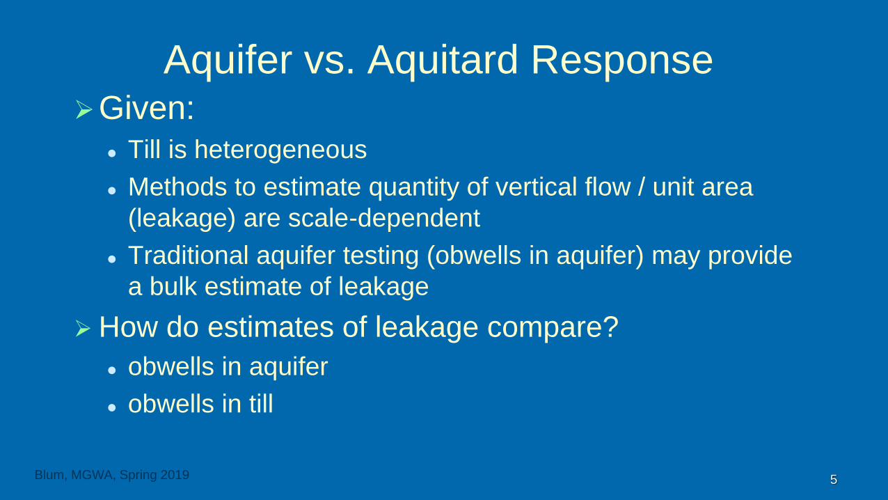
Aquifer vs. Aquitard Response➢Given:
⚫ Till is heterogeneous
⚫ Methods to estimate quantity of vertical flow / unit area
(leakage) are scale-dependent
⚫ Traditional aquifer testing (obwells in aquifer) may provide
a bulk estimate of leakage
➢How do estimates of leakage compare?
⚫ obwells in aquifer
⚫ obwells in till
5Blum, MGWA, Spring 2019

Why Leakage Matters in Layered Systems
⚫ “All layered systems are leaky”
⚫ Ultimate source of water in the system
⚫ Theis conceptual model assumes no leakage; this is a
problem
⚫ Understanding requires conceptual model that includes
leakage
Blum, MGWA, Spring 2019 6

Conceptual Model, Assumed Source of Water
Reference Source of Water
⚫ Theis (1935) - Transient change in (∆) storage only | no leakage
constant head boundary: r → ∞
⚫ de Glee (1930) - Steady-state no ∆ storage | leakage only
constant head boundary: water table
⚫ Composite (Transient & Steady-state) ∆ storage + leakage, const. head boundaries
• Hantush-Jacob (1955) ∆ storage in aquifer, no ∆ storage in aquitard
• Neuman-Witherspoon (1969) ∆ storage in both: aquifer & aquitard
Blum, MGWA, Spring 2019 7
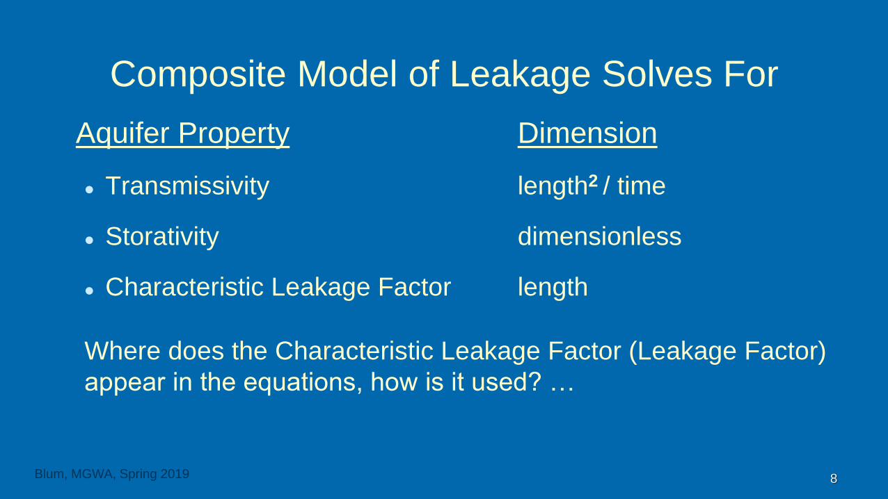
Composite Model of Leakage Solves For
Aquifer Property Dimension
⚫ Transmissivity length2 / time
⚫ Storativity dimensionless
⚫ Characteristic Leakage Factor length
Where does the Characteristic Leakage Factor (Leakage Factor)
appear in the equations, how is it used? …
Blum, MGWA, Spring 2019 8

Theis (1935) → Hantush-Jacob (1955)
Two → Three Aquifer Properties
Transmissivity
Storativity
Leakage Factor
Blum, MGWA, Spring 2019 9
Aquitard
k’ - vertical conductivity
b’ - thickness
Theis (1935) Well function, W(u)
& dimensionless parameter: r/L
Theis (1935) Storativity
unchanged

Solve for Aquitard Vertical Conductivity, k’
Known quantities: b’, T, & L
Published equation for Leakage Factor:
Aquitard hydraulic resistance, c = = time-1
Bulk Aquitard Vertical Conductivity,
Blum, MGWA, Spring 2019 10
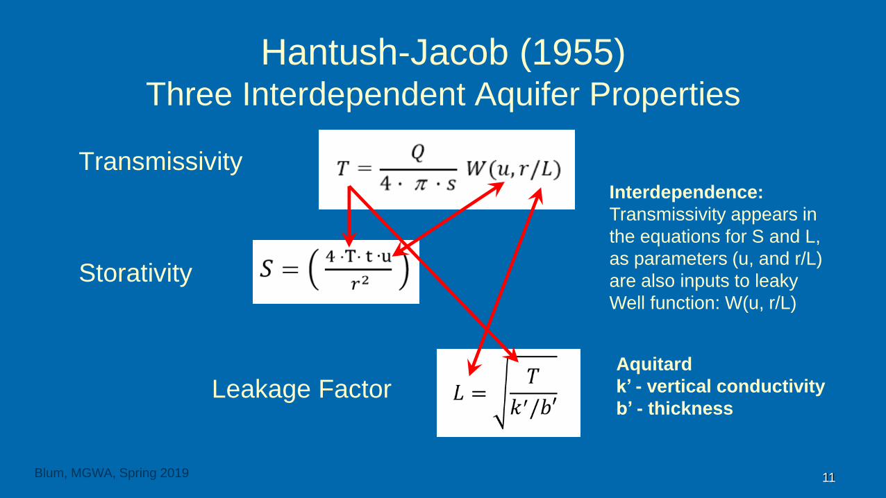
Hantush-Jacob (1955) Three Interdependent Aquifer Properties
Transmissivity
Storativity
Leakage Factor
Blum, MGWA, Spring 2019 11
Aquitard
k’ - vertical conductivity
b’ - thickness
Interdependence:
Transmissivity appears in
the equations for S and L,
as parameters (u, and r/L)
are also inputs to leaky
Well function: W(u, r/L)

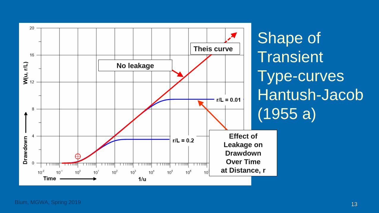
Shape of
Transient
Type-curves
Hantush-Jacob
(1955 a)
∆ Storage in
Aquifer only,
No ∆ Storage in
Aquitard
12Blum, MGWA, Spring 2019
Theis curve
Shape of
Transient
Type-curves
Hantush-Jacob
(1955 a)
No leakage
Effect of
Leakage on
Drawdown
Over Time
at Distance, r
13Blum, MGWA, Spring 2019
Theis curve
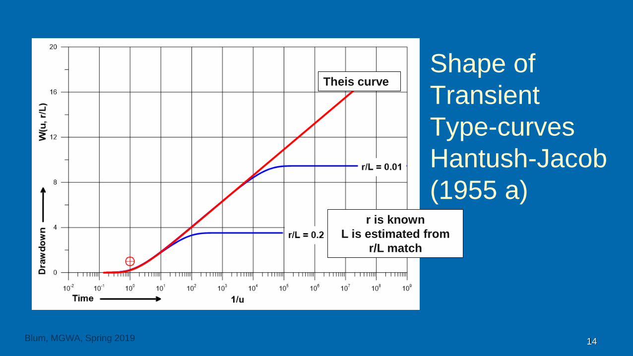
Shape of
Transient
Type-curves
Hantush-Jacob
(1955 a)r is known
L is estimated from
r/L match
14
Theis curve
Blum, MGWA, Spring 2019

Transient
Analysis
Shape
No leakage
15
Theis curve
Blum, MGWA, Spring 2019
Leaky Curve
MatchT = 2,420 ft2/day
S = 5.0e-5
r = 100 ft.
L = r / (r/L)
L = 1,430 feet

Shape of
Steady-state
Type-Curve
Hantush-Jacob
(1955 b)
Bessel function of
the second kind zero
order, Ko(x)
16Blum, MGWA, Spring 2019

Shape of
Steady-state
Type-Curve
Hantush-Jacob
(1955 b)
17Blum, MGWA, Spring 2019
log-linear within the distance
0.2 * X of pumped well
asymptotic to the X-axis
MS Excel function:
BESSELK(x,0)

Steady-state
Analysis
ShapeT = 2,330 ft2/day
S = 9.6e-4
X (s=0) = 2,340 feet
L = 2,340 / 1.12
L = 2,090 feet
18Blum, MGWA, Spring 2019
pumped well
obwell 1
obwell 2
L = X-intercept / 1.12
“Radius of Influence”
L slightly smaller
Than X-intercept,
Where drawdown = 0

Leakage Factor vs. % of Pumped Volume
Blum, MGWA, Spring 2019 19
“Radius of Influence”
Has a Problem
Zhou (2011) Sources of water,
travel times and protection areas
for wells in semi-confined
aquifers. Hydrogeology Journal
19, 1285–1291.
DOI: 10.1007/s10040-011-0762-x
Drawdown, s ~ 0

Leakage Factor vs. “Radius of Detection”
Blum, MGWA, Spring 2019 20
Working definition:
s ~ 0 at 1.12 * L
Radius of Detection
~ 30 to 50 % of pumping
induced leakage occurs
farther than the distance at
which there is measurable
drawdown
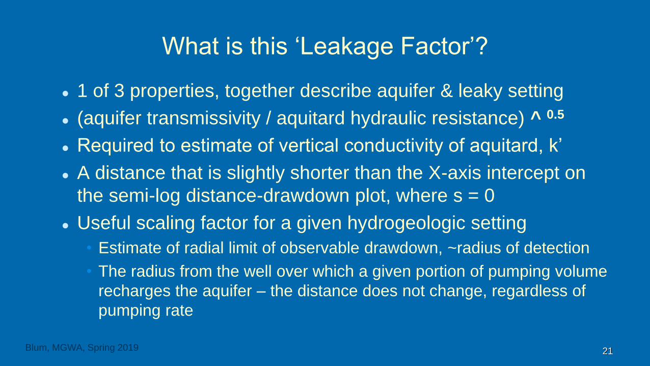
What is this ‘Leakage Factor’?
⚫ 1 of 3 properties, together describe aquifer & leaky setting
⚫ (aquifer transmissivity / aquitard hydraulic resistance) ^ 0.5
⚫ Required to estimate of vertical conductivity of aquitard, k’
⚫ A distance that is slightly shorter than the X-axis intercept on
the semi-log distance-drawdown plot, where s = 0
⚫ Useful scaling factor for a given hydrogeologic setting
• Estimate of radial limit of observable drawdown, ~radius of detection
• The radius from the well over which a given portion of pumping volume
recharges the aquifer – the distance does not change, regardless of
pumping rate
Blum, MGWA, Spring 2019 21

Has Leakage
Given You
Brain Cramp?
22Blum, MGWA, Spring 2019

Description
of Four
Aquifer
Tests
23
UM Field Camp
Cromwell
Litchfield
Olivia
Blum, MGWA, Spring 2019

Practical Concerns: Water Levels in Till
➢Can a reliable signal in till obwells develop within time-
frame of traditional one to five-day constant-rate test?
⚫ Evaluate signal reliability
Individual - obwell response is log-linear over time?
Aggregate - nest (till thickness / drawdown) is linear?
⚫ Evaluate effective thickness of till
Is response linear over the full or partial thickness of till?
24Blum, MGWA, Spring 2019

Analysis Process
➢Characterize aquifer properties (Theis & Hantush-Jacob)
➢ Verify
⚫ Drawdown in aquifer at till nest, estimate if necessary
⚫ Transient response of each till obwell is log-linear
➢ Estimate effective thickness of till
➢Model till obwell data with Aqtesolv, Neuman-
Witherspoon solution
25Blum, MGWA, Spring 2019

Cromwell
Location
26
UM Field Camp
Cromwell
Litchfield
Olivia
Blum, MGWA, Spring 2019

Cromwell
Test Site
27
Nest 1
Nest 2
Pumped Well, Cromwell 4
Blum, MGWA, Spring 2019

Cromwell
Test Site
28
Nest 1
Nest 2
~50 feet
Blum, MGWA, Spring 2019
~140 feet

Cromwell
Aquifer
Setting
Sandy
Superior
Lobe Till
29
Layer 1
Layer 2
Layer 3
Blum, MGWA, Spring 2019
Nest 2Nest 1

Cromwell
Aquifer Test
30
Well is Partially
Penetrating:
40 ft. Screen over
~145 ft. Aquifer
Thickness
Blum, MGWA, Spring 2019
Nest 2Nest 1
145 feet40 ft.
Screen

Cromwell
Aquifer Test
31
Nest 2
Four Till Obwells,
No Obwell in
Aquifer
Blum, MGWA, Spring 2019
Nest 2Nest 1
130 feet
145 feet

Cromwell
Aquifer Test
32
Nest 1
Obwell in Aquifer &
Aquitard
Blum, MGWA, Spring 2019
Nest 2Nest 1
130 feet
145 feet

Cromwell
Aquifer Test
33
Question:
What is drawdown
at top of aquifer -
base of till at
Nest 2 ?
Blum, MGWA, Spring 2019
s = ???
Nest 2Nest 1

Cromwell
Nest 2
Drawdown
at Top of
Aquifer
34Blum, MGWA, Spring 2019
5.3 feet

Cromwell Comparison
Method WellTransmissivity
T (ft2/day)
Storativity
S
Leakage
Factor
L (feet)
Vertical
Hydraulic
Conductivity
k’ (ft/day)
Aqtesolv Hantush-
Jacob
Aquifer
USGS 1-B4,380* 7.8e-3 330 2.6
Top of
Aquifer2,190
Aqtesolv Neuman-
WitherspoonTill - Nest 1 2,200 5.0e-4 590 0.83
Aqtesolv Neuman-
Witherspoon
Till - USGS
1-A & 2-E1,590 5.5e-2 224 4.1
35
* Anisotropy kz/kr = 0.5
Blum, MGWA, Spring 2019
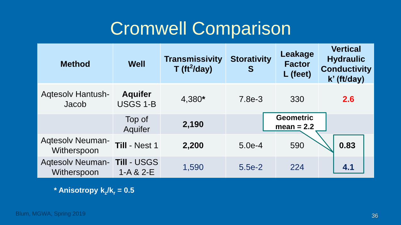
Cromwell Comparison
Method WellTransmissivity
T (ft2/day)
Storativity
S
Leakage
Factor
L (feet)
Vertical
Hydraulic
Conductivity
k’ (ft/day)
Aqtesolv Hantush-
Jacob
Aquifer
USGS 1-B4,380* 7.8e-3 330 2.6
Top of
Aquifer2,190
Aqtesolv Neuman-
WitherspoonTill - Nest 1 2,200 5.0e-4 590 0.83
Aqtesolv Neuman-
Witherspoon
Till - USGS
1-A & 2-E1,590 5.5e-2 224 4.1
36
* Anisotropy kz/kr = 0.5
Blum, MGWA, Spring 2019
Geometric
mean = 2.2

Litchfield
Location
37
UM Field Camp
Cromwell
Litchfield
Olivia
Blum, MGWA, Spring 2019

Litchfield
Test Site
38
Pumped Well
Litchfield 2
Nest 1
Nest 2
Blum, MGWA, Spring 2019

Litchfield
Aquifer
Setting
Heavy Clay
Till,
Weathered
in Places
Layer 1
Layer 2
Layer 3
39Blum, MGWA, Spring 2019
130
to
113
feet
110
feet
Nest 1

Short-
Term Test
Effects of
Pumping
Only Seen
in Till at
Nest 1
40
Unweathered -
No response
Nest 1
Nest 2
Weathered -
Responded
to pumping
Blum, MGWA, Spring 2019

Litchfield
Analysis of Short-Term Test
Method WellTransmissivity
T (ft2/day)
Storativity
S
Leakage
Factor
L (feet)
Vertical
Hydraulic
Conductivity
k’ (ft/day)
Manual
Theis t/r2
Aquifer
MW
(607417)
9,350 1.6e-4 NA NA
Manual
Hantush-Jacob
Aquifer
All9,170 2.0e-4 24,100 0.0018*
41
* Assumed till thickness of 113 feet, full thickness at Nest 1 site
Blum, MGWA, Spring 2019

Litchfield
Nest 1
Short-
Term Test
Non-linear
Response
in Till…
42Blum, MGWA, Spring 2019
Effective Thickness ?
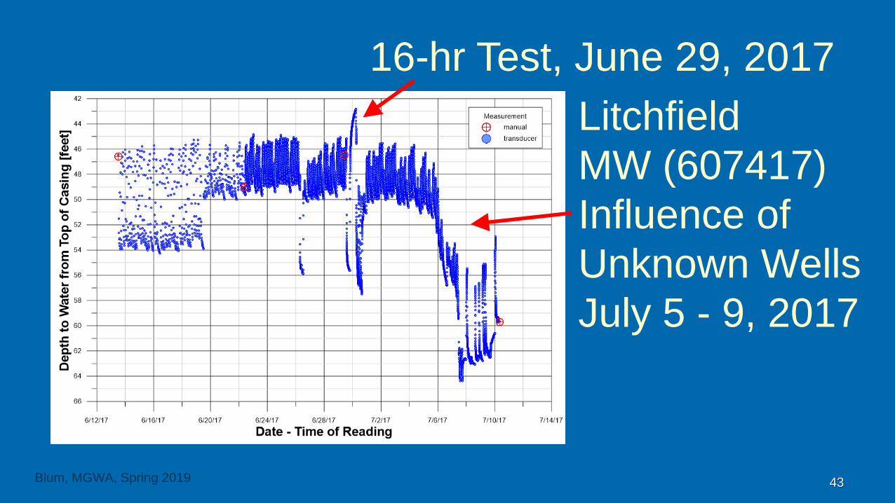
Litchfield
MW (607417)
Influence of
Unknown Wells
July 5 - 9, 2017
43Blum, MGWA, Spring 2019
16-hr Test, June 29, 2017

Litchfield
Linear
Response
in Till from
Pumping of
Unknown
Well(s)
44Blum, MGWA, Spring 2019
Effective Thickness 48 ft.

Litchfield
Impact of
Regional
Irrigation
Pumping
During
2016
45Blum, MGWA, Spring 2019
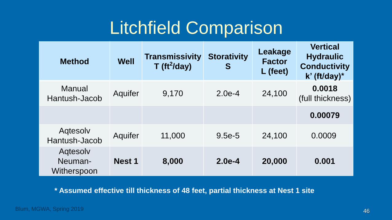
Litchfield Comparison
Method WellTransmissivity
T (ft2/day)
Storativity
S
Leakage
Factor
L (feet)
Vertical
Hydraulic
Conductivity
k’ (ft/day)*
Manual
Hantush-JacobAquifer 9,170 2.0e-4 24,100
0.0018
(full thickness)
0.00079
Aqtesolv
Hantush-JacobAquifer 11,000 9.5e-5 24,100 0.0009
Aqtesolv
Neuman-
Witherspoon
Nest 1 8,000 2.0e-4 20,000 0.001
46
* Assumed effective till thickness of 48 feet, partial thickness at Nest 1 site
Blum, MGWA, Spring 2019

Hydrogeology
Field
Camp
Location
47
UM Field Camp
Cromwell
Litchfield
Olivia
Blum, MGWA, Spring 2019
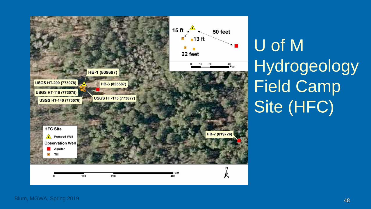
U of M
Hydrogeology
Field Camp
Site (HFC)
48Blum, MGWA, Spring 2019

HFC Schematic
Cross-Section
49
Layer 1 – water table
Layer 2 – sandy till
Layer 3 - aquifer
Blum, MGWA, Spring 2019
130 ft.
14 ft.

HFC Schematic
Cross-Section
50
Till Heterogeneity,
Local Sand
Interlayer with
Limited Extent
Blum, MGWA, Spring 2019
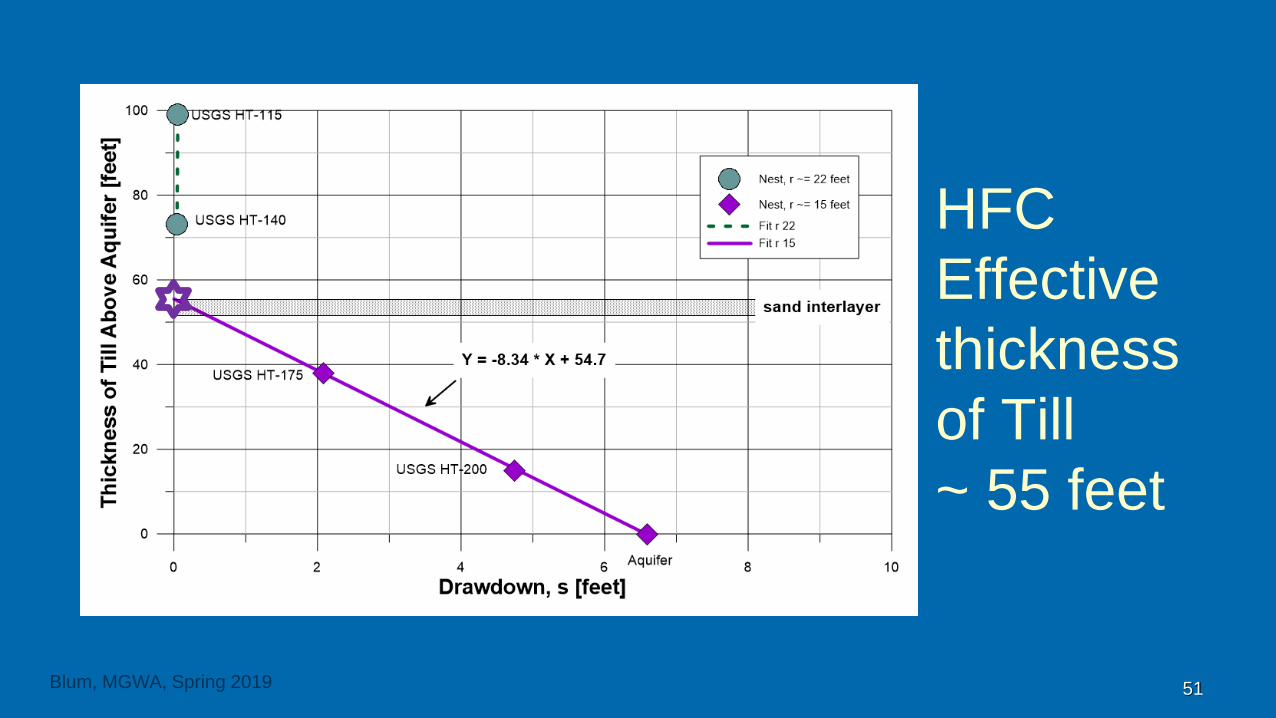
HFC
Effective
thickness
of Till
~ 55 feet
51Blum, MGWA, Spring 2019

HFC Comparison
Method WellTransmissivity
T (ft2/day)
Storativity
S
Leakage
Factor
L (feet)
Vertical
Hydraulic
Conductivity
k’ (ft/day)
Manual Hantush-
JacobAquifer 1, 380 7.3e-4 2,630 0.023
Aqtesolv Hantush-
JacobAquifer 1,360 5.8e-5 2,330 0.029
Aqtesolv Neuman-
WitherspoonAquifer 1,340 5.8e-5 2,350 0.027
Aqtesolv Neuman-
Witherspoon
Till
Obwell1,430 6.9e-4 2,770 0.0093*
52
* Assumed till thickness of 55 feet, partial thickness deep till obwells
Blum, MGWA, Spring 2019

Olivia
Location
53
UM Field Camp
Cromwell
Litchfield
Olivia
Blum, MGWA, Spring 2019

Olivia Test
Site
140 ft.
Heavy Clay
Till &
Lacustrine
Sediments
54Blum, MGWA, Spring 2019
Obwell
nest
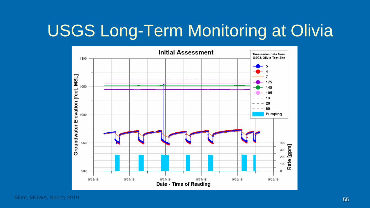
USGS Long-Term Monitoring at Olivia
55Blum, MGWA, Spring 2019
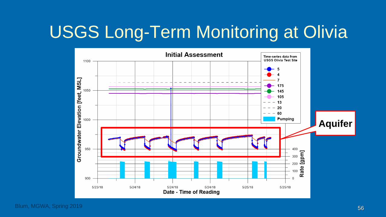
USGS Long-Term Monitoring at Olivia
56
Aquifer
Blum, MGWA, Spring 2019

USGS Long-Term Monitoring at Olivia
57
Aquitard
Blum, MGWA, Spring 2019
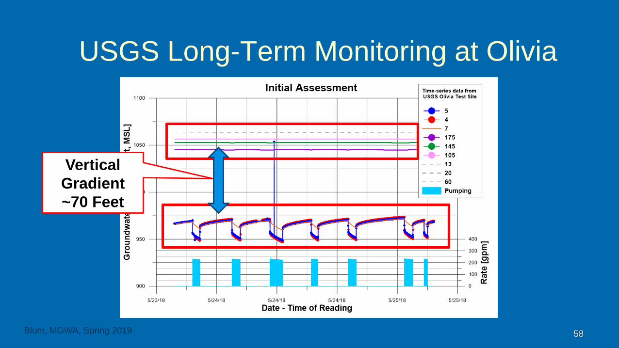
USGS Long-Term Monitoring at Olivia
58
Vertical
Gradient
~70 Feet
Blum, MGWA, Spring 2019

Olivia
Aquifer
Obwell
Response
vs.
Pumping
59Blum, MGWA, Spring 2019

Olivia
Till Obwell
Response
vs.
Pumping
60
Poro-elastic
Response
Blum, MGWA, Spring 2019

Olivia
Comparison
Actual and
Unbounded
(Ideal)
Aquifer
Response
61
Observed
Ideal
infinite
aquifer
Blum, MGWA, Spring 2019
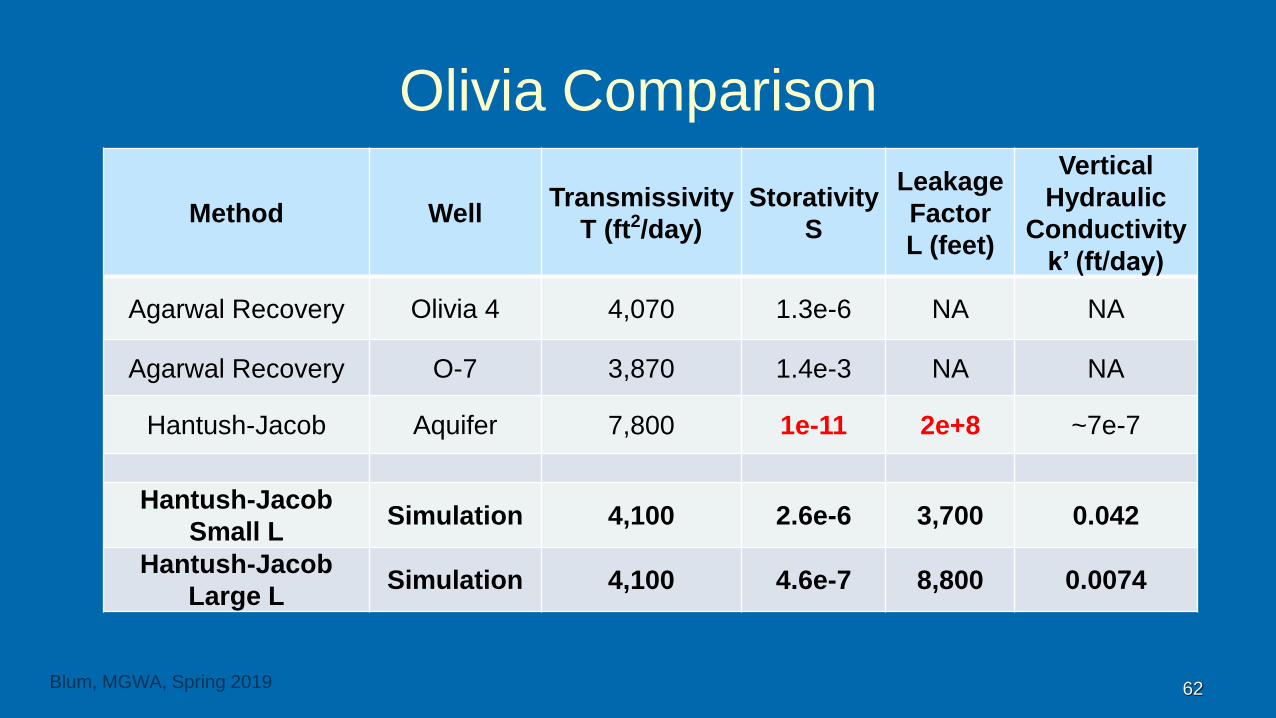
Olivia Comparison
Method WellTransmissivity
T (ft2/day)
Storativity
S
Leakage
Factor
L (feet)
Vertical
Hydraulic
Conductivity
k’ (ft/day)
Agarwal Recovery Olivia 4 4,070 1.3e-6 NA NA
Agarwal Recovery O-7 3,870 1.4e-3 NA NA
Hantush-Jacob Aquifer 7,800 1e-11 2e+8 ~7e-7
Hantush-Jacob
Small LSimulation 4,100 2.6e-6 3,700 0.042
Hantush-Jacob
Large LSimulation 4,100 4.6e-7 8,800 0.0074
62Blum, MGWA, Spring 2019

Comparison - Four Sites
63
* (x) Effective till thickness used for k’, ** Estimated properties of unbounded aquifer
Blum, MGWA, Spring 2019
SiteTransmissivity
T (ft2/day)
Storativity
S
Leakage
Factor
L (feet)
Till
Thickness
b’ (feet)
Range in
Vertical Hydraulic
Conductivity
k’(ft/day)
Cromwell 4,380 7.3e-4 550 130 0.83 to 4.1
Hydrogeology
Field Camp1,430 6.9e-4 2,770 130 (55)* 0.0093* to 0.029
Litchfield 9,000 9.5e-5 24,000 113 (48)*< 0.0008 to 0.0018
0.0009*
Olivia** ~ 4,100 ~ 1.0e-6 ~ 5,940 140 < 0.016

Conclusions - Test Methods
➢ Two different measures of vertical conductivity, k’⚫ Bulk k’ from the aquifer response
⚫ Local k’ from till obwell response (Neuman-Witherspoon)
➢Heterogeneous till complicates the comparison of k’ types⚫ Bulk k’ bias to high value - large-scale till heterogeneity within ~1.5 L
radial distance from the pumped well (Cromwell, Litchfield)
⚫ HFC nest disturbed by local heterogeneity, but the aquifer bulk and till
nest k’ (unexpectedly) nearly same value
⚫ Olivia was a null result because of bounded aquifer and lack of
appropriate conceptual model to deal with observed response in till
64Blum, MGWA, Spring 2019

General Conclusions
➢ L and k’ from aquifer tests strongly influenced by most highly
conductive till
➢ Where obwells showed a response
⚫ Site-specific Nest k’ consistent with aquifer bulk k’
⚫ Similar k’ from different methods: Hantush-Jacob, Neuman-Witherspoon
⚫ k’ range was within +/- 0.5 of geometric mean – within the typical range of
variability of aquifer k from aquifer testing
➢ Lithology of till matters (sandy till vs. heavy clay-till)
⚫ Vertical flow is ‘focused’ at the heavy clay-till sites
⚫ The flux in or out of the aquifer (recharge/discharge) is determined by the
most highly conductive areas of aquitard
65Blum, MGWA, Spring 2019
Questions & Implications
➢ How to protect drinking water from contamination in settings with
focused recharge?
➢ From these investigations, additional information about aquitards
is needed for improved models
➢ To start, methods to distinguish till settings & types of till & would
be quite helpful to focus additional data collection (testing, etc.)
⚫ Weathered / Unweathered
⚫ % Clay / % Sand
⚫ Vertical gradient across till
66Blum, MGWA, Spring 2019
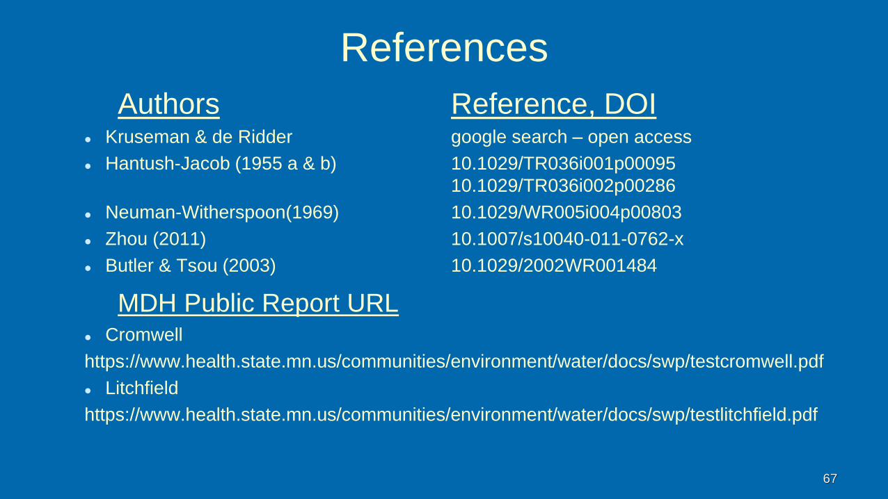
References
Authors Reference, DOI⚫ Kruseman & de Ridder google search – open access
⚫ Hantush-Jacob (1955 a & b) 10.1029/TR036i001p00095
10.1029/TR036i002p00286
⚫ Neuman-Witherspoon(1969) 10.1029/WR005i004p00803
⚫ Zhou (2011) 10.1007/s10040-011-0762-x
⚫ Butler & Tsou (2003) 10.1029/2002WR001484
MDH Public Report URL⚫ Cromwell
https://www.health.state.mn.us/communities/environment/water/docs/swp/testcromwell.pdf
⚫ Litchfield
https://www.health.state.mn.us/communities/environment/water/docs/swp/testlitchfield.pdf
67

Litchfield
MW (607417)
Influence of
Unknown Wells
July 5 - 9, 2017
68Blum, MGWA, Spring 2019
16-hr Test, June 29, 2017

Litchfield
Pervasive
Effect on
Wells in
Aquifer,
Drawdown
8 to 9 Feet
69Blum, MGWA, Spring 2019
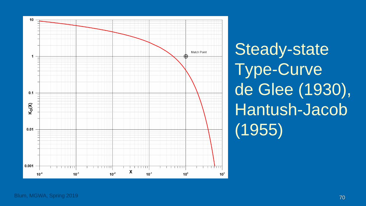
Steady-state
Type-Curve
de Glee (1930),
Hantush-Jacob
(1955)
70Blum, MGWA, Spring 2019

Steady-State Well Curve, de Glee (1930)
Different Q
Shifts Curve
on Y-axis Only
71
s
rBlum, MGWA, Spring 2019

Litchfield
Hypothetical
Well to be
Modeled
72
Nest 1
Litchfield 2
Modeled Well
r = 8,000 feet
T= 9,000 ft2/day
L= 22,000
Q = ???? gpm
Blum, MGWA, Spring 2019
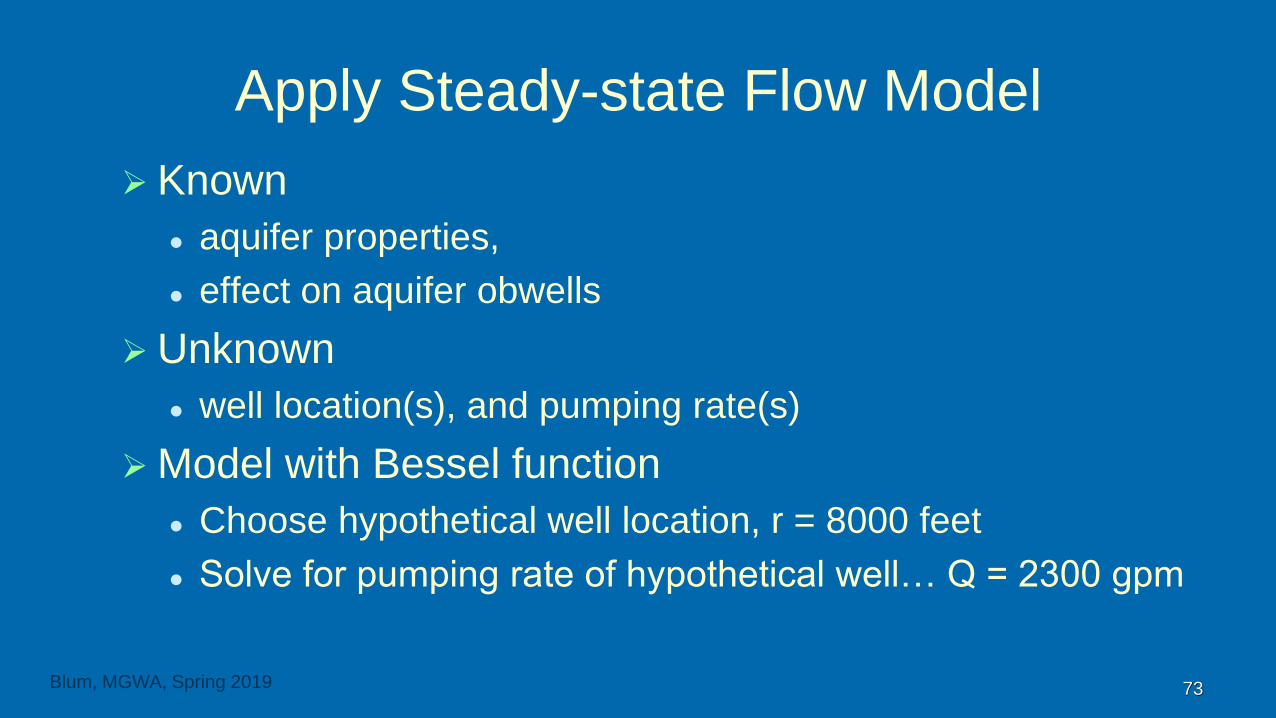
Apply Steady-state Flow Model
➢ Known
⚫ aquifer properties,
⚫ effect on aquifer obwells
➢Unknown
⚫ well location(s), and pumping rate(s)
➢Model with Bessel function
⚫ Choose hypothetical well location, r = 8000 feet
⚫ Solve for pumping rate of hypothetical well… Q = 2300 gpm
73Blum, MGWA, Spring 2019
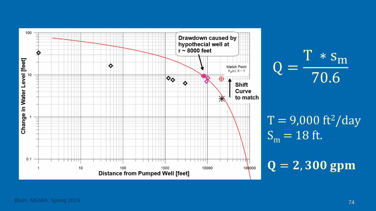
T = 9,000 ft2/daySm = 18 ft.
𝐐 = 𝟐, 𝟑𝟎𝟎 𝐠𝐩𝐦
74Blum, MGWA, Spring 2019
Q =T ∗ sm70.6