LDA + DMFT (QMC) Lectures 1, 2 &...
40
SMR.1667 - 3 Summer School and Miniconference on Dynamical Mean-Field Theory for Correlated Electrons: Applications to Real Materials, Extensions and Perspectives 25 July - 3 August, 2005 LDA + DMFT (QMC) Lectures 1, 2 & 3 Karsten Held Max-Planck-Institut fur Festkorperforschung Heisenbergstrasse 1 D-70569 Stuttgart Germany These are preliminary lecture notes, intended only for distribution to participants
Transcript of LDA + DMFT (QMC) Lectures 1, 2 &...

SMR.1667 - 3
Summer School and Miniconference on Dynamical Mean-Field Theory for Correlated Electrons:
Applications to Real Materials, Extensions and Perspectives 25 July - 3 August, 2005
LDA + DMFT (QMC) Lectures 1, 2 & 3
Karsten Held Max-Planck-Institut fur Festkorperforschung
Heisenbergstrasse 1 D-70569 Stuttgart
Germany
These are preliminary lecture notes, intended only for distribution to participants

Psi-k Newsletter #56, 65 (2003) [psi-k.dl.ac.uk/newsletters/News 56/Highlight 56.pdf]
9 SCIENTIFIC HIGHLIGHT OF THE MONTH
Realistic investigations of correlated
electron systems with LDA+DMFT
K. Held1, I. A. Nekrasov2, G. Keller3, V. Eyert4, N. Blumer5, A. K. McMahan6,
R. T. Scalettar7, Th. Pruschke3, V. I. Anisimov2, and D. Vollhardt3
1 Max-Planck Institute for Solid State Research, D-70569 Stuttgart, Germany2 Institute of Metal Physics, Russian Academy of Sciences-Ural Division,
Yekaterinburg GSP-170, Russia3 Theoretical Physics III, Center for Electronic Correlations and Magnetism,
Institute for Physics, University of Augsburg, D-86135 Augsburg, Germany4 Institute for Physics, Theoretical Physics II, University of Augsburg, D-86135 Augsburg,
Germany5 Institute for Physics, Johannes Gutenberg University, D-55099 Mainz, Germany
6 Lawrence Livermore National Laboratory, University of California, Livermore, CA 94550,
USA7 Physics Department, University of California, Davis, CA 95616, USA
Abstract
Conventional band structure calculations in the local density approximation (LDA)1–3 are
highly successful for many materials, but miss important aspects of the physics and energetics
of strongly correlated electron systems, such as transition metal oxides and f -electron sys-
tems displaying, e.g., Mott insulating and heavy quasiparticle behavior. In this respect, the
LDA+DMFT approach which merges LDA with a modern many-body approach, the dynam-
ical mean-field theory (DMFT) has proved to be a breakthrough for the realistic modeling of
correlated materials. Depending on the strength of the electronic correlation, a LDA+DMFT
calculation yields the weakly correlated LDA results, a strongly correlated metal, or a Mott
insulator. In this paper, the basic ideas and the set-up of the LDA+DMFT(X) approach,
where X is the method used to solve the DMFT equations, are discussed. Results obtained
with X=QMC (quantum Monte Carlo) and X=NCA (non-crossing approximation) are pre-
sented and compared, showing that the method X matters quantitatively. We also discuss
LDA+DMFT results for two prime examples of correlated materials, i.e., V2O3 and Ce which
undergo a Mott-Hubbard metal-insulator and volume collapse transition, respectively.
65

Table of contents
1. Introduction . . . . . . . . . . . . . . . . . . . . . . . . . . . . . . . . . . . . . . . . . . . . . . . . . . . . . . . . . . . . . . . . . . . . . . . . . . . 66
2. The LDA+DMFT approach . . . . . . . . . . . . . . . . . . . . . . . . . . . . . . . . . . . . . . . . . . . . . . . . . . . . . . . . . . . 68
2.1. Ab initio electronic Hamiltonian . . . . . . . . . . . . . . . . . . . . . . . . . . . . . . . . . . . . . . . . . . . . . . . . . . 68
2.2. Density functional theory . . . . . . . . . . . . . . . . . . . . . . . . . . . . . . . . . . . . . . . . . . . . . . . . . . . . . . . . . 69
2.3. Local density approximation . . . . . . . . . . . . . . . . . . . . . . . . . . . . . . . . . . . . . . . . . . . . . . . . . . . . . . 70
2.4. Supplementing LDA with local Coulomb correlations . . . . . . . . . . . . . . . . . . . . . . . . . . . . . . 71
2.5. Dynamical mean-field theory. . . . . . . . . . . . . . . . . . . . . . . . . . . . . . . . . . . . . . . . . . . . . . . . . . . . . . 73
2.6. QMC method to solve DMFT. . . . . . . . . . . . . . . . . . . . . . . . . . . . . . . . . . . . . . . . . . . . . . . . . . . . . 76
2.7. NCA method to solve DMFT . . . . . . . . . . . . . . . . . . . . . . . . . . . . . . . . . . . . . . . . . . . . . . . . . . . . . 79
2.8. Simplifications for transition metal oxides with well separated eg- and t2g-bands . . . 81
3. Extensions and alternatives . . . . . . . . . . . . . . . . . . . . . . . . . . . . . . . . . . . . . . . . . . . . . . . . . . . . . . . . . . . . 82
3.1. Self-consistent LDA+DMFT . . . . . . . . . . . . . . . . . . . . . . . . . . . . . . . . . . . . . . . . . . . . . . . . . . . . . . 82
3.2. LDA+DMFT as a spectral density functional theory . . . . . . . . . . . . . . . . . . . . . . . . . . . . . . 82
3.3. LDA+cluster DMFT. . . . . . . . . . . . . . . . . . . . . . . . . . . . . . . . . . . . . . . . . . . . . . . . . . . . . . . . . . . . . . 83
3.4. GW+DMFT. . . . . . . . . . . . . . . . . . . . . . . . . . . . . . . . . . . . . . . . . . . . . . . . . . . . . . . . . . . . . . . . . . . . . . 83
4. Comparison of different methods to solve DMFT . . . . . . . . . . . . . . . . . . . . . . . . . . . . . . . . . . . . . . . 84
5. Mott-Hubbard metal-insulator transition in V2O3 . . . . . . . . . . . . . . . . . . . . . . . . . . . . . . . . . . . . . . 87
6. The Cerium volume collapse . . . . . . . . . . . . . . . . . . . . . . . . . . . . . . . . . . . . . . . . . . . . . . . . . . . . . . . . . . . 91
7. Conclusion and Outlook . . . . . . . . . . . . . . . . . . . . . . . . . . . . . . . . . . . . . . . . . . . . . . . . . . . . . . . . . . . . . . . 96
1 Introduction
One of the most important challenges of theoretical solid state physics is the development of
tools for the accurate calculation of material properties. In this respect, density functional
theory (DFT) within the local density approximation (LDA)1–3 turned out to be unexpectedly
successful, and established itself as the method for realistic solid state calculations in the last
century. This is surprising because LDA is a serious approximation to the Coulomb interac-
tion between electrons. In particular the correlation but also the exchange contribution of the
Coulomb interaction is only treated rudimentarily, i.e., by means of a local density and by a
functional obtained from the jellium model, a weakly correlated problem. The success of LDA
shows, however, that this treatment is sufficient for many materials, both for calculating ground
state energies and bandstructures, implying that electronic correlations are rather weak in these
materials. However, there are important classes of materials where LDA fails, such as transition
metal oxides or heavy fermion systems, i.e., materials where electronic correlations are strong.
For example, LDA predicts La2CuO4 and V2O3, to be metals4,5 whereas, in reality, they are
insulators. The physics of these Mott insulators is dominated by the formation of Hubbard
bands, an effect of electronic correlations which splits the LDA bands into two sets of bands,
separated by a local Coulomb repulsion U . Such Mott insulating behavior occurs already in the
paramagnetic phase, with magnetic order setting in at lower temperatures. The Mott physics
and the associated energy gain is completely missing in the LDA. It can, however, be described
by the LDA+U method, at least for ordered systems. But, the energy gain due to the formation
of Hubbard bands is so large in LDA+U that for realistic values of U it almost automatically
yields split bands and (ordered) insulating behavior, even if this is not correct. The reason for
this is that the energy of the correlated metal is strongly overestimated. Hence, LDA+U is a
66

������������������������������������������������������������������������������������������������������������
������������������������������������������������������������������������������������������������������������
������������������������������������������������������������������������������������������������������������
������������������������������������������������������������������������������������������������������������
LDA LDA+DMFT LDA+U
0 U/W ∞metal insulator
Figure 1: With increasing strength of the local Coulomb repulsion U (relative to the LDA band-
width W ), one observes a weakly correlated metal (left density of states), a strongly correlated
metal with a quasiparticle peak at the Fermi energy (middle), and a Mott insulator (right). The
weakly correlated metal and the (ordered) Mott insulator are correctly described by LDA and
LDA+U, respectively. LDA+DMFT gives the correct answer for all values of U and subsumes
the LDA valid for small U/W and the LDA+U results for the Mott insulator appearing at large
U/W .
good method for describing Mott insulators, but not for calculating strongly correlated metals
or systems in the vicinity of a Mott-Hubbard metal-insulator transition. Missing in both LDA
and LDA+U is the quasiparticle physics, which even at a rather large Coulomb interaction U
(or at U =∞ with a non-integer number of interacting electrons per site) still gives a metallic
behavior determined by quasiparticles with a larger effective mass than the LDA electrons. This
mass enhancement ranges from a moderate increase in many transition metal oxides to the high
effective masses observed in 4f -based heavy fermion compounds. LDA and also LDA+U fail to
account for this kind of physics and the associated Kondo-like energy scale gained in comparison
with the Mott insulator.
LDA+DMFT does not only include the correct quasiparticle physics and the corresponding en-
ergetics but, at the same time, reproduces the LDA and LDA+U results in the limits where
these methods are valid, see Fig. 1. For weakly correlated systems, we know that LDA provides
the correct description, as does the LDA+DMFT approach which gives the same results as
LDA if the local Coulomb interaction U is small. On the other hand, LDA+DMFT agrees with
the LDA+U results for symmetry-broken Mott insulators at large Coulomb interaction U . In
addition, however, LDA+DMFT also describes the correlated metals occurring either at some-
what smaller Coulomb interactions U or when Mott insulators are doped. Thus, LDA+DMFT
provides the correct physics for all Coulomb interactions and dopings, whereas LDA yields an
uncorrelated metal even if the material at hand is a strongly-correlated metal or a Mott insula-
tor. Similarly, LDA+U yields an insulator for the ab-initio-calculated U -values of 3d transition
metal oxides, even for materials which should be metallic.
67

With the ability of LDA+DMFT to describe the full range of materials from weakly to strongly
correlated metals to Mott insulators, it is not astonishing that it has proved to be a break-
through for the calculation of correlated materials. Since more and more physicists from the
bandstructure and many-body communities show interest in this novel method, we would like to
present here, as a ψk scientific highlight of the month, an introduction to LDA+DMFT. We also
present results for two of the most famous strongly-correlated materials, i.e., the transition metal
oxide V2O3 which is the prime example of a system undergoing a Mott-Hubbard metal-insulator
transition, and the 4f -electron system Ce with its volume collapse transition. The presentation
is following in many parts the conference proceedings Ref. 6, also see the conference proceedings
Refs. 7.
In Section 2 the LDA+DMFT approach is presented, starting with the ab initio electronic
Hamiltonian in Section 2.1, continuing with DFT in Section 2.2, LDA in Section 2.3, the con-
struction of a model Hamiltonian in Section 2.4, and DMFT in Section 2.5. As methods used
to solve the DMFT we discuss the quantum Monte Carlo (QMC) algorithm in Section 2.6 and
the non-crossing approximation (NCA) in Section 2.7. A simplified treatment for transition
metal oxides is introduced in Section 2.8. Extensions and alternatives to the LDA+DMFT ap-
proach are discussed, focusing on a self-consistent LDA+DMFT scheme in Section 3.1, spectral
density functional theory in Section 3.2, cluster extensions of DMFT in Section 3.3, and the
GW+DMFT approach in Section 3.4. As a particular example, the LDA+DMFT calculation
for La1−xSrxTiO3 is discussed in Section 4, emphasizing that the method X to solve the DMFT
matters on a quantitative level. Our calculations for the Mott-Hubbard metal-insulator tran-
sition in V2O3 are presented in Section 5, in comparison to the experiment. Section 6 reviews
our recent calculations of the Ce α-γ transition, in the perspective of the models referred to as
Kondo volume collapse and Mott transition scenario. A summary of the LDA+DMFT set-up
and applications followed by a discussion of future prospects closes the presentation in Section 7.
2 The LDA+DMFT approach
2.1 Ab initio electronic Hamiltonian
Within Born-Oppenheimer approximation8 and neglecting relativistic effects, electronic proper-
ties of solid state systems are described by the electronic Hamiltonian
H =∑
σ
∫d3r Ψ+(r, σ)
[− ~2
2me∆ + Vion(r)
]Ψ(r, σ)
+1
2
∑
σσ′
∫d3r d3r′ Ψ+(r, σ)Ψ+(r′, σ′) Vee(r−r′) Ψ(r′, σ′)Ψ(r, σ). (1)
Here, Ψ+(r, σ) and Ψ(r, σ) are field operators that create and annihilate an electron at position
r with spin σ, ∆ is the Laplace operator, me the electron mass, e the electron charge, and
Vion(r) = −e2∑
i
Zi|r−Ri|
and Vee(r−r′) =e2
2
∑
r6=r′
1
|r− r′| (2)
68

denote the one-particle ionic potential of all ions i with charge eZi at given positions Ri, and
the electron-electron interaction, respectively.
While the ab initio Hamiltonian (1) is easy to write down it is impossible to solve it exactly
if more than a few electrons are involved. Numerical methods like Green’s Function Monte
Carlo and related approaches have been used successfully for relatively modest numbers of
electrons. Even so, however, the focus of the work has been on jellium and on light atoms and
molecules like H, H2, 3He, 4He with only a few electrons. Because of this, one has to make
substantial approximations to deal with the Hamiltonian (1) like the LDA approximation or the
LDA+DMFT approach which is the subject of the present paper.
2.2 Density functional theory
The fundamental theorem of DFT by Hohenberg and Kohn1 (see, e.g., the review by Jones and
Gunnarsson3) states that the ground state energy is a functional of the electron density which
assumes its minimum at the electron density of the ground state. Following Levy,9 this theorem
is easily proved and the functional even constructed by taking the minimum (infimum) of the
energy expectation value w.r.t. all (many-body) wave functions ϕ(r1σ1, ... rNσN ) at a given
electron number N which yield the electron density ρ(r):
E[ρ] = inf{〈ϕ|H |ϕ〉
∣∣∣ 〈ϕ|N∑
i=1
δ(r − ri)|ϕ〉 = ρ(r)}. (3)
However, this construction is of no practical value since it actually requires the evaluation of
the Hamiltonian (1). Only certain contributions like the Hartree energy, i.e., EHartree[ρ] =12
∫d3r′ d3r Vee(r−r′) ρ(r′)ρ(r), and the energy of the ionic potential Eion[ρ] =
∫d3r Vion(r) ρ(r)
can be expressed directly in terms of the electron density. This leads to
E[ρ] = Ekin[ρ] +Eion[ρ] +EHartree[ρ] +Exc[ρ], (4)
where Ekin[ρ] denotes the kinetic energy, and Exc[ρ] is the unknown exchange and correlation
term which contains the energy of the electron-electron interaction except for the Hartree term.
Hence all the difficulties of the many-body problem have been transferred into Exc[ρ]. Instead
of minimizing E[ρ] with respect to ρ one minimizes it w.r.t. a set of one-particle wave functions
ϕi related to ρ via
ρ(r) =N∑
i=1
|ϕi(r)|2. (5)
To guarantee the normalization of ϕi, the Lagrange parameters εi are introduced such that the
variation δ{E[ρ] + εi[1−∫d3r|ϕi(r)|2]}/δϕi(r) = 0 yields the Kohn-Sham2 equations:
[− ~2
2me∆ + Vion(r) +
∫d3r′ Vee(r−r′)ρ(r′) +
δExc[ρ]
δρ(r)
]ϕi(r) = εi ϕi(r). (6)
These equations have the same form as a one-particle Schrodinger equation and yield a kinetic
energy for the one-particle wave-function ansatz, i.e., Ekin[ρmin] = −∑Ni=1〈ϕi|~2∆/(2me)|ϕi〉
where ϕi denote the self-consistent (spin-degenerate) solutions of Eqs. (6) and (5) with lowest
“energy” εi. However, this kinetic energy functional gives not the true kinetic energy of the
69

First principles information:
atomic numbers, crystal structure (lattice, atomic positions)
Choose initial electronic density ρ(r)
Calculate effective potential using the LDA [Eq. (7)]
Veff(r) = Vion(r) +
∫d3r′ Vee(r− r′)ρ(r′) +
δExc[ρ]
δρ(r)
Solve Kohn-Sham equations [Eq. (6)]
[− ~
2
2m∆ + Veff(r)− εi
]ϕi(r) = 0
Calculate electronic density [Eq. (5)],
ρ(r) =
N∑
i
|ϕi(r)|2
Iterate to self-consistency
Calculate band structure εi(k) [Eq. (6)], partial and total DOS,
Hamiltonian [Eq. (11)] =⇒ LDA+DMFT, total energy E[ρ] [Eq.
(3)], . . .
Figure 2: Flow diagram of the DFT/LDA calculations.
correlated problem which would require that the exact δExc also comprises the difference. Also
note, that the one-particle potential of Eq. (6), i.e.,
Veff(r) = Vion(r) +
∫d3r′ Vee(r−r′)ρ(r′) +
δExc[ρ]
δρ(r), (7)
is only an auxiliary potential which artificially arises in the approach to minimize E[ρ]. Thus,
the wave functions ϕi and the Lagrange parameters εi have no physical meaning at this point.
Altogether, these equations allow for the DFT/LDA calculation, see the flow diagram Fig. 2.
2.3 Local density approximation
So far no approximations have been employed since the difficulty of the many-body problem was
only transferred to the unknown functional Exc[ρ]. For this term the local density approximation
(LDA) which approximates the functional Exc[ρ] by a function that depends on the local density
only, i.e.,
Exc[ρ]→∫d3r ELDA
xc (ρ(r)), (8)
was found to be unexpectedly successful. Here, ELDAxc (ρ(r)) is usually calculated from the
perturbative solution10 or the numerical simulation11 of the jellium problem which is defined by
70

Vion(r) = const.
In principle, DFT/LDA only allows one to calculate static properties like the ground state
energy or its derivatives. However, one of the major applications of LDA is the calculation of
band structures. To this end, the Lagrange parameters εi are interpreted as the physical (one-
particle) energies of the system under consideration. Since the true ground-state is not a simple
one-particle wave-function, this is an approximation beyond DFT. Actually, this approximation
corresponds to the replacement of the Hamiltonian (1) by
HLDA =∑
σ
∫d3r Ψ+(r, σ)
[−~2
2me∆ + Vion(r) +
∫d3r′ Vee(r−r′)ρ(r′) +
δELDAxc [ρ]
δρ(r)
]Ψ(r, σ).(9)
For practical calculations one needs to expand the field operators w.r.t. a basis Φilm, e.g., a
linearized muffin-tin orbital (LMTO)12,13 basis (i denotes lattice sites; l and m are orbital
indices). In this basis,
Ψ+(r, σ) =∑
ilm
cσ†ilmΦilm(r) (10)
such that the Hamiltonian (9) reads
HLDA =∑
ilm,jl′m′,σ
(δilm,jl′m′ εilm nσilm + tilm,jl′m′ cσ†ilmc
σjl′m′). (11)
Here, nσilm = cσ†ilmcσilm,
tilm,jl′m′ =⟨
Φilm
∣∣∣− ~2∆
2me+ Vion(r) +
∫d3r′Vee(r−r′)ρ(r′) +
δELDAxc [ρ]
δρ(r)
∣∣∣Φjl′m′⟩
(12)
for ilm 6= jl′m′ and zero otherwise; εilm denotes the corresponding diagonal part.
As for static properties, the LDA approach based on the self-consistent solution of Hamiltonian
(11) together with the calculation of the electronic density Eq. (5) [see the flow diagram Fig. 2]
has also been highly successful for band structure calculations – but only for weakly correlated
materials.3 It is not reliable when applied to correlated materials and can even be completely
wrong because it treats electronic correlations only very rudimentarily.
2.4 Supplementing LDA with local Coulomb correlations
Of prime importance for correlated materials are the local Coulomb interactions between d-
and f -electrons on the same lattice site since these contributions are largest. This is due to
the extensive overlap (w.r.t. the Coulomb interaction) of these localized orbitals which results in
strong correlations. Moreover, the largest non-local contribution is the nearest-neighbor density-
density interaction which, to leading order in the number of nearest-neighbor sites, yields only
the Hartree term (see Ref. 14 and, also, Ref. 15) which is already included in the LDA. To take
the local Coulomb interactions into account, one can supplement the LDA Hamiltonian (11)
with the local Coulomb matrix approximated by the (most important) matrix elements U σσ′mm′
(Coulomb repulsion and Z-component of Hund’s rule coupling) and Jmm′ (spin-flip terms of
Hund’s rule coupling) between the localized electrons (for which we assume i = id and l = ld):
H = HLDA +1
2
∑
i=id,l=ld
∑
mσ,m′σ′
′Uσσ
′mm′ nilmσnilm′σ′
71

������������
������������
n−1 n+1
E
n
Figure 3: Left: In the constrained LDA calculation the interacting d- or f -electrons on one
lattice site are kinetically decoupled from the rest of the system, i.e., they cannot hop to other
lattice sites or to other orbitals. By contrast, the non-interacting electrons can still still hop
to other sites (indicated by dashed lines). Right: This allows one to constrain the number n
of interacting d- or f -electrons on the decoupled site and to calculate the corresponding LDA
energies E(n) (circles); the dashed line sketches the behavior of HLDA defined in Eq. (11).
−1
2
∑
i=id,l=ld
∑
mσ,m′
′Jmm′ c
†ilmσ c
†ilm′σ cilm′σ cilmσ −
∑
i=id,l=ld
∑
mσ
∆εd nilmσ. (13)
Here, the prime on the sum indicates that at least two of the indices of an operator have to
be different, and σ =↓ (↑) for σ =↑ (↓). In principle, also a pair hopping term of the form12
∑i=id,l=ld
∑mσ,m′′ Jmm′ c
†ilmσ c
†ilmσ cilm′σ cilm′σ would occur in Eq. (13). This term has not yet
been included in LDA+DMFT calculations because one commonly assumes that configurations
where one orbital is doubly occupied while another is empty are rare if the Hund’s exchange
and the hopping terms are included. In typical applications we have U ↑↓mm ≡ U , Jmm′ ≡ J ,
Uσσ′
mm′ = U−2J−Jδσσ′ for m 6= m′ (here, the first term 2J is due to the reduced Coulomb repul-
sion between different orbitals and the second term Jδσσ′ directly arises from the Z-component
of Hund’s rule coupling). With the number of interacting orbitals M , the average Coulomb
interaction is then
U =U + (M − 1)(U − 2J) + (M − 1)(U − 3J)
2M − 1. (14)
The last term of the Hamiltonian (13) reflects a shift of the one-particle potential of the inter-
acting orbitals and is necessary if the Coulomb interaction is taken into account. This last term
led to some criticism and we would, thus, like to discuss the origin of this term in more detail
below.
The calculation of the local Coulomb interaction U , or similarly the Hund’s exchange constant
J , is not at all trivial and requires additional approximations. Presently, the best method
available which takes into account screening effects is the constrained LDA method.16 The basic
idea of constrained LDA is to perform LDA calculations for a slightly modified problem, i.e.,
a problem where the interacting d- or f -electrons of one site are kinetically decoupled from
the rest of the system, i.e., their hopping matrix elements tildm,jlm′ are set to zero, see Fig. 3.
This allows one to change the number of interacting electrons on this site. At the same time
screening effects of the other electrons, which are redistributed if the number of d- or f -electrons
72

is changed on the decoupled site, are taken into account. In a LDA+DMFT calculation, one
expects an average number nd of interacting electrons per site on average; typically nd is close
to an integer number. Then, one can do constrained LDA calculations for n− 1, n, and n + 1
electrons on the decoupled site, leading to three corresponding total energies, see Fig. 3. The
LDA Hamiltonian HLDA which was calculated at a fixed density ρ(r) would predict a linear
change of the LDA energy with the number of interacting electrons, i.e., E(nd) = E0 + εLDAd nd
with εLDAd = dELDA/dnd. This does not take into account the Coulomb interaction U which
requires a higher energy cost to add the (n+ 1)th electron than to add the nth electron. This
effect leads to the curvature in Fig. 3 and is taken into account in the Hamiltonian (13) which
yields E(n) = E0 + (1/2) Und(nd − 1) + (εLDAd + ∆εd)nd. Note, that part of ∆εd just arises to
cancel the Coulomb contribution (1/2) d[U nd(nd − 1)]/dnd = U(nd − 1/2). We can, therefore,
determine U and ∆εd by fitting these parameters to reproduce the constrained LDA energies.
That is, we require that Hamiltonian (13) correctly reproduces the LDA energy for three different
numbers of interacting electrons on the decoupled site. Similarly, the Hund’s exchange J can
be calculated by constrained LDA calculations with the spin polarization. One should keep in
mind that, while the total LDA spectrum is rather insensitive to the choice of the basis, the
constrained LDA calculations of U strongly depends on the shape of the orbitals which are
considered to be interacting. E.g., for LaTiO3 at a Wigner Seitz radius of 2.37 a.u. for Ti a
LMTO-ASA calculation17 using the TB-LMTO-ASA code12 yielded U = 4.2 eV in comparison
to the value U = 3.2 eV calculated by ASA-LMTO within orthogonal representation.18 Thus,
an appropriate basis is mandatory and, even so, a significant uncertainty in U remains.
In the following, it is convenient to work in reciprocal space where the matrix elements of H0LDA,
i.e., the LDA one-particle energies without the local Coulomb interaction, are given by
(H0LDA(k))qlm,q′l′m′ = (HLDA(k))qlm,q′l′m′ − δqlm,q′l′m′δql,qdld∆εdnd. (15)
Here, q is an index of the atom in the primitive cell, (HLDA(k))qlm,q′l′m′ is the matrix element
of (11) in k-space, and qd denotes the atoms with interacting orbitals in the primitive cell.
The non-interacting part, H0LDA, supplemented with the local Coulomb interaction forms the
(approximated) ab initio Hamiltonian for a particular material under investigation:
H = H0LDA +
1
2
∑
i=id,l=ld
∑
mσ,m′σ′
′Uσσ
′mm′ nilmσnilm′σ′
−1
2
∑
i=id,l=ld
∑
mσ,m′
′Jmm′ c
†ilmσ c
†ilm′σ cilm′σ cilmσ . (16)
2.5 Dynamical mean-field theory
The many-body extension of LDA, Eq. (16), was proposed by Anisimov et al.19 in the con-
text of their LDA+U approach. Within LDA+U the Coulomb interactions of (16) are treated
within the Hartree-Fock approximation. Hence, LDA+U does not contain true many-body
physics. While this approach is successful in describing long-range ordered, insulating states of
correlated electronic systems it fails to describe strongly correlated paramagnetic states. To go
beyond LDA+U and capture the many-body nature of the electron-electron interaction, i.e., the
frequency dependence of the self energy, various approximation schemes have been proposed and
73

lm
12
DMFT
Σ (ω)σ
Figure 4: If the number of neighboring lattice sites goes to infinity, the central limit theorem
holds and fluctuations from site-to-site can be neglected. This means that the influence of these
neighboring sites can be replaced by a mean influence, the dynamical mean-field described by
the self energy Σσlm(ω). This DMFT problem is equivalent to the self-consistent solution of
the k-integrated Dyson equation (19) and the multi-band Anderson impurity model Eq. (18).
Similar in nature are the coherent potential approximation (CPA) for disorder and the Weiss
mean-field theory for spin systems. Indeed, DMFT reduces to these approximations if there is
disorder and no Coulomb interaction or if the electrons can be described effectively as localized
spins, respectively.
applied recently.20–25 One of the most promising approaches, first implemented by Anisimov et
al.,20 is to solve (16) within DMFT14,26–33 (”LDA+DMFT”). Of all extensions of LDA only the
LDA+DMFT approach is presently able to describe the physics of strongly correlated, param-
agnetic metals with well-developed upper and lower Hubbard bands and a narrow quasiparticle
peak at the Fermi level. This characteristic three-peak structure is a signature of the importance
of many-body effects.29,30
During the last ten years, DMFT has proved to be a successful approach for investigating
strongly correlated systems with local Coulomb interactions.33 It becomes exact in the limit of
high lattice coordination numbers or dimension d, i.e., it is controlled in 1/d,14,26 and preserves
the dynamics of local interactions. Hence, it represents a dynamical mean-field approximation.
In this non-perturbative approach the lattice problem is mapped onto an effective single-site
problem (see Fig. 4) which has to be determined self-consistently together with the k-integrated
Dyson equation connecting the self energy Σ and the on-site (or in cell) Green function G at
frequency ω:
Gqlm,q′l′m′(ω) =1
VB
∫d3k
([ω1 + µ1−H0
LDA(k)− Σ(ω)]−1)qlm,q′l′m′
. (17)
Here, 1 is the unit matrix, µ the chemical potential, the matrix H 0LDA(k) is defined in (15), Σ(ω)
denotes the self energy matrix which is non-zero only between the interacting orbitals, [...]−1
implies the inversion of the matrix with elements n (=qlm), n′(=q′l′m′), and the integration
extends over the Brillouin zone with volume VB.
The DMFT single-site problem depends on (the Weiss field) G(ω)−1 = G(ω)−1 + Σ(ω) and is
equivalent29,30 to an Anderson impurity model (the history and the physics of this model is sum-
marized by Anderson in Ref. 34) if its hybridization ∆(ω) satisfies G−1(ω) = ω−∫dω′∆(ω′)/(ω−
ω′). The local one-particle Green function at a Matsubara frequency iων = i(2ν + 1)π/β (β:
inverse temperature), orbital index m (l = ld, q = qd), and spin σ is given by the following
functional integral over Grassmann variables ψ and ψ∗ (for an introduction to anti-commuting
74

Choose an initial self energy Σ
Iterate with Σ=Σnew until convergence, i.e. ||Σ− Σnew|| < ε
Calculate G from Σ via the k-integrated Dyson Eq. (17):
Gqlm,q′l′m′(ω) =1
VB
∫d3k
([ω1 + µ1−H0
LDA(k)− Σ(ω)]−1)qlm,q′l′m′
G = (G−1 + Σ)−1
Calculate G from G via the DMFT single-site problem Eq. (18)
Gσνm = − 1
Z
∫D[ψ]D[ψ∗]ψσνmψ
σ∗νme
A[ψ,ψ∗,G−1]
Σnew = G−1 −G−1
Figure 5: Flow diagram of the DMFT self-consistency cycle.
Grassmann variables see Ref. 35):
Gσνm = − 1
Z
∫D[ψ]D[ψ∗]ψσνmψ
σ∗νme
A[ψ,ψ∗,G−1]. (18)
Here, Z =∫D[ψ]D[ψ∗]ψσνmψ
σ∗νm exp(A[ψ,ψ∗,G−1]) is the partition function and the single-site
action A has the form (the interaction part of A is in terms of the “imaginary time” τ , i.e., the
Fourier transform of ων)
A[ψ,ψ∗,G−1] =∑
ν,σ,m
ψσ∗νm(Gσνm)−1ψσνm
−1
2
∑
mσ,mσ′
′Uσσ
′mm′
β∫
0
dτ ψσ∗m (τ)ψσm (τ)ψσ′∗m′ (τ)ψσ
′m′ (τ)
+1
2
∑
mσ,m
′Jmm′
β∫
0
dτ ψσ∗m (τ)ψσm(τ)ψσ∗m′(τ)ψσm′(τ) . (19)
This single-site problem (18) has to be solved self-consistently together with the k-integrated
Dyson equation (17) to obtain the DMFT solution of a given problem, see the flow diagram
Fig. 5.
Due to the equivalence of the DMFT single-site problem and the Anderson impurity problem a
variety of approximate techniques have been employed to solve the DMFT equations, such as the
iterated perturbation theory (IPT)29,33 and the non-crossing approximation (NCA),36–38 as well
as numerical techniques like quantum Monte Carlo simulations (QMC),39–42 exact diagonaliza-
tion (ED),33,43 or numerical renormalization group (NRG).44 QMC and NCA will be discussed
75

in more detail in Section 2.6 and 2.7, respectively. IPT is non-self-consistent second-order per-
turbation theory in U for the Anderson impurity problem (18) at half filling. It represents an
ansatz that also yields the correct perturbational U 2-term and the correct atomic limit for the
self energy off half filling,45 for further details see Refs. 20, 21, 45. ED directly diagonalizes the
Anderson impurity problem at a limited number of lattice sites and orbitals. NRG first replaces
the conduction band by a discrete set of states at DΛ−n (D: bandwidth; n = 0, ...,Ns) and then
diagonalizes this problem iteratively with increasing accuracy at low energies, i.e., with increas-
ing Ns. In principle, QMC and ED are exact methods, but they require an extrapolation, i.e.,
the discretization of the imaginary time ∆τ → 0 (QMC) or the number of lattice sites of the
respective impurity model Ns →∞ (ED), respectively.
In the context of LDA+DMFT we refer to the computational schemes to solve the DMFT
equations discussed above as LDA+DMFT(X) where X=IPT,20 NCA,25 QMC17 have been
investigated in the case of La1−xSrxTiO3. The same strategy was formulated by Lichten-
stein and Katsnelson21 as one of their LDA++ approaches. Lichtenstein and Katsnelson ap-
plied LDA+DMFT(IPT),46 and were the first to use LDA+DMFT(QMC),47 to investigate
the spectral properties of iron. Recently, among others V2O3,48,49 Ca(Sr)VO3,50 LiV2O4,51
Ca2−xSrxRuO4,52,53 CrO2,54 Ni,55 Fe,55 Mn,56 Pu,57,58 and Ce59–61 have been studied by
LDA+DMFT. Realistic investigations of itinerant ferromagnets (e.g., Ni) have also recently
become possible by combining density functional theory with multi-band Gutzwiller wave func-
tions.62
2.6 QMC method to solve DMFT
The self-consistency cycle of the DMFT (Fig. 5) requires a method to solve for the dynamics of
the single-site problem of DMFT, i.e., Eq. (18). The QMC algorithm by Hirsch and Fye39 is a
well established method to find a numerically exact solution for the Anderson impurity model
and allows one to calculate the impurity Green function G at a given G−1 as well as correlation
functions. In essence, the QMC technique maps the interacting electron problem Eq. (18)
onto a sum of non-interacting problems where the single particle moves in a fluctuating, time-
dependent field and evaluates this sum by Monte Carlo sampling, see the flow diagram Fig. 6 for
an overview. To this end, the imaginary time interval [0, β] of the functional integral Eq. (18)
is discretized into Λ steps of size ∆τ = β/Λ, yielding support points τl = l∆τ with l = 1 . . .Λ.
Using this Trotter discretization, the integral∫ β
0 dτ is transformed to the sum∑Λ
l=1 ∆τ and the
exponential terms in Eq. (18) can be separated via the Trotter-Suzuki formula for operators A
and B63
e−β(A+B) =
Λ∏
l=1
e−∆τAe−∆τB +O(∆τ), (20)
which is exact in the limit ∆τ → 0. The single site action A of Eq. (19) can now be written in
the discrete, imaginary time as
A[ψ,ψ∗,G−1] = ∆τ2Λ−1∑
σm l,l′=0
ψσml∗Gσm−1(l∆τ − l′∆τ)ψσml′
76

−1
2∆τ∑′
mσ,m′σ′Uσσ
′mm′
Λ−1∑
l=0
ψσml∗ψσmlψ
σ′m′l∗ψσ′m′l, (21)
where the first term was Fourier-transformed from Matsubara frequencies to imaginary time.
In a second step, the M(2M − 1) interaction terms in the single site action A are decoupled by
introducing a classical auxiliary field sσσ′
lmm′ :
exp
{∆τ
2Uσσ
′mm′(ψ
σml∗ψσml − ψσ
′m′l∗ψσ′m′l)
2
}=
1
2
∑
sσσ′
lmm′ =±1
exp{
∆τλσσ′
lmm′sσσ′lmm′(ψ
σml∗ψσml − ψσ
′m′l∗ψσ′m′l)
}, (22)
where cosh(λσσ′
lmm′) = exp(∆τUσσ′mm′/2) and M is the number of interacting orbitals. This so-
called discrete Hirsch-Fye-Hubbard-Stratonovich transformation can be applied to the Coulomb
repulsion as well as the Z-component of Hund’s rule coupling.64 It replaces the interacting
system by a sum of ΛM(2M − 1) auxiliary fields sσσ′
lmm′ . The functional integral can now be
solved by a simple Gauss integration because the Fermion operators only enter quadratically,
i.e., for a given configuration s = {sσσ′lmm′} of the auxiliary fields the system is non-interacting.
The quantum mechanical problem is then reduced to a matrix problem
Gσml1l2 =1
Z1
2
∑
l
′∑
m′σ′,m′′σ′′
∑
sσ′′σ′lm′′m′ =±1
[(M σs
m )−1]l1l2
∏
mσ
det Mσsm (23)
with the partition function Z, the matrix
Mσsm = ∆τ2[Gσ
m−1 + Σσ
m]e−λσsm + 1− e−λσs
m (24)
and the elements of the matrix λσsm
λσsmll′ = −δll′
∑
m′σ′λσσ
′mm′ σ
σσ′mm′s
σσ′lmm′ . (25)
Here σσσ′
mm′ = 2Θ(σ′− σ+ δσσ′ [m′−m]− 1) changes sign if (mσ) and (m′σ′) are exchanged. For
more details, e.g., for a derivation of Eq. (24) for the matrix M, see Refs. 33, 39.
Since the sum in Eq. (23) consists of 2ΛM(2M−1) addends, a complete summation for large Λ is
computationally impossible. Therefore the Monte Carlo method, which is often an efficient way
to calculate high-dimensional sums and integrals, is employed for importance sampling of Eq.
(23). In this method, the integrand F (x) is split up into a normalized probability distribution
P and the remaining term O:
∫dxF (x) =
∫dxO(x)P (x) ≡ 〈O〉P (26)
with ∫dxP (x) = 1 and P (x) ≥ 0. (27)
In statistical physics, the Boltzmann distribution is often a good choice for the function P :
P (x) =1
Z exp(−βE(x)). (28)
77

Choose random auxiliary field configuration s = {sσσ′lmm′}
Calculate the current Green function Gcur from Eq. (30)
(Gcur)σml1l2 =
[(M σs
m )−1]l1l2
with M from Eq. (24) and the input Gσm(ων)−1 = Gσm(ων)−1 + Σσm(ων).
Do NWU times (warm up sweeps)
MC-sweep (Gcur, s)
Do NMC times (measurement sweeps)
MC-sweep (Gcur, s)
G = G + Gcur/NMC
Figure 6: Flow diagram of the QMC algorithm to calculate the Green function matrix G using
the procedure MC-sweep of Fig. 7.
For the sum of Eq. (23), this probability distribution translates to
P (s) =1
Z∏
mσ
det Mσsm (29)
with the remaining term
O(s)σml1l2 =[(M σs
m )−1]l1l2
. (30)
Instead of summing over all possible configurations, the Monte Carlo simulation generates con-
figurations xi according to the probability distribution P (x) and averages the observable O(x)
over these xi. Therefore the relevant parts of the phase space with a large Boltzmann weight
are taken into account to a greater extent than the ones with a small weight, coining the name
importance sampling for this method. With the central limit theorem one gets forN statistically
independent addends the estimate
〈O〉P =1
NN∑
xi∈P (x)i=1
O(xi)±1√N
√〈O2〉P − 〈O〉2P . (31)
Here, the error and with it the number of needed addends N is nearly independent of the di-
mension of the integral. The computational effort for the Monte Carlo method is therefore only
rising polynomially with the dimension of the integral and not exponentially as in a normal inte-
gration. Using a Markov process and single spin-flips in the auxiliary fields, the computational
cost of the algorithm in leading order of Λ is
2aM(2M − 1)Λ3 × number of MC-sweeps, (32)
where a is the acceptance rate for a single spin-flip.
78

Choose M(2M − 1)Λ times a set (l mm′ σ σ′),
define snew to be s except for the element sσσ′
lmm′ which has opposite sign.
Calculate flip probability Ps→snew = min{1, P (snew)/P (s)} with
P (snew)/P (s) =∏
mσ
det Mσsnewm /
∏
mσ
det Mσsm
and M from Eq. (24).`````````````````````
�������������
Random number ∈ (0, 1) < Ps→snew ?
yes no
s = snew; recalculate Gcur via Eq. (30) Keep s
Figure 7: Procedure MC-sweep using the Metropolis65 rule to change the sign of sσσ′
lmm′ . The
recalculation of Gcur, i.e., the matrix M of Eq. (24), simplifies to O(Λ2) operations if only one
sσσ′
lmm′ changes sign.33,39
The advantage of the QMC method (for the algorithm see the flow diagram Fig. 6) is that it
is (numerically) exact. It allows one to calculate the one-particle Green function as well as
two-particle (or higher) Green functions. On present workstations the QMC approach is able
to deal with up to seven interacting orbitals and temperatures above about room temperature.
Very low temperatures are not accessible because the numerical effort grows like Λ3 ∝ 1/T 3 .
Since the QMC approach calculates G(τ) or G(iωn) with a statistical error, it also requires the
maximum entropy method66 to obtain the Green function G(ω) at real (physical) frequencies ω.
2.7 NCA method to solve DMFT
The NCA approach is a resolvent perturbation theory in the hybridization parameter ∆(ω) of
the effective Anderson impurity problem.36 Thus, it is reliable if the Coulomb interaction U is
large compared to the band-width and also offers a computationally inexpensive approach to
check the general spectral features in other situations.
To see how the NCA can be adapted for the DMFT, let us rewrite Eq. (17) as
Gσ(z) =1
Nk
∑
k
[z −H0LDA(k)− Σσ(z)]−1 (33)
where z = ω + i0+ + µ. Again, H0LDA(k), Σσ(z) and, hence, G0
σ(ζ) and Gσ(z) are matrices in
orbital space. Note that Σ(z) has nonzero entries for the correlated orbitals only.
On quite general grounds, Eq. (33) can be cast into the form
Gσ(z) =1
z −E0 − Σσ(z)−∆σ(z)(34)
where
E0 =1
Nk
∑
k
H0LDA(k) (35)
79

with the number of k points Nk and
limω→±∞
<e{∆σ(ω + iδ)} = 0 . (36)
Given the matrix E0, the Coulomb matrix U and the hybridization matrix ∆σ(z), we are now
in a position to set up a resolvent perturbation theory with respect to ∆σ(z). To this end, we
first have to diagonalize the local Hamiltonian
Hlocal =∑
σ
∑
qml
∑
q′m′l′c†qlmσE
0qlm,q′l′m′cqlmσ +
1
2
∑
mσ
∑
m′σ′Uσσ
′mm′nqdldmσnqdldm′σ′
−1
2
∑
mσ
∑
m′Jmm′c
†qdldmσ
c†qdldm′σcqdldm′σcqdldmσ
=∑
α
Eα|α〉〈α|
(37)
with local eigenstates |α〉 and energies Eα. In contrast to the QMC, this approach allows one
to take into account the full Coulomb matrix plus spin-orbit coupling.
With the states |α〉 defined above, the fermionic operators with quantum numbers κ = (q, l,m)
are expressed as
c†κσ =∑
α,β
(Dκσβα
)∗ |α〉〈β| ,
cκσ =∑
α,β
Dκσαβ |α〉〈β| .
(38)
The key quantity for the resolvent perturbation theory is the resolvent R(z), which obeys a
Dyson equation36
R(z) = R0(z) +R0(z)S(z)R(z) , (39)
where R0αβ(z) = 1/(z − Eα)δαβ and Sαβ(z) denotes the self energy for the local states due to
the coupling to the environment through ∆(z).
The self energy Sαβ(z) can be expressed as power series in the hybridization ∆(z).36 Retaining
only the lowest-, i.e. 2nd-order terms leads to a set of self-consistent integral equations
Sαβ(z) =∑
σ
∑
κκ′
∑
α′β′
∫dε
πf(ε) (Dκσ
α′α)∗ Γκκ′
σ (ε)Rα′β′(z + ε)Dκ′σβ′β
+∑
σ
∑
κκ′
∑
α′β′
∫dε
π(1− f(ε))Dκσ
α′αΓκκ′
σ (ε)Rα′β′(z − ε)(Dκ′σβ′β
)∗ (40)
to determine Sαβ(z), where f(ε) denotes Fermi’s function and Γ(ε) = −=m {∆(ε+ i0+)}. The
set of equations (40) is in the literature referred to as non-crossing approximation (NCA),
because, when viewed in terms of diagrams, these diagrams contain no crossing of band-electron
lines. In order to close the cycle for the DMFT, we still have to calculate the true local Green
function Gσ(z). This, however, can be done within the same approximation with the result
Gκκ′
σ (iω) =1
Zlocal
∑
α,α′
∑
ν,ν′Dκσαα′
(Dκ′σνν′
)∗ ∮ dze−βz
2πiRαν(z)Rα′ν′(z + iω) . (41)
80

Here, Zlocal =∑
α
∮dze−βz
2πiRαα(z) denotes the local partition function and β is the inverse
temperature.
Like any other technique, the NCA has its merits and disadvantages. As a self-consistent
resummation of diagrams it constitutes a conserving approximation to the Anderson impurity
model. Furthermore, it is a (computationally) fast method to obtain dynamical results for this
model and thus also within DMFT. However, the NCA is known to violate Fermi liquid properties
at temperatures much lower than the smallest energy scale of the problem and whenever charge
excitations become dominant.38,67 Hence, in some parameter ranges it fails in the most dramatic
way and must therefore be applied with considerable care.38
2.8 Simplifications for transition metal oxides with well separated eg- and
t2g-bands
Many transition metal oxides are cubic perovskites, with only a slight distortion of the cubic
crystal structure. In these systems the transition metal d-orbitals lead to strong Coulomb
interactions between the electrons. The cubic crystal-field of the oxygen causes the d-orbitals
to split into three degenerate t2g- and two degenerate eg-orbitals. This splitting is often so
strong that the t2g- or eg-bands at the Fermi energy are rather well separated from all other
bands. In this situation the low-energy physics is well described by taking only the degenerate
bands at the Fermi energy into account. Without symmetry breaking, the Green function
and the self energy of these bands remain degenerate, i.e., Gqlm,q′l′m′(z) = G(z)δqlm,q′l′m′ and
Σqlm,q′l′m′(z) = Σ(z)δqlm,q′l′m′ for l = ld and q = qd (where ld and qd denote the electrons in the
interacting band at the Fermi energy). Downfolding to a basis with these degenerate qd-ld-bands
results in an effective Hamiltonian H0 effLDA (where indices l = ld and q = qd are suppressed)
Gmm′(ω) =1
VB
∫d3k
([ω1 + µ1−H0 eff
LDA(k)− Σ(ω)]−1)mm′
. (42)
Due to the diagonal structure of the self energy the degenerate interacting Green function can
be expressed via the non-interacting Green function G0(ω):
G(ω) = G0(ω − Σ(ω)) =
∫dε
N0(ε)
ω − Σ(ω)− ε . (43)
Thus, it is possible to use the Hilbert transformation of the unperturbed LDA-calculated density
of states (DOS) N 0(ε), i.e., Eq. (43), instead of Eq. (17). This simplifies the calculations
considerably. With Eq. (43) also some conceptual simplifications arise: (i) the subtraction of∑i=id,l=ld
∑mσ ∆εd nilmσ [see Eq. (13)] only results in an (unimportant) shift of the chemical
potential in (43) and, thus, the exact form of ∆εd is irrelevant; (ii) Luttinger’s theorem of Fermi
pinning holds, i.e., the interacting DOS at the Fermi energy is fixed at the value of the non-
interacting DOS at T = 0 within a Fermi liquid; (iii) as the number of electrons within the
different bands is fixed, the LDA+DMFT approach is automatically self-consistent.
81

3 Extensions and modifications of LDA+DMFT
3.1 Self-consistent LDA+DMFT calculations
In the present form of the LDA+DMFT scheme the band-structure input due to LDA and
the inclusion of the electronic correlations by DMFT are performed as successive steps without
subsequent feedback. In general, the DMFT solution will result in a change of the occupation of
the different bands involved. This changes the electron density ρ(r) and, thus, results in a new
LDA-Hamiltonian HLDA (11) since HLDA depends on ρ(r). At the same time also the Coulomb
interaction U changes and needs to be determined by a new constrained LDA calculation. In a
self-consistent LDA+DMFT scheme, HLDA and U would define a new Hamiltonian (16) which
again needs to be solved within DMFT, etc., until convergence is reached:
6
-- -ρ(r)DMFT
HLDA, U nilm ρ(r)(44)
Without Coulomb interaction (U = 0) this scheme reduces to the self-consistent solution of the
Kohn-Sham equations. A self-consistency scheme similar to Eq. (44) was employed by Savrasov
and Kotliar58 in their calculation of Pu (without self-consistency for U). The quantitative
difference between non-self-consistent and self-consistent LDA+DMFT depends on the change
of the number of electrons in the different bands after the DMFT calculation, which of course
depends on the problem at hand. E.g., for the Ce calculation presented in Section 6, this change
was very minor in the vicinity of α-γ transition but more significant at lower volumes.
In this context, we would also like to note that an ab initio DMFT scheme formulated directly
in the continuum was recently proposed by Chitra and Kotliar.68
3.2 LDA+DMFT as a spectral density functional theory
Our derivation of the LDA+DMFT method was physically motivated. That is, we started from
the assumption that the Kohn-Sham equations, i.e., the LDA part, yield the correct results for
the weakly correlated s- or p-bands, while the DMFT-part takes into account the local Coulomb
interactions of the strongly correlated d- or f -bands. Using the effective action construction
by Fukuda et al.,69 Savrasov et al.7,57,58 embedded LDA+DMFT in a functional theory with
a functional E[Gildm(ω), ρ(r)] which depends on the electron density ρ(r) and the local Green
functionGildm(ω) (thus coining the name spectral density functional theory7). This is in the spirit
of density functional theory with the LDA+DMFT equations emerging from the minimization
of E[Gildm(ω), ρ(r)] w.r.t. Gildm(ω) and ρ(r). If the functional E[Gildm(ω), ρ(r)] were known
exactly one would obtain the exact ground state energy. However, since the exact functional is
unknown one has to introduce approximations. Then, LDA+DMFT is a workable approximation
to the spectral density function theory, similar to LDA within DFT.
82

3.3 Cluster extensions of DMFT
DMFT reliably describes local correlations in terms of the local (or, equivalently k-independent)
self energy Σildm,ildm′(ω). For some problems like, e.g., fluctuations in the vicinity of a phase
transition or the formation of a spin-singlet on two neighboring sites, non-local correlations are
important. The standard DMFT described in Section 2.5 neglects such non-local correlations
because only a single site with local correlations in an average environment (a dynamical mean-
field) is considered. However, in principle, DMFT can also treat more than one site, i.e., a cell of
sites, in an average environment. E.g., if the primitive contains several sites with interacting d-
or f -orbitals a natural choice for the DMFT cell would be this cell. Then, non-local correlations
Σildm,jldm′(ω) would be taken into account if i and j are within the cell, whereas such correlations
would be neglected if i and j are located in different cells. Furthermore, even if the primitive
contains only one interacting site one may consider a larger DMFT cell with several interacting
sites, treating non-local correlations within that cell but not between different cells. This is the
basic idea of cluster DMFT approaches.33,70–72
An alternative scheme, named dynamical cluster approximation (DCA), has been proposed by
Hettler et al.73 The DCA has the advantage of preserving the translational symmetry. While
cluster DMFT can be best understood in real space, it is instructive to go to k-space for DCA.
Within DCA the first Brillouin zone is divided into Nc patches around k-vectors K, assuming
the self energy to be constant within each patch only (in contrast to DMFT, where the self
energy is constant for all k-vectors). In real space, the DCA cluster has periodic boundary
conditions instead of open boundary conditions for the cluster DMFT scheme. In addition, the
dynamical mean-field couples to every site of the cluster, whereas within cluster DMFT it couples
exclusively to the boundary sites. Whether cluster DMFT or DCA provides a better scaling
w.r.t. cluster size Nc →∞ is still a matter of debate and likely depends on the problem at hand
(both approaches give the correct behavior of any finite-dimensional problem for Nc →∞). It is
important to note, and not a matter of course, that all these approaches70–73 lead to physically
correct (causal) Green functions.
A third route was proposed by Schiller et al.74 It is a natural extension of DMFT in the sense
that it takes into account all diagrams to next order in 1/d (d: spatial dimension), i.e., up to
order 1/d. This leads to a theory with a single-site and a two-site cluster whose Green functions
have to be subtracted.
Cluster extensions of DMFT have been applied successfully to a couple of model systems. For
example, d-wave superconductivity in the two-dimensional Hubbard model mediated by spin-
fluctuations was found.71,75 In the context of LDA+DMFT cluster extensions of DMFT are still
work in progress.
3.4 GW+DMFT
A possible alternative to LDA+DMFT is the GW+DMFT77 approach, which uses Hedin’s GW
approximation76 instead of the LDA to generate the multi-band many-body problem Eq. (16)
in Section 2.4. From a pure, theoretical point of view, GW+DMFT has the advantage of being
a fully diagrammatic approach. This allows a better understanding of what one is actually
83

calculating and is particularly appealing to the many-body community. One might consider
GW+DMFT as the minimum set of diagrams which are necessary to realistically describe cor-
related materials: It contains the Hartree and exchange diagrams together with the RPA-like
screening of the Coulomb interaction and, via DMFT, the important local diagrams leading
to the Kondo-like and Mott-insulating physics of correlated systems. However, whether these
theoretical principles can be maintained in actual calculations still needs to be seen. Problems
already arise in mere GW calculations of weakly correlated systems where Coulomb interac-
tions are (often) calculated from the (non-diagrammatic) LDA wave function instead of the
self-consistent GW wave functions. GW+DMFT calculations for real materials are still work in
progress.77
4 Comparison of different methods to solve DMFT: the model
system La1−xSrxTiO3
The stoichiometric compound LaTiO3 is a cubic perovskite with a small orthorhombic distortion
(∠ T i−O− T i ≈ 155◦)78 and is an antiferromagnetic insulator79 below TN = 125 K.80 Above
TN , or at low Sr-doping x, and neglecting the small orthorhombic distortion (i.e., considering
a cubic structure with the same volume), LaTiO3 is a strongly correlated, but otherwise simple
paramagnet with only one 3d-electron on the trivalent Ti sites. This makes the system a perfect
trial candidate for the LDA+DMFT approach.
The LDA band-structure calculation for undoped (cubic) LaTiO3 yields the DOS shown in Fig.
8 which is typical for early transition metal oxides. The oxygen bands, ranging from −8.2 eV
to −4.0 eV, are filled such that Ti has a d1 configuration. Due to the crystal- or ligand-field
splitting, the Ti 3d-bands separate into two empty eg-bands and three degenerate t2g-bands.
Since the t2g-bands at the Fermi energy are well separated also from the other bands we employ
the approximation introduced in section 2.5 which allows us to work with the LDA DOS [Eq. (43)]
instead of the full one-particle Hamiltonian H 0LDA of [Eq. (17)]. In the LDA+DMFT calculation,
Sr-doping x is taken into account by adjusting the chemical potential to yield n = 1− x = 0.94
electrons within the t2g-bands, neglecting effects of disorder and the x-dependence of the LDA
DOS (note, that LaTiO3 and SrTiO3 have a very similar band structure within LDA). There
is some uncertainty in the LDA-calculated Coulomb interaction parameter U ∼ 4 − 5 eV (for
a discussion see Ref. 17) which is here assumed to be spin- and orbital-independent. In Fig. 9,
results for the spectrum of La0.94Sr0.06TiO3 as calculated by LDA+DMFT(IPT, NCA, QMC)
for the same LDA DOS at T ≈ 1000 K and U = 4 eV are compared.17 In Ref. 17 the formerly
presented IPT20 and NCA25 spectra were recalculated to allow for a comparison at exactly the
same parameters. All three methods yield the typical features of strongly correlated metallic
paramagnets: a lower Hubbard band, a quasi-particle peak (note that IPT produces a quasi-
particle peak only below about 250K which is therefore not seen here), and an upper Hubbard
band. By contrast, within LDA the correlation-induced Hubbard bands are missing and only a
broad central quasi-particle band (actually a one-particle peak) is obtained (Fig. 8).
While the results of the three evaluation techniques of the DMFT equations (the approximations
IPT, NCA and the numerically exact method QMC) agree on a qualitative level, Fig. 9 reveals
84

−8 −4 0 4 8Energy, eV
0
1
2
3
4
Part
ial D
OS,
sta
tes/
(eV
*orb
ital)
0
5
10
15
Tot
al D
OS,
sta
tes/
eV
Figure 8: Densities of states of LaTiO3 calculated with LDA-LMTO. Upper figure: total DOS;
lower figure: partial t2g (solid lines) and eg (dashed lines) DOS [reproduced from Ref. 17].
−3 0 3 6Energy (eV)
Inte
nsity
in a
rbitr
ary
units
QMCNCAIPT
−0.3 0 0.3
LDA
−3 0 3 6
T=80K
T=1000K
Figure 9: Spectrum of La0.94Sr0.06TiO3 as calculated by LDA+DMFT(X) at T = 0.1 eV (≈1000 K) and U = 4 eV employing the approximations X=IPT, NCA, and numerically exact
QMC. Inset left: Behavior at the Fermi level including the LDA DOS. Inset right: X=IPT and
NCA spectra at T = 80 K [reproduced from Ref. 17].
85

considerable quantitative differences. In particular, the IPT quasi-particle peak found at low
temperatures (see right inset of Fig. 9) is too narrow such that it disappears already at about
250 K and is, thus, not present at T ≈ 1000 K. A similarly narrow IPT quasi-particle peak
was found in a three-band model study with Bethe-DOS by Kajueter and Kotliar.45 Besides
underestimating the Kondo temperature, IPT also produces notable deviations in the shape of
the upper Hubbard band. Although NCA comes off much better than IPT it still underestimates
the width of the quasiparticle peak by a factor of two. Furthermore, the position of the quasi-
particle peak is too close to the lower Hubbard band. In the left inset of Fig. 9, the spectra at the
Fermi level are shown. At the Fermi level, where at sufficiently low temperatures the interacting
DOS should be pinned at the non-interacting value, the NCA yields a spectral function which
is almost by a factor of two too small. The pinning of the interacting DOS mentioned above
holds for the situation here where only degenerate bands are involved and the system is a Fermi
liquid. It is due to the k-independence of the self-energy; nonetheless, the effective mass is
renormalized: m∗/m0 = 1− ∂<Σ(w)/∂ω|ω=0. The shortcomings of the NCA-results, with a too
small low-energy scale and too much broadened Hubbard bands for multi-band systems, are well
understood and related to the neglect of exchange type diagrams.82 Similarly, the deficiencies of
the IPT-results are not entirely surprising in view of the semi-phenomenological nature of this
approximation, especially for a system off half filling.
This comparison shows that the choice of the method used to solve the DMFT equations is
indeed important, and that, at least for the present system, the approximations IPT and NCA
differ quantitatively from the numerically exact QMC. Nevertheless, the NCA gives a rather
good account of the qualitative spectral features and, because it is fast and can often be applied
at comparatively low temperatures, can yield an overview of the physics.
Photoemission spectra provide a direct experimental tool to study the electronic structure and
spectral properties of electronically correlated materials. A comparison of LDA+DMFT(QMC)
at 1000 K83 with the experimental photoemission spectrum84 of La0.94Sr0.06TiO3 is presented
in Fig 10. To take into account the uncertainty in U ,17 we present results for U = 3.2, 4.25 and
5 eV. All spectra are multiplied with the Fermi step function and are Gauss-broadened with a
broadening parameter of 0.3 eV to simulate the experimental resolution.84 LDA band structure
calculations, the results of which are also presented in Fig. 10, clearly fail to reproduce the broad
band observed in the experiment at 1-2 eV below the Fermi energy.84 Taking the correlations
between the electrons into account, this lower band is easily identified as the lower Hubbard
band whose spectral weight originates from the quasi-particle band at the Fermi energy and
which increases with U . The best agreement with experiment concerning the relative intensities
of the Hubbard band and the quasi-particle peak and, also, the position of the Hubbard band
is found for U = 5 eV. The value U = 5 eV is still compatible with the ab initio calculation
of this parameter within LDA.17 One should also bear in mind that photoemission experiments
are sensitive to surface properties. Due to the reduced coordination number at the surface the
bandwidth is likely to be smaller, and the Coulomb interaction less screened, i.e., larger. Both
effects make the system more correlated and, thus, might also explain why better agreement is
found for U = 5 eV. Besides that, also the polycrystalline nature of the sample, as well as spin
and orbital85 fluctuation not taken into account in the LDA+DMFT approach, will lead to a
further reduction of the quasi-particle weight.
86
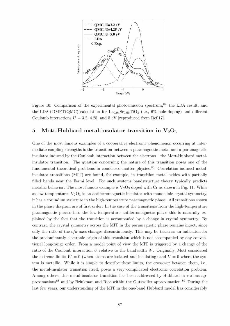
−3 −2 −1 0 1Energy (eV)
Inte
nsity
in a
rbitr
ary
units
QMC, U=3.2 eVQMC, U=4.25 eVQMC, U=5.0 eVLDAExp.
Figure 10: Comparison of the experimental photoemission spectrum,84 the LDA result, and
the LDA+DMFT(QMC) calculation for La0.94Sr0.06TiO3 (i.e., 6% hole doping) and different
Coulomb interactions U = 3.2, 4.25, and 5 eV [reproduced from Ref.17].
5 Mott-Hubbard metal-insulator transition in V2O3
One of the most famous examples of a cooperative electronic phenomenon occurring at inter-
mediate coupling strengths is the transition between a paramagnetic metal and a paramagnetic
insulator induced by the Coulomb interaction between the electrons – the Mott-Hubbard metal-
insulator transition. The question concerning the nature of this transition poses one of the
fundamental theoretical problems in condensed matter physics.86 Correlation-induced metal-
insulator transitions (MIT) are found, for example, in transition metal oxides with partially
filled bands near the Fermi level. For such systems bandstructure theory typically predicts
metallic behavior. The most famous example is V2O3 doped with Cr as shown in Fig. 11. While
at low temperatures V2O3 is an antiferromagnetic insulator with monoclinic crystal symmetry,
it has a corundum structure in the high-temperature paramagnetic phase. All transitions shown
in the phase diagram are of first order. In the case of the transitions from the high-temperature
paramagnetic phases into the low-temperature antiferromagnetic phase this is naturally ex-
plained by the fact that the transition is accompanied by a change in crystal symmetry. By
contrast, the crystal symmetry across the MIT in the paramagnetic phase remains intact, since
only the ratio of the c/a axes changes discontinuously. This may be taken as an indication for
the predominantly electronic origin of this transition which is not accompanied by any conven-
tional long-range order. From a model point of view the MIT is triggered by a change of the
ratio of the Coulomb interaction U relative to the bandwidth W . Originally, Mott considered
the extreme limits W = 0 (when atoms are isolated and insulating) and U = 0 where the sys-
tem is metallic. While it is simple to describe these limits, the crossover between them, i.e.,
the metal-insulator transition itself, poses a very complicated electronic correlation problem.
Among others, this metal-insulator transition has been addressed by Hubbard in various ap-
proximations88 and by Brinkman and Rice within the Gutzwiller approximation.89 During the
last few years, our understanding of the MIT in the one-band Hubbard model has considerably
87

(d1-d2LI ) hybridization (Uozumi et al., 1993). Cluster-model analysis has revealed considerable weight ofcharge-transfer configurations, d3LI ,d4LI 2, . . . , mixed intothe ionic d2 configuration, resulting in a net d-electronnumber of nd.3.1 (Bocquet et al., 1996). This value isconsiderably larger than the d-band filling or the formald-electron number n52 and is in good agreement withthe value (nd53.0) deduced from an analysis of core-core-valence Auger spectra (Sawatzky and Post, 1979).If the above local-cluster CI picture is relevant to experi-ment, the antibonding counterpart of the split-off bond-ing state is predicted to be observed as a satellite on thehigh-binding-energy side of the O 2p band, although itsspectral weight may be much smaller than the bondingstate [due to interference between the d2→d1
1e andd3LI →d2LI 1e photoemission channels; see Eq. (3.12)].Such a spectral feature was indeed observed in an ultra-violet photoemission study by Smith and Henrich (1988)and in a resonant photoemission study by Park andAllen (1997). In spite of the strong p-d hybridizationand the resulting charge-transfer satellite mechanism de-scribed above, it is not only convenient but also realisticto regard the d1-d2LI bonding band as an effective V 3dband (lower Hubbard band). The 3d wave function isthus considerably hybridized with oxygen p orbitals andhence has a relatively small effective U of 1–2 eV (Sa-watzky and Post, 1979) instead of the bare value U;4 eV. Therefore the effective d bandwidth W becomescomparable to the effective U : W;U . With these factsin mind, one can regard V2O3 as a model Mott-Hubbardsystem and the (degenerate) Hubbard model as a rel-evant model for analyzing the physical properties ofV2O3.
The time-honored phase diagram for doped V2O3 sys-tems, (V12xCrx)2O3 and (V12xTix)2O3 , is reproducedin Fig. 70. The phase boundary represented by the solidline is of first order, accompanied by thermal hysteresis(Kuwamoto, Honig, and Appel, 1980). In a Cr-dopedsystem (V12xCrx)2O3 , a gradual crossover is observedfrom the high-temperature paramagnetic metal (PM) to
FIG. 69. Photoemission spectra of V2O3 in the metallic phasetaken using photon energies in the 3p-3d core excitation re-gion. From Shin et al., 1990.
FIG. 68. Corundum structure of V2O3.
FIG. 70. Phase diagram for doped V2O3 systems,(V12xCrx)2O3 and (V12xTix)2O3. From McWhan et al., 1971,1973.
1147Imada, Fujimori, and Tokura: Metal-insulator transitions
Rev. Mod. Phys., Vol. 70, No. 4, October 1998
Figure 11: Experimental phase diagram of V2O3 doped with Cr and Ti [reproduced from Ref. 87].
Doping V2O3 affects the lattice constants in a similar way as applying pressure (generated either
by a hydrostatic pressure P , or by changing the V -concentration from V2O3 to V2−yO3) and
leads to a Mott-Hubbard transition between the paramagnetic insulator (PI) and metal (PM).
At lower temperatures, a Mott-Heisenberg transition between the paramagnetic metal (PM) and
the antiferromagnetic insulator (AFI) is observed.
improved, in particular due to the application of dynamical mean-field theory.90
Both the paramagnetic metal V2O3 and the paramagnetic insulator (V0.962Cr0.038)2O3 have the
same corundum crystal structure with only slightly different lattice parameters.91,92 Neverthe-
less, within LDA both phases are found to be metallic (see Fig. 12). The LDA DOS shows a
splitting of the five Vanadium d-orbitals into three t2g states near the Fermi energy and two
eσg states at higher energies. This reflects the (approximate) octahedral arrangement of oxygen
around the vanadium atoms. Due to the trigonal symmetry of the corundum structure the t2g
states are further split into one a1g band and two degenerate eπg bands, see Fig. 12. The only
visible difference between (V0.962Cr0.038)2O3 and V2O3 is a slight narrowing of the t2g and eσgbands by ≈ 0.2 and 0.1 eV, respectively as well as a weak downshift of the centers of gravity of
both groups of bands for V2O3. In particular, the insulating gap of the Cr-doped system is seen
to be missing in the LDA DOS. Here we will employ LDA+DMFT(QMC) to show explicitly that
the insulating gap is caused by electronic correlations. In particular, we make use of the simplifi-
cation for transition metal oxides described in Section 2.8 and restrict the LDA+DMFT(QMC)
calculation to the three t2g bands at the Fermi energy, separated from the eσg and oxygen bands.
While the Hund’s rule coupling J is insensitive to screening effects and may, thus, be obtained
within LDA to a good accuracy (J = 0.93 eV18), the LDA-calculated value of the Coulomb
repulsion U has a typical uncertainty of at least 0.5 eV.17 To overcome this uncertainty, we
study the spectra obtained by LDA+DMFT(QMC) for three different values of the Hubbard
interaction (U = 4.5, 5.0, 5.5 eV) in Fig. 13. From the results obtained we conclude that the
critical value of U for the MIT is at about 5 eV: At U = 4.5 eV one observes pronounced
88

t
a
e
eσ
πg
1g
g
2g
3d V2 3+
-2 -1 0 1 2 3 4 5E (eV)
0
1
2
3
DO
S (1
/eV
)
0
1
2
3
4
DO
S (1
/eV
)
V 3d a1g
V 3d egπ
V 3d egσ
(V0.962Cr0.038)2O3
V2O3
Figure 12: Left: Scheme of the 3d levels in the corundum crystal structure. Right: Partial
LDA DOS of the 3d bands for paramagnetic metallic V2O3 and insulating (V0.962Cr0.038)2O3
[reproduced from Ref. 48].
quasiparticle peaks at the Fermi energy, i.e., characteristic metallic behavior, even for the crystal
structure of the insulator (V0.962Cr0.038)2O3, while at U = 5.5 eV the form of the calculated
spectral function is typical for an insulator for both sets of crystal structure parameters. At
U = 5.0 eV one is then at, or very close to, the MIT since there is a pronounced dip in the DOS
at the Fermi energy for both a1g and eπg orbitals for the crystal structure of (V0.962Cr0.038)2O3,
while for pure V2O3 one still finds quasiparticle peaks. (We note that at T ≈ 0.1 eV one only
observes metallic-like and insulator-like behavior, with a rapid but smooth crossover between
these two phases, since a sharp MIT occurs only at lower temperatures40,90). The critical value
of the Coulomb interaction U ≈ 5 eV is in reasonable agreement with the values determined
spectroscopically by fitting to model calculations, and by constrained LDA, see Ref. 48 for
details.
To compare with the V2O3 photoemission spectra by Schramme et al.93 and Mo et al.,94 as
well as with the X-ray absorption data by Muller et al.,95 the LDA+DMFT(QMC) spectrum at
T = 300 K is multiplied with the Fermi function and Gauss-broadened by 0.09 eV to account for
the experimental resolution. The theoretical result for U = 5 eV is seen to be in good agreement
with experiment (Fig. 14). In contrast to the LDA results, our results do not only describe the
different bandwidths above and below the Fermi energy (≈ 6 eV and ≈ 2− 3 eV, respectively),
but also the position of two (hardly distinguishable) peaks below the Fermi energy (at about
-1 eV and -0.3 eV) as well as the pronounced two-peak structure above the Fermi energy (at
about 1 eV and 3-4 eV). In our calculation the eσg states have not been included so far. Taking
into account the Coulomb interaction U = U − 2J ≈ 3 eV and also the difference between the
eσg - and t2g-band centers of gravity of roughly 2.5 eV, the eσg -band can be expected to be located
roughly 5.5 eV above the lower Hubbard band (-1.5 eV), i.e., at about 4 eV. From this estimate
one would conclude the upper X-ray absorption maximum around 4 eV in Fig. 12 to be of mixed
eσg and eπg nature.
While LDA also gives two peaks below and above the Fermi energy, their position and physical
origin is quite different. Within LDA+DMFT(QMC) the peaks at -1 eV and 3-4 eV are the
incoherent Hubbard bands induced by the electronic correlations whereas in the LDA the peak
89

−4 −2 0 2 4 6 8Energy (eV)
a1g (ins.)
egπ (ins.)
a1g (met.)
egπ (met.)
Inte
nsity
in a
rbitr
aty
units
a1g (ins.)
egπ (ins.)
a1g (met.)
egπ (met.)
a1g (ins.)
egπ (ins.)
a1g (met.)
egπ (met.)
U = 4.5 eV
U = 5.0 eV
U = 5.5 eV
Figure 13: LDA+DMFT(QMC) spectra for paramagnetic (V0.962Cr0.038)2O3 (“ins.”) and V2O3
(“met.”) at U = 4.5, 5 and 5.5 eV, and T = 0.1 eV = 1160 K [reproduced from Ref.48].
at 2-3 eV is caused entirely by (one-particle) eσg states, and that at -1 eV is the band edge
maximum of the a1g and eπg states (see Fig. 12). Obviously, the LDA+DMFT results are a big
improvement over LDA which, as one should keep in mind, was the best method available to
calculate the V2O3 spectrum before. Still there remain some differences between theory and
experiment which might, among other reasons, be due to the fact that every V ion has a unique
neighbor in one direction, i.e., the LDA supercell calculation has a pair of V ions per primitive
cell, or due to short-range antiferromagnetic correlations in the vicinity of the antiferromagnetic
transition (175 K is close to the Neel temperature).
Particularly interesting are the spin and the orbital degrees of freedom in V2O3. From our
calculations,48 we conclude that the spin state of V2O3 is S = 1 throughout the Mott-Hubbard
transition region. This agrees with the measurements of Park et al.96 and also with the data for
the high-temperature susceptibility.97 But, it is at odds with the S=1/2 model by Castellani et
al.98 and with the results99 for a one-band Hubbard model which corresponds to S=1/2 in the
insulating phase and, contrary to our results, shows a substantial change of the local magnetic
moment at the MIT.90 For the orbital degrees of freedom we find a predominant occupation of
the eπg orbitals, but with a significant admixture of a1g orbitals. This admixture decreases at
the MIT: in the metallic phase at T = 0.1 eV we determine the occupation of the (a1g, eπg1, eπg2)
orbitals as (0.37, 0.815, 0.815), and in the insulating phase as (0.28, 0.86, 0.86). This should
be compared with the experimental results of Park et al.96 From their analysis of the linear
dichroism data the authors concluded that the ratio of the configurations eπg eπg :eπga1g is equal to
1:1 for the paramagnetic metallic and 3:2 for the paramagnetic insulating phase, corresponding
to a one-electron occupation of (0.5,0.75,0.75) and (0.4,0.8,0.8), respectively. Although our
results show a somewhat smaller value for the admixture of a1g orbitals, the overall behavior,
90

-3 -2.5 -2 -1.5 -1 -0.5 0 0.5
Inte
nsi
ty in
arb
itra
ry u
nits
E(eV)
LDALDA+DMFT(QMC)
Mo et al.’02Schramme et al.’00
0 1 2 3 4 5 6E (eV)
LDALDA+DMFT(QMC)
Mueller et al’97
Figure 14: Comparison of the LDA+DMFT(QMC) spectrum48 at U = 5 eV and T = 300 K
below (left Figure) and above (right Figure) the Fermi energy (at 0 eV) with the LDA spectrum48
and the experimental spectrum (left: photoemission spectrum of Schramme et al.93 at T = 300 K
and Mo et al. at T = 175 K;94 right: X-ray absorption spectrum of Muller et al. at T = 300 K95).
Note that Mo et al.94 use a higher photon energy (hν = 500 eV) than Schramme et al.93
(hν = 60 eV) which considerably reduces the surface contribution to the spectrum.
including the tendency of a decrease of the a1g admixture across the transition to the insulating
state, are well reproduced. In this context we would also like to note the work by Laad et al.49
who started from our LDA DOS for V2O3 and found, within DMFT(IPT), that it is possible to
trigger a Mott-Hubbard metal-insulator transition by shifting the eπg -band with respect to the
a1g-band.
In the study above, the experimental crystal parameters of V2O3 and (V0.962Cr0.038)2O3 have
been taken from the experiment. This leaves the question unanswered whether a change of
the lattice is the driving force behind the Mott transition, or whether it is the electronic Mott
transition which causes a change of the lattice. For another system, Ce, we will show in Section
6 that the energetic changes near a Mott transition are indeed sufficient to cause a first-order
volume change.
6 The Cerium volume collapse: An example for a 4f-electron
system
Cerium exhibits a transition from the γ- to the α-phase with increasing pressure or decreasing
temperature. This transition is accompanied by an unusually large volume change of 15%,100
much larger than the 1-2% volume change in V2O3. The γ-phase may also be prepared in
metastable form at room temperature in which case the γ-α transition occurs under pressure at
this temperature.101 Similar volume collapse transitions are observed under pressure in Pr and
Gd (for a recent review, see Ref. 102). It is widely believed that these transitions arise from
changes in the degree of 4f electron correlations, as is reflected in both the Mott transition103
and the Kondo volume collapse (KVC)104 models.
The Mott transition model envisions a change from itinerant, bonding character of the 4f -
91

electrons in the α-phase to non-bonding, localized character in the γ-phase, driven by changes
in the 4f -4f inter-site hybridization. Thus, as the ratio of the 4f Coulomb interaction to the
4f -bandwidth increases, a Mott transition occurs to the γ-phase, similar to the Mott-Hubbard
transition of the 3d-electrons in V2O3 (Section 5).
The Kondo volume collapse104 scenario ascribes the collapse to a strong change in the energy
scale associated with the screening of the local 4f -moment by conduction electrons (Kondo
screening), which is accompanied by the appearance of an Abrikosov-Suhl-like quasiparticle
peak at the Fermi level. In this model the 4f -electron spectrum of Ce would change across the
transition in a fashion very similar to the Mott scenario, i.e., a strong reduction of the spectral
weight at the Fermi energy should be observed in going from the α- to the γ-phase. The subtle
difference comes about by the γ-phase having metallic f -spectra with a strongly enhanced effec-
tive mass as in a heavy fermion system, in contrast to the f -spectra characteristic of an insulator
in the case of the Mott scenario. The f -spectra in the Kondo picture also exhibit Hubbard side-
bands not only in the γ-phase, but in the α-phase as well, at least close to the transition. While
local-density and static mean-field theories correctly yield the Fermi-level peaks in the f -spectra
for the α-phase, they do not exhibit such additional Hubbard side-bands, which is sometimes
taken as characteristic of the “α-like” phase in the Mott scenario.103 However, this behavior
is more likely a consequence of the static mean-field treatment, as correlated solutions of both
Hubbard and periodic Anderson models exhibit such residual Hubbard side-bands in the α-like
regimes.105
Typically, the Hubbard model and the periodic Anderson model are considered as paradigms
for the Mott and KVC model, respectively. Although both models describe completely different
physical situations it was shown recently that one can observe a surprisingly similar behavior
at finite temperatures: the evolution of the spectrum and the local magnetic moment with in-
creasing Coulomb interaction show very similar features as well as, in the case of a periodic
Anderson model with nearest neighbor hybridization, the phase diagram and the charge com-
pressibility.105,106 From this point of view the distinction between the two scenarios appears to
be somewhat artificial, at least at temperatures relevant for the description of the α-γ transition.
For a realistic calculation of the cerium α-γ transition, we employ the full Hamiltonian calcula-
tion described in Sections 2.3, 2.4, and 2.5 where the one-particle Hamiltonian was calculated
by LDA and the 4f Coulomb interaction U along with the associated 4f site energy shift by a
constrained LDA calculation (for details of the two independent calculations presented in the
current Section see Refs. 60, 61, 102 and Ref. 59). We have not included the spin-orbit inter-
action which has a rather small impact on LDA results for Ce, nor the intra-atomic exchange
interaction which is less relevant for Ce as occupations with more than one 4f -electron on the
same site are rare [J = 0 in Eq. (13)]. Furthermore, the 6s-, 6p-, and 5d-orbitals are assumed
to be non-interacting in the formalism of Eq. (13), Section 2.4. Note, that the 4f orbitals are
even better localized than the 3d orbitals and, thus, uncertainties in U and the 4f site energy
[∆εd in (13)] are relatively small and would only translate into a possible volume shift for the
α-γ-transition.
The LDA+DMFT(QMC) spectral evolution of the Ce 4f -electrons is presented in Fig. 15. It
shows similarities to V2O3 (Fig. 13, Section 5): At a volume per atom V =20 A3, Fig. 15 shows
92
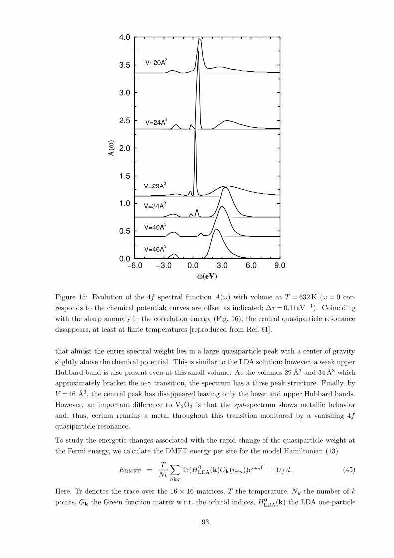
−6.0 −3.0 0.0 3.0 6.0 9.0ω(eV)
0.0
0.5
1.0
1.5
2.0
2.5
3.0
3.5
4.0
Α(ω
)
V=29A3
V=46A3
V=20A3
V=34A3
V=24A3
V=40A3
Figure 15: Evolution of the 4f spectral function A(ω) with volume at T = 632 K (ω = 0 cor-
responds to the chemical potential; curves are offset as indicated; ∆τ = 0.11eV−1). Coinciding
with the sharp anomaly in the correlation energy (Fig. 16), the central quasiparticle resonance
disappears, at least at finite temperatures [reproduced from Ref. 61].
that almost the entire spectral weight lies in a large quasiparticle peak with a center of gravity
slightly above the chemical potential. This is similar to the LDA solution; however, a weak upper
Hubbard band is also present even at this small volume. At the volumes 29 A3 and 34 A3 which
approximately bracket the α-γ transition, the spectrum has a three peak structure. Finally, by
V =46 A3, the central peak has disappeared leaving only the lower and upper Hubbard bands.
However, an important difference to V2O3 is that the spd-spectrum shows metallic behavior
and, thus, cerium remains a metal throughout this transition monitored by a vanishing 4f
quasiparticle resonance.
To study the energetic changes associated with the rapid change of the quasiparticle weight at
the Fermi energy, we calculate the DMFT energy per site for the model Hamiltonian (13)
EDMFT =T
Nk
∑
nkσ
Tr(H0LDA(k)Gk(iωn))eiωn0+
+ Uf d. (45)
Here, Tr denotes the trace over the 16 × 16 matrices, T the temperature, Nk the number of k
points, Gk the Green function matrix w.r.t. the orbital indices, H 0LDA(k) the LDA one-particle
93

−2
−1
0
E−E
PM
HF
(eV
)
T=0.054 eVT=0.136 eVT=0.544 eV
10 20 30 40 50V (Å3)
1.2
1.6
2.0
Eto
t (e
V)
(a)
(b)
α γ
polarized HF
Figure 16: (a) Correlation energy EDMFT−EPMHF as a function of atomic volume (symbols)
and polarized HF energy EAFHF−EPMHF (dotted lines which, at large V, approach the DMFT
curves for the respective temperatures); arrows: observed volume collapse from the α- to the
γ-phase. The correlation energy sharply bends away from the polarized HF energy in the region
of the transition. (b) The resultant negative curvature leads to a growing depression of the total
energy near V =26–28 A3 as temperature is decreased, consistent with an emerging double well
at still lower temperatures and thus the α-γ transition. The curves at T = 0.544 eV were shifted
downwards in (b) by −0.5 eV to match the energy range [reproduced from Ref. 60].
matrix Eq. (15), and
d =1
2
∑′mσ,m′σ′
〈nifmσ nifm′σ′〉 (46)
is a generalization of the one-band double occupation for multi-band models.
Fig. 16a shows our calculated DMFT(QMC) energies EDMFT as a function of atomic volume
at three temperatures relative to the paramagnetic Hartree Fock (HF) energies EPMHF [of the
Hamiltonian (13)], i.e., the energy contribution due to electronic correlations. We also present
the polarized HF energies which basically represent a (non-self-consistent) LDA+U calculation
and reproduceEDMFT at large volumes and low temperatures. With decreasing volume, however,
the DMFT energies bend away from the polarized HF solutions. Thus, at T =0.054 eV≈ 600 K,
a region of negative curvature in EDMFT−EPMHF is evident within the observed two phase region
(arrows).
Fig. 16b presents the calculated LDA+DMFT total energy Etot(T ) =ELDA(T )+EDMFT(T )−EmLDA(T ) where EmLDA is the energy of an LDA-like solution of the Hamiltonian (13).107
Since both ELDA and EPMHF−EmLDA have positive curvature throughout the volume range
considered, it is the negative curvature of the correlation energy in Fig. 16a which leads to the
dramatic depression of the LDA+DMFT total energies in the range V = 26-28 A3 for decreasing
94
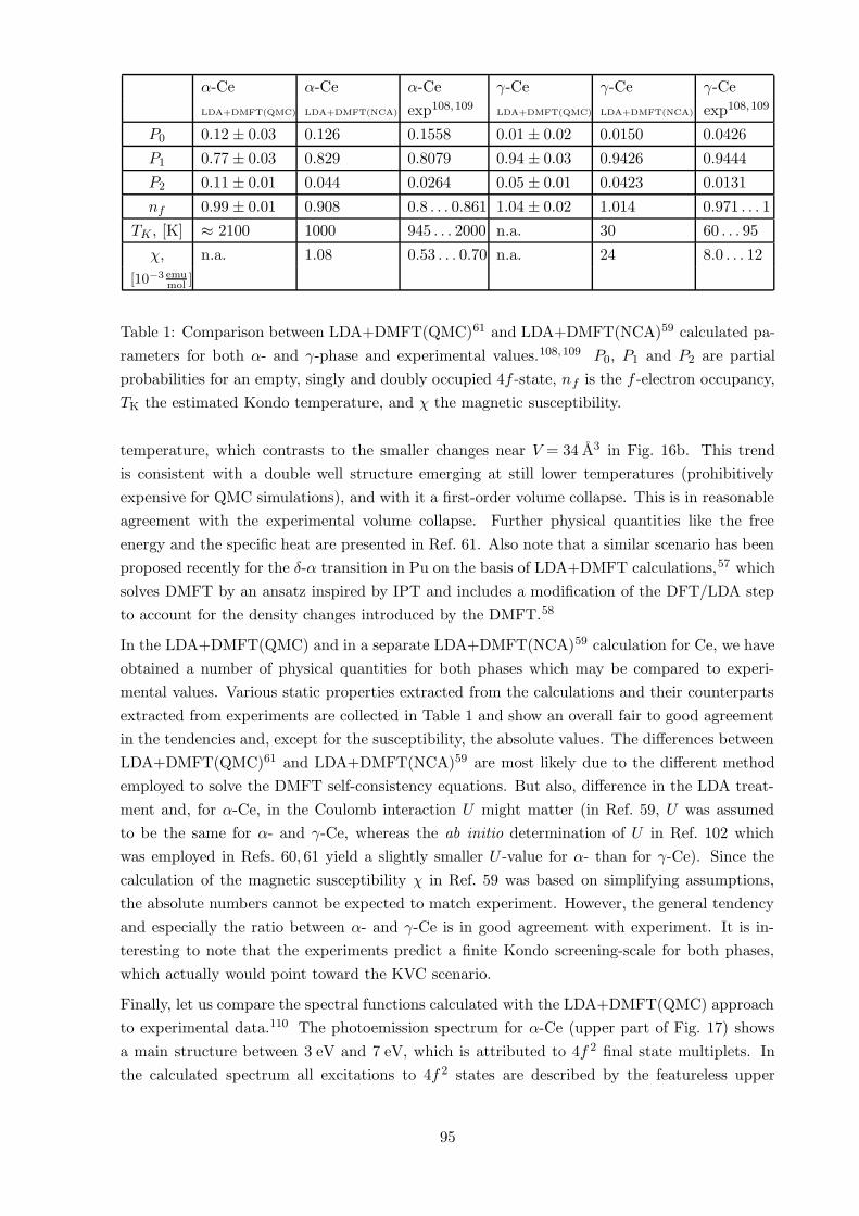
α-Ce α-Ce α-Ce γ-Ce γ-Ce γ-Ce
LDA+DMFT(QMC) LDA+DMFT(NCA) exp108,109LDA+DMFT(QMC) LDA+DMFT(NCA) exp108,109
P0 0.12 ± 0.03 0.126 0.1558 0.01 ± 0.02 0.0150 0.0426
P1 0.77 ± 0.03 0.829 0.8079 0.94 ± 0.03 0.9426 0.9444
P2 0.11 ± 0.01 0.044 0.0264 0.05 ± 0.01 0.0423 0.0131
nf 0.99 ± 0.01 0.908 0.8 . . . 0.861 1.04 ± 0.02 1.014 0.971 . . . 1
TK , [K] ≈ 2100 1000 945 . . . 2000 n.a. 30 60 . . . 95
χ, n.a. 1.08 0.53 . . . 0.70 n.a. 24 8.0 . . . 12
[10−3 emumol ]
Table 1: Comparison between LDA+DMFT(QMC)61 and LDA+DMFT(NCA)59 calculated pa-
rameters for both α- and γ-phase and experimental values.108,109 P0, P1 and P2 are partial
probabilities for an empty, singly and doubly occupied 4f -state, nf is the f -electron occupancy,
TK the estimated Kondo temperature, and χ the magnetic susceptibility.
temperature, which contrasts to the smaller changes near V = 34 A3 in Fig. 16b. This trend
is consistent with a double well structure emerging at still lower temperatures (prohibitively
expensive for QMC simulations), and with it a first-order volume collapse. This is in reasonable
agreement with the experimental volume collapse. Further physical quantities like the free
energy and the specific heat are presented in Ref. 61. Also note that a similar scenario has been
proposed recently for the δ-α transition in Pu on the basis of LDA+DMFT calculations,57 which
solves DMFT by an ansatz inspired by IPT and includes a modification of the DFT/LDA step
to account for the density changes introduced by the DMFT.58
In the LDA+DMFT(QMC) and in a separate LDA+DMFT(NCA)59 calculation for Ce, we have
obtained a number of physical quantities for both phases which may be compared to experi-
mental values. Various static properties extracted from the calculations and their counterparts
extracted from experiments are collected in Table 1 and show an overall fair to good agreement
in the tendencies and, except for the susceptibility, the absolute values. The differences between
LDA+DMFT(QMC)61 and LDA+DMFT(NCA)59 are most likely due to the different method
employed to solve the DMFT self-consistency equations. But also, difference in the LDA treat-
ment and, for α-Ce, in the Coulomb interaction U might matter (in Ref. 59, U was assumed
to be the same for α- and γ-Ce, whereas the ab initio determination of U in Ref. 102 which
was employed in Refs. 60, 61 yield a slightly smaller U -value for α- than for γ-Ce). Since the
calculation of the magnetic susceptibility χ in Ref. 59 was based on simplifying assumptions,
the absolute numbers cannot be expected to match experiment. However, the general tendency
and especially the ratio between α- and γ-Ce is in good agreement with experiment. It is in-
teresting to note that the experiments predict a finite Kondo screening-scale for both phases,
which actually would point toward the KVC scenario.
Finally, let us compare the spectral functions calculated with the LDA+DMFT(QMC) approach
to experimental data.110 The photoemission spectrum for α-Ce (upper part of Fig. 17) shows
a main structure between 3 eV and 7 eV, which is attributed to 4f 2 final state multiplets. In
the calculated spectrum all excitations to 4f 2 states are described by the featureless upper
95

−5.0 0.0 5.0 10.0ω(eV)
0.0
1.0
2.0
3.0
4.0
0.0
1.0
2.0
8.0
9.0
Α(ω
)
V=29A3
V=34A3
α−Ce
γ−Ce
Figure 17: Comparison between combined photoemission110 and BIS111 experimental (circles)
and theoretical LDA+DMFT(QMC) total spectra (solid line) for α- (upper part) and γ-Ce
(lower part) at T = 580 K. The experimental and theoretical spectra were normalized and the
theoretical curve was broadened with resolution width of 0.4 eV [reproduced from Ref. 61].
Hubbard band. As a consequence of the simplified interaction model all doubly occupied states
are degenerate. This shortcoming in our calculation is responsible for the sharply peaked main
structure. The neglected exchange interaction would produce a multiplet structure, which would
be closer to the experiment. The calculated f -spectrum shows a sharp quasiparticle or Kondo
resonance slightly above the Fermi energy, which is the result of the formation of a singlet
state between f - and conduction states. We thus suggest that the spectral weight seen in the
experiment is a result of this quasiparticle resonance. In the lower part of Fig. 17, a comparison
between experiment and our calculation for γ-Ce is shown. The most striking difference between
the lower and the upper part of Fig. 17 is the absence of the Kondo resonance in the γ-phase
which is in agreement with our calculations. Nonetheless γ-Ce remains metallic with spectral
weight arising from the spd-electrons at the Fermi energy. Altogether, one can say that the
agreement with the experimental spectrum is very good, and comparable to the LDA accuracy
for much simpler systems.
7 Conclusion and Outlook
At present LDA+DMFT is the only available ab initio computational technique which is able to
treat correlated electronic systems close to a Mott-Hubbard MIT, heavy fermions, and f -electron
materials. The physical properties of such systems are characterized by the correlation-induced
96

generation of small, Kondo-like energy scales which are missing in the LDA and which require
the application of genuine many-body techniques.
In this paper we discussed the set-up of the computational scheme LDA+DMFT which merges
two non-perturbative, complementary investigation techniques for many-particle systems in solid
state physics. LDA+DMFT allows one to perform ab initio calculations of real materials with
strongly correlated electrons. Using the band structure results calculated within local density
approximation (LDA) as input, the missing electronic correlations are introduced by dynamical
mean-field theory (DMFT). On a technical level this requires the solution of an effective self-
consistent, multi-band Anderson impurity problem by some numerical method (e.g. IPT, NCA,
QMC). Comparison of the photoemission spectrum of La1−xSrxTiO3 calculated by LDA+DMFT
using IPT, NCA, and QMC reveal that the choice of the evaluation method is of considerable
importance. Indeed, only with the numerically exact QMC quantitatively reliable results are
obtained. The results of the LDA+DMFT(QMC) approach were found to be in good agreement
with the experimental photoemission spectrum of La0.94Sr0.06TiO3.
We also presented results of a LDA+DMFT(QMC) study48 of the Mott-Hubbard metal-insulator
transition (MIT) in the paramagnetic phase of (doped) V2O3. These results showed a MIT at
a reasonable value of the Coulomb interaction U ≈ 5 eV and are in very good agreement with
the experimentally determined photoemission and X-ray absorption spectra for this system, i.e.,
above and below the Fermi energy. In particular, we find a spin state S = 1 in the paramagnetic
phase, and an orbital admixture of eπg eπg and eπga1g configurations, which both agree with recent
experiments. Thus, LDA+DMFT(QMC) provides a remarkably accurate microscopic theory of
the strongly correlated electrons in the paramagnetic metallic phase of V2O3.
Another material where electronic correlations are considered to be important is cerium. We
reviewed our recent investigations of the Ce α-γ transition, based on LDA+DMFT(QMC)60,61
and LDA+DMFT(NCA)59 calculations. The spectral results and susceptibilities show the same
tendency as seen in the experiment, namely a dramatic reduction in the size of the quasiparticle
peak at the Fermi level when passing from the α- to the γ-phase. While we do not know at
the moment whether the zero-temperature quasiparticle peak will completely disappear at an
even larger volume (i.e., in a rather Mott-like fashion) or simply fade away continuously with
increasing volume (i.e., in a more Kondo-like fashion), an important aspect of our results is
that the rapid reduction in the size of the peak seems to coincide with the appearance of a
negative curvature in the correlation energy and a shallow minimum in the total energy. This
suggest that the electronic correlations responsible for the reduction of the quasiparticle peak
are associated with energetic changes that are strong enough to cause a volume collapse in the
sense of the Kondo volume collapse model,104 or a Mott transition model103 including electronic
correlations.
We also discussed the embedding of LDA+DMFT in a spectral density functional theory, and ex-
tensions like self-consistent LDA+DMFT calculations, LDA+cluster DMFT, and GW+DMFT.
These extensions are still work in progress which have been applied to model systems or, in the
case of self-consistent LDA+DMFT, to Pu where a fast IPT-inspired DMFT solver has been
employed.57,58 A systematic analysis of the effect of these extensions in the context of realistic
calculations is still mandatory and certainly depends on the system at hand. E.g., one would
97

certainly expect the non-local correlations taken into account by cluster DMFT approaches to be
much more important for effectively one- and two-dimensional systems than in three dimensions.
Another important aspect of future investigations is the calculation of other physical quantities.
In the first LDA+DMFT publications, mainly the local spectral function (Green function) was
calculated because it arises naturally in the DMFT self-consistency scheme. Nonetheless, in
the near future more physical quantities will be calculated by LDA+DMFT: thermodynamic
properties like the specific heat or entropy, which have been already calculated for f -electron
systems but not yet for transition metal oxides; transport properties like the electrical, optical,
and thermal conductivity; magnetic, orbital and other susceptibilities; calculations will also be
performed within symmetry broken phases and phase diagrams will be obtained.
Physicists from two strong solid state communities, i.e., the DFT bandstructure and the many-
body community, have finally joined forces to develop and apply LDA+DMFT. The outcome
is a powerful tool for future investigations of electronic properties of real materials with strong
electronic correlations.
Acknowledgments
We are grateful to J. W. Allen, O. K. Andersen, P. W. Anderson, R. Bulla, R. Claessen, U. Eckern,
G. Esirgen, A. Georges, K.-H. Hock, S. Horn, M. Jarrell, J. Keller, H.-D. Kim, D. E. Kondakov, G. Kotliar,
J. Lægsgaard, A. Lichtenstein, D. van der Marel, W. Metzner, T. M. Rice, G. A. Sawatzky, J. Schmalian,
M. Schramme, M. Sigrist, M. Ulmke, and M. Zolfl for helpful discussions. We thank A. Sandvik for
making available his maximum entropy code. The QMC code of Ref. 33 App. D was modified for use for
some of the results of Section 6. This work was supported in part by the Deutsche Forschungsgemeinschaft
through the Emmy-Noether program (KH), Sonderforschungsbereich 484 (DV, GK, VE), Forschergruppe
HO 955/2 (VE), and project Pr 298/5-1 & 2 (TP), the Russian Foundation for Basic Research by RFFI-
01-02-17063 (VA) and RFFI-02-02-06162 (IN), the U.S. Department of Energy by University California
LLNL under contract No. W-7405-Eng-48. (AM), the U.S. National Science Foundation by DMR-9985978
(RS), the Lorentz Center in Leiden and the Kalvi Institute for Theoretical Physics at the University of
California, Santa Barbara, for their hospitality and support, the Leibniz-Rechenzentrum, Munchen, and
the John v. Neumann-Institut for Computing, Julich.
References
[1] P. Hohenberg and W. Kohn, Phys. Rev. B 136, 864 (1964).
[2] W. Kohn and L. J. Sham, Phys. Rev. 140, 4A, A1133 (1965); W. Kohn and L. J. Sham, Phys. Rev.
A - Gen. Phys. 140, 1133 (1965); L. J. Sham and W. Kohn, Phys. Rev. 145 N 2, 561 (1966).
[3] R. O. Jones and O. Gunnarsson, Rev. Mod. Phys. 61, 689 (1989).
[4] T. C. Leung, X. W. Wang, and B. N. Harmon, Phys. Rev. B 37, 384 (1988); J. Zaanen, O. Jepsen,
O. Gunnarsson, A. T. Paxton, and O. K. Andersen, Physica C 153, 1636 (1988); W. E. Pickett,
Rev. Mod. Phys. 61, 433 (1989).
[5] L. F. Mattheiss, J. Phys.: Cond. Matt. 6, 6477 (1994).
98

[6] K. Held, I. A. Nekrasov, G. Keller, V. Eyert, N. Blumer, A. K. McMahan, R. T. Scalettar, Th. Pr-
uschke, V. I. Anisimov, and D. Vollhardt, in Quantum Simulations of Complex Many-Body Systems:
From Theory to Algorithms, J. Grotendorst, D. Marks, and A. Muramatsu (ed.), NIC Series Volume
10, p. 175-209 (2002).
[7] A. I. Lichtenstein, M. I. Katsnelson, and G. Kotliar, to be published in Electron Correlations and
Materials Properties 2, A. Gonis (ed.), Kluwer, New York; G. Kotliar and S. Savrasov, in New
Theoretical Approaches to Strongly Correlated Systems, A. M. Tsvelik (ed.), Kluwer, New York,
2001, p. 259.
[8] M. Born and R. Oppenheimer, Ann. Phys. (Leipzig) 84, 457 (1927).
[9] M. Levy, Proc. Natl. Acad. Sci. (USA), 76, 6062 (1979).
[10] L. Hedin and B. Lundqvist, J. Phys. C: Solid State Phys. 4, 2064 (1971); U. von Barth and L. Hedin,
J. Phys. C: Solid State Phys. 5, 1629 (1972).
[11] D. M. Ceperley and B. J. Alder, Phys. Rev. Lett. 45, 566 (1980).
[12] O. K. Andersen, Phys. Rev. B 12, 3060 (1975); O. Gunnarsson, O. Jepsen, and O. K. Andersen,
Phys. Rev. B 27, 7144 (1983); O. K. Andersen and O. Jepsen, Phys. Rev. Lett. 53, 2571 (1984).
[13] O. K. Andersen, T. Saha-Dasgupta, S. Ezhov, L. Tsetseris, O. Jepsen, R. W. Tank, C. Arcangeli,
and G. Krier, Psi-k Newsletter 45, 86 (2001).
[14] E. Muller-Hartmann, Z. Phys. B 74, 507 (1989); ibid. B 76, 211 (1989).
[15] J. Wahle, N. Blumer, J. Schlipf, K. Held, and D. Vollhardt, Phys. Rev. B 58, 12749 (1998).
[16] O. Gunnarson, O. K. Andersen, O. Jepsen, and J. Zaanen, Phys. Rev. B 39, 1708 (1989).
[17] I. A. Nekrasov, K. Held, N. Blumer, A. I. Poteryaev, V. I. Anisimov, and D. Vollhardt, Euro. Phys.
J. B 18, 55 (2000).
[18] I. Solovyev, N. Hamada, and K. Terakura, Phys. Rev. B 53, 7158 (1996).
[19] V. I. Anisimov, J. Zaanen, and O. K. Andersen, Phys. Rev. B 44, 943 (1991); V. I. Anisimov, F.
Aryasetiawan, and A. I. Lichtenstein, J. Phys. Cond. Matter 9, 767 (1997).
[20] V. I. Anisimov, A. I. Poteryaev, M. A. Korotin, A. O. Anokhin, and G. Kotliar, J. Phys. Cond.
Matter 9, 7359 (1997).
[21] A. I. Lichtenstein and M. I. Katsnelson, Phys. Rev. B 57, 6884 (1998).
[22] V. Drchal, V. Janis, and J. Kudrnovsky, in Electron Correlations and Material Properties, edited by
A. Gonis, N. Kioussis, and M. Ciftan, Kluwer/Plenum, New York, 1999, p. 273.
[23] J. Lægsgaard and A. Svane, Phys. Rev. B 58, 12817 (1998).
[24] Th. Wolenski, Combining bandstructure and dynamical mean-field theory: A new perspective on
V2O3, Ph.D. Thesis, Universitat Hamburg 1998 (Shaker Verlag, Aachen, 1999).
[25] M. B. Zolfl, Th. Pruschke, J. Keller, A. I. Poteryaev, I. A. Nekrasov, and V. I. Anisimov, Phys. Rev.
B 61, 12810 (2000).
[26] W. Metzner and D. Vollhardt, Phys. Rev. Lett. 62, 324 (1989).
[27] U. Brandt and C. Mielsch, Z. Phys. B 75, 365 (1989); ibid. B 79, 295 (1989); ibid. B 82, 37 (1991).
[28] V. Janis, Z. Phys. B 83, 227 (1991); V. Janis and D. Vollhardt, Int. J. Mod. Phys. 6, 731 (1992).
[29] A. Georges and G. Kotliar, Phys. Rev. B 45, 6479 (1992).
[30] M. Jarrell, Phys. Rev. Lett. 69, 168 (1992).
99

[31] D. Vollhardt, in Correlated Electron Systems, edited by V. J. Emery, World Scientific, Singapore,
1993, p. 57.
[32] Th. Pruschke, M. Jarrell, and J. K. Freericks, Adv. in Phys. 44, 187 (1995).
[33] A. Georges, G. Kotliar, W. Krauth, and M. J. Rozenberg, Rev. Mod. Phys. 68, 13 (1996).
[34] P. W. Anderson, in Moment formation in solids, edited by W. J. L. Buyers, Plenum Press, New
York and London, 1984, p. 313.
[35] W. Negele and H. Orland, Quantum Many-Particle Systems, Addison-Wesley, New York, 1987.
[36] H. Keiter and J. C. Kimball, Phys. Rev. Lett. 25, 672 (1970); N. E. Bickers, D. L. Cox, and J. W.
Wilkins, Phys. Rev. B 36, 2036 (1987).
[37] Th. Pruschke and N. Grewe, Z. Phys. B 74, 439 (1989).
[38] Th. Pruschke, D. L. Cox, and M. Jarrell, Phys. Rev. B 47, 3553 (1993).
[39] J. E. Hirsch and R. M. Fye, Phys. Rev. Lett. 56, 2521 (1986); M. Jarrell, Phys. Rev. Lett. 69, 168
(1992); M. Rozenberg, X. Y. Zhang, and G. Kotliar, Phys. Rev. Lett. 69, 1236 (1992); A. Georges
and W. Krauth, Phys. Rev. Lett. 69, 1240 (1992); M. Jarrell, in Numerical Methods for Lattice
Quantum Many-Body Problems, edited by D. Scalapino, Addison Wesley, 1997.
[40] M. J. Rozenberg, Phys. Rev. B 55, R4855 (1997).
[41] J. E. Han, M. Jarrell, and D. L. Cox, Phys. Rev. B 58, R4199 (1998).
[42] K. Held and D. Vollhardt, Euro. Phys. J. B 5, 473 (1998).
[43] M. Caffarel and W. Krauth, Phys. Rev. Lett. 72, 1545 (1994).
[44] R. Bulla, Adv. Sol. State Phys. 46, 169 (2000).
[45] H. Kajueter and G. Kotliar, Int. J. Mod. Phys. 11, 729 (1997).
[46] M. I. Katsnelson and A. I. Lichtenstein, J. Phys. Cond. Matter 11, 1037 (1999).
[47] M. I. Katsnelson and A. I. Lichtenstein, Phys. Rev. B 61, 8906 (2000).
[48] K. Held, G. Keller, V. Eyert, V. I. Anisimov, and D. Vollhardt, Phys. Rev. Lett. 86, 5345 (2001).
[49] M. S. Laad, L. Craco, and E. Muller-Hartmann, cond-mat/0211210.
[50] I.A. Nekrasov, G. Keller, D.E. Kondakov, A.V. Kozhevnikov, Th. Pruschke, K. Held, D. Vollhardt,
and V.I. Anisimov, cond-mat/0211508; A. Liebsch, cond-mat/0301537.
[51] I.A. Nekrasov, Z.V. Pchelkina, G. Keller, Th. Pruschke, K. Held, A. Krimmel, D. Vollhardt, and
V.I. Anisimov, Phys. Rev. B 67, 85111 (2003).
[52] A. Liebsch and A. I. Lichtenstein, Phys. Rev. Lett. 84, 1591 (2000); A. Liebsch, cond-mat/0301536.
[53] V. I. Anisimov, I. A. Nekrasov, D. E. Kondakov, T. M. Rice, and M. Sigrist, Eur. Phys. J. B 25,
191-201 (2002).
[54] L. Craco, M. S. Laad, and E. Muller-Hartmann, cond-mat/0209132.
[55] A. I. Lichtenstein, M. I. Katsnelson, and G. Kotliar Phys. Rev. Lett. 87, 67205 (2001).
[56] S. Biermann, A. Dallmeyer, C. Carbone, W. Eberhardt, C. Pampuch, O. Rader, M. I. Katsnelson,
and A. I. Lichtenstein, cond-mat/0112430.
[57] S. Y. Savrasov, G. Kotliar, and E. Abrahams, Nature 410, 793 (2001).
[58] S. Y. Savrasov and G. Kotliar, cond-mat/0106308.
100

[59] M. B. Zolfl, I. A. Nekrasov, Th. Pruschke, V. I. Anisimov, and J. Keller, Phys. Rev. Lett. 87, 276403
(2001).
[60] K. Held, A. K. McMahan, and R. T. Scalettar, Phys. Rev. Lett. 87, 276404 (2001).
[61] A. K. McMahan, K. Held, and R. T. Scalettar, Phys. Rev. B 67, 75108 (2003).
[62] W. Weber, J. Bunemann, and F. Gebhard, in Band-Ferromagnetism, edited by K. Baberschke,
M. Donath, and W. Nolting, Lecture Notes in Physics, Vol. 580 (Springer, Berlin, 2001), p. 9; J.
Bunemann, F. Gebhard, W. Weber, Phys. Rev. B 57, 6896 (1998).
[63] M. Suzuki, Prog. Theor. Phys. 56, 1454 (1976)
[64] One limitation of QMC is that it is very difficult to deal with the spin-flip term of the Hund’s
rule coupling because of a “minus-sign problem” which arises in a Hubbard-Stratonovich decoupling
of this spin-flip term, see K. Held, Untersuchung korrelierter Elektronensysteme im Rahmen der
Dynamischen Molekularfeldtheorie, Ph.D. thesis, Universitat Augsburg 1999 (Shaker Verlag, Aachen,
1999). In the particle-hole symmetric case another decoupling scheme which includes the spin-flip
term is possible without “minus-sign problem”, see Y. Motome and M. Imada, J. Phys. Soc. Jap.
66, 1872 (1997).
[65] N. Metropolis, A. W. Rosenbluth, M. N. Rosenbluth, A. H. Teller, and E. Teller, J. Chem. Phys.
21, 1087 (1953).
[66] M. Jarrell and J. E. Gubernatis, Physics Reports 269, 133 (1996).
[67] E. Muller-Hartmann, Z. Phys. B 57, 281 (1984).
[68] G. Kotliar, Physica B 259-261, 711 (1999). R. Chitra and G. Kotliar, Phys. Rev. B 62, 12715 (2000).
[69] R. Fukuda, T. Kotani, and S. Yokojima, Prog. Theory Phys. 92, 833 (1994); R. Fukuda et al., Prog.
Theory Phys. Suppl. 121, 1 (1996).
[70] G. Kotliar, S. Y. Savrasov, G. Palsson, and G. Biroli, Phys. Rev. Lett. 87, 186401 (2001); G. Biroli
and G. Kotliar, Phys. Rev. B 65, 155112 (2002).
[71] A. I. Lichtenstein and M. I. Katsnelson, Phys. Rev. B 62, 9283 (2000).
[72] M. Potthoff, M. Aichhorn, and C. Dahnken, preprint.
[73] M. H. Hettler, A. N. Tahvildar-Zadeh, and M. Jarrell, Phys. Rev. B 58, 7475 (1998); M. H. Hettler,
M. Mukherjee, M. Jarrell, and H. R. Krishnamurthy, Phys. Rev. B 61, 12739 (2000). Note, that one
of the implementations in Ref. 71 is equivalent to DCA.
[74] A. Schiller and K. Ingersent, Phys. Rev. Lett. 75, 113 (1995); G. Zarand, D. L. Cox, and A. Schiller,
Phys. Rev. B 62, 16227 (2000).
[75] Th. Maier, M. Jarrell, Th. Pruschke, and J. Keller, Phys. Rev. Lett. 85, 1524 (2000); Eur. Phys. J.
B 13 613 (2000); C. Huscroft, M. Jarrell, Th. Maier, S. Moukouri, and A. N. Tahvildarzadeh, Phys.
Rev. Lett. 86, 139 (2001).
[76] L. Hedin, Phys. Rev. 139, A796 (1965); F. Aryasetiawan and O. Gunnarsson, Rep. Prog. Phys. 61,
237 (1998).
[77] P. Sun and G. Kotliar, Phys. Rev. B 66, 85120 (2002); S. Biermann, F. Aryasetiawan, and A.
Georges, cond-mat/0207419.
[78] D. A. MacLean, H.-N. Ng, and J. E. Greedan, J. Solid State Chem. 30, 35 (1979).
[79] M. Eitel and J. E. Greedan, Journal of the Less-Common Metals 116, 95 (1986).
[80] J. P. Gopel, J. E. Greedan, and D. A. MacLean, J. Solid State Chem. 43, 244 (1981).
101

[81] Y. Okimoto, T. Katsufuji, Y. Okada, T. Arima, and Y. Tokura, Phys. Rev. B 51, 9581 (1995).
[82] W. Heindl, Th. Pruschke, and J. Keller, J. Phys. – Condens. Matter 12, 2245 (2000).
[83] At present, QMC simulations of the DMFT equations are not feasible at the experimental tem-
perature (80K). We note, however, that no intrinsic temperature dependence was observed in the
experiment,84 at least up to room temperature.
[84] A. Fujimori et al, Phys. Rev. Lett. 69, 1796 (1992). A. Fujimori et al, Phys. Rev. B 46, 9841 (1992).
A qualitatively and quantitatively similar spectrum was obtained recently by T. Yoshida, A. Ino, T.
Mizokawa, A. Fujimori, Y. Taguchi, T. Katsufuji, and Y. Tokura, Europhys. Lett. 59, 258 (2002),
with an experimental energy resolution of only 30 meV. One may suppose, however, that broadening
effects due to the polycrystalline nature of the sample and surface effects are, then, larger than the
instrumental resolution.
[85] B. Keimer, D. Casa, A. Ivanov, J.W. Lynn, M. v. Zimmermann, J.P. Hill, D. Gibbs, Y. Taguchi,
and Y. Tokura, Phys. Rev. Lett. 85, 3946 (2000).
[86] N. F. Mott, Rev. Mod. Phys. 40, 677 (1968); Metal-Insulator Transitions (Taylor & Francis, London,
1990); F. Gebhard, The Mott Metal-Insulator Transition (Springer, Berlin, 1997).
[87] D. B. McWhan et al., Phys. Rev. B 7, 1920 (1973).
[88] J. Hubbard, Proc. Roy. Soc. London Ser. A 276, 238 (1963); 277, 237 (1963); 281, 401 (1964).
[89] W. F. Brinkman and T. M. Rice, Phys. Rev. B 2, 4302 (1970).
[90] G. Moeller, Q. Si, G. Kotliar, and M. Rozenberg, Phys. Rev. Lett. 74, 2082 (1995); J. Schlipf, M.
Jarrell, P. G. J. van Dongen, N. Blumer, S. Kehrein, Th. Pruschke, and D. Vollhardt, Phys. Rev.
Lett. 82, 4890 (1999); M. J. Rozenberg, R. Chitra, and G. Kotliar, Phys. Rev. Lett. 83, 3498 (1999);
R. Bulla, Phys. Rev. Lett. 83, 136 (1999); R. Bulla, T. A. Costi, and D. Vollhardt, Phys. Rev. B 64,
45103 (2001); J. Joo and V. Oudovenko, Phys. Rev. B 64, 193102 (2001); N. Blumer, Mott-Hubbard
Metal-Insulator Transition and Optical Conductivity in High Dimensions, Ph.D. thesis, Universitat
Augsburg 2002.
[91] P. D. Dernier, J. Phys. Chem. Solids 31, 2569 (1970).
[92] Use of the crystal structure of Cr-doped V2O3 for the insulating phase of pure V2O3 is justified by
the observation that Cr-doping is equivalent to the application of (negative) pressure.
[93] M. Schramme, Ph.D. thesis, Universitat Augsburg 2000 (Shaker Verlag, Aachen, 2000);
M. Schramme et al. (unpublished).
[94] S.-K. Mo, J. D. Denlinger, H.-D. Kim, J.-H. Park, J. W. Allen, A. Sekiyama, A. Yamasaki,
K. Kadono, S. Suga, Y. Saitoh, T. Muro, P. Metcalf, G. Keller, K. Held, V. Eyert, V. I. Anisi-
mov, and D. Vollhardt, cond-mat/0212110.
[95] O. Muller, J. P. Urbach, E. Goering, T. Weber, R. Barth, H. Schuler, M. Klemm, S. Horn, and M.
L. denBoer, Phys. Rev. B 56, 15056 (1997).
[96] J.-H. Park, L. H. Tjeng, A. Tanaka, J. W. Allen, C. T. Chen, P. Metcalf, J. M. Honig, F. M. F. de
Groot, and G. A. Sawatzky, Phys. Rev. B 61, 11 506 (2000).
[97] D. J. Arnold and R. W. Mires, J. Chem. Phys. 48, 2231 (1968).
[98] C. Castellani, C. R. Natoli, and J. Ranninger, Phys. Rev. B 18, 4945 (1978); 18, 4967 (1978); 18,
5001 (1978).
[99] M. J. Rozenberg, G. Kotliar, H. Kajueter, G. A. Thomas, D. H. Rapkine, J. M. Honig, and P.
Metcalf, Phys. Rev. Lett. 75, 105 (1995).
102

[100] Handbook on the Physics and Chemistry of Rare Earths, edited by K. A. Gschneider Jr. and L. R.
Eyring (North-Holland, Amsterdam, 1978); in particular, D. G. Koskenmaki and K. A. Gschneider
Jr., ibid, p.337.
[101] J. S. Olsen, L. Gerward, U. Benedict, and J.-P. Itie, Physica 133B, 129 (1985).
[102] A. K. McMahan, C. Huscroft, R. T. Scalettar, and E. L. Pollock, J. Comput.-Aided Mater. Design
5, 131 (1998).
[103] B. Johansson, Philos. Mag. 30, 469 (1974); B. Johansson, I.A. Abrikosov, M. Alden, A. V. Ruban,
and H.L. Skriver Phys. Rev. Lett. 74, 2335 (1995).
[104] J. W. Allen and R. M. Martin, Phys. Rev. Lett. 49, 1106, (1982); J. W. Allen and L. Z. Liu, Phys.
Rev. B 46, 5047, (1992); M. Lavagna, C. Lacroix, and M. Cyrot, Phys. Lett. 90A, 210 (1982).
[105] K. Held, C. Huscroft, R.T. Scalettar, and A.K. McMahan, Phys. Rev. Lett. 85, 373 (2000); see
also C. Huscroft, A. K. McMahan, and R. T. Scalettar, Phys. Rev. Lett. 82, 2342 (1999).
[106] K. Held and R. Bulla, Eur. Phys. J. B 17, 7 (2000).
[107] We solve self-consistently for nf using a 4f self energy Σ = Uf (nf − 12 ), and then remove this
contribution from the eigenvalue sum to get the kinetic energy. The potential energy is taken to be12Ufnf (nf − 1).
[108] L. Z. Liu, J. W. Allen, O. Gunnarsson, N. E. Christensen, and O. K. Andersen, Phys. Rev. B 45,
8934 (1992).
[109] A. P. Murani, Z. A. Bowden, A. D. Taylor, R. Osborn, and W. G. Marshall, Phys. Rev B 48, 13981
(1993).
[110] D. M. Wieliczka, C. G. Olson, and D. W. Lynch, Phys. Rev. B 29, 3028 (1984).
[111] E. Wuilloud, H. R. Moser, W. D. Schneider, and Y. Baer, Phys. Rev. B 28, 7354 (1983).
103
![Example: MnO LDA+DMFT in COMSUITE · • 'proj_win_max': High-energy cutoff to renormalize the projectors. The default value is the one specified in wan_hmat[‘dis_win_max’] In](https://static.fdocuments.us/doc/165x107/5f210f7b91e61a479c69005c/example-mno-ldadmft-in-comsuite-a-projwinmax-high-energy-cutoff-to-renormalize.jpg)


![Generalized Correspondence-LDA Models (GC-LDA) for ... · The GC-LDA and Correspondence-LDA models are extensions of Latent Dirichlet Allocation (LDA) [3]. Several Bayesian methods](https://static.fdocuments.us/doc/165x107/6011a7de37d63b741248406f/generalized-correspondence-lda-models-gc-lda-for-the-gc-lda-and-correspondence-lda.jpg)