www.nasa.gov

Lattice Boltzmann Method for Spacecraft Propellant Slosh

Simulation Jeb S. Orr, PhD

The Charles Stark Draper Laboratory, Inc. Jacobs ESSSA Group

Joseph F. Powers

NASA Marshall Space Flight Center Control Systems Design and Analysis Branch (EV41)

H. Q. Yang, PhD

CFD Research Corporation Jacobs ESSSA Group

2015 American Astronautical Society (AAS) Guidance, Navigation, and Control Conference

Breckenridge, CO Jan 30-Feb 4, 2015

https://ntrs.nasa.gov/search.jsp?R=20150006883 2018-06-05T12:19:48+00:00Z

♦  Microgravity propellant dynamics continue to offer a formidable modeling challenge for the computational fluid mechanics community

• Analytical approaches to prediction of bulk behavior, e.g. tank forces and moments, degrades in accuracy below Bo~10; small perturbations only

• Flows dominated by surface tension; curved interfaces; fluid-wall contact angles approximately zero

• Many semi-analytical or empirical methods that correlate well with theory rely on quasi-steady-state parameters and cannot accurately predict effects of transient flows, e.g. throttling, thruster pulses

• Momentum transfer due to fluid must be computed accurately for simulation-based verification

♦  Our research explores the applicability of the lattice Boltzmann method (LBM) to modeling of cryogenic propellant dynamics in microgravity

Introduction

2

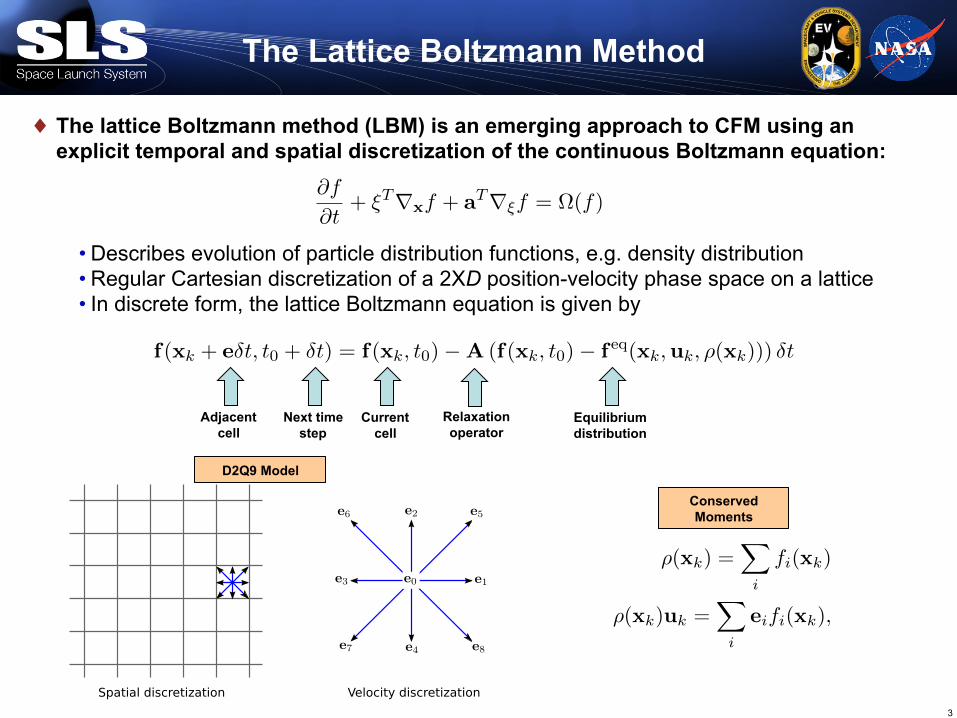
♦  The lattice Boltzmann method (LBM) is an emerging approach to CFM using an explicit temporal and spatial discretization of the continuous Boltzmann equation:

• Describes evolution of particle distribution functions, e.g. density distribution • Regular Cartesian discretization of a 2XD position-velocity phase space on a lattice • In discrete form, the lattice Boltzmann equation is given by

The Lattice Boltzmann Method

3

typically restricted to very low-velocity flows, it does provide several unique advantages over tradi-tional solvers. First, the meshing of complex geometry is performed on a regular cartesian lattice offluid cells, each having uniform volume in the fluid domain. As such, computations involving fluxacross the boundary of adjacent cells are considerably simplified. Secondly, LBE has the advantageof data locality; LBE-based flow solvers are not required to solve a global continuity equation ateach time step. Finally, LBE is relatively simple to implement and computationally efficient.

In the following sections, the development of an LBE-based flow solver for spacecraft propellantdynamics will be detailed. In Section 2, the theory and basic implementation details of the LBEwill be introduced. In Section 3, the method of introducing multi-phase behavior into the LBE willbe discussed. In Section 4, the results of test cases that compare the outputs of the LBE flow solverwith theoretical predictions will be presented. In Section 5, a summary of the present research willbe provided along with some opportunities for forward work.

2 THE LATTICE BOLTZMANN METHOD

The lattice Boltzmann equation (LBE) is a discretization of the continuous Boltzmann equation,describing particle dynamics on a molecular scale. The Boltzmann equation is given by

@f

@t

+ ⇠

Trx

f + a

Tr⇠

f = ⌦(f) (1)

where f(x, ⇠, t) is the molecular velocity distribution function (DF) in the phase space (x, ⇠) wherex 2 RD is the spatial position and ⇠ 2 RD is the velocity. The derivation of the Boltzmannequation follows from the statistical kinetic theory of dilute gases in a closed domain. Here, a is theacceleration due to the applied body force at the spatial location x, and the collision integral is givenby ⌦. The right-hand side of the Boltzmann equation is the collision term describing the short-rangemolecular interactions of the velocity distributions assuming the modeled fluid is a dilute gas.

The direct computation of the collision operator is, in general, intractable for the continuousBoltzmann equation. However, it can be approximated by a relaxation operation that preserves thehydrodynamic moments that are invariants of the collision. In the simplest models, such as the BGK(Bhatnagar-Gross-Krook) approximation, the collision is approximated by a linear relaxation to theequilibrium distribution, which is related to the temperature and velocity of the flow.

The lattice Boltzmann equation follows from discretization of the 2D-dimensional phase spaceand the local approximation of the resultant linear system of ordinary differential equations in dis-crete time, and the approximation of the equilibrium distribution function consistent with that ve-locity discretization. For the present model D = 2 and a velocity discretization of 9 directions intwo dimensions is chosen. The spatial discretization is applied on a regular lattice of size �x with atemporal discretization �t. The lattice structure shown in Figure 1 is known as the D2Q9 model.

The lattice parameter c = �x/�t defines the characteristic speed associated with the velocity dis-cretization e

i

, i = 0, 1, . . . 8. In this discretization, the k

th cell at spatial location x

k

is describedby a distribution function f(x

k

, t) 2 R9, the velocity distribution function at the lattice site xk

. Thei

th component of the discretized distribution function describes the density of particles at xk

havingvelocity e

i

. The approximation of the equilibrium distribution f

eq (namely, the Maxwell equilib-rium) is carried out such that the kinetic hydrodynamic moments are consistently approximated afterdiscretization. The continuous Maxwell distribution is expanded to third order in the velocity; thetruncated equilibrium approximation then converted into a discretized form using a Gauss-Hermite

2

Figure 1. D2Q9 Lattice Structure

quadrature. The solution of the discretized Boltzmann equation can then be approximated by

f(xk

+ e�t, t0 + �t) = f(xk

, t0)�A (f(xk

, t0)� f

eq(xk

,u

k

, ⇢(xk

))) �t. (2)

where u

k

is the local velocity, and the collision matrix A has been introduced. The conservedhydrodynamic moments are given by

⇢(xk

) =X

i

f

i

(xk

) (3)

⇢(xk

)uk

=X

i

e

i

f

i

(xk

), (4)

and the speed of sound is cs

= c/

p3.

Equation (2) is the lattice Boltzmann equation. Under certain conditions, it is possible to recoverthe macroscopic transport and continuity equations using the Chapman-Enskog expansion of theLBE.3 The approximation of incompressible flow is valid only at small velocities for steady flow,owing partially to the velocity truncation. This implies that compressibility error is the dominanterror source in the application of LBE.

The LBE is typically implemented in two steps comprising advection (streaming) and collision(relaxation) using two copies of the domain, f and f

0. The boundary conditions are applied at latticesites where fluid cells are adjacent to a specified boundary, such as a wall. In almost all numericalimplementations, the units associated with the lattice are chosen such that �x = �t = c = 1 andthe mean density ⇢̄ is on the order of 1. This greatly reduces the computational burden and providesgood numerical conditioning for the requisite computations.

In the following developments, the spatial dependency of the hydrodynamic quantities will bedenoted with a subscript k for brevity, and the temporal dependency is implied.

2.1 Relaxation Operation

In implementations of the LBE using the BGK approximation, the collision matrix is replacedby a scalar relaxation frequency ! = 1

⌧

where ⌧ is the relaxation time. In this single relaxationtime (SRT) model, all populations relax toward equilibrium at the same rate. It has been recognizedthat while the SRT model is simple to implement, the relaxation of all populations at the same

3

Adjacent cell

Next time step

Current cell

Equilibrium distribution

Relaxation operator

D2Q9 Model

⇢(xk) =X

i

fi(xk)

⇢(xk)uk =X

i

eifi(xk),

Conserved Moments

♦  The fluid dynamics are propagated in two steps over multiple layers

1.  Advection (copy fluid density to adjacent cell: “streaming”)

2.  Collision (simulate collisions by relaxing toward Maxwell equilibrium: “relaxation”)

♦  Proper choice of units (time=space=1) and periodic lattice: no actual data copy •  The streaming step is done using pointer

arithmetic: fast •  Data locality (only need knowledge of

adjacent cells): parallelization

♦  Limitations: •  Constant (wall) temperature: isothermal flow •  Effective speed of sound is related to the

lattice physical parameters –  Compressibility error increases as M>0.1 –  Incompressible flow approximation is valid

only for steady flow at low velocities •  Stability decreases as timestep decreases at

a fixed kinematic viscosity

Numerical Implementation and Limitations

4

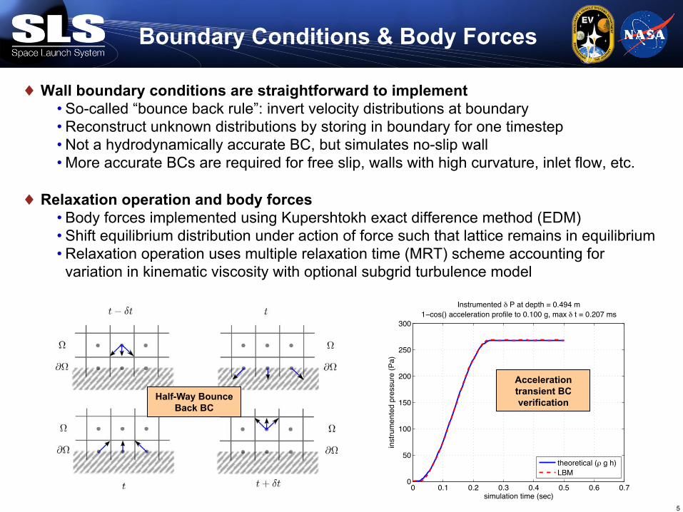
♦  Wall boundary conditions are straightforward to implement • So-called “bounce back rule”: invert velocity distributions at boundary • Reconstruct unknown distributions by storing in boundary for one timestep • Not a hydrodynamically accurate BC, but simulates no-slip wall • More accurate BCs are required for free slip, walls with high curvature, inlet flow, etc.

♦  Relaxation operation and body forces • Body forces implemented using Kupershtokh exact difference method (EDM) • Shift equilibrium distribution under action of force such that lattice remains in equilibrium • Relaxation operation uses multiple relaxation time (MRT) scheme accounting for

variation in kinematic viscosity with optional subgrid turbulence model

Boundary Conditions & Body Forces

5

Half-Way Bounce Back BC

0 0.1 0.2 0.3 0.4 0.5 0.6 0.70

50

100

150

200

250

300

Instrumented b P at depth = 0.494 m1−cos() acceleration profile to 0.100 g, max b t = 0.207 ms

simulation time (sec)

inst

rum

ente

d pr

essu

re (P

a)

theoretical (l g h)LBM

Acceleration transient BC verification

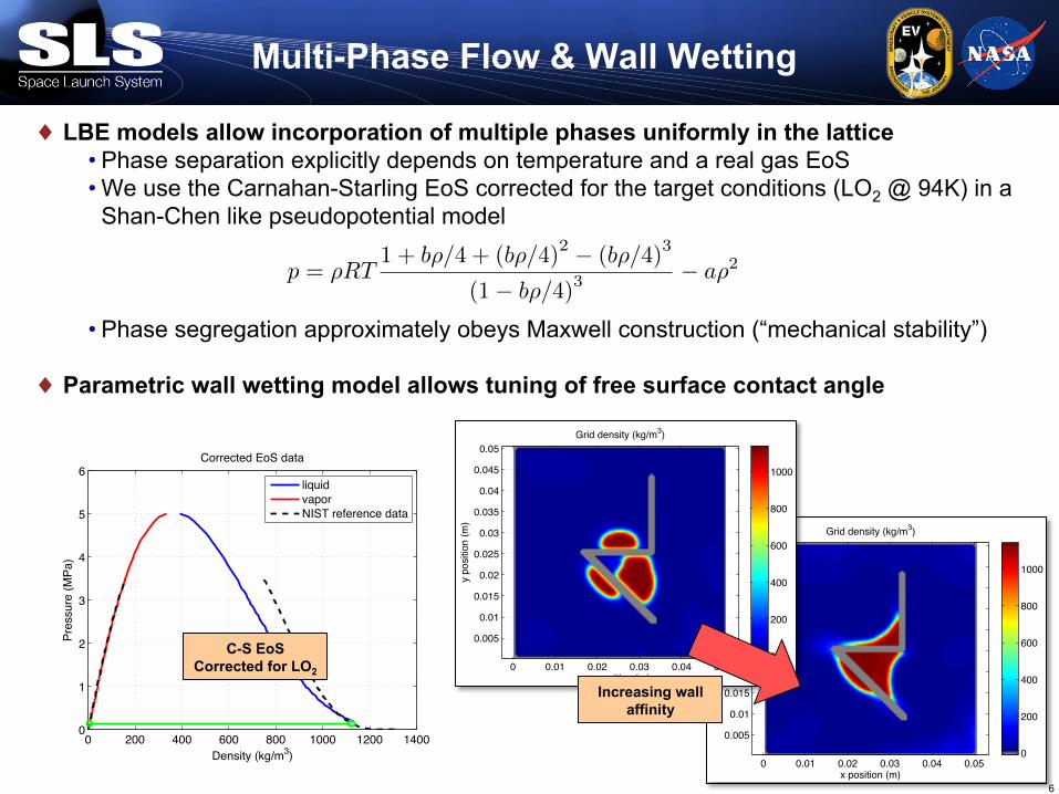
♦  LBE models allow incorporation of multiple phases uniformly in the lattice • Phase separation explicitly depends on temperature and a real gas EoS • We use the Carnahan-Starling EoS corrected for the target conditions (LO2 @ 94K) in a

Shan-Chen like pseudopotential model

• Phase segregation approximately obeys Maxwell construction (“mechanical stability”)

♦  Parametric wall wetting model allows tuning of free surface contact angle

Multi-Phase Flow & Wall Wetting

6

p = ⇢RT1 + b⇢/4 + (b⇢/4)2 � (b⇢/4)3

(1� b⇢/4)3� a⇢2

0 200 400 600 800 1000 1200 14000

1

2

3

4

5

6

Density (kg/m3)

Pres

sure

(MPa

)

Corrected EoS data

liquidvaporNIST reference data

C-S EoS Corrected for LO2

x position (m)

y po

sitio

n (m

)

Grid density (kg/m3)

0 0.01 0.02 0.03 0.04 0.05

0.005

0.01

0.015

0.02

0.025

0.03

0.035

0.04

0.045

0.05

0

200

400

600

800

1000

x position (m)

y po

sitio

n (m

)

Grid density (kg/m3)

0 0.01 0.02 0.03 0.04 0.05

0.005

0.01

0.015

0.02

0.025

0.03

0.035

0.04

0.045

0.05

0

200

400

600

800

1000

Increasing wall affinity

♦  The behavior of droplets in microgravity is dominated by surface tension • Droplet dynamics provide a useful verification case due to analytical solutions • Oscillation of the free surface can be predicted by Lamb’s equation • Effective surface tension can be determined from frequency

Simulating Droplet Dynamics

7

!2 =l(l � 1)(l + 2)

r3⇢L�

Droplet Modes*

*Frohn, A., and Roth, N. Dynamics of Droplets. Springer, 2000

Mode frequency Droplet

radius

Surface tension

0.5 1 1.5 2 2.5 3 3.5 4 4.5 5 5.5

−3

−2

−1

0

1

2

3

4

x 10−3

time (sec)

latti

ce p

ress

ure

[lu]

0.756 secl=2 (~1.3 Hz)

l=6 (~9.3 Hz)

♦  Propellant sloshing dynamics are of fundamental concern in spacecraft dynamics • Analytical solutions exist for axisymmetric containers at high Bo • Below Bo=1000 modified analytical models must be used

– Stable flow only (continuous free surface) and small perturbations • CFD solutions required for turbulent flow, transient phenomena, PMD simulation, etc.

♦  LBE method verified using a flow regime near analytical limit • 0.15 m cylindrical LO2 tank with hemispherical ends @ 0.001 g (Bo=20) • Lattice size = 3462 (4.1 MB) • Free decay from initial condition with acceleration 15 degrees from symmetry axis • First mode frequency matches analytical predictions very well (f=0.055 Hz)

Propellant Slosh (Low Bo)

8

♦  LBM approach used for small domain simulation in microgravity • 0.1m spherical LO2 container in microgravity • High-g initial condition (settled fluid) and 0g at t=0 (20% fill fraction) • Random perturbing acceleration (-3 dB @ 0.2 Hz, gRMS=0.00003) • Lattice size = 2662 (2.4 MB)

Fluid Slosh (Microgravity)

9

t=8s t=20s t=60s t=75s

t=90s T=130s T=150s T=180s

♦  Some promising results have been obtained in the application of the LBE to propellant sloshing dynamics and related microgravity fluid phenomena

• The LBE method has promise for simulation of thermodynamically consistent multiphase flows in cryogenic propellants

• Fundamental stability limitations remain for very low kinematic viscosities (real fluids!) • Recent progress includes stability enhancement via adaptive time-stepping and

improvement in surface tension model using multirange pseudopotential – Overcomes some stability and surface tension limitations by improving isotropy

♦  Production simulation of cryogenic flows will require incorporation of thermal effects • Thermal LBE codes are emerging and show some promise • Important to capture convective phenomena, for example, for modeling of long-term fluid

circulation in propellant storage systems

♦  Ongoing work extends the present proof-of-concept model to a 3D code • Parallelization opportunities may allow simulation of CFD-in-the-loop with spacecraft

GN&C 6-DoF simulations, for example, using GPU computing • Possible validation opportunities using existing microgravity fluid experiment data

collected aboard International Space Station (ISS) • 3D code targeted for NASA Exploration Upper Stage (EUS) ullage settling and propellant

management studies

Forward Work

10