Large-Scale Motion Modelling using a Graphical Processing Unit

Large-Scale Motion Modelling using a Graphical

Processing Unit

LARGE-SCALE MOTION MODELLING USING A GRAPHICAL

PROCESSING UNIT

BY

YUSUF DINATH, B.Eng.

a thesis

submitted to the department of electrical & computer engineering

and the school of graduate studies

of mcmaster university

in partial fulfilment of the requirements

for the degree of

Master of Applied Science

c© Copyright by Yusuf Dinath, August 2012

All Rights Reserved

Master of Applied Science (2012) McMaster University

(Electrical & Computer Engineering) Hamilton, Ontario, Canada

TITLE: Large-Scale Motion Modelling using a Graphical Process-

ing Unit

AUTHOR: Yusuf Dinath

B.Eng., (Electrical Engineering)

McMaster University, Hamilton, Canada

SUPERVISOR: Dr. T. Kirubarajan

NUMBER OF PAGES: xiii, 59

ii

Abstract

The increased availability of Graphical Processing Units (GPUs) in personal comput-

ers has made parallel programming worthwhile and more accessible, but not neces-

sarily easier. This thesis will take advantage of the power of a GPU, in conjunction

with the Central Processing Unit (CPU), in order to simulate target trajectories for

large-scale scenarios, such as wide-area maritime or ground surveillance. The idea is

to simulate the motion of tens of thousands of targets using a GPU by formulating

an optimization problem that maximizes the throughput. To do this, the proposed

algorithm is provided with input data that describes how the targets are expected

to behave, path information (e.g., roadmaps, shipping lanes), and available compu-

tational resources. Then, it is possible to break down the algorithm into parts that

are done in the CPU versus those sent to the GPU. The ultimate goal is to compare

processing times of the algorithm with a GPU in conjunction with a CPU to those of

the standard algorithms running on the CPU alone. In this thesis, the optimization

formulation for utilizing the GPU, simulation results on scenarios with a large number

of targets and conclusions are provided.

iii

Acknowledgements

First and foremost I would like that thank my supervisor, Dr. T. Kiruba, for allowing

me to be his research student during my undergrad studies, a summer student after

completing my undergrad degress and finally his master’s degree student for the past

two years. Also, I would like to thank Dr. R. Tharmarasa for his endless support,

guidance and direction.

I am grateful for the opportunity that Dr. M. McDonald extended during my first

summer as a master’s student, which allowed me to work in Ottawa for the Defence

Research and Development Canada in the Radar Systems group. It provided me with

valuable knowledge and work experience. I also thank Dr. A. Patriciu for sharing his

knowledge and understanding of how to program in parallel using the GPU.

I appreciate and would like to thank Dr. I. Bruce and Dr. A. Jeremic for being

my committee members and for providing feedback on my thesis.

Finally, I would also like to thank Mrs. C. Gies, Graduate Administrative Assis-

tant, who ensures that the ECE department runs smoothly.

iv

Abbreviations

1D One-Dimensional Space

2D Two-Dimensional Space

3D Three-Dimensional Space

BIH Bureau International de l’Heure

CPU Central Processing Unit

CUDA Compute Unified Device Architecture

ECEF Earth-Centered, Earth-Fixed

GFLOPS Giga Floating-Point Operations Per Second

GPU Graphical Processing Unit

GPGPU General Purpose Graphical Processing Unit

ICAO International Civil Aviation Organization

LSMM Large-Scale Motion Models

PC Personal Computer

WGS-84 World Geodetic System - 1984

v

Notation

Γ Total noise added to a state

λ Longitude

ν White noise vector

ω Turn rate

φ Latitude

θ Target’s heading

υλ Ground velocity, longitudial-wise

υφ Ground velocity, latitude-wise

a Semi-major axis

b Semi-minor axis

e First eccentricity

f Ellipsoidal flattening (or oblateness)

F State transition natrix

G Gain matrix

GB/s Gigabytes per second

h Altitude

L Number of targets

k Time step

vi

m Metre

ML Number of motion legs for a target

Mm Number of Monte Carlo runs

Rm Radii of curvature in the meridian

Rv Radii of curvature in the prime vertical

S Speed up factor of two execution times

s Second

T Time difference between k and (k − 1)

t(·) Execution time of a program

xk State at time k

vii

Contents

Abstract iii

Acknowledgements iv

Abbreviations v

Notation vi

1 Introduction and Problem Statement 1

1.1 Related Publication . . . . . . . . . . . . . . . . . . . . . . . . . . . . 5

2 Target Generation 6

2.1 Targets . . . . . . . . . . . . . . . . . . . . . . . . . . . . . . . . . . . 6

2.2 Coordinate Systems . . . . . . . . . . . . . . . . . . . . . . . . . . . . 8

2.2.1 Cartesian Coordinates System . . . . . . . . . . . . . . . . . . 8

2.2.2 WGS-84 . . . . . . . . . . . . . . . . . . . . . . . . . . . . . . 9

2.2.3 ECEF . . . . . . . . . . . . . . . . . . . . . . . . . . . . . . . 12

2.3 Motion Models . . . . . . . . . . . . . . . . . . . . . . . . . . . . . . 12

2.3.1 Non-Maneuvering Targets . . . . . . . . . . . . . . . . . . . . 13

2.3.2 Maneuvering Targets . . . . . . . . . . . . . . . . . . . . . . . 13

viii

2.3.3 3D Models . . . . . . . . . . . . . . . . . . . . . . . . . . . . . 14

2.4 Coordinate Transformation . . . . . . . . . . . . . . . . . . . . . . . . 17

2.4.1 Converting from WGS-84 to ECEF . . . . . . . . . . . . . . . 17

2.4.2 Converting from ECEF to WGS-84 . . . . . . . . . . . . . . . 17

2.5 Process Noise . . . . . . . . . . . . . . . . . . . . . . . . . . . . . . . 18

2.6 Target Generation Theory . . . . . . . . . . . . . . . . . . . . . . . . 18

3 GPU Programming 21

3.1 GPU . . . . . . . . . . . . . . . . . . . . . . . . . . . . . . . . . . . . 21

3.2 CUDA . . . . . . . . . . . . . . . . . . . . . . . . . . . . . . . . . . . 22

3.3 CUDA C Programming . . . . . . . . . . . . . . . . . . . . . . . . . . 23

3.3.1 Memory . . . . . . . . . . . . . . . . . . . . . . . . . . . . . . 23

3.3.2 Toolkit . . . . . . . . . . . . . . . . . . . . . . . . . . . . . . . 24

3.3.3 Libraries . . . . . . . . . . . . . . . . . . . . . . . . . . . . . . 25

3.4 CUDA and the Best Practices . . . . . . . . . . . . . . . . . . . . . . 25

4 CPU and GPU Simulation 27

4.1 Target Trajectories . . . . . . . . . . . . . . . . . . . . . . . . . . . . 27

4.2 Large-Scale Motion Models with Path Unconstrained Targets . . . . . 28

4.3 Large-Scale Motion Models with Constrained Targets . . . . . . . . . 29

4.4 Approach 1: The CPU Algorithm . . . . . . . . . . . . . . . . . . . . 30

4.5 Approach 2: The GPU Algorithm . . . . . . . . . . . . . . . . . . . . 31

4.5.1 Parallel Prefix Sum (Scan) with CUDA . . . . . . . . . . . . . 31

4.5.2 Kernel . . . . . . . . . . . . . . . . . . . . . . . . . . . . . . . 34

4.5.3 Kernel Inputs . . . . . . . . . . . . . . . . . . . . . . . . . . . 39

ix

4.5.4 CUDA Best Practices Implemented in the Kernel . . . . . . . 40

5 Results 41

5.1 Performance Measurements . . . . . . . . . . . . . . . . . . . . . . . 43

5.1.1 Execution Time . . . . . . . . . . . . . . . . . . . . . . . . . . 43

5.1.2 Speedup Factor . . . . . . . . . . . . . . . . . . . . . . . . . . 44

5.1.3 GFLOPS . . . . . . . . . . . . . . . . . . . . . . . . . . . . . 45

5.1.4 Bandwidth . . . . . . . . . . . . . . . . . . . . . . . . . . . . . 45

5.2 Scenario 1 . . . . . . . . . . . . . . . . . . . . . . . . . . . . . . . . . 46

5.3 Scenario 2 . . . . . . . . . . . . . . . . . . . . . . . . . . . . . . . . . 50

5.4 Final Thoughts about Both Simulations . . . . . . . . . . . . . . . . 54

6 Conclusion and Future Work 55

x

List of Figures

2.1 Cartesian coordinate system defined by the right-hand rule . . . . . 9

2.2 WGS-84 Coordinate system definition . . . . . . . . . . . . . . . . . . 11

2.3 Spherical motion of a target from k − 1 to k (Galben, 2011). . . . . . 16

4.1 Sequential pseudocode for the CPU algorithm. . . . . . . . . . . . . . 30

4.2 Motion Leg Parallelization pseudocode for the GPU algorithm. . . . . 31

4.3 Work-efficient parallel scan, up and down sweep (Harris, 2008) . . . . 33

4.4 Vector with 16 elements. . . . . . . . . . . . . . . . . . . . . . . . . . 34

4.5 Scanned vector with 16 elements. . . . . . . . . . . . . . . . . . . . . 35

4.6 Scanned vector with 16 elements. . . . . . . . . . . . . . . . . . . . . 35

4.7 Noise at every time step of a motion leg. . . . . . . . . . . . . . . . . 36

4.8 The scan of Figure 4.7. . . . . . . . . . . . . . . . . . . . . . . . . . . 36

4.9 F-matrix at every time step. . . . . . . . . . . . . . . . . . . . . . . . 37

4.10 The scan of Figure 4.9. . . . . . . . . . . . . . . . . . . . . . . . . . . 37

4.11 Inverse of each element of the scanned F-matrix vector (Figure 4.10). 38

5.1 Sequential pseudocode for the CPU algorithm. . . . . . . . . . . . . . 44

5.2 CPU and GPU execution time versus the duration of the motion leg

for scenario 1. . . . . . . . . . . . . . . . . . . . . . . . . . . . . . . . 47

xi

5.3 Speedup factor of the GPU over the CPU vs the Duration of the Motion

Leg for scenario 1. . . . . . . . . . . . . . . . . . . . . . . . . . . . . 48

5.4 CPU and GPU execution time versus the number of targets for scenario

2. . . . . . . . . . . . . . . . . . . . . . . . . . . . . . . . . . . . . . . 51

5.5 Speedup of the GPU over the CPU versus the number of targets for

scenario 2. . . . . . . . . . . . . . . . . . . . . . . . . . . . . . . . . . 52

xii

List of Tables

5.1 Transfer time using memcpy for scenario 1 . . . . . . . . . . . . . . . 49

5.2 Transfer time using pinned memory for scenario 1 . . . . . . . . . . . 49

5.3 GFLOPS per kernel . . . . . . . . . . . . . . . . . . . . . . . . . . . . 50

5.4 Transfer time using memcpy memory for scenario 2 . . . . . . . . . . 53

5.5 GFLOPS . . . . . . . . . . . . . . . . . . . . . . . . . . . . . . . . . . 53

xiii

Chapter 1

Introduction and Problem

Statement

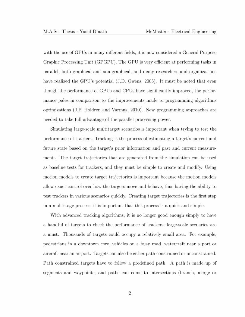
The goal of this thesis is to develop a method to simulate large-scale multitarget

scenarios, which takes advantage of the parallelization power provided by the Graph-

ical Processing Unit (GPU) in combination with the Central Processing Unit (CPU).

With this method and simulations, it will be shown how the combined use of GPU

and CPU to simulate scenarios is an improvement compared to using the CPU alone.

To simulate scenarios, the algorithm for the GPU will be broken down into a mul-

tistage process, showing exactly how to parallelize the CPU’s sequential process of

generating scenarios and showing the math behind the parallelized code.

The CPU’s performance has consistently improved, according to Moore’s Law,

based on clock frequency and the number of transistors. However, the CPU does

not only execute one algorithm, it also carries out instructions for the entire system.

GPU were initially designed for rapid processing for graphical output. With GPUs

becoming widely available, with dramatic improvements to computational speed and

1

M.A.Sc. Thesis - Yusuf Dinath McMaster - Electrical Engineering

with the use of GPUs in many different fields, it is now considered a General Purpose

Graphic Processing Unit (GPGPU). The GPU is very efficient at performing tasks in

parallel, both graphical and non-graphical, and many researchers and organizations

have realized the GPU’s potential (J.D. Owens, 2005). It must be noted that even

though the performance of GPUs and CPUs have significantly improved, the perfor-

mance pales in comparison to the improvements made to programming algorithms

optimizations (J.P. Holdren and Varmus, 2010). New programming approaches are

needed to take full advantage of the parallel processing power.

Simulating large-scale multitarget scenarios is important when trying to test the

performance of trackers. Tracking is the process of estimating a target’s current and

future state based on the target’s prior information and past and current measure-

ments. The target trajectories that are generated from the simulation can be used

as baseline tests for trackers, and they must be simple to create and modify. Using

motion models to create target trajectories is important because the motion models

allow exact control over how the targets move and behave, thus having the ability to

test trackers in various scenarios quickly. Creating target trajectories is the first step

in a multistage process; it is important that this process is a quick and simple.

With advanced tracking algorithms, it is no longer good enough simply to have

a handful of targets to check the performance of trackers; large-scale scenarios are

a must. Thousands of targets could occupy a relatively small area. For example,

pedestrians in a downtown core, vehicles on a busy road, watercraft near a port or

aircraft near an airport. Targets can also be either path constrained or unconstrained.

Path constrained targets have to follow a predefined path. A path is made up of

segments and waypoints, and paths can come to intersections (branch, merge or

2


cross) (T. Kirubarajan and Kadar, 2000). A path can be defined by one of many

motion models, and can have various restrictions, such as speed, acceleration, width,

etc. Constrained targets deviating from a path is a highly unlikely event, whereas

unconstrained targets can freely move in any direction without any restrictions.

For targets such as pedestrians, vehicles and short range watercraft, it is possible

to run simulations in a two-dimensional (2D) environment. A local coordinate system

is acceptable when using short-range targets. However, for long-range vessels such

as large watercraft or any aircraft, the curvature of the earth must be taken into

account. Therefore, the simulations must be generated in a three-dimensional (3D)

environment. The earth is best represented as a specialized ellipsoid, where the

distance from the North Pole to South Pole is shorter than the distance east to west.

To represent the earth as an ellipsoid, the World Geodetic System - 1984 (WGS-

84) standard is used. Using this standard, it is easy to plot targets trajectories in

Cartesian coordinates, or even have the target trajectories in geographic coordinates

(longitude, latitude and altitude). (ICAO, 2002)

The main contributions provided by this thesis are as follows:

• Parallelizing the target generation by parallelizing the motion legs:

There are multiple ways to generate target trajectories. The way presented in

this thesis is done by parallelizing a target’s motion legs; every element in the

motion leg is calculated at once.

• A new general state equation must be derived:

The state equation must be manipulated such that it can be run in parallel.

Adding noise to the non-Cartesian elements makes parallelizing the state equa-

tion difficult.

3


• The state vector xk is broken up into two separate parts:

One part of the state equation is for Cartesian elements and the other part is

for non-Cartesian elements (such as the turn rate, ω). It is assumed that the

state transition matrix is only dependent on the non-Cartesian elements.

The remainder of the thesis is structured as follows. Chapter 2 provides back-

ground information on other targets, coordinate systems, process noise and motion

models (in two-dimension and three-dimension space). Also discussed in Chapter 2 is

the problem that is being solved on the GPU and background mathematics needed for

target generation. Chapter 3 discusses GPUs in general, CUDA C and the best prac-

tices for programming in CUDA C. The scenario using only a CPU and the scenario

using both GPU and CPU are given in Chapter 4. Also, Chapter 4 briefly discusses

small and large scale target trajectories, large-scale motion models (LSMM) and path

constrained (with rotational matrix) and unconstrained targets. Chapter 4 also de-

scribes how the algorithm is implemented on the CPU and how it is implemented on

the GPU, and answers why in the GPU is one motion leg, instead of one target, being

generated at a time, and why not have each target generated in parallel. Chapter 4

ends with the breakdown of the CUDA kernel calls and the importance of the prefix

sum (scan) technique. Chapter 5 presents simulation results that demonstrate the

effectiveness of the proposed approaches. Conclusions, future work and applications

are presented in Chapter 6.

4


1.1 Related Publication

• Y. Dinath, T. Kirubarajan, R. Tharmarasa, P. Valin and E. Meger, “Simulation

of Large-Scale Multitarget Tracking Scenarios Using GPUs”, Proceedings of the

Signal and Data Processing of Small Targets, Baltimore, MD, May 2012.

5

Chapter 2

Target Generation

2.1 Targets

Targets are not limited to one type of object or thing. “Target” is applied ubiqui-

tously and to any object that demonstrates a dynamic motion; hence, the target is

represented by a point particle (infinitesimal dimensions) occupying a point in space.

The target’s dynamic motion helps identify what type of object the target is (Tewari,

2007). Some examples of targets are:

• Dismounted Combatants/Pedestrians: They have more mobility and have fewer

constraints, even when being restricted to paths. Pedestrians move with rel-

atively slow speeds, but can change direction quickly and without significant

change in acceleration or speed. Pedestrians are able to be modeled in either a

2D or 3D environment.

• Automobiles: Vehicles are more restricted to lanes and have speed limitations,

although they travel much faster than pedestrians. An automobile’s motion can

6


be limited to acceleration/deceleration, constant velocity and constant turn.

Automobiles are able to be modeled in either a 2D or 3D environment.

• Watercraft: There are wide varieties of watercraft, such as ships, boats and

submarines. Watercraft parameters, such as maximum speed, acceleration and

mobility, change depending on the type of watercraft. Watercraft can be mod-

eled in a 2D environment using a local coordinate system. For long distances,

it should be modeled in 3D to account for the earth’s curvature.

• Fixed-wing Aircraft: There are wide varieties of fixed-wing aircraft that usually

vary in size. To account for the earth’s curvature and because of the distances

and flight dynamics usually involved with aircraft, it is best that aircraft motion

be modeled only in a 3D environment using a global coordinate system.

If the target’s physical properties were considered, then the shape and size of

the target, its rotational motion and momentum changes would become important

when modelling a target. However, the focus of this thesis is on the simulation of

target trajectory, and the physical properties of said target are irrelevant. Therefore,

this leaves a target with either two or three degrees of freedom depending on the

environment. It can be assumed that the point particle is the target’s centre of mass.

(Galben, 2011)

A target’s motion model (refer to Section 2.3) describes how the target moves

through space with respect to time (Li and Jilkov, 2003).

Since the target is a point mass, it can be assumed that (Galben, 2011):

• the target is rigid

• the target rotates with the same angular speed

7


• there is no slippage - no loss of traction between the surface and target

2.2 Coordinate Systems

For the types of targets that will be looked at in this thesis, mainly (refer to Section

2.1) pedestrians, automobiles, watercraft and fixed-wing aircraft, their movements

would be best described in either the Cartesian coordinate system (refer to Subsec-

tion 2.2.1) or geographic coordinate system (refer to Subsection 2.2.2). The ideal

coordinate system depends on whether the target moves in either 2D or 3D space

and the distance the target has to traverse. If the target does not travel a significant

distance, then a local coordinates in 2D would be acceptable; otherwise, 3D space is

the preferred environment.

2.2.1 Cartesian Coordinates System

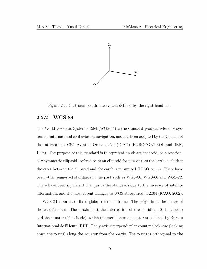
The Cartesian coordinate system is a typical coordinate system for both 2D and

3D space, where X, Y and Z, as per convention, are orientated relative to each

other using the right-hand rule. When generating, measuring or tracking targets, the

Cartesian coordinate system is generally used to define the position of pedestrians and

automobiles. The position of watercraft can be defined in the Cartesian coordinate

system on a small scale, where the curvature of the earth would not be a factor.

8


X

Y

Z

Figure 2.1: Cartesian coordinate system defined by the right-hand rule

2.2.2 WGS-84

The World Geodetic System - 1984 (WGS-84) is the standard geodetic reference sys-

tem for international civil aviation navigation, and has been adopted by the Council of

the International Civil Aviation Organization (ICAO) (EUROCONTROL and IfEN,

1998). The purpose of this standard is to represent an oblate spheroid, or a rotation-

ally symmetric ellipsoid (refered to as an ellipsoid for now on), as the earth, such that

the error between the ellipsoid and the earth is minimized (ICAO, 2002). There have

been other suggested standards in the past such as WGS-60, WGS-66 and WGS-72.

There have been significant changes to the standards due to the increase of satellite

information, and the most recent changes to WGS-84 occured in 2004 (ICAO, 2002).

WGS-84 is an earth-fixed global reference frame. The origin is at the centre of

the earth’s mass. The x-axis is at the intersection of the meridian (0◦ longitude)

and the equator (0◦ latitude), which the meridian and equator are defined by Bureau

International de l’Heure (BIH). The y-axis is perpendicular counter clockwise (looking

down the z-axis) along the equator from the x-axis. The z-axis is orthogonal to the

9


x-axis and y-axis pointing up. However, due to polar motion, the z-axis is not a true

representation of the earth’s rotational axis. The x-axis, y-axis and z-axis satisfy the

right-hand rule.

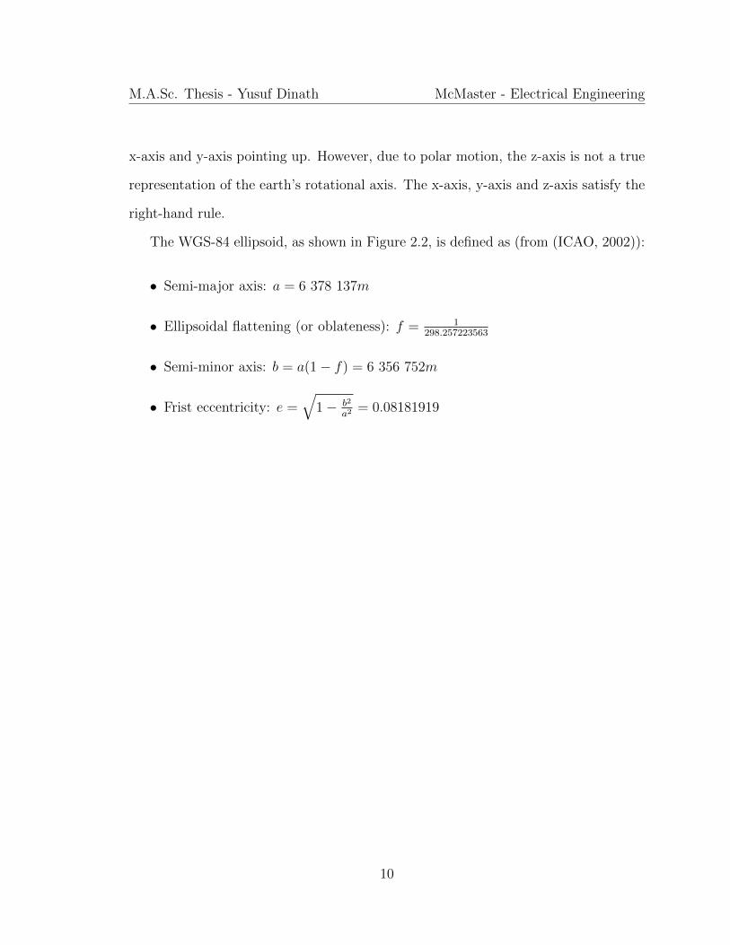
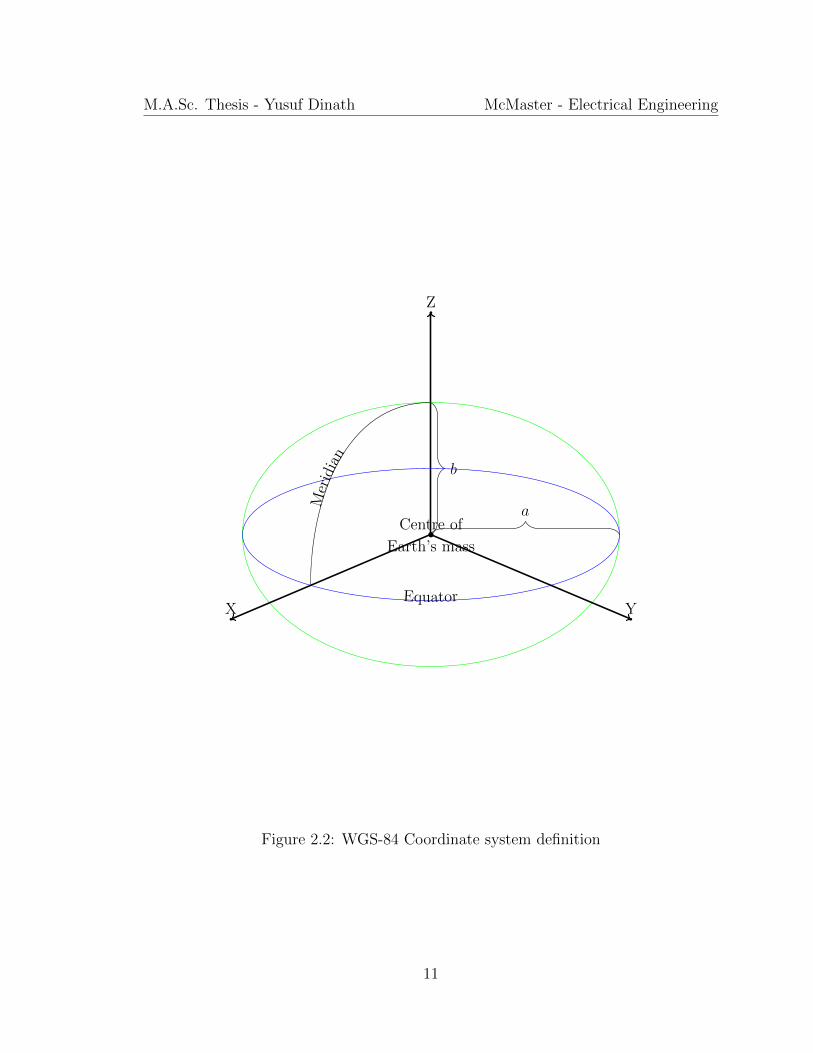
The WGS-84 ellipsoid, as shown in Figure 2.2, is defined as (from (ICAO, 2002)):

• Semi-major axis: a = 6 378 137m

• Ellipsoidal flattening (or oblateness): f = 1298.257223563

• Semi-minor axis: b = a(1− f) = 6 356 752m

• Frist eccentricity: e =√

1− b2

a2= 0.08181919

10


X Y

Z

b

aMer

idia

n

Equator

Centre of

Earth’s mass

Figure 2.2: WGS-84 Coordinate system definition

11


2.2.3 ECEF

Earth-Centered, Earth-Fixed is a Cartesian coordinates system (refer to Subsection

2.2.1), where the origin, (0,0,0), represents the earth’s centre of mass. Similar to

WGS-84 (refer to Subsection 2.2.2), the x-axis is through the meridian and the equa-

tor, the y-axis is perpendicular counter clockwise (looking down the z-axis) horizon-

tally from the x-axis, and the z-axis is orthogonal to the x-axis and y-axis pointing

up. The x-axis, y-axis and z-axis satisfy the right-hand rule convention. (EURO-

CONTROL and IfEN, 1998)

2.3 Motion Models

The state equation is assumed to be of the following form (Li and Jilkov, 2003):

xk = Fkxk−1 +Gkνk (2.1)

where, at time step k, xk is the current state, Fk is the state transition matrix, Gk is

the gain matrix for the independent white noise vector, νk.

12


2.3.1 Non-Maneuvering Targets

The Constant Velocity model is a well-known model for non-maneuvering targets (Li

and Jilkov, 2003):

xk =

x

x

y

y

Fk =

1 T 0 0

0 1 0 0

0 0 1 T

0 0 0 1

Gk =

T 2

20

T 0

0 T 2

2

0 T

(2.2)

where x and y are the standard Cartesian coordinates in 2D space, x and y represents

the velocity along each dimension and T is the target motion sample duration. T is

defined as the time difference between k and (k − 1).

2.3.2 Maneuvering Targets

The Constant Turn model is also a well-known model but for maneuvering targets

(Li and Jilkov, 2003):

xk =

x

x

y

y

ω

Fk =

1 sinωTω

0 −(1−cosωT )ω

0

0 cosωT 0 − sinωT 0

0 1−cosωTω

1 sinωTω

0

0 sinωT 0 cosωT 0

0 0 0 0 1

Gk =

T 2

20 0

T 0 0

0 T 2

20

0 T 0

0 0 T

(2.3)

where ω is the turn rate.

13


Other models that can be used are: Weiner Sequence Acceleration, Singer Accel-

eration, White Noise Jerk, Constant Turn with Cartesian Velocity, found in (Li and

Jilkov, 2003). It is important to note that turn models are dependent on ω, and ω

changes after each time step because of noise.

2.3.3 3D Models

For watercraft and aircraft type targets that traverse long distances, it is best to model

the targets using the WGS-84 stantard earth model (refer to Subsection 2.2.2).

The motion can be broken down into two components: motion in the vertical

plane and motion in the horizontal plane. Using the equations from (Galben, 2011):

xk = xk−1 −[Rmk−1 cosφk−1 −Rm

k cos (φk−1 + φkT )]

cosλk−1︸︷︷︸Vertical Plane

−[Rvk−1 cosλk−1 −Rv

k cos (λk−1 + λkT )]

︸︷︷︸Horizontal Plane

yk = yk−1 −[Rmk−1 cosφk−1 −Rm

k cos (φk−1 + φkT )]

sinλk−1︸︷︷︸Vertical Plane

−[Rvk−1 sinλk−1 −Rv

k sin (λk−1 + λkT )]

︸︷︷︸Horizontal Plane

zk = zk−1 −[Rmk−1 sinφk−1 −Rm

k sin (φk−1 + φkT )]

where Rv is the radii of curvature in the prime vertical, Rm is the radii of curvature

in the meridian, and φ and λ are the latitude and longitudinal velocity, respectively,

14


in radians per unit time. From (Sankowski, 2011)), Rv, Rm, φ and λ are defined as:

Rvk =

a√1− e2 sin2 φk

Rmk =

a(1− e2)(1− e2 sin2 φk)

32

λk =υλk

Rvk cosφ

φk =υφkRmk

υφk and υλk is the ground velocity for latitude and longitude, respectively.

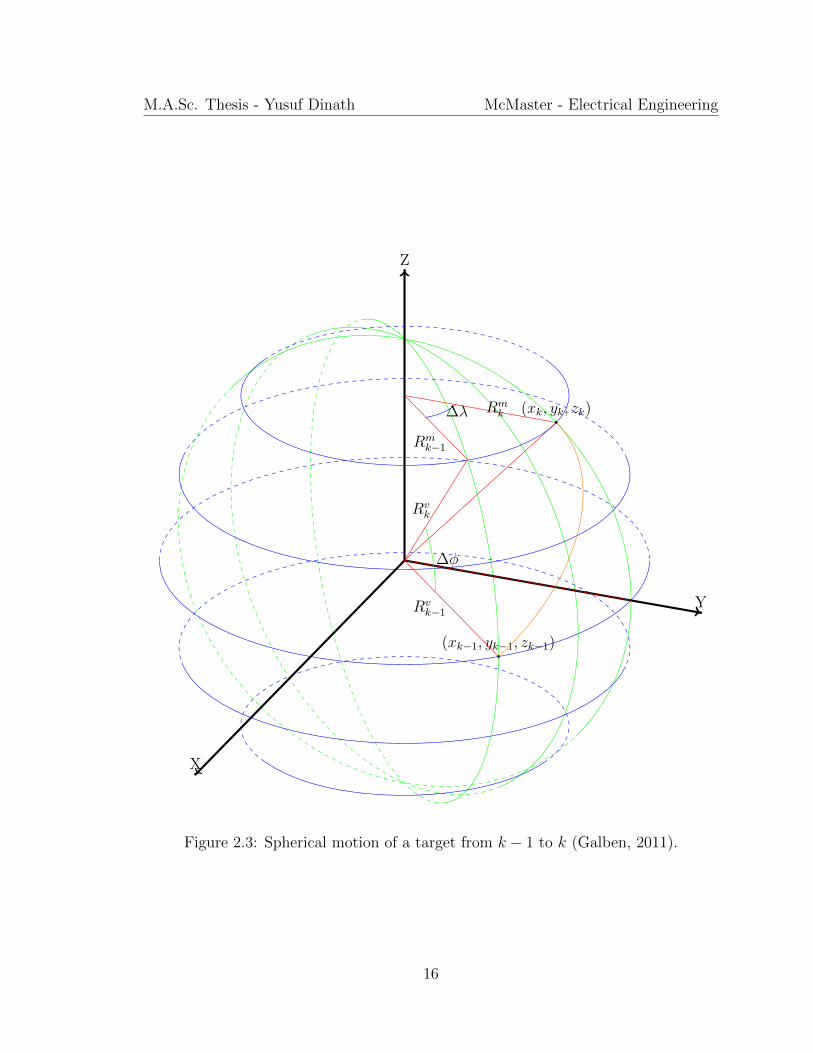
Figure 2.3 displays an example of the Earth, where a target is starting at the coor-

dinate at (xk−1, yk−1, zk−1) and following a great circle to the coordinate at (xk, yk, zk).

15


X

Y

Z

(xk−1, yk−1, zk−1)

(xk, yk, zk)

∆φ

∆λ

Rvk−1

Rvk

Rmk−1

Rmk

Figure 2.3: Spherical motion of a target from k − 1 to k (Galben, 2011).

16


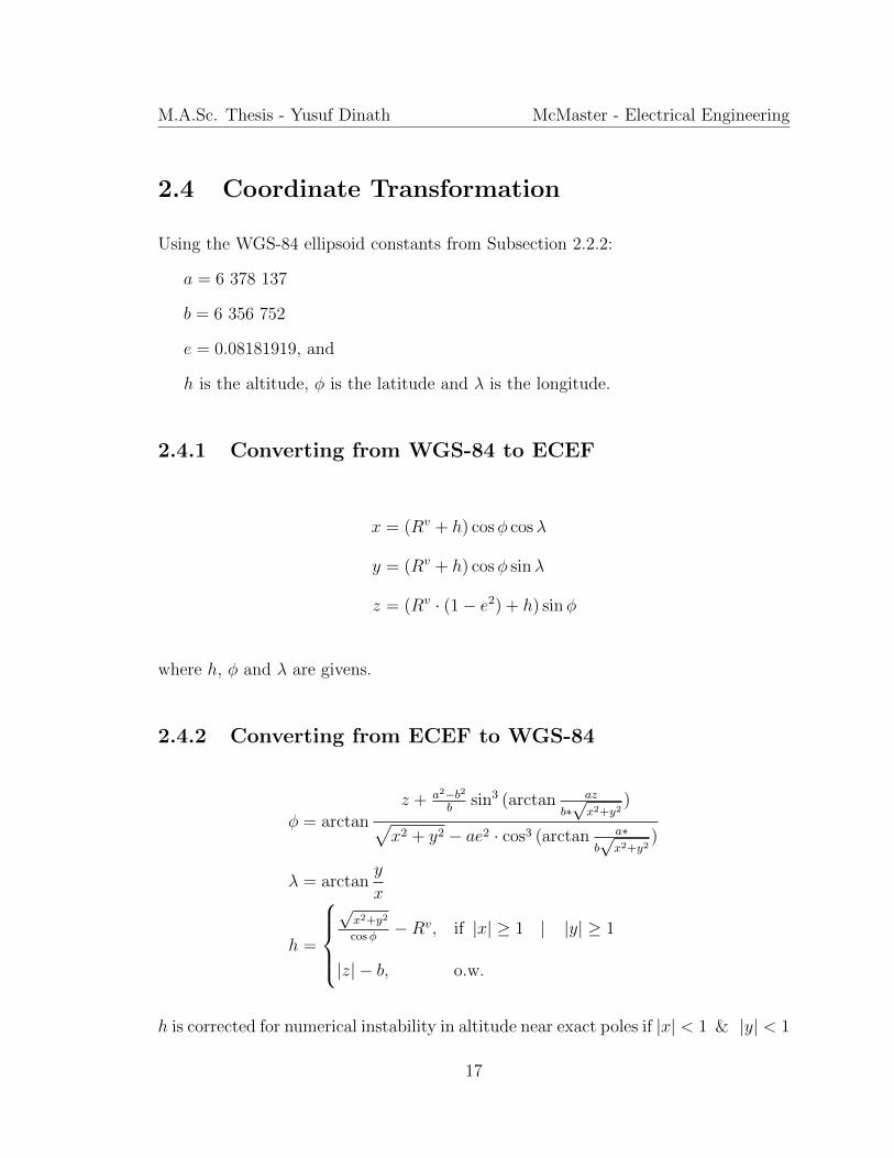
2.4 Coordinate Transformation

Using the WGS-84 ellipsoid constants from Subsection 2.2.2:

a = 6 378 137

b = 6 356 752

e = 0.08181919, and

h is the altitude, φ is the latitude and λ is the longitude.

2.4.1 Converting from WGS-84 to ECEF

x = (Rv + h) cosφ cosλ

y = (Rv + h) cosφ sinλ

z = (Rv · (1− e2) + h) sinφ

where h, φ and λ are givens.

2.4.2 Converting from ECEF to WGS-84

φ = arctanz + a2−b2

bsin3 (arctan az

b∗√x2+y2

)√x2 + y2 − ae2 · cos3 (arctan a∗

b√x2+y2

)

λ = arctany

x

h =

√x2+y2

cosφ−Rv, if |x| ≥ 1 | |y| ≥ 1

|z| − b, o.w.

h is corrected for numerical instability in altitude near exact poles if |x| < 1 & |y| < 1

17


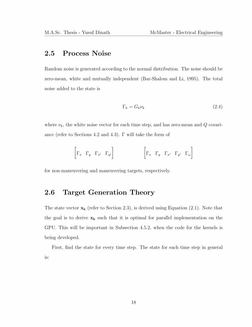
2.5 Process Noise

Random noise is generated according to the normal distribution. The noise should be

zero-mean, white and mutually independent (Bar-Shalom and Li, 1995). The total

noise added to the state is

Γk = Gkνk (2.4)

where νk, the white noise vector for each time step, and has zero-mean and Q covari-

ance (refer to Sections 4.2 and 4.3). Γ will take the form of

[Γx Γy Γx′ Γy′

] [Γx Γy Γx′ Γy′ Γω

]

for non-maneuvering and maneuvering targets, respectively.

2.6 Target Generation Theory

The state vector xk (refer to Section 2.3), is derived using Equation (2.1). Note that

the goal is to derive xk such that it is optimal for parallel implementation on the

GPU. This will be important in Subsection 4.5.2, when the code for the kernels is

being developed.

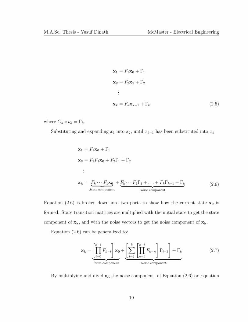
First, find the state for every time step. The state for each time step in general

is:

18


x1 = F1x0 + Γ1

x2 = F2x1 + Γ2

...

xk = Fkxk−1 + Γk (2.5)

where Gk ∗ νk = Γk.

Substituting and expanding x1 into x2, until xk−1 has been substituted into xk

x1 = F1x0 + Γ1

x2 = F2F1x0 + F2Γ1 + Γ2

...

xk = Fk · · ·F1x0︸︷︷︸State component

+Fk · · ·F2Γ1 + . . .+ FkΓk−1 + Γk︸︷︷︸Noise component

(2.6)

Equation (2.6) is broken down into two parts to show how the current state xk is

formed. State transition matrices are multiplied with the initial state to get the state

component of xk, and with the noise vectors to get the noise component of xk.

Equation (2.6) can be generalized to:

xk =

[k−1∏i=0

Fk−i

]x0︸︷︷︸

State component

+

[k∑i=2

[k−i∏n=0

Fk−n

]Γi−1

]+ Γk︸︷︷︸

Noise component

(2.7)

By multiplying and dividing the noise component, of Equation (2.6) or Equation

19


(2.7), with Fk · · ·F1, helps to parallelize the state equation.

(F1)−1Γ1 + . . .+ (Fk−1 · · ·F1)

−1Γk−1 + (Fk · · ·F1)−1Γk (2.8)

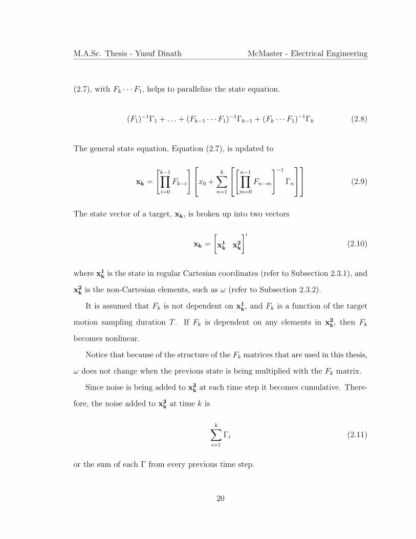
The general state equation, Equation (2.7), is updated to

xk =

[k−1∏i=0

Fk−i

]x0 +k∑

n=1

[n−1∏m=0

Fn−m

]−1Γn

(2.9)

The state vector of a target, xk, is broken up into two vectors

xk =

[x1k x2

k

]′(2.10)

where x1k is the state in regular Cartesian coordinates (refer to Subsection 2.3.1), and

x2k is the non-Cartesian elements, such as ω (refer to Subsection 2.3.2).

It is assumed that Fk is not dependent on x1k, and Fk is a function of the target

motion sampling duration T . If Fk is dependent on any elements in x2k, then Fk

becomes nonlinear.

Notice that because of the structure of the Fk matrices that are used in this thesis,

ω does not change when the previous state is being multiplied with the Fk matrix.

Since noise is being added to x2k at each time step it becomes cumulative. There-

fore, the noise added to x2k at time k is

k∑i=1

Γi (2.11)

or the sum of each Γ from every previous time step.

20

Chapter 3

GPU Programming

3.1 GPU

The Graphical Processing Unit (GPU) was initially designed to calculate values for

computer graphics, so as to take an immense load off the CPU. This left the CPU

available to perform its other necessary calculations and to control logic flow. Now,

every modern personal computer (PC) has a GPU. A GPU that exceeds the parallel

processing power of a CPU; [processing power that is now being sought by the scien-

tific community, and being applied to applications other than just computer graphics.

(Fung and Mann, 2004)

A General Purpose Graphical Processing Unit (GPGPU) is when the GPU is used

for a general purpose, other than its typical processes, such as for computer graphics

(J.D. Owens, 2005). However, there are trade-offs and bottlenecks that need to be

considered. Is it worth the cost (in terms of time) to send data to and from the CPU

to the GPU? Can a sequential task be sufficiently parallelized such that it can run ef-

fectively and efficiently on a GPU? (Fung and Mann, 2004). It has been demonstrated

21


in the scientific community that a GPU performing computationally expensive tasks

does so more efficiently than a CPU. The GPU is designed for intensive computa-

tion, so it is imperative that the CPU and GPU work together when parallelizing a

program (Kirk and Hwu, 2010).

Although GPUs are now common, it is still difficult to program them effectively.

Sequential algorithms must be redesigned to be parallel and algorithms have to be

scalable.

3.2 CUDA

Compute Unified Device Architecture (CUDA), developed by NVIDIA, is an architec-

ture for GPGPU programming. NVIDIA created their own set of rules and extensions

that allow developers to write programs using the common C Programming language.

(NVIDIA, 2011)

CUDA has a scalable parallel programming model that can be developed in a

C/C++ programming environment. The programming environment is heterogeneous,

meaning it allows the user to code both CPU and GPU (serial and parallel) in a single

environment. The CUDA C programming environment allows the programmer to let

the parallel algorithms be their primary concern, and not have to worry about the

backend. Also, CUDA C programs are scalable, allowing the algorithm to be used on

many different GPUs (NVIDIA, 2011).

22


3.3 CUDA C Programming

Some definitions are important when programming in CUDA C. The host is the CPU

and the device is the GPU. Code is broken up into two parts: host code and device

code. The host calls the device by calling a kernel function. Only code in the kernel

function is executed in parallel. Mandatory inputs for the kernel are the number of

blocks and the number of threads, and shared memory is an optional input (NVIDIA,

2011).

Inside a grid is a group of blocks, and inside each block is a group of threads

(NVIDIA, 2011). A group of 32 threads is called a warp. It is important to have mul-

tiples of 32 threads inside each block for performance reasons. It is also important that

each thread inside a warp do exactly the same thing (no branch divergence)(NVIDIA,

2012).

Blocks are independent, and run asynchronously, but they can never be synchro-

nized within the kernel. Blocks have to be synchronised outside the kernel. The

block’s independence is what makes programs scalable. Threads run asynchronously,

but can be synchronized within the kernel at the cost of time. (NVIDIA, 2011)

3.3.1 Memory

The CPU and GPU have different memory spaces, and data is transferred through

the PCIe bus using CUDA APIs (NVIDIA, 2011).

There are a couple of important types of memory (not a complete list) (from

(NVIDIA, 2011))

Global memory:

• resides in device memory

23


• shared between blocks

• the size of a block can be 32, 64 or 128 bytes

• blocks are aligned into multiples of 32, 64 or 128 bytes

Shared memory:

• much faster accessing than global memory, and best to replace global with

shared memory in the kernel

• each block has its own shared memory

– shared memory in one block cannot be accessed in a different block

• best for each thread to access different banks, or

• best for every thread to access one bank

Using page-locked or pinned host memory eliminates any need for CPU and GPU

data transferred. Page-locked memory is a limited resource and only should be used

when there is a need to transfer large amounts of data to and from the host and

device (NVIDIA, 2011).

3.3.2 Toolkit

Initially released in June 2007, the toolkit has gone through thirteen other releases

to date, which have included many advances to make parallel programming easier

and faster. Most recently, NVIDIA have released a new complier that makes CUDA

programs faster. (NVIDIA, 2011)

24


The toolkit is what enables developers to program in C/C++ to create GPU-

accelerated programs. It includes a debugger and tips to optimize, guides and API

reference (NVIDIA, 2011).

3.3.3 Libraries

There are many different GPU-accelerated libraries available for CUDA, such as fast

Fourier transform library, sparse matrix library and others for high performance math

routines (NIVIDA, 2012).

The runtime APIs are implemented in the cudart dynamic library. Some of the

typical functions found in the cudart library are: cudaGetDeviceProperties(),

which gets the GPU properties; cudaMalloc() and cudaFree(), which allocate and

deallocate memory; and cudaMemcpy(), which transfers memory to and from the

host and device, and also transfers between different variables on the device. cu-

daHostAlloc() and cudaFreeHost() allocates and frees, respectively, page-locked

memory. cudaHostRegister() page-locks a range of memory allocated by malloc()

(NVIDIA, 2011).

The library that is used in Section 4.5 is the CURAND Library. This library is

used to generate a large set of normally distributed numbers, with zero mean and a

standard deviation of one (NVIDIA, 2011).

3.4 CUDA and the Best Practices

The CUDA C Best Practices Guide has highlighted some important issues to consider

when programming on the GPU (NVIDIA, 2012). It is important to consider these

25


issues when programming on CUDA.

One of the most important things to do before coding is to identify the different

ways to parallelize sequential code. If there are not many parts of the code that

can be parallelized, it may not be worth it to parallelize a small algorithm. One

reason is because of the bandwidth. The bandwidth is defined as the rate of data

transfer, and can be used as a performance measurement. It is very costly, in terms

of time, to transfer data from the host to the device and then back again. Therefore,

the number of host and device transfers must be minimized; otherwise, there may

be no gains in performance when executing code on the device compared to the

host. Once the memory is on the device, what type of memory is used and how it

is accessed is important. For example, it is always preferable to use shared memory

over global memory, because it is more expensive to access global memory than it

is to access shared memory. It is advised to copy memory from global memory into

shared memory to avoid calling global memory more times than necessary (NVIDIA,

2011).

Because of how the GPU is designed, it is best to have the number of threads in a

block of 32 for efficiency. As well, it is important to have all the threads in the warp

execute the same path; otherwise, thread divergence happens and will increase the

simulation run time (NVIDIA, 2011).

A few other miscellaneous items to keep in mind are: use unsigned integers as loop

counters, shift operations for multiplying and dividing and use “#pragma unroll” for

loops (NVIDIA, 2011).

26

Chapter 4

CPU and GPU Simulation

4.1 Target Trajectories

In order to create a simulation there are a few main parameters that need to be

defined, such as

• The number of Monte Carlo runs (Mm)

• The number of targets (L) (can be randomly generated at the start)

• The number of motion legs of a target (ML) (can also be randomly generated

at the start)

• The initial state, x0, for each target

• The F , G, (refer to Section 2.3) and the process noise covariance (refer to

Section 2.5) for each motion leg

Each Monte Carlo run is independent of each other. Each target is independent

of each other. However, elements in a motion leg are not independent of each other

because of noise. With this, it is possible to generate the state for each target at

27


every time step. For both the CPU and GPU, the processing power varies with Mm,

L, ML and the number of elements in each motion leg.

When implementing code for target generation on the GPU, two approaches can

be taken. The first approach, the one implemented in this thesis (refer to Section

4.5), is to generate the entire motion leg for every target in parallel. The second

approach is to generate every target in parallel. When writing a parallel algorithm,

there are various things to consider, such as the number of targets and the number

of elements in each motion leg.

For it to be possible to generate the entire motion leg in parallel on the GPU two

assumptions must be made. The first assumption is that Fk can only be a function

of x2k and not of x1

k (refer to Equation (2.10)). The second assumption is that any

element in x2k, such as a turn rate, will not change when the Fk matrix is multiplied

with the state matrix and will only change because of noise added.

There are two possibles methods that the user can use to create large-scale motion

models. The first method is with unconstrained targets, and the second method is

by constraining targets.

4.2 Large-Scale Motion Models with Path Uncon-

strained Targets

Unconstrained targets have almost every parameter randomly generated, including,

but not limited to the number of targets, the number of motion legs per target,

the initial state of the target, and the type of motion that the target will have.

Unconstrained targets do not have to follow any path and are free to move in any

28


direction.

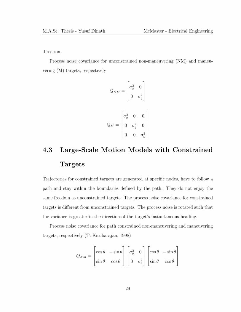
Process noise covariance for unconstrained non-maneuvering (NM) and maneu-

vering (M) targets, respectively

QNM =

σ2x 0

0 σ2y

QM =

σ2x 0 0

0 σ2y 0

0 0 σ2ω

4.3 Large-Scale Motion Models with Constrained

Targets

Trajectories for constrained targets are generated at specific nodes, have to follow a

path and stay within the boundaries defined by the path. They do not enjoy the

same freedom as unconstrained targets. The process noise covariance for constrained

targets is different from unconstrained targets. The process noise is rotated such that

the variance is greater in the direction of the target’s instantaneous heading.

Process noise covariance for path constrained non-maneuvering and maneuvering

targets, respectively (T. Kirubarajan, 1998)

QNM =

cos θ − sin θ

sin θ cos θ

σ2

o 0

0 σ2a

cos θ − sin θ

sin θ cos θ

29


QM =

cos θ − sin θ 0

sin θ cos θ 0

0 0 1

σ2o 0 0

0 σ2a 0

0 0 σ2ω

cos θ − sin θ 0

sin θ cos θ 0

0 0 1

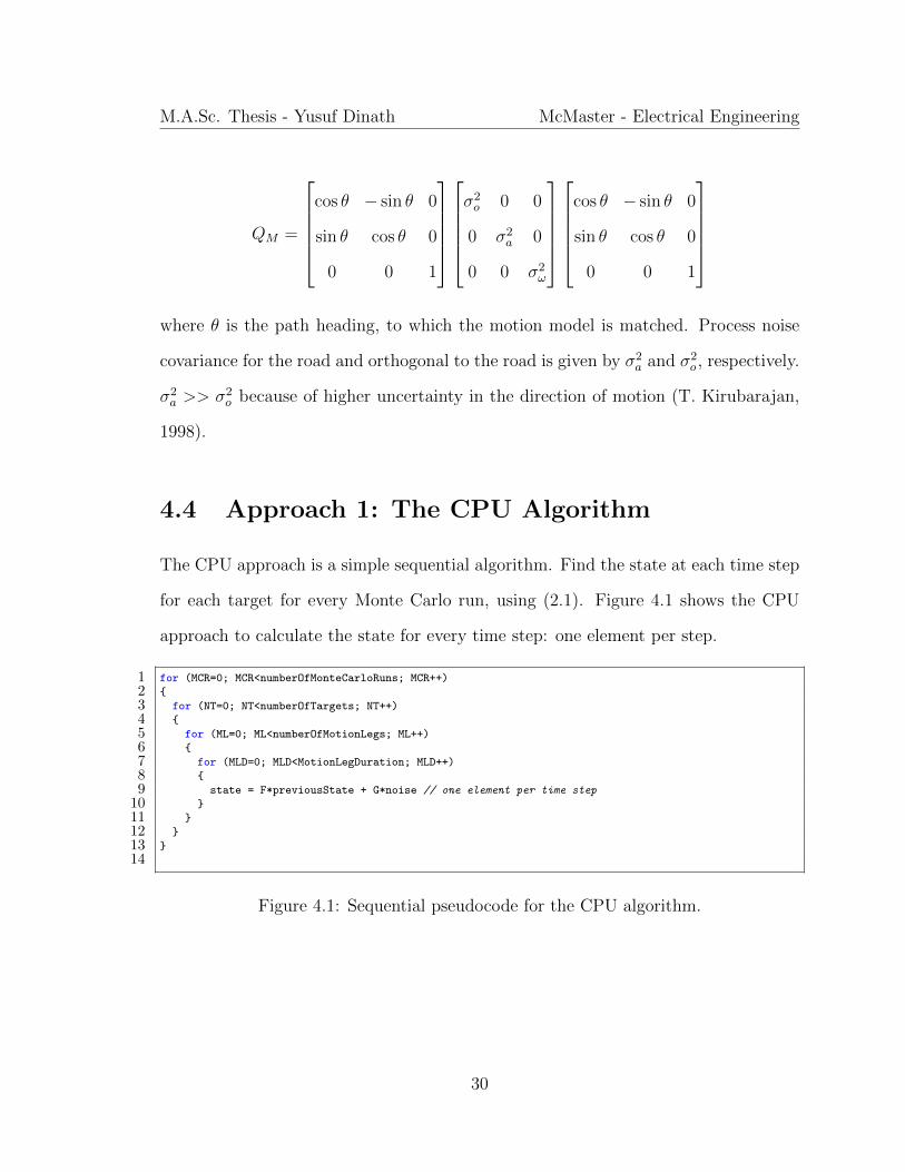
where θ is the path heading, to which the motion model is matched. Process noise

covariance for the road and orthogonal to the road is given by σ2a and σ2

o , respectively.

σ2a >> σ2

o because of higher uncertainty in the direction of motion (T. Kirubarajan,

1998).

4.4 Approach 1: The CPU Algorithm

The CPU approach is a simple sequential algorithm. Find the state at each time step

for each target for every Monte Carlo run, using (2.1). Figure 4.1 shows the CPU

approach to calculate the state for every time step: one element per step.

1 for (MCR=0; MCR<numberOfMonteCarloRuns; MCR++)

2 {

3 for (NT=0; NT<numberOfTargets; NT++)

4 {

5 for (ML=0; ML<numberOfMotionLegs; ML++)

6 {

7 for (MLD=0; MLD<MotionLegDuration; MLD++)

8 {

9 state = F*previousState + G*noise // one element per time step

10 }

11 }

12 }

13 }

14

Figure 4.1: Sequential pseudocode for the CPU algorithm.

30


4.5 Approach 2: The GPU Algorithm

For the GPU approach, it is not just simply a matter of taking the CPU approach and

generating that in parallel. Refer to Section 3.4 for reasons why. Figure 4.2 shows

the GPU approach to calculate the state for every time step: all at once.

1 for (MCR=0; MCR<numberOfMonteCarloRuns; MCR++)

2 {

3 for (NT=0; NT<numberOfTargets; NT++)

4 {

5 for (ML=0; ML<numberOfMotionLegs; ML++)

6 {

7 state = F*previousState + G*noise // every element in the motion leg at once

8 }

9 }

10 }

11

Figure 4.2: Motion Leg Parallelization pseudocode for the GPU algorithm.

4.5.1 Parallel Prefix Sum (Scan) with CUDA

The scan with CUDA is an important technique to implement (2.9). Simply doing a

scan with an array of k elements,

a0 a1 a2 a3 a4 a5 . . . ak

returns

I a0 a0⊕

...⊕

a1 a0⊕

...⊕

a2 a0⊕

...⊕

a3 a0⊕

...⊕

a4 . . . a0⊕...

⊕ak−2

where I is the identity matrix and⊕

is the binary associative operator (Harris, 2008).

31


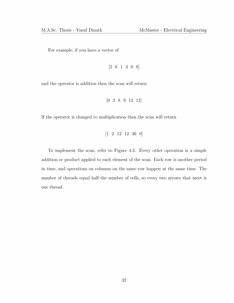
For example, if you have a vector of

[2 6 1 3 0 8]

and the operator is addition then the scan will return

[0 2 8 9 12 12]

If the operator is changed to multiplication then the scan will return

[1 2 12 12 36 0]

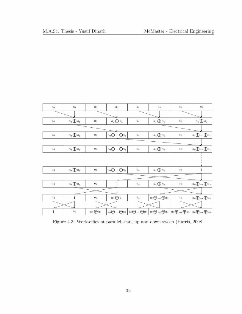
To implement the scan, refer to Figure 4.3. Every other operation is a simple

addition or product applied to each element of the scan. Each row is another period

in time, and operations on columns on the same row happen at the same time. The

number of threads equal half the number of cells, so every two arrows that meet is

one thread.

32


a0 a1 a2 a3 a4 a5 a6 a7

a0 a0⊕

a1 a2 a2⊕

a3 a4 a4⊕

a5 a6 a6⊕

a7

a0 a0⊕

a1 a2 a0⊕

...⊕a3 a4 a4

⊕a5 a6 a4

⊕...⊕a7

a0 a0⊕

a1 a2 a0⊕

...⊕a3 a4 a4

⊕a5 a6 a0

⊕...⊕a7

a0 a0⊕

a1 a2 a0⊕

...⊕a3 a4 a4

⊕a5 a6 I

a0 a0⊕

a1 a2 I a4 a4⊕

a5 a6 a0⊕

...⊕a3

a0 I a2 a0⊕

a1 a4 a0⊕

...⊕a3 a6 a0

⊕...⊕a5

I a0 a0⊕

a1 a0⊕

...⊕a2 a0

⊕...⊕a3 a0

⊕...⊕a4 a0

⊕...⊕a5 a0

⊕...⊕a6

Figure 4.3: Work-efficient parallel scan, up and down sweep (Harris, 2008)

33


4.5.2 Kernel

In CUDA C, the kernel is a function that executes device code; invokes the device.

Anything in the kernel gets compiled for the device and everything else is compiled

for the host (Sanders and Kandrot, 2011).

The code needs to be broken down into four kernels. This is necessary when

motion legs are broken up several times depending on how many GPU blocks are

created. Blocks have to be synchronized, but this can only happen from within the

host, and cannot happen from within the kernel.

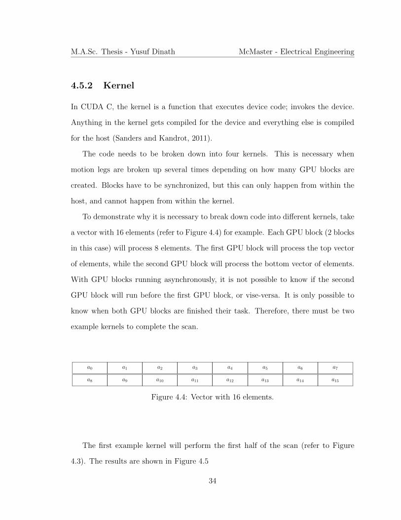
To demonstrate why it is necessary to break down code into different kernels, take

a vector with 16 elements (refer to Figure 4.4) for example. Each GPU block (2 blocks

in this case) will process 8 elements. The first GPU block will process the top vector

of elements, while the second GPU block will process the bottom vector of elements.

With GPU blocks running asynchronously, it is not possible to know if the second

GPU block will run before the first GPU block, or vise-versa. It is only possible to

know when both GPU blocks are finished their task. Therefore, there must be two

example kernels to complete the scan.

a0 a1 a2 a3 a4 a5 a6 a7

a8 a9 a10 a11 a12 a13 a14 a15

Figure 4.4: Vector with 16 elements.

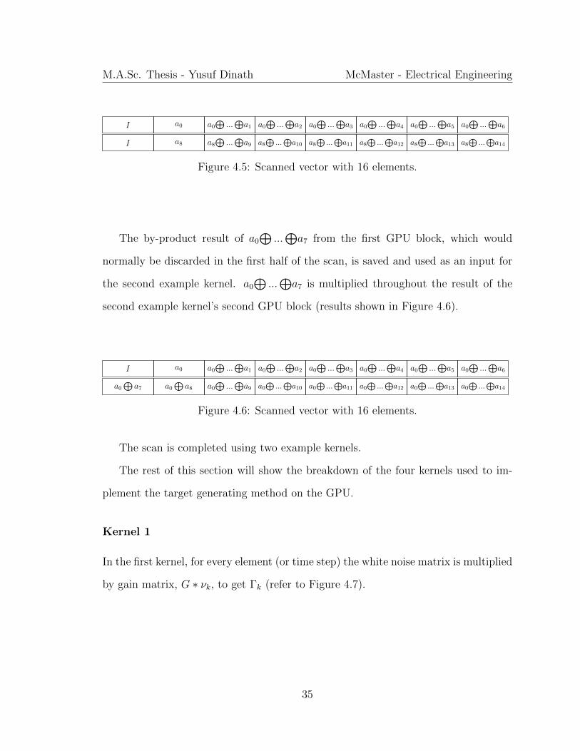
The first example kernel will perform the first half of the scan (refer to Figure

4.3). The results are shown in Figure 4.5

34


I a0 a0⊕

...⊕a1 a0

⊕...⊕a2 a0

⊕...⊕a3 a0

⊕...⊕a4 a0

⊕...⊕a5 a0

⊕...⊕a6

I a8 a8⊕

...⊕a9 a8

⊕...⊕

a10 a8⊕

...⊕

a11 a8⊕

...⊕

a12 a8⊕

...⊕

a13 a8⊕

...⊕

a14

Figure 4.5: Scanned vector with 16 elements.

The by-product result of a0⊕

...⊕a7 from the first GPU block, which would

normally be discarded in the first half of the scan, is saved and used as an input for

the second example kernel. a0⊕

...⊕a7 is multiplied throughout the result of the

second example kernel’s second GPU block (results shown in Figure 4.6).

I a0 a0⊕

...⊕a1 a0

⊕...⊕a2 a0

⊕...⊕a3 a0

⊕...⊕a4 a0

⊕...⊕a5 a0

⊕...⊕a6

a0⊕

a7 a0⊕

a8 a0⊕

...⊕a9 a0

⊕...⊕

a10 a0⊕

...⊕

a11 a0⊕

...⊕

a12 a0⊕

...⊕

a13 a0⊕

...⊕

a14

Figure 4.6: Scanned vector with 16 elements.

The scan is completed using two example kernels.

The rest of this section will show the breakdown of the four kernels used to im-

plement the target generating method on the GPU.

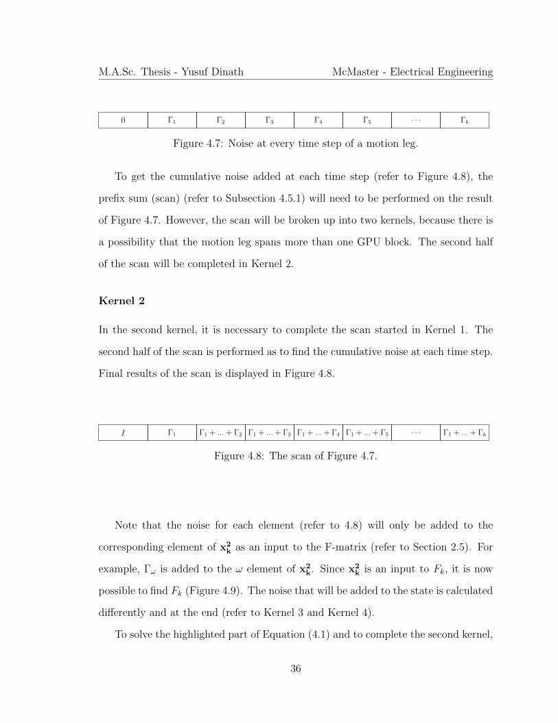
Kernel 1

In the first kernel, for every element (or time step) the white noise matrix is multiplied

by gain matrix, G ∗ νk, to get Γk (refer to Figure 4.7).

35


0 Γ1 Γ2 Γ3 Γ4 Γ5. . . Γk

Figure 4.7: Noise at every time step of a motion leg.

To get the cumulative noise added at each time step (refer to Figure 4.8), the

prefix sum (scan) (refer to Subsection 4.5.1) will need to be performed on the result

of Figure 4.7. However, the scan will be broken up into two kernels, because there is

a possibility that the motion leg spans more than one GPU block. The second half

of the scan will be completed in Kernel 2.

Kernel 2

In the second kernel, it is necessary to complete the scan started in Kernel 1. The

second half of the scan is performed as to find the cumulative noise at each time step.

Final results of the scan is displayed in Figure 4.8.

I Γ1 Γ1 + ...+ Γ2 Γ1 + ...+ Γ3 Γ1 + ...+ Γ4 Γ1 + ...+ Γ5. . . Γ1 + ...+ Γk

Figure 4.8: The scan of Figure 4.7.

Note that the noise for each element (refer to 4.8) will only be added to the

corresponding element of x2k as an input to the F-matrix (refer to Section 2.5). For

example, Γω is added to the ω element of x2k. Since x2

k is an input to Fk, it is now

possible to find Fk (Figure 4.9). The noise that will be added to the state is calculated

differently and at the end (refer to Kernel 3 and Kernel 4).

To solve the highlighted part of Equation (4.1) and to complete the second kernel,

36


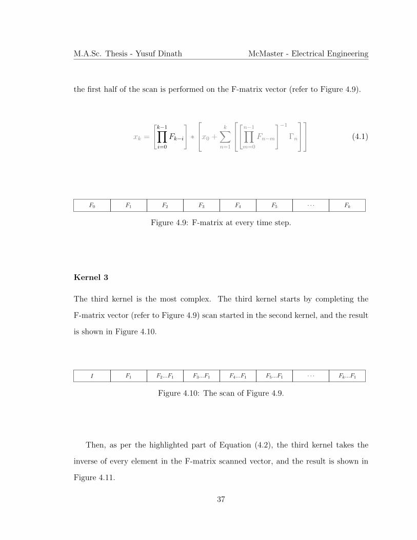
the first half of the scan is performed on the F-matrix vector (refer to Figure 4.9).

xk =

[k−1∏i=0

Fk−i

]∗

x0 +k∑

n=1

[n−1∏m=0

Fn−m

]−1Γn

(4.1)

F0 F1 F2 F3 F4 F5. . . Fk

Figure 4.9: F-matrix at every time step.

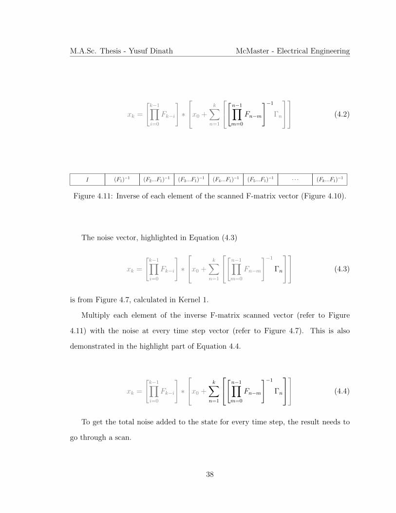
Kernel 3

The third kernel is the most complex. The third kernel starts by completing the

F-matrix vector (refer to Figure 4.9) scan started in the second kernel, and the result

is shown in Figure 4.10.

I F1 F2...F1 F3...F1 F4...F1 F5...F1. . . Fk...F1

Figure 4.10: The scan of Figure 4.9.

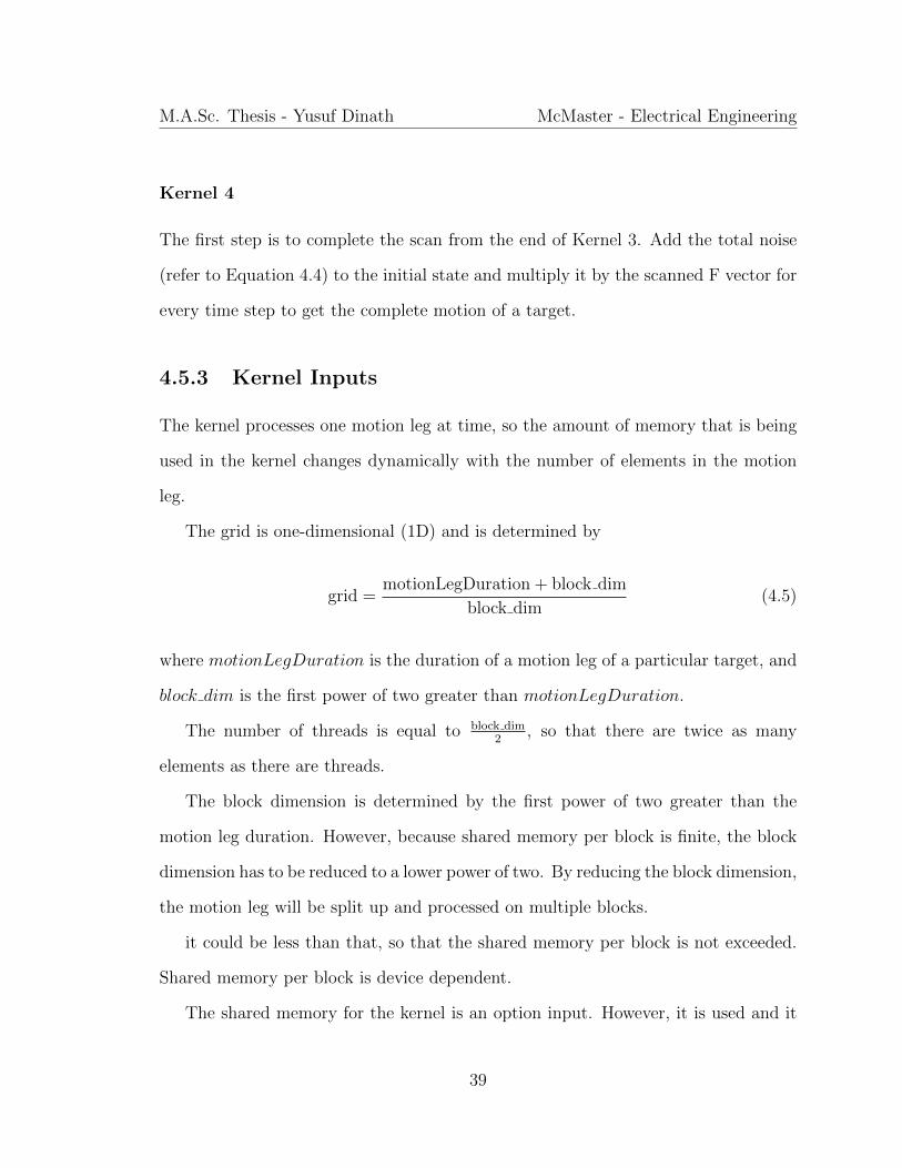
Then, as per the highlighted part of Equation (4.2), the third kernel takes the

inverse of every element in the F-matrix scanned vector, and the result is shown in

Figure 4.11.

37


xk =

[k−1∏i=0

Fk−i

]∗

x0 +k∑

n=1

[n−1∏m=0

Fn−m

]−1Γn

(4.2)

I (F1)−1 (F2...F1)

−1 (F3...F1)−1 (F4...F1)

−1 (F5...F1)−1 . . . (Fk...F1)

−1

Figure 4.11: Inverse of each element of the scanned F-matrix vector (Figure 4.10).

The noise vector, highlighted in Equation (4.3)

xk =

[k−1∏i=0

Fk−i

]∗

x0 +k∑

n=1

[n−1∏m=0

Fn−m

]−1Γn

(4.3)

is from Figure 4.7, calculated in Kernel 1.

Multiply each element of the inverse F-matrix scanned vector (refer to Figure

4.11) with the noise at every time step vector (refer to Figure 4.7). This is also

demonstrated in the highlight part of Equation 4.4.

xk =

[k−1∏i=0

Fk−i

]∗

x0 +k∑

n=1

[n−1∏m=0

Fn−m

]−1Γn

(4.4)

To get the total noise added to the state for every time step, the result needs to

go through a scan.

38


Kernel 4

The first step is to complete the scan from the end of Kernel 3. Add the total noise

(refer to Equation 4.4) to the initial state and multiply it by the scanned F vector for

every time step to get the complete motion of a target.

4.5.3 Kernel Inputs

The kernel processes one motion leg at time, so the amount of memory that is being

used in the kernel changes dynamically with the number of elements in the motion

leg.

The grid is one-dimensional (1D) and is determined by

grid =motionLegDuration + block dim

block dim(4.5)

where motionLegDuration is the duration of a motion leg of a particular target, and

block dim is the first power of two greater than motionLegDuration.

The number of threads is equal to block dim2

, so that there are twice as many

elements as there are threads.

The block dimension is determined by the first power of two greater than the

motion leg duration. However, because shared memory per block is finite, the block

dimension has to be reduced to a lower power of two. By reducing the block dimension,

the motion leg will be split up and processed on multiple blocks.

it could be less than that, so that the shared memory per block is not exceeded.

Shared memory per block is device dependent.

The shared memory for the kernel is an option input. However, it is used and it

39


changes significantly depending on the size of the noise vector, F-matrix, G-matrix

and state.

4.5.4 CUDA Best Practices Implemented in the Kernel

For implementation, each cell (in any figures above) is considered to be one time step,

so each row of cells can be considered to be one motion leg. For the scan (refer to

Subsection 4.5.1) to be implemented, there needs to be one thread for every two cells.

This means that the number of threads is half of the CUDA block dimension. Since it

is best to have multiples of 32 threads (32 threads is one warp), the block dimension

will be multiples of 64.

Some other important steps implemented on the GPU for performance are:

• State equation is broken down into many parts so that each can be parallelized

• Every thread inside a warp performs identical calculations

• Input and output data is transferred from global memory to shared memory

40

Chapter 5

Results

In Section 2.6, a new general state equation was derived for parallel implementation

of target generation. Subsection 4.5.2 showed how to parallelize the target genera-

tion by parallelizing the motion legs. This chapter will bring both Section 2.6 and

Subsection 4.5.2 together and execute the approches discussed in Sections 4.4 and

4.5, and demonstrates the results of the implementation with two target generation

scenarios on physical hardware. By providing an explanation and the significance of

the results of the executed approches, this chapter will also discuss the benefits of

using a GPU and CPU (in an integrated environment) compared to only using CPU

for small and large scale target generation. The measurements that will be helpful

when determining the benefits are execution time of CPU and GPU, the speedup

factor, memory transfer time between the host and device and Giga Floating-Point

Operations Per Second (GFLOPS). There will be two scenarios used to demonstrate

the performance of the GPU and CPU.

The first scenario was a simple constant velocity model (refer to Subsection 2.3.1)

with zero-mean normally distributed noise (refer to Section 2.5) that ran for 100

41


Monte Carlo runs. Every target’s motion leg’s duration increased, by increments of

one second, from 1 second to 500 seconds so that it can be shown how the execution

time varies with the motion leg duration. The output of the first scenario is the

position (in Cartesian coordinates), velocity, acceleration and the time when a target

was at a particular location.

The second scenario, a more practical one, is a 3D scenario of ships traversing

around the earth. Multiple simulations were run where the number of targets varied

so that it can be shown how the execution time varies with the number of targets.

The simulation parameters were one Monte Carlo run, and either 10, 50, 100, 500 or

1000 targets, where each target moved at speeds between 2 to 15 metres per second,

time steps were fixed to every 30 seconds and each target ran for 18000 seconds (5

hours). A similar scenario, but with 10000 targets, was used by exactEarth and a

radar group from York University. The output of each simulation is the position (in

geographic coordinates), ground velocity, ground acceleration and the time when a

target was at a particular location.

Each scenario was run three times and then averaged; this was to eliminate any

random fluctuation in the CPU and GPU results. The two scenarios are enough

to demonstrate everything necessary to appreciate the results. Based on the setup

of both CPU and GPU implementations, the first scenario can also be described as

being 1 Monte Carlo run with 100 targets, each target having a motion leg that varies

between 1 second to 500 seconds in duration. Changing the state transition matrix

(refer to Section 2.3) from a constant velocity model, to something more complex,

such as a constant turn model, would have no significant impact on the outcome of

the results, because the process stays the same. The second scenario modifies the

42


number of targets, rather than the duration of the motion leg. When comparing the

two scenarios, note that for the first scenario the execution time is the amount of time

it takes to complete all 100 Monte Carlo runs, whereas, the second scenario has only

one Monte Carlo run. This thesis does not run 100 Monte Carlo runs for the second

scenario because it takes too much time.

The GPU is a NVIDIA GTX 480, which has 480 cores (32 CUDA cores per

multiprocessor by 15 multiprocessors).

The output data was first created using MATLAB as a quick was to see what the

desired target states would be. Then the output data was created using both the

CPU and GPU method in C. The data was compared with each other to ensure that

the output data was correct.

5.1 Performance Measurements

5.1.1 Execution Time

Execution time is the time it takes for a program to perform its function from inputs

to outputs. In CUDA, the execution time can be found using CUDA C commands.

First the device must be synchronized before starting the timer and after ending the

timer. Synchronization will ensure that the GPU has finished processing all threads

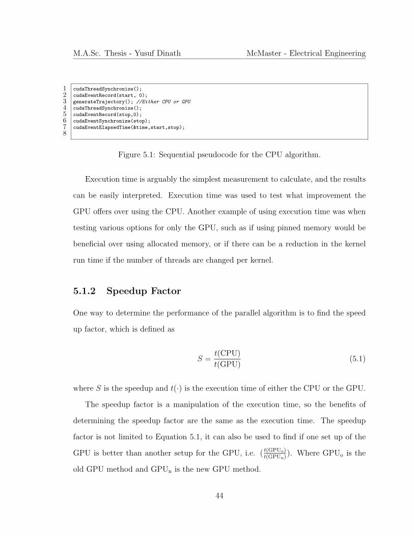
and will be accurately timed. Figure 5.1 shows the code to accurately time the CPU’s

and GPU’s execution time.

43


1 cudaThreadSynchronize();

2 cudaEventRecord(start, 0);

3 generateTrajectory(); //Either CPU or GPU

4 cudaThreadSynchronize();

5 cudaEventRecord(stop,0);

6 cudaEventSynchronize(stop);

7 cudaEventElapsedTime(&time,start,stop);

8

Figure 5.1: Sequential pseudocode for the CPU algorithm.

Execution time is arguably the simplest measurement to calculate, and the results

can be easily interpreted. Execution time was used to test what improvement the

GPU offers over using the CPU. Another example of using execution time was when

testing various options for only the GPU, such as if using pinned memory would be

beneficial over using allocated memory, or if there can be a reduction in the kernel

run time if the number of threads are changed per kernel.

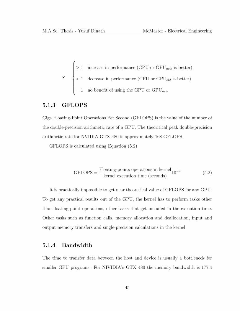
5.1.2 Speedup Factor

One way to determine the performance of the parallel algorithm is to find the speed

up factor, which is defined as

S =t(CPU)

t(GPU)(5.1)

where S is the speedup and t(·) is the execution time of either the CPU or the GPU.

The speedup factor is a manipulation of the execution time, so the benefits of

determining the speedup factor are the same as the execution time. The speedup

factor is not limited to Equation 5.1, it can also be used to find if one set up of the

GPU is better than another setup for the GPU, i.e. ( t(GPUo)t(GPUn)

). Where GPUo is the

old GPU method and GPUn is the new GPU method.

44


S

> 1 increase in performance (GPU or GPUnew is better)

< 1 decrease in performance (CPU or GPUold is better)

= 1 no benefit of using the GPU or GPUnew

5.1.3 GFLOPS

Giga Floating-Point Operations Per Second (GFLOPS) is the value of the number of

the double-precision arithmetic rate of a GPU. The theoritical peak double-precision

arithmetic rate for NVIDIA GTX 480 is approximately 168 GFLOPS.

GFLOPS is calculated using Equation (5.2)

GFLOPS =Floating-points operations in kernel

kernel execution time (seconds)10−9 (5.2)

It is practically impossible to get near theoretical value of GFLOPS for any GPU.

To get any practical results out of the GPU, the kernel has to perform tasks other

than floating-point operations, other tasks that get included in the execution time.

Other tasks such as function calls, memory allocation and deallocation, input and

output memory transfers and single-precision calculations in the kernel.

5.1.4 Bandwidth

The time to transfer data between the host and device is usually a bottleneck for

smaller GPU programs. For NIVIDIA’s GTX 480 the memory bandwidth is 177.4

45


GB/s. In both scenarios, only a relatively small amount of data is needed to generate

a significantly amount of data. Therefore, the time it takes to transfer memory to

the host from the device is much greater than the time is takes to transfer memory

to the device from the host.

5.2 Scenario 1

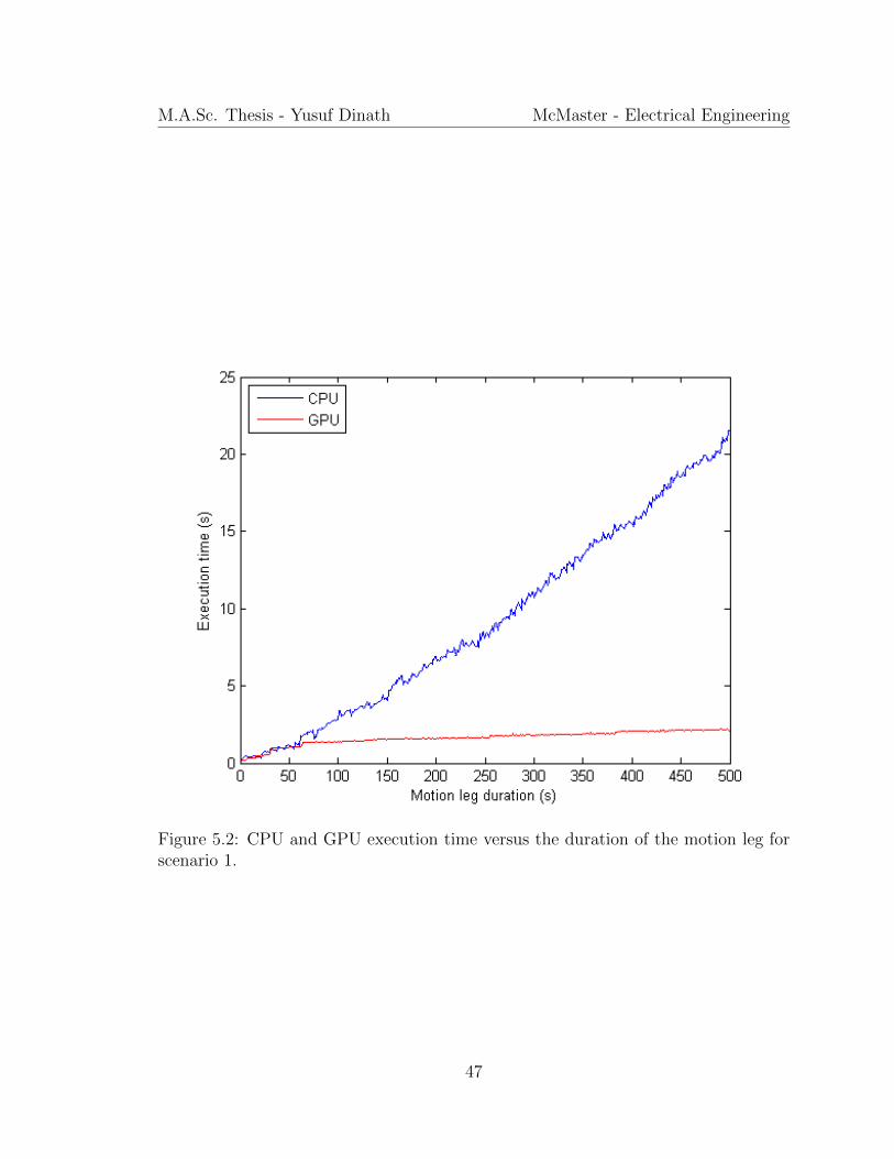
Figure 5.2 shows the CPU and GPU execution time versus the duration of the target’s

motion leg.

The CPU’s execution time had many fluctuation, however, there is a clear linear

increase in the CPU’s execution time. The CPU’s growth is as expected, with every

increment in the target’s motion leg duration the execution time should increase at

the same rate (slope is constant). Based on the CPU’s setup, the CPU’s execution

time will still increase steadily even if any of the for loops were switched in Figure

4.1.

For majority of the GPU’s execution time, it had a steady slope as time increased.

The GPU growth can be modelled with two functions, first growing similar to a f(x) =

√x function for durations approximately less than 60 seconds in this simulation, and

then increasing linearly approximately after durations of 60 seconds. There is a

significant amount of overhead added to the GPU’s exeuction time. However, as with

economies of scale, the cost of overhead reduces as the motion leg duration increases.

46


Figure 5.2: CPU and GPU execution time versus the duration of the motion leg forscenario 1.

47


Figure 5.3 demonstrates how as the target’s motion leg duration increases the

speedup factor also increases. However, there is a significant amount of fluctuation

when the duration of the target’s motion leg is small. Again, this is due to the

overhead costs associated with initializing the GPU.

At low motion leg durations, it is not clear if the GPU is better than the CPU.

However, as the duration of the motion leg increases beyond 60, it is clear the GPU

is beneficial.

Figure 5.3: Speedup factor of the GPU over the CPU vs the Duration of the MotionLeg for scenario 1.

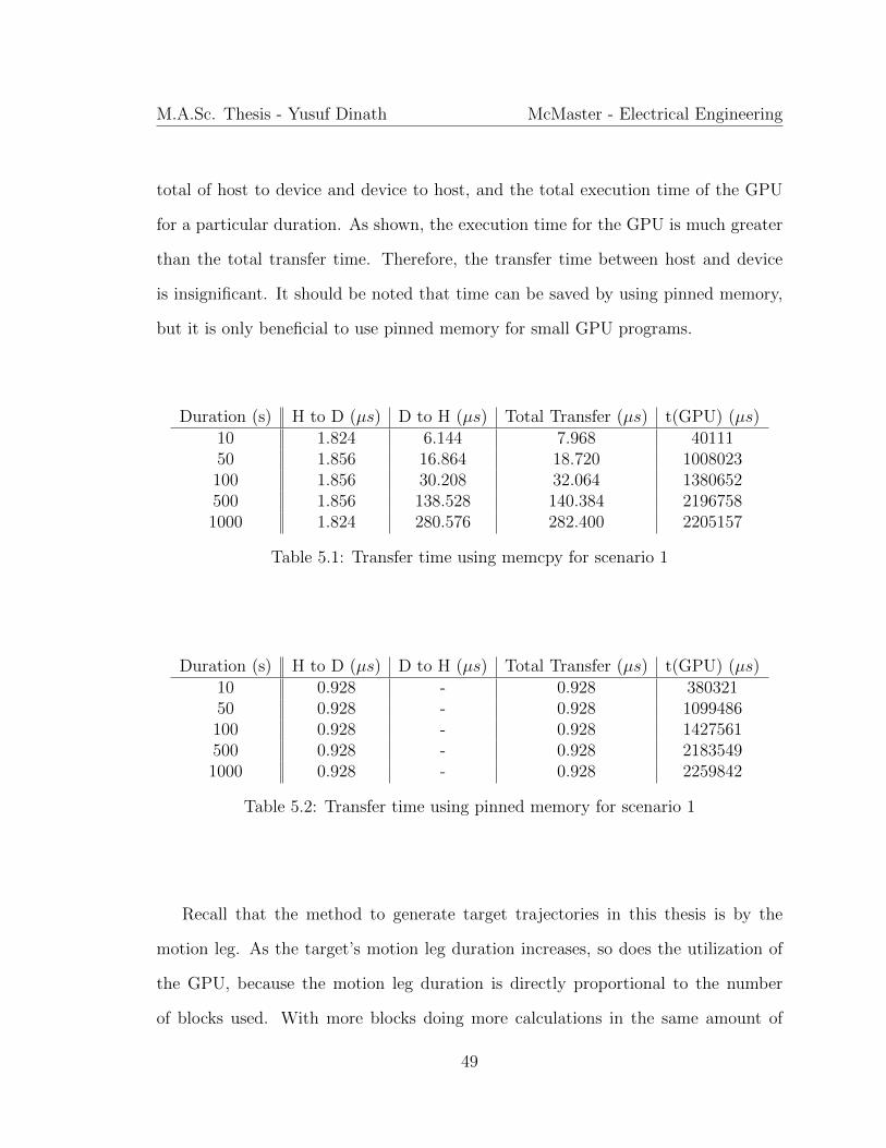
Tables 5.1 and 5.2 show the transfer time from host to device, device to host, the

48


total of host to device and device to host, and the total execution time of the GPU

for a particular duration. As shown, the execution time for the GPU is much greater

than the total transfer time. Therefore, the transfer time between host and device

is insignificant. It should be noted that time can be saved by using pinned memory,

but it is only beneficial to use pinned memory for small GPU programs.

Duration (s) H to D (µs) D to H (µs) Total Transfer (µs) t(GPU) (µs)10 1.824 6.144 7.968 4011150 1.856 16.864 18.720 1008023100 1.856 30.208 32.064 1380652500 1.856 138.528 140.384 21967581000 1.824 280.576 282.400 2205157

Table 5.1: Transfer time using memcpy for scenario 1

Duration (s) H to D (µs) D to H (µs) Total Transfer (µs) t(GPU) (µs)10 0.928 - 0.928 38032150 0.928 - 0.928 1099486100 0.928 - 0.928 1427561500 0.928 - 0.928 21835491000 0.928 - 0.928 2259842

Table 5.2: Transfer time using pinned memory for scenario 1

Recall that the method to generate target trajectories in this thesis is by the

motion leg. As the target’s motion leg duration increases, so does the utilization of

the GPU, because the motion leg duration is directly proportional to the number

of blocks used. With more blocks doing more calculations in the same amount of

49


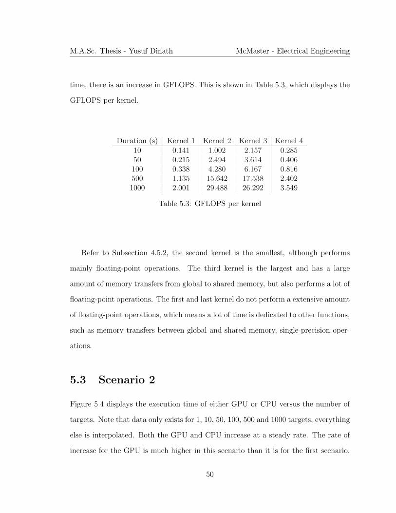
time, there is an increase in GFLOPS. This is shown in Table 5.3, which displays the

GFLOPS per kernel.

Duration (s) Kernel 1 Kernel 2 Kernel 3 Kernel 410 0.141 1.002 2.157 0.28550 0.215 2.494 3.614 0.406100 0.338 4.280 6.167 0.816500 1.135 15.642 17.538 2.4021000 2.001 29.488 26.292 3.549

Table 5.3: GFLOPS per kernel

Refer to Subsection 4.5.2, the second kernel is the smallest, although performs

mainly floating-point operations. The third kernel is the largest and has a large

amount of memory transfers from global to shared memory, but also performs a lot of

floating-point operations. The first and last kernel do not perform a extensive amount

of floating-point operations, which means a lot of time is dedicated to other functions,

such as memory transfers between global and shared memory, single-precision oper-

ations.

5.3 Scenario 2

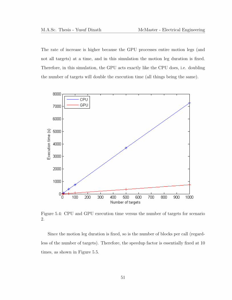
Figure 5.4 displays the execution time of either GPU or CPU versus the number of

targets. Note that data only exists for 1, 10, 50, 100, 500 and 1000 targets, everything

else is interpolated. Both the GPU and CPU increase at a steady rate. The rate of

increase for the GPU is much higher in this scenario than it is for the first scenario.

50


The rate of increase is higher because the GPU processes entire motion legs (and

not all targets) at a time, and in this simulation the motion leg duration is fixed.

Therefore, in this simulation, the GPU acts exactly like the CPU does, i.e. doubling

the number of targets will double the execution time (all things being the same).

Figure 5.4: CPU and GPU execution time versus the number of targets for scenario2.

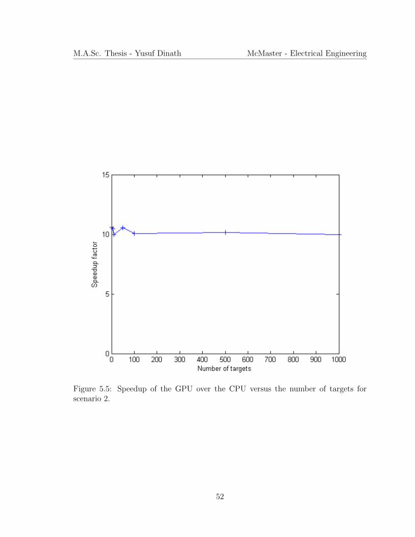
Since the motion leg duration is fixed, so is the number of blocks per call (regard-

less of the number of targets). Therefore, the speedup factor is essentially fixed at 10

times, as shown in Figure 5.5.

51


Figure 5.5: Speedup of the GPU over the CPU versus the number of targets forscenario 2.

52


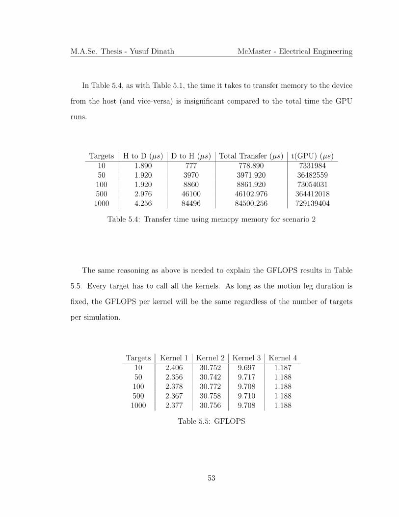
In Table 5.4, as with Table 5.1, the time it takes to transfer memory to the device

from the host (and vice-versa) is insignificant compared to the total time the GPU

runs.

Targets H to D (µs) D to H (µs) Total Transfer (µs) t(GPU) (µs)10 1.890 777 778.890 733198450 1.920 3970 3971.920 36482559100 1.920 8860 8861.920 73054031500 2.976 46100 46102.976 3644120181000 4.256 84496 84500.256 729139404

Table 5.4: Transfer time using memcpy memory for scenario 2

The same reasoning as above is needed to explain the GFLOPS results in Table

5.5. Every target has to call all the kernels. As long as the motion leg duration is

fixed, the GFLOPS per kernel will be the same regardless of the number of targets

per simulation.

Targets Kernel 1 Kernel 2 Kernel 3 Kernel 410 2.406 30.752 9.697 1.18750 2.356 30.742 9.717 1.188100 2.378 30.772 9.708 1.188500 2.367 30.758 9.710 1.1881000 2.377 30.756 9.708 1.188

Table 5.5: GFLOPS

53


5.4 Final Thoughts about Both Simulations

From profiling both applications, the majority of the time was spent in the third ker-

nel, which was expected. Generating random numbers took an insignificant amount

of time, especially when the duration of the motion leg was large. The number of

divergent branches was less than 1% of the total number of branches.

Often the branches diverged when storing and accessing memory location. There

are fewer locations than there are threads. Also, for the last block, when there is an

excess number of elements, the program needs to prevent accessing elements greater

than the duration.

54

Chapter 6

Conclusion and Future Work

This thesis demonstrates one approach to parallelize the generation of simulated tar-

get trajectories by using the GPU in conjunction with the CPU. The approach used

was to parallelize the entire motion leg of a target at a time. To begin, it was neces-

sary to define the problem. What is involved in generating target trajectories, both in

2D and in 3D, especially with the different coordinate systems. It was then necessary

to understand the programming environment. Programming in parallel has become

common because parallel hardware is cheaper. However, this does not mean that

parallel programming has become easier. The state equation needed to be manipu-

lated such that it could be used in developing a parallel algorithm; this required a

few assumptions about the motion models.

The results of parallelizing the motion legs were significant from the beginning.

However, there is room for improvement. The first way would be to reduce the

amount of overhead prior to calling the GPU. Other ways include taking advantage of

latest CUDA toolkits and newer generations of GPUs. Another option is to explore

parallelization of targets instead of motion leg’s time steps; having one target per

55


block and breaking up the motion legs into threads. To run one target per thread is

not advisable because of thread divergence.

Target generation is only the first step of many. User generated target trajectories

is necessary in testing algorithms such as the ones found in target tracking or path

detection. Having true data enables accurate comparisons between different trackers.

With target trackers and path detection algorithms, there is an increasing need for

large-scale target trajectories.

56

Bibliography

Bar-Shalom, Y. and Li, X. R. (1995). Multitarget-Multisensor Tracking: Principles

and Techniques. YBS Publishing, Storrs, CT.

EUROCONTROL and IfEN (1998). WGS 84 Implementation Manual. European

Organization for the Safety of Air Navigation, and Institute of Geodesy and Navi-

gation, Brussels, Belgium; and University FAF Munich, Germany, 2.1 edition.

Fung, J. and Mann, S. (2004). Computer vision signal processing on graphics pro-

cessing units. In IEEE International Conference on Acoustics, Speech, and Signal

Processing, volume 5, pages V93–V96.

Galben, G. (2011). New three-dimensional velocity motion model and composite

odometry-inertial motion model for local autonomous navigation. IEEE Transac-

tions on Vehicular Technology, 60(3), 771–781.

Harris, M. (2008). GPU Gems 3, chapter Chapter 39. Parallel Prefix Sum (Scan)

with CUDA. Addison-Wesley Professional, Upper Saddle River, NJ, 3 edition.

ICAO (2002). World Geodetic System - 1984 (WGS 84) Manual. International Civil

Aviation Organization, Montreal, Canada, 2 edition.

57


J.D. Owens, D. Luebke, N. G. M. H. J. K. A. L. T. P. (2005). A survey of general-

purpose computation on graphics hardware. In Eurographics 2005, State of the Art

Reports, pages 21–51.

J.P. Holdren, E. L. and Varmus, H. (2010). Report to the president and congress -

designing a digital future: Federally funded research and development in networking

and information technology. Technical report, Executive Office of the President and

President’s Council of Advisors on Science and Technology.

Kirk, D. B. and Hwu, W. W. (2010). Programming Massively Parallel Processors: A

Hands-on Approach. Morgan Kaufmann Publishers, Burlington, MA, 1 edition.

Li, X. R. and Jilkov, V. P. (2003). Survey of maneuvering target tracking. part 1:

Dynamic models. IEEE Transactions on Aerospace and Electronic Systems, 39(4),

1333–1364.

NIVIDA (2012). Cuda toolkit. http://developer.nvidia.com/cuda-toolkit.

NVIDIA (2011). CUDA C Programming Guide. NVIDIA, Santa Clara, CA, 4.2

edition.

NVIDIA (2012). CUDA C Best Practices Guide. NVIDIA, Santa Clara, CA, 4.1

edition.

Sanders, J. and Kandrot, E. (2011). CUDA by Example: An Introduction to General-

Purpose GPU Programming. Addison-Wesley Professional, Upper Saddle River,

NJ, 1 edition.

Sankowski, M. (2011). Reference model of aircraft movements in geodetic coordinates.

In Radar Symposium (IRS), 2011 Proceedings International, pages 874–879.

58


T. Kirubarajan, Y. Bar-Shalom, K. P. and Kadar, I. (2000). Ground target tracking

with topography-based variable structure imm estimator. IEEE Transactions on

Aerospace and Electronic Systems, 36, 26–46.

T. Kirubarajan, Y. Bar-Shalom, K. P. I. K. B. A. E. E. (1998). Tracking ground tar-

gets with road constraints using an imm estimator. In IEEE Aerospace Conference,

volume 5, pages 5–12.

Tewari, A. (2007). Atmospheric and Space Flight Dynamics: Modeling and Simulation

with MATLAB R© and Simulink R© (Modeling and Simulation in Science, Engineering

and Technology). Birkhauser Boston, Cambridge, MA, 1 edition.

59

Large-Scale Motion Modelling using a Graphical Processing Unit

Documents

Transcript of Large-Scale Motion Modelling using a Graphical Processing Unit