Large Scale Mobile Visual Search

Shih-Fu ChangJune 2012

(by Mac Funamizu)Ricoh, HotPaper

2

70,000 TB/year, 100 million hours

60 hours of video uploaded every minute

broadcast

Social portals

video blogs

• Many domains broadcast, entertainment, social media

• 1 month YouTube > 60 years video of 3 major TV networks

The Explosive Growth of Visual Data

2

4 billion video views  per day in 2012

(Slide from Lexing Xie)

1994

Many research & commercial search engines

19951996199719981999200020012002200320042005200620072008200920102011VideoGoogle

digital video | multimedia lab

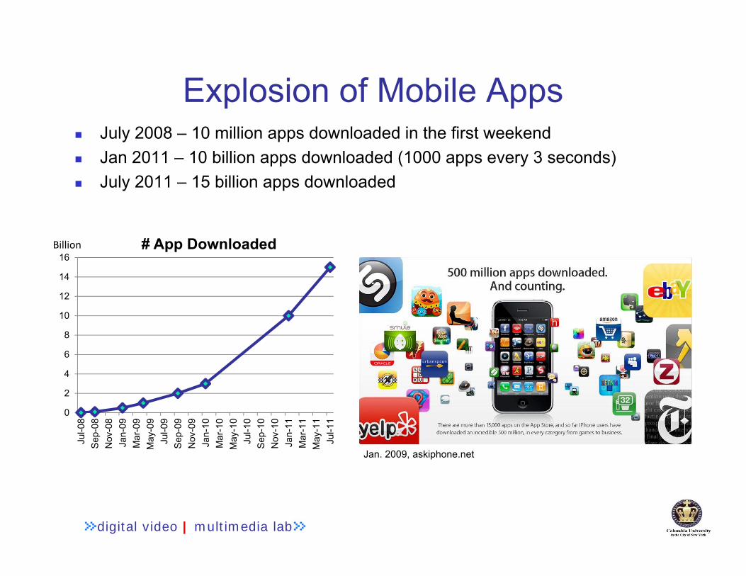
Explosion of Mobile Apps July 2008 – 10 million apps downloaded in the first weekend Jan 2011 – 10 billion apps downloaded (1000 apps every 3 seconds) July 2011 – 15 billion apps downloaded

0

2

4

6

8

10

12

14

16

Jul-0

8S

ep-0

8N

ov-0

8Ja

n-09

Mar

-09

May

-09

Jul-0

9S

ep-0

9N

ov-0

9Ja

n-10

Mar

-10

May

-10

Jul-1

0S

ep-1

0N

ov-1

0Ja

n-11

Mar

-11

May

-11

Jul-1

1

# App Downloaded

Jan. 2009, askiphone.net

Billion

digital video | multimedia lab

Mobile meets Visual Search

Expanded visual sense

Expanded audio sense

Expanded food sense

How does Mobile Visual Search work?

Image Database

1. Take a picture

0 20 40 60 80 100 120 1400

0.1

0.2

0.3

0.4

0.5

2. Send image or features

3. Send via mobile networks

4. Visual search on server database

0 20 40 60 80 100 120 1400

0.1

0.2

0.3

0.4

0.5

0 20 40 60 80 100 120 1400

0.1

0.2

0.3

0.4

0.5

0 20 40 60 80 100 120 1400

0.1

0.2

0.3

0.4

0.5

5. Send results back

Challenges for MVS

Image Database

1. Take a picture

0 20 40 60 80 100 120 1400

0.1

0.2

0.3

0.4

0.5

2. Image feature extraction

3. Send via mobile networks

4. Visual matching with database images

0 20 40 60 80 100 120 1400

0.1

0.2

0.3

0.4

0.5

0 20 40 60 80 100 120 1400

0.1

0.2

0.3

0.4

0.5

0 20 40 60 80 100 120 1400

0.1

0.2

0.3

0.4

0.5

5. Send results backLimited power/memory/

speed

Limited bandwidth

Gigantic Database

But need fast response 

(<  1‐2 seconds)

MVS calls for Distributed Optimization

Client: fast feature extraction

Radio : transmit compact codes

Server: scalable indexing over millions/billions

Case Study (MVS, Girod et al, 2011)

Mobile Search System by Hashing

9

Light ComputingCompact Hash

Code Big Data Indexing

He, Feng, Liu, Cheng, Lin, Chung, Chang. Mobile Product Search with Bag of Hash Bits and Boundary Reranking, CVPR 2012.

Server:• 1 million product images crawled from Amazon, eBay and Zappos

• Hundreds of categories; shoes, clothes, electrical devices, groceries, kitchen supplies, movies, etc. 

Speed• Feature extraction: ~1s • Transmission: 80 bits/feature, 1KB/image

• Serer Search: ~0.4s• Download/display: 1‐2s

Columbia MPS System: Bags of Hash Bits and Boundary features

video demo

Brief Review of Image Features

• Characterize visual content by local features (keypoints): – Interesting content– Precise localization– Repeatable detection under variations of scale, rotation, etc

(Slide of K. Grauman)11

Example: keypoint detection

Original image41

2

Sampling withstep  =2

• Compute image Gaussian scale pyramid• Keypoints from local maxima in scale space• Many solutions: SIFT, SURF, MSER, BRIEF

(Slide of K. Grauman)

12

SIFT: Histogram of oriented gradients over local grids• rotation invariant by orientation alignment• scale invariant by scale space detection

Describe Appearance of Local Features[Lowe, ICCV 1999]

S.-F. Chang, Columbia U. 13

Compute gradient in a local patch

14K. Grauman, B. Leibe

Matching with Local Features• local features facilitate robust matching over geometric and

photometric transformations

Local Features, e.g. SIFT

Slide: David Lowe

Example

Initial matches

Spatial consistency required

Slide : J. Sivic

Estimate the Complexity

• 500 local features per image– file size ~128 Kbytes– more than 10 seconds for transmission over 3G

• Database indexing– 10 millions images need 5 billions local features– Finding matched features becomes challenging

• Idea: directly compute compact index codes on mobile devices

Standard Approach: Tree‐Based Indexing

• O(log n) search time (20 bits for 1 million nodes)• But “curse of high dimensionality” problem• Hard to store on mobile devices

17

treeKD‐tree

A Different Approach: hashing• Each local feature coded as hash bits

– locality sensitive, efficient for high dimensions

• Each image is represented as Bag of Hash Bits

011001100100111100…

110110011001100110…

18

Locality‐Sensitive Hashing

• Sublinear search time                  for ε‐approximate NN search. 

0

1

0

10

1

Feature Vector

19

hash function

random

101 Query

[Gionis,  Indyk, and Motwani 1999] [Datar et al. 2004]

D(q, x) (1)D(q, xnn )x is an ε‐approximate NN if 

Efficient Search by Hash Table

20

• O(1) search time with short bits (<=50) and a single table.• Both time and storage efficient.

xi

n

q01101

01101

01110

01111

01100

hash tablehash bucket address

Hashing: Active Research Topic• Several categories published in KDD, ICML, CVPR, ICDM

21

Unsupervised Hashing

LSH, PCAH, ITQ,KLSH, SH, AGH

Semi‐Supervised Hashing

SSH, WeaklySH

Supervised Hashing

RBM, BRE, MLH, LDAH

• Principle – explore data distributions– Similar hash codes for similar points (accuracy)– Balanced and non‐redundant hash bits (time)

Search accuracy

Unsupervised hash

2

, 1( ) || ||

N

pq p qp q

D Y W Y Y

Balanced bucket size

1

1

min ( , ..., , ..., )

while ( ) 0

k MN

pp

I y y y

E y Y

SPICA Hash, He et al, CVPR 11

• SPICA Hash: jointly optimize search accuracy & time

Learning Based Hashing vs. Random Hashing

Bucket indexBu

cket size LSH

SPICA Hash

Reduce candidate set from 1Million to 10K @ 50% recall

Random LSH often leads to unbalanced codes

If there is supervised informationSemantic Supervision

24CVPR 2012

Metric Supervision

similar

dissimilardissimilar

similar

dissimilar

Design Hash Codes to Match Supervised Information

25

similar

dissimilar

01

Preferred hashing

Use Code Inner Products to Match Supervised Labels

26

S

x2

x3

x1 similar

supervised hashing

labeled data

1 -1 11 -1 1-1 1 -1

1 1 1-1 -1 11 1 -1

ХTcode matrix

1 1 -11 1 -1-1 -1 1

x1

x2

x3

x1 x2 x3

pair-wise label matrix

code inner products

rx1

x2

x3

code matrix

fitting

Liu, Wang, Ji, Jiang, Chang, CVPR2012

Learning Supervised Hash

• Easy to optimize and extend to kernels• Sequential learning

27

sample

hash bitHashing: 

Design hash codes to match supervised information

1 Million Tiny Images

28

Torralba and Fergus, TPAMI 2008

• Search 1 million images from Web

• 2000 random images as queries

• Top 5000 nearest samples as consistent pairs

Supervised kernel hashing

Spherical Hashing• linear projection ‐> spherical partitioning

• Asymmetrical hash bits: tighter regions for +1• Learning: find optimal spheres in the space

29

Heo, Lee, He, Chang, Yoon, CVPR 2012

Spherical Hashing Performance• 1 Million Images: GIST 384‐D features

30

Point‐to‐Point Search vs. Point‐to‐Hyperplane Search

point query

nearest neighbor

hyperplanequery

nearest neighbor

normalvector

31

Hashing Principle: Point‐to‐Hyperplane Angle

32

The ideal neighbors ┴ w

Bilinear Hashing

• bilinear hash bit: +1 for || points, ‐1 for ┴ points

Bilinear‐Hyperplane Hash (BH‐Hash) 

33

query normal w or database point x 2 random projection vectors

Liu, Jun, Kumar, Chang, ICML12

A Single Bit of Bilinear Hash

34

u v1

1

‐1 ‐1

x1

x2

// bin┴ bin

Theoretical Collision Probability

35

highest collision probability for active hashing so far

Double the collision prob

Jain et al. ICML 2010

Active SVM Learning with Hyperplane Hashing

• Linear SVM Active Learning over 1 million data points

CVPR 2012 36

• How difficult is approximate nearest neighbor search in a dataset?

Understand Difficulty of Approximate Nearest Neighbor Search

Toy example

q

D(q, x) (1)D(q, xnn )x is an ε-approximate NN if

Search not meaningful!

A concrete measure of difficulty of search in a dataset?

He, Kumar, Chang, ICML 2012

• A naïve search approach: Randomly pick a point and return that to be the NN

Relative Contrast

qCr Drandom

Dnn

Relative Contrast

E x[D(q, x)]

D(q, xnn )

Cr Eq, x[D(q, x)]Eq[D(q, xnn )]

• High Relative Contrast easier search• If , search not meaningfulCr 1

He, Kumar, Chang, ICML 2012

• With CLT, and binomial approximation

Estimation of Relative Contrast

ϕ - standard Gaussian cdf

Cr Drandom

Dnn

1[11((1/ ')1/ n) ']1/p

n

p =1

σ' – a function of data properties e.g., dimensionality and sparsity

d ' 0 Cr 1

• Data sampled randomly from U[0,1]

Synthetic Datare

lativ

e co

ntra

st

rela

tive

cont

rast

higher dimensionality  bad sparser vectors  good

• Data sampled randomly from U[0,1]

Synthetic Datare

lativ

e co

ntra

st

rela

tive

cont

rast

lower p  good Larger database  good

Predict Hashing Performance of Real‐World Data

16 bits

Dataset Dimensionality (d)

Sparsity(s)

Relative Contrast (Cr) for p = 1

SIFT 128 0.89 4.78

Gist 384 1.00 1.83

Color Hist 1382 0.027 3.19

Imagenet BoW 10000 0.024 1.90

28 bits

Multi‐Table Hashing• Larger table increases precision but degrades recall• Common trick: multi‐table hashing

• Union of multi‐table results increases precision and keeps recall

• But the number of hash bits 2X: bad for mobile

43

matched bucket in k‐bits table

matched bucket in k+1 bits Table II

matched bucket in k+1 bits Table

Bit Reuse for Multi‐Table Hashing• To reduce transmission size

– Reuse top optimal hash bits by random sampling

44

1 0 0 1 1 1 0 0 0 0 1 0 1 0 1 0 . . . 0 0 1 1 0 1 1 1

Optimal hash bit pool (e.g., 80 bits, PCA Hash or SPICA hash)

Random subset

Random subset

Random subset

Random subset. . .

Table 1 Table 2 Table 11 Table 12. . . 32 bits

Union Results

Data Sets• Data set 1: 400K products crawled from ebay, zappos;

– more than 100 diverse categories – 205 queries, each has one GT in database

• Data set 2: 300K product images crawled from amazon – 20 categories, mainly shoes, home supplies– 135 queries, each has one GT in database

• On average, 100-200 local features(LF) for each image

Example queries and groundtruths for data set 145

He, Feng, Liu, Cheng, Lin, Chung, Chang. Mobile Product Search with Bag of Hash Bits and Boundary Reranking, CVPR 2012.

Performance• CHoG approach [V. Chandrasekhar et al 2009]: Compress local features with CHoG on mobile + BoWwith VocTree (1M codewords) on server

30% higher recall and 6X‐30X search speedup

46

Rerank Results with Boundary Features• Use automatic salient object segmentation for every image in DB [Cheng et al, CVPR 2011]

• Compute boundary features: normalized central distance, Fourier magnitude

• Invariance: translation, scaling, rotation

47

Boundary Feature – Central Distance

Distance to Center D(n) FFT: F(n) 48

Reranking with boundary feature

49

Server:• 400,000  product images crawled from Amazon, eBay and Zappos

• Hundreds of categories; shoes, clothes, electrical devices, groceries, kitchen supplies, movies, etc. 

Speed• Feature extraction: ~1s • Transmission: 80 bits/feature, 1KB/im• Serer Search: ~0.4s• Download/display: 1‐2s

Columbia MPS System: Bags of Hash Bits and Boundary features

video demo

He, Feng, Liu, Cheng, Lin, Chung, Chang. Mobile Product Search with Bag of Hash Bits and Boundary Reranking, CVPR 2012.

How to guide the user to take a successful mobile query?– Which view will be the best query?

• For example, in mobile location search:

• Or in mobile product search:

51

Multi-View Challenge

Mobile Location Search

• 300,000 images of 50,000 locations in Manhattan• Collected by the NAVTEQ street view imaging system

Geographical distribution52

• Location Sampling– Locations are imaged at a four-meter interval on average– Six camera views for each location separated by 45⁰

• Visual Data Organization– Six views (images)– Also provide panorama (used for visualization in this work) 1

2

34

5

6

NAVTEQ 0.3M NYC Data Set

53Images  from Navteq

digital video | multimedia lab

More Challenges on Mobile Clients

Image quality variations Exposure Shadow Distance Obstruction Blur Weather Day/Night

Navteq NYC Data

Not every view is equally good for search

Subsample 200 locations to “# of searchable views” using cropped Google street view

# of searchable 

views

1

234

6

5

0

• Recognition accuracy far from perfect– Less than 50% visual location searches successfulinitial tests [Columbia Visual Location Search, ‘11]

Solution: Active Query Sensing Guide User to a More Successful Search Angle

Active Query Sensing [Yu, Ji, Zhang, and Chang, ACMMM, 2011]

Video demoMobile App Demo

• Offline– Salient view learning for each reference location

• Online– Viewing angle prediction of the first query– Suggest new views by majority voting

Active Query Sensing System

57

Location2

Location N

1 2 3 4 5 6

…

Location3

Location4

1 2 3 4 5 6

1

2

3 4 5 6

1 2

3

4 5 6

1

2

34

5

6Query view

For each location, we have its most salient

view

The majority of the salient views decides the

suggested (second) query

3

3 4

2

Location1

58Salient view

View 6

View 5

View 4

View 3

View 2

View 1

Active Query Sensing (case 1)known query view

What if query view is unknown?• Step I: Predict the view angle of the first query

Offline Training: Train view prediction classifiers offline

Online Prediction: View alignment based on the image matching

Our solution is to combine them both

59

Query

Active Query Sensing (case 2)unknown query view

Location2

Location N

1 2 3 4 5 6

…

Location3

Location4

1 3 4 5 6

1

2

3 4 5 6

1 2

3

5 63 4

2

Viewing AnglePrediction

Salient View (Offline)

View Change3

4

2

Turn 90 degrees to the right

60

• Step II: Majority voting in terms of view change

User Interface• Help user determine whether the first query is correct

– Panorama– Geographical map context

• Guide the user to take the second query– Compass, camera icon

• Show point of interest

61

AQS Examples

62

First Query First Result Ask AQS Taking Second Query Second Result

Performance Improvement

• The AQS system helps user select the best angle for searching location

• It reduces failure rate by more than half

Failure rates over successive query iterations.

• Overall Performance

63

Reduce error rate from 28% to 12%

Conclusions• Bags of Hash Bits (BoHB) for fast mobile product search– Simultaneously address power, bandwidth, and large database issues

• Promising research in hashing• Active Query Sensing for interactive search

– New paradigm for interactive mobile visual search– Guide user in the loop

64

References• (Hash Based Mobile Product Search)

J. He, T. Lin, J. Feng, X. Liu, S.‐F. Chang, Mobile Product Search with Bag of Hash Bits and Boundary Reranking, CVPR 2012

• (SPICA Hash)J. He, R. Radhakrishnan, S.‐F. Chang, C. Bauer, Compact Hashing with Joint Optimization of Search Accuracy and Time, CVPR 2011 (oral).

• (Supervised Kernel Hash)W. Liu, J. Wang, R. Ji, Y. Jiang, and S.‐F. Chang, Supervised Hashing with Kernels, CVPR 2012 (oral)

• (Spherical Hashing)Jae‐Pil Heo, YoungWoon Lee, Junfeng He, Shih‐Fu Chang, Sung‐eui Yoon. Spherical Hashing. CVPR 2012.

• (Hyperplane Hashing)Wei Liu, Jun Wang, Yadong Mu, Sanjiv Kumar, Shih‐Fu Chang. Compact Hyperplane Hashing with Bilinear Functions. ICML 2012

• (Active Mobile Location Search)F. X. Yu, R. Ji, T. Zhang, S.‐F. Chang. Active Query Sensing for Mobile Location Search, ACM Multimedia 2011.

65