Large-Network Travel Time Distribution Estimation for

Ambulances

Bradford S. Westgate∗, Dawn B. Woodard, David S. Matteson,

Shane G. Henderson

December 27, 2015

Abstract

We propose a regression approach for estimating the distribution of ambulance travel times

between any two locations in a road network. Our method uses ambulance location data that

can be sparse in both time and network coverage, such as Global Positioning System data.

Estimates depend on the path traveled and on explanatory variables such as the time of day

and day of week. By modeling at the trip level, we account for dependence between travel

times on individual road segments. Our method is parsimonious and computationally tractable

for large road networks. We apply our method to estimate ambulance travel time distribu-

tions in Toronto, providing improved estimates compared to a recently published method and

a commercial software package. We also demonstrate our method’s impact on ambulance fleet

management decisions, showing substantial differences between our method and the recently

published method in the predicted probability that an ambulance arrives within a time thresh-

old.

Keywords: Transportation; Traffic; OR in health services; Travel time estimation; Markov

Chain Monte Carlo.

∗Corresponding author. Email: westgatebs@alma.edu. Phone: 603-321-3295. 253 Swanson Academic Center, Alma

College, 614 W. Superior St., Alma, Michigan 48801.

1

1 Introduction

Estimates of ambulance travel times on arbitrary routes in a road network are used in ambulance

dispatch decisions, base location algorithms, and real-time redeployment methods [4, 7, 13, 23,

32]. In many of these applications it is important to capture the uncertainty in the travel

time, by predicting the entire travel time distribution rather than just the expected travel time

[16, 39]. For instance, taking into account uncertainty in the travel time of ambulances to

the scene of an emergency can substantially increase the survival rate of cardiac patients, by

improving fleet management decisions and thus reducing response times [9, 25]. Also, ambulance

fleet performance is measured by the fraction of emergency calls for which the response time is

less than a specified threshold, and forecasting this performance measure requires travel time

distribution information [22]. Travel time distributions are also used in applications for other

vehicle fleets, including calculation of driving directions for private vehicles using taxi data [38],

allocation of railcars [35], and routing and scheduling of courier vehicles [26].

We propose a regression approach for estimating the distribution of an ambulance travel

time on an arbitrary route in a road network. The prediction depends on the route and on

explanatory variables such as the time of day and day of week. Our method uses information

from historical trips on the network, specifically the total travel time and estimated route for

each trip. In order to predict the travel time distribution for a particular route, we do not

require historical trips that take precisely the same route. Instead, our statistical approach

uses information from all the historical trips by learning shared properties like the effects of

time of day and types of road traversed. The model we use is intuitive and its parameters are

interpretable. Our method is computationally efficient, scaling effectively to large road networks

and large historical trip databases.

Two features of ambulance travel times motivate our modeling choices. First, ambulances

traveling at lights-and-sirens speeds are less affected by traffic than other vehicles [1, 20, 37].

Therefore, historical ambulance trips are the most relevant source of information for travel times,

and real-time traffic flow information from other vehicles is less useful. Second, ambulance

trips are comparatively rare, implying that ambulance data is sparse in time and road network

coverage. Roads that are not major thoroughfares may have only a few ambulance trips on

them per year.

To estimate the route taken in the historical trips, we use Global Positioning System (GPS)

measurements taken during travel. This source of data is called floating car data or automatic

2

vehicle location data, and is increasingly available for many types of vehicles, including ambu-

lances, taxis, and personal vehicles, via GPS-enabled smartphones or 2-way navigation devices

(e.g. Garmin or TomTom) [14]. Unlike other sources of travel time data, it does not require

instrumentation on the roadway, and thus is the only source of data available to estimate travel

times that has the prospect of comprehensive network coverage.

Despite the rise in availability of floating car data, there are still few methods available to

utilize floating car data for travel time distribution prediction. Hofleitner, Herring, and Bayen

[15] and Hofleitner, Herring, Abbeel, and Bayen [14] take a traffic flow perspective, modeling at

the level of the network link (a road segment between two intersections). They use a dynamic

Bayesian network for the unobserved traffic conditions on links and model the link travel time

distributions conditional on the traffic state. Their method is applied to a subset of the San

Francisco road network with roughly 800 links, predicting travel times using taxi fleet data and

validating with additional data sources.

In previous work, we introduced a Bayesian model for simultaneous travel time distribution

and path estimation for a set of vehicle trips [37]. Like Hofleitner et al., we modeled travel times

at the link level. Our method was applied to estimate ambulance travel times on a subregion of

Toronto.

In an early paper, Erkut et al. [8] estimate ambulance and fire truck speeds in St. Albert,

AB, Canada, as part of a study to select new locations for a fire station and ambulance base.

They use three road classes (freeway, main roads, and residential roads), and also account for

time-of-day and season by estimating different speeds for rush hour and non-rush hour and for

summer and winter. They estimate average speeds using historical data, interviews with drivers,

and road tests. They do not consider the distribution of travel times.

Jenelius and Koutsopoulos [17] propose a framework for estimating the distribution of travel

times while incorporating weather, speed limit, and other explanatory factors. They point

out that previous approaches such as Hofleitner et al. and Westgate et al. [14, 15, 37] assume

that the link travel times are independent within a vehicle trip, perhaps conditional on the

traffic state. This contrasts with empirical evidence suggesting that the link travel times are

strongly correlated, even after conditioning on time of day and other explanatory factors [3, 29].

Therefore, they capture correlation using a moving average specification for the link travel times.

Their framework is applied to estimate travel times for a particular route in Stockholm.

In contrast to these approaches, we model travel times at the trip level instead of the link

level. This naturally incorporates dependence between link travel times. The ambulance route

3

is taken into account in the specification of the trip travel time parameters, such as the median

travel time. This trip-level approach is related to the regression approach of Budge, Ingolfsson,

and Zerom [6], who model the travel time distribution for an ambulance trip as a function of

shortest-path distance between the start and end locations. They assume that the log travel time

follows a t-distribution, where the centering and scale parameters are either a nonparametric or

parametric function of the shortest-path distance. These functional forms enable their method

to be flexible but still interpretable. Like them we take a regression approach, but we also

incorporate dependence on the route taken, time of day, and other explanatory factors, justifying

our modeling choices empirically. This captures the fact that locations near primary roads can

be reached more quickly than other locations, for example. A downside of modeling at the trip

level is that travel time predictions cannot be updated to reflect changing conditions while a

vehicle is enroute. However, this is not a drawback in the ambulance setting, because travel

time estimates are used for ambulance dispatch decisions and base placement, rather than for

route selection.

We use our method to predict ambulance travel times for the entire road network of Toronto.

The size of the road network (68,272 links) is an order of magnitude larger than in previous

applications of travel time distribution estimation based on floating car data [6, 14, 15, 17, 37],

and the number of historical vehicle trips (157,283) is also larger than these previous applications.

We compare the prediction accuracy of our method to that of Budge et al. [6], Westgate et al.

[37], and a commercial software package for mean travel time estimation. We also consider the

effect of various simplifications of our model, and investigate the accuracy of our model when

the time effect on travel times is artificially inflated.

Finally, we evaluate the effect of using our method for ambulance fleet management, relative

to that of Budge et al. [6]. We select a set of representative ambulance posts in Toronto, and

calculate which ambulance post is estimated to be the closest in median travel time to each

intersection in Toronto. Many intersections have different estimated closest posts, according to

the two methods, so the two methods would recommend that a different ambulance respond to

emergencies at these locations, if the closest ambulance is dispatched. Next, we calculate the

probability that an ambulance is able to respond on time (within a specified time threshold)

from the closest post to each intersection of the city. We find substantial differences in these

probabilities between the two methods. These appear to arise because our method captures

differences in speeds between different types of roads, unlike the method of Budge et al.

Commercially available vehicle travel time estimates typically consist of estimated expected

4

travel times rather than distribution estimates, so they cannot be used to calculate the prob-

ability an ambulance arrives within a time threshold, or for ambulance deployment algorithms

where simulated travel times are needed. Also, these estimates are calculated for standard ve-

hicle speeds, not lights-and-sirens ambulance speeds. However, they are still useful for point

estimation performance comparisons, as long as they are corrected for bias. Specifically, we in-

vestigate travel time estimates from TomTom, a maker of navigation devices. Bias adjustment

does not fully account for the differences between the TomTom context and ours, so our results

should not be interpreted as an evaluation of the quality of TomToms estimates.

The article is organized as follows. In Section 2, we introduce the data from Toronto and

highlight the exploratory data analysis that motivates our modeling choices. In Section 3,

we introduce our statistical model and estimation method. In Section 4, we give results and

compare to the alternative methods. We draw conclusions in Section 5. In Appendices A, B,

and C, we give details on data preprocessing, fastest path estimation, and our implementation

of the method of Budge et al.

2 Toronto EMS Data

We use our method for a study of ambulance travel times in Toronto, Ontario. The goal is

to estimate the distribution of time required for an ambulance to drive to the scene of a high-

priority emergency, in which case the ambulance uses lights and sirens, and travels at high

speed. The data are provided by Toronto EMS (Emergency Medical Services), and include all

such ambulance trips in Toronto during the years 2007 and 2008. We analyzed a subset of these

data from the Leaside region of Toronto in previous work [37]; here we estimate travel times on

the entire Toronto road network, which consists of 68,272 links.

The data associated with each trip include the approximate start and end times and locations

of the trip, as well as sparse GPS location and speed readings during the trip. The GPS

measurements are stored every 200 meters (m) of travel or 240 seconds (s), whichever comes

first (typically the distance constraint is satisfied first for lights-and-sirens travel).

Cleaning and preprocessing the data is a challenge, due to factors such as human error in

recording the start and end times and locations of the trips, the presence of trips where the

ambulance doubled back on itself, and the presence of GPS measurement error. These challenges

and our preprocessing algorithm are described in Appendix A. After preprocessing we are left

with 157,283 ambulance trips, having removed 20,443 trips. The median shortest-path distance

5

between the start and end locations is 2,530 m.

To apply our method, we first estimate the path traveled for each ambulance trip, using the

GPS data. Many such “map-matching” methods could be used [21, 22, 27, 28]; we use the one

introduced in [36].

2.1 Exploratory Analysis

Here we highlight exploratory analysis of the Toronto EMS data, after trip preprocessing. Re-

sults from this analysis motivate the modeling assumptions described in Section 3.1. After

preprocessing, each trip consists of a sequence of GPS readings. To assist exploratory analy-

sis of the travel time distribution between any two locations, we map the first and last GPS

readings of each trip to the nearest intersections in the network, to use as estimated start/end

locations (this differs from our travel time model, in which trips are allowed to start and end in

the interior of links). We collect the most common pairs of start/end intersections for the trips

in the dataset; there are 10 start/end pairs with at least 40 trips between them.

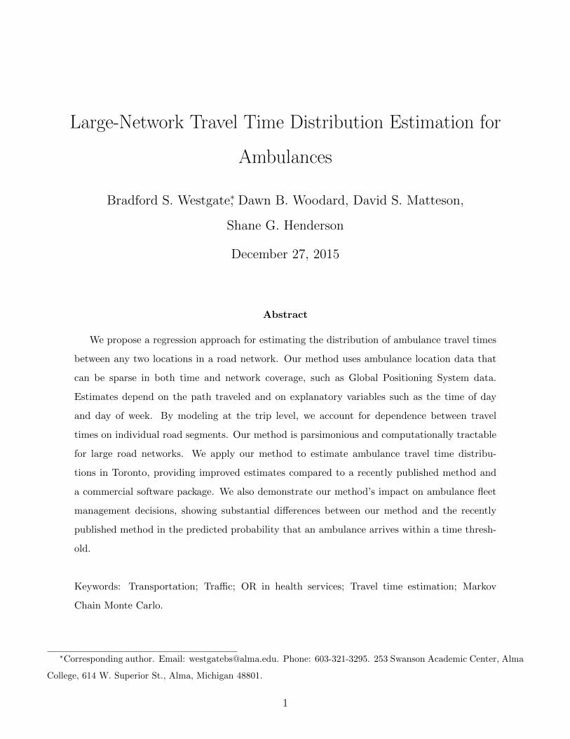
Figure 1 shows normal Quantile-Quantile (Q-Q) plots for the log travel times between the

four most common start/end pairs in the dataset. The shortest-path distance between the

start and end locations is shown above each Q-Q plot. Also shown on the Q-Q plots are 95%

pointwise confidence bands, under the null hypothesis that the log travel times are normally

distributed. Only 6% of the observed travel times in the four plots fall outside the pointwise

confidence bands, which suggests that the lognormal assumption is reasonable (if it is correct

then we expect roughly 5% of the observations to fall outside of the bands). Although nearly

all of the points outside the confidence bands occur on a single one of these four plots, this is

not surprising because the points on a Q-Q plot are strongly dependent. Similar Q-Q plots have

been constructed for the next most common start/end pairs, and they also suggest lognormal

travel times.

The lognormal distribution has been observed in practice and also used as a model for both

link and trip travel times repeatedly in the literature [1, 2, 18, 24]. We use the lognormal

distribution because it is supported by exploratory data analysis, and also to provide a parsi-

monious parametric model. Due to the sparseness in data, there are typically few trips between

any two locations in the road network. While Budge et al. found that ambulance travel times

were heavier-tailed than the lognormal (they used log-t distributions), they did not condition

on the start and end locations of the trips. For the Toronto ambulance data, if one does not

6

● ● ● ●●●

●●●●●●

●●●●●●●

●●●●●●

●●●●●●●●●

●●●●●●●●●

●●●●

●●●●●●●●●●

●● ●

●

−2 −1 0 1 2

4.8

5.0

5.2

5.4

Trip distance: 1868 m

Normal Quantiles

Log

Trip

Tra

vel T

imes

●

● ●

●●

●●●●●●●●●

●●●●●●●●●

●●●●●●●

●●●●●●●

●●●●

●●●●●

●●● ●

●●

−2 −1 0 1 2

4.6

4.8

5.0

5.2

5.4

5.6

Trip distance: 1691 m

Normal Quantiles

Log

Trip

Tra

vel T

imes

●

●●

●●●●●●●●●●●●●●●●●●●

●●●●●●●

●●●●

●●●●

●●●●

●●●

●●●● ●

●

●

−2 −1 0 1 2

4.6

4.8

5.0

5.2

Trip distance: 1606 m

Normal Quantiles

Log

Trip

Tra

vel T

imes

●● ● ●

●

●●●●

●●●●●●●●●●

●●●●●●●●

●●●●●

●●●●

●●●●

●●●●●●

●●

● ●

−2 −1 0 1 2

4.2

4.6

5.0

5.4

Trip distance: 1180 m

Normal Quantiles

Log

Trip

Tra

vel T

imes

Figure 1: Normal Quantile-Quantile plots for travel times between the four most common start/end

location pairs in the Toronto EMS dataset.

condition on the start and end locations, the travel time distribution also has heavier tails than

the lognormal.

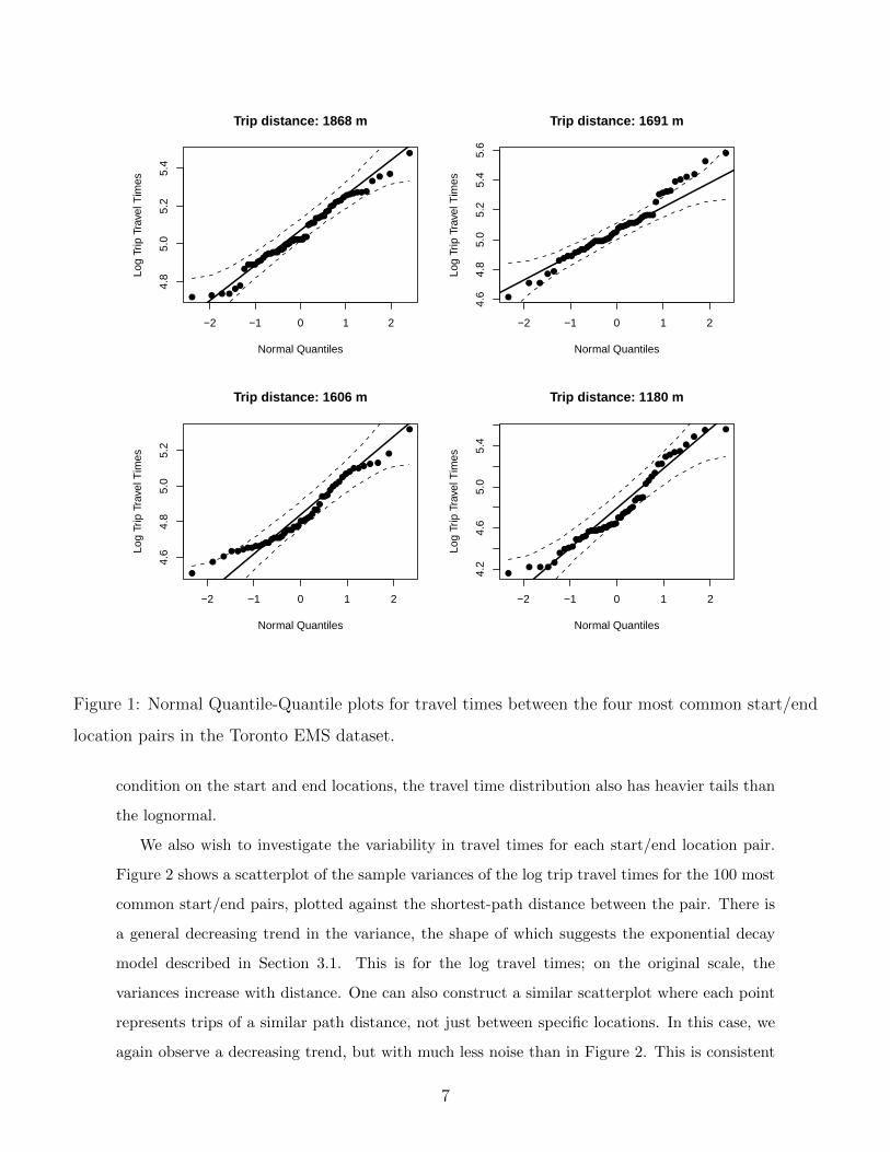
We also wish to investigate the variability in travel times for each start/end location pair.

Figure 2 shows a scatterplot of the sample variances of the log trip travel times for the 100 most

common start/end pairs, plotted against the shortest-path distance between the pair. There is

a general decreasing trend in the variance, the shape of which suggests the exponential decay

model described in Section 3.1. This is for the log travel times; on the original scale, the

variances increase with distance. One can also construct a similar scatterplot where each point

represents trips of a similar path distance, not just between specific locations. In this case, we

again observe a decreasing trend, but with much less noise than in Figure 2. This is consistent

7

●

●

●

●

●

●

●

●

●

●

●

●

●

●

●

●

● ●

● ●

●

●

●

●

●

●

●

●

●

●

●

●●

●

●

●

●

●

●

●

●

●

●

●●

●

●●

●

●

●

● ●

●

●

●

●

●●

●

●

●

●●

●

●

●

●

●

●

●●

●●

●

●

●

●

●

●

●

●●

●

●

●

●

●

● ●

●

●

●

●●

●

●

●

●

●

1000 2000 3000 4000

0.05

0.10

0.15

0.20

Trip distance (m)

Sam

ple

varia

nce

of lo

g tr

avel

tim

es

Figure 2: Sample variances of log travel times for the 100 most common start/end location pairs in

the Toronto EMS dataset.

with the results seen by Budge et al., who observed decreasing coefficient of variation of travel

times with increasing distance.

3 Modeling and Estimation

3.1 Travel Time Modeling

Consider a road network with links indexed by j ∈ {1, . . . , J} and a set of vehicle trips on that

network indexed by i ∈ {1, . . . , I}. Let dj indicate the length of link j. Assume that each trip i

begins and ends at known locations on the road network (not necessarily at intersections), and

that the sequence of links Ai = {Ai1, . . . , Aini} traversed by trip i is known. Let fij denote the

known fraction of link j used by trip i. For interior links in the path Ai, this fraction equals 1;

for the first and last links, it captures the fraction of the link actually traversed during the trip.

Based on the results of exploratory analysis in Section 2.1, we model the travel time Ti for

trip i with a lognormal distribution, conditional on the route traveled. Specifically,

Ti |Ai, {fij}j∈Ai , {dj}j∈Ai ∼ LN

µ(i) + log

c+∑j∈Ai

fijdju(i, j)

, σ2(i)

(1)

conditionally independent across trips i, where the functional forms of µ(i), u(i, j), and σ2(i)

8

are specified appropriately for the context. This model can be rewritten as Ti = Ri(c +∑j∈Ai

fijdju(i, j)) for a random lognormal multiplicative factor Ri ∼ LN (µ(i), σ2(i)) cap-

turing the travel time variability and trip-level effects. The baseline travel time is given by

(c+∑

j∈Aifijdju(i, j)), where the term u(i, j) is a unit travel time (inverse of speed) for trip i

on link j. The product fijdj is the distance traveled on link j in trip i, so the baseline travel

time is a sum of individual link travel times plus an intercept c > 0. One could also include

intersection and turn effects in the specification, although we have not pursued this extension.

The intercept c captures, for instance, additional time required to get up to speed at the

beginning of the trip and to slow down at the end. Its inclusion is similar to the model introduced

by Kolesar et al. [20] and used by Budge et al. [6], in which the travel times depend on the square

root of the distance for small distances, and grow linearly with the distance for large distances.

The unit travel time u(i, j) for link j in trip i can depend on explanatory factors like the road

class, speed limit, and whether the road is one-way. Additionally, it can depend on the type of

vehicle or the driver. Most simply it can be a link effect, giving the form u(i, j) , uj . However,

if there are links with very few trips, as is the case for ambulance data, this approach yields

noisy estimates of the uj parameters. We specify u(i, j) to depend on the road class, taking

u(i, j) , u`(j) where `(j) ∈ {1, . . . , L} is the road class of link j (highway, arterial road, etc.).

One could also partition the road network into R geographic regions, and take u(i, j) , u`(j),r(j)

for r(j) ∈ {1, . . . , R}, to allow downtown arterial roads to be distinguished from suburban

arterial roads, for example.

The parameters µ(i) and σ2(i) for the trip effect can depend on time, weather, driver, and

other explanatory factors (similarly to Jenelius et al. [17]). We use the time bin as an explanatory

factor, setting µ(i) , µk(i) where the week is divided into time bins k ∈ {0, 1, . . . ,K} and

µ0 , 0 to ensure model identifiability, i.e. so that each parameter of the model can be uniquely

determined given sufficient data.

The log scale variance σ2(i) is modeled via an exponential decay in the total trip distance di ,∑j∈Ai

fijdj , as suggested by exploratory data analysis (see Section 2.1, Figure 1). Specifically,

we take σ2(i) , Me−λdi + δ, for parameters M > 0, λ > 0, and δ > 0. With this choice, the

variance of the log travel times approaches δ as the trip distance increases, and equals M + δ

for trips of length zero. The parameter λ controls how quickly the variability decreases towards

δ. The unknown parameters in the model are therefore θ , (c, u1, . . . , uL, µ1, . . . , µK ,M, δ, λ).

9

3.2 Estimation

We use a Bayesian formulation to estimate the model parameters, which allows uncertainty in

the parameter estimates to be taken into account for travel time predictions. The predictions are

based on the posterior distribution of the parameters, which is proportional to the prior density

(specified below) times the likelihood function. The likelihood function is equal to the product

over trips i of the lognormal density of Ti (see Equation 1). We estimate each parameter and

relevant function of the parameters by its posterior mean, and summarize our uncertainty with a

95% interval estimate, the endpoints of which are the 0.025 and 0.975 quantiles of the posterior

distribution. Computation of the posterior distribution is done via Markov chain Monte Carlo

[34].

We have found results to be robust to moderate changes in the prior distributions for the

unknown parameters (c, u1, . . . , uL, µ1, . . . , µK ,M, δ, λ), due to the large volume of data. Results

are reported for the following prior distributions, with mutually independent parameters:

u` ∼ LN (ν`, ξ2u), µk ∼ N (0, ξ2µ), ` ∈ {1, . . . , L}, k ∈ {1, . . . ,K}

c ∼ Unif(0,∞),√M ∼ Unif(0,∞),

√δ ∼ Unif(0,∞), λ ∼ Unif(0,∞).

The constant ν` is a prior estimate of the unit travel time on the log scale, for road class `.

For example, there might be initial speed estimates for each link in class `, or perhaps known

speed limits or recorded GPS speed data. In such cases, ν` can be set equal to the mean of the log

inverse speeds. We use GPS speed data recorded during ambulance trips to specify a common

ν` for all `. The constant ξu captures how strongly we believe our prior estimate ν` of the log

unit travel time. We take ξu to be large, allowing the information in the data to dominate the

posterior estimate of u`. Specifically, we set ξu so that there is roughly 95% prior probability that

u` is within a factor of two of eν` , which corresponds to ξu = (log 2)/2. Similarly, ξµ captures

our prior uncertainty in the value of µk, and by the same argument we set ξµ = (log 2)/2. We

have no prior information about c, M , and δ, so we use uniform priors. Although these uniform

prior distributions are non-integrable, the posterior distribution is integrable and valid. The

uniform priors are on the square root of δ and M , because the square roots of these parameters

are on the scale of the standard deviation of the log travel times, and it is more appropriate to

put a uniform prior on a standard deviation than on a variance [10].

To estimate the posterior distribution for each parameter, we use a Metropolis-within-Gibbs

Markov chain Monte Carlo method [34]. Specifically, we use Metropolis-Hastings (M-H) to

10

update each of the unknown parameters in turn, conditional on the current values of the

other unknown parameters. For example, to update the parameter u`, we propose a new value

u∗` ∼ LN (log(u`), ψ2). The proposed sample is accepted with the appropriate M-H acceptance

probability, which is the minimum of 1 and the following product of the prior, likelihood, and

proposal density ratios:

LN (u∗` ; ν`, ξ2u)

LN (u`; ν`, ξ2u)

LN (u`; log(u∗` ), ψ2)

LN (u∗` ; log(u`), ψ2).

∏Ii=1 LN

(Ti;µk(i) + log

(c+

∑j∈Ai

fijdju∗`(j)

),Me−λdi + δ

)∏Ii=1 LN

(Ti;µk(i) + log

(c+

∑j∈Ai

fijdju`(j)

),Me−λdi + δ

) .The variance ψ2 is a constant that may be tuned to control the average acceptance probability,

which theoretical evidence suggests should be roughly 23% for optimal efficiency [31].

To obtain the results in this article, we ran each Markov chain for 120,000 iterations, including

a burn-in period of 20,000 iterations. To assess the Monte Carlo error, we calculated Monte

Carlo standard errors for each of the parameter estimates, using batch means [19]. Standard

errors are quite low, roughly 1-2% of the parameter estimate for the µk parameters and 0.03-0.2%

for the other parameters.

The computation time for each Markov chain iteration scales linearly with the number of

vehicle trips, for a fixed road network. Each Markov chain run for these experiments takes

roughly 18 hours on a personal computer, without utilizing parallel computing. Since the

likelihood is a product over the terms for each trip, computation time could be decreased by

calculating the likelihood terms in parallel batches. The Budge et al. nonparametric method [6] is

estimated using maximum (penalized) likelihood [30] and takes roughly 20 minutes on a personal

computer. In practice, however, ambulance travel time estimates are updated infrequently, so

increased computation time is not a severe drawback [37].

The reduced versions of our method (see Section 4.1) have smaller computation time than

the full method. For each set of parameters, the computation time is approximately linear in

the number of parameters. For example, the computation time for estimating the road class

parameters u` is reduced by approximately a factor of 7 for the model with only one road class,

compared to the full model with seven road classes. The computation time for estimating the

time bin parameters for the model with only one time bin is eliminated entirely, because the

first parameter µ0 is always fixed to 0. A model with two time bins has computation time for

estimating the time bin parameters reduced by approximately a factor of 3, compared to the

full model with four time bins.

11

4 Results

Here we give the results of ambulance travel time estimation using the Toronto data. We compare

our proposed method, our previous method described in [37], the nonparametric method of

Budge et al., and the TomTom predictions. For our proposed method, we use seven road classes

and four time bins. Class 1 corresponds to highways, Class 2 to major arterial roads, Classes

3-6 to smaller-sized roads in decreasing order, and Class 7 to highway on and off-ramps. These

road classes are derived from a digital map provided to us by Toronto EMS, although we have

consolidated some of the rarer classes. For example, there are multiple types of highway ramps

in the Toronto EMS map, which we have consolidated into one class. Classes 5-6 generally

represent local roads with little traffic, while Classes 2-4 represent different sizes of main roads.

Time Bin 0, the baseline bin, corresponds to weekday off-peak times (10 a.m. - 3 p.m., 7-10

p.m.), Bin 1 to rush hour (6-10 a.m., 3-7 p.m.), Bin 2 to weekend daytime (6 a.m. - 10 p.m.),

and Bin 3 to late night (10 p.m. - 6 a.m.). We chose these bins by observing the change in

average GPS speed readings across the week.

We split the ambulance trips randomly into two equal-sized sets, using half of the data to

train (estimate the parameters of) the statistical models, and the other half as test data for all

the methods. Then we reverse the training and test halves. Results from these two experiments

are similar. Table 1 gives parameter estimates from our method for the first training set.

The road class parameter estimates appear reasonable. The estimated unit travel time

u1 = 0.0353 s/m for Class 1 (highways) corresponds to approximately 102 km/hr. For Class

7 (highway on/off ramps), u7 = 0.0450 s/m corresponds to approximately 80 km/hr, and for

Class 2 (major arterial roads), u2 = 0.0603 s/m corresponds to approximately 60 km/hr. The

estimated speeds decrease for smaller roads, except for Class 6, the smallest roads. These roads

are relatively uncommon, and the interval estimate is wider for u6 than for the other parameters,

reflecting larger uncertainty in the value of u6.

The rush hour time bin parameter estimate µ1 = 0.0268 corresponds to a travel time increase

of about 2.7% for rush hour, relative to weekday off-peak. The estimates of µ2 and µ3 correspond

to roughly 1% smaller travel times for weekend and late night, relative to weekday off-peak. All

these values are close to zero, indicating that lights-and-sirens ambulance speeds are remarkably

consistent across time bins, in contrast to standard travel speeds [37].

Our lognormal model implies that about 95% of trips are predicted to fall within two standard

deviations of the median on the log scale, i.e. within factors of e−2×SD and e2×SD of the median

12

Parameter Description Estimate 95% posterior interval Speed Estimate

u1 Highway 0.0353 sec/m [0.0343, 0.0363] 102 km/hr

u2 Major arterial road 0.0603 sec/m [0.0600, 0.0606] 60 km/hr

u3 Large road 0.0653 sec/m [0.0648, 0.0659] 55 km/hr

u4 Medium road 0.0779 sec/m [0.0769, 0.0791] 46 km/hr

u5 Small road 0.1018 sec/m [0.0997, 0.1038] 35 km/hr

u6 Smallest road 0.0712 sec/m [0.0646, 0.0781] 51 km/hr

u7 Highway ramp 0.0450 sec/m [0.0426, 0.0476] 80 km/hr

µ1 Rush hour bin 0.0268 [0.0215, 0.0323] -

µ2 Weekend daytime bin -0.0083 [-0.0139, -0.0026] -

µ3 Late night bin -0.0097 [-0.0150, -0.0044] -

c Travel time intercept 25.08 sec [24.52, 25.66] -

M Variance parameter 0.2064 [0.1932, 0.2203] -

δ Variance parameter 0.0576 [0.0562, 0.0589] -

λ Variance parameter 0.00097 [0.00091, 0.00104] -

Table 1: Parameter estimates from our model, with 95% intervals expressing parameter uncertainty.

on the original scale. So the variance estimate δ = 0.0576 means that for very long trips about

95% of the travel times will be within factors of 0.62 and 1.6 of their median travel time. The

estimate M = 0.2064 implies that for very short trips about 95% of the travel times will be

within factors of 0.36 and 2.8 of their median travel time.

4.1 Travel Time Prediction Comparison

Next we compare the predictive performance for our method, several reduced versions of our

method, the nonparametric method of Budge et al. [6], and the TomTom estimates. Recalling

that we use half of the data for training and the other half for testing and then reverse, here

we evaluate the accuracy of the predicted travel time distribution for trips in the test data.

For details on the training of the Budge et al. method, see Appendix C. For each test trip we

evaluate the quality of a point estimate of the travel time, the predictive interval estimate, and

the distribution estimate using appropriate statistical measures. For TomTom we only evaluate

13

the quality of the point estimate since interval and distribution estimates are not available. For

the method of Budge et al., we use the median travel time as a point estimate. For our method,

we use the posterior mean of the median travel time as a point estimate. The 95% predictive

interval from those methods is taken to be the estimated 0.025 and 0.975 quantiles of the travel

time distribution.

When using our method to predict the travel time for the trips in the test data, we obtain

predictions under two scenarios: (1) using the estimated route taken by the vehicle (based on the

GPS data), or (2) not using this information. Using the estimated route emulates a situation in

which we know the route that the driver will take, for instance if the driver were required to take

a route specified by the dispatcher. Such control over the route could be desirable since then

the route could be optimally selected using the most recent traffic conditions. However, most

ambulance organizations leave the route choice to the driver, without notifying the dispatcher

of their choice. To emulate this situation, in Scenario 2 we predict the travel time without using

the route information (only using the start and end locations of the trip). In this scenario we

obtain an estimated fastest route according to our model (as described in Appendix B), and

base our predictions on this route.

Budge et al. base their travel time predictions on the shortest-path distance between the

start and end locations [6]. In the spirit of Scenario 1, since we have estimated routes for

each ambulance trip, it is natural to extend their method to use the distance of the estimated

route, instead of the shortest-path distance. Therefore, we obtain predictions from their original

method where the training and test sets both use the shortest-path distance, and the extended

method where the training and test sets both use the estimated route.

We perform bias correction for each estimation method, since bias may be present for a

variety of reasons. For example, bias arises in Scenario 2 introduced above because in this

scenario our method treats the ambulance paths differently in the training and test data. For

the training trips the estimated route is used, while for the test trips the fastest route is used,

resulting in a tendency to underestimate travel times. Bias may also be present in each method

due to inaccuracies of the assumed model. The TomTom estimates are severely biased, because

they are intended for vehicles traveling at standard speeds, not lights-and-sirens speeds. We

do bias correction on the log scale via cross-validation as described in previous work [37]. Bias

correction is done on the log scale to lessen the impact of outlying travel times.

Results are shown in Table 2. We report point estimation performance using the root mean

squared error (RMSE, in seconds) of the point estimate compared to the true time, and using

14

the RMSE of the log predictions compared to the true log time (“RMSE log”). Due to the

inherent variability in travel times, even a perfect distribution estimate would have RMSE and

RMSE log considerably above zero. We report the RMSE log because it is less affected by

outlying travel times than the RMSE. Outliers are present for at least two reasons; first, a small

number of trips were not driven at typical lights-and-sirens speeds, although they were recorded

as high-priority trips. Second, some trips have high error in the recorded GPS locations, in

which case the estimated path may be inaccurate.

Estimation method RMSE (s) RMSE log Cov. % Width (s) CRPS (s)

Our method, using estimated route 72.3 0.298 94.4 218.9 34.6

Our method, using fastest route 77.7 0.322 93.1 219.7 37.3

Our method, 1 variability parameter 72.5 0.297 94.1 225.9 35.2

Our method, 1 time bin 72.4 0.298 94.4 219.1 34.7

Our method, 1 road class 76.8 0.312 94.3 231.0 36.7

Extended Budge et al. 74.9 0.302 94.6 229.1 35.7

Budge et al. 79.7 0.325 94.8 248.1 38.3

TomTom 82.1 0.347 NA NA NA

Table 2: Travel time prediction performance for the Toronto EMS lights-and-sirens data.

To evaluate the interval estimates, Table 2 shows the percentage of test trips where the

observed travel time falls in the 95% predictive interval (the coverage, “Cov. %”), as well as

the geometric mean width of the 95% predictive intervals (“Width”). Coverage close to or

above 95% combined with small interval width is desirable, since it indicates that the predictive

distribution is narrowly concentrated around the true travel time, while reflecting the true

variability in travel times.

Table 2 evaluates the quality of the distribution estimates by reporting the continuous ranked

probability score (CRPS) [11]. This is a “strictly proper” measure of distribution estimation

accuracy, meaning that only a perfect distribution estimate achieves the lowest expected score

[12]. If F is the estimated distribution function and x is the observed travel time, CRPS(F ;x) ,∫∞−∞ [F (y)− 1(y ≥ x)]2 dy is the integrated square of the difference between F and the empirical

distribution function based on the single observation x [11]. A lower value corresponds to a better

distribution estimate. Even a perfect distribution estimate would yield a CRPS value well above

15

zero, due to the inherent variability of travel times. We report the mean CRPS over the test

trips [11].

In Table 2, in addition to reporting the accuracy of our method under Scenarios 1 and 2, and

the accuracy of the competing methods, we report the accuracy of several simplified versions

of our method under Scenario 1. This indicates whether the simplified models are as effective

as our full model and which aspects of our full model are the most important. We consider

the following simplifications: (a) only one time bin, (b) only one road class, and (c) only one

variability parameter instead of the exponential model.

As seen in Table 2, our method under Scenario 1 (using the estimated route) outperforms the

Budge et al. method by 8-10% in RMSE, RMSE log, and CRPS, and outperforms the extended

Budge et al. method by 1.5-3.5% in the same metrics. Our method’s interval estimates have

almost identical coverage to those of Budge et al. but are narrower on average, by 12% compared

to the original Budge et al. method and by 4.5% compared to the extended method. Under

Scenario 2, our method outperforms the original Budge et al. method by 2.6% in CRPS and

1-3% in RMSE and RMSE log. Our mean predictive interval width under this scenario is 11%

narrower than that of Budge et al., though with slightly lower coverage. These performance

differences are most likely due to our model’s inclusion of different speeds for the different road

classes, as well as time effects.

Our method outperforms the TomTom estimates by 12-14% in RMSE and RMSE log under

Scenario 1, and by 5-7% in the same metrics under Scenario 2. Scenario 2 is the more natural

comparison, because we do not specify the route traveled when obtaining the TomTom estimates,

instead allowing TomTom to pick the optimal route. TomTom’s estimates perform respectably,

indicating that after bias correction, standard vehicle data do have predictive power for lights-

and-sirens ambulance trips.

Regarding the reduced versions of our approach, the method with only one time bin performs

essentially as well in all metrics as the full method. This observation agrees with results from

other studies, which found that travel times of emergency vehicles were not strongly influenced

by time-of-day [1, 20]. We investigated this observation further by artificially inflating the travel

times during rush hour, and found that the method with only one time bin still performed almost

as well as the full method (2% worse RMSE) when the rush hour travel times were inflated by

10%. The model with only one variability parameter performs as well in point estimation but

slightly worse in distribution estimation than the full model.

The method with only one road class performs worse than the full method and the other

16

reduced methods in all metrics. Therefore, it is quite important to allow for varying speeds

across road classes (see previous work [37]). We also investigated methods with two and four

road classes (not shown), and found that the largest benefit arose from moving from one to two

road classes (highway and non-highway). Moving from two to four road classes and from four to

seven road classes gave smaller improvements. The extended Budge et al. method outperforms

our method with one road class. Both models rely only on travel distance; however, the Budge

et al. method is more flexible than our method with one road class, because the point estimates

on the log scale are not restricted to a linear function of distance.

4.2 Comparison to our Previous Method

We also wish to compare to our earlier method as described in [37], referred to as Westgate et al.

Our previous method is much more computationally intensive than the method proposed here

because it simultaneously estimates the routes of the historical trips and travel time parameters

of each network link. Because of this, we cannot apply it to the entire Toronto road network,

so we compare our new method to our previous method on the subregion of Leaside, Toronto.

To ensure a fair comparison, we do not use the route information for the test trips with either

method (i.e., we use Scenario 2 from Section 4.1).

For application to the subregion we make one minor change to the model introduced in

Section 3.1. For the prior distribution on the variance parameter M , we use an exponential

distribution with rate 5, instead of a uniform distribution. Since the dataset has few extremely

short trips, posterior estimates of M are unstable unless we use a prior distribution that prefers

smaller values. Failure to do this can lead to unrealistic travel time predictions for the few

extremely short trips in the dataset.

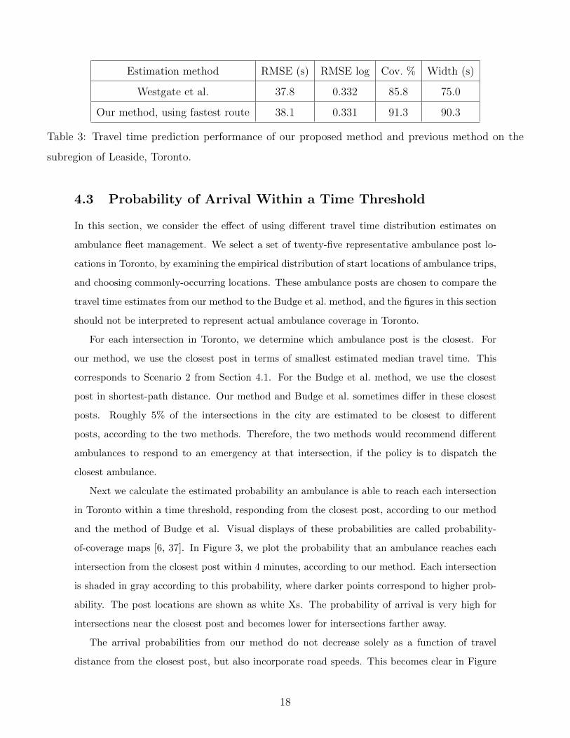
Results are summarized in Table 3. We use the same five resamplings of training and test

sets from the Toronto subregion data as in [37]. The two methods perform roughly the same

in terms of RMSE log, and our previous method performs only slightly better than our new

method in RMSE, even though the new method is much less computationally intensive. Our new

method also has much better coverage of interval estimates than our previous method. This

is because our previous method assumed independence between the travel times on different

network links, which is unrealistic, as discussed in Section 1. Failing to take into account the

association between link travel times leads to underestimation of the variability in the total

route travel time and thus overly narrow interval estimates.

17

Estimation method RMSE (s) RMSE log Cov. % Width (s)

Westgate et al. 37.8 0.332 85.8 75.0

Our method, using fastest route 38.1 0.331 91.3 90.3

Table 3: Travel time prediction performance of our proposed method and previous method on the

subregion of Leaside, Toronto.

4.3 Probability of Arrival Within a Time Threshold

In this section, we consider the effect of using different travel time distribution estimates on

ambulance fleet management. We select a set of twenty-five representative ambulance post lo-

cations in Toronto, by examining the empirical distribution of start locations of ambulance trips,

and choosing commonly-occurring locations. These ambulance posts are chosen to compare the

travel time estimates from our method to the Budge et al. method, and the figures in this section

should not be interpreted to represent actual ambulance coverage in Toronto.

For each intersection in Toronto, we determine which ambulance post is the closest. For

our method, we use the closest post in terms of smallest estimated median travel time. This

corresponds to Scenario 2 from Section 4.1. For the Budge et al. method, we use the closest

post in shortest-path distance. Our method and Budge et al. sometimes differ in these closest

posts. Roughly 5% of the intersections in the city are estimated to be closest to different

posts, according to the two methods. Therefore, the two methods would recommend different

ambulances to respond to an emergency at that intersection, if the policy is to dispatch the

closest ambulance.

Next we calculate the estimated probability an ambulance is able to reach each intersection

in Toronto within a time threshold, responding from the closest post, according to our method

and the method of Budge et al. Visual displays of these probabilities are called probability-

of-coverage maps [6, 37]. In Figure 3, we plot the probability that an ambulance reaches each

intersection from the closest post within 4 minutes, according to our method. Each intersection

is shaded in gray according to this probability, where darker points correspond to higher prob-

ability. The post locations are shown as white Xs. The probability of arrival is very high for

intersections near the closest post and becomes lower for intersections farther away.

The arrival probabilities from our method do not decrease solely as a function of travel

distance from the closest post, but also incorporate road speeds. This becomes clear in Figure

18

Figure 3: Probability of arriving at each intersection in Toronto from the closest ambulance post

within 4 minutes, estimated by our method.

4, where we plot the differences between the arrival probabilities for our method and the Budge

et al. method. The black points represent intersections where our method gives at least 15

percentage points higher probability of arrival within 4 minutes than the Budge et al. method

does. Thus, there is a substantial predictive difference between the two distributions for these

intersections. The medium grey points are intersections where the Budge et al. method gives at

least 15 percentage points higher probability than our method does. The light gray points are

all other intersections. The ambulance post locations are shown as black Xs.

Most of the intersections that are close to an ambulance post do not differ by 15 percentage

points or more according to the two methods, because arrival probabilities from both methods

19

Figure 4: Differences in the estimated probability of arriving within 4 minutes, between our method

and that of Budge et al.

are high. Similarly, intersections that are far from all ambulance posts also differ by less than

15 percentage points. On the other hand, many of the intersections that are at an intermediate

distance to the closest ambulance post differ in arrival probability by 15 percentage points or

more. In fact, this is true for roughly 10% of all the intersections in the city. Many of the points

where the probability from our method is at least 15 percentage points higher are on or near

highways, particularly Highway 401, which is visible in Figure 4 as a sequence of black points

running horizontally across the middle of the city. The highway road class speed estimate is

high, so the method predicts better coverage when a highway can be used. There is another

large collection of black points at the left edge of the figure that are close to Highway 427.

Many of the intersections where the Budge et al. probability is at least 15 percentage points

20

higher are in residential areas where there is no direct path following highways or major arterial

roads. For example, there are no major roads traveling from an ambulance post to the collection

of gray points near location (-10000, -7000). Similarly, there is no direct route from an ambulance

post to the collection of gray points near location (-5000, 7000). Though there are major arterial

roads in the area, it would require a detour to use one. There are smaller roads that take more

direct routes from the ambulance posts, but these road classes have slower speed estimates.

5 Conclusions

We introduced a parametric model for estimating the distribution of ambulance travel times

between any locations in a road network. The method uses data from historical ambulance trips

that can be sparse in time and network coverage, and is computationally tractable for large

road networks and large datasets of vehicle trips. The model parameters are interpretable, and

include effects for the roads traveled by the vehicle and trip-level effects such as time of day.

We used a Bayesian formulation and Markov chain Monte Carlo method to estimate the model

parameters.

We tested the method on a large dataset of ambulance trips from Toronto. Exploratory

analysis of the data indicated that the distribution of ambulance travel times between two fixed

locations is well modeled by a lognormal distribution, with variability parameter depending on

travel distance. These observations influenced our modeling choices. We compared travel time

predictions from our method with predictions from a recently-published method by Budge et al.

[6] and commercially available travel time estimates from TomTom. We found that our method

outperformed the alternative methods in both point estimation and distribution estimation. We

also compared our method with the method of Westgate et al. [37] on a subregion of Toronto,

and found that our method performed almost as well in point estimation and better in interval

estimation, while being far more computationally efficient.

We also investigated several reduced versions of our method, to determine which features

were the most important. The largest benefit came from the inclusion of parameters for each

road class in the city, compared to a model with only one road class. However, there was little

benefit in performance from adding multiple time bins across the week vs. a single time bin. In

the Toronto dataset, the ambulance travel times do not vary substantially across the day and

week, even during rush hour. Because other cities or datasets may be more variable in time, we

performed an additional set of experiments by artificially inflating the difference in travel times

21

between time bins. We found that if the travel times during rush hour were increased by at

least 20%, then time bin factors provided a substantial benefit to estimation.

Finally, we investigated operational differences for ambulance fleet management from using

our method vs. the method of Budge et al. After fixing a set of representative ambulance posts

in Toronto, we calculated the probability that an ambulance arrives at each intersection in the

city within 4 minutes, responding from the closest post. We found that for about 10% of the

intersections in the city, the two methods gave arrival probabilities that differed by more than

15 percentage points.

A Preprocessing

For each ambulance trip we have the time the ambulance departed for the scene (enroute time),

the arrival time, and GPS readings for the ambulance between those two times. Ideally, we

would use the difference between the enroute and arrival times as the total trip travel time, and

use the GPS readings between the enroute and arrival times to estimate the path traveled via

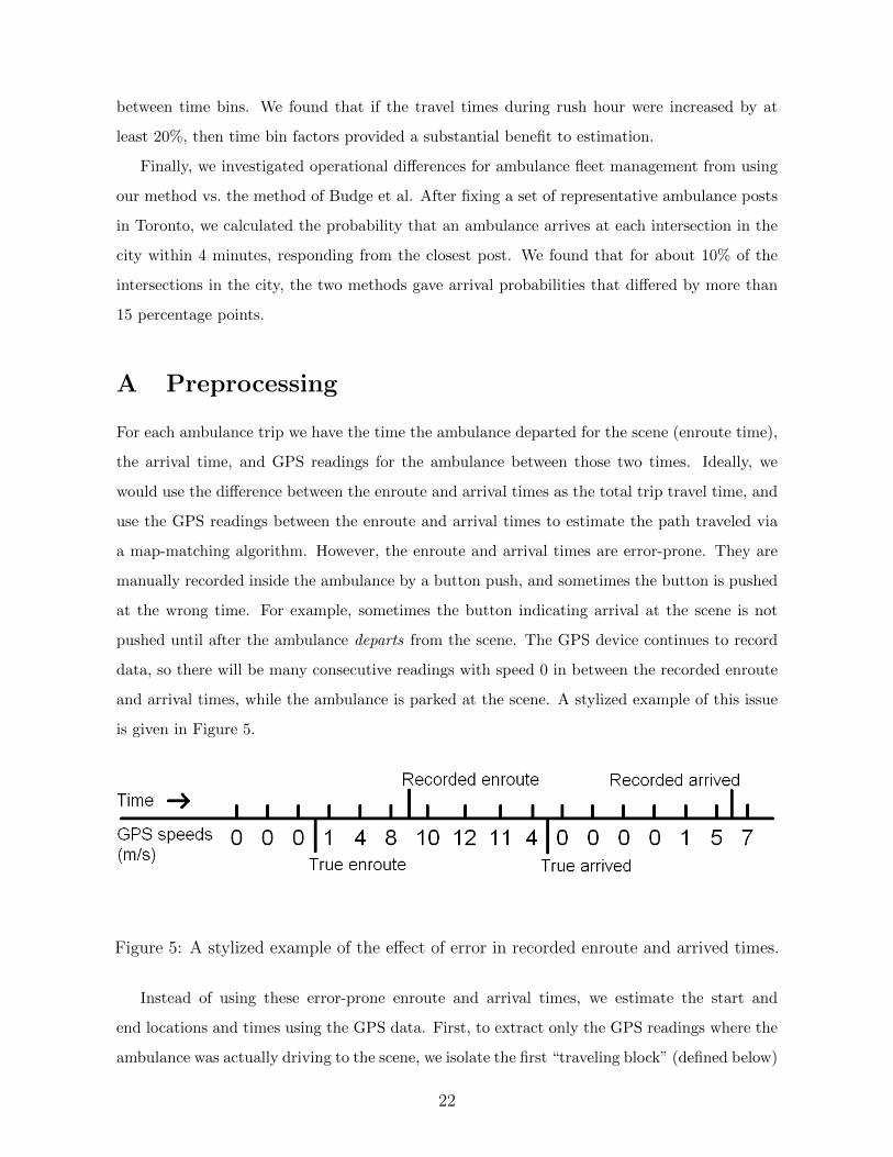
a map-matching algorithm. However, the enroute and arrival times are error-prone. They are

manually recorded inside the ambulance by a button push, and sometimes the button is pushed

at the wrong time. For example, sometimes the button indicating arrival at the scene is not

pushed until after the ambulance departs from the scene. The GPS device continues to record

data, so there will be many consecutive readings with speed 0 in between the recorded enroute

and arrival times, while the ambulance is parked at the scene. A stylized example of this issue

is given in Figure 5.

Figure 5: A stylized example of the effect of error in recorded enroute and arrived times.

Instead of using these error-prone enroute and arrival times, we estimate the start and

end locations and times using the GPS data. First, to extract only the GPS readings where the

ambulance was actually driving to the scene, we isolate the first “traveling block” (defined below)

22

of GPS points, and discard the rest. Then we take the first and last GPS points of the traveling

block as the estimated start and end locations and times of the trip. Due to GPS measurement

error, these locations are not necessarily on the road network, but the map-matching algorithm

we use can handle this discrepancy [36].

Our preprocessing method is the following:

1. For each incident in which the ambulance responds at lights-and-sirens speeds, extract all

GPS points with timestamps between the recorded enroute and arrived times.

2. For each trip, retain the first “traveling block” of GPS points, discarding the rest.

Traveling block: A maximal consecutive sequence of GPS readings, with the requirements:

1. Begins and ends with a non-zero GPS speed.

2. Has at least 3 non-zero speed GPS readings.

3. Has no pair of GPS readings (consecutive or otherwise) with:

(a) Timestamps at least 30 seconds apart but with average speed < 1.8 km/hr, using

straight-line distance.

(b) Timestamps at least 2 minutes apart but with average speed < 7.2 km/hr, using

straight-line distance.

(c) Average speed (straight-line) greater than 360 km/hr.

4. Has straight-line distance of at least 400 m between the first and last GPS readings.

5. Has average speed (based on straight-line distance) between the first and last GPS readings

no greater than 216 km/hr.

Each of these requirements are designed to eliminate a certain type of error. Requirement

1 removes zero-speed GPS readings at the beginning or end of the trip. Requirement 2 ensures

that we can estimate start and end locations for the trip, with at least one additional GPS read-

ing for path estimation. Requirement 3 ensures that the trip does not have a long stationary

period in the middle, as in Figure 5. This requirement also removes trips where the ambulance

turned around, and subsequent GPS readings are very close to each other. While this is pos-

sible behavior, it is unhelpful for response time estimation to include these trips. Finally, this

requirement also removes trips with severe errors in the GPS timestamp or location. Errors

in the GPS data are not common, but occasionally the data contain successive GPS readings

with identical timestamps but different locations, or GPS readings with impossible locations.

23

Requirements 4 and 5 act similarly to Requirement 3, but on the entire trip. Requirement 4

removes trips where the ambulance turned around and the first and last GPS reading are very

close to each other. Requirement 5 removes rare trips where the GPS data are shifted by a very

large amount from the true location.

B Fastest Path Estimation

Here we describe the fastest path estimation for our method under Scenario 2 of Section 4.1. As

noted in Appendix A, the recorded start and end times for the ambulance trips are error-prone,

so the first and last GPS readings in the first traveling block of the trip are used for the start and

end times and locations. Since these two locations are not necessarily on the road network, to

estimate the fastest path we first find the two nearest links to these GPS locations, and use the

nearest points on these links as possible start/end locations. These links typically correspond

to the two travel directions of the nearest road. For each of the four start/end location pairs,

we calculate the fastest path in median travel time. Of these four possible paths, we use the

one with the smallest median travel time as the estimated path. This method ensures that we

obtain a reasonable path for each trip, which can begin or end in the interior of a link, and is

not hampered by choosing the “wrong direction” of the nearest link.

C Implementation of Budge et al.

In this section, we give details of our implementation of the nonparametric method of Budge

et al [6]. For trip i, with travel time Ti and shortest-path distance di, Budge et al. use the

model log(Ti) = log(m(di))+ c(di)εi, where εi follows a t-distribution with τ degrees of freedom.

They introduced a parametric method and a nonparametric method for estimating m(di) and

c(di). We chose to implement their nonparametric method, because they proposed the para-

metric method for ease of interpretation, and concluded that results from the nonparametric

method were slightly superior to the results from the parametric method, in terms of the Akaike

Information Criterion (AIC) [5].

To implement the Budge et al. nonparametric method, we used the R package GAMLSS [33].

Plots of the fitted median and coefficient of variation functions, for one half of our dataset (the

training data), are given in Figure 6. The plots also include 95% bootstrap confidence bands

(pointwise) for the two functions. Distance is measured in kilometers (km) and time in minutes

24

(min.), for ease of comparison to the results of Budge et al.

Comparing these plots to Figure 3 of Budge et al., we observe similar behavior in the rela-

tionship between travel time and shortest-path distance. The median travel time function for

our data increases between 0 and 10 km, with slightly decreasing slope, and the coefficient of

variation decreases from 0.5 to slightly above 0.2 in that range, as in Budge et al. Our dataset

contains some trips with distance longer than 10 km, while the dataset of Budge et al. does not.

However, these trips are rare in our data. Although our entire dataset is large (157,283 trips),

our training data contain only 463 trips with distances greater than 10 km and 45 trips with

distances greater than 15 km. For these distances, the median travel time function grows more

slowly and then more quickly, while the coefficient of variation grows and then decreases. The

confidence bands also widen substantially.

0 5 10 15 20 25

05

1015

20

Distance (km)

Med

ian

trav

el ti

me

(min

.)

0 5 10 15 20 25

0.1

0.2

0.3

0.4

0.5

0.6

Distance (km)

Coe

ffici

ent o

f var

iatio

n

Figure 6: Median and coefficient of variation functions for ambulance travel times, estimated by the

Budge et al. nonparametric method.

Both the median and coefficient of variation functions for our data have non-monotonic

fluctuations, though these are much more pronounced for the coefficient of variation. These

fluctuations remain regardless of the parameters used in implementing the GAMLSS function.

This is an artifact of the large size of our dataset (157,283 trips, compared to 6886 for Budge

et al.). If a random subset of 10,000 trips is drawn from our dataset, for example, the resulting

25

functions do not show these fluctuations.

Our results differ from those of Budge et al. in the estimated degrees of freedom τ of the

t-distribution. The non-parametric method of Budge et al. estimated τ = 3.71 for their data,

whereas for our data the estimate is τ = 10.6. This difference may arise because of the different

preprocessing methods between our two applications (more outliers in the Budge et al. data

would lead to a heavier-tailed distribution), or from fundamental differences in the travel time

characteristics between the two cities. We confirmed this observation by binning the travel

times in our data by distance, as Budge et al. did in their preliminary analysis, and fitting

t-distributions to the log travel times in each bin. The fitted degrees of freedom for our data

ranged from 5.1 to 172 for the different bins, with a median of 10.9.

Acknowledgements

We thank Christopher Glessner for his work obtaining the TomTom estimates. We also thank

Toronto EMS, Dave Lyons, TomTom, and The Optima Corporation. This research was partially

supported by NSF Grant CMMI-0926814, NSF Grant DMS-1209103, NSF Grant DMS-1455172,

and a Xerox PARC faculty research award.

References

[1] K. Aladdini. EMS response time models: A case study and analysis for the region of

Waterloo. Master’s thesis, University of Waterloo, 2010.

[2] R. Alanis, A. Ingolfsson, and B. Kolfal. A Markov chain model for an EMS system with

repositioning. Production and Operations Management, 22:216–231, 2013.

[3] M. Bernard, J. Hackney, and K.W. Axhausen. Correlation of link travel speeds. In 6th

Swiss Transport Research Conference. Ascona, Switzerland, 2006.

[4] L. Brotcorne, G. Laporte, and F. Semet. Ambulance location and relocation models. Eu-

ropean Journal of Operational Research, 147:451–463, 2003.

[5] S. Budge, A. Ingolfsson, and D. Zerom. Electronic companion to “Empirical analysis of

ambulance travel times: The case of Calgary emergency medical services”. Management

Science, 56:716–723, 2010.

26

[6] S. Budge, A. Ingolfsson, and D. Zerom. Empirical analysis of ambulance travel times: The

case of Calgary emergency medical services. Management Science, 56:716–723, 2010.

[7] S.F. Dean. Why the closest ambulance cannot be dispatched in an urban emergency medical

services system. Prehospital and Disaster Medicine, 23:161–165, 2008.

[8] E. Erkut, R. Fenske, S. Kabanuk, Q. Gardiner, and J. Davis. Improving the emergency

service delivery in St. Albert. Infor, 39:416–433, 2001.

[9] E. Erkut, A. Ingolfsson, and G. Erdogan. Ambulance location for maximum survival. Naval

Research Logistics (NRL), 55:42–58, 2008.

[10] A. Gelman. Prior distributions for variance parameters in hierarchical models. Bayesian

Analysis, 1:515–533, 2006.

[11] T. Gneiting, F. Balabdaoui, and A.E. Raftery. Probabilistic forecasts, calibration and

sharpness. Journal of the Royal Statistical Society: Series B, 69:243–268, 2007.

[12] T. Gneiting and A.E. Raftery. Strictly proper scoring rules, prediction, and estimation.

Journal of the American Statistical Association, 102:359–378, 2007.

[13] J.B. Goldberg. Operations research models for the deployment of emergency services vehi-

cles. EMS Management Journal, 1:20–39, 2004.

[14] A. Hofleitner, R. Herring, P. Abbeel, and A. Bayen. Learning the dynamics of arterial traffic

from probe data using a dynamic Bayesian network. IEEE Transactions on Intelligent

Transportation Systems, 13:1679–1693, 2012.

[15] A. Hofleitner, R. Herring, and A. Bayen. Arterial travel time forecast with streaming data:

A hybrid approach of flow modeling and machine learning. Transportation Research Part

B, 46:1097–1122, 2012.

[16] A. Ingolfsson, S. Budge, and E. Erkut. Optimal ambulance location with random delays

and travel times. Health Care Management Science, 11:262–274, 2008.

[17] E. Jenelius and H.N. Koutsopoulos. Travel time estimation for urban road networks using

low frequency probe vehicle data. Transportation Research Part B, 53:64–81, 2013.

[18] I. Kaparias, M.G.H. Bell, and H. Belzner. A new measure of travel time reliability for

in-vehicle navigation systems. Journal of Intelligent Transportation Systems, 12:202–211,

2008.

27

[19] W.D. Kelton and A.M. Law. Simulation Modeling and Analysis. McGraw Hill, Boston,

2000.

[20] P. Kolesar, W. Walker, and J. Hausner. Determining the relation between fire engine travel

times and travel distances in New York City. Operations Research, 23:614–627, 1975.

[21] Y. Lou, C. Zhang, Y. Zheng, X. Xie, W. Wang, and Y. Huang. Map-matching for low-

sampling-rate GPS trajectories. In Proceedings of the 17th ACM SIGSPATIAL Interna-

tional Conference on Advances in Geographic Information Systems, pages 352–361. ACM,

New York, 2009.

[22] A.J. Mason. Emergency vehicle trip analysis using GPS AVL data: A dynamic program for

map matching. In Proceedings of the 40th Annual Conference of the Operational Research

Society of New Zealand, pages 295–304. Wellington, NZ, 2005.

[23] M.S. Maxwell, M. Restrepo, S.G. Henderson, and H. Topaloglu. Approximate dynamic

programming for ambulance redeployment. INFORMS Journal on Computing, 22:266–281,

2010.

[24] E. Mazloumi, G. Currie, and G. Rose. Using GPS data to gain insight into public transport

travel time variability. Journal of Transportation Engineering, 136:623–631, 2009.

[25] L.A. McLay. Emergency medical service systems that improve patient survivability. In

Wiley Encyclopedia of Operations Research and Management Science. Wiley, New York,

2010.

[26] J.Y. Potvin, Y. Xu, and I. Benyahia. Vehicle routing and scheduling with dynamic travel

times. Computers & Operations Research, 33:1129–1137, 2006.

[27] M.A. Quddus, W.Y. Ochieng, and R.B. Noland. Current map-matching algorithms for

transport applications: State-of-the art and future research directions. Transportation

Research Part C, 15:312–328, 2007.

[28] M. Rahmani and H.N. Koutsopoulos. Path inference from sparse floating car data for urban

networks. Transportation Research Part C, 30:41–54, 2013.

[29] M. Ramezani and N. Geroliminis. On the estimation of arterial route travel time distribu-

tion with Markov chains. Transportation Research Part B, 46:1576–1590, 2012.

[30] R.A. Rigby and D.M. Stasinopoulos. Generalized additive models for location, scale and

shape. Journal of the Royal Statistical Society: Series C, 54:507–554, 2005.

28

[31] G.O. Roberts and J.S. Rosenthal. Optimal scaling for various Metropolis-Hastings algo-

rithms. Statistical Science, 16:351–367, 2001.

[32] V. Schmid. Solving the dynamic ambulance relocation and dispatching problem using

approximate dynamic programming. European Journal of Operational Research, 219:611–

621, 2012.

[33] D.M. Stasinopoulos and R.A. Rigby. Generalized additive models for location scale and

shape (GAMLSS) in R. Journal of Statistical Software, 23:1–46, 2007.

[34] L. Tierney. Markov chains for exploring posterior distributions. The Annals of Statistics,

22:1701–1728, 1994.

[35] H. Topaloglu. A parallelizable dynamic fleet management model with random travel times.

European Journal of Operational Research, 175:782–805, 2006.

[36] B.S. Westgate. Vehicle Travel Time Distribution Estimation and Map-Matching Via

Markov Chain Monte Carlo Methods. PhD thesis, Cornell University, 2013.

[37] B.S. Westgate, D.B. Woodard, D.S. Matteson, and S.G. Henderson. Travel time estimation

for ambulances using Bayesian data augmentation. Annals of Applied Statistics, 7:1139–

1161, 2013.

[38] J. Yuan, Y. Zheng, C. Zhang, W. Xie, X. Xie, G. Sun, and Y. Huang. T-drive: driving

directions based on taxi trajectories. In Proceedings of the 18th SIGSPATIAL International

Conference on Advances in Geographic Information Systems, pages 99–108. ACM, 2010.

[39] L. Zhen, K. Wang, H. Hu, and D. Chang. A simulation optimization framework for ambu-

lance deployment and relocation problems. Computers & Industrial Engineering, 72:12–23,

2014.

29