RESEARCH ARTICLE

Travel distance estimation from visual motion by leakypath integration

Markus Lappe Æ Michael Jenkin Æ Laurence R. Harris

Received: 25 September 2006 / Accepted: 13 December 2006 / Published online: 13 January 2007� Springer-Verlag 2007

Abstract Visual motion can be a cue to travel dis-

tance when the motion signals are integrated. Distance

estimates from visually simulated self-motion are

imprecise, however. Previous work in our labs has gi-

ven conflicting results on the imprecision: experiments

by Frenz and Lappe had suggested a general under-

estimation of travel distance, while results from Red-

lick, Jenkin and Harris had shown an overestimation of

travel distance. Here we describe a collaborative study

that resolves the conflict by tracing it to differences in

the tasks given to the subjects. With an identical set of

subjects and identical visual motion simulation we

show that underestimation of travel distance occurs

when the task involves a judgment of distance from the

starting position, and that overestimation of travel

distance occurs when the task requires a judgment of

the remaining distance to a particular target position.

We present a leaky integrator model that explains both

effects with a single mechanism. In this leaky integra-

tor model we introduce the idea that, depending on the

task, either the distance from start, or the distance to

target is used as a state variable. The state variable is

updated during the movement by integration over the

space covered by the movement, rather than over time.

In this model, travel distance mis-estimation occurs

because the integration leaks and because the trans-

formation of visual motion to travel distance involves a

gain factor. Mis-estimates in both tasks can be ex-

plained with the same leak rate and gain in both con-

ditions. Our results thus suggest that observers do not

simply integrate traveled distance and then relate it to

the task. Instead, the internally represented variable is

either distance from the origin or distance to the goal,

whichever is relevant.

Keywords Visual motion � Path integration �Human � Distance perception � Self motion

Introduction

The sensory basis of knowledge of one’s own positition

during locomotion consists of proprioceptive, vestibu-

lar, and visual signals. Vision may support the knowl-

edge of one’s own positition by relationship to known

landmarks in the environment (Judd and Collet 1998;

Gillner and Mallot 1998), or by providing visual mo-

tion cues about direction, speed, and duration of

movement, which must be integrated to achieve a

measure of the distance traveled (Peruch et al. 1997;

Bremmer and Lappe 1999; Riecke et al. 2002). Such

integration may be similar to the integration of ves-

tibular or proprioceptive inputs in the process of path

integration (Mittelstaedt and Mittelstaedt 1980).

Path integration estimates the course of an extended

movement by integrating short pieces of the movement

to yield the total path (Mittelstaedt and Mittelstaedt

1973; Maurer and Seguinot 1995). If the path involves

turns, the direction and amount of turn are also taken

into account. Path integration has been studied

extensively with blindfolded subjects in order to

determine the ability to use proprioceptive and

M. Lappe (&)Psychological Institute II, Westf. Wilhelms-University,Fliednerstr. 21, 48149 Munster, Germanye-mail: mlappe@psy.uni-muenster.de

M. Jenkin � L. R. HarrisCenter for Vision Research, York University,Toronto, Canada

123

Exp Brain Res (2007) 180:35–48

DOI 10.1007/s00221-006-0835-6

vestibular cues for the estimation of path length and

turns (Loomis et al. 1993; Etienne et al. 1996; Loomis

et al. 1999).

Visual motion cues also support the estimation of

travel distance. Human observers are quite accurate in

discriminating the path length of two visually simulated

forward motions even when the velocities of the two

motions differ (Bremmer and Lappe 1999). The ability

to visually discriminate two path lengths is not trivial

because optic flow, the visual velocity pattern gener-

ated by self motion, is ambiguous without information

about the scale of the visual environment. When the

distances to all visual elements are increased by a

particular factor, and the forward speed is multiplied

by the same factor, then the visual speeds in the optic

flow in terms of degrees per second remain the same.

Thus the ability to discriminate the distances of two

simulated self-motions must rely on knowledge of the

relationship between the environments.

Clearly discernable changes of the view of the

environment between two succesive self-motions (such

as a visible increase in eye height above the ground)

can be used to re-scale the use of the optic flow

information to allow accurate discrimination also be-

tween environments (Frenz et al. 2003). This suggests

that path length estimation from visual motion is based

on an estimate of one’s own velocity relative to the

environment rather than directly on the pattern of

optic flow. This estimate of self-velocity, however, has

to be derived from the optic flow information.

Knowing one’s own position in the environment

after a period of movement requires more than being

able to discriminate movement distances. One needs to

convert the absolute estimated movement distance to

an updated position. This requires explicit use of the

scale of the environment. Experimental investigation

of an observer’s ability to convert absolute movement

distances to an updated position involves relating a

particular movement to a particular target position.

Redlick et al. (2001) presented participants with an

initial target at a given distance within a visually sim-

ulated hallway, then extingushed the target and sub-

sequently used optic flow to simulate a movement

towards the now invisible target. Participants indicated

the point when they felt that they had arrived at the

target position. From this, the simulated travel distance

was calculated that perceptually matched the visual

distance to the initially shown target. For constant

velocity movement, participants usually responded too

early. For instance, for an initial target distance of

16 m they responded when they had travelled only

12 m. This suggests that the travel distance was over-

estimated: with a true movement of 12 m subjects felt

they had covered the distance to the target that was

initially 16 m away.

Frenz and Lappe (2005) conducted similar experi-

ments but with a reversed order procedure. First,

participants experienced a simulated movement of a

given distance over a flat terrain. Then they adjusted a

target to match the distance of the simulated move-

ment. Participants on average placed the target too

close. For instance, for a true movement of 5.5 m they

placed the target at 4 m. This suggests that the simu-

lated travel distance was underestimated. Such under-

estimation was found independently of the depth cues

provided in the visual environment and of the report-

ing measure used (target adjustment, walking the same

distance blindfolded, verbal distance in multiples of

height above ground) (Frenz and Lappe 2005; Lappe

et al. 2005).

Frenz and Lappe (2005) reproduced the overesti-

mation found by Redlick et al. (2001) when they used

the experimental procedure of showing the target first

and requiring subjects to report the arrival at the tar-

get, as was done in the Redlick et al. study. However,

this was only true for large target distances. When the

procedure of Redlick et al. (2001) was used with small

target distances, an underestimation of travel distance

was observed.

In order to resolve this apparent incompatibility

between the two data sets, we compared travel distance

estimates in both experimental procedures over a large

range of distances using the same equipment and

subjects. We show that travel distance estimates are

similar in both paradigms for short distances but

become very dissimilar for large distances. We propose

a path integration model based on leaky integration

over the covered space that can explain all these

observations.

Methods

Participants

10 subjects (3 females, 7 males, between 20 and

53 years old) participated in the study. All had normal

or corrected-to-normal vision. All experiments were

approved by the York University Human Experiment

Subject Committee.

Setup and stimuli

The experiments were conducted in the Immersive

Visual Environment at York University (IVY, Robin-

son et al. 2002). The subject was seated in the center of

36 Exp Brain Res (2007) 180:35–48

123

a 2.4 · 2.4 · 2.4 m cube, the walls of which were

rear projection screens (Fig. 1a). Visual stimuli were

presented on the walls by four CRT video projectors

(Barco) running at 120 Hz frame rate and 1,024 · 768

pixel resolution each. Floor and ceiling images were

generated by four identical video projectors. Visual

images for stimuli were generated by a nine node Li-

nux PC cluster with one dedicated machine per pro-

jector and one additional machine for controling the

stimuli and synching the displays. Stimuli were pre-

sented in stereoscopic vision using LCD shutter glasses

(CrystalEyes) with 60 Hz frame rate per eye. The

stereoscopic rendering was yoked to the head position

and orientation to always provide the subject with the

correct view of the scene from the current view point.

Head position and orientation was tracked with a

6DOF head tracker (Intersense 900).

Visual stimuli simulated the inside of a hallway,

2.4 m wide and 3 m high, that extended from the initial

viewing position 200 m into the distance (Fig. 1b). Be-

cause of the distance from the observer and the reso-

lution of the screens the visible end of the hallway did

not appear to expand during the simulated movement.

The walls of the hallway were formed by colored panels

0.5 m wide and 3 m high. Each panel was painted a

randomly chosen color. During the simulation, the

colors of panels were refreshed at individual, randomly

chosen intervals in order to discourage observers from

tracking any particular panel over time. The random

color changes also discouraged observers from memo-

rizing the panel at which the target was located in the

move-to-target condition (see below). The floor and the

ceiling of the hallway displayed uniform gray surfaces.

The simulated movement consisted of forward mo-

tion of the viewpoint within the hallway with a velocity

of 1, 2, or 4 m/s. Subject responses were registered

using a game pad (Sony) connected to the computer.

The game pad contained a response button and two

adjust buttons.

Procedure

Two different main procedures were used in this study

(Fig. 2). In the first, the adjust-target condition, the

seated subjects pressed the response button to start the

trial. Immediately thereafter a simulated forward

movement commenced with speed and distance chosen

randomly from a predetermined set of values. The

distances were 2, 2.83, 4, 5.66, 8, 11.31, 16, 22.63, 32,

45.26, and 64 m. Each distance was run with at least

two different speeds: 0.5 m/s for distances between 2

and 16 m, 1 m/s for distances between 2 and 32 m, 2 m/s

for distances between 4 and 32 m, and 4 m/s for

distances between 8 and 64 m. The simulated move-

ment stopped when the predetermined distance was

reached. Next a visual target appeared at a random

position between 0.25 and 1.75 times the distance of

the movement from the observer. The target was a

frame filling the inside of the hallway with a cross in

the center. The subjects moved the target back and

forth with the two adjust buttons on the game pad.

Each button press scaled the distance of the target by

0.99 or 1.01, respectively. The button repeated auto-

matically until released. The subjects adjusted the

target such that the distance of the target from the

origin (indicated by a green line displayed on the floor

below the feet of the subject) matched the distance of

the movement simulation. When the subjects felt that

the target was at the correct distance they pressed the

response button and advanced to the next trial.

In the second condition, the move-to-target condi-

tion, each trial began with the presentation of a static

target in the hallway at a distance that was randomly

selected from the set of predetermined distances.

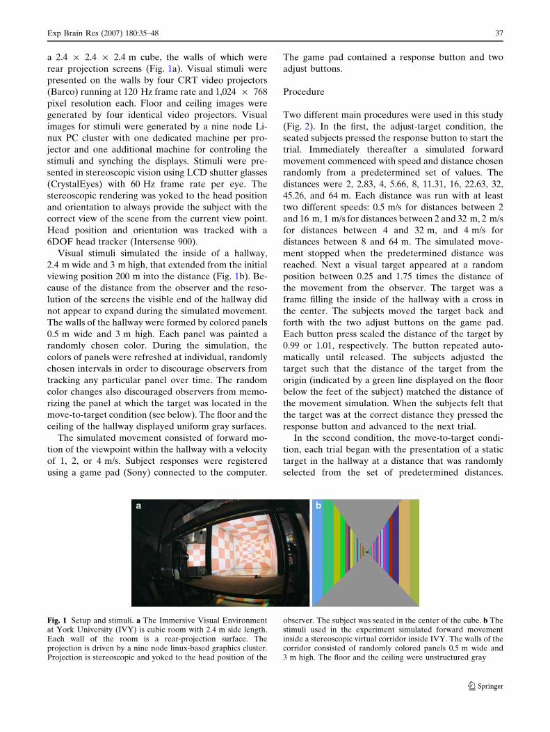
Fig. 1 Setup and stimuli. a The Immersive Visual Environmentat York University (IVY) is cubic room with 2.4 m side length.Each wall of the room is a rear-projection surface. Theprojection is driven by a nine node linux-based graphics cluster.Projection is stereoscopic and yoked to the head position of the

observer. The subject was seated in the center of the cube. b Thestimuli used in the experiment simulated forward movementinside a stereoscopic virtual corridor inside IVY. The walls of thecorridor consisted of randomly colored panels 0.5 m wide and3 m high. The floor and the ceiling were unstructured gray

Exp Brain Res (2007) 180:35–48 37

123

Distances, and speeds for the subsequent movement,

were the same as in the adjust-target condition. When

the subjects pressed the response button, the target was

extinguished and simulated forward movement began

with the randomly chosen speed. The subjects had to

monitor the movement along the hallway and press the

button again as soon as they felt that the position of the

target was reached.

The two conditions were run in blocks with order of

blocks randomized between subjects. Before data col-

lection began, the subjects were given a few practice

trials to familiarize them with the task. No feedback

about performance was given in the practice trials or in

the experimental trials. The order in which the condi-

tions were run was randomized between subjects. To

further reduce the influence of practice effects subjects

usually completed two blocks of each condition. The

second block was run at a later time when other con-

ditions, including further conditions presented below,

were run in-between. In each block, each of the dis-

tance and speed combinations described above was

presented once. The number of trials per block was 32.

For the adjust-target condition, the distace to the

adjusted target was the dependent variable. For the

move-to-target condition, the distance covered during

the movement from start to button press was the

dependent variable.

Results

Adjust-target task

We first tested whether distance and speed of the

simulation influenced the target placement. Because

not all speeds were used with every distance we

grouped conditions into three speed groups for the

analysis. Each speed group covered the range of

distances used with the respective speeds. The three

speed groups were low (0.5 and 1 m/s, distances over

the range of 2–16 m), medium (1 and 2 m/s, distances

over the range of 4–32 m), and high (2 and 4 m/s,

distance over the range of 8–64 m). For the low speed

group, an ANOVA with factors speed and distance

gave a significant influence of distance (F(1,6) = 45.6,

P < 0.001) and a small but significant difference

between speeds (F(1,6) = 20.7, P < 0.001) as well as a

significant interaction (F(1,6) = 2.3, P < 0.05). For the

medium speed group, an ANOVA with factors speed

and distance gave a significant influence of distance

(F(1,6) = 63.4, P < 0.001), no significant difference

between speeds, and no significant interaction. For

the high speed group, an ANOVA with factors speed

and distance gave a significant influence of distance

(F(1,6) = 90.4, P < 0.001), no significant difference

between speeds, and a significant interaction

(F(1,6) = 2.3, P < 0.05). Since speed influenced the

target placement only slightly and only for small

distances we collapsed the data over speeds and

analyzed the dependence of target placement on

distance.

Figure 3a plots the median target placement as a

function of travel distance over subjects. The figure

shows that subjects generally underestimated the dis-

tance of the movement, i.e., placed the target too

near, in the adjust-target condition. For example,

when the distance of the movement was 16 m subjects

on average placed the target at a distance of 12.3 m,

i.e., 3.7 m , or 28%, repectively, too close. The

underestimation was especially pronounced for large

distances, reaching 14 m (22%) for 64 m of move-

ment. For short distances, target placement was closer

to correct. For example, the avearge target placement

for the 4 m movements was 3.83 m, i.e., only 17 cm

(3%) too close.

d

d

“stop”!

Visual target distance

Movement= target distance adjust target distance

Move to target

a

b

Fig. 2 Procedures for Experiment 1. a In the adjust-targetcondition, first a visually simulated forward movement with arandomly chosen distance and speed was presented. Then avisual target appeared at a random position between 0.25 and1.75 times the distance of the movement from the observer. Thesubject adjusted the target such that the distance to the targetmatched the distance of the movement simulation. b In themove-to-target condition, each trial began with the presentationof a static target in the hallway at a random distance. When thesubject pressed a button, the target was extinguished and visuallysimulated forward movement with a randomly chosen speed waspresented. The subject had to monitor the movement along thehallway and stop it by pressing the button again when theposition of the target was reached

38 Exp Brain Res (2007) 180:35–48

123

Experiment 1: move-to-target task

In the move-to-target condition, an ANOVA for the

low speed group with factors speed (0.5 and 1 m/s) and

distance (2–16 m) gave a significant influence of dis-

tance (F(1,6) = 91.4, P < 0.001), no significant differ-

ence between speeds, and no significant interaction.

For the medium speed group, an ANOVA with factors

speed (1 and 2 m/s) and distance (4–32 m) gave a sig-

nificant influence of distance (F(1,6) = 87.0,

P < 0.001), no significant difference between speeds,

and no significant interaction. For the high speed

group, an ANOVA with factors speed (2 and 4 m/s)

and distance (8–64 m) gave a significant influence of

distance (F(1,6) = 90.4, P < 0.001), no significant

difference between speeds, and no significant interac-

tion. We therefore collapsed the data over speeds

again.

Figure 3b shows the median travel distance until

button press as a function of initial target distance in the

move-to-target condition. For large distances, subjects

overestimated the distance of movement, i.e. they pu-

shed the response button too early. For an initial target

in 64 m distance the subjects on average pushed the

button after a movement of 54 m. Thus, a movement of

54 m corresponded to a static target distance of 64 m,

which is an overestimation of the movement distance

by 10 m or 18.5%. For short distances, the responses

were more accurate with a slight tendency to under-

estimate the distance of the movement, i.e., to press the

10 20 30 40 50 60

travel distance

10

20

30

40

50

60

detsujdategrat

ecnatsid

10 20 30 40 50 60

initial target distance

10

20

30

40

50

60

levartecnatsid

a

Adjust-target Move-to-target

c

Perceived distance

10 20 30 40 50 60

actual travel distance

10

20

30

40

50

60

deviecreplevart

ecnatsid

b

Fig. 3 Results of Experiment 1. a Adjusted target distanceversus actual distance of the movement simulation. Data pointsare the medians over ten subjects. Error bars give the inter-quartile range. The dashed line indicates veridical perfomance.The continuous line is the fit by the leaky integration model (seesection ‘‘Leaky-integration model’’). The adjusted target dis-tance is overall smaller than the actual travel distance. Thus, theperceived travel distance underestimates the actual traveldistance. b Travel distance in the move-to-target condition vs.distance to the initially seen static target. The actual traveldistance is overall smaller than the distance required to reach the

initial target. Therefore, the perceived travel distance overesti-mates the actual travel distance. c Data from a and b in a plot ofperceived versus actual travel distance. In the adjust-targetcondition, the perceived distance corresponds to the distance tothe adjusted target. In the move-to-target condition, theperceived distance is given by the initial target, since this is thestatic distance that perceptually corresponded to the distance ofthe movement. Note that the error bars are vertical in thiscondition because the dependent variable, the travel distance tothe target, is on the x-axis

Exp Brain Res (2007) 180:35–48 39

123

button a bit too late. For example, for an initial target

distance of 8 m subjects on average pushed the button

after a movement of 8.7 m, which gives an underesti-

mation of 9%.

Discussion of experiment 1

Although the data in Fig. 3a, b look similar the con-

ditions actually show opposite misestimations. For

distances over about 12 m, there was underestimation

of travel distance in the adjust-target condition and

overestimation of travel distance in the move-to-target

condition. In the adjust-target condition, estimated

travel distance corresponds to the placement of the

target, which was on average too close. For example,

for a travel distance of 11.3 m the median adjusted

target distance was 9.9 m, which corresponds to an

underestimation of about 12%. In the move-to-target

condition, the distance traveled until button press

corresponds to the distance at which subjects felt that

they had travelled as far as the initial target distance.

For example, for an initial distance of 45.26 m the

median travel distance was 34.6 m. Thus, a travel dis-

tance of 34.6 m corresponded to a target distance of

45.26 m: an overestimation by 24%.

To better illustrate this difference, Fig. 3c plots the

perceived distance of the movement as a function of

the actual distance of the motion simulation for both

conditions. In the adjust-target condition, the actual

distance simulated was the distance of the motion

simulation, and the perceived distance was the distance

to the adjusted target. In the move-to-target condition,

the actual distance of the simulated movement was the

distance traveled until button press, and the corre-

sponding perceived distance was the initial target dis-

tance, since this is the static distance that perceptually

corresponded to the distance of the movement. Fig-

ure 3c replots the data to illustrate that perceived dis-

tances are smaller than the actual distance of the

movement in the adjust-target condition but larger in

the move-to-target condition, especially for distances

larger than 12 m.

These results are consistent with earlier work (over

a more restricted range of distances) that showed

underestimation in the adjust-target condition (Frenz

and Lappe 2005) and overestimation for large dis-

tances along with underestimation for small distances

in the move-to-target condition (Redlick et al. 2001;

Frenz and Lappe 2005). The results further show that

these estimation errors occur over large distances and

with identical subjects and identical stimuli. It is

therefore likely that the difference is due to inherent

differences in the tasks. We sought for a coherent

explanation for both effects.

Distance over- or under-estimation in a particular

experimental setting can be explained in many ways.

The combination of underestimation in one task and

overestimation in another, however, restricts the pos-

sibilities.

First, let us look at a candidate explanation that does

not work. The perceived distance to a static visual

target is usually underestimated (Luneburg 1950; Foley

1980; Loomis et al. 1992). This underestimation is even

more pronounced in virtual environments (Knapp and

Loomis 2004; Thompson et al. 2004; Plumert et al.

2005). When we asked subjects to verbally indicate the

distance to the initially presented target in meters we

also found a severe underestimation of the distance

(Fig. 4). Note that interpreting subjects reported dis-

tance in meters is complicated because it involves an

explicit scale. However, as explained below, any

coherent underestimation of static distances could not

explain the misestimation of travel distances we report

which has both over- and underestimation.

Let’s assume that, in the move-to-target trials, the

subjects initially saw the target at a particular distance

and formed a mental representation of the target dis-

tance which, according to the underestimation of static

distances, is less than the true target distance. If the

subjects then used this distance representation during

move-to-target trials, they should have pressed the

button early, because the movement reached the rep-

resented distance earlier than the true distance (note

that this assumes that the estimation of travel distance is

essentially veridical). Thus, an understimation of static

distance may explain the data of the move-to-target

10 20 30 40 50 60

target distance

10

20

30

40

50

60

deviecrepsrete

m

Fig. 4 Underestimation of static distances. The plot shows themedian reported distance to a static target versus the truedistance to the target. The distance to the target is perceptuallyforeshortened

40 Exp Brain Res (2007) 180:35–48

123

trials. It would predict, however, different results in the

adjust target trials. If we again assume that travel dis-

tance estimation is veridical, then, at the end of the

movement in the adjust-target trials the subjects should

have a correct representation of the travel distance. If

the subjects then adjusted the static target to match that

distance representation the target would have been set

further than the value of the distance representation,

because the perceived distance to the target was less

than its actual distance to the target. This would predict

that data in Fig. 3a should be larger than veridical

(above the dashed line) by about the same magnitude as

the data in Fig. 3b is lower than veridical. Clearly, this is

not the case.

The argument works the same way if one begins

with the adjust-target condition and then tries to

predict the data for the move-to-target condition. An

assumed misrepresentation of static distance may ex-

plain the data in one condition but will then fail to

predict the data in the other condition. The combi-

nation of underestimation in one task and overesti-

mation in the other task constrains the possible

explanations.

It is noteworthy that the data in in Fig. 3a, b are

similar, however, in that the amount of over-/under-

estimation increases with increasing travel/target dis-

tance. Moreover, the variance, plotted in Fig. 3 by the

inter-quartile range, also increases with increasing

distance. These observations suggest that the cause of

the misestimation involves some form of decay over

distance.

Leaky-integration model

Path integration is an important concept in distance

estimation from vestibular and proprioceptive signals

(Mittelstaedt and Mittelstaedt 1973, 2001; Maurer and

Seguinot 1995; Loomis et al. 1999). In path integration,

the individual is assumed to track the amout of space

covered by an extended movement—and the direction,

which we do not use here because our movement is

one-directional—by accumulating segments of indi-

vidual movements over the course of the entire

movement. Mathematically this amounts to integrating

position throughout the movement. Misrepresentation

of the length of the entire movement may arise if the

integration of the new position uses a misrepresenta-

tion of the momentary position change (essentially a

gain issue) or if the integration is leaky. We wanted to

explore whether such leaky integration could fit our

data set, including both the adjust-target and move-

to-target conditions.

Leaky integration assumes that a state variable, such

as the current distance from the starting point, is

incremented with each step by the distance of the step

with a gain factor k, but that it is subsequently slightly

reduced in proportion to a leak factor a. Thus, the state

variable is continuously incremented according to the

movement but has a tendency to decay by itself.

In path integration, the integration over the path

segments can be performed in time, i.e., the state var-

iable is updated in successive time intervals, or over

space, i.e., the state variable is updated with every step

taken (Mittelstaedt and Mittelstaedt 1973). For perfect

integration these are equivalent and most models for

path integration integrate the positions over time. If

the integration leaks, however, there is a difference

between integration over time and integration over

space. The former predicts that the state variable de-

cays with time, even when the individual does not

move. The latter predicts that the state variable decays

only when there is movement. Furthermore, integra-

tion over time predicts that the distance estimate, i.e.,

the value of the state variable at the end of the

movement, depends on the movement duration. If the

movement takes longer, there is more decay through

leakage. Hence, movements that cover the same dis-

tance but do so with different speeds are predicted by

such a leaky integrator model to result in different

estimates of path length. This was not the case in our

experiments where speed was found not to be a sig-

nificant factor. We therefore explored a leaky inte-

grator model integrating over space.

The model is explained in detail in the Appendix.

For the adjust-target condition, we assume that the

state variable is the distance from the origin. The state

variable is incremented by an amount proportional to

the length of the step size with a proportionality con-

stant, or gain factor, k. In the mathematical formula-

tion the step size is considered infinitesimal, but

conceptually it can be thought of as having a small but

finite length. Leakage occurs with every spatial step

and is proportional to the current value of the state

variable with a proportionality constant, or leak rate, a.

The model predicts that longer distances lead to more

decay such that the percentage of underestimation in-

creases with the distance of the movement. This is

qualitatively in accordance with the data.

In the move-to-target condition, the task begins with

a given distance that has to be covered with the sub-

sequent movement. We assume that the state variable

is the distance to the target, which has to be nulled by

the movement. The state variable is decremented in

every step proportional to the length of the step size.

The proportionality constant is again k, the same value

Exp Brain Res (2007) 180:35–48 41

123

as used in modeling the adjust-target data. The leakage

occurs with every spatial step and is proportional to the

current value of the state variable according to the leak

rate, a, also the same value as used above. This model

predicts that two processes lead to a reduction of the

perceived distance to the target: the decrement

according to the forward movement and the leakage of

the integrator. Thus, with ongoing movement the dis-

tance to the target becomes overproportionally smaller

because of the leakage, and the point of perceived

distance zero is reached early. Again, this is qualita-

tively consistent with the data.

The appendix details how the point at which the

target is reached is calculated from the initial distance

using the leaky integration model. In order to see how

the model agrees with the data quantitatively we fitted

the model parameters k and a to the data from the two

conditions. The best fit model is generated with

k = 0.98 and a = 0.0076 and is plotted as continuous

lines through the data in Fig. 3.

The leaky integration model explains both under-

estimation in the adjust-target condition and overesti-

mation in the move-to-target condition with the same

set of parameters. This is because the leakage works

towards reducing the current estimate of travel dis-

tance in the adjust-target condition, but works towards

reducing the current estimate of distance to the target

in the move-to-target condition. A similar proposal has

been made by Mittelstaedt and Glasauer (1991), but

for a leaky integrator over time.

The gain factor k describes whether the increment in

each step of the integrator is larger (k > 1) or smaller

(k < 1) than the actual step size. Because the best fitting

k is slightly smaller than one (0.98) the input to the

integrator is slightly smaller than the veridical distance

covered by each step. Thus, the curves in Fig. 3a, b are

both below the line of slope 1. However, for other values

of the parameters, the leaky integration model may yield

other combinations of over- and underestimation. Fig-

ure 5 presents examples of model fits to the data from

three individual subjects to show the variability in re-

sponses and the ability of the model to capture this

variability. The performance of subject JS (k = 0.99 and

a = 0.011) is very similar to the average performance

shown in Fig. 3. Subject LRH (k = 0.79 and a = 0.011)

shows more pronounced underestimation in the adjust-

target condition, and in the move-to-target condition

underestimation for target distances below 30 m and

overestimation for targets beyond 30 m. The model

captures this behavior and thus demonstrates that it can

yield underestmation and overestimation of the trav-

elled distance depending on the target’s distance. Sub-

ject MBC (k = 1.25 and a = 0.015) shows strong

overestimation in the move-to-target condition, and

some overestimation for short distances and underesti-

mation for large distances in the adjust-target condition.

Here, the best fitting gain factor k was larger than one,

indicating that the input to the integrator is larger than

the veridical distance covered by each step.

Experiment 2: updating of target distance

The leaky integration model holds that in the move-to-

target condition the distance to the target decreases

over the course of the movement, because of the

leakage. Thus, if the movement runs only part of the

way the remaining distance to the target should be

overproportionally decreased. To validate the model,

we tested this prediction in an experiment that com-

bined initial vision of the target with later adjustment

of the remaining target distance.

Procedure

The experimental trials in Experiment 2 consisted of

three phases, as shown in Fig. 6, which were all taken

from the experiment described above. First, the se-

ated subject pressed the response button to start the

trial. Upon button press, a static target was presented

in the static hallway at a distance that was randomly

selected from the set of predetermined distances (4,

5.66, 8, 11.31, 16, 22.63, 32, 45.26, and 64 m). When

the subjects pressed the response button again, the

target was extinguished and simulated forward

movement began with the speed and duration ran-

domly chosen from a predetermined set of values.

The speeds: were 1 m/s for distances between 4 and

16 m, 2 m/s for distances between 4 and 64 m, and

4 m/s for distances between 22 and 64 m. The dis-

tance of the simulated movement covered only either

70.7 or 50% of the true distance to the target such

that the movement ended at the next-smaller or the

second-to-next-smaller distance from the original set

of distances. For example, if the initial distance was

16 m, the movement ended after 11.31 or 8 m. The

total number of trials was 36.

The simulated movement stopped when the prede-

termined distance was reached. The subsequent

adjustment procedure now concentrated on the final

target distance, i.e., the remaining part of the distance

from the initial target to the observer (e.g., if the initial

distance were 16 m and the movement covered

11.31 m the final target distance was 4.69 m). The

visual target re-appeared at a random position between

0.25 and 1.75 times the final target distance. The

42 Exp Brain Res (2007) 180:35–48

123

subject adjusted the position of the target such that the

distance of the visible target from the subject (indi-

cated by a green line on the floor below the feet of the

subject) matched that final target position after the

movement simulation, or, in other words, such that the

visible target was at the same place in the hallway as it

was initially.

Results and discussion

From the best fit parameters of the leaky integration

model to the previous adjust-target and move-to-target

conditions one can calculate the prediction for the

perceived final target distances, i.e., the distance that

the observer adjusts. This is given by Eq. 5 in the

Appendix. The prediction and the data from the

experiment are shown in Fig. 7.

The predictions of the leaky integrator model can be

summarized as follows. First, the adjusted target dis-

tance is smaller than the true target distance, because

of the leakage and because the gain is smaller than one.

Second, for longer initial distances and therefore

longer movement distances the undershoot in the ad-

justed target distance becomes progressively larger as

more and more leakage occurs. Because the final target

distance is a constant proportion of the initial distance

Fig. 5 Fits of the leakyintegration model to theresults of Experiment 1 forthree individual subjects.Each data point is the averageof between two and fourtrials, hence no error bars areshown. The individual resultsillustrate the variability inperfomance between the twotask. The model captures thisvariability. The best-fitparameters of the modeldiffer between subjects butare identical for bothconditions for each subject

Exp Brain Res (2007) 180:35–48 43

123

(50 or 70.7%) this predicts that the undershoot should

also increase with increasing final target distance.

Third, for the same final target distance, the adjusted

target distance is smaller in the condition that went

70.7% of the way than in the condition that went 50%

of the way. This is because the former covered a longer

distance and therefore involved more leakage.

All of these predictions are borne out by the data

(Fig. 7). First, the adjusted target distances lie below

the line of slope 1, i.e., they undershoot the true final

target distance. Second, the undershoot becomes pro-

gressively larger with increasing final target distance.

This dependence of the undershoot on final target

distance was significant (F(1,16) = 16.2, P < 0.001,

ANOVA with factors travel percentage (50% or

70.7%) and final target distance). Third, the adjusted

target distances were significantly smaller in the 70.7%

condition than in the 50% condition (F(1,16) = 25.2,

P < 0.001, ANOVA with factors travel percentage and

final target distance). Figure 7 shows that the data

matches the predictions very well in the condition that

went 70.7% of the way but somewhat overreaches the

prediction in the condition that went 50% of the way to

very far targets.

General discussion and conclusions

This study started out from apparent differences in the

ability to gauge distance from optic flow in two dif-

ferent experimental paradigms. Motion based distance

estimates undershot the true distance of a simulated

self motion when the distance from the starting point

had to be indicated (Frenz and Lappe 2005; Lappe

et al. 2005) but overshot the true distance of a simu-

lated self motion when the arrival at a previously

specified location had to be indicated (Redlick et al.

2001; Frenz and Lappe 2005). Comparing both meth-

ods in the same setup and with the same set of subjects

yielded several new findings. First, distances are

underestimated in the adjust-target condition and

overestimated in the move-to-target condition espe-

cially for large movement distances. Second, the

dependence of under-/overestimation on movement

distance is not linear, as earlier results had sug-

gested (Redlick et al. 2001; Frenz and Lappe 2005),

but resembles a logarithmic function. Third, the

Fig. 6 Procedure for Experiment 2. Each trial began with thepresentation of a static target in the hallway at a randomdistance. The subjects estimated and memorized the distance tothe target. When the subject pressed the button, the target wasextinguished and visually simulated forward movement with arandomly chosen speed was presented. The simulated movementstopped after part of the way to the target, either when 50 or

70.7% of the distance to the target was reached. Then the visualtarget re-appeared at a random position between 0.25 and 1.75times the remaining distance from the observer. The subjectadjusted the target such that the distance to the target matchedthe remaining distance, i.e., such that the target appeared to be inthe same spot in the hallway as before

5 10 15 20 25 30

final target distance

5

10

15

20

25

30

detsujdategrat

ecnatsid

Fig. 7 Results of Experiment 2. Adjusted target distance versusactual remaining target distance after the part-way movementsimulation. Data points are the medians over ten subjects. Errorbars give the inter-quartile range. Squares present data from trialsin which the movement covered 70.7% of the initial distance tothe target. Diamonds present data from trials in which themovement covered 50% of the initial distance to the target. Thedashed line indicates veridical perfomance. The continuous linesare the predictions of the leaky integrator model with itsparameters taken from Experiment 1. The adjusted targetdistance is overall smaller than the actual remaining distanceto the target. This underestimation of remaining target distanceis stronger when a longer path had been traversed. These effectsare predicted by the model

44 Exp Brain Res (2007) 180:35–48

123

misestimation occurs even in a fully immersive virtual

environment that contains ample depth cues from

stereo vision and motion parallax from tracked head

movements. Fourth, the misestimation cannot result

solely from a general underestimation of static dis-

tance because this would predict opposite results: if

the static target in the move-to-target condition is

perceived too near to the observer than, the adjusted

target in the adjust-target position should also be

perceived too near to the observer. To indicate the

veridical movement distance the target would then

have to be placed further from the observer so that its

perceived distance matches the true travel distance.

The data show, however, that the target is commonly

placed too near.

Perceived static distance is often underestimated in

virtual reality when compared to distance estimates in

real environments, depending on factors of the display

(Knapp and Loomis 2004; Thompson et al. 2004;

Plumert et al. 2005). Our own measurement of per-

ceived distance to the static target also suggests

underestimation (Fig. 4) that is stronger than that

typically found in real world measurements (Luneburg

1950; Foley 1980; Loomis et al. 1992). It may be that

our distance misestimates from motion also exaggerate

the errors that occur in equivalent real life situations.

However, the use of virtual technology is the only way

to study the usage of pure visual signals during self-

motion without vestibular or proprioceptive inputs.

Sun et al., (2004) studied distance perception to static

targets in real world experiments with methods very

similar to ours. They also compared distance indication

in a condition that involved walking to a remembered

stationary target with distance indication in a condition

in which a target had to be adjusted to reflect the dis-

tance of a prior walk. Error analysis suggested a

common representation of walking distance in the full

cue situation (vision, proprioceptive, and vestibular

information present) but a dependence on condition

when only proprioceptive and vestibular information

were available. It is difficult to compare this directly to

our results, however, because their conditions always

included proprioception and vestibular cues.

Based on the differences in estimation of travel

distance in the two conditions we propose a leaky

integration model. In this model the parameter nec-

essary for the completion of the experimental task is

continuously updated with new movement informa-

tion. The task-relevant parameter is the distance from

the origin in the adjust-target condition and the dis-

tance to the target in the move-to-target condition. The

continuous updating follows the same rules and

parameters in both conditions such that the distance

from the origin is incremented with a particular gain

for every instantaneous movement, and the distance to

the target is decremented according to the same gain

value. The integration is assumed to be leaky with the

same leakage factor in both conditions. Because of the

leak, the distance from the start point in the one con-

dition and the distance to the target in the other con-

dition are reduced over the course of the movement.

This results in underestimation of the travel distance

from the origin in the adjust-target task and at the

same time in an overestimation of the distance covered

in approaching the target in the move-to-target task.

Our model integrates over space. Integrating travel

distance over time is not consistent with the data, since

it would predict a dependence on duration of the

movement, and hence speed, which was not observed.

Integrating in spatial coordinates is interesting because

it predicts that leakage should only occur during

movement. If leaky integration occurred over time, on

the other hand, leakage should occur as time pro-

gresses even if the observer remains stationary. Thus,

because of integration over space the integration is

automatically yoked to the observer movement. Inte-

gration over space predicts that the amount of leakage

increases with the distance of the movement (con-

firmed in Experiment 2).

In order to allow integration to occur over space,

the visual system must convert the visual motion

signal from every—theoretically infinitesimal—spatial

step to the momentary distance gain by that step.

This involves an additional integration process, that

of motion to position, before the signal can be used

in the distance integrator. The effectiveness of such

integration is captured in the model by the gain

factor k. If k = 1, each infinitesimal step is converted

accurately into the corresponding distance covered

during the infinitesimal movement. Our observation

that k is on average slightly smaller than one suggests

that the transformation from visual motion to dis-

tance slightly underestimates the instantaneous travel

distance.

Our mathematical model assumes an infinitesimal

step size but it may be that the step size used by

human subjects is finite such that the first integration

is performed over a particular step distance and the

result is added to the state variable in an iterative

manner. Our data give no indication of this, but it

may be interesting for further study. Moreover, the

integration gain from motion to momentary distance

may depend on the availablity of visual depth cues

such as stereo or perspective foreshortening, and may

in more natural situations also access proprioceptive

or vestibular information about instantaneous velocity

Exp Brain Res (2007) 180:35–48 45

123

and movement distance. It would be interesting to

investigate whether the availability of such cues

modulates the value of the gain and whether or not

this affects the integration constant a.

The underestimation of static distance that we ob-

served cannot explain the difference between the dis-

tance estimates in the two conditions. However, static

distance estimates are required to fulfill the task in

both conditions. It may thus be that the foreshortening

of static distances also modulates the task perfor-

mance. We explored including the static distance

foreshortening in the model by an additional trans-

formation step in which perceived static distance was

calculated from true static distances according to Fig. 4

and vice versa. In this variant of the model, initial

target distance in the move-to-target condition was first

converted into a perceived target distance and the

subsequent integration of movement distance was

performed until the perceived distance was reached. In

the adjust target condition, the final estimate of

movement distance was considered to be a perceived

distance and this was then converted into a true dis-

tance. The best fit by this model was considerably

worse than the fit by the original model. We therefore

concluded that the underestimation of static distances

did not contribute to the estimation of travel distance

from visual motion.

To conclude, our results show that humans are

capable of estimating travel distance from visual mo-

tion alone, by using an integration process, but one that

leaks over the spatial extent of the movement. Our

model suggest that the task to be performed (estimat-

ing the cumulative distance from start or estimating the

remaining distance to goal) determines the variable to

be integrated over the movement, but that the inte-

gration process itself is the same.

Acknowledgments M.L. is supported by the German ScienceFoundation DFG LA-952/2 and LA-952/3, the German FederalMinistry of Education and Research BioFuture Prize, and theEC Project Drivsco. L.R.H. and M.J. are supported by theNational Sciences and Engineering Research Council of Canada.

Appendix

In the adjust-target condition, the subjects first expe-

rience the visual motion for a particular travel distance.

Thereafter the subjects adjust the target such that its

distance from the observer matches the travel distance.

We assume that the subjects monitor their current

perceived position p(x) from the starting position p(0)

= 0 during the movement, and adjust the target such

that its distance is the value of p at the end of the

movement. The current position is updated during the

movement according to the following leaky integrator

differential equation:

dp

dx¼ �apþ k; ð1Þ

where dx is the change of position of the subject along

the trajectory of the movement, a is the rate of decay of

the integrator, and k is the gain of the sensory (visual)

input. If k = 1 the visual motion is transformed per-

fectly into the instantaneous travel distance. In this

equation, in each step dx, the state variable p is re-

duced proportional to its current value (due to the

leak) and incremented by the distance given by the

gain k of the step.

The general solution to this differential equation is

pðxÞ ¼ e�axþb þ k

a:

The value of b is constrained by the starting position of

the integrator, p(0) = 0. Therefore,

eb þ k

a¼ 0;

or

b ¼ ln � k

a

� �:

Thus the solution to Eq. 1 is given by

pðxÞ ¼ e�axþlnð�kaÞ þ k

a¼ k

að1� e�axÞ: ð2Þ

In the move-to-target condition, the subjects first see

the target at a particular distance. Then, the target is

extinguished and the subjects move towards the

target. The subjects stop the movement by pressing

a button when they feel that the target is reached. We

assume that the subjects monitor the current

perceived distance D(x) to the target during the

movement and press the button when this distance

becomes zero. We denote the initial distance to the

target by D(0) = D0 The current distance is updated

during the movement according to the following

differential equation:

dD

dx¼ �aD� k: ð3Þ

This is similar to to Eq. 1, but now the state variable is

the distance to the target rather than the perceived

46 Exp Brain Res (2007) 180:35–48

123

position along the trajectory, and this state variable is

decremented over the course of the movement

according to –k.

The general solution to this differential equation is

DðxÞ ¼ e�axþb � k

a: ð4Þ

Again, the value of b is constrained by the starting

value of the integrator. This is now D(x = 0) = D0.

Therefore,

eb � k

a¼ D0;

and

b ¼ ln D0 þk

a

� �:

Thus the solution to Eq. 4 is

DðxÞ ¼ e�axþlnðD0þkaÞ � k

a¼ D0e�ax � k

að1� e�axÞ: ð5Þ

Equation 5 gives the current distance to the target as a

function of true position x along the movement

trajectory. To calculate the position at which the

subject presses the putton we have to find the

position phit at which the D(x) becomes zero:

DðphitÞ ¼ 0:

From

e�aphitþlnðD0þkaÞ � k

a¼ 0

we find

�aphit þ ln D0 þk

a

� �¼ ln

k

a

� �;

and finally

phitðD0Þ ¼1

aln D0 þ

k

a

� �� ln

k

a

� �� �

¼ 1

aln

k

a

� �½lnðD0 � 1Þ�:

ð6Þ

Equations 2 and 6 are used fit the data from the adjust-

target and the move-to-target conditions, respectively,

with a and k as parameters. The predictions for the

part-of-the-way condition is then derived from using

the best-fit parameters a and k in Eq. 5.

References

Bremmer F, Lappe M (1999) The use of optical velocities fordistance discrimination and reproduction during visuallysimulated self-motion. Exp Brain Res 127:33–42

Etienne AS, Maurer R, Seguinot V (1999) Path integration inmammals and its interaction with visual landmarks. J ExpBiol 199:201–209

Foley JM (1980) Binocular distance perception. Psychol Rev87:411–434

Frenz H, Lappe M (2005) Absolute travel distances from opticflow. Vis Res 45:1679–1692

Frenz H, Bremmer F, Lappe M (2003) Discrimination of traveldistances from ‘situated’ optic flow. Vis Res 43:2173–2183

Gillner S, Mallot HA (1998) Navigation and acquisition ofspatial knowledge in a virtual maze. J Cogn Neurosci10:445–463

Judd SPD, Collett TS (1998) Multiple stored views and landmarkguidance in ants. Nature 392:710–714

Knapp JM, Loomis JM (2004) Limited field of view of head-mounted displays is not the cause of distance underestima-tion in virtual environments. Presence 13(5):572–577

Lappe M, Frenz H, Buhrmann T, Kolesnik M (2005) Virtualodometry from visual flow. In: Rogowitz BE, Pappas TN,Daly SJ (eds.) Proceedings of SPIE/IS&T ConferenceHuman Vision and Electr. Imag. X, SPIE, vol 5666, pp493–502

Loomis JM, Da Silva JA, Fujita N, Fukusima SS (1992) Visualspace perception and visually directed action. J Exp PsycholHum Perc Perform 18:906–921

Loomis JM, Klatzky RL, Golledge RG, Cicinelli JG, PellegrinoJW, Fry PA (1993) Nonvisual navigation by blind andsighted: assessment of path integration ability. J Exp PsychGen 122:73–91

Loomis JM, Klatzky RL, Golledge RG, Philbeck JW (1999)Human navigation by path integration. In: Golledge RG(ed) Wayfinding: Cognitive mapping and other spatialprocesses. Johns Hopkins, Baltimore, pp 125–151

Luneburg RK (1950) The metric of binocular visual space. OptSoc Am 40:627–642

Maurer R, Seguinot V (1995) What is modelling for? A criticalreview of the models of path integration. J Theor Biol175:457–475

Mittelstaedt ML, Glasauer S (1991) Idiothetic navigation ingerbils and humans. Zool Jb Physiol 95:427–435

Mittelstaedt H, Mittelstaedt ML (1973) Mechanismen derOrientierung ohne richtende Außenreize. Fort Zool 21:46–58

Mittelstaedt ML, Mittelstaedt H (1980) Homing by pathintegration in a mammal. Naturwissenschaften 67:566–567

Mittelstaedt M, Mittelstaedt H (2001) Ideothetic navigation inhumans: estimation of path length. Exp Brain Res 139:318–332

Peruch P, May M, Wartenberg F (1997) Homing in virtualenvironments: Effects of field of view and path layout.Perception 26:301–311

Plumert JM, Kearney JK, Cremer JF, Recker K (2005) Distanceperception in real and virtual environments. ACM TransAppl Percept 2(3):216–233

Redlick FP, Jenkin M, Harris LR (2001) Humans can use opticflow to estimate distance of travel. Vis Res 41:213 – 219

Riecke BE, van Veen HAHC, Bulthoff HH (2002) Visualhoming is possible without landmarks: a path integrationstudy in virtual reality. Presence 11:443–473

Exp Brain Res (2007) 180:35–48 47

123

Robinson M, Laurence J, Hogue A, Zacher JE, German A,Jenkin M (2002) Ivy: basic design and construction details.In: Proceedings of ICAT, Tokyo

Sun H-J, Campos JL, Young M, Chan GSW (2004) Thecontributions of static visual cues, nonvisual cues, and opticflow in distance estimation. Perception 33:49–65

Thompson WB, Willemsen P, Gooch AA, Creem-Regehr SH,Loomis JM, Beall AC (2004) Does the quality of thecomputer graphics matter when judging distances in visuallyimmersive environments? Presence 13(5):560–571

48 Exp Brain Res (2007) 180:35–48

123