LAND USE CLASSIFICATION FROM VHR AERIAL IMAGES USING INVARIANT COLOUR COMPONENTS AND TEXTURE

A. Movia a, A.Beinat a, T. Sandri

a Polytechnic Department of Engineering and Architecture, via delle Scienze 206, University of Udine, Italy movia.alessia@spes.uniud.it

COMMISSION VII/4

KEY WORDS: High resolution colour images, texture, classification, invariant colour spaces, aerial images ABSTRACT: Very high resolution (VHR) aerial images can provide detailed analysis about landscape and environment; nowadays, thanks to the rapid growing airborne data acquisition technology an increasing number of high resolution datasets are freely available. In a VHR image the essential information is contained in the red-green-blue colour components (RGB) and in the texture, therefore a preliminary step in image analysis concerns the classification in order to detect pixels having similar characteristics and to group them in distinct classes. Common land use classification approaches use colour at a first stage, followed by texture analysis, particularly for the evaluation of landscape patterns. Unfortunately RGB-based classifications are significantly influenced by image setting, as contrast, saturation, and brightness, and by the presence of shadows in the scene. The classification methods analysed in this work aim to mitigate these effects. The procedures developed considered the use of invariant colour components, image resampling, and the evaluation of a RGB texture parameter for various increasing sizes of a structuring element. To identify the most efficient solution, the classification vectors obtained were then processed by a K-means unsupervised classifier using different metrics, and the results were compared with respect to corresponding user supervised classifications. The experiments performed and discussed in the paper let us evaluate the effective contribution of texture information, and compare the most suitable vector components and metrics for automatic classification of very high resolution RGB aerial images.

1.1.1.1. INTRODUCTION

Large datasets of aerial imagery exist in different government institutions, such as national land, urban planning, and construction departments (Lv et al., 2010). Commonly, the spatial resolution can be high or even very high, but the spectral resolution is often limited to RGB, and there is a general lack of the near-infrared bands (Laliberte and Rango, 2009). In the classification of RGB images, without the fundamental contribution of NIR and other bands, the quality of the process is variably influenced by different factors such as subject, illumination conditions, spatial resolution, vector components and metrics used to define the various clusters. In order to classify an image, it is common to use methods based on statistical analysis of pixels: this approach has demonstrated to have good performances only when used to classify images with large pixel size (Wang et al., 2004). High spatial resolution digital aerial imagery, with a pixel size less than one meter, is an underexplored field in which the classification process can be complicated by the spectral variability within a particular class due to the very small pixel size (Aguera et al., 2008), especially in the case of urban areas (Kiema, 2002). The urban environment in particular represents one of the most challenging problems for remote sensing analysis as a consequence of high spatial difference and spectral variance of the surface materials (Herold et al., 2003). This question can be overcome with different techniques that take into account two fundamental image characteristics: colour (spectral information) and texture (Haralick et al., 1973). Colour has high discriminative power, and in many cases objects can be well recognized merely by this characteristic (Swain and Ballard, 1991; Burghouts and

Geusebroek, 2009). Texture information can be used for directly classify images or as additional band in the clustering process; in the last case, classification accuracies are generally improved (Wang et al., 2004; Puissant et al., 2005; Rao et al., 2002). Further, texture estimation is important because provides information about spatial and structural arrangement of objects, thanks to the strong correspondence between them and their pattern (Tso and Mather, 2001; Permuter et al., 2006). Even though colour is the most appealing feature, it is also the most vulnerable indexing parameter, since it strongly depends on image lighting conditions, pose and sensor characteristics. This problem affects also texture evaluation, and there is no valid model able to provide illumination invariant entities (Hanbury et al., 2005). Few applications of RGB classification for land use setimation are present in literature. Among these, Chust et al., (2008) used an initial RGB supervised classification as reference, and compared it with those automatically obtained adding further information – NIR, DTM, aspect, slope – reaching a mean accuracy of 73.2% and 75.1% on the two test areas considered. Lv et al. (2010) developed a method to carry out land cover classifications that depend only on RGB bands reaching high values of accuracy. They observed that in order to extract building information, it is necessary to include spectral and texture features. This work provides an experimental assessment of the benefits derived from converting the RGB colour components into invariant ones, in order to remove or at least mitigate the classification biases caused by the varying scene illumination conditions, that produce different RGB spectral signatures for identical image objects. Further, the tests carried out aim to evaluate the actual improvements in high resolution colour image classification provided by textural information and spatial resolution resampling.

The International Archives of the Photogrammetry, Remote Sensing and Spatial Information Sciences, Volume XLI-B7, 2016 XXIII ISPRS Congress, 12–19 July 2016, Prague, Czech Republic

This contribution has been peer-reviewed. doi:10.5194/isprsarchives-XLI-B7-311-2016

311

1.1 Invariant image features

In image processing, various colour systems related to RGB are in use today: among their characteristics, for the purpose of image classification, an important colour property is the invariance. A colour invariant system contains models which are more or less insensitive to the varying imaging conditions such as variations in illumination and object pose (Gevers, 1998). Colour invariants can be obtained by constructing a colour ratio model to remove the effects of perspective, light direction, illumination, reflected light intensity, and other factors. HSV, C1C2C3, l1l2l3, CIE-Lab and CIE-Luv are some invariant colour models described in literature and briefly recalled below (e.g. Gevers and Smeulders, 1999; Geusebroek et al., 2001). In addition, other techniques as the SIFT model and image stretch decorrelation can be considered for the same purposes. Thanks to these characteristics all these methods appear suitable to improve the classification accuracy, and to mitigate the distortions of RGB caused by different light conditions. 1.1.1 HSV colour model HSV is an approximately perceptually uniform colour space that provides an intuitive representation of colours and simulates the way humans perceive and manipulate them. Hue (H) represents the dominant spectral component, and is commonly used in tracking applications where some degree of illumination changes are expected. The hue component doesn’t contain intensity information, and therefore it is invariant to intensity changes in illumination, however, it is sensitive to light colour changes. Saturation (S) is an expression of the relative purity, that is the degree to which a pure colour is diluted by adding white. Finally, the value (V) corresponds to the colour brightness. In this way, the luminous component (V) is decoupled from the colour-carrying information (H and S). HSV can be obtained from RGB through a nonlinear invertible transformation. After rescaling the RGB coordinates to the range [0,1] by dividing them by their maximum theoretical value (e.g. 255 for an 8 bit colour band), H, S, and V are estimated as follows:

( )max max , ,C R G B=

( )min min , ,C R G B=

max minC C C∆ = −

max

max

max

0 if 0 or 0

if6

1if

6 32

if 6 3

1 if 1

C H

G BC R

CB R

H C GC

R GC B

CH

∆ = < − = ∆ −= + =

∆ − + = ∆

>

max

0 if 0

otherwise

C

S C

C

∆ == ∆

maxV C=

1.1.2 C1C2C3 and l1l2l3 colour model C1C2C3 and l1l2l3 represent colour models that are theoretically insensitive to viewing direction, surface orientation, illumination direction and intensity. The C1, C2 and C3 band components can be calculated from R, G, B by the following formulas:

{ }1 arctanmax ,

RC

G B

=

{ }2 arctanmax ,

GC

R B

=

{ }3 arctanmax ,

BC

R G

=

The following equations provide the transformation from R, G, B to l1, l2, l3, that forms a set of normalized colour differences:

( )( ) ( ) ( )

2

1 2 2 2

R Gl

R G R B G B

−=

− + − + −

( )( ) ( ) ( )

2

2 2 2 2

R Bl

R G R B G B

−=

− + − + −

( )( ) ( ) ( )

2

3 2 2 2

G Bl

R G R B G B

−=

− + − + −

where R, G, B are the Red, Green, and Blue band component values respectively (Gevers and Smeulders, 1999). 1.1.3 CIE-Lab and CIE-Luv L*a*b* and L*u*v* are two perceptual uniform colour spaces, specified by the International Commission on Illumination (CIE), that are considered device independent. There are no simple and univocal formulas to convert from RGB to L*a*b* and L*u*v*, since RGB is device dependent; in any case, for classification purposes, a suitable transformation can be obtained converting RGB to CIE-XYZ, and then deriving L*a*b* and L*u*v* under standard conditions. To this aim, at first R,G,B coordinates are rescaled to the range [0,1] by dividing them by their maximum theoretical value, then the X, Y, Z tristimulus values are evaluated as follows:

( )( )( )

0.4124 0.3576 0.1805

0.2126 0.7152 0.0722

0.0193 0.1192 0.9505

X f R

Y f G

Z f B

= ⋅

where:

( )

1250.055

100 if 0.040451.055: , ,

100 otherwise12.92

tt

f t R G Bt

+ ⋅ > = =

⋅

The International Archives of the Photogrammetry, Remote Sensing and Spatial Information Sciences, Volume XLI-B7, 2016 XXIII ISPRS Congress, 12–19 July 2016, Prague, Czech Republic

This contribution has been peer-reviewed. doi:10.5194/isprsarchives-XLI-B7-311-2016

312

L*a*b* are consequently defined as:

* 116 16n

YL f

Y

= ⋅ −

* 500n n

X Ya f f

X Y

= −

* 200n n

Y Zb f f

Y Z

= −

where:

13 if 0.008856

: , , 841 4otherwise

108 29n n n

t tX Y Zf t

X Y Z t

>

= = ⋅ +

and

95.047 100.000 108.883n n nX Y Z= = =

assuming standard open air illumination conditions. Regarding L*u*v*, the new components u* and v* are obtained as:

L* has same meaning and formulation as in L*a*b*

( ) 4

15 3

Xf u

X Y Z=

+ +

( ) 4

15 3n

nn n n

Xf u

X Y Z=

+ +

( ) 9

15 3

Yf v

X Y Z=

+ +

( ) 9

15 3n

nn n n

Yf v

X Y Z=

+ +

( ) ( )( )* *13 nu L f u f u= ⋅ ⋅ −

( ) ( )( )* *13 nv L f v f v= ⋅ ⋅ −

assuming again standard conditions as above. 1.1.4 SIFT colour model An RGB histogram is not invariant to changes in lighting conditions, however, by normalizing the pixel value distributions, scale invariance and shift invariance are achieved with respect to light intensity. Because each band is normalized independently, the descriptor is also normalized against changes in light colour and arbitrary offsets. SIFT descriptors are computed for every RGB band independently as follow:

'

'

'

R

R

G

G

B

B

R

RG

G

BB

µσ

µσ

µσ

− − =

−

with µ the mean and σ the standard deviation of the distribution of the respective colour bands computed over the area under consideration. 1.1.5 Decorrelation Stretching This colour transformation is used for enhancing the colour differences in images with high internal band correlation, as evident in many RGB ones. Decorrelation makes possible to distinguish picture details that otherwise are not so immediately visible. The specificity of the model is the following pointwise linear transformation:

target( )Tt c= − +y S R S R x μ μ

where: x = input RGB colour pixel vector y = output decorrelated RGB colour pixel vector µ = input dataset mean R = rotation matrix Sc = scaling matrix (diagonal) St = stretching matrix µtarget = backprojected data shift. Refer to Gillespie et al. (1986) for complete description. Figure 1 shows some histogram examples representing transformations from RGB to invariant colour components: worth of note is the lack of correlation existing among the various colour spaces. In the graphs, for better comparison with the original RGB, the various component values have been rescaled to [0 255].

RGB

C1C2C3

L*u*v*

Figure 1: Examples of histograms representing transformations from RGB to invariant colour components.

The International Archives of the Photogrammetry, Remote Sensing and Spatial Information Sciences, Volume XLI-B7, 2016 XXIII ISPRS Congress, 12–19 July 2016, Prague, Czech Republic

This contribution has been peer-reviewed. doi:10.5194/isprsarchives-XLI-B7-311-2016

313

2.2.2.2. EXPERIMENTS

The experimental assessments have been carried out on two image pairs of two suburban environments, acquired respectively in summer 2008 and in winter 2011, at the same resolution (9 cm) (Figure 2).

Figure 2: Image pairs employed for the experiment of two suburban areas at 9 cm resolution: on the left, pictures 1_2008 and 2_2008 taken in summer 2008, while on the right, the corresponding 1_2011 and 2_2011, acquired in winter 2011, showing various long shadows.

The four original images have been resampled, by the median method, producing four additional pictures with 27 cm pixel size, and further four images at 45 cm resolution. The 12 samples thus obtained formed the dataset employed to investigate the benefits of different invariant colour models, together with the role played by pixel size and scene illumination. In the first step, in order to set a reference for the following evaluations, a thorough supervised classification of each of the 12 RGB colour images has been carried out: the results obtained were assumed to represent the truth. The classes considered were: vegetation, urban areas, streets, and shadows. The 12 RGB images were then converted in their corresponding HSV, l1l2l3, C1C2C3 invariant colour components, and in CIE-Luv and CIE-Lab colour spaces; in addition, a SIFT transformation and a stretch decorrelation of the RGB bands was also performed. Each different image thus obtained was classified with K-means unsupervised method, applying in many cases, for further comparison, two possible metrics: Euclidean and cosine distance.

To analyse the effects of texture information in the classification, a further component representing object image texture was considered in some cases, and joined to the clustering vectors: this parameter was the mean RGB component value computed by a structuring element of size 3x3 or 9x9. In this way, varying the vector composition of the test images, 228 independent K-means classifications have been produced, and individually compared with the corresponding reference ones obtained via the supervised approach (Figure 3 and 4). All the various steps of the computations have been performed by custom-made Matlab scripts, taking advantage of built-in high level functions only when necessary (K-means classification and stretch decorrelation).

3.3.3.3. RESULTS AND DISCUSSION

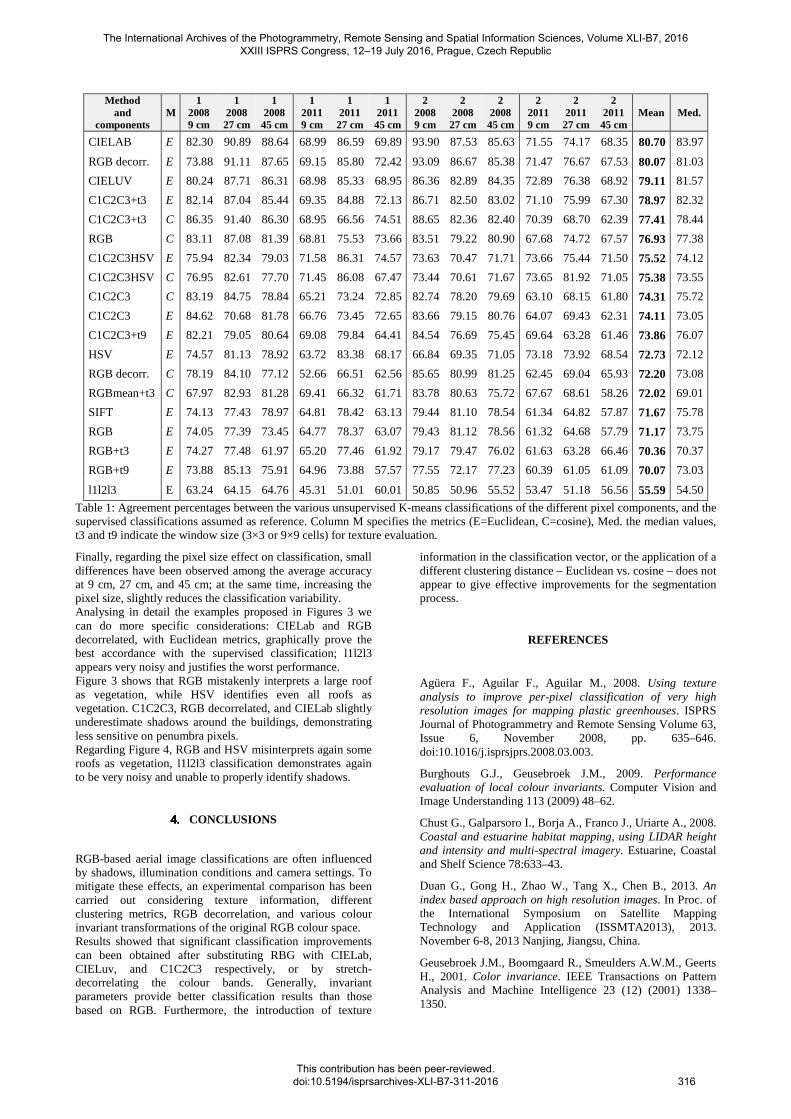
Table 1 collects the percentages of agreement between the various unsupervised K-means classifications of the different pixel components, and the user supervised classifications of the same RGB images, assumed to represent the truth. Column 1 specifies the composition of the classification vector employed, column 2 shows the metric used, and the following twelve columns list the results of the various experiments. The rows are ordered considering the global average agreement obtained in the various tests, and secondly their median value. Following this criterion a significant outcome emerges: classifications exploiting invariant components are generally superior than those based on RGB and texture. Excluding the evident worst case represented by l1l2l3, RGB based methods generally produce average agreements around 71%, while the best three invariant based solutions are very close to 80% and over. Going in detail, must be noted that, starting from the same information, represented by the original RGB image, very different agreements – from 45.3% to 93.9% – can be produced just selecting a specific colour invariant or by stretch decorrelating the colour bands. The minimal variation – from to 57.6% to 74.6% – has been obtained in image 1_2011 at 45 cm, while the maximal one – from 50.9% to 93.9% – has been observed in image 2_2008 at 9 cm. The metric employed appears to be effective only in case of RGB, where substituting Euclidean with cosine distance improves the average agreement of 5 6%. In the other cases the metrics role is very variable. RGB texture information does not seem to provide significant improvements since it produces contrasting results: in the case of RGB, introducing texture 3x3 and 9x9 slightly worsen the outcomes, while in the case of C1C2C3 we observe a significant gain with texture 3x3, and a small loss with texture 9x9. Observing the highest classification results for the various images, they show that L*a*b* performed five times over twelve as the best classifier vector, as in 2008 imagery, but also C1C2C3 based methods achieved similar results, particularly in 2011 images. This can be explained by the fact that 2011 images contain a larger amount of shadows than the corresponding 2008 ones, and the component C3 is particularly suited to detect them, as reported in shadow detection literature (Duan et al., 2013; Movia et al., 2015). In any case, also when CIE-Lab, RGB decorr., and CIE-Luv were not the best ones in the tests, their average distance from them ranges only from 2.1% to 3.7%.

The International Archives of the Photogrammetry, Remote Sensing and Spatial Information Sciences, Volume XLI-B7, 2016 XXIII ISPRS Congress, 12–19 July 2016, Prague, Czech Republic

This contribution has been peer-reviewed. doi:10.5194/isprsarchives-XLI-B7-311-2016

314

*** Supervised(E) ***

RGB(E)

RGB stretch decorrelated(E)

C1C2C3(E)

l1l2l3(E)

HSV(E)

CIELUV(E)

CIELAB(E)

Figure 3: Examples of K-Means classifications of Image 2_2008 at 27 cm with different vector components: blue represents urban areas, cyan identifies streets and bare soil, brown vegetation and yellow shadows. (E) indicates to Euclidean distance.

*** Supervised(E) ***

RGB(E)

RGB stretch decorrelated(E)

C1C2C3(E)

l1l2l3(E)

HSV(E)

CIELUV(E)

CIELAB(E)

Figure 4: Examples of K-Means classifications of Image 1_2011 at 27 cm with different vector components: here blue represents urban areas, cyan identifies streets, yellow vegetation, and brown shadows. (E) indicates Euclidean distance.

The International Archives of the Photogrammetry, Remote Sensing and Spatial Information Sciences, Volume XLI-B7, 2016 XXIII ISPRS Congress, 12–19 July 2016, Prague, Czech Republic

This contribution has been peer-reviewed. doi:10.5194/isprsarchives-XLI-B7-311-2016

315

Method and

components

M

1 2008 9 cm

1 2008 27 cm

1 2008 45 cm

1 2011 9 cm

1 2011 27 cm

1 2011 45 cm

2 2008 9 cm

2 2008 27 cm

2 2008 45 cm

2 2011 9 cm

2 2011 27 cm

2 2011 45 cm

Mean

Med.

CIELAB E 82.30 90.89 88.64 68.99 86.59 69.89 93.90 87.53 85.63 71.55 74.17 68.35 80.70 83.97

RGB decorr. E 73.88 91.11 87.65 69.15 85.80 72.42 93.09 86.67 85.38 71.47 76.67 67.53 80.07 81.03

CIELUV E 80.24 87.71 86.31 68.98 85.33 68.95 86.36 82.89 84.35 72.89 76.38 68.92 79.11 81.57

C1C2C3+t3 E 82.14 87.04 85.44 69.35 84.88 72.13 86.71 82.50 83.02 71.10 75.99 67.30 78.97 82.32

C1C2C3+t3 C 86.35 91.40 86.30 68.95 66.56 74.51 88.65 82.36 82.40 70.39 68.70 62.39 77.41 78.44

RGB C 83.11 87.08 81.39 68.81 75.53 73.66 83.51 79.22 80.90 67.68 74.72 67.57 76.93 77.38

C1C2C3HSV E 75.94 82.34 79.03 71.58 86.31 74.57 73.63 70.47 71.71 73.66 75.44 71.50 75.52 74.12

C1C2C3HSV C 76.95 82.61 77.70 71.45 86.08 67.47 73.44 70.61 71.67 73.65 81.92 71.05 75.38 73.55

C1C2C3 C 83.19 84.75 78.84 65.21 73.24 72.85 82.74 78.20 79.69 63.10 68.15 61.80 74.31 75.72

C1C2C3 E 84.62 70.68 81.78 66.76 73.45 72.65 83.66 79.15 80.76 64.07 69.43 62.31 74.11 73.05

C1C2C3+t9 E 82.21 79.05 80.64 69.08 79.84 64.41 84.54 76.69 75.45 69.64 63.28 61.46 73.86 76.07

HSV E 74.57 81.13 78.92 63.72 83.38 68.17 66.84 69.35 71.05 73.18 73.92 68.54 72.73 72.12

RGB decorr. C 78.19 84.10 77.12 52.66 66.51 62.56 85.65 80.99 81.25 62.45 69.04 65.93 72.20 73.08

RGBmean+t3 C 67.97 82.93 81.28 69.41 66.32 61.71 83.78 80.63 75.72 67.67 68.61 58.26 72.02 69.01

SIFT E 74.13 77.43 78.97 64.81 78.42 63.13 79.44 81.10 78.54 61.34 64.82 57.87 71.67 75.78

RGB E 74.05 77.39 73.45 64.77 78.37 63.07 79.43 81.12 78.56 61.32 64.68 57.79 71.17 73.75

RGB+t3 E 74.27 77.48 61.97 65.20 77.46 61.92 79.17 79.47 76.02 61.63 63.28 66.46 70.36 70.37

RGB+t9 E 73.88 85.13 75.91 64.96 73.88 57.57 77.55 72.17 77.23 60.39 61.05 61.09 70.07 73.03

l1l2l3 E 63.24 64.15 64.76 45.31 51.01 60.01 50.85 50.96 55.52 53.47 51.18 56.56 55.59 54.50

Table 1: Agreement percentages between the various unsupervised K-means classifications of the different pixel components, and the supervised classifications assumed as reference. Column M specifies the metrics (E=Euclidean, C=cosine), Med. the median values, t3 and t9 indicate the window size (3×3 or 9×9 cells) for texture evaluation.

Finally, regarding the pixel size effect on classification, small differences have been observed among the average accuracy at 9 cm, 27 cm, and 45 cm; at the same time, increasing the pixel size, slightly reduces the classification variability. Analysing in detail the examples proposed in Figures 3 we can do more specific considerations: CIELab and RGB decorrelated, with Euclidean metrics, graphically prove the best accordance with the supervised classification; l1l2l3 appears very noisy and justifies the worst performance. Figure 3 shows that RGB mistakenly interprets a large roof as vegetation, while HSV identifies even all roofs as vegetation. C1C2C3, RGB decorrelated, and CIELab slightly underestimate shadows around the buildings, demonstrating less sensitive on penumbra pixels. Regarding Figure 4, RGB and HSV misinterprets again some roofs as vegetation, l1l2l3 classification demonstrates again to be very noisy and unable to properly identify shadows.

4.4.4.4. CONCLUSIONS

RGB-based aerial image classifications are often influenced by shadows, illumination conditions and camera settings. To mitigate these effects, an experimental comparison has been carried out considering texture information, different clustering metrics, RGB decorrelation, and various colour invariant transformations of the original RGB colour space. Results showed that significant classification improvements can been obtained after substituting RBG with CIELab, CIELuv, and C1C2C3 respectively, or by stretch-decorrelating the colour bands. Generally, invariant parameters provide better classification results than those based on RGB. Furthermore, the introduction of texture

information in the classification vector, or the application of a different clustering distance – Euclidean vs. cosine – does not appear to give effective improvements for the segmentation process.

REFERENCES

Agüera F., Aguilar F., Aguilar M., 2008. Using texture analysis to improve per-pixel classification of very high resolution images for mapping plastic greenhouses. ISPRS Journal of Photogrammetry and Remote Sensing Volume 63, Issue 6, November 2008, pp. 635–646. doi:10.1016/j.isprsjprs.2008.03.003.

Burghouts G.J., Geusebroek J.M., 2009. Performance evaluation of local colour invariants. Computer Vision and Image Understanding 113 (2009) 48–62.

Chust G., Galparsoro I., Borja A., Franco J., Uriarte A., 2008. Coastal and estuarine habitat mapping, using LIDAR height and intensity and multi-spectral imagery. Estuarine, Coastal and Shelf Science 78:633–43.

Duan G., Gong H., Zhao W., Tang X., Chen B., 2013. An index based approach on high resolution images. In Proc. of the International Symposium on Satellite Mapping Technology and Application (ISSMTA2013), 2013. November 6-8, 2013 Nanjing, Jiangsu, China.

Geusebroek J.M., Boomgaard R., Smeulders A.W.M., Geerts H., 2001. Color invariance. IEEE Transactions on Pattern Analysis and Machine Intelligence 23 (12) (2001) 1338–1350.

The International Archives of the Photogrammetry, Remote Sensing and Spatial Information Sciences, Volume XLI-B7, 2016 XXIII ISPRS Congress, 12–19 July 2016, Prague, Czech Republic

This contribution has been peer-reviewed. doi:10.5194/isprsarchives-XLI-B7-311-2016

316

Gevers T., Smeulders A.W.M., 1999. Color Based Object Recognition. Pattern Recognition, vol. 32, pp. 453-464.

Gevers T., 2001. Color in image databases. Intelligent Sensory Information Systems. Univesity of Amsterdam. The Netherlands.

Gillespie A.R., Kahle, A.B., Walker R.E., 1986. Color Enhancement of highly correlated images.I. Decorrelation and HSI contrast stretches. Remote Sensing of Environment.

Hanbury A., Kandaswamy U., Adjeroh D.A., 2005. Illumination-invariant morphological texture classification. In: C. Ronse, L. Najman, E. Decencière (Eds.), Proceedings of the Seventh ISMM, Computational Imaging and Vision, vol. 30, Springer, Dordrecht, Netherlands, 2005, pp. 377–386.

Haralick R. M., Shanmugam K., Dinstein I., 1973. Textural features for image classification. IEEE Transactions on Systems, Man, and Cybernetics, SMC-3, 610−621.

Herold M., Gardner M., Roberts D., 2003. Spectral resolution requirements for mapping urban areas. IEEE Transactions on Geoscience and Remote Sensing, 41(9), 1907−1919.

Laliberte A. S., Rango A., 2009. Texture and Scale in Object-Based Analysis of Subdecimeter Resolution Unmanned Aerial Vehicle (UAV) Imagery. IEEE Transactions On Geoscience And Remote Sensing, VOL. 47, NO. 3, March 2009.

Lv P., Chen J., Wu G., Yi Y. , Liu Y., Zhou G., 2010. Research of RGB Bands Quick Bird Image Land Cover Classification of a Sub-watershed in Kunming Dianchi Lake Basin. The 3rd International Congress on Image and Signal Processing (CISP’2010).

Kiema J. B. K., 2002. Texture analysis and data fusion in the extraction of topographic objects from satellite imagery. International Journal of Remote Sensing 28 (4). 767-776.

Movia A., Beinat A., Crosilla F., 2015. Comparison of unsupervised vegetation classification methods from VHR images after shadow removal by innovative algorithms. The International Archives of the Photogrammetry, Remote Sensing and Spatial Information Sciences, Volume XL-7/W3.

Permuter H., Francos J., Jermyn I., 2006. A study of Gaussian models of color and texture features for image classification and segmentation. Pattern recognition 39 (2006) 695-706.

Puissant A., Hirsch J., Weber C., 2005. The utility of texture analysis to improve per-pixel classification for high to very high spatial resolution imagery. International Journal of Remote Sensing 26 (20), pp. 733-745.

Rao P. V. N., Sai M. V. R. S., Sreenivas K., Rao M. V. K., Rao B. R. M., Dwivedi R. S., Venkataratnam L., 2002. Textural analysis of IRSID panchromatic data for land cover classification. International Journal of Remote Sensing 23 (17), pp. 3327-3345.

Swain M., Ballard D., 1991. Color indexing. International Journal of Computer Vision 7 (1) (1991) 11–32.

Tso B., Mather P. M., 2001. Classification methods for remotely sensed data. New York: Taylor & Francis

Van de Sande K. E. A., Gevers T., Snoek C. G. M., 2010. Evaluating Color Descriptors for Object and Scene Recognition. IEEE Transactions on Pattern Analysis and Machine Intelligence, volume 32 (9), pages 1582-1596.

Wang L., Sousa W.P., Gong P. , Biging S., 2004. Comparison of IKONOS and QuickBird images for mapping mangrove species on the Caribbean coast of Panama. Remote Sensing of Environment 91 (2004) 432 – 440.

The International Archives of the Photogrammetry, Remote Sensing and Spatial Information Sciences, Volume XLI-B7, 2016 XXIII ISPRS Congress, 12–19 July 2016, Prague, Czech Republic

This contribution has been peer-reviewed. doi:10.5194/isprsarchives-XLI-B7-311-2016

317