1

Labour Supply Estimation Project

Report 3

MODEL OF LABOUR MARKET TRANSITIONS - ESTIMATION AND RESULTS

Michal Myck and Howard Reed ∗

∗ © Crown Copyright 2005. This report has been co-financed by HM Treasury, the Inland Revenue, the Department for Work and Pensions, and the Economic and Social Research Council’s Research Centre at the Institute for Fiscal Studies. The authors are extremely grateful to Jude Hillary and Victoria Mimpriss from HM Treasury, who managed the research project, and to other named and unnamed officials in HM Treasury, the Inland Revenue and the Department for Work and Pensions who gave useful comments at various stages of the project's development. We would also like to thank the participants of the IFS seminar organised in November 2002 for very helpful advice and comments and to Mike Brewer at the IFS for his help in the final stages of the project. Howard Reed is now Research Director at the ippr, and Michal Myck is a senior economist at Deutsches Institut fuer Wirtschaftsforschung (DIW, Berlin). The authors remain responsible for all remaining errors and omissions. Data from the Family Resources Survey was obtained from DWP and is used with permission; the FRS is also available from the UK Data Archive. Data from the Labour Force Survey, available from the UK Data Archive, is used with the permission of the ONS, and crown copyright material is reproduced with the permission of the Controller of HMSO and the Queen's Printer for Scotland.

2

INTRODUCTION..............................................................................................5

1. DATA FOR THE PROJECT .....................................................................6

1.1 Sample selection ................................................................................................. 6

2. OPTIONS FOR MODELLING.................................................................11

2.1 Options for modelling – Stage 1....................................................................... 11 Modelling wages (2:5.1) ...................................................................................... 11 Modelling hours of work (2:5.2)........................................................................... 11 Modelling childcare costs (2:5.3) ......................................................................... 12

2.2 Options for modelling – Stage 3....................................................................... 12 Modelling take-up of childcare (2:5.5) ................................................................. 12 Modelling take-up of in-work support (2:5.6)....................................................... 12

2.3 Grouping the FRS and LFS samples ............................................................... 13

Options for modelling – Stage 4: Specification of the final equations (2:4)......... 13

3. MODEL RESULTS - PREFERRED SPECIFICATION ...........................15

3.1 Modelling: Stage 1............................................................................................ 15 Wages, hours and childcare cost modelling .......................................................... 15

3.2 Modelling: Stage 3............................................................................................ 17 Modelling take-up of childcare and in-work support ............................................ 17

3.3 Preferred grouping of the FRS and LFS samples........................................... 17

3.4 Modelling: Stage 4............................................................................................ 18 Results of the labour market transitions model ..................................................... 18 Table 3.2. Single people: work entry model.......................................................... 20 Table 3.4. Couples, initial state (0,0) [both partners not working]........................ 23 Table 3.5. Couples, initial state (0,1) [man not working, woman working] .......... 26 Table 3.6. Couples, initial state (1,0) [man working, woman not working] .......... 28 Table 3.7. Couples, initial state (1,1) [both partners working].............................. 29 Table 3.8. Financial incentives in the couples’ models – summary table, specification 2...................................................................................................... 31

4. SIMULATING TAX AND BENEFIT REFORMS......................................32

4.1. The simulations ............................................................................................... 32

4.2 Grossing up the results..................................................................................... 32

3

4.3 Short and long-run (equilibrium) effects. ....................................................... 33

4.4 Simulation results............................................................................................. 33 Table 4.2. Short run effect on employment of a 2p tax cut.................................... 34 Figure 4.1 Convergence to long-run effects of 2p tax cut simulation. ................... 35

5 CONCLUSIONS..........................................................................................36

APPENDIX 1. INTERMEDIATE MODELS. STAGES 1 AND 3 OF THE MODELLING PROCESS ...............................................................................38

Table A1.1 Wage equations. ................................................................................ 38 Table A1.2 Hours regressions............................................................................... 39 Table A1.3 Hourly cost of childcare. .................................................................... 40 Table A1.4 Singles – childcare hours and take-up equations and FC/WFTC take up......................................................................................................................... 41 Table A1.5 Couples – childcare hours and take-up equations and FC/WFTC take up......................................................................................................................... 42

APPENDIX 2 – DIFFERENT DEFINITIONS OF FINANCIAL INCENTIVES VARIABLES. .................................................................................................43

Table A2.1 Robustness check: singles – entry model, specification 3, modelling take-up and childcare. .......................................................................................... 43 Table A2.2 Robustness check: singles – exit model, specification 3, modelling take-up and childcare. .................................................................................................. 44 Table A2.3 Robustness check: singles – entry model, specification 3, modelling hours and wages. .................................................................................................. 45 Table A2.4 Robustness check: singles – exit model, specification 3, modelling hours and wages. .................................................................................................. 46

A2.2 Couples .......................................................................................................... 47 Table A2.5 Robustness check: couples (0,0), specification 3, modelling take-up and childcare. ............................................................................................................. 48 Table A2.6 Robustness check: couples (0,1), specification 3, modelling take-up and childcare. ............................................................................................................. 49 Table A2.7 Robustness check: couples (1,0), specification 3, modelling take-up and childcare. ............................................................................................................. 50 Table A2.8 Robustness check: couples (1,1), specification 3, modelling take-up and childcare. ............................................................................................................. 51 Table A2.9 Robustness check: couples (0,0), specification 2, modelling take-up and childcare. ............................................................................................................. 52 Table A2.10 Robustness check: couples (0,1), specification 2, modelling take-up and childcare. ....................................................................................................... 53 Table A2.11 Robustness check: couples (1,0), specification 2, modelling take-up and childcare. ....................................................................................................... 54 Table A2.12 Robustness check: couples (1,1), specification 2, modelling take-up and childcare. ....................................................................................................... 55 Table A2.13 Robustness check: couples (0,0), specification 3, modelling hours and wages. .................................................................................................................. 57 Table A2.14 Robustness check: couples (0,1), specification 3, modelling hours and wages. .................................................................................................................. 58

4

Table A2.15 Robustness check: couples (1,0), specification 3, modelling hours and wages. .................................................................................................................. 59 Table A2.16 Robustness check: couples (1,1), specification 3, modelling hours and wages. .................................................................................................................. 60 Table A2.17 Robustness check: couples (0,0), specification 2, modelling wages and hours. ................................................................................................................... 61 Table A2.18 Robustness check: couples (0,1), specification 2, modelling wages and hours. ................................................................................................................... 62 Table A2.19 Robustness check: couples (1,0), specification 2, modelling wages and hours. ................................................................................................................... 63 Table A2.20 Robustness check: couples (1,1), specification 2, modelling wages and hours. ................................................................................................................... 64

APPENDIX 3 – ROBUSTNESS CHECKS – SIMULATIONS BASED ON DIFFERENT DEFINITIONS OF FINANCIAL INCENTIVES...........................65

Table A3.2. Change in the number of working people as a result of a 2p tax cut using different definition of financial incentives. .................................................. 65 Table A3.3. Change in the number of working people as a result of a 2p tax cut using different definition of wages and hours. ...................................................... 65

APPENDIX 5..................................................................................................66

USING THE LABOUR SUPPLY MODEL TO PRODUCE ESTIMATES OF THE IMPACT OF EMPLOYMENT CHANGES ON THE INCOME DISTRIBUTION..............................................................................................66

Distributional analysis using a single dataset ....................................................... 66

Distributional analysis using multiple datasets..................................................... 67 Option 1: weighted decile-based probability measures ......................................... 67 Option 2 – predicting deciles for LFS families ..................................................... 68

5

Introduction This document presents details of the estimation and results from the IFS model of labour market transitions. We build on the methodology presented in Report 2 from this project (‘A Dynamic Model of Labour Market Transitions and Work Incentives’ by Michal Myck and Howard Reed) where we proposed dividing the overall estimation procedure into four major modelling stages: 1) The estimations used to produce the inputs for tax and benefit modelling. This

stage includes equations for wages, hours worked and childcare cost. This stage is carried out using the Labour Force Survey (LFS) (for entry wage equations) and the Family Resources Survey (FRS) (for other estimations).

2) The tax and benefit modelling stage. Estimated ‘ingredients’ from stage one of the estimation process are fed into the tax and benefit model, TAXBEN, to give estimates of net incomes in various labour market states. TAXBEN is run on the FRS data.

3) The take-up modelling stage. This stage involves the estimation of take-up equations in the FRS following the net income calculations in TAXBEN. We model take-up of FC/WFTC and take-up of paid childcare. Since the tax and benefit modelling is done on the FRS, the take-up regressions are also run on FRS data.

4) Final labour market transitions modelling. This is the final stage of the modelling and is based on labour market information from the LFS. Transitions are made conditional on financial incentives ‘imported’ at a group-level basis from the FRS after the first three stages of estimation.

We refer to these four stages throughout this document, and discuss and report results from stages 1, 3 and 4 of the modelling process, focusing on the analysis of the final dynamic model of labour supply. The analysis presented in this document is divided into four sections. In section 1 we present the data used in the model. The section includes a brief discussion of the sample selection criteria and provides information on the FRS and LFS samples which we use in the estimations. As we argued in Report 2, because the overall model combines several modelling stages, the estimation of the financial incentives variables which are finally used in stage 4 of the modelling can be done using several different approaches. In section 2 we present the most important of these approaches. An outline of our preferred definition of the measure of financial incentives is presented in section 3, together with the results of our preferred specifications of the final model of labour market transitions for singles and couples. Section 4 reports the results of some simulations of tax and benefit reforms using the model of labour market transitions. Section 5 concludes.

6

1. Data for the project The combination of information from the LFS and FRS is a crucial element of the IFS dynamic labour supply model. Discussion of data used in the project must therefore contain information on samples from both of these surveys. The project draws on six years of FRS data from 1997/98 to 2001/02. This is combined with six annual panel data sets from the LFS ending in the years 1997 to 2002, and therefore beginning in the years 1996 to 2001. Below we report the sample selection criteria and provide some basic information on sample sizes and summary statistics. 1.1 Sample selection The same sample selection criteria are applied to the LFS and FRS data sets, with the exception of ‘dynamic’ characteristics (i.e. things which change from wave to wave) which can only be taken into account for the LFS given its panel-data structure. Both sets of data exclude certain people on the basis of age and employment status: • age: we include only people in the range 20 to 55 • employment status: we exclude full-time students, self-employed, the long term

sick and retired Full details of the variables used for the sample selections are contained within the suite of Stata programs supplied to HMT as part of this project. These criteria have been chosen to limit the samples to individuals who are unlikely to change their labour market status for such reasons as education or retirement and whose labour market behaviour is not restricted due to long-term illness or disability. The self-employed have been excluded from the analysis due to poor quality of labour market data and financial information. The above criteria are applied to all individuals. For individuals in couples we apply the criteria to both partners separately and then exclude both of them from the sample even if only one fails any of the conditions. On top of this, in the process of defining tax units in the LFS samples we had to drop observations for which it was extremely difficult or impossible to single out FRS-compatible ‘tax units’ from the LFS information on relationship to head of household. An additional restriction applied to the LFS concerns individuals’ marital status. Because we model financial incentives separately for single individuals and for couples and because changes in marital status can have an important influence on the financial resources of individuals, we restrict the sample to individuals and couples whose marital status remains unchanged between the first and last wave of interview (i.e. between time t-1 and t). Tables 1.1 and 1.2 report the final sample sizes of the FRS and LFS data sets used for the transitions model. These are a result of the above sample selection criteria and the outcome of group level matching of the two surveys. The reported sample sizes concern these individuals and couples for whom, based on their characteristics, we could find a reference group in both samples (and thus match financial incentives variables across from FRS to LFS). The samples of single individuals are divided into entry and exit samples. In the LFS this relates to the labour market status of

7

individuals at time t-1: those who were not employed at time t-1 belong to the ‘entry’ sample, while those who were employed to the ‘exit’ sample. Since the FRS is not a panel survey this identification is based only on the labour market status of individuals at the time of observation.

Table 1.1 Sample sizes of singles: LFS (1996/97-2000/01) and FRS (1997/98-2000/01)

Male Female FRS LFS FRS LFS

Number

%

Number

%

Number

%

Number

%

Entry 3063 22.0 2821 15.5 5642 32.6 5841 26.3 Exit 10866 78.0 15322 84.5 11652 67.4 16329 73.7 Total: 13929 18143 17294 22170

Table 1.2 Sample sizes of couples – LFS (1996/97-2000/01)

and FRS (1997/98-2001/02) FRS LFS Number Proportion Number Proportion Couple type: (1,1) 22,881 72.9% 30,573 77.5% (1,0) 6,309 20.1% 7,245 18.4% (0,1) 1,019 3.25% 769 1.9% (0,0) 1,177 3.75% 872 2.2% Total: 31,386 39,459 Tables 1.1 and 1.2 demonstrate an important difference in the composition of the FRS and LFS data sets in that the LFS appears to contain a higher proportion of employed people. This is true both for single individuals and for couples. Some of this outcome is a result of (non-random) panel data attrition in the LFS. It seems that people who are unemployed are less likely to stay in the survey to the last wave,1 and the way the sample is constructed requires that we observe individuals in the first and last wave. For example if we focus only on first wave observations the proportion of (0,1) and (0,0) couples in the LFS sample is respectively 2.7% and 3.0%. In this paper we do not tackle the problem of non-random attrition specifically. The difference between the FRS and LFS samples is addressed only by appropriate re-weighting of results by grossing factors which restore the grossed up FRS population values (see section 4). To conclude our discussion of sample sizes we present information on LFS and FRS samples used for the intermediate models estimated in stage 1 and 3 of the modelling process. These samples were on the one hand restricted by specific additional requirements imposed by the nature of the problem we examined, but on the other

1 This may be because of higher mobility of unemployed people or simply because of greater likelihood of refusal to participate in the survey. See for example Paull (1997).

8

hand, because they were only estimated on either the LFS or the FRS they were not limited by the necessity to match the two data sets.

Table 1.3 Sample sizes for intermediate models – LFS (1996/97-2000/01) and FRS (1997/98-2001/02)

Model (Data set) Additional requirement/restriction: Individual

or couple level

analysis

Sample size

Entry wages (LFS)(a) Enters employment between

t-1 and t, and reports wage. Excludes extreme values of wages.(b)

Individual 3,875

Overall Heckman wage equation (FRS)(a) Excludes extreme values of wages.(b) Individual 95,274 Hours regressions (FRS)(c) Employed and with reported hours

worked Individual 77,884

Childcare cost (FRS) Those who use paid childcare Both 3,994 Hours of childcare – singles (FRS) Employed who use paid childcare Individual 849 Hours of childcare – couples (FRS) At least one person employed and

use paid childcare Couple 3,243

Take-up of paid childcare – singles (FRS) Employed, have dependent children

and asked about childcare in FRS Individual 3,461

Take-up of paid childcare – couples (FRS) At least one person employed, have

dependent children and asked about childcare in FRS

Couple 17,563

Take-up of FC/WFTC – singles (FRS) Eligible for FC/WFTC Individual 1,710 Take-up of FC/WFTC – couples (FRS) Eligible for FC/WFTC Couple 1,927

Notes: a) run separately for men and women b) we exclude people with wages below £0.50 and above £75 (in 2002 prices) c) run separately for single men without children, single women without children, single parents, married men

and married women Tables 1.4 and 1.5 present some sample statistics on the FRS and LFS samples we use for the final model. We give some basic information on age, education, the number of children and the proportion of people living in London or the South East. These are the crucial characteristics which are used at almost every stage of the modelling and, crucially, for matching the information between LFS and FRS. We can see that except for the regional information concerning whether people live in London or not, the samples are almost identical when we compare other characteristics. In Tables 1.6 and 1.7 we break down the LFS samples from Tables 1.1 and 1.2 to show proportions of individuals who change their labour market status between t-1 and t. This gives rise to the information on entry and exit rates also reported in the tables. Singles men have a much higher entry rate than single women. Exit rates of

9

single individuals are not very different between men and women. Among couples comparing one earner or no earner couples entry rates are also much higher for men than women, while looking at one earner or two earner couples the exit rates for women are more than double those of men.

Table 1.4 Descriptive statistics: single people, LFS (1996/97-2000/01) and FRS (1997/98-2001/02)

FRS LFS Male Female Male Female Sample size 13,929 17,294 18,143 22,170 Mean age 33.2 34.8 33.7 35.6 Education: Left school: <=16 54.1% 54.9% 56.2% 55.6% Left school: 17 or 18 20.2% 23.3% 21.5% 25.4% Left school 19+ 25.8% 21.7% 22.3% 19.0% Children 3.7% 42.7% 3.9% 40.2% Children 3+ 0.5% 7.6% 0.6% 6.2% Living in London/SE 32.6% 33.3% 15.5% 16.9%

Table 1.5 Descriptive statistics: couples, – LFS (1996/97-2000/01) and FRS (1997/98-2001/02)

FRS LFS Male Female Male Female Sample size 31,386 39,459 Average age 39.9 37.9 41.8 39.8 Education: Left school: <=16 59.7% 53.5% 61.9% 56.0% Left school: 17 or 18 18.4% 25.3% 17.8% 24.9% Left school: 19+ 21.9% 21.2% 20.3% 19.0% Children 61.9% 66.8% Children 3+ 11.4% 12.3% Living in London/SE 29.8% 12.0%

10

Table 1.6 LFS entry and exit – single people (waves starting 1996/97-2000/01) Entry sample Exit sample Full

sample Entrants Entry rate Full

sample People

who exit Exit rate

Men 2821 891 31.6% 15322 615 4.0% Women 5841 1098 18.8% 16329 678 4.2% Total 8662 1989 23.0% 31651 1293 4.1%

Table 1.7 LFS entry and exit – couples (waves starting 1996/97-2000/01) State in time t

State in time t-1

Full sample (1,1) (1,0) (0,1) (0,0)

Exit rate for

men

Exit rate for

women

Entry rate for

men

Entry rate for

women (1,1) 30573 28863 1256 418 36 1.5% 4.2% - - (1,0) 7245 1612 5439 32 162 2.7% - - 22.7% (0,1) 769 382 18 338 31 - 6.4% 52.0% - (0,0) 872 56 223 54 539 - - 32.0% 12.6%

11

2. Options for modelling Report 2 contains the main details of the different options that exist for modelling labour market transitions in this framework. In this section we give the references to Report 2 which explain the choices we are faced with for modelling wages, hours, childcare and benefit take-up. The overall structure of the model we estimate is set out in section 4 of the Report 2. Below we summarise what options for modelling have been considered at stages 1, 3 and 4 of the modelling process. All references in this section are to Report 2 and are given in the form (2:_._), where (_._) is the section number in Report 2. 2.1 Options for modelling – Stage 1

Modelling wages (2:5.1) Gross wages which are used in the calculation of net incomes in various labour market scenarios need to be imputed for those who have not got a wage record in the data. As we argued in Report 2, for consistency predicted wages can also be used for those for whom we do observe the hourly wage2. Various modelling approaches can be used to construct the estimates of wages: The issues involved include: • Whether to use the actual wage measures for the people in the sample who have

them, or to impute wages for the whole sample (including both workers and non-workers). This is discussed in the introduction to section 5 in Report 2.

• The choice of what wage equation to use. The two alternatives we consider are (1) a simple log-linear wage regression (2:5.1.1), which has the drawback of possible bias due to non-random selection in to employment; and (2) a Heckman-style selectivity adjusted wage regression (2:5.1.2) which offers a method of controlling for bias but may be difficult to properly identify (due to the need to find an ‘instrument’ which affects labour market participation but not wages conditional on participation).

• For the entry equations, whether to use ‘entry wage’ measures from the LFS, or to estimate the wage equation on the full sample of workers from the LFS or FRS (2:5.1.3). For the exit equations, it makes more sense to use the whole sample (2:5.1.3).

Modelling hours of work (2:5.2) For the calculation of net incomes in work, apart from a measure of the gross wage we need to make assumptions on the number of hours at work. We can approach this problem in several ways: • Use some ad hoc ‘full-time’ hours measure (e.g. 40 hours) for everyone. 2 An alternative is to use actual wage measures for those people for whom we do observe a wage, and to add a random error term (using variance estimated from the wage equation) to the imputed wage measures for those individuals for whom we don’t observe a wage. This would add a little complexity to the model described here but would be reasonably easy to implement in a future application.

12

• Model the number of hours worked conditional on observable characteristics, estimated using an hours equation.

• Use actual observed hours for people who are in work in the sample and either of the two above methods for imputation of the number of hours worked for the people not in work in the sample, for whom we have no hours information.

Modelling childcare costs (2:5.3) In Stage 1 of the modelling process we only model the cost of childcare in various labour market scenarios, given the number of hours worked in this scenario. At this point we are primarily interested in obtaining a measure of childcare cost which is used to compute the value of childcare subsidies in stage 2 of the modelling. However, since the model also considers childcare as a fixed cost of working, the overall cost of paid childcare is used for this purpose in stage 3 of the modelling process (see below). 2.2 Options for modelling – Stage 3 The most important decision concerning Stage 3 of the modelling process is whether to include this stage at all or not. In our case net incomes at work could be modelled assuming 100% take-up of in-work benefits. We could also completely disregard the issue of childcare cost. If we decide to include this stage in our model the following issues will have to be addressed:

Modelling take-up of childcare (2:5.5) Having constructed a measure of overall childcare cost when at work (in stage 1 of the modelling process) we have to decide on whether to ‘impose’ this expected cost on every family with children or whether to weigh it by some observable characteristics. The latter is done by specifying a probit equation for childcare use on the sample of working families. This then allows us to weigh the overall childcare cost by the expected probability of using paid childcare. This approach allows the model to differentiate the level of childcare cost by family characteristics and between different in-work scenarios for each couple. For example, if it turns out that in the data the probability of using paid childcare is higher for couples where both partners work then for couples where only one person works, the model will take this into account in calculating the fixed cost of working in the two scenarios.

Modelling take-up of in-work support (2:5.6) Modelling the take-up of Family Credit / Working Families Tax Credit is done by the means of a take-up probit (described in detail in 2:5.6.2). In a similar fashion to the childcare take-up modelling, this allows us to ‘correct’ the shape of the budget constraint of an individual or couple by the expected probability of claiming in-work benefit conditional on being eligible for it.

13

2.3 Grouping the FRS and LFS samples Because the model uses both FRS and LFS data, the data from the two data sets need to be combined in some way. This is done by grouping data from both datasets according to a common set of grouping variables. We can then incorporate information from the FRS into the LFS by using group level means (or some other summary measure) and vice versa. A key question in this part of the modelling process is how many groups we should use and what characteristics should be used as the grouping variables. These are examined in detail in Section 6 of Report 2. Options for modelling – Stage 4: Specification of the final equations (2:4) The general form of the final transition-to-work equations is as set out in 2:2.1:

skYYXfsDkDP sDtikDtitititi ≠=== ==− ),,,()|( ,,,,,1,, where: • i is an individual (or in the couples version of the model, a couple) • kD ti =, is an indicator variable for a labour market state k from a ‘state space’ K.

The states are mutually exclusive and (within the sample actually used in the model) exhaustive. The states used are:

For single people: (0) = not working

(1) = in work For couples: (0,0) = neither partner working (1,0) = male partner working, female partner not working (0,1) = male partner not working, female partner working (1,1) = both partners working. • sD ti =, is some starting labour market at time t-1, state s. The probability

expressed here is the probability of moving to a different state k. So, for example, in the entry model for singles, s=0 and k=1.

• tiX , are a vector of control variables for the individual or couple i at time t, for example:

∗ age ∗ family structure ∗ region

• kDtiY =,, is net income in state k at time t • kDsiY =,, is net income in state s at time t. Because the model for single people has only two labour market states to deal with, whereas the model for couples has four, the regression techniques used to estimate the model are different in each case. For single people, we use a probit specification as shown in the introduction to section 2:4.2. For couples, we use a multinomial logit specification as shown in section 2:4.2.2.

14

Our modelling approach experiments with a choice of different specifications, especially concerning the key variables in the equations, i.e. the financial incentives variables. The most important choices are: 1) whether to use financial incentive variables in levels or in the form of natural logarithms; 2) including interactions of financial incentives variables with some demographic characteristics. The first issue reflects an assumption concerning the way people perceive financial incentives. By regressing the choice of a labour market state on the level of financial incentive variables in different labour market state (i.e. £/week) we impose an assumption that the decision is made on the basis of £/week difference between incomes in different states. When we regress the choice on natural logarithms of net incomes in different state we impose an assumption that people respond to proportional changes in net incomes in different states. As far as the second issue is concerned, we would clearly want as detailed a specification as possible to examine if different demographic groups (for example single parents, or couples with more than two children) react differently to changes in financial incentives. The downside of increasing the number of explanatory variables in this fashion is that the identification of separate incentive effects by demographic characteristics makes more demands on the data.

15

3. Model results - preferred specification

Here we outline the exact method of arriving at measures of financial incentives that we use and argue why this is our preferred measure. The results presented in this section are based on this method of calculating financial incentives and we present two model specifications which include these variables. Appendix 2 presents results of models based on different definitions of the financial incentives variables for comparison. 3.1 Modelling: Stage 1

Wages, hours and childcare cost modelling Our preferred definition of financial incentives variables is based on modelled wages and hours for the whole sample. Expected wages and expected hours worked are used to calculate gross in-work income of individuals in the FRS sample. For people with children we use expected childcare cost to calculate the level of childcare subsidies. These expected values are used for those with and without survey information on these variables. There are several reasons why we think this is the correct way to proceed. First of all, as we said in Report 2, although using expected values for those with recorded survey information may seem an inefficient use of the available information, this approach ensures consistent treatment of people with and without this information in the model. Secondly, in the final dynamic model based on the LFS we use expected (group-based) measures of financial incentives. Therefore the additional variation in the actual survey data relative to expected values of the variables, would (at least for large groups) disappear anyway because of averaging. For smaller groups, where the average measure of financial incentives is based on only several observations, using expected values of wages, hours and childcare cost alleviates the small-group problem, as the measure of financial incentives avoids individual level unobserved heterogeneity. In addition to these arguments, given the non-linearities of the tax and benefit system, one could argue that it is better to reduce this variation before the calculation of net income in the tax and benefit model than after this calculation. In Appendix 1, Tables A1.1 – A1.5 present results of the wages, hours and childcare cost equations. Expected childcare cost is calculated as a product of hourly childcare cost and the number of hours of childcare used combining two expected values for each single person or couples with children. For our preferred definition of the financial incentives variable we use the following wage definitions:

- A log-linear wage equation for entry wages based on the LFS entry sample (not adjusted for sample selection).

- A selectivity adjusted wage equation for exit wages based on the overall FRS sample.

In both cases wage equations are run separately for men and women. We initially intended to use selectivity adjusted wages for the entry sample as well, but it turned out that available instruments for the selection equation were not good enough to

16

identify the Heckman model. The Heckman selection corrected wage definition could be used on the FRS sample, where simulated income out of work could be used as the variable identifying selection (following Blundell, Reed and Stoker (2003)). We believe that the problem of selection correction for the entry sample is less severe than for the overall sample used to calculate expected exit wages. This is because samples of the unemployed who enter employment and the unemployed who don’t, are likely to be less differentiated than the samples of employed people versus the sample of non-employed people in the overall population. Table A1.1 presents the results of four wage equations used in the model, two based on the LFS entry samples and two based on the overall FRS sample.3 Gross incomes in work are calculated using the expected wage and a specified number of hours worked. In our preferred definition of the financial incentives variables this is calculated as an expected value of hours based on an hours equation. Five separate linear hours equations have been used: for single men without children, single women without children, single parents, married men and married women. Results of these estimations are presented in Table A1.2. This method of measuring hours was chosen in preference to using an ad-hoc arbitrary measure (e.g. 40 hours) to reflect a rather high variation in hours worked observed in the data. Childcare cost is calculated as a product of expected hourly childcare cost and a number of childcare hours used depending on household characteristics. An hourly cost of childcare equation (Table A1.3) is run for all families which use paid childcare, and differentiates cost of childcare using only variables exogenous to the family (see 2:5.3.)). The number of hours of childcare used is made conditional on family characteristics and on the number of hours worked, where we differentiate between full and part time employment for singles and various combinations of full-, part-time and non-employment for couples. The hours of childcare equation is run as a log-linear equation on the number of hours of childcare for those who use paid childcare. It is run separately for working single parents and couples with children where at least one person is employed (Tables A1.4 and A1.5).

3 It must be noted here that in the initial stages of the project we examined differences between expected wages run on the LFS and FRS samples. It turned out that identical specifications of wage equations run on the LFS and FRS samples gave almost identical values for expected wages in both samples. We concluded therefore that coefficients estimated on either of the samples can be used to predict wages both in the LFS and FRS.

17

3.2 Modelling: Stage 3

Modelling take-up of childcare and in-work support We believe that taking appropriate account of fixed costs and of take-up of benefits is an essential part of labour supply modelling. Our preferred definition of the financial incentives variables does include Stage 3 of the modelling process in which we model the probability of using childcare and take-up of Family Credit and WFTC. At the moment the model does not include joint take-up modelling covering the other means-tested elements of the UK tax and benefit system, but an extension to cover these is possible and could be implemented in the future. Modelling the probability of childcare use and take up of in-work support is done in the standard way described in Report 2. Both are estimated as probit models run on an appropriately created dummy variables, and are run separately for single parents and couples with children. Explanatory variables in the childcare use probits include various demographic characteristics of the families (parents and children), type of employment (part-time, full-time) and a dummy variable taking value one if there is an adult in the household who is not a member of the benefit unit and who could provide childcare at home (defined here as an adult who is not a student, does not work and is aged less than 70). For reasons explained in Report 2 (2:5.6) the cost of childcare had to be excluded from the equation. For couples, the childcare use equations have been run separately for one-earner couples and two-earner couples. The probit models of FC/WFTC take-up include a variable for the value of benefit that the family is eligible for. This comes out as positive and significant for both singles and couples. 3.3 Preferred grouping of the FRS and LFS samples Having tried to match the FRS and LFS samples using several different grouping methods we decided to use the following group defining characteristics to match the FRS with the LFS: For singles: • year – five years (1997/8 to 2001/2) • sex – two groups • age – four age groups: 20-24, 25-36, 37-49, 50-55 • education – three groups: left school aged <17, left school aged 17-18, left school

aged 19+ • residence - two groups: live in London/South East or not • children – three groups: no children, one or two children, three children or more; • age of youngest child – two groups: have a child aged 0-4 or not;

18

For couples: • year – five years (1997/8 to 2001/2) • age of the man – four age groups: 20-24, 25-36, 37-49, 50-55 • education level – three groups: (1) both partners left school aged <17, (2) at least

one partner left school aged 17-18 and neither left school aged 19+, (3) either of the partners left school aged 19+;

• residence – two groups: live in London/South East or not • children – three groups: no children, one or two children, three children or more; • age of youngest child – two groups: have a child aged 0-4 or not; Table 3.1 presents the number of groups for each sub-sample of the FRS,4 the average group size and the proportion of groups below the size of 5. As we can see for the samples of (0,0) and (0,1) couples the proportion of small groups is relatively high. As we said above, however, because the values of financial incentives generated in the FRS are to a large extent expected values (they are based on expected values of wages and hours worked), this should not be so much of a problem.

Table 3.1. Group size in the FRS sub-samples Sample: Sample size Number of

groups Average group

size Proportion of groups with less than 5

observations: Singles – entry 8,705 565 15.41 4.81% Singles – exit 22,518 571 39.44 1.48% Couples (1,1) 22,881 429 53.34 0.73% Couples (1,0) 6,309 411 15.35 3.55% Couples (0,1) 1,019 200 5.10 31.31% Couples (0,0) 1,177 221 5.33 26.00% Notes: Since we consider only observations which can be matched across to the LFS the number of groups is the same for corresponding FRS and LFS samples. 3.4 Modelling: Stage 4

Results of the labour market transitions model Financial incentives variables created in the way described above and matched across between the FRS and LFS samples are used in the final labour market transitions model. Tables 3.2-3.7 present the results of our preferred specifications for singles and couples. In each case we present three specifications: 1) a model without financial incentives variables – this is just to get some idea of

how the impact of the various explanatory characteristics changes when we introduce the financial incentives variables;

4 Because we average by group in the FRS it is here where the number of groups and group size really matters.

19

2) a model with financial incentives variables without differentiating response between demographic groups;

3) a model with financial incentives variables allowing for this variation. All results are based on regressions in which financial incentives variables enter in logarithmic form. Explanatory variables include year dummies, dummies for age groups, residence and family structure. In all cases education level is excluded. This is because including education variables in the model made it impossible to identify the financial incentives variables correctly. The final column of each Table includes the significance calculation (**=5% significance, *=10% significance) based on the estimated 95% and 90% confidence intervals from the bootstrap of specification (2) or (3). In some cases these will diverge from the reported significance levels in column (3) due to the additional sampling error induced by using predicted variables from the FRS data in the LFS transition equations. There are, in total, six equations for labour market transitions in our model. For single people, there are two initial labour market states (not working and working) and hence two equations: the entry equation (Table 3.2), and the exit equation (Table 3.3). We discuss these first. The year dummy coefficients are not shown in the regressions to save space, but full results are available from the authors on request. Looking first at specification (2) in Table 3.2, where the financial incentives variables are not interacted with gender and the presence of children, we find that the effects of financial incentives go the way one might expect a priori. Holding other things equal, an increase in log income out of work lowers the probability that a single person will enter work. At the same time, an increase in log income in work increases the probability of work entry. In specification (3) (the right hand column) we interact financial incentives with the ‘single parent’ and ‘childless female’ dummies. The way to read this results is that the coefficients (–1.381) and (+1.991) for income out of work and income in work in the first two rows can be interpreted as the coefficient values for childless single men. For lone parents, the coefficients (+0.645) and (–0.966) should be added to (–1.381) and (+1.991) respectively to give the overall coefficients on single parents. The results show that whilst income in work is still positively related to entry probability for single parents, and income out of work is negatively related, the relationships are not as strong as for childless men. This is interesting as most of the work done on labour supply to date seems to suggest that lone mothers, in particular, have a higher estimated labour supply elasticity than childless single people. (See for example Blundell and MaCurdy (1999)). However, much of the previous research has focused on comparing the hours elasticity of childless single people with lone parents, or on comparing the hours elasticity of childless single people with the participation elasticity of lone parents, as reliable estimates of the participation for childless single people have been hard to arrive at. It is possible that the labour market transitions model estimated here is picking up a feature of the labour market previously obscured. Interestingly, the interaction terms for childless single female people are reasonably similar to those for lone parents (the overwhelming majority of whom are female), and this suggests that in the case of work entry, the main differences in sensitivity to financial labour market incentives for single people may be between men and women, rather than between lone parents and childless people. The specification (3) bootstrap results show that the ‘base’ financial incentive variables are statistically significant but most of the interaction terms are not significant (with the exception of income in work for childless women).

20

Table 3.2. Single people: work entry model Spec. (1) Spec. (2) Spec. (3) Bootstrap

spec. (3) Entry Year dummies Log income out of work -0.949** -1.381** ** Log income in work 1.320** 1.991** ** Log income out of work * single parent 0.645 Log income in work * single parent -0.966** Log income out of work * childless female

0.605**

Log income in work * childless female -0.989** ** Age: 25-36 -0.412** -0.337** -0.326** ** Age: 37-49 -0.676** -0.627** -0.627** ** Age: 50-55 -1.090** -1.053** -1.039** ** Has a child -0.681** -0.169 1.970 Has more than 2 children -0.201** -0.223** -0.224** Has child aged less than 5 -0.529** -0.447** -0.462** ** Female with child 0.270** 0.279** 0.276** ** Female without child 0.163** 0.365** 2.873** ** London/S.East -0.025 -0.083* -0.081* * Constant 0.004 -2.762** -4.394** ** Log likelihood: -4196.6 -4160.5 -4155.4 Pseudo R2 0.1008 0.1086 0.1097 Number of observations 8662 The age dummies in Table 3.2 show that the probability of labour market entry declines with age, which seems to be the case whatever breakdown of financial incentives is used. The dummy for ‘has a child’ is significantly negatively related to labour market entry in specification (1), which does not contain financial incentives, but is not significant in the other specifications. Labour market entry seems to be negatively related to having two or more children. There is an even stronger negative relation with having a child aged less than 5. The family type dummies suggest that women, with or without children, are more likely to enter the labour market than men, conditional on other factors. Interestingly, the ‘female without children’ dummy becomes a lot more strongly positive when we interact financial incentives with family type. This underlines the importance of the interaction terms for women without children and means that once we control for differentiated response to financial incentives, women without children are more likely to enter than men without children. Those living in London and the south-east appear to be less likely to move into work than single people living in other areas, but the relationship is not a very strong one.

21

Table 3.3. Single people: work exit model Spec. (1) Spec. (2) Spec. (3) Bootstrap

spec. (3) Exit Year dummies Log income out of work 0.338** 0.127 Log income in work -0.561** -0.500** ** Log income out of work * single parent 0.956** ** Log income in work * single parent -0.868** ** Log income out of work * childless female -0.067 Log income in work * childless female 0.096 Age: 25-36 -0.200** -0.144** -0.101** ** Age: 37-49 -0.256** -0.152** -0.089* * Age: 50-55 -0.072 -0.014 0.063 Has a child 0.064 -0.205 -0.066 Has more than 2 children 0.231** 0.223** 0.128 Has child aged less than 5 0.445** 0.425** 0.390** ** Female with child 0.256** 0.232** 0.208** * Female without child -0.228** -0.299** -0.519 London/S.East 0.105** 0.178** 0.186** ** Constant -1.590** -0.058 0.447 Log likelihood: -5180.0 -5161.8 -5153.7 Pseudo R2 0.0409 0.0443 0.0458 Number of observations 31651 Table 3.3 shows the results of the exit model for people in work in wave 1 of the LFS. Because there are a lot more people of working age in work than out of work in the UK, the sample size for this model is a lot larger – over 31,000 LFS observations as opposed to less than 9,000 for the entry model. In Specification (2), the financial incentive variables once again go the way we might expect a priori. This time, of course, an increase in income out of work is associated with an increased probability of exit (i.e. moving to the out-of-work state). Conversely, an increase in income in work is associated with being less likely to exit the labour market. Splitting up the financial incentive effects by family type in Specification (3) (once again, using childless single men as the base group and interpreting the other coefficients additively) we find that for both childless men and childless women, there is no significant association between income out of work and the exit probability. For lone parents the situation is very different; income in work has a strong and significant positive correlation with moving out of work (the coefficient differentiating the response of single parents from childless men is +0.956, and is statistically significant at 5%). This would seem to indicate that financial incentives are much more important in determining whether lone parents move out of work than they are for childless people. This would be consistent with, for example, a scenario where childless people were more likely to be in jobs where redundancy was more likely to be a cause of job exit than quitting. Since it is probable that redundancy is less linked to financial incentives than quitting, if this were the case then it would help explain the results. However, in order to confirm this we would have to do more work using the LFS on the reasons for job exits amongst people with and without children.

22

Meanwhile, log income in work is significantly related to being less likely to exit work for both childless single people and single parents. Once again, though, the relationship is much stronger for single people with children. It is interesting that in our estimations for single people single parents are less responsive to financial incentives when we consider entry but more responsive when we consider exit. This result deserves some more analysis. One possible explanation is that there might be some important heterogeneity between single people in and out of work, regarding for example the level of information concerning the level of financial resources in and out of work. Similarly, while responsiveness to financial incentives differs between childless men and women in the entry model it is not significantly different in the model of labour market exit. This differentiation in labour market behaviour could also be an interesting avenue for further analysis. Looking at the other explanatory variables in Table 3.3, the age pattern is more complex than for the entry equation. People in age groups 25-36 and 37-49 are less likely to exit work than both the base group (18-24 year olds) and the oldest group (50-55 year olds). Having a child is not significantly related to job exit in any specification. Having more than two children is positively related to job exit in specification (2) where financial incentives aren’t broken down, but not in specification (3). Having a child aged less than 5 is positively related to job exit in all specifications; it may be that lone mothers with young children have a more tenuous attachment to the labour market than other groups. When financial incentives are broken down by family type in specification (3), women with children are more likely to exit than other groups controlling for other factors. Women without children are less likely to exit but this relationship is not significant. Living in London or the south-east is not significantly related to job exit in either of the specifications that contain financial incentives variables.

23

Table 3.4. Couples, initial state (0,0) [both partners not working]

Spec. (1) Spec. (2) Spec. (3) Bootstrap

spec. (2) Choice (1,1) Year dummies Log income (1,1) 1.217 3.880 Log income (1,0) (dropped) (dropped) Log income (0,1) (dropped) (dropped) Log income (0,0) -0.611 -2.848** Log income (1,1) * have child -3.429 Log income (1,0) * have child (dropped) Log income (0,1) * have child (dropped) Log income (0,0) * have child 3.365** Age of man: 25-49, age of woman: 25+ -1.031* -1.157** -1.257** Age of man: 50-55, age of woman: 25+ -2.331** -2.523** -2.459** ** Have a child -0.619* -0.389 3.123 Have more than 2 children -1.053** -0.950** -1.141** * Have child aged less than 5 -1.001** -0.918** -0.953** ** London/S.East -0.092 -0.194 -0.360 Constant 0.228 -3.812 -8.623 Choice (1,0) Year dummies Log income (1,1) (dropped) (dropped) Log income (1,0) 0.058 2.967 Log income (0,1) (dropped) (dropped) Log income (0,0) -0.107 -1.225 Log income (1,1) * have child (dropped) Log income (1,0) * have child -3.351 Log income (0,1) * have child (dropped) Log income (0,0) * have child 0.962 Age of man: 25-49, age of woman: 25+ -0.250 -0.253 -0.238 Age of man: 50-55, age of woman: 25+ -0.245 -0.235 -0.448 Have a child 0.444 0.467 14.706** Have more than 2 children 0.093 0.111 0.205 Have child aged less than 5 0.120 0.122 0.071 London/S.East 0.157 0.158 0.180 Constant -0.941** -0.727 -11.671* Choice (0,1) Year dummies Log income (1,1) (dropped) (dropped) Log income (1,0) (dropped) (dropped) Log income (0,1) -1.053 1.628 Log income (0,0) 0.865 -0.946 Log income (1,1) * have child (dropped) Log income (1,0) * have child (dropped) Log income (0,1) * have child -3.596 Log income (0,0) * have child 2.041 Age of man: 25-49, age of woman: 25+ -1.073** -1.049** -1.014* ** Age of man: 50-55, age of woman: 25+ -1.838** -1.709* -1.979** ** Have a child 0.338 0.176 9.301 Have more than 2 children -0.205 -0.204 -0.090 Have child aged less than 5 -0.485 -0.506 -0.557 London/S.East -1.850** -1.799** -1.775** ** Constant -1.004 0.274 -5.149 Log likelihood: -824.8 -824.0 -819.0 Pseudo R2 0.049 0.050 0.056 Number of observations: 872 Joint insignificance of the financial incentives variables:

Chi2 11.75 11.63 Prob>chi2 0.941 0.476

24

Table 3.4 presents the results from the model for couples where the initial state is defined as (0,0), i.e. where both partners are not working in LFS wave 1. There are three sets of coefficients. The top set shows the coefficient on ‘choice (1,1)’ – the scenario where both partners have moved into work by LFS wave 5. The middle set shows the coefficient on ‘choice (1,0)’ – the scenario where the man in the couple moves into work but the woman stays out of work. The bottom set shows the reverse case – ‘choice (0,1)’. Once again the year dummies are included in the regression but are not shown in the tables. For each set of coefficients, the income variables in the starting state ((0,0) in this case) and the relevant end state which the couple might move to are included. So for choice (1,1), the income coefficients for (0,0) and (1,1) are included. These are the analogue of the ‘out of work’ and ‘in work’ terms respectively in the entry equation for single people (for example). Once again, specification (1) features the model run without financial incentive variables, for comparison. Specification (2) features the financial incentive variables, while specification (3) interacts the financial incentive variables with the presence of children in the family for each state. In the couples models, we found that specification (3) tended to perform poorly in general, and thus we present the implied significance level from the bootstrap standard errors from specification (2) rather than specification (3) in the final column. In specification (2) the income terms in the model in Table 3.4 seem to have signs which go the way one might expect, at least for the choice (1,1) and choice (1,0) results. That is, the coefficient on the current (starting) state is negative – increased income in the current state makes the couple less likely to move from that state. Conversely, income in the state which the couple can move to takes a positive coefficient – the couple is more likely to move if the income which they can get in that state increases. However, the income terms are not significant in either specification (2) or specification (3), with the exception of the coefficients on log income in state (0,0) for couples in specification (3) in the set of coefficients relating to the move to (1,1). However the coefficients are of different signs according to whether the couple has children or not in this case, and even in specification (3), the income terms are not jointly significant (the joint significance test is shown at the bottom of the table). Thus it seems to be hard to identify significant effects of financial incentives on labour market transitions from a starting state of both members of the couple not working in this model. This is probably a consequence of the small sample size – 872 couple observations in this starting state – together with the number of parameters being estimated. Including the year dummies, the transition model for couples consists of 36 parameters to be estimated for each starting state, whereas the model for singles contains only 15 for each state. Turning to the other parameters in the (0,0) starting state regression, we have not included separate age dummies for the man and the woman in the couple due to the number of parameters which this would require us to estimate. Instead, we have used couples where the man and/or the woman in the couple are aged 18 to 24 as the base category, and included two dummies – one for couples where the man is aged 25 to 49 and the woman 25 or over, and the other for couples where the man is aged 50 to 55 and the woman 25 or over. These are strongly negatively related to the probability of both members of the couple moving into work, and to the probability of just the woman moving into work, but there is no clear relation with the probability of just the

25

man moving into work. Dealing with the child dummies next, having a child has no clear relation to any of the labour market transitions in this model. Having more than two children and having a child aged under 5 have a strong negative association with the probability of both partners moving into work, but are not significantly related to the other alternatives. Living in London and the South East is associated with a lower probability of just the woman moving into work. Next, in Table 3.5, we look at the model where the starting state is (0,1) – where the woman in the couple is working but the man is not working in LFS wave 1. This is the most unusual starting state in the LFS data, with just 769 couples in the subsample. The coefficients on the various financial incentive variables in specification (2) are insignificant with one exception – income in state (0,0) (i.e. where the woman moves out of work), which is positively related to the probability of the woman moving out of work, as one might expect a priori.5 In this model, however, the financial incentive variables are jointly significant at the 10% level (though not at the 5% level). The only age variable which is statistically significant is the older age group in the set of coefficients for moving to (0,0), i.e. the woman moving out of work – the sign of the coefficient suggests that this is less likely for couples where the man was aged 50 or over and the woman 25 or over.6 None of the child variables or the region variable are significant for any of the three end-state probabilities. In short, the model reveals the fewest number of significant correlations with observables – and has the lowest pseudo-R2 – of any of those shown here. This probably makes sense, given the small sample size and the fact that households where the man is not working but the woman is working are rare in the LFS data. As shown in Table 1.7, the fact that 52% of men in this category of household in LFS wave 1 move into wave 5 does suggest that many households in this category are only there temporarily, perhaps because of previous redundancy and/or intensive search on the part of the male partner in the couple.

5 The coefficients on financial incentives for the top set of coefficients, related to the probability of the man moving into work as well, are all significant in specification (3), where financial incentive variables are interacted with the presence of children in the household, but the coefficients are roughly equal and opposite for the interactions with children and without, which suggests a multicollinearity problem. Certainly, simulations using this specification produced results which appeared implausible. 6 In the estimation we had to drop the middle age category in the last equation (relating to the (0,0) choice) as 87% of couples making this choice belong to this age category and such high proportion made the variable strongly collinear with the constant term.

26

Table 3.5. Couples, initial state (0,1) [man not working, woman working]

Spec. (1) Spec. (2) Spec. (3) Bootstrap

spec. (2) Choice (1,1) Year dummies Log income (1,1) -0.187 4.919* Log income (1,0) (dropped) (dropped) Log income (0,1) -0.438 -3.799* Log income (0,0) (dropped) (dropped) Log income (1,1) * have child -5.847** Log income (1,0) * have child (dropped) Log income (0,1) * have child 3.821* Log income (0,0) * have child (dropped) Age of man: 25-49, age of woman: 25+ -0.150 -0.110 -0.108 Age of man: 50-55, age of woman: 25+ -0.815 -0.615 -0.500 Have a child -0.408** -0.432** 14.149* ** Have more than 2 children -0.494* -0.429 -0.494 ** Have child aged less than 5 0.019 -0.037 -0.055 London/S.East -0.366 -0.311 -0.322 Constant 0.824 4.245 -8.352 Choice (1,0) Year dummies Log income (1,1) (dropped) (dropped) Log income (1,0) 3.757 7.544* Log income (0,1) -1.645 -5.407 Log income (0,0) (dropped) (dropped) Log income (1,1) * have child (dropped) Log income (1,0) * have child -8.436 Log income (0,1) * have child 8.050 Log income (0,0) * have child (dropped) Age of man: 25-49, age of woman: 25+ -1.180 -1.630 -1.512 Age of man: 50-55, age of woman: 25+ -1.984 -3.024** -2.828* ** Have a child -0.658 -1.083 2.329 Have more than 2 children -0.170 -0.196 -0.431 Have child aged less than 5 0.671 0.808 0.824 London/S.East -0.995 -0.993 -0.859 Constant -1.146 -12.278* -12.949 Choice (0,0) Year dummies Log income (1,1) (dropped) (dropped) Log income (1,0) (dropped) (dropped) Log income (0,1) -1.023 -0.982 Log income (0,0) 2.609** 0.858 Log income (1,1) * have child (dropped) Log income (1,0) * have child (dropped) Log income (0,1) * have child -0.463 Log income (0,0) * have child 2.532 Age of man: 25-49, age of woman: 25+ (dropped) (dropped) (dropped) Age of man: 50-55, age of woman: 25+ -1.167** -2.023** -1.694** ** Have a child 0.048 -0.987 -11.092 Have more than 2 children -0.101 -0.839 -0.985 Have child aged less than 5 0.614 0.737 0.834* London/S.East 0.325 0.193 0.233 Constant -2.571** -9.315* -1.057 Log likelihood: -691.2 -684.6 -680.7 Pseudo R2 0.030 0.039 0.044 Number of observations: 769 Joint insignificance of the financial incentives variables:

Chi2 12.47 20.63 Prob>chi2 0.052 0.056

27

Table 3.6 gives results for the case where the initial state is (1,0) – i.e. a one earner couple with the man working. This is a far more common category in the LFS. 7,245 couples are in this category in LFS wave 1. Accordingly, the results from this model seem to be better defined than the results for Table 3.4 or 3.5. Some of the income variables are significant in specification (2) here – in particular, the effect of log income in state (1,0) on the choice to move to state (0,0) – i.e. the man moving out of work – which has a negative relation, as one might expect. All the coefficients on the financial incentives have the expected sign, and the financial incentive variables are jointly significant at the 5% level. Being in the oldest age group seems to make women in the couple less likely to move into work compared with the youngest age group. Meanwhile, being in the ‘middle’ age group – where the man is aged 25 to 49, and the woman 25 or over – is associated with the man in the couple being less likely to move into work compared with the other two age categories considered. Having more than two children is negatively related to the probability of the woman moving into work as well, as is having a child aged less than 5 – again, this is as one might expect. Having more than two children is, however, positively related to the man moving out of work as well. Living in London or the South East is positively associated with the man moving out of work, and negatively related to the woman moving into work. Finally, Table 3.7 shows the results for couples in the starting state (1,1) – the two-earner couples. Most of the couples in LFS wave 1 are in this starting state – we have over 30,000 observations. However, even with this large sample size, none of the coefficients on financial incentive variables in specification (2) are significant. In most cases the signs on the coefficients do go the way one might expect, however. The failure to find significant relations between income in state (1,1) and alternative finishing states, and the probability of one or both members of the couple moving out of work, may be because many of the job exits we see in the data for two earner couples are driven by factors which are not primarily financial. For example, temporary separations due to redundancy could be important, as could women leaving the labour force to have children.7 It would be useful to be able to follow up what happens to members of two-earner couples who leave jobs in future months and years. LFS is not particularly suitable for this due to the shortness of its panel format, but further analysis using a longer run panel dataset like BHPS or FACS could be useful here in the future. Another possible explanation of lack of significance of financial incentives for two-earner couples is a relatively low level of heterogeneity in terms of financial incentives for this sample. Given the sample size (over 30,000 couples) the number of groups with different level of financial incentives (429) is relatively low compared for example to (1,0) couples (where the sample size is 7,245 and the number of groups is 411). This lack of heterogeneity in the sample may result in inability to estimate coefficients with high degree of precision. The age dummies have significant effects in the coefficients for moving to state (1,0) (i.e. the woman moving out of work); the female partner is more likely to move out of work where one or both of the partners is aged 24 or under. Younger couples are also more likely to have both partners moving out of work between LFS waves 1 and 5. Having more than two children, and having a child aged less than 5, are significantly associated with the woman leaving the labour market by wave 5. This could be because women in these circumstances are more likely to leave work to have another child.

7 This is not to say that a couple’s decision to have children or not is never influenced by financial factors – just that if these factors are important, they will probably be operating on a time scale much longer than the 15-month panel we are using here.

28

Table 3.6. Couples, initial state (1,0) [man working, woman not working]

Spec. (1) Spec. (2) Spec. (3) Bootstrap

spec. (2) Choice (1,1) Year dummies Log income (1,1) 1.880 5.788** Log income (1,0) -2.170* -5.151** Log income (0,1) (dropped) (dropped) Log income (0,0) (dropped) (dropped) Log income (1,1) * have child -5.262** Log income (1,0) * have child 4.136* Log income (0,1) * have child (dropped) Log income (0,0) * have child (dropped) Age of man: 25-49, age of woman: 25+ -0.201 -0.125 -0.109 Age of man: 50-55, age of woman: 25+ -0.864** -0.784** -0.756** ** Have a child -0.028 0.116 8.449** Have more than 2 children -0.272** -0.182** -0.223** Have child aged less than 5 -0.475** -0.448** -0.490** ** London/S.East -0.217** -0.151* -0.159* * Constant -0.606** 0.342 -6.454** Choice (0,1) Year dummies Log income (1,1) (dropped) (dropped) Log income (1,0) -2.264 2.860 Log income (0,1) 2.550 -4.677 Log income (0,0) (dropped) (dropped) Log income (1,1) * have child (dropped) Log income (1,0) * have child -5.928 Log income (0,1) * have child 9.118* Log income (0,0) * have child (dropped) Age of man: 25-49, age of woman: 25+ (dropped) (dropped) (dropped) Age of man: 50-55, age of woman: 25+ 0.800* 0.693 0.768 Have a child 0.833 0.831 -12.639 Have more than 2 children 0.206 -0.197 -0.522 Have child aged less than 5 -0.554 -0.549 -0.431 London/S.East -0.232 -0.118 -0.182 Constant -5.538** -5.725 2.314 Choice (0,0) Year dummies Log income (1,1) (dropped) (dropped) Log income (1,0) -2.305** -0.341 ** Log income (0,1) (dropped) (dropped) Log income (0,0) 0.600 -0.182 Log income (1,1) * have child (dropped) Log income (1,0) * have child -2.313* Log income (0,1) * have child (dropped) Log income (0,0) * have child 0.711 Age of man: 25-49, age of woman: 25+ -1.198** -0.837** -0.830** ** Age of man: 50-55, age of woman: 25+ -0.758* -0.328 -0.331 Have a child 0.071 0.012 10.130 Have more than 2 children 0.830** 0.753** 0.798** * Have child aged less than 5 -0.266 -0.345 -0.371** * London/S.East 0.406** 0.808** 0.815** ** Constant -2.547** 7.457* -0.280 * Log likelihood: -4689.3 -4674.9 -4667.0 Pseudo R2 0.017 0.020 0.022 Number of observations: 7245 Joint insignificance of the financial incentives variables:

Chi2 27.14 40.84 Prob>chi2 0.000 0.000

29

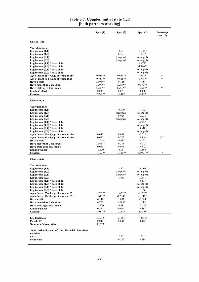
Table 3.7. Couples, initial state (1,1) [both partners working]

Spec. (1) Spec. (2) Spec. (3) Bootstrap

spec. (2) Choice (1,0) Year dummies Log income (1,1) -0.681 -3.498* Log income (1,0) 0.460 3.646* Log income (0,1) (dropped) (dropped) Log income (0,0) (dropped) (dropped) Log income (1,1) * have child 4.477* Log income (1,0) * have child -4.996** Log income (0,1) * have child (dropped) Log income (0,0) * have child (dropped) Age of man: 25-49, age of woman: 25+ -0.684** -0.651** -0.692** ** Age of man: 50-55, age of woman: 25+ -0.651** -0.625** -0.745** ** Have a child 0.193** 0.125 1.154 Have more than 2 children 0.299** 0.287** 0.373** Have child aged less than 5 1.288** 1.256** 1.290** ** London/S.East 0.037 0.078 0.088 Constant -2.992** -1.449 -2.132 Choice (0,1) Year dummies Log income (1,1) -0.809 3.303 Log income (1,0) (dropped) (dropped) Log income (0,1) 0.924 -2.236 Log income (0,0) (dropped) (dropped) Log income (1,1) * have child -4.427 Log income (1,0) * have child (dropped) Log income (0,1) * have child 3.618 Log income (0,0) * have child (dropped) Age of man: 25-49, age of woman: 25+ 0.045 0.099 -0.026 Age of man: 50-55, age of woman: 25+ 0.695 0.722 0.649 (**) Have a child -0.063 -0.087 8.157 Have more than 2 children 0.362** 0.213 0.142 Have child aged less than 5 0.039 0.031 0.042 London/S.East -0.120 -0.111 -0.165 Constant -4.393** -4.321** -12.907** * Choice (0,0) Year dummies Log income (1,1) -1.403 -1.608 Log income (1,0) (dropped) (dropped) Log income (0,1) (dropped) (dropped) Log income (0,0) -1.518 -2.389 Log income (1,1) * have child 0.297 Log income (1,0) * have child (dropped) Log income (0,1) * have child (dropped) Log income (0,0) * have child 1.156 Age of man: 25-49, age of woman: 25+ -1.755** -1.623** -1.652** Age of man: 50-55, age of woman: 25+ -1.675** -1.534* -1.541* Have a child 0.349 1.057 -6.084 Have more than 2 children 0.700 1.195* 1.113 Have child aged less than 5 -0.270 -0.481 -0.456 London/S.East 0.277 0.604 0.617 Constant -4.937** 10.344 15.538 Log likelihood: -7391.5 -7388.9 -7385.2 Pseudo R2 0.041 0.041 0.042 Number of observations: 30,573 Joint insignificance of the financial incentives variables:

Chi2 5.17 12.41 Prob>chi2 0.522 0.414

30

The effect of the financial incentive variables in the couples’ models is summarised in Table 3.8. If the effect of financial incentives goes the way that we might expect a priori, then the coefficient on income in the starting state will be negative, and the coefficient on income in each possible finishing state will be positive; hence we would expect to see (-/+) as the default. This occurs in 9 out of the 12 sets of coefficients in the models. The exceptions are: • for initial state (1,1) and final state (0,0) (where income in state (0,0) has the

‘wrong’ sign; • for initial state (0,1) and final state (1,1) (where income in state (1,1) has the

‘wrong’ sign; • for initial state (0,0) and final state (0,1) where both income variables have the

wrong sign. Thus, the general pattern of results seems sensible. However, in many cases the effects of the financial incentives variables are not significant at the 5% level. This means that when doing the simulations for the employment effects of policy changes in the next section, in many cases the 95% confidence intervals for the employment effects for couples will include zero. In the case of the models for starting states (0,0) and (0,1) this is probably because the LFS does not have a big enough sample size to estimate the effects accurately. In the case of starting state (1,1) the sample size is already very large, and so lack of data seems to be much less of an issue. It may be that including controls for the reason why partners in couples who start the LFS in work leave work by wave 5 (e.g. redundancy) might help identify the effects of financial incentives more clearly. Alternatively, if the reason lies in lack of heterogeneity in terms of financial incentives variables, increasing the number of groups in the process of matching the FRS and LFS samples might produce higher significance of the estimated coefficients. This section presented results based on our preferred definition of the financial incentives variables and our preferred specifications of the transitions models. In Appendix 2 we show results of models based on different definitions of financial incentives variables for comparison. We include four different definitions of financial incentives: a) based on modelled hours and wages but assuming 100% take up of in-work

support; b) based on modelled hours and wages but assuming 100% take up of in-work

support and excluding childcare costs; c) based on actual hours and wages for the sample in work; d) based on modelled wages and the assumption of 40 hours of work for the

calculation of in-work incomes. The Appendix includes results of specification 3 for singles and couples. For couples we also include results of specification 2 for financial incentives variables definitions (a) and (b). Appendix 3 provides some sensitivity analysis of the model. We present simulation results of a 2p tax cut in the basic rate of income tax for models based on different definitions of the financial incentives variables. The tables compare the effect of the reform for our preferred definition with the four other definitions (a-d). It seems that the model is relatively robust with respect to different approaches to modelling financial incentives.

31

Table 3.8. Financial incentives in the couples’ models – summary table, specification 2

Initial state Choice made in time t (1,1) (1,0) (0,1) (0,0) (1,1) n.a. -/+ -/+ (-/-) (1,0) -/+ n.a. -/+ -/+ (0,1) (-/-) -/+ n.a. -/+ (0,0) -/+ -/+ (+/-) n.a. Notes: -/+: both signs as expected (negative sign on income in state at time t-1, and positive on income in time t); combinations of signs in brackets represent cases where one or both signs are not as expected a priori.

32

4. Simulating tax and benefit reforms This section presents the models ‘at work’, with the results from several reform simulations which we run on the estimations. We simulate one reform in detail: a tax cut of 2p in basic income tax rate. 4.1. The simulations A cut in income tax is general enough to allow an overall assessment of the model in terms of conforming to a priori expectations. Among single people, a higher reward in work as a result of the tax cut should, all else remaining constant, encourage higher entry into employment (and lower exit from employment). The result could be ambiguous among people living in couples as higher income in work of one partner might lead to exit (or lower rate of entry) of the other partner. Results of simulations are presented in Tables 4.1 - 4.2. All results presented in this section are based on a grossing up procedure described below. 4.2 Grossing up the results Section 7.4 of Report 2 outlined the problem of appropriate grossing factors which should be used to derive population-level results of the simulations. The grossing method used here is a combination of the two methods suggested in Report 2. The FRS grossing factors are averaged by group (defined in the same way as for the purpose of transferring the financial incentives variables) in the FRS and transferred across to the LFS. They are then appropriately weighted to make sure that the sum of grossing factors for a given group in the LFS is the same as in the FRS. Table 4.1 gives an example of how we derive the grossing factors for individuals and couples in the LFS. This procedure avoids the problems described in Report 2 and ensures that according to the characteristics by which we group the data, the population sums are the same in the LFS model and in the FRS data sets.

Table 4.1. Using FRS grossing factors in the LFS – an example.

Grossing factors:

Individual for group A in

FRS

Sum for group A in FRS

Average for group A

Individual for group A in

LFS

Sum for group A in LFS

Weighed individual for

group A in LFS

1) 1,050 a) 1,456 a) 1,040 2) 980 b) 1,456 b) 1,040 3) 1,360 7,280 1,456 c) 1,456 10,192 c) 1,040 4) 1,520 d) 1,456 d) 1,040 5) 2,370 e) 1,456 e) 1,040

f) 1,456 f) 1,040 g) 1,456 g) 1,040

33

4.3 Short and long-run (equilibrium) effects. In Report 2 (2:7.5) we demonstrated how both short and long run employment effects of tax and benefit simulations can be derived using the model. Short run effects are ‘immediate-response’ effects following a tax and benefit reform. Long run results are calculated assuming that the change in financial incentives creates a permanent change in the entry and exit rates for individuals and thus leads to a new level of employment in the labour market equilibrium. In the underlying assumption of market equilibrium the long run effects are similar to the simulated effects using structural models. Of course both from the researcher’s and the policy-maker’s point of view it is interesting how ‘far’ the short run effects are from the long-run effects or in other words how quickly, given the exit and entry rates, the market converges to the new equilibrium. In the simulation results section below we present convergence charts, which demonstrate the speed of labour market adjustment to equilibrium. The results tables give both short and long run effects of the simulations. Long-run effects are based on the definition of equilibrium as a state for which in a given sub-sample the number of people entering and exiting employment is the same. Since we model singles and couples separately, equilibria are defined separately for singles and couples. Because an equilibrium defined as, for example, “the number of men without children entering and exiting employment” is to say the least peculiar, we do not disaggregate the long-run effects any further. For people in couples we can identify the long run effects separately for men and women, as we know the equilibrium number of couples in different employment states. 4.4 Simulation results. As we expected, a 2p tax cut in the basic rate of income tax leads to a positive (and statistically significant8) employment effect among single individuals, which is high especially among those without children. For several reasons, those with children are less responsive to this simulated reform. First of all, as we noted above, responsiveness to financial incentives among people with children who are out of work is lower than among people without children. Secondly, especially for those on low wages who are eligible for in-work support, the effect of the tax cut for people with children is reduced because of the partial withdrawal of benefits. The tax cut has a very modest effect on individuals in couples. This positive effect is not statistically significant. Couples with children are more responsive than those without children, but the positive effect on employment of men is almost exactly matched by a negative effect on employment of women. If we look at Table 4.3 we can see that this is a result of the increase in the number of one-earner couples with the man in work and woman out of work. The number of couples where no one works and where both partners are employed is reduced as a result of the tax cut. Table 4.3 shows a transition matrix for the short run effect of the 2p tax cut. The vertical columns refer to the state in time (t-1) while horizontal to the state in time t. The cells show the difference in the number of couples in a given ‘row’ state in time (t) conditional on being in a given ‘column’ state in time (t-1). 8 Statistical significance was tested on the basis of a bootstrap exercise with 1000 separate draws from FRS and LFS samples.

34

Table 4.2. Short run effect on employment of a 2p tax cut Short-run Long-run All People without

children People with

children All

Couples: Men 1,200 200 1,000 2100 Women -900 -100 -700 -2200 Total 300 100 300 -100 Singles: Men 10,000 9,900 0 - Women 2,500 1,900 600 - Total 12,500 11,800 600 22,400 Overall: 12,800 11,900 900 22,300 Numbers might not add up due to rounding (to nearest 100) Based on FRS grossing factors. Simulation based on specification 3 for singles and specification 2 for couples. Singles simulations: Long run effect can only be calculated for the overall sample, i.e. based on the definition of equilibrium as a state in which the same number of singles (regardless of gender) enters and exits employment.

Table 4.3. Change in the number of couples in different employment states as a result of a 2p tax cut.

Couples in (t-1)

(1,1) couples (1,0) couples (0,1) couples (0,0) couples Initial grossed-up number of couples: 4,600,000 1,300,000 300,000 250,000 Short run effect: - Couples with children -500 1500 -200 -800 - Couples without children -200 500 100 -400 Long run: -1,800 3,900 -500 -1600 Transitions in the short run: Couples in (t): (1,1) couples 400 -500 -1300 600 (1,0) couples -100 200 2200 -400 (0,1) couples -100 200 -100 -200 (0,0) couples -200 0 -800 -100

Numbers might not add up due to rounding (to nearest 100) Based on FRS grossing factors (see footnote 7). Simulation based on specification 2. In tables 4.2 and 4.3 we show both short-run and long run effects of the simulation. Figure 4.1 shows the speed of adjustment from short to long-run equilibrium for

35

singles and couples. We can see that most of the adjustment to equilibrium takes place in the first few iterations.

Figure 4.1 Convergence to long-run effects of 2p tax cut simulation.

iteration

men women all

0 5 10 15 20 25 30 35 40

0

2500

10000

20000

25000

iteration

men_diff women_diff all_diff

0 5 10 15 20 25 30 35 40

-2500

0

2400

Singles Couples

Notes: Singles simulations: overall long run effect does not equal to the sum of effects estimated separately for men and women as these define equilibrium as a state in which the same number of men (or women) enter and exit employment.

36

5 Conclusions In this project we have developed and estimated a dynamic model of labour market transitions on UK data between 1996 and 2001. The basic structure of the model is based on earlier research by Gregg et al. (1999) but we regard this project as an advance in several ways over previous models in the literature. The model we propose includes modelling of fixed cost of working and take-up of in-work benefits. The structure of the model presented for individuals in couples is an original application of multinomial choice modelling in the context of dynamic labour supply. This is a significant advancement over the methodology which models one partner’s labour supply decisions conditional on the other partner’s behaviour. On top of this the model has been applied to data sets constructed from five years of FRS and LFS data. Given differentiation in financial incentives over time this provides for better identification of the effect of financial incentives on individual labour market behaviour. We have identified some interesting effects of financial incentives on labour market behaviour of single people with children. First of all while working single parents demonstrate higher responsiveness to financial incentives than childless people, single people with children who are out of work seem to be less responsive to financial incentives. We believe that this finding deserves more detailed analysis. Secondly, related to this is the finding that as far as work entry is concerned, differentiation of responsiveness to financial incentives is at the level of gender and not family structure. Single women (with and without children) seem to be less responsive to financial incentives than single men. Once again it is interesting that such differentiation does not apply to the exit model, which, one could think, is just the ‘reverse’ side of the entry decisions in the labour market. Our concerns regarding the model for couples largely focus around the fact that in two out of four cases it does not produce a (jointly) statistically significant influence of financial incentives on labour market behaviour for some subgroups we model. Part of the blame for this result can be ascribed to small sample size in the case of the (0,0) sample of couples. But this explanation cannot be supported for the sample of two-earner couples (1,1), where we also could not reject the hypothesis of no (joint) effect of financial incentives on labour market transitions. In the latter case one possible reason for this lack of significance is that some of the exits are not the direct result of individual choice – for example, redundancies, or a decision to move out of a job because one’s partner wants to move to a different region. It would be useful to experiment with adding extra LFS information on the reason for leaving the job into the model. Another possible explanation is insufficient heterogeneity in (group level) financial incentives given the size of the sample. It would certainly be interesting to analyse these two hypotheses further. Apart from the further analysis suggested above, the project has opened up new avenues for further research. First of all we believe that applying the methodology developed in this project to individual level panel data sets (i.e. without the necessity to match group level financial incentives between two surveys) would result in a model with greater precision of estimated effects of financial incentives. This type of analysis could be done using the BHPS and/or FACS, provided that tax and benefit models are developed and applied to these data sets with the same rigour as for the

37

FRS. Another advantage of using a multiple wave panel data set would be an opportunity to apply more advanced methods of estimation (for example Generalised Method of Moments). During the development of the project we have also examined and analysed options for using the model to make inferences about what will happen to the distribution of income as a result of changes in employment following tax and benefit reforms. Appendix 5 presents our initial thoughts concerning the methodology which could be used for such an extension.

38

Appendix 1. Intermediate models. Stages 1 and 3 of the modelling process

Table A1.1 Wage equations. OLS wage equation Heckman wage equation Entry wage -

men Entry wage -

women Overall wage -

men Overall wage -

women Dependent variable: Log LFS entry

wage Log LFS entry

wage Log FRS wage Log FRS wage

Year dummies Included Included Included Included (Age-16) 0.008 0.057** 0.081** 0.108** (Age-16)2 0.001 -0.003** -0.002** -0.004** (Age-16)3 0.000 0.000** 0.000** 0.000** Left school aged 17-18 0.112** 0.145** 0.254** 0.236** Left school aged 19+ 0.308** 0.391** 0.476** 0.521** London/S.East 0.046 0.168** 0.166** 0.151** Married 0.079** 0.026 0.211** 0.027* Has a child - - - -0.186** Constant 1.193** 0.868** 0.853** 0.703** Selection variables: Λ - - 0.263** 0.090** Ρ - - 0.507** 0.184** Log likelihood: - - -44820.0 -50236.1 R2 0.130 0.161 - - Number of observations 1342 2533 46047 49227 - censored - - 5473 12584 - uncensored - - 40574 36643 Source: based on LFS for OLS wage equations and FRS for Heckman wage equations (1997/98-2001/02).

39

Table A1.2 Hours regressions. Single men,

no children Single women,

no children Single parents Married men Married

women Dependent variable: usual hours worked (for those employed)

Year dummies Included Included Included Included Included Region 1 0.137 -0.818 -1.284 -0.460 -0.570 Region 2 -0.401 -0.270 -0.946 0.303 -0.700** Region 3 -0.294 -0.611 -0.035 -0.486* 0.326 Region 4 0.517 0.478 -0.812 0.318 -0.634** Region 5 -1.001** 0.737 -0.367 0.071 -0.033 Region 6 1.687** 1.097** -2.477** 1.765** -1.462** Region 7 0.033 0.546 1.791** -0.450* 1.023** Region 8 0.371 1.451** 0.004 0.314 -0.928** Region 9 -0.428 0.196 -0.890 0.108 -1.548** Region 10 -0.624 0.156 -2.630** -0.050 -0.580 Left school aged 17-18 -1.989** 1.150** 2.414** -2.269** 1.767** Left school aged 19+ -3.102** 0.651** 5.163** -2.929** 3.281** Have a child - - - 0.335** -4.842** Have more than 2 children - - -2.432** -0.474** -2.252** Youngest child aged 0-1 - - -4.547** 0.199 -3.658** Youngest child aged 2-4 - - -5.665** 0.355* -4.625** Youngest child aged 5-10 - - -4.473** 0.314* -3.550** Constant 42.801** 36.091** 28.937** 43.977** 33.350** R2 0.02 0.01 0.07 0.02 0.15 Number of observations 10692 8311 4027 29736 25118 Source: based on FRS 1997/98-2001/02.

40

Table A1.3 Hourly cost of childcare. Dependent variable: Hourly

childcare cost Year dummies Included Region 1 -0.201 Region 2 0.039 Region 3 -0.110 Region 4 0.050 Region 5 -0.095 Region 6 0.323** Region 7 0.551** Region 8 0.383** Region 9 0.220** Region 10 -0.168 Youngest child aged 0-1 -0.349** Youngest child aged 2-4 -0.436** Youngest child aged 5-10 -0.232* Constant 2.193** R2 0.05 Number of observations 3994

Source: based on FRS 1997/98-2001/02.

41

Table A1.4 Singles – childcare hours and take-up equations and FC/WFTC take up.

Hours of paid

childcare among those who use it

Use of paid childcare

Take-up of FC/WFTC

Dependent variable: Log childcare

hours Paid childcare

dummy FC/WFTC

claim dummy Year dummies Included Included Included Age: 25-36 0.173* 0.359** - Age: 37-49 0.054 0.229* - Age: 50-55 -0.103 0.207 - Male 0.220** -0.221** -0.302** Education: left school aged 17-18 0.010 0.135** -0.258** Education: left school aged 19+ -0.036 0.452** -0.569** London/S.East 0.158 0.051 -0.403** Youngest child aged 0-1 0.954** 1.713** 0.229 Youngest child aged 2-4 0.709** 1.972** 0.327** Youngest child aged 5-10 0.154 1.308** 0.294** Has more than 2 children 0.485** -0.195** 0.169 Hourly childcare cost -0.254 - - Non-employed member of HH - -0.831** - FC/WFTC eligibility - - 0.005** Works less than 30 hours per week -0.561** -0.787** 0.561** Constant 3.078** -1.820** -0.031 Log likelihood: - -1479.3 -893.6 (Pseudo) R2 0.31 0.23 0.17 Number of observations 849 3461 1710

Source: based on FRS 1997-2001.

42

Table A1.5 Couples – childcare hours and take-up equations and FC/WFTC take up.

Hours of paid

childcare among those

who use it

Use of paid childcare, 01,

10 couples

Use of paid childcare, 11

couples

Take-up of FC/WFTC

Dependent variable: Log childcare

hours Paid childcare

dummy Paid childcare

dummy FC/WFTC

claim dummy Year dummies Included Included Included Included Left school: man: <16, woman 17-18 -0.002 0.337** 0.234** -0.202** Left school: man: <16, woman 19+ 0.042 0.561** 0.542** -0.726** Left school: man: 17-18, woman <16 0.159** 0.091 0.139** -0.144 Left school: man: 17-18, woman 17-18 0.062 0.331** 0.364** -0.656** Left school: man: 17-18, woman 19+ 0.039 0.598** 0.641** -0.727** Left school: man: 19+, woman <16 0.068 0.351** 0.242** -0.492** Left school: man: 19+, woman 17-18 0.026 0.566** 0.545** -0.215 Left school: man: 19+, woman 19+ 0.101** 0.729** 0.876** -0.612** London/S.East 0.149** -0.136** 0.007 -0.144* Youngest child aged 0-1 1.156** 1.264** 2.022** 0.436** Youngest child aged 2-4 0.991** 1.232** 2.075** 0.375** Youngest child aged 5-10 0.287** 0.822** 1.395** 0.297** Have more than 2 children 0.070** -0.244** -0.320** 0.268** Hourly childcare cost -0.144 - - - Non-employed member of HH - -0.187 -0.494** - FC/WFTC eligibility - - - 0.005** Employment: man part-time, woman not working -1.097** - - 1.653** Employment: man not working, woman part-time -0.464** 0.550** - 1.189** Employment: man not working, woman full-time -0.089 1.202** - 1.079** Employment: man full-time, woman not working -0.785** 0.327 - 1.013** Employment: man part-time, woman part-time -0.428** - -0.861** 1.105** Employment: man part-time, woman full-time -0.532** - -0.323** 0.873* Employment: man full-time, woman part-time -0.567** - -0.682** 0.379* Constant 2.690** -3.586** -1.969** -1.406** Log likelihood: - -928.0 -5076.2 -1043.4 (Pseudo) R2 0.32 0.12 0.24 0.21 Number of observations 3243 5685 11878 1927 Source: based on FRS 1997/98-2001/02.

43

Appendix 2 – Different definitions of financial incentives variables. A2.1 Singles Results of specification 3 applied to three different definitions of income: including FC take-up modelling and childcare costs excluding FC take-up modelling but including childcare costs excluding both FC take-up modelling and childcare modelling

Table A2.1 Robustness check: singles – entry model, specification 3, modelling take-up and childcare.

Spec. (3)

Modelled FC and CC

Spec. (3) 100% FC take-up, included CC

Spec. (3) 100% FC take-up, excluded CC

Entry Year dummies Included Included Included Log income out of work -1.381** -1.420** -1.410** Log income in work 1.991** 2.119** 2.120** Log income out of work * single parent 0.645 0.263 0.184 Log income in work * single parent -0.966** -0.601 -0.543 Log income out of work * childless female 0.605** 0.664** 0.661** Log income in work * childless female -0.989** -1.065** -1.063** Age: 25-36 -0.326** -0.329** -0.336** Age: 37-49 -0.627** -0.650** -0.657** Age: 50-55 -1.039** -1.068** -1.076** Has a child 1.970 1.899 1.972 Has more than 2 children -0.224** -0.184* -0.181* Has child aged less than 5 -0.462** -0.460** -0.488** Female with child 0.276** 0.290** 0.289** Female without child 2.873** 3.027** 3.031** London/S.East -0.081* -0.097** -0.102** Constant -4.394** -4.872** -4.915** Log likelihood: -4155.4 -4150.8 -4149.5 Pseudo R2 0.1097 0.1107 0.1109 Number of observations 8662

44

Table A2.2 Robustness check: singles – exit model, specification 3, modelling take-up and childcare.

Spec. (3)

Modelled FC and CC

Spec. (3) 100% FC take-up, included CC

Spec. (3) 100% FC take-up, excluded CC

Exit Year dummies Included Included Included Log income out of work 0.127 0.155 0.145 Log income in work -0.500** -0.528** -0.531** Log income out of work * single parent 0.956** 0.896** 0.882** Log income in work * single parent -0.868** -0.817** -0.809** Log income out of work * childless female -0.067 -0.089 -0.087 Log income in work * childless female 0.096 0.111 0.110 Age: 25-36 -0.101** -0.102** -0.097** Age: 37-49 -0.089* -0.087* -0.083 Age: 50-55 0.063 0.063 0.068 Has a child -0.066 -0.010 0.037 Has more than 2 children 0.128 0.118 0.123 Has child aged less than 5 0.390** 0.395** 0.428** Female with child 0.208** 0.205** 0.207** Female without child -0.519 -0.513 -0.513 London/S.East 0.186** 0.191** 0.196** Constant 0.447 0.474 0.524 Log likelihood: -5153.7 -5152.9 -5151.4 Pseudo R2 0.0458 0.0459 0.0462 Number of observations 31651

45

Results of specification 3 applied to three different definitions of income: With modelled hours and wages for all With 40 hours and modelled wages for all With data hours and wages for those for whom we have these

Table A2.3 Robustness check: singles – entry model, specification 3, modelling hours and wages.

Spec. (3)

Modelled hours and

wages for all

Spec. (3) 40 hours when

in work

Spec. (3) Data hours and

wages when in work

Entry Year dummies Included Included Included Log income out of work -1.381** -1.355** - Log income in work 1.991** 1.848** - Log income out of work * single parent 0.645 0.869** - Log income in work * single parent -0.966** -1.130** - Log income out of work * childless female 0.605** 0.547** - Log income in work * childless female -0.989** -0.835** - Age: 25-36 -0.326** -0.307** - Age: 37-49 -0.627** -0.597** - Age: 50-55 -1.039** -0.998** - Has a child 1.970 1.595 - Has more than 2 children -0.224** -0.207** - Has child aged less than 5 -0.462** -0.420** - Female with child 0.276** 0.283** - Female without child 2.873** 2.198** - London/S.East -0.081* -0.064 - Constant -4.394** -3.718** - Log likelihood: -4155.4 41.51.7 - Pseudo R2 0.1097 0.1105 - Number of observations 8662

46

Table A2.4 Robustness check: singles – exit model, specification 3, modelling hours and wages.

Spec. (3)

Modelled hours and

wages for all

Spec. (3) 40 hours when

in work

Spec. (3) Data hours and

wages when in work

Exit Year dummies Included Included Included Log income out of work 0.127 0.118 -0.011 Log income in work -0.500** -0.468** -0.451** Log income out of work * single parent 0.956** 0.805** 0.731** Log income in work * single parent -0.868** -0.780** -0.508** Log income out of work * childless female -0.067 -0.037 -0.010 Log income in work * childless female 0.096 0.052 0.038 Age: 25-36 -0.101** -0.105** -0.054 Age: 37-49 -0.089* -0.092* -0.045 Age: 50-55 0.063 0.056 0.102 Has a child -0.066 0.370 -0.674 Has more than 2 children 0.128 0.118 0.093 Has child aged less than 5 0.390** 0.316** 0.394** Female with child 0.208** 0.170 0.082 Female without child -0.519 -0.364 -0.474 London/S.East 0.186** 0.179** 0.197** Constant 0.447 0.302 0.801 Log likelihood: -5153.7 -5150.5 -5152.9 Pseudo R2 0.0458 0.464 0.0459 Number of observations 31651

47

A2.2 Couples Results of specification 3 applied to three different definitions of income: Including FC take-up modelling and childcare costs Excluding FC take-up modelling but including childcare costs Excluding both FC take-up modelling and childcare modelling

48

Table A2.5 Robustness check: couples (0,0), specification 3, modelling take-up and childcare.

Spec. (3)

Modelled FC and CC

Spec. (3) 100% FC take-up, included CC

Spec. (3) 100% FC take-up, excluded CC

Choice (1,1) Year dummies Included Included Included Log income (1,1) 3.880 3.888 3.923 Log income (1,0) (dropped) (dropped) (dropped) Log income (0,1) (dropped) (dropped) (dropped) Log income (0,0) -2.848** -2.846** -2.853** Log income (1,1) * have child -3.429 -3.444 -3.389 Log income (1,0) * have child (dropped) (dropped) (dropped) Log income (0,1) * have child (dropped) (dropped) (dropped) Log income (0,0) * have child 3.365** 3.365** 3.329** Age of man: 25-49, age of woman: 25+ -1.257** -1.258** -1.266** Age of man: 50-55, age of woman: 25+ -2.459** -2.463** -2.476** Have a child 3.123 3.212 3.073 Have more than 2 children -1.141** -1.149** -1.136** Have child aged less than 5 -0.953** -0.958** -0.970** London/S.East -0.360 -0.360 -0.370 Constant -8.623 -8.679 -8.834 Choice (1,0) Year dummies Included Included Included Log income (1,1) (dropped) (dropped) (dropped) Log income (1,0) 2.967 2.963 2.976 Log income (0,1) (dropped) (dropped) (dropped) Log income (0,0) -1.225 -1.223 -1.230 Log income (1,1) * have child (dropped) (dropped) (dropped) Log income (1,0) * have child -3.351 -3.368 -3.330 Log income (0,1) * have child (dropped) (dropped) (dropped) Log income (0,0) * have child 0.962 0.969 0.952 Age of man: 25-49, age of woman: 25+ -0.238 -0.239 -0.242 Age of man: 50-55, age of woman: 25+ -0.448 -0.450 -0.456 Have a child 14.706** 14.771** 14.646** Have more than 2 children 0.205 0.215 0.210 Have child aged less than 5 0.071 0.071 0.075 London/S.East 0.180 0.181 0.179 Constant -11.671* -11.655* -11.693* Choice (0,1) Year dummies Included Included Included Log income (1,1) (dropped) (dropped) (dropped) Log income (1,0) (dropped) (dropped) (dropped) Log income (0,1) 1.628 1.625 1.632 Log income (0,0) -0.946 -0.965 -0.971 Log income (1,1) * have child (dropped) (dropped) (dropped) Log income (1,0) * have child (dropped) (dropped) (dropped) Log income (0,1) * have child -3.596 -3.743 -3.688 Log income (0,0) * have child 2.041 2.097 2.046 Age of man: 25-49, age of woman: 25+ -1.014* -1.015* -1.019** Age of man: 50-55, age of woman: 25+ -1.979** -1.976** -1.983** Have a child 9.301 9.913 9.882 Have more than 2 children -0.090 -0.064 -0.071 Have child aged less than 5 -0.557 -0.567* -0.545 London/S.East -1.775** -1.770** -1.762** Constant -5.149 -5.032 -5.040 Log likelihood: -819.0 -818.9 -818.9 Pseudo R2 0.056 0.056 0.056 Number of observations: 872 Joint insignificance of the financial incentives variables: Chi2 11.63 11.66 11.68 Prob>chi2 0.476 0.473 0.472

49

Table A2.6 Robustness check: couples (0,1), specification 3, modelling take-up and childcare.

Spec. (3)

Modelled FC and CC

Spec. (3) 100% FC take-up, included CC

Spec. (3) 100% FC take-up, excluded CC

Choice (1,1) Year dummies Included Included Included Log income (1,1) 4.919* 4.837* 4.861* Log income (1,0) (dropped) (dropped) (dropped) Log income (0,1) -3.799* -3.726* -3.744* Log income (0,0) (dropped) (dropped) (dropped) Log income (1,1) * have child -5.847** -6.219** -6.128** Log income (1,0) * have child (dropped) (dropped) (dropped) Log income (0,1) * have child 3.821* 4.233** 4.136* Log income (0,0) * have child (dropped) (dropped) (dropped) Age of man: 25-49, age of woman: 25+ -0.108 -0.094 -0.099 Age of man: 50-55, age of woman: 25+ -0.500 -0.508 -0.510 Have a child 14.149* 14.107* 14.102* Have more than 2 children -0.494 -0.576* -0.562* Have child aged less than 5 -0.055 -0.051 -0.015 London/S.East -0.322 -0.316 -0.314 Constant -8.352 -8.263 -8.303 Choice (1,0) Year dummies Included Included Included Log income (1,1) (dropped) (dropped) (dropped) Log income (1,0) 7.544* 7.426* 7.446* Log income (0,1) -5.407 -5.177 -5.197 Log income (0,0) (dropped) (dropped) (dropped) Log income (1,1) * have child (dropped) (dropped) (dropped) Log income (1,0) * have child -8.436 -9.736 -9.165 Log income (0,1) * have child 8.050 9.606 9.055 Log income (0,0) * have child (dropped) (dropped) (dropped) Age of man: 25-49, age of woman: 25+ -1.512 -1.471 -1.458 Age of man: 50-55, age of woman: 25+ -2.828* -2.913** -2.884** Have a child 2.329 0.969 0.759 Have more than 2 children -0.431 -0.559 -0.506 Have child aged less than 5 0.824 0.878 0.818 London/S.East -0.859 -0.870 -0.903 Constant -12.949 -13.548 -13.550 Choice (0,0) Year dummies Included Included Included Log income (1,1) (dropped) (dropped) (dropped) Log income (1,0) (dropped) (dropped) (dropped) Log income (0,1) -0.982 -0.980 -0.998 Log income (0,0) 0.858 0.775 0.738 Log income (1,1) * have child (dropped) (dropped) (dropped) Log income (1,0) * have child (dropped) (dropped) (dropped) Log income (0,1) * have child -0.463 -1.027 -1.267 Log income (0,0) * have child 2.532 3.074 3.279 Age of man: 25-49, age of woman: 25+ (dropped) (dropped) (dropped) Age of man: 50-55, age of woman: 25+ -1.694** -1.667** -1.635** Have a child -11.092 -10.702 -10.426 Have more than 2 children -0.985 -1.018* -1.036* Have child aged less than 5 0.834* 0.845* 0.871* London/S.East 0.233 0.208 0.208 Constant -1.057 -0.685 -0.435 Log likelihood: -680.7 -679.9 -679.8 Pseudo R2 0.044 0.045 0.046 Number of observations: 769 Joint insignificance of the financial incentives variables: Chi2 20.63 22.26 22.12 Prob>chi2 0.056 0.035 0.036

50

Table A2.7 Robustness check: couples (1,0), specification 3, modelling take-up and childcare.

Spec. (3)

Modelled FC and CC

Spec. (3) 100% FC take-up, included CC

Spec. (3) 100% FC take-up, excluded CC

Choice (1,1) Year dummies Included Included Included Log income (1,1) 5.788** 5.658** 5.630** Log income (1,0) -5.151** -5.047** -5.026** Log income (0,1) (dropped) (dropped) (dropped) Log income (0,0) (dropped) (dropped) (dropped) Log income (1,1) * have child -5.262** -5.619** -5.746** Log income (1,0) * have child 4.136* 4.480* 4.607** Log income (0,1) * have child (dropped) (dropped) (dropped) Log income (0,0) * have child (dropped) (dropped) (dropped) Age of man: 25-49, age of woman: 25+ -0.109 -0.114 -0.114 Age of man: 50-55, age of woman: 25+ -0.756** -0.757** -0.756** Have a child 8.449** 8.620** 8.663** Have more than 2 children -0.223** -0.234** -0.243** Have child aged less than 5 -0.490** -0.502** -0.500** London/S.East -0.159* -0.156* -0.155* Constant -6.454** -6.266** -6.223** Choice (0,1) Year dummies Included Included Included Log income (1,1) (dropped) (dropped) (dropped) Log income (1,0) 2.860 2.773 2.734 Log income (0,1) -4.677 -4.619 -4.568 Log income (0,0) (dropped) (dropped) (dropped) Log income (1,1) * have child (dropped) (dropped) (dropped) Log income (1,0) * have child -5.928 -5.714 -5.820 Log income (0,1) * have child 9.118* 9.123* 9.222* Log income (0,0) * have child (dropped) (dropped) (dropped) Age of man: 25-49, age of woman: 25+ (dropped) (dropped) (dropped) Age of man: 50-55, age of woman: 25+ 0.768 0.815* 0.817* Have a child -12.639 -14.236 -14.159 Have more than 2 children -0.522 -0.506 -0.505 Have child aged less than 5 -0.431 -0.418 -0.477 London/S.East -0.182 -0.156 -0.158 Constant 2.314 2.448 2.413 Choice (0,0) Year dummies Included Included Included Log income (1,1) (dropped) (dropped) (dropped) Log income (1,0) -0.341 -0.331 -0.332 Log income (0,1) (dropped) (dropped) (dropped) Log income (0,0) -0.182 -0.203 -0.205 Log income (1,1) * have child (dropped) (dropped) (dropped) Log income (1,0) * have child -2.313* -2.352* -2.353* Log income (0,1) * have child (dropped) (dropped) (dropped) Log income (0,0) * have child 0.711 0.788 0.787 Age of man: 25-49, age of woman: 25+ -0.830** -0.848** -0.850** Age of man: 50-55, age of woman: 25+ -0.331 -0.348 -0.351 Have a child 10.130 9.990 10.000 Have more than 2 children 0.798** 0.810** 0.807** Have child aged less than 5 -0.371** -0.366* -0.355* London/S.East 0.815** 0.804** 0.804** Constant -0.280 -0.231 -0.218 Log likelihood: -4667.0 -4668.4 -4668.2 Pseudo R2 0.022 0.022 0.022 Number of observations: 7245 Joint insignificance of the financial incentives variables: Chi2 40.84 39.61 39.93 Prob>chi2 0.000 0.000 0.0001

51

Table A2.8 Robustness check: couples (1,1), specification 3, modelling take-up and childcare.

Spec. (3) Modelled FC

and CC

Spec. (3) 100% FC take-up, included CC

Spec. (3) 100% FC take-up, excluded CC

Choice (1,0) Year dummies Included Included Included Log income (1,1) -3.498* -3.610* -3.615* Log income (1,0) 3.646* 3.777* 3.782* Log income (0,1) (dropped) (dropped) (dropped) Log income (0,0) (dropped) (dropped) (dropped) Log income (1,1) * have child 4.477* 3.515 3.767* Log income (1,0) * have child -4.996** -3.975* -4.234* Log income (0,1) * have child (dropped) (dropped) (dropped) Log income (0,0) * have child (dropped) (dropped) (dropped) Age of man: 25-49, age of woman: 25+ -0.692** -0.699** -0.701** Age of man: 50-55, age of woman: 25+ -0.745** -0.755** -0.758** Have a child 1.154 1.129 1.087 Have more than 2 children 0.373** 0.320** 0.335** Have child aged less than 5 1.290** 1.260** 1.266** London/S.East 0.088 0.066 0.067 Constant -2.132 -2.193 -2.181 Choice (0,1) Year dummies Included Included Included Log income (1,1) 3.303 3.514 3.516 Log income (1,0) (dropped) (dropped) (dropped) Log income (0,1) -2.236 -2.391 -2.393 Log income (0,0) (dropped) (dropped) (dropped) Log income (1,1) * have child -4.427 -4.199 -4.195 Log income (1,0) * have child (dropped) (dropped) (dropped) Log income (0,1) * have child 3.618 3.208 3.191 Log income (0,0) * have child (dropped) (dropped) (dropped) Age of man: 25-49, age of woman: 25+ -0.026 -0.044 -0.046 Age of man: 50-55, age of woman: 25+ 0.649 0.646 0.645 Have a child 8.157 8.861 8.933 Have more than 2 children 0.142 0.233 0.237 Have child aged less than 5 0.042 0.051 0.055 London/S.East -0.165 -0.168 -0.167 Constant -12.907** -13.382** -13.385** Choice (0,0) Year dummies Included Included Included Log income (1,1) -1.608 -1.602 -1.616 Log income (1,0) (dropped) (dropped) (dropped) Log income (0,1) (dropped) (dropped) (dropped) Log income (0,0) -2.389 -2.389 -2.392 Log income (1,1) * have child 0.297 0.317 0.282 Log income (1,0) * have child (dropped) (dropped) (dropped) Log income (0,1) * have child (dropped) (dropped) (dropped) Log income (0,0) * have child 1.156 1.171 1.136 Age of man: 25-49, age of woman: 25+ -1.652** -1.656** -1.651** Age of man: 50-55, age of woman: 25+ -1.541* -1.544* -1.541* Have a child -6.084 -6.282 -5.889 Have more than 2 children 1.113 1.109 1.116 Have child aged less than 5 -0.456 -0.452 -0.419 London/S.East 0.617 0.613 0.624 Constant 15.538 15.509 15.602 Log likelihood: -7385.2 -7386.2 -7386.2 Pseudo R2 0.042 0.042 0.042 Number of observations: 30573 Joint insignificance of the financial incentives variables: Chi2 12.41 10.36 10.38 Prob>chi2 0.414 0.585 0.583

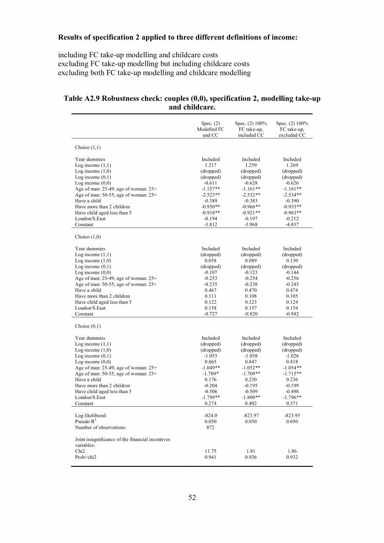
52

Results of specification 2 applied to three different definitions of income: including FC take-up modelling and childcare costs excluding FC take-up modelling but including childcare costs excluding both FC take-up modelling and childcare modelling

Table A2.9 Robustness check: couples (0,0), specification 2, modelling take-up and childcare.

Spec. (2)

Modelled FC and CC

Spec. (2) 100% FC take-up, included CC

Spec. (2) 100% FC take-up, excluded CC

Choice (1,1) Year dummies Included Included Included Log income (1,1) 1.217 1.259 1.269 Log income (1,0) (dropped) (dropped) (dropped) Log income (0,1) (dropped) (dropped) (dropped) Log income (0,0) -0.611 -0.628 -0.626 Age of man: 25-49, age of woman: 25+ -1.157** -1.161** -1.161** Age of man: 50-55, age of woman: 25+ -2.523** -2.532** -2.534** Have a child -0.389 -0.383 -0.390 Have more than 2 children -0.950** -0.966** -0.953** Have child aged less than 5 -0.918** -0.921** -0.963** London/S.East -0.194 -0.197 -0.212 Constant -3.812 -3.968 -4.037 Choice (1,0) Year dummies Included Included Included Log income (1,1) (dropped) (dropped) (dropped) Log income (1,0) 0.058 0.089 0.130 Log income (0,1) (dropped) (dropped) (dropped) Log income (0,0) -0.107 -0.123 -0.144 Age of man: 25-49, age of woman: 25+ -0.253 -0.254 -0.256 Age of man: 50-55, age of woman: 25+ -0.235 -0.238 -0.245 Have a child 0.467 0.470 0.474 Have more than 2 children 0.111 0.108 0.105 Have child aged less than 5 0.122 0.123 0.124 London/S.East 0.158 0.157 0.154 Constant -0.727 -0.820 -0.942 Choice (0,1) Year dummies Included Included Included Log income (1,1) (dropped) (dropped) (dropped) Log income (1,0) (dropped) (dropped) (dropped) Log income (0,1) -1.053 -1.058 -1.026 Log income (0,0) 0.865 0.847 0.818 Age of man: 25-49, age of woman: 25+ -1.049** -1.052** -1.054** Age of man: 50-55, age of woman: 25+ -1.709* -1.709** -1.715** Have a child 0.176 0.230 0.236 Have more than 2 children -0.204 -0.195 -0.199 Have child aged less than 5 -0.506 -0.509 -0.498 London/S.East -1.799** -1.800** -1.796** Constant 0.274 0.402 0.371 Log likelihood: -824.0 -823.97 -823.95 Pseudo R2 0.050 0.050 0.050 Number of observations: 872 Joint insignificance of the financial incentives variables: Chi2 11.75 1.81 1.86 Prob>chi2 0.941 0.936 0.932

53

Table A2.10 Robustness check: couples (0,1), specification 2, modelling take-up and childcare.

Spec. (2)

Modelled FC and CC

Spec. (2) 100% FC take-up, included CC

Spec. (2) 100% FC take-up, excluded CC

Choice (1,1) Year dummies Included Included Included Log income (1,1) -0.187 -0.549 -0.483 Log income (1,0) (dropped) (dropped) (dropped) Log income (0,1) -0.438 -0.123 -0.190 Log income (0,0) (dropped) (dropped) (dropped) Age of man: 25-49, age of woman: 25+ -0.110 -0.102 -0.111 Age of man: 50-55, age of woman: 25+ -0.615 -0.639 -0.641 Have a child -0.432** -0.439** -0.432** Have more than 2 children -0.429 -0.483 -0.474 Have child aged less than 5 -0.037 -0.043 -0.023 London/S.East -0.311 -0.310 -0.307 Constant 4.245 4.704 4.679 Choice (1,0) Year dummies Included Included Included Log income (1,1) (dropped) (dropped) (dropped) Log income (1,0) 3.757 4.426 4.535 Log income (0,1) -1.645 -1.944 -2.060 Log income (0,0) (dropped) (dropped) (dropped) Age of man: 25-49, age of woman: 25+ -1.630 -1.651 -1.665 Age of man: 50-55, age of woman: 25+ -3.024** -3.141** -3.147** Have a child -1.083 -1.141* -1.145* Have more than 2 children -0.196 -0.310 -0.304 Have child aged less than 5 0.808 0.836 0.836 London/S.East -0.993 -0.981 -0.968 Constant -12.278* -14.291** -14.255** Choice (0,0) Year dummies Included Included Included Log income (1,1) (dropped) (dropped) (dropped) Log income (1,0) (dropped) (dropped) (dropped) Log income (0,1) -1.023 -1.255 -1.416 Log income (0,0) 2.609** 2.785** 2.874** Age of man: 25-49, age of woman: 25+ (dropped) (dropped) (dropped) Age of man: 50-55, age of woman: 25+ -2.023** -2.018** -1.992** Have a child -0.987 -0.996 -1.022 Have more than 2 children -0.839 -0.845 -0.852 Have child aged less than 5 0.737 0.745 0.762* London/S.East 0.193 0.190 0.196 Constant -9.315* -8.902* -8.467 Log likelihood: -684.6 -684.1 -683.9 Pseudo R2 0.039 0.040 0.040 Number of observations: 769 Joint insignificance of the financial incentives variables: Chi2 12.47 13.46 13.63 Prob>chi2 0.052 0.036 0.034

54

Table A2.11 Robustness check: couples (1,0), specification 2, modelling take-up and childcare.

Spec. (2)

Modelled FC and CC

Spec. (2) 100% FC take-up, included CC

Spec. (2) 100% FC take-up, excluded CC

Choice (1,1) Year dummies Included Included Included Log income (1,1) 1.880 1.217 0.852 Log income (1,0) -2.170* -1.575 -1.248 Log income (0,1) (dropped) (dropped) (dropped) Log income (0,0) (dropped) (dropped) (dropped) Age of man: 25-49, age of woman: 25+ -0.125 -0.136 -0.134 Age of man: 50-55, age of woman: 25+ -0.784** -0.792** -0.786** Have a child 0.116 0.081 0.055 Have more than 2 children -0.182** -0.189** -0.199** Have child aged less than 5 -0.448** -0.465** -0.495** London/S.East -0.151* -0.145 -0.143 Constant 0.342 0.962 1.304 Choice (0,1) Year dummies Included Included Included Log income (1,1) (dropped) (dropped) (dropped) Log income (1,0) -2.264 -2.014 -2.083 Log income (0,1) 2.550 2.198 2.274 Log income (0,0) (dropped) (dropped) (dropped) Age of man: 25-49, age of woman: 25+ (dropped) (dropped) (dropped) Age of man: 50-55, age of woman: 25+ 0.693 0.735 0.735 Have a child 0.831 0.675 0.663 Have more than 2 children -0.197 -0.114 -0.114 Have child aged less than 5 -0.549 -0.548 -0.574 London/S.East -0.118 -0.096 -0.098 Constant -5.725 -5.375 -5.369 Choice (0,0) Year dummies Included Included Included Log income (1,1) (dropped) (dropped) (dropped) Log income (1,0) -2.305** -2.323** -2.327** Log income (0,1) (dropped) (dropped) (dropped) Log income (0,0) 0.600 0.631 0.631 Age of man: 25-49, age of woman: 25+ -0.837** -0.853** -0.854** Age of man: 50-55, age of woman: 25+ -0.328 -0.344 -0.346 Have a child 0.012 0.008 0.011 Have more than 2 children 0.753** 0.769** 0.765** Have child aged less than 5 -0.345 -0.341* -0.331* London/S.East 0.808** 0.797** 0.798** Constant 7.457* 7.424* 7.445* Log likelihood: -4674.9 -4675.8 -4675.9 Pseudo R2 0.020 0.020 0.020 Number of observations: 7245 Joint insignificance of the financial incentives variables: Chi2 27.14 25.34 25.19 Prob>chi2 0.000 0.000 0.000

55

Table A2.12 Robustness check: couples (1,1), specification 2, modelling take-up and childcare.

Spec. (2)

Modelled FC and CC

Spec. (2) 100% FC take-up, included CC

Spec. (2) 100% FC take-up, excluded CC

Choice (1,0) Year dummies Included Included Included Log income (1,1) -0.681 -1.222 -0.958 Log income (1,0) 0.460 1.064 0.803 Log income (0,1) (dropped) (dropped) (dropped) Log income (0,0) (dropped) (dropped) (dropped) Age of man: 25-49, age of woman: 25+ -0.651** -0.657** -0.658** Age of man: 50-55, age of woman: 25+ -0.625** -0.648** -0.643** Have a child 0.125 0.042 0.082 Have more than 2 children 0.287** 0.247** 0.255** Have child aged less than 5 1.256** 1.238** 1.272** London/S.East 0.078 0.063 0.069 Constant -1.449 -1.536 -1.676 Choice (0,1) Year dummies Included Included Included Log income (1,1) -0.809 -0.500 -0.499 Log income (1,0) (dropped) (dropped) (dropped) Log income (0,1) 0.924 0.626 0.620 Log income (0,0) (dropped) (dropped) (dropped) Age of man: 25-49, age of woman: 25+ 0.099 0.080 0.079 Age of man: 50-55, age of woman: 25+ 0.722 0.714 0.713 Have a child -0.087 -0.129 -0.128 Have more than 2 children 0.213 0.257 0.259 Have child aged less than 5 0.031 0.043 0.046 London/S.East -0.111 -0.115 -0.114 Constant -4.321** -4.640** -4.614** Choice (0,0) Year dummies Included Included Included Log income (1,1) -1.403 -1.383 -1.421 Log income (1,0) (dropped) (dropped) (dropped) Log income (0,1) (dropped) (dropped) (dropped) Log income (0,0) -1.518 -1.508 -1.534 Age of man: 25-49, age of woman: 25+ -1.623** -1.627** -1.622** Age of man: 50-55, age of woman: 25+ -1.534* -1.538* -1.535* Have a child 1.057 1.053 1.070 Have more than 2 children 1.195* 1.192* 1.195* Have child aged less than 5 -0.481 -0.477 -0.441 London/S.East 0.604 0.600 0.611 Constant 10.344 10.179 10.525 Log likelihood: -7388.9 -7388.9 -7389.1 Pseudo R2 0.041 0.041 0.041 Number of observations: 30,573 Joint insignificance of the financial incentives variables: Chi2 5.17 5.02 4.62 Prob>chi2 0.522 0.541 0.593

56

Results of specification 3 applied to three different definitions of income: With modelled hours and wages for all With 40 hours and modelled wages for all With data hours and wages for those for whom we have these

57

Table A2.13 Robustness check: couples (0,0), specification 3, modelling hours and wages.

Spec. (3)

Modelled hours and

wages for all

Spec. (3) 40 hours when

in work

Spec. (3) Data hours and

wages when in work

Choice (1,1) Year dummies Included Included - Log income (1,1) 3.880 3.803 - Log income (1,0) (dropped) (dropped) - Log income (0,1) (dropped) (dropped) - Log income (0,0) -2.848** -2.774** - Log income (1,1) * have child -3.429 -3.200 - Log income (1,0) * have child (dropped) (dropped) - Log income (0,1) * have child (dropped) (dropped) - Log income (0,0) * have child 3.365** 3.222** - Age of man: 25-49, age of woman: 25+ -1.257** -1.267** - Age of man: 50-55, age of woman: 25+ -2.459** -2.485** - Have a child 3.123 2.520 - Have more than 2 children -1.141** -1.144** - Have child aged less than 5 -0.953** -0.917** - London/S.East -0.360 -0.366 - Constant -8.623 -8.575 - Choice (1,0) Year dummies Included Included - Log income (1,1) (dropped) (dropped) - Log income (1,0) 2.967 2.507 - Log income (0,1) (dropped) (dropped) - Log income (0,0) -1.225 -0.989 - Log income (1,1) * have child (dropped) (dropped) - Log income (1,0) * have child -3.351 -2.759 - Log income (0,1) * have child (dropped) (dropped) - Log income (0,0) * have child 0.962 0.672 - Age of man: 25-49, age of woman: 25+ -0.238 -0.242 - Age of man: 50-55, age of woman: 25+ -0.448 -0.450 - Have a child 14.706** 12.685** - Have more than 2 children 0.205 0.200 - Have child aged less than 5 0.071 0.079 - London/S.East 0.180 0.176 - Constant -11.671* -10.113* - Choice (0,1) Year dummies Included Included - Log income (1,1) (dropped) (dropped) - Log income (1,0) (dropped) (dropped) - Log income (0,1) 1.628 0.511 - Log income (0,0) -0.946 0.020 - Log income (1,1) * have child (dropped) (dropped) - Log income (1,0) * have child (dropped) (dropped) - Log income (0,1) * have child -3.596 -2.348 - Log income (0,0) * have child 2.041 0.805 - Age of man: 25-49, age of woman: 25+ -1.014* -1.008* - Age of man: 50-55, age of woman: 25+ -1.979** -1.877** - Have a child 9.301 9.063 - Have more than 2 children -0.090 -0.052 - Have child aged less than 5 -0.557 -0.585* - London/S.East -1.775** -1.769** - Constant -5.149 -4.037 - Log likelihood: -819.0 -819.2 - Pseudo R2 0.056 0.056 - Number of observations: Joint insignificance of the financial incentives variables: Chi2 11.63 11.22 - Prob>chi2 0.476 0.510 -

58

Table A2.14 Robustness check: couples (0,1), specification 3, modelling hours and wages.

Spec. (3)

Modelled hours and wages for

all

Spec. (3) 40 hours when

in work

Spec. (3) Data hours and

wages when in work

Choice (1,1) Year dummies Included Included Included Log income (1,1) 4.919* 3.985 4.287 Log income (1,0) (dropped) (dropped) (dropped) Log income (0,1) -3.799* -3.436 -3.103 Log income (0,0) (dropped) (dropped) (dropped) Log income (1,1) * have child -5.847** -5.407* -4.273 Log income (1,0) * have child (dropped) (dropped) (dropped) Log income (0,1) * have child 3.821* 3.821 2.781 Log income (0,0) * have child (dropped) (dropped) (dropped) Age of man: 25-49, age of woman: 25+ -0.108 -0.047 -0.180 Age of man: 50-55, age of woman: 25+ -0.500 -0.466 -0.704 Have a child 14.149* 11.256 10.305 Have more than 2 children -0.494 -0.515* -0.470 Have child aged less than 5 -0.055 -0.115 0.028 London/S.East -0.322 -0.298 -0.368 Constant -8.352 -4.504 -8.120 Choice (1,0) Year dummies Included Included Included Log income (1,1) (dropped) (dropped) (dropped) Log income (1,0) 7.544* 7.069* 6.126* Log income (0,1) -5.407 -5.975 -3.458 Log income (0,0) (dropped) (dropped) (dropped) Log income (1,1) * have child (dropped) (dropped) (dropped) Log income (1,0) * have child -8.436 -7.746 -3.731 Log income (0,1) * have child 8.050 8.514 3.426 Log income (0,0) * have child (dropped) (dropped) (dropped) Age of man: 25-49, age of woman: 25+ -1.512 -1.405 -1.576 Age of man: 50-55, age of woman: 25+ -2.828* -2.659* -3.231** Have a child 2.329 -5.477 0.893 Have more than 2 children -0.431 -0.361 -0.324 Have child aged less than 5 0.824 0.868 0.836 London/S.East -0.859 -0.800 -1.114 Constant -12.949 -6.292 -15.207 Choice (0,0) Year dummies Included Included Included Log income (1,1) (dropped) (dropped) (dropped) Log income (1,0) (dropped) (dropped) (dropped) Log income (0,1) -0.982 -1.135 0.819 Log income (0,0) 0.858 0.747 -0.148 Log income (1,1) * have child (dropped) (dropped) (dropped) Log income (1,0) * have child (dropped) (dropped) (dropped) Log income (0,1) * have child -0.463 -1.136 -1.842 Log income (0,0) * have child 2.532 3.117 3.175* Age of man: 25-49, age of woman: 25+ (dropped) (dropped) (dropped) Age of man: 50-55, age of woman: 25+ -1.694** -1.584* -1.763** Have a child -11.092 -10.251 -6.245 Have more than 2 children -0.985 -1.032* -1.070* Have child aged less than 5 0.834* 0.775 0.941** London/S.East 0.233 0.220 0.154 Constant -1.057 0.370 -6.225 Log likelihood: -680.7 -680.2 -682.2 Pseudo R2 0.044 0.045 0.042 Number of observations: Joint insignificance of the financial incentives variables: Chi2 20.63 20.73 17.21 Prob>chi2 0.056 0.055 0.142

59

Table A2.15 Robustness check: couples (1,0), specification 3, modelling hours and wages.

Spec. (3)

Modelled hours and wages for

all

Spec. (3) 40 hours when

in work

Spec. (3) Data hours and

wages when in work

Choice (1,1) Year dummies Included Included Included Log income (1,1) 5.788** 5.360** 4.898** Log income (1,0) -5.151** -4.312** -4.044** Log income (0,1) (dropped) (dropped) (dropped) Log income (0,0) (dropped) (dropped) (dropped) Log income (1,1) * have child -5.262** -4.073 -4.587** Log income (1,0) * have child 4.136* 2.726 3.358* Log income (0,1) * have child (dropped) (dropped) (dropped) Log income (0,0) * have child (dropped) (dropped) (dropped) Age of man: 25-49, age of woman: 25+ -0.109 -0.145 -0.124 Age of man: 50-55, age of woman: 25+ -0.756** -0.819** -0.760** Have a child 8.449** 9.478** 8.796** Have more than 2 children -0.223** -0.214** -0.256** Have child aged less than 5 -0.490** -0.409** -0.487** London/S.East -0.159* -0.184** -0.170* Constant -6.454** -8.903** -7.303** Choice (0,1) Year dummies Included Included Included Log income (1,1) (dropped) (dropped) (dropped) Log income (1,0) 2.860 2.241 5.824** Log income (0,1) -4.677 -4.594 -8.912** Log income (0,0) (dropped) (dropped) (dropped) Log income (1,1) * have child (dropped) (dropped) (dropped) Log income (1,0) * have child -5.928 -5.772 -7.548** Log income (0,1) * have child 9.118* 10.063* 12.312** Log income (0,0) * have child (dropped) (dropped) (dropped) Age of man: 25-49, age of woman: 25+ (dropped) (dropped) (dropped) Age of man: 50-55, age of woman: 25+ 0.768 0.724 0.859* Have a child -12.639 -20.095 -18.167 Have more than 2 children -0.522 -0.589 -0.486 Have child aged less than 5 -0.431 -0.264 -0.373 London/S.East -0.182 -0.215 -0.335 Constant 2.314 6.110 5.731 Choice (0,0) Year dummies Included Included Included Log income (1,1) (dropped) (dropped) (dropped) Log income (1,0) -0.341 -0.281 0.363 Log income (0,1) (dropped) (dropped) (dropped) Log income (0,0) -0.182 -0.188 -0.403 Log income (1,1) * have child (dropped) (dropped) (dropped) Log income (1,0) * have child -2.313* -2.211* -1.845** Log income (0,1) * have child (dropped) (dropped) (dropped) Log income (0,0) * have child 0.711 0.709 0.725 Age of man: 25-49, age of woman: 25+ -0.830** -0.873** -0.942** Age of man: 50-55, age of woman: 25+ -0.331 -0.374 -0.490 Have a child 10.130 9.402 7.694 Have more than 2 children 0.798** 0.842** 0.707** Have child aged less than 5 -0.371** -0.355* -0.296 London/S.East 0.815** 0.785** 0.649** Constant -0.280 -0.568 -3.207 Log likelihood: -4667.0 -4668.1 -4667.4 Pseudo R2 0.022 0.022 0.022 Number of observations: Joint insignificance of the financial incentives variables: Chi2 40.84 39.94 42.75 Prob>chi2 0.000 0.000 0.000

60

Table A2.16 Robustness check: couples (1,1), specification 3, modelling hours and wages.

Spec. (3)

Modelled hours and

wages for all

Spec. (3) 40 hours when

in work

Spec. (3) Data hours and

wages when in work

Choice (1,0) Year dummies Included Included Included Log income (1,1) -3.498* -3.751 -2.227* Log income (1,0) 3.646* 3.525 2.286* Log income (0,1) (dropped) (dropped) (dropped) Log income (0,0) (dropped) (dropped) (dropped) Log income (1,1) * have child 4.477* 4.135 0.906 Log income (1,0) * have child -4.996** -4.188 -1.051 Log income (0,1) * have child (dropped) (dropped) (dropped) Log income (0,0) * have child (dropped) (dropped) (dropped) Age of man: 25-49, age of woman: 25+ -0.692** -0.689** -0.697** Age of man: 50-55, age of woman: 25+ -0.745** -0.736* -0.792** Have a child 1.154 -1.779 0.439 Have more than 2 children 0.373** 0.337** 0.194 Have child aged less than 5 1.290** 1.291** 1.242** London/S.East 0.088 0.082 0.053 Constant -2.132 0.398 -2.261 Choice (0,1) Year dummies Included Included Included Log income (1,1) 3.303 4.698 3.240** Log income (1,0) (dropped) (dropped) (dropped) Log income (0,1) -2.236 -3.856 -2.486* Log income (0,0) (dropped) (dropped) (dropped) Log income (1,1) * have child -4.427 -6.581** -4.652** Log income (1,0) * have child (dropped) (dropped) (dropped) Log income (0,1) * have child 3.618 6.055** 4.006** Log income (0,0) * have child (dropped) (dropped) (dropped) Age of man: 25-49, age of woman: 25+ -0.026 0.012 -0.053 Age of man: 50-55, age of woman: 25+ 0.649 0.717 0.509 Have a child 8.157 7.895 7.554* Have more than 2 children 0.142 0.096 0.199 Have child aged less than 5 0.042 -0.005 -0.030 London/S.East -0.165 -0.157 -0.125 Constant -12.907** -12.606** -11.274** Choice (0,0) Year dummies Included Included Included Log income (1,1) -1.608 -1.655 -2.075 Log income (1,0) (dropped) (dropped) (dropped) Log income (0,1) (dropped) (dropped) (dropped) Log income (0,0) -2.389 -2.402 -2.376 Log income (1,1) * have child 0.297 0.449 0.869 Log income (1,0) * have child (dropped) (dropped) (dropped) Log income (0,1) * have child (dropped) (dropped) (dropped) Log income (0,0) * have child 1.156 1.187 0.927 Age of man: 25-49, age of woman: 25+ -1.652** -1.655** -1.711** Age of man: 50-55, age of woman: 25+ -1.541* -1.549* -1.636* Have a child -6.084 -7.135 -8.521 Have more than 2 children 1.113 1.146 1.166 Have child aged less than 5 -0.456 -0.486 -0.470 London/S.East 0.617 0.602 0.616 Constant 15.538 15.921 18.600 Log likelihood: -7385.2 -7385.1 -7382.9 Pseudo R2 0.042 0.042 0.042 Number of observations: Joint insignificance of the financial incentives variables: Chi2 12.41 12.89 16.78 Prob>chi2 0.414 0.377 0.1579

61

Results of specification 2 applied to three different definitions of income: With modelled hours and wages for all With 40 hours and modelled wages for all With data hours and wages for those for whom we have these

Table A2.17 Robustness check: couples (0,0), specification 2, modelling wages and hours.

Spec. (2)

Modelled hours and

wages for all

Spec. (2) 40 hours when

in work

Spec. (2) Data hours and

wages when in work

Choice (1,1) Year dummies Included Included - Log income (1,1) 1.217 1.291 - Log income (1,0) (dropped) (dropped) - Log income (0,1) (dropped) (dropped) - Log income (0,0) -0.611 -0.619 - Age of man: 25-49, age of woman: 25+ -1.157** -1.165** - Age of man: 50-55, age of woman: 25+ -2.523** -2.547** - Have a child -0.389 -0.429 - Have more than 2 children -0.950** -0.985** - Have child aged less than 5 -0.918** -0.857** - London/S.East -0.194 -0.203 - Constant -3.812 -4.216 - Choice (1,0) Year dummies Included Included - Log income (1,1) (dropped) (dropped) - Log income (1,0) 0.058 0.182 - Log income (0,1) (dropped) (dropped) - Log income (0,0) -0.107 -0.175 - Age of man: 25-49, age of woman: 25+ -0.253 -0.259 - Age of man: 50-55, age of woman: 25+ -0.235 -0.254 - Have a child 0.467 0.483 - Have more than 2 children 0.111 0.103 - Have child aged less than 5 0.122 0.126 - London/S.East 0.158 0.151 - Constant -0.727 -1.060 - Choice (0,1) Year dummies Included Included - Log income (1,1) (dropped) (dropped) - Log income (1,0) (dropped) (dropped) - Log income (0,1) -1.053 -1.153 - Log income (0,0) 0.865 0.855 - Age of man: 25-49, age of woman: 25+ -1.049** -1.041** - Age of man: 50-55, age of woman: 25+ -1.709* -1.683** - Have a child 0.176 0.198 - Have more than 2 children -0.204 -0.186 - Have child aged less than 5 -0.506 -0.530 - London/S.East -1.799** -1.800** - Constant 0.274 0.953 - Log likelihood: -824.0 -823.9 Pseudo R2 0.050 0.050 Number of observations: 872 Joint insignificance of the financial incentives variables: Chi2 1.75 1.97 Prob>chi2 0.941 0.922

62

Table A2.18 Robustness check: couples (0,1), specification 2, modelling wages and hours.

Spec. (2)

Modelled hours and wages for

all

Spec. (2) 40 hours when

in work

Spec. (2) Data hours and

wages when in work

Choice (1,1) Year dummies Included Included Included Log income (1,1) -0.187 -0.394 0.320 Log income (1,0) (dropped) (dropped) (dropped) Log income (0,1) -0.438 -0.326 -0.483 Log income (0,0) (dropped) (dropped) (dropped) Age of man: 25-49, age of woman: 25+ -0.110 -0.111 -0.164 Age of man: 50-55, age of woman: 25+ -0.615 -0.625 -0.756 Have a child -0.432** -0.417** -0.377* Have more than 2 children -0.429 -0.446 -0.442 Have child aged less than 5 -0.037 -0.065 0.034 London/S.East -0.311 -0.304 -0.357 Constant 4.245 4.924 1.544 Choice (1,0) Year dummies Included Included Included Log income (1,1) (dropped) (dropped) (dropped) Log income (1,0) 3.757 2.726 3.125* Log income (0,1) -1.645 -0.850 -0.865 Log income (0,0) (dropped) (dropped) (dropped) Age of man: 25-49, age of woman: 25+ -1.630 -1.535 -1.627 Age of man: 50-55, age of woman: 25+ -3.024** -2.952** -3.171** Have a child -1.083 -0.961 -0.976 Have more than 2 children -0.196 -0.307 -0.393 Have child aged less than 5 0.808 0.791 0.886 London/S.East -0.993 -1.037 -1.083 Constant -12.278* -10.796* -12.917** Choice (0,0) Year dummies Included Included Included Log income (1,1) (dropped) (dropped) (dropped) Log income (1,0) (dropped) (dropped) (dropped) Log income (0,1) -1.023 -1.606 -0.546 Log income (0,0) 2.609** 2.869** 2.309** Age of man: 25-49, age of woman: 25+ (dropped) (dropped) (dropped) Age of man: 50-55, age of woman: 25+ -2.023** -1.930** -2.094** Have a child -0.987 -1.055 -0.846 Have more than 2 children -0.839 -0.857 -0.887 Have child aged less than 5 0.737 0.692 0.814* London/S.East 0.193 0.200 0.172 Constant -9.315* -7.262 -10.411** Log likelihood: -684.6 -684.2 -685.3 Pseudo R2 0.039 0.039 0.038 Number of observations: 769 Joint insignificance of the financial incentives variables: Chi2 12.47 12.72 11.28 Prob>chi2 0.052 0.047 0.080

63

Table A2.19 Robustness check: couples (1,0), specification 2, modelling wages and hours.

Spec. (2)

Modelled hours and wages for

all

Spec. (2) 40 hours when

in work

Spec. (2) Data hours and

wages when in work

Choice (1,1) Year dummies Included Included Included Log income (1,1) 1.880 1.876 0.757 Log income (1,0) -2.170* -1.977* -1.004 Log income (0,1) (dropped) (dropped) (dropped) Log income (0,0) (dropped) (dropped) (dropped) Age of man: 25-49, age of woman: 25+ -0.125 -0.161 -0.140 Age of man: 50-55, age of woman: 25+ -0.784** -0.828** -0.773** Have a child 0.116 0.041 0.061 Have more than 2 children -0.182** -0.213** -0.238** Have child aged less than 5 -0.448** -0.359** -0.471** London/S.East -0.151* -0.173* -0.151* Constant 0.342 -0.829 0.557 Choice (0,1) Year dummies Included Included Included Log income (1,1) (dropped) (dropped) (dropped) Log income (1,0) -2.264 -2.557 -0.992 Log income (0,1) 2.550 3.319 1.628 Log income (0,0) (dropped) (dropped) (dropped) Age of man: 25-49, age of woman: 25+ (dropped) (dropped) (dropped) Age of man: 50-55, age of woman: 25+ 0.693 0.645 0.742 Have a child 0.831 0.664 0.815 Have more than 2 children -0.197 -0.260 -0.134 Have child aged less than 5 -0.549 -0.441 -0.511 London/S.East -0.118 -0.169 -0.236 Constant -5.725 -8.478 -8.099 Choice (0,0) Year dummies Included Included Included Log income (1,1) (dropped) (dropped) (dropped) Log income (1,0) -2.305** -2.135** -1.192** Log income (0,1) (dropped) (dropped) (dropped) Log income (0,0) 0.600 0.600 0.404 Age of man: 25-49, age of woman: 25+ -0.837** -0.880** -0.956** Age of man: 50-55, age of woman: 25+ -0.328 -0.374 -0.448 Have a child 0.012 -0.006 0.026 Have more than 2 children 0.753** 0.786** 0.686** Have child aged less than 5 -0.345 -0.330* -0.275 London/S.East 0.808** 0.775** 0.636** Constant 7.457* 6.392* 2.319 Log likelihood: -4674.9 -4674.8 -4678.6 Pseudo R2 0.020 0.020 0.019 Number of observations: 7245 Joint insignificance of the financial incentives variables: Chi2 27.14 27.07 20.56 Prob>chi2 0.000 0.000 0.002

64

Table A2.20 Robustness check: couples (1,1), specification 2, modelling wages and hours.

Spec. (2)

Modelled hours and

wages for all

Spec. (2) 40 hours when

in work

Spec. (2) Data hours and

wages when in work

Choice (1,0) Year dummies Included Included Included Log income (1,1) -0.681 -0.680 -1.655** Log income (1,0) 0.460 0.447 1.628** Log income (0,1) (dropped) (dropped) (dropped) Log income (0,0) (dropped) (dropped) (dropped) Age of man: 25-49, age of woman: 25+ -0.651** -0.643 -0.684** Age of man: 50-55, age of woman: 25+ -0.625** -0.618 -0.742** Have a child 0.125 0.148 -0.015 Have more than 2 children 0.287** 0.304 0.160 Have child aged less than 5 1.256** 1.233 1.244** London/S.East 0.078 0.076 0.048 Constant -1.449 -1.352 -2.050* Choice (0,1) Year dummies Included Included Included Log income (1,1) -0.809 -1.356 -0.618 Log income (1,0) (dropped) (dropped) (dropped) Log income (0,1) 0.924 1.549 0.655 Log income (0,0) (dropped) (dropped) (dropped) Age of man: 25-49, age of woman: 25+ 0.099 0.106 0.088 Age of man: 50-55, age of woman: 25+ 0.722 0.713 0.756 Have a child -0.087 -0.115 -0.088 Have more than 2 children 0.213 0.170 0.301* Have child aged less than 5 0.031 -0.008 0.022 London/S.East -0.111 -0.123 -0.120 Constant -4.321** -4.415 -4.074** Choice (0,0) Year dummies Included Included Included Log income (1,1) -1.403 -1.340 -1.442 Log income (1,0) (dropped) (dropped) (dropped) Log income (0,1) (dropped) (dropped) (dropped) Log income (0,0) -1.518 -1.507 -1.694 Age of man: 25-49, age of woman: 25+ -1.623** -1.627 -1.683** Age of man: 50-55, age of woman: 25+ -1.534* -1.544 -1.604* Have a child 1.057 1.093 1.179 Have more than 2 children 1.195* 1.236 1.241* Have child aged less than 5 -0.481 -0.519 -0.502 London/S.East 0.604 0.589 0.600 Constant 10.344 9.944 11.558 Log likelihood: -7388.9 -7388.6 -7388.4 Pseudo R2 0.041 0.041 0.042 Number of observations: 30,573 Joint insignificance of the financial incentives variables: Chi2 5.17 5.81 9.91 Prob>chi2 0.522 0.444 0.129

65

Appendix 3 – Robustness checks – simulations based on different definitions of financial incentives.

Table A3.2. Change in the number of working people as a result of a 2p tax cut using different definition of financial incentives.

Modelled FC and CC

Modelled CC, 100% FC take-up

100% FC take up, CC excluded

Couples: Men 1,200 1,000 1,000 Women -900 -700 -700 Total 300 300 300 Singles: Men 10,000 10,600 10,600 Women 2,500 2,500 2,500 Total 12,500 13,100 13,100 Overall: 12,800 13,400 13,400 Numbers might not add up due to rounding (to nearest 100). FC stands for in-work support, CC for childcare. Based on specification 3 for singles and specification 2 for couples, modeled hours and wages. Take-up and childcare as stated in columns. FRS grossing factors. Short run effects only.

Table A3.3. Change in the number of working people as a result of a 2p tax cut using different definition of wages and hours.

Modelled hours and wages for all

40 hours when in work

Data hours and wages when in work

Couples: Men 1,200 1,000 900 Women -900 900 -600 Total 300 1,900 300 Singles: Men 10,000 8,800 10,000 Women 2,500 3,400 2,800 Total 12,500 12,200 12,800 Overall: 12,800 14,100 13,100 Based on specification 3 for singles and specification 2 for couples, modeled take-up of in-work support and childcare cost. Hours and wages as stated in columns. FRS grossing factors. Short run effects only. Please note: there is no Appendix 4 in this report.

66

Appendix 5

Using the labour supply model to produce estimates of the impact of employment changes on the income distribution This document sets out our thoughts on the use of the labour supply model developed by IFS for HMT and DWP to estimate the effects of tax and benefit changes on the distribution of income. Outputs from the labour supply model so far have focused on deriving the aggregate employment effects of policy changes using the estimated coefficients from the transition equations which have been estimated using LFS and FRS data (results shown in the Stage 2 Report, forthcoming). However we have not so far looked at what the effects of changes in the numbers of people entering and leaving work might be on the overall distribution of income. Distributional analysis using a single dataset In a labour supply model estimated on a single dataset (for example the FRS), it is easy to derive distributional results by assuming that each person in the dataset represents a certain number of people in the UK population. This is the role played by the grossing factors in the FRS data, which correct for the disproportionate representation of families with given characteristics (such as number of children, region, etc.) in the data compared to the population as a whole. In distributional analysis based on a single dataset (for example, the distributional analyses conducted using the IFS tax and benefit model, TAXBEN, in Emmerson and Simpson (2003) and its predecessors), families are classified into deciles (or tenths) of the population according to their (usually equivalised) disposable income in the FRS data (which is calculated using TAXBEN). The deciles are ‘grossed’ in the sense that each represents a tenth of the UK population rather than a tenth of the sample itself (i.e. we correct for differential response using some observable characteristics). Each family in the FRS will hence find itself in one of these deciles. Labour supply analyses based on a single data set (e.g. Blundell et al, 2000) normally produce distributional effects of tax and benefit policies by predicting the probability of working (at several different hours levels)9 for each member of the dataset both before and after a reform to the tax and benefit system. For those members of the data set where the predicted probabilities of working change between base and reform, we can either:

a) choose their most likely labour market state pre- and post-reform (an example vector of states would be (not working, working 9 hours, working 16 hours, working 23 hours, working 30 hours, working 37 hours, working 44 hours)10

b) use a probability weighting (pre- and post-reform) for each labour market state.

9 The hours levels are normally chosen from a vector of fixed hours-of-work points (e.g. Blundell et al use {0,9,16,23,30,37,44} hours. 10 This is assuming that we are operating within the discretised static labour supply framework as outlined by van Soest (1995).

67

If method (a) is used, net incomes in the most preferred state before and after the reform are calculated. The difference between the two is the predicted impact of the reform on net income for a member of the FRS. As we know which income decile each FRS sample member is in, it is an easy task to work out predicted effects of the policy on incomes within each decile. Using method (b) allows us to do much the same thing except that we are now dealing with changes in the probability of being in different labour market states rather than single predicted states. However we are still certain about what decile each FRS sample member is in to start with, so the approach to analysing the distributional effects is the same apart from that the changes in income are changes in the sum of net incomes weighted by the probabilities of being in different labour market states. Distributional analysis using multiple datasets The situation is more complicated when trying to derive distributional estimates of the impact of tax and benefit changes using the IFS model developed for this project. This is because the estimates of which individuals or couples move into work, or out of work, are produced using a model which runs on LFS data, but which uses measures of financial incentives predicted using FRS data. For predicting the probability of employment transitions for each LFS individual in the 5-wave panel, it is not a problem that predicted incentives are used (in practice, even models running on a single data set use some procedure to impute labour market incentives based on predicted income in alternative labour market states for each individual or family in the sample). However, the fact that two datasets are being used in the model makes it more difficult to conduct distributional analysis of the type considered above in the single dataset case. This is because we do not know which income decile a given member of the LFS is actually in. The LFS does not contain enough income information to place families in deciles in the way we are able to do for the FRS. Therefore, we need to find some way to impute the distributional effects of policy reforms using this two dataset model. We describe two options below and we would find it useful to canvass the HMT and DWP’s opinion on which of these seems the most promising.

Option 1: weighted decile-based probability measures Data are passed between the LFS and FRS by grouping the data within each survey into cells based on observable characteristics. The data can be treated as a dataset of groups rather than individuals for some applications. Take a group g made up of individuals from the LFS and FRS. Assume for example that g is made up of individuals who are out of work in the FRS, or in wave 1 of the LFS (i.e. they are included in the entry equation). Denote the predicted probability of entry into work within the most recent 12-month period covered by the data under a given ‘base’ tax system as b

gP . Denote the predicted probability of work entry under a

‘reform’ system as rgP .

The predicted change in the probability of work entry for group g is hence

68

gb

gr

g PP ∆=− ˆˆ Now for each equivalised income decile, 10,..2,1=d there is a probability that an individual in the FRS group is located in that decile. Call this probability d

gρ for

decile d. By construction, 110

1=∑ =d

dgρ . Assuming that the probabilities d

gρ are the same in the LFS and the FRS11, we can use the decile probabilities for each group to derive a distributional analysis whereby a proportion of each group is placed in each decile d. This makes sense given that the groups in themselves merely represent a given number of people in the UK population (arrived at by aggregating the individual grossing factors in LFS or FRS). We can use the predicted financial incentives from the FRS to estimate what the the financial gain (or loss) from changing work status is as a percentage of average current disposable income in each group (obtainable from the FRS running on TAXBEN). This allows us to derive an analysis of the distributional effects of changes in labour market status arising from policy changes.

Option 2 – predicting deciles for LFS families An alternative approach to probability weighting is to predict an income decile for each family in the LFS. Let us suppose that the data collected on families in the FRS consist of a set of variables X which are also collected for families in the LFS (e.g. region, family composition, housing tenure, number of years of full-time education for each family member, and so on), plus other variables FRSZ which are not in the LFS. A regression of log equivalised disposable family income on X for the families f in the FRS

ffdf Xy εα += ')ln(

yields the coefficient vector α which can be used to predict log disposable income for each family l in the LFS,

ldl Xy 'ˆ α=

We can then match LFS families to deciles of predicted income based on the distribution of predicted incomes in the FRS. The distributional analysis of the labour supply effects could then take place by predicting the probability of changing labour market state for each LFS family. The percentage change in disposable income from moving to each labour market state is predicted from the FRS (based on the X variables). The decile predictions for LFS families may of course be inaccurate, because the correspondence between decile of predicted income and decile of actual income in the FRS will not be exact. Its precision can be shown by a two-way tabulation of predicted income decile against actual income decile for FRS families. We can also

11 This assumption cannot be tested directly because we do not know the disposable income of LFS group members. However it may be possible to look at the distribution of characteristics which one would expect to be correlated with disposable income (e.g. housing tenure, job characteristics (for the in-work sample), etc. These characteristics would of course be additional to those which were used to define the groups.

69

do an improved prediction of the income deciles for the FRS which exploits the additional regressors FRSZ that are not available in the LFS:

fFRSffdf ZXy µββ ++= '')ln( 21

This should give a more accurate log disposable income prediction d

ly which can then be used to produce a more accurate decile match, allowing us to see how much the absence of the FRSZ variables in the LFS affects the accuracy.