NAWRU Estimation Using Structural Labour Market Indicators · NAWRU Estimation Using Structural...
36
EUROPEAN ECONOMY Economic and Financial Affairs ISSN 2443-8022 (online) EUROPEAN ECONOMY NAWRU Estimation Using Structural Labour Market Indicators Atanas Hristov, Christophe Planas, Werner Roeger and Alessandro Rossi DISCUSSION PAPER 069 | OCTOBER 2017
-
Upload
nguyencong -
Category
Documents
-
view
229 -
download
2
Transcript of NAWRU Estimation Using Structural Labour Market Indicators · NAWRU Estimation Using Structural...

6
EUROPEAN ECONOMY
Economic and Financial Affairs
ISSN 2443-8022 (online)
EUROPEAN ECONOMY
NAWRU Estimation Using Structural Labour MarketIndicators
Atanas Hristov Christophe Planas Werner Roeger and Alessandro Rossi
DISCUSSION PAPER 069 | OCTOBER 2017
European Economy Discussion Papers are written by the staff of the European Commissionrsquos Directorate-General for Economic and Financial Affairs or by experts working in association with them to inform discussion on economic policy and to stimulate debate The views expressed in this document are solely those of the author(s) and do not necessarily represent the official views of the European Commission Authorised for publication by Mary Veronica Tovšak Pleterski Director for Investment Growth and Structural Reforms
LEGAL NOTICE Neither the European Commission nor any person acting on its behalf may be held responsible for the use which may be made of the information contained in this publication or for any errors which despite careful preparation and checking may appear This paper exists in English only and can be downloaded from httpseceuropaeuinfopublicationseconomic-and-financial-affairs-publications_en
Europe Direct is a service to help you find answers to your questions about the European Union
Freephone number ()
00 800 6 7 8 9 10 11 () The information given is free as are most calls (though some operators phone boxes or hotels may charge you)
More information on the European Union is available on httpeuropaeu
Luxembourg Publications Office of the European Union 2017
KC-BD-17-069-EN-N (online) KC-BD-17-069-EN-C (print) ISBN 978-92-79-64929-5 (online) ISBN 978-92-79-64930-1 (print) doi102765317589 (online) doi102765410463 (print)
copy European Union 2017 Reproduction is authorised provided the source is acknowledged For any use or reproduction of photos or other material that is not under the EU copyright permission must be sought directly from the copyright holders
European Commission Directorate-General for Economic and Financial Affairs
NAWRU Estimation Using Structural Labour Market Indicators Atanas Hristov Christophe Planas Werner Roeger and Alessandro Rossi Abstract The use of unobserved component models to estimate the NAWRU has been strongly criticized due to some excessive pro-cyclicality at the sample end especially in the neighbourhood of turning points To address this criticism the European Commission now uses a model-based approach where the information set is augmented with a structural indicator of the labour market to which the NAWRU is supposed to converge in a certain number of years The resulting NAWRU estimates mixes information about the business cycle and the labour market characteristics The application to the EU Member States shows that besides moderating pro-cyclicality this approach also reduces the first revision to the one- and two-year-ahead forecasts of the NAWRU in four-fifth of the countries considered JEL Classification E31 E32 J0 O4 Keywords Potential output Natural rate of unemployment Output gap Unemployment gap Phillips curve NAWRU Real time reliability Acknowledgements The authors are grateful to Aron Kiss and Anna Thum-Thysen for useful comments and suggestions The closing date for this document was August 2017 Contact Atanas Hristov (atanas-dimitrovhristoveceuropaeu) Werner Roeger (wernerroegereceuropaeu) European Commission Directorate-General for Economic and Financial Affairs Christophe Planas (christopheplanaseceuropaeu) Alessandro Rossi (alessandrorossi1eceuropaeu) European Commission Joint Research Centre (Ispra)
EUROPEAN ECONOMY Discussion Paper 069
1 Introduction
One of the most controversial features of the NAWRU estimates is their degree of pro-
cyclicality Pro-cyclicality refers to a high adherence between the NAWRU estimate
and the concurrent observation on unemployment at the sample end Such pro-cyclical
NAWRU estimates are undesired as they downplay the importance of the business cycle
in concurrent analysis This issue is fuelled by the strong increase of European Commis-
sionrsquos NAWRU estimates in the EU countries which have been severely hit by the 2009
financial crisis Now that a turnaround in the unemployment rate is taking place the
question arises whether the NAWRU has shown an excessive persistence at the sample
end The question matters because an excess of pro-cyclicality distorts the NAWRU
forecasts and leads to large revisions
Theoretically a certain degree of NAWRU pro-cyclicality can be justified by the pres-
ence of adjustment frictions in the labour market Some long-term fluctuations can
indeed be noticed in the unemployment rate of several EU countries Another theo-
retical explanation which is often put forward to describe the EU labour market since
Blanchard and Summers (1986) is offered by the hysteresis hypothesis By assuming that
the NAWRU follows an integrated random walk the commonly-agreed NAWRU model
favours indeed the hysteresis view of the EU labour market (see Havik et al 2014) The
estimation tool further accentuates these features as signal extraction methods tend to
generate some pro-cyclicality in trend estimates towards the sample end On the other
hand Orlandi (2012) provides some evidence that unemployment in EU countries reverts
to a structural level So far this evidence has been incorporated in the commonly agreed
methodology via a mechanical rule that drives the NAWRU predictions towards a struc-
tural indicator of the labour market This procedure is however arbitrary and since it
does not affect the in-sample estimates it does not address the problem of pro-cyclicality
To correct the hysteresis bias and to better integrate the labour market structural
reforms we develop a model-based methodology which while still capturing the observed
non-stationarity of the unemployment rate in EU countries with an integrated random
walk forces the NAWRU to revert to the anchor in the mid-term depending on the
country The approach is model-based in the sense that it is the fitted model that
guides the convergence path to the anchor Also the NAWRU estimate is impacted
at all sample dates and not only the out of sample predictions as for the mechanical
rule Following Orlandi (2012) the anchor is built in a panel regression of unemployment
in EU countries on a set of structural indicators of the labour market which includes
the unemployment benefit replacement rate the labour tax wedge the degree of union
2
density the expenditure on active labour market policies Demand shocks that can affect
equilibrium unemployment in presence of labour market rigidities are also considered
through the real interest rate the growth of total factor productivity and a construction
variable that aims to account for boom-bust patterns in the housing sector In contrast
with Lendvai Salto and Thum-Thysen (2015) who analyse the impact of replacing the
NAWRU with a structural unemployment rate the anchored NAWRU mixes business
cycle information and labour market characteristics This mixing of different information
reduces the weight attached to the concurrent unemployment rate hence alleviating pro-
cyclicality
The econometric literature has mostly concentrated on revisions ie corrections to
preliminary estimates following the incoming of new observations and mostly ignored
pro-cyclicality Orphanides and van Norden (2002) Nelson and Nikolov (2003) Cayen
and van Norden (2005) and Marcellino and Musso (2011) for instance warn about large
revision errors in real-time output gap estimates We argue that pro-cyclicality is one
source of revisions as new observations become available a concurrent trend estimate
converges to the local mean of the series so the more pro-cyclical a concurrent trend
estimate and the larger the excursion it must incur to reach the local mean Reducing
pro-cyclicality can thus be expected to also reduce the revisions We show that anchoring
attenuates noticeably the real-time revisions to the one- and two-step-ahead NAWRU
forecasts in twenty-two Member States
In Section 2 the standard NAWRU model is detailed and applied to the EU Member
States except Croatia due to data unavailability The model-based anchoring approach
is explained in Section 3 together with a description of the panel regression model fitted
to build the anchor The anchored NAWRU estimates appear sensible especially in
the current juncture where the information about structural reforms undertaken in EU
countries suggests that the NAWRU should not rise further We present the implications
for the euro area NAWRU aggregate Using all vintages available as well as the real-
time anchor values we show that model-based anchoring moderates the NAWRU pro-
cyclicality This feature appears to be an inherent property of the model-based anchoring
approach Its impact on the real-time revisions to the one- and two-step-ahead NAWRU
forecasts is also detailed Finally a comparison is drawn with the convergence path
implied by the mechanical rule Section 4 concludes
3
2 The NAWRU model and estimates
The commonly-agreed methodology (see Havik et al 2014) resorts to the standard unob-
served component framework which have been proposed by Kuttner (1994) and Gordon
(1997) among others to estimate conceptual variables with time-varying behaviour The
unemployment rate Ut is decomposed into the NAWRU nt plus the gap ct assuming that
their dynamic is generated by the stochastic linear processes
∆nt = ant + ηtminus1
∆ηt = aηt
φc(L)ct = act (21)
where L denote the lag operator ∆ equiv 1minusL the first-difference φc(L) = 1minusφc1Lminusφc2L2 is
an autoregressive polynomial with complex roots and ant aηt and act are independent
and normally distributed white noises with variance Vℓ ℓ = n η c The choice of an
integrated random walk process for capturing the NAWRU dynamics is first motivated
by its generality if Vη = 0 it reduces to a random walk if instead Vn = 0 it yields the I(2)
model ∆2nt = aηt In addition the gap drives the fluctuations of a labour cost indicator
in a Phillips curve with either backward or forward-looking expectations depending on
the country The backward-looking version in current use for AT BE DE IT LU MT
and NL is such that
∆πt = microπ + β0ct + β1ctminus1 + γprimezt + awt (22)
where ∆πt represents the change in wage inflation A second lag of the gap may be
added The vector zt contains exogenous information about terms-of-trade labour pro-
ductivity and the change in the wage share with country-specific loadings via the vector
of coefficients γ For the other EU countries use is made of the forward-looking version
with solution (see Section II1 in the Quarterly Report on the Euro Area 2014)
∆rulct = φr∆rulctminus1 + β0ct + β1ctminus1 + awt (23)
where rulc represent real unit labour cost and β1 satisfies the constraint β1 = β0φc2(φrminus
99)(99φr minus 1) The shock awt to the Phillips curves (22) and (23) is a normally
distributed white-noise variable which is independent to the other shocks in the model
Finally the commonly-agreed methodology allows for a post-estimation adjustment of
the NAWRU estimates for the countries which have adopted the forward-looking Phillips
curve The adjustment is made by calculating the mean difference between the NAWRU
4
estimates obtained with the backward-looking against the forward-looking Phillips curve
If this difference is positive then it is subtracted from the NAWRU estimates at each
year The adjustment factors are equal to 008 for CY 006 for CZ 051 for DK 092 for
EL 067 for ES 072 for FI 026 for FR 020 for HU 043 for IE 029 for LT 019 for
LV 028 for PT 094 for SE 008 for SI 005 for SK and 015 for UK No adjustment
is made for the other countries Further details can be found in Havik et al (2014)
We apply model (21)-(23) to estimate the NAWRU in all EU Member States except
Croatia Use is made of the Autumn 2016 data vintage extended with two years of
exogenous forecasts provided by DG ECFIN The sample starts around the year 1965 for
the EU15 countries and between 1998 and 2003 for the post-2004 enlargement Member
States The model parameters are estimated by maximum likelihood using Program
GAP (Planas and Rossi 2012) Bounds are put on the variance of the long-term shocks
aNt and aηt in order to obtain NAWRU estimates that evolve smoothly All details
including Excel interfaces for Program GAP can be found in the Output Gap page of
the ECFIN section in the CIRCA web-site
For each country Table 1 reports the estimated values for the autoregressive parame-
ters φc1 and φc2 the signal to noise ratio q and the cycle weight β0 in the Phillips curve
together with its t-statistic t(β0) According to the autoregressive parameters estimates
the unemployment cycle in EU countries fluctuates with amplitude about 07 and peri-
odicity between five and thirteen years typically Considering the 10 confidence level
the unemployment gap is found to contribute significantly to the evolution of labour cost
in all countries except AT BG CY EL and MT For AT and BG significance appears
in many of the earlier vintages so the empirical evidence against model (21)-(23) is only
weak For CY EL and MT instead no significant link between unemployment gap and
labour cost could be found in any of the previous vintages We thus conclude that the
estimation results do not invalidate the economic prior in twenty-four countries out of
the twenty-seven examined
Table 1 also reports the signal to noise ratio defined as the ratio of magnitude of
long-term to short-term shocks In model (21) however an ambiguity arises because
the NAWRU shocks are split between level and slope shocks ant and aηt We thus
merge them in the equivalent representation ∆2nt = ∆ant + aηtminus1 = (1 minus θnL)ant with
V (ant) = Vn to obtain the signal to noise ratio as q = VnVc Its value indicates how
much of an incoming innovation in unemployment is assigned to the NAWRU compared
to the portion assigned to the cycle hence summarizing the relative smoothness of the
NAWRU The results in Table 1 shows that the signal to noise ratio exceeds one for BG
CZ IT and RO lies between two-third and one-half for AT EE HU IE and MT and
5
is below one-half in the other eighteen cases a high degree of NAWRU smoothness thus
dominates but there are few exceptions among the EU Member States
Unemployment and NAWRU estimates are shown in Figure 1a for the EU15 Member
States and in Figure 1b for the post-2004 enlargement Member States A wide variety of
patterns appears Periods of sudden and large increase in unemployment can be noticed
like the beginning nineties for FI and SE and the post-2008 years for EL ES IE and
IT The excursion can be large for instance in the case of EL and ES the increase of
unemployment in the post-2008 years exceeds fifteen percentage points Figure 1a and
1b show that the integrated random walk process chosen for the NAWRU has the ability
to generate paths that are both smooth and sufficiently flexible to accommodate all the
variety of developments Although it has become a standard for US data (see Gordon
1997) the pure random walk alternative would be less appropriate because besides
leaving more erratic noise in trend estimates it generates paths that have only a limited
flexibility One example is given by SI where the model has been recently changed to
a random walk Finally in most countries the proximity at the sample end between
unemployment and the NAWRU is noteworthy this characterizes the pro-cyclicality of
the estimates
6
Table 1 Parameter estimates for the NAWRU model (21)-(23)
φc1 φc2 β0 t(β0) q
AT 088 -027 -056 -152 061
BE 114 -055 -100 -278 017
BG 048 -020 -158 -116 115
CY 147 -076 -049 -107 022
CZ 071 -074 -089 -176 261
DE 124 -065 -068 -218 010
DK 108 -036 -065 -243 011
EE 084 -051 -137 -369 056
EL 163 -083 -036 -099 002
ES 140 -057 -034 -203 038
FI 134 -069 -112 -384 027
FR 123 -038 -030 -168 014
HU 081 -021 -190 -286 059
IE 115 -051 -104 -236 052
IT 143 -062 -349 -312 142
LT 118 -068 -118 -487 037
LU 102 -045 -062 -227 032
LV 104 -058 -157 -432 014
MT 004 -031 -025 -015 065
NL 112 -051 -038 -229 044
PL 145 -077 -082 -278 003
PT 124 -056 -135 -194 036
RO -005 016 -2839 -704 131
SE 125 -056 -099 -222 023
SI 153 -082 -066 -205 044
SK 127 -061 -050 -174 012
UK 127 -052 -102 -242 005
Notes model estimation is performed by maximum likelihood using the Autumn 2016 vintage data sets
extended with two exogenous forecasts φc1 and φc2 are the parameters of the autoregressive model for
the cycle β0 is the coefficient of ct in the Phillips curve (22)-(23) with t-statistic t(β0) q refers to the
signal to noise ratio implied by equation (21)
7
Figure 1a Unemployment and NAWRU estimates
EU15 Member States vintage 2016-II
2
4
6
at
2
6
10
be
2
6
10
de
2
5
8
dk
5
15
25
el
5
15
25
es
4
8
12
fi
4
7
10
fr
4
8
12
ie
6
9
12
it
2
4
6
lu
2
6
10
nl
70 78 86 94 02 10 18
4
8
12
pt
70 78 86 94 02 10 18
2
5
8
se
70 78 86 94 02 10 18
4
7
10
uk
Notes in each panel the black line shows unemployment and the blue one the NAWRU
8
Figure 1b Unemployment and NAWRU estimates
Post-2004 enlargement Member States vintage 2016-II
4
8
12
bg
5
10
15
cy
4
6
8
cz
5
10
15
ee
4
7
10
hu
5
10
15
lt
8
12
16
lv
5
6
7
mt
5
10
15
pl
98 03 08 13 18
6
7
8
ro
98 03 08 13 18
6
8
10
si
98 03 08 13 18
8
12
16
sk
Notes in each panel the black line shows unemployment and the blue one the NAWRU
9
3 Incorporating structural information in NAWRU
estimates
31 A model-based approach to anchor the NAWRU
The model-based approach that is being used adds structural unemployment say St to
the information set under the assumption that the NAWRU converges to this anchor at
the horizon ie nT+h = ST+h The anchor in T + h is obtained under the hypothesis of
no policy change so ST+h = ST As this approach is non-standard the signal extraction
formula must be customized Let xT = (x1 middot middot middot xT ) denote the set of observations
available on variable xt until time T and let W represent the labour cost indicator in
use namely the wage acceleration in the backward-looking Phillips curve or the growth
of real unit labour cost in the forward-looking version The hypothesis of gaussian shocks
implies that the random variables nt and nT+h are jointly normally distributed given UT
and W T according to
nt
nT+h
| UT W T sim N
(
E(nt | UT W T )
E(nT+h | UT W T )Σ
)
with
Σ =
(
V (nt | UT W T ) Cov(nt nT+h | UT W T )
V (nT+h | UT W T )
)
where V (middot) and Cov(middot) denote variance and covariance The anchored estimate nat|T is de-
fined as nat|T = E(nt|U
T W T nT+h = ST+h) and by properties of the normal distribution
it verifies
nat|T = E(nt|U
T W T ) +Cov(nt nT+h|U
T W T )
V (nT+h|UT W T )
(
nT+h minusE(nT+h|UT W T )
)
(31)
In (31) the original estimate nt|T = E(nt|UT W T ) and the anchor nT+h = ST+h are
available but the quantities Cov(nt nT+h|UT W T ) V (nT+h|U
T W T ) and nT+h|T =
E(nT+h|UT W T ) must be retrieved They can be obtained from the Kalman smoother
and the NAWRU forecast function Details are given in the Appendix Like for the plain
10
NAWRU estimates a post-estimation adjustment using the factors given in Section 2 is
performed for the countries which have adopted a forward-looking Phillips curve
Equation (31) makes the path of convergence to the anchor model-driven The
weights dtT+h = Cov(nt nT+h|UT W T )V (nT+h|U
T W T ) decay exponentially from the
maximum value equal to one in t = T + h to an almost-zero value in t = 1 The
impact of anchoring thus dissipates with the passage of time as the time-distance to
the convergence point augments In the years close to the sample end the forecast er-
ror ST+h minus nT+h|T determines the relative position of the anchored and non-anchored
estimates At the horizon the NAWRU hits the anchor ie naT+h|T = ST+h
A closer look at the linear projection formula (31) reveals how model-based anchoring
moderates pro-cyclicality At the sample end the anchored NAWRU verifies
naT |T = nT |T + dTT+h(ST+h minus nT+h|T ) (32)
The original non-anchored NAWRU estimate is obtained as the linear combination
nT |T =0sum
ℓ=minusT+1
ν0uℓUT+ℓ + ν0
wℓWT+ℓ
= ν0u(L)UT + ν0
w(L)WT (33)
where ν0u0 is the weight attached to the concurrent observation on unemployment The
h-step-ahead forecast of the NAWRU is similarly obtained as
nT+h|T =0sum
ℓ=minusT+1
νhuℓUT+ℓ + νh
wℓWT+ℓ
= νhu(L)UT + νh
w(L)WT
where νhu0 weights the concurrent observation on unemployment Putting both linear
combinations into (31) yields the concurrent anchored NAWRU estimate as
naT |T = (ν0
u(L)minus dTT+hνhu(L))UT + (ν0
w(L)minus dTT+hνhw(L))WT + dTT+hST+h
Hence the anchored NAWRU loads concurrent unemployment with a weight νa0u0 which
is equal to
νa0u0 = ν0
u0 minus dTT+hνhu0
Since 0 lt dTT+h lt 1 and νhu0 gt 0 for the trend model in use the anchored NAWRU
puts a lower weight on concurrent unemployment compared to the original estimate ie
νa0u0 lt ν0
u0 this mitigates pro-cyclicality Before turning to empirical results we explain
the construction of the anchor
11
32 Estimates of the structural unemployment rate
Like in Orlandi (2012) the structural unemployment rate St is built using a panel re-
gression such as
nit = αi +sum
j
γjSTijt +sum
j
τjXijt + ait
where nit refers to the (non-anchored) NAWRU of country i αi is the country-fixed
effect and STijt and Xijt are country-specific indicators that account for the labour
market structure and for the cyclical position of the economy The empirical evidence
reported in Orlandi (2012) suggests that the replacement rate union density labour
tax wedge and the real interest rate are likely to increase the NAWRU whereas active
labour market policies total factor productivity and construction activity may have
the opposite effect Bassanini and Duval (2006) have also found these variables to have
predictive power for unemployment We thus estimate the panel regression using these
explanatory variables The data for the labour market variables are collected from
Eurostat and OECD databases whereas the cyclical indicators are taken from AMECO
The series cover the period 1985-2016 and are available for all EU Member States except
Croatia
Still following Orlandi the structural unemployment rate for country i is defined as the
portion of the NAWRU explained by the country-specific labour market characteristics
and by the sample average of the short-term indicators say X ij
Sit = αi +sum
j
γjSTijt +sum
j
τjX ij
The cyclical indicators are loaded in average in order to remove short-term fluctuations
from the structural unemployment rate The NAWRU is expected to converge to this
structural unemployment rate at some horizon under the hypothesis of no policy change
33 Anchored versus non-anchored NAWRU estimates
We apply model-based anchoring to the NAWRU estimates presented in Section 2 To
determine the horizon at which the NAWRU converges to the structural unemployment
rate we adopt the rules developed by the Output Gap Working Group (OGWG) and
described in Section 4 of Havik et al (2014) The Economic Policy Committee (EPC)
initiated the development of this methodology in November 20121 With the launch of
1The EPC is an advisory body to the Commission and the Council It contributes to the Councilrsquos
work of coordinating Member Statesrsquo economic policies
12
the Europe 2020 Strategy at the time the EPC considered it necessary to have a set of
integrated no policy change macroeconomic projections for the period up to T+10
Country-specific convergence horizons are displayed in Figure 2 The ten-year horizon
dominates for the EU15 Member States but longer convergence periods are retained
for most the post-2004 enlargement Member States This discrepancy stems from the
facts that current unemployment rates in the post-2004 enlargement Member States are
significantly below their historical average and that these countries have experienced
staggeringly high unemployment numbers in the beginning of the 90s when market-
based institutions have been developed Given the relatively short series of observations
available for these countries this yields an upward bias in the estimates of structural
unemployment As a result the absolute difference in this group of countries between
unemployment and structural unemployment is often larger than five percentage points
especially at the end of the sample Given the OGWG rules this implies that the
convergence of the NAWRU to the structural rate takes more than ten years on average
Figure 2 Country-specific convergence horizons
at be bg cy cz de dk ee el es fi fr hu ie it lt lu lv mt nl pl pt ro se si sk uk
5
10
15
20
25
30
Figure 3a and 3b show the structural unemployment rate together with the NAWRU
estimates obtained with and without anchoring the first Figure gathering the EU15
Member States and the second Figure the post-2004 enlargement Member States The
two Figures focus on the post-2000 years as in the earlier years the two NAWRU es-
timates are indistinguishable The structural unemployment rate is represented with a
green line it shows some short-term variability As a consequence of the financial cri-
sis unemployment and the NAWRU exceed the structural rate in 2016 in most of the
13
EU15 Member States namely AT DK EL ES FI FR IT LU NL PT and SE the
exceptions being BE DE IE and UK The situation is opposite for the post-2004 en-
largement countries where unemployment and the NAWRU in 2016 lie most often below
the structural rate the only exceptions being CY RO and SI Since anchoring shifts
the NAWRU estimates towards the structural indicator anchoring lowers the NAWRU
in the years 2016-2018 in those countries where the structural rate in 2016 lies below
the actual unemployment rate In these cases the anchored NAWRU is more distant
to the concurrent unemployment rate compared to the original estimate The opposite
situation prevails among the post-2004 enlargement Member States
Figure 4 which shows the weight assigned to the end-of-sample unemployment obser-
vation confirms that model-based anchoring systematically reduces the importance of
the last observation in concurrent NAWRU estimates The weight reduction is equal to
one-fourth on average over the twenty-seven countries but there is some heterogeneity
the pro-cyclicality attenuation mechanism is less effective in the case of BG CZ and
MT where the weight reduction is less than 10 and more effective in the case of DK
EL FR and UK where the weight reduction exceeds one-half
As a further empirical evidence about pro-cyclicality Table 2 reports the minimum
value taken by the NAWRU during the years 2002-2009 the maximum value during the
years 2009-2016 and the range of variation between these two periods When NAWRU
is mostly decreasing over the years 2002-2016 like for BG CZ DE FI MT PL and
SK the range of variation is calculated by subtracting the minimum achieved during the
years 2009-2016 to the maximum achieved during the years 2002-2009 The calculations
use all vintages available namely 2002-2016 for the EU15 Member States and 2008-2016
for the post-2004 enlargement ones as well as the real-time estimates of the structural
indicator Table 2 confirms that model-based anchoring stabilizes the NAWRU in most
countries The countries where the stabilization effect is most operative namely DK
EL FR and UK correspond to those where the weight assigned to the last observation
in concurrent NAWRU estimation is most reduced as shown in Figure 4 Conversely
no stabilization effect appears for the three countries namely BG CZ and MT where
anchoring leaves the weight put on the last observation in concurrent NAWRU estimation
almost unchanged
14
Figure 3a Original vs anchored NAWRU
EU15 Member States vintage 2016-II
4
5
6
at
7
8
be
4
7
10
de
4
5
6
dk
10
15
20
el
10
15
20
es
7
8
9
fi
8
9
10
fr
4
8
12
ie
8
10
12
it
2
4
6
lu
4
5
6
nl
02 06 10 14 18
6
9
12
pt
02 06 10 14 18
6
7
8
se
02 06 10 14 18
5
6
7
uk
Notes in each panel the black line shows unemployment the blue one the original NAWRU estimates
the green one the anchor as calculated in 2016 and the red one the anchored NAWRU
15
Figure 3b Original vs anchored NAWRU
Post-2004 enlargement Member States vintage 2016-II
8
12
bg
5
10
15
cy
4
6
8
cz
5
10
15
ee
4
7
10
hu
5
10
15
lt
8
12
16
lv
5
6
7
mt
5
10
15
pl
02 06 10 14 18
6
7
8
ro
02 06 10 14 18
6
8
10
si
02 06 10 14 18
8
12
16
sk
Notes in each panel the black line shows unemployment the blue one the original NAWRU estimates
the green one the anchor as calculated in 2016 and the red one the anchored NAWRU
16
Figure 4 Weight put on concurrent unemployment
when estimating the NAWRU at the sample end
Anchoring versus non-anchoring
at be bg cy cz de dk ee el es fr fi hu ie it lt lu lv mt nl pl pt ro se si sk uk
02
04
06
08
1
17
Table 2 NAWRU range of variation all vintages
Non-anchored Anchored
min - max Diff min - max Diff
AT 360 - 582 221 380 - 569 188
BE 660 - 927 267 737 - 887 149
BGlowast 579 - 1449 870 580 - 1449 870
CY 373 - 1525 1152 369 - 1380 1011
CZlowast 451 - 843 392 455 - 843 388
DElowast 429 - 943 513 434 - 937 504
DK 306 - 723 417 356 - 647 291
EE 546 - 1613 1067 548 - 1555 1007
EL 829 - 2134 1306 763 - 1741 978
ES 642 - 2343 1701 763 - 2119 1356
FIlowast 634 - 952 317 657 - 948 291
FR 866 - 1083 218 898 - 1036 138
HU 580 - 1162 582 580 - 1144 564
IE 376 - 1428 1053 382 - 1409 1028
IT 538 - 1145 607 584 - 1108 524
LT 705 - 1431 726 709 - 1377 668
LU 277 - 721 444 278 - 620 342
LV 698 - 1557 859 732 - 1460 728
MTlowast 526 - 753 226 525 - 753 228
NL 236 - 697 461 244 - 631 386
PLlowast 669 - 1483 814 709 - 1470 762
PT 531 - 1689 1158 554 - 1479 925
RO 611 - 954 343 611 - 931 320
SE 454 - 887 432 471 - 872 401
SI 484 - 924 439 493 - 753 260
SKlowast 1011 - 1687 676 1028 - 1680 652
UK 432 - 787 355 488 - 722 234
Notes the min is calculated over the years 2002-2009 and the max over the years 2009-2016 for BG
CZ DE FI MT PL and SK the min and max are switched as the NAWRU is mostly decreasing over
2002-2016 use is made of the real-time values of the structural anchor
18
Finally we show in Figure 5 the implied NAWRU for the euro area in the years 2000-
2018 calculated as country-average with weights given by the proportion of population
at working age Applying the same weights to the national anchors yields a structural
level of unemployment in the euro area equal to 905 in 2016 The original and anchored
NAWRU differ since 2011 and the difference widens until 2018 where it amounts to
02 Anchoring decreases noticeably the contribution of the NAWRU to the rise in
unemployment observed in the years 2011-2016
Figure 5 Euro area unemployment 2000-2018
Anchored versus original NAWRU
02 06 10 14 18
8
9
10
11
12
Notes the black line shows unemployment the blue one the original NAWRU the green one the
structural unemployment rate and the red one the anchored NAWRU
34 Real-time revision analysis
Since anchoring reduces the weight ν0u0 given to the last observation in concurrent esti-
mation we also expect anchoring to moderate the revisions in NAWRU estimates Let
auT denote the innovation in unemployment at time T According to standard revision
analysis (see Pierce 1980) the product ν0u0auT gives the contribution of the unpredictable
part of unemployment to the first revision to the one-year-ahead NAWRU forecast made
at time Tminus1 ie nT |T minusnT |Tminus1 Under the simplifying hypothesis that the model param-
eters are constant that the data are not subsequently updated and that the structural
rate is constant in periods T-1 and T it is possible to show that anchoring decreases
19
the first revision nT |T minus nT |Tminus1 What happens instead in real-time with data coming
through vintages and model parameters re-estimated is however unclear Taking benefit
of the availability of vintages for the endogenous variables as well as for the structural
unemployment rate Figure 6a-6b show the average and standard deviation of the first
revision to the one- and two-step-ahead forecast of the NAWRU ie nT |T minus nT |Tminus1 and
nT |Tminus1 minus nT |Tminus2 obtained with and without anchoring The average revisions are found
significant in the only case of EL For twenty-two countries anchoring reduces the stan-
dard error of the first revision to the one- and two-year-ahead NAWRU forecasts the
reduction being equal to 15 on average across countries for both forecasts The coun-
tries where anchoring does not stabilize the NAWRU forecasts are BG CZ EL HU IE
and MT Overall model-based anchoring helps reducing the first revision to the one and
two-year ahead NAWRU forecast in four-fifth of the countries considered The largest
reduction namely 20 30 50 and 30 is obtained for DK FR SI and UK
20
Figure 6a Standard error and average of nT |Tminus1 minus nT |Tminus2
Anchored versus non-anchored NAWRU
0
1
2
at be bg cy cz de dk ee el es fi fr hu ie it lt lu lv mt nl pl pt ro se si sk uk
minus05
0
05
Notes top panel standard error bottom panel average
21
Figure 6b Standard error and average of nT |T minus nT |Tminus1
Anchored versus non-anchored NAWRU
1
2
at be bg cy cz de dk ee el es fi fr hu ie it lt lu lv mt nl pl pt ro se si sk uk
minus05
0
05
Notes top panel standard error bottom panel average
35 NAWRU mid-term forecasts anchoring vs mechanical ex-
tension
Anticipating the evolution of fiscal imbalances requires extending the NAWRU up to
ten years ahead In the commonly agreed methodology the NAWRU predictions take
the labour market characteristics into account via a mechanical rule that guides the
out-of-sample evolution towards the structural indicator The mechanical rule assumes
a NAWRU growth that halves in the first out-of-sample year vanishes in the next two
years after which a linear convergence to the structural indicator is supposed to take
place The in-sample estimates are left unchanged To see the enhancement obtained
with model-based anchoring Figure 7a-7b show the paths to T+10 implied by two
approaches The model-based path is generally smoother less fluctuations are recorded
in the out-of-sample years Also the mechanical rule implies a discontinuity around T+5
22
visible for instance in the case of CY EL ES and SE which is eliminated by model-based
anchoring
4 Conclusion
We have detailed an innovative model-based procedure for anchoring the NAWRU to
a structural indicator of the labour market at a given horizon typically ten years or
more It yields an anchored NAWRU that mixes information about the business cycle
and the characteristics of the labour market Compared to the plain estimates the
anchored NAWRU enjoys good properties it shows less pro-cyclicality at the sample
end less variability out of sample compared to the mechanical extension in current use
and the first two NAWRU forecasts undergo a smaller first revision compared to the
non-anchored NAWRU in four-fifth of the countries considered
23
Figure 7a Mechanical vs model-based NAWRU extension to T+10
EU15 Member States vintage 2016-II
4
5
6
at
7
8
be
4
7
10
de
4
5
6
dk
10
15
20
el
10
15
20
es
7
8
9
fi
8
9
10
fr
4
8
12
ie
8
10
12
it
2
4
6
lu
4
5
6
nl
02 06 10 14 18 22 26
6
9
12
pt
02 06 10 14 18 22 26
6
7
8
se
02 06 10 14 18 22 26
5
6
7
uk
Notes in each panel the black line shows unemployment the blue one the original NAWRU estimates
with mechanical extension the green one the anchor as calculated in 2016 and the red one the anchored
NAWRU
24
Figure 7b Mechanical vs model-based NAWRU extension to T+10
Post-2004 enlargement Member States vintage 2016-II
4
8
12
bg
5
10
15
cy
4
6
8
cz
5
10
15
ee
4
7
10
hu
5
10
15
lt
8
12
16
lv
5
6
7
mt
5
10
15
pl
02 06 10 14 18 22 26
6
7
8
ro
02 06 10 14 18 22 26
6
8
10
si
02 06 10 14 18 22 26
8
12
16
sk
Notes in each panel the black line shows unemployment the blue one the original NAWRU estimates
with mechanical extension the green one the anchor as calculated in 2016 and the red one the anchored
NAWRU
25
A Appendix
We show how to calculate the conditional moments Cov(nt nT+h|UT W T ) V (nT+h|U
T W T )
and nT+h|T = E(nT+h|UT W T ) that are necessary to apply the linear projection formula
(31) for anchoring the NAWRU Let us first cast model (21)-(23) into a state-space
format like
xt = Hξt
ξt+1 = Fξt +Ret+1
where xt = (UtWt)prime the vector et with variance V (et) = Q gathers the model shocks
and the state vector ξt contains the unobserved variables so nt = sξt for some selection
vector s The VAR(1) representation of the state transition dynamics implies
E(ξT+h|UT W T ) = F hE(ξT |U
T W T )
V (ξT+h|UT W T ) = F hV (ξT |U
T W T )F hprime
+
+ RQRprime + FRQRprimeF prime + middot middot middot+ F hminus1RQRprimeF hminus1prime
Cov(ξt ξT+h|UT W T ) = Cov(ξt ξT |U
T W T )F hprime
t le T (A1)
The Kalman filter returns the first two conditional moments E(ξT |UT W T ) = ξT |T and
V (ξT |UT W T ) involved in the equation above and the fixed-point smoother the term
Cov(ξt ξT | UT W T ) (see Harvey 1989) By picking up the relevant element the selection
vector s then gives
E(nT+h|UT Y T ) = sE(ξT+h|U
T W T ) = sF hξT |T
V (nT+h|UT W T ) = sV (ξT+h|U
T W T )sprime
Cov(nt nT+h|UT W T ) = sCov(ξt ξT |U
T W T )F hprime
sprime t le T
Plugging these quantities into (31) yields the in-sample anchored NAWRU estimator
nat|T = nt|T +
sCov(ξt ξT |UT W T )F hprime
sprime
sV (ξT+h|UT W T )sprime(ST+h minus sF hξT |T ) t le T
The formula for out-of-sample projections differs slightly The covariance between the
forecasts of ξT+k and ξT+h 0 lt k le h verifies
Cov(ξT+k ξT+h|UT W T ) = V (ξT+k|U
T W T )F (hminusk)prime
26
where V (ξT+k|UT W T ) is given in the second equation of system (A1) The anchored
forecasts are thus given by
naT+k|T = nT+k|T +
sV (ξT+k|UT W T )F (hminusk)primesprime
sV (ξT+h|UT W T )sprime(ST+h minus sF hξT |T ) 0 lt k le h
which collapses to naT+h|T = ST+h when k = h
27
References
Bassanini A and Duval R (2006) ldquoThe determinants of unemployment across
OECD countries Reassessing the role of policies and institutionsrdquo OECD Economic
Studies 42
Blanchard OJ and Summers LH (1986) ldquoHysteresis and the European unem-
ployment problemrdquo NBER Macroeconomics Annual 1 15-90
Cayan JP and van Norden S (2005) ldquoThe reliability of Canadian output gap
estimatesrdquo North American Journal of Economics and Finance 16 373-393
Gordon RJ (1997) ldquoThe time-varying NAIRU and its implications for economic pol-
icyrdquo Journal of Economic Perspectives 11 1 11-32
Kuttner KN (1994) ldquoEstimating potential output as a latent variablerdquo Journal of
Business and Economic Statistics 1994 12 361-68
Harvey AC (1989) ldquoForecasting Structural Time Series Models and the Kalman
Filterrdquo Cambridge University Press Cambridge
Havik K K Mc Morrow F Orlandi C Planas R Raciborski W
Roeger A Rossi A Thum-Thysen and V Vandermeulen (2014) ldquoThe pro-
duction function methodology for calculating potential growth rates amp output gapsrdquo
European Economy Economic Paper nr 535
Lendvai J Salto M and A Thum-Thysen (2015) ldquoStructural unemployment vs
NAWRU Implications for the assessment of the cyclical position and the fiscal stancerdquo
European Economy Economic Paper nr 552
Marcellino M and Musso A (2011) ldquoThe reliability of real-time estimates of the
euro area output gaprdquo Economic Modelling 28 4 1842-1856
Nelson E and Nikolov K (2003) ldquoUK inflation in the 1970rsquos and 1980rsquos the role
of output gap mismeasurementrdquo Journal of Economics and Business 55 353-370
Orphanides A and van Norden S (2002) ldquoThe unreliability of output gap esti-
mates in real timerdquo Review of Economics and Statistics 84 569-583
Orlandi F (2012) ldquoStructural unemployment and its determinants in the EU coun-
28
triesrdquo European Economy Economic Paper nr 455
Quarterly Report on the Euro Area 2014 13 1 European Commission
eceuropaeueconomy financepublicationsqr euro area2014pdfqrea1 enpdf
Pierce D (1980) ldquoData revisions in moving average seasonal adjustment proceduresrdquo
Journal of Econometrics 14 1 95-114
Planas C and A Rossi (2012) ldquoProgram GAP technical description and user-
manual version 43rdquo Technical Report EUR 25628 EN Joint Research Centre of Euro-
pean Commission
29
Table 1a Maximum likelihood parameter estimates vintage 2016-II
φ1 φ2 A τ q β0 t(β0)
AT 088 -027 052 1107 061 -056 -152
BE 114 -055 074 904 017 -100 -278
BG 048 -020 044 626 115 -158 -116
CY 147 -076 087 1111 022 -049 -107
CZ 071 -074 086 548 261 -089 -176
DE 124 -065 081 909 010 -068 -218
DK 108 -036 060 1364 011 -065 -243
EE 084 -051 071 670 056 -137 -369
EL 163 -083 091 1355 002 -036 -099
ES 140 -057 075 1679 038 -034 -203
FI 134 -069 083 1000 027 -112 -384
FR 123 -038 062 5000 014 -030 -168
HU 081 -021 045 1363 059 -190 -286
IE 115 -051 072 978 052 -104 -236
IT 143 -062 079 1454 142 -349 -312
LT 118 -068 083 808 037 -118 -487
LU 102 -045 067 881 032 -062 -227
LV 104 -058 076 765 014 -157 -432
MT 004 -031 055 410 065 -025 -015
NL 112 -051 071 950 044 -038 -229
PL 145 -077 087 1064 003 -082 -278
PT 124 -056 075 1049 036 -135 -194
RO -005 016 -043 037 131 -2839 -704
SE 125 -056 075 1074 023 -099 -222
SI 153 -082 091 1116 044 -066 -205
SK 127 -061 078 1007 012 -050 -174
UK 127 -052 072 1263 005 -102 -242
Notes data extended with two forecasts φc1 φc2 are the parameters of the AR(2) model for the cycle
A and τ denote the amplitude and periodicity of the roots for the cycle β0 is the coefficient of ct in the
Phillips curve (22)-(23) with t-statistic t(β0) q is the signal to noise ratio implied by equation (21)
30
EUROPEAN ECONOMY DISCUSSION PAPERS
European Economy Discussion Papers can be accessed and downloaded free of charge from the following address httpseceuropaeuinfopublicationseconomic-and-financial-affairs-publications_enfield_eurovoc_taxonomy_target_id_selective=Allampfield_core_nal_countries_tid_selective=Allampfield_core_date_published_value[value][year]=Allampfield_core_tags_tid_i18n=22617 Titles published before July 2015 under the Economic Papers series can be accessed and downloaded free of charge from httpeceuropaeueconomy_financepublicationseconomic_paperindex_enhtm Alternatively hard copies may be ordered via the ldquoPrint-on-demandrdquo service offered by the EU Bookshop httppublicationseuropaeubookshop
HOW TO OBTAIN EU PUBLICATIONS Free publications bull one copy
via EU Bookshop (httppublicationseuropaeubookshop) bull more than one copy or postersmaps
- from the European Unionrsquos representations (httpeceuropaeurepresent_enhtm) - from the delegations in non-EU countries (httpseeaseuropaeuheadquartersheadquarters- homepageareageo_en) - by contacting the Europe Direct service (httpeuropaeueuropedirectindex_enhtm) or calling 00 800 6 7 8 9 10 11 (freephone number from anywhere in the EU) () () The information given is free as are most calls (though some operators phone boxes or hotels may charge you)
Priced publications bull via EU Bookshop (httppublicationseuropaeubookshop)
ISBN 978-92-79-64929-5
KC-BD-17-069-EN
-N
- Blank Page
-
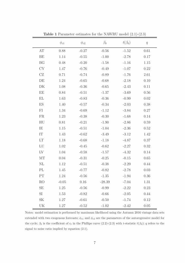
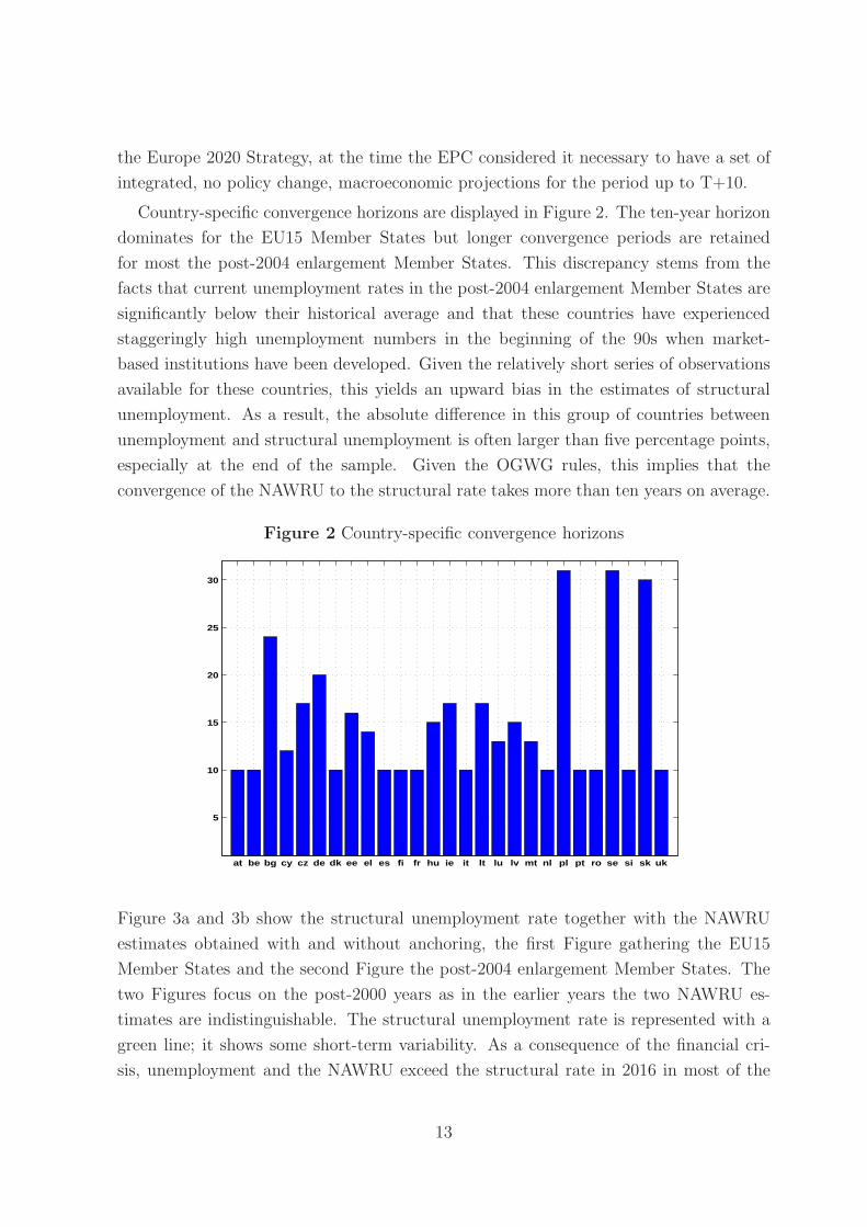
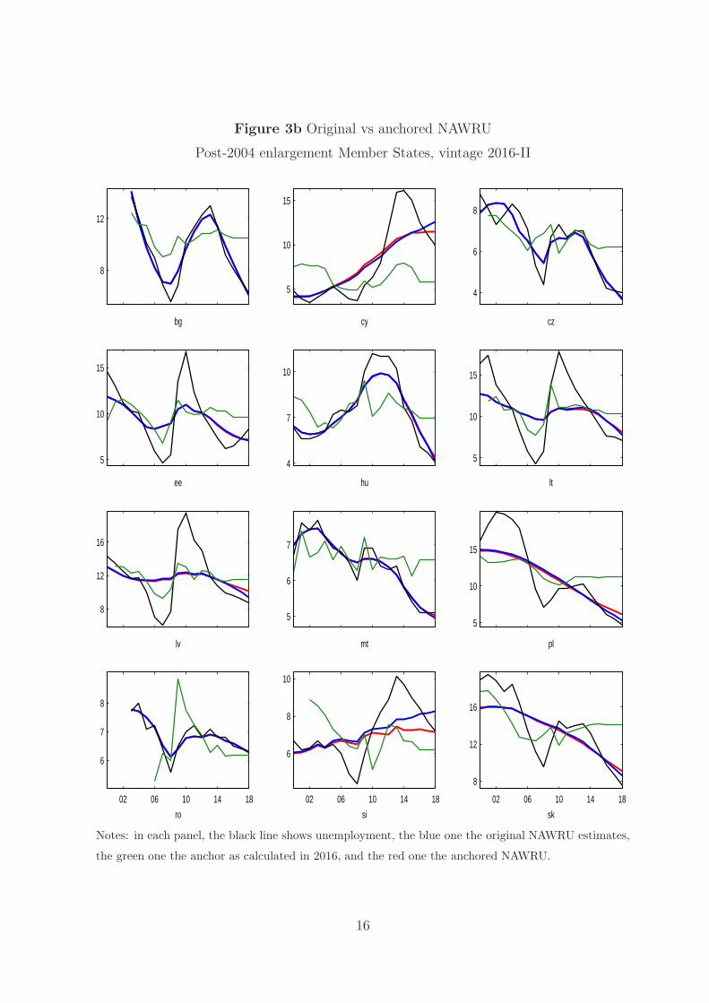
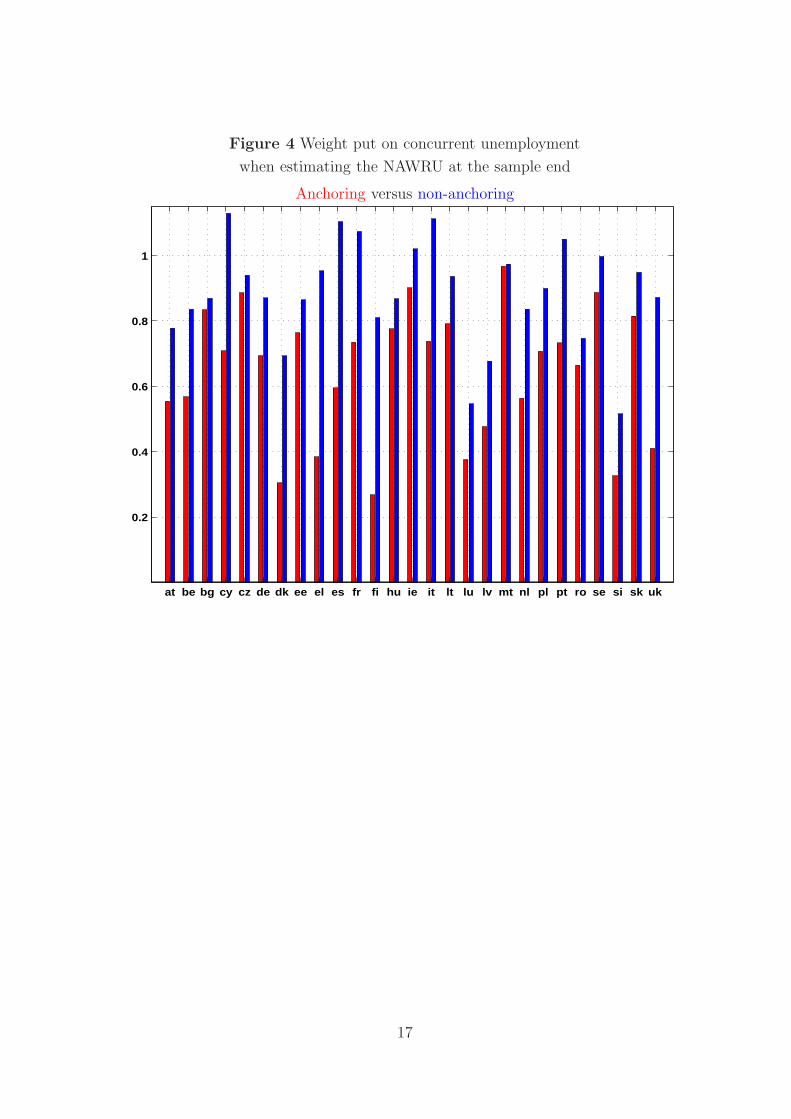
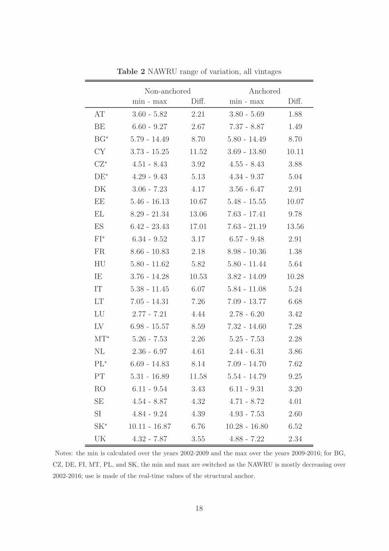
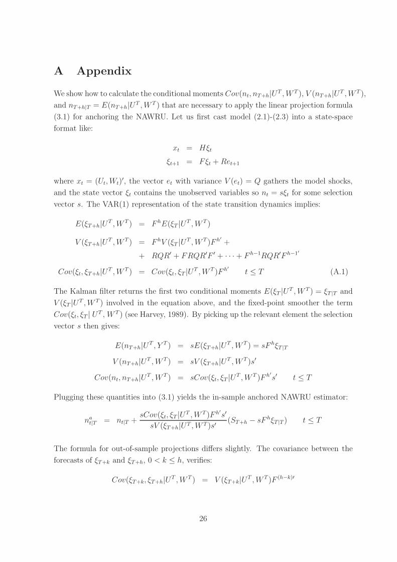
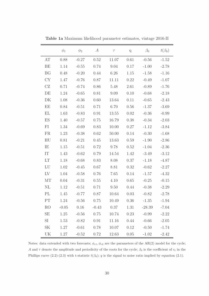

ISBN 978-92-79-64929-5
KC-BD-17-069-EN
-N
- Blank Page
-