Laboratory simulation of solar wind interaction with a

magnetic dipole field on lunar surface

by

Jia Han

University of Colorado at Boulder

A thesis submitted to the

Faculty of the Graduate School of the

University of Colorado in partial fulfillment

of the requirements for honors of

Bachelor of Arts

Department of Physics

2017

This thesis entitled:Laboratory simulation of solar wind interaction with a magnetic dipole field on lunar surface

written by Jia Hanhas been approved for the Department of Physics

Prof. Tobin Munsat

Prof. Paul Beale (Honors committee representative)

Prof. Mark Rast (Astrophysics department)

Date

The final copy of this thesis has been examined by the signatories, and we find that both thecontent and the form meet acceptable presentation standards of scholarly work in the above

mentioned discipline.

iii

Han, Jia (B. A. Physics)

Laboratory simulation of solar wind interaction with a magnetic dipole field on lunar surface

Thesis directed by Prof. Tobin Munsat

We perform laboratory experiments on the Colorado Solar Wind Experiment (CSWE) device

to study the dynamics of the solar wind interaction with lunar magnetic anomalies. A large cross-

section plasma flow with ion energies between 100 and 800 eV is incident on an insulating surface

embedded in a magnetic dipole field. Plasma is created by a Kaufman ion source under operating

pressure of 4×10−5 Torr. The beam profile has been characterized using a Langmuir probe and an

ion Energy Analyzer. The dipole field is created with a permanent magnet behind the surface. 2D

potential profiles are measured above the surface using an emissive Langmuir probe. With a dipole

moment perpendicular to the surface, the results show large positive potentials on the surface in the

dipole lobe regions, where the electrons are magnetically shielded while the unmagnetized ions go

to the surface. However, the magnitudes of these positive potentials follow the ion energies (in eV)

until 200 eV. Three possible explanations are investigated, including: (i) the electric field model,

(ii) secondary electron emission, (iii) surface material effect. This laboratory study will enhance

our knowledge on the lunar electric environment in the magnetic anomaly regions, which will help

us to understand the formation of the high-albedo swirl-shaped markers on the lunar surface.

iv

Acknowledgements

First, I would like to thank my advisor Prof. Tobin Munsat, for all his help on this thesis. I

really appreciated the opportunity he gave me to work in experimental plasma physics, and I really

learned a lot from him.

Next, I want to thank Dr. Xu Wang for his support on the research and the thesis. I am also

grateful to Dr. Zach Ulibarri and Dr. Li Hsia Yeo. It has been a great pleasure working on this

research project with all these people.

Last but not least, I would like to thank Prof. Tobin Munsat, Prof. Paul Beale and Prof.

Mark Rast, for serving on my thesis committee.

v

Contents

Chapter

1 Introduction and Background 1

1.1 Lunar Magnetic Anomalies . . . . . . . . . . . . . . . . . . . . . . . . . . . . . . . . 1

1.2 Solar Wind Interaction with Lunar Surface . . . . . . . . . . . . . . . . . . . . . . . 2

1.3 Lunar Swirls and Dust Transport . . . . . . . . . . . . . . . . . . . . . . . . . . . . . 4

2 Experiment Setup 7

2.1 The Colorado Solar Wind Experiment . . . . . . . . . . . . . . . . . . . . . . . . . . 7

2.1.1 Vacuum Chamber and Ion Source . . . . . . . . . . . . . . . . . . . . . . . . 8

2.1.2 Characterization of the simulated solar wind plasma . . . . . . . . . . . . . . 9

2.2 Simulating Solar Wind Interaction with Lunar Magnetic Anomalies . . . . . . . . . . 15

2.2.1 Plasma Parameters . . . . . . . . . . . . . . . . . . . . . . . . . . . . . . . . . 16

2.2.2 Emissive probe . . . . . . . . . . . . . . . . . . . . . . . . . . . . . . . . . . . 17

3 Results and Discussion 19

3.1 Surface Potential and Electric Field . . . . . . . . . . . . . . . . . . . . . . . . . . . 19

3.2 Surface Potential and Secondary Electron Emission . . . . . . . . . . . . . . . . . . . 24

3.3 Surface Potential and Surface Effects . . . . . . . . . . . . . . . . . . . . . . . . . . . 27

4 Conclusion 30

Bibliography 32

vi

Tables

Table

2.1 Comparison of parameters between lunar and laboratory conditions. . . . . . . . . . 16

vii

Figures

Figure

1.1 Lunar surface charging due to solar wind interaction . . . . . . . . . . . . . . . . . . 2

1.2 Surface potential in Gerasimovich magnetic anomaly . . . . . . . . . . . . . . . . . . 4

1.3 Result from previous laboratory experiment . . . . . . . . . . . . . . . . . . . . . . . 5

1.4 A picture of Lunar Swirl . . . . . . . . . . . . . . . . . . . . . . . . . . . . . . . . . . 5

2.1 CSWE chamber . . . . . . . . . . . . . . . . . . . . . . . . . . . . . . . . . . . . . . . 7

2.2 Schematic of the ion source . . . . . . . . . . . . . . . . . . . . . . . . . . . . . . . . 8

2.3 Photo of Langmuir probe and Energy Analyzer . . . . . . . . . . . . . . . . . . . . . 10

2.4 Circuit diagram and I-V curve of the Langmuir probe . . . . . . . . . . . . . . . . . 10

2.5 Electron Density . . . . . . . . . . . . . . . . . . . . . . . . . . . . . . . . . . . . . . 11

2.6 Energy analyzer diagram . . . . . . . . . . . . . . . . . . . . . . . . . . . . . . . . . . 12

2.7 Energy analyzer trace . . . . . . . . . . . . . . . . . . . . . . . . . . . . . . . . . . . 13

2.8 Ion Flux . . . . . . . . . . . . . . . . . . . . . . . . . . . . . . . . . . . . . . . . . . . 14

2.9 Experimental setup and trajectory of incoming plasma . . . . . . . . . . . . . . . . . 15

2.10 Emissive probe . . . . . . . . . . . . . . . . . . . . . . . . . . . . . . . . . . . . . . . 18

3.1 Surface potential contour at various ion energies . . . . . . . . . . . . . . . . . . . . 20

3.2 Maximum surface potential in the electron shielded region vs ion energy . . . . . . . 21

3.3 Potential along the z-axis with different ion energies . . . . . . . . . . . . . . . . . . 22

3.4 The ratio of Electric field force to Magnetic field force . . . . . . . . . . . . . . . . . 23

viii

3.5 Simulation results of electron trajectories . . . . . . . . . . . . . . . . . . . . . . . . 24

3.6 Surface potential contour at various ion currents . . . . . . . . . . . . . . . . . . . . 25

3.7 Potential along the z-axis with different ion currents . . . . . . . . . . . . . . . . . . 26

3.8 Surface potential for different materials . . . . . . . . . . . . . . . . . . . . . . . . . 28

Chapter 1

Introduction and Background

This thesis focuses on a laboratory experiment simulating solar wind interaction with a

magnetic dipole field. The experiment is conducted on the Colorado Solar Wind Experiment

(CSWE) device located at the Institute for Modeling Plasma, Atmospheres, and Cosmic Dust

(IMPACT) at the University of Colorado. A large cross-section flowing plasma with ion energies

between 100 eV and 800 eV is incident on an insulating surface embedded in a magnetic dipole field.

By studying the effect of plasma interaction with the magnetic dipole field, we will gain insight

on the lunar surface environment in the magnetic anomaly regions, especially information about

lunar surface charging. The surface charging in these magnetic anomaly regions may contribute

to electrostatic dust transport, which may be related to the formation of high albedo features on

lunar surface called “lunar swirls” [1].

1.1 Lunar Magnetic Anomalies

The magnetic field of Earth is known as geomagnetic field, which extends from the center

core to outer space. The shape of the field is similar to that of a magnetic dipole and its strength

at Earths surface ranges from 25-65 mT [4]. Unlike Earth, the moon does not have a global

magnetic field. Instead, it has localized crustal magnetic fields that are known as lunar magnetic

anomalies [5, 6, 18, 29]. Recent observations have measured that the surface magnetic field strength

in these anomaly regions are between 0.1 to 1000 nT [27], and their size ranges from less than 1

km to more than 100 km [12]. The theory behind the formation of magnetic anomalies remains

2

poorly understood. One hypothesis is that during large impact events, such magnetic field can be

generated on an airless bodies like the Moon [16]. This hypothesis is supported by the fact that

some of the highest crustal magnetization occurs at the antipodes of impact basins [20]. Regardless

of how they were formed, lunar magnetic anomalies can significantly effect the interaction between

the local plasma environment and the surface regolith.

1.2 Solar Wind Interaction with Lunar Surface

Because a global magnetic field is absent, direct interaction of solar wind plasma with lunar

surfaces are possible. Studies have shown different types of influences of solar wind plasma on

the lunar surface. As shown schematically in Fig 1.1, the dayside of the Moon can be positively

charged to few volts due to UV induced emission of photoelectrons [26]. On the nightside, in which

photoelectrons are absent, the formation of plasma wakes can charge the lunar surface negatively

to few hundreds of volts. Reflection and backscattering of solar wind ions also occur on the solar

wind upstream side of the Moon [22, 24].

Figure 1.1: Charging of the lunar surface due to solar wind interaction. [12, 10, 11]

3

Recently, in situ observations [11, 30, 21], computer simulations [13, 14, 15, 5], and laboratory

experiments [1] have indicated that the lunar crustal magnetic fields have a strong influence on the

solar wind plasma flow, possibly even forming mini-magnetospheres that prevent the solar wind

plasma from impinging on the surface.

At magnetic anomaly regions, solar wind electrons are generally magnetized while solar wind

ions remain weakly magnetized or unmagnetized. While the electrons are deflected and/or re-

flected, the ions do not feel a strong magnetic force and penetrate deeper or even reach the surface,

charging it positively. Futaana et al. [8] observed, using the remote energetic neutral atom imaging

technique, that the surface potential in Gerasimovich magnetic anomaly is larger than + 135 V

(Fig. 1.2). Based on conditions in this observation, Jarvinen et al. [19] developed a simulation, and

showed a result of +300 V surface potential in the Gerasimovich anomaly region. These findings

suggest that the surface charging on the dayside of the Moon is not solely governed by emission of

photoelectrons.

Previous laboratory investigations used flowing plasma with ion energies below 100 eV to

engulf a magnetic dipole field above an insulating surface. For dipole moment perpendicular to

the insulating surface (B⊥), results showed a large positive surface potential (close to ion flow

energies in eV) at dipole lobe regions (Fig. 1.3 a). The positive potential at the surface was due

to the accumulation of unmagnetized ions, where the electrons were magnetically excluded. The

electric potential exponentially decreases with distance from the surface on a Debye length scale.

For a dipole moment parallel to the insulating surface (B‖), there is no significant large positive

potential (Fig. 1.3 c) around the shielding regions. This is likely caused by the collisions between

mirror-trapped electrons and neutral particles [18]. In this thesis work, the plasma interaction with

the magnetic dipole fields was upgraded using a laboratory simulated solar wind plasma with the

ion flow energy up to 800 eV.

4

Figure 1.2: Surface potential in Gerasimovich magnetic anomaly. Blue lines are incoming solarwind protons. (a) shows deflection and engulfing the enhanced region without a change in velocity,(b) shows deceleration inside the magnetic anomaly due to the potential structure and (c) showsreflection in space before reaching the surface. [8]

1.3 Lunar Swirls and Dust Transport

Lunar swirls are regions on the lunar surface that have a high albedo, sinuous shape, and

appear optically immature (young regolith). Fig 1.4 shows a picture of the Reiner Gamma forma-

tion, an example of lunar swirls. The swirl is on the left of the picture next to the Reiner impact

crater. The swirl region with a oval shape and light color contrasts strongly against the dark surface

around it.

The lunar swirls are often found at regions with a relatively high magnetic field strength.

The reason for their formation remains a mystery. One possible model suggests that the deflection

of solar wind ion bombardment in lunar magnetic anomalies preserves long term space weathering

effects, which thus results in the formation of the lunar swirls [17]. Another model suggests that

the electric fields created due to charge separation in the magnetic anomaly regions may lead to

redistribution of electrostatically lofted fine-sized dust particles, which can be responsible for the

5

Figure 1.3: Result from previous laboratory experiment involving low ion flow energy. (a) & (c)are potential contour plots above the surface. (b) & (d) are the associate magnetic field strength.Figure (a), (b) are for B field perpendicular to the surface, where (c), (d) are for B field parallel tothe surface. [18]

Figure 1.4: The Reiner Gamma formation

surface albedo contrast in these regions [9].

By performing small-scale laboratory experiments of plasma interaction with a dipole field,

we will enhance our knowledge on the surface charging and electric field formation in magnetic

6

anomaly regions. This will help us to understand the lunar surface environment, and provide

insights on the formation of lunar swirls.

Chapter 2

Experiment Setup

2.1 The Colorado Solar Wind Experiment

The experiment was conducted using the Colorado Solar Wind Experiment (CSWE) device

[28]. The device uses a large cross-section Kaufman ion source with a plasma beam diameter of

12 cm, which can reach ion flow energies of 1.2 keV, and ion flow current density of 0.1 mA/cm2.

The chamber is typically operated at a pressure of 4 × 10−5 Torr, which is low enough so that

ion-neutral collisions are suppressed. A double Langmuir probe and an ion energy analyzer are

used to measure plasma characteristics, such as electron density or ion flux. They are mounted on

a two-dimensional translations stage, which can move the diagnostic instruments both along and

across the plasma flow.

Figure 2.1: Photo of the CSWE chamber. Plasma is created by ionizing gas from the left side ofthe chamber. A turbo pump is used in a differential pressure chamber right of the ion source toprevent gas build up in the experimental chamber. [28]

8

2.1.1 Vacuum Chamber and Ion Source

The experimental vacuum chamber is 183 cm in length and 76 cm in diameter. Fig 2.1 shows

a photo of the CSWE vacuum chamber, where plasma is generated on the left and flows to the

right into the chamber.

Plasma is generated using a high-current Kaufman KDC 100 ion source. As gas flows into the

ion source, molecules are singly ionized by the energetic electrons emitted from a heated cathode.

The ions are then accelerated into the chamber by an anode grid, where the ion energy is determined

by the anode potential. The ion beam at the exit of the source is 12 cm in diameter and diverges

at 7 degrees by the ion optics to create a large uniformity. The flowing plasma is maintained at

quasi-neutrality by using a neutralizing filament at the end of the source. A controlled number of

electrons are emitted from the neutralizer, so that the density of electrons in the ion beam matches

the density of the ions approximately. A schematic of the ion source is shown in Fig 2.2.

Figure 2.2: A schematic of the Kaufman KDC 100 ion source. Gas molecules are ionized at thecathode. The anode potential with respect to ground selects the ion energy. A two grid ion opticdesign is used to shape the ion beam. The neutralizer at the end of the source is used to maintainthe plasma’s neutrality.

9

As pressure increases with gas flowing into the chamber, collisional effect need to be taken into

consideration. To avoid charge exchange between ions and neutral atoms, we use a turbo molecular

pump located in a differential pressure chamber (right side on Fig 2.1), so that the neutral gas

flow is partially isolated from the rest of the chamber. The base pressure of the vacuum chamber

without the plasma source operating is maintained at 3×10−7 Torr, and is at 4×10−5 Torr during

plasma flows.

We have tested the ion source with hydrogen, nitrogen, and argon gases. Although hydrogen

is the best representative of solar wind, it does not work very well in laboratory environment. With

the small ionization cross-section, hydrogen requires a higher gas flow rate in order to reach the

desired ion current. This increases the operating pressure of the chamber, which makes it hard to

eliminate charge-exchange collisions. On the other hand, nitrogen and argon can be easily ionized

at the relatively low operating pressure described above. Since nitrogen has a smaller mass number

than argon, we have used nitrogen for the experiment described in this thesis. General physics

results can be then interpreted for actual solar wind constituents as needed.

2.1.2 Characterization of the simulated solar wind plasma

2.1.2.1 Langmuir Probe

A double planar Langmuir probe is used to determine the plasma potential, electron density,

and electron temperature. A picture of the Langmuir probe is shown on the left of Fig 2.3. The

probe consisting of two tantalum discs with a diameter of 6.35 mm [28], is inserted into plasma

and biased with respect to the plasma potential (Vp). A current voltage (I-V) characteristic (Fig.

2.4 b) is measured as the applied bias voltage (Vbias) sweep from negative to positive. The probe

collects a saturated ion current curve when Vbias is sufficiently negative with respect to Vp. The ion

collecting process continues until Vbias reaches Vp, where ions start to get repelled from the probe.

The electron current is collected and all ions are repelled from the probe when Vbias >> Vp. Fig

2.4 (a) shows a schematic diagram of a Langmuir probe circuitry. The current is determined by

10

Figure 2.3: A photo of the diagnostic equipment and the 2-dimensional stage for in-vacuum transla-tion. On the left of the stage is a double planar Langmuir probe, and on the right is an ion energyanalyzer. The translation stage is able to move across the chamber in two directions. Duringnormal operation, plasma would be flowing from the lower-left corner of the photo.

measuring the voltage across resistor R as the probe’s bias potential changes [23].

(a) Circuit diagram

-60 -40 -20 0 20 40-0.2

0.0

0.2

0.3

0.5

0.7

0.9

1.0

Nor

mal

ized

Cur

rent

(I)

Potential (V)

Sample Langmuir Probe trace

Ion Saturation

ElectronSaturation

(b) Sample I-V curve

Figure 2.4: (a) A simple circuit diagram of the Langmuir probe. The I-V characteristic of theplasma is obtained by sweeping an applied bias voltage across the probe. The current across theresistor R gives the current passing through the probe. (b) A sample Langmuir probe trace showingthe I-V characteristics for the plasma. Ion or electron current is collected according to the biasvoltage compared to the plasma potential. This curve is used to determine the plasma potential,electron density, and electron temperature. [23]

11

From the current-voltage (I-V) characteristics, we observed two Maxwellian distributions

of electrons: one at a higher temperature, and one at a lower temperature. The hot electron

population has a temperature around 10 eV, while the cold electrons are around 0.5 eV. The hot

electron population has a density that is approximately 1% of the cold population.

The electron density of the plasma is also determined from the I-V characteristics, and the

results are shown in Fig 2.5. We diagnose the plasma characteristics at three different ion energies,

and each corresponds to three different ion currents. The three plots on the left of Fig 2.5 show

the electron density vs. position across the x-axis, which is the horizontal displacement from the

beam’s center axis. Three plots on the right shows measurements taken along the z-axis, which is

the displacement along the beam’s axis. The electron density plots are for 200 eV, 400 eV, and 800

eV from bottom to top, and black/blue/red curve shows result for 20/40/80 mA, respectively.

Figure 2.5: Plot of electron densities that are analyzed from Langmiur probe measurements. X-position is the horizontal displacement from the beam’s center axis. Z-position is the distance alongthe beam axis. The green region represents positions dedicated for performing experiments. [28]

12

2.1.2.2 Ion Energy Analyzer

Figure 2.6: Top: Sketch of the energy analyzer geometry.Bottom: Potentials of the grids along the axis of the plasma beam. [3]

An ion energy analyzer (on the right of Fig 2.3) is used to determine the ion energy and ion

flux. The device measures the energy distribution of ions in plasma using a retarding electrostatic

field. In the CSWE diagnostic, we use a plane four-grid retarding-field electrostatic analyzer. Fig

2.6 shows a schematic diagram for it. The energy analyzer consists of four square grids, with grid

No. 0 facing the incoming plasma, and the last grid on the right is the collector grid [3]. As charged

particles enter grid No. 0, the ions are accelerated towards grid No. 1, which is held at a negative

potential (-55 V), and the electrons are repelled by grid No. 1. After their entrance, the ions are

13

selected based on their kinetic energy by the retarding potential field between grid No. 1 and No.

2. Grid No. 2 creates a potential barrier for the ions by sweeping from 0 V to + 1000 V. Ions with

kinetic energies larger than the potential of grid No. 2 will eventually reach the collector grid. We

measure the ion current at the collector grid as a function of the sweeping voltage on grid No. 2.

When the ions reach the collector grid, they can induce secondary electrons. The potential of grid

No. 3 is chosen to be held at -85 V, so that the potential difference between it and the collector

grid is greater than the kinetic energy of the secondary electrons. This will prevent them escaping

from the collector grid.

0 100 200 300 400 500 600 700 800 900Retarding Potential (V)

0.0

0.2

0.4

0.6

0.8

1.0

1.2

1.4

Norm

aliz

ed V

alue

s

Current, I dI/dV200 V400 V800 V

200 V400 V800 V

Normalized Energy Analyzer Sample Traces and Derivatives

Figure 2.7: A sample trace of the Ion Energy Analyzer. The solid lines are the energy analyzertrace, and the dotted lines are their derivatives. The width of the peaks in the derivative tracesindicates the thermal energy spread. The sharp drop off at each specific energy levels indicate thatthe plasma is mono-energetic. [28]

Figure 2.7 shows a sample measurement taken from the Ion Energy Analyzer. The sharp drop

off at specific energies indicates the plasma ion energies, showing that the plasma flow is mono-

energetic. The small drop off (near 10 eV) before the sharp step indicates a production of thermal

ions due to charge-exchange collision effects. Although the thermal ions is small compare to the

ion population flowing out from the source, they are not negligible. However, for the experiment

described in this thesis, we are mostly interested on the electron population instead of the ions.

14

Therefore, the effect of thermal ion production is unlikely to contribute a difference in the result.

Figure 2.8: Plot of ion flux calculated from measurements of the Ion Energy Analyzer. X-positionis the horizontal placement from the beam’s center axis. Z-position is the distance from the source.The green region are positions dedicated for taking future measurements. [28]

Figure 2.8 shows the ion flux of the simulated solar wind plasma. Over the region where

experiments are performed (green region), the ion flux is proportional to the source current. The

density and flux are maximum at the center of the beam, and drops up to 30% around the edge

of the green region. The ion source behaves as expected, except for ion flow with 200eV and 80

mA. The ion flux for this particular combination of ion energy and current does not double that

of 40 mA. This is because the source’s ion optics are not designed to supply large currents at

high voltages. Thus, even with a higher current supplied to the acceleration grids, not all ions are

allowed to flow into the chamber due to the low ion energy constraint. Similarly, the 800 V and 80

mA ion beam suggests an ion flux of more than double in magnitude than the 40 mA beam. This is

likely caused by the increase in performance of the ion optics from the source. For the experiment

15

described in this thesis, we will only be operating with ion flow energy and current combinations

that behaves more as expected. Therefore, although the ion current does not scale in some cases,

it is not a major concern in this experiment.

2.2 Simulating Solar Wind Interaction with Lunar Magnetic Anomalies

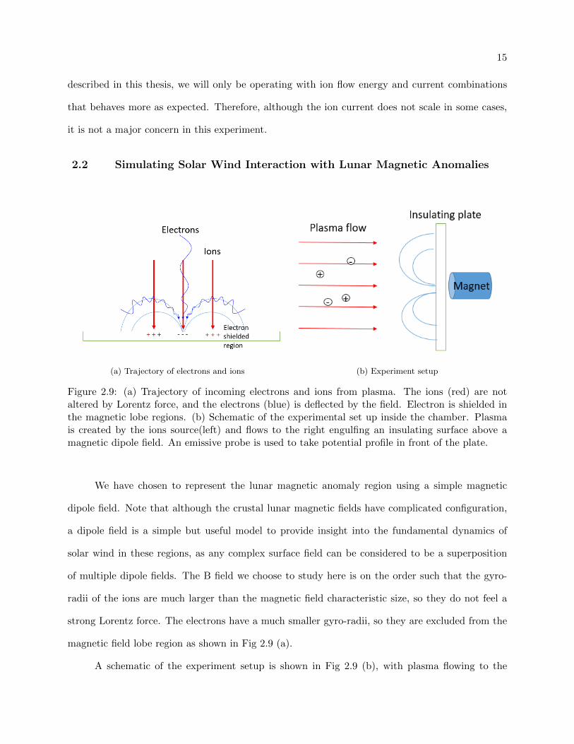
(a) Trajectory of electrons and ions (b) Experiment setup

Figure 2.9: (a) Trajectory of incoming electrons and ions from plasma. The ions (red) are notaltered by Lorentz force, and the electrons (blue) is deflected by the field. Electron is shielded inthe magnetic lobe regions. (b) Schematic of the experimental set up inside the chamber. Plasmais created by the ions source(left) and flows to the right engulfing an insulating surface above amagnetic dipole field. An emissive probe is used to take potential profile in front of the plate.

We have chosen to represent the lunar magnetic anomaly region using a simple magnetic

dipole field. Note that although the crustal lunar magnetic fields have complicated configuration,

a dipole field is a simple but useful model to provide insight into the fundamental dynamics of

solar wind in these regions, as any complex surface field can be considered to be a superposition

of multiple dipole fields. The B field we choose to study here is on the order such that the gyro-

radii of the ions are much larger than the magnetic field characteristic size, so they do not feel a

strong Lorentz force. The electrons have a much smaller gyro-radii, so they are excluded from the

magnetic field lobe region as shown in Fig 2.9 (a).

A schematic of the experiment setup is shown in Fig 2.9 (b), with plasma flowing to the

16

right, where a 30 × 30 square insulating plate is positioned. The insulating plate is 56 cm away

from the ion source. The ion source creates a flowing plasma with the ion energy between 100-800

eV, and the ion current of 1-100 mA. The electron density of the plasma flow at the plate’s region

is 1.14 × 106 − 108cm−3, and the electron temperature is about 0.5 eV (cold electrons dominate).

The magnetic dipole field is created using a permanent magnet sitting behind the insulating plate.

The maximum magnetic field strength is about 580G at the surface. An emissive probe is used to

measure the 2D potential profile in front of the plate.

2.2.1 Plasma Parameters

Laboratory Lunar Case (Strong |B |region)

Ion Species N+2 H+

Ion Mach Number, Vi√Ti/Tm

11 9

Ion Flow Energy, Eb(eV ) 100 - 800 1000

Electron Temperature, Te 0.5 eV (cold) / 10 eV (hot) 10 eV

Ion Temperature, Ti 10 eV 14 eV

Ion Mach Number, M 11 9

Electron Gyro-ratio, re/L < 1 (0.3 cm / 2 cm) << 1 (0.35 km / 30 km)

Ion Gyro-ratio, ri/L >> 1 (250-720 cm / 2cm) > 1 (150 km / 30 km)

Electron Debye Ratio, λDe/L < 1 (0.2 cm / 2 cm) << 1 (0.01 cm / 30 km)

Ion Debye Ratio, λDi/L < or > 1 (1.4-6.5 cm / 2 cm) << 1 (0.1 km / 30 km)

Table 2.1: Comparison of parameters between lunar and laboratory conditions.

A comparison of plasma parameters between space and laboratory conditions is summarized

in Table 2.1. The reason of using nitrogen instead of hydrogen as the ion species is explained earlier

in this chapter. Although the nitrogen molecular mass is heavier than the hydrogen, the ion Mach

number (ratio of ion flow speed to ion sound speed) is much larger than 1 in both the laboratory

and lunar cases. This indicates that both cases have a supersonic ion flow speed. The CSWE

creates a flowing plasma with the ion energy up to 1 keV, close to a typical solar wind energy of

1.2 keV. The solar wind electron density and temperature are 10 cm3 and 10 eV, respectively.

The magnetic fields characteristic size (L) is defined as the distance between the surface and

the position where the magnetic field strength has significantly dropped. For the magnetic field

17

strength that we have chosen, the electron gyro-ratio is less than 1, and the ion gyro-ratio is greater

than 1 for both lunar and laboratory cases. This means that the electrons are magnetized, while

the ions remain unmagnetized. The ion Debye length is calculated using the equation

λD =

√ε0Ei

ne2(2.1)

where Ei is the ion energy, and n is the electron density. We are able to adjust the ion Debye length

by shooting plasma with different ion energies. Therefore, the ion Debye ratio can be greater or

less than 1 in the laboratory environment. It is impossible to reproduce the absolute scale of solar

wind interactions with the lunar surface in laboratory environment. However, the dimensionless

parameters in the laboratory case match the condition of lunar magnetic anomaly regions with

magnetic field strength of 30 nT at 30 km altitude [16, 21].

2.2.2 Emissive probe

We use an emissive Langmuir probe to measure the potentials in front of the insulating

surface with the current-voltage method. The Emissive probe is an example of electron-emitting

probe that can measure the characteristics of the plasma. During operation, the probe emits

thermionic electrons by heating a filament in addition to collecting electrons and ions from the

plasma. At a specific electron emission current (Ib), the probe bias potential indicates the local

plasma potential (Vp). Therefore, we can make the probe potential equal the local plasma potential

(Vp) by externally biasing the current to (Ib). This is called the current voltage method. The

Emissive probe has an advantage comparing to other probes, as it provides a direct measurement

of the potential without requiring a voltage sweep or data reduction.

The probe consists a tungsten filament of approximately 1 cm long and 0.025 mm in diameter.

It is spot welded to two nickel supporting wires, and the wires are protected in a ceramic tubes

from plasma (Fig 2.10). We measure the voltage across the probe at a feedback current of 1 µA.

This feedback current is associated with an electron emission current of 10 µA. The above values

are chosen from calibrations with an inflection-point method [25]. We move the emissive probe

18

using the 2D motorized translation stage shown in Fig 2.3, and measure the 2D potential contour

in front of the insulating surface over a magnetic dipole field.

Figure 2.10: Construction of the Emissive probe [25]

Chapter 3

Results and Discussion

3.1 Surface Potential and Electric Field

With a perpendicular magnetic dipole moment, Fig 3.1 shows the potential contours for 100

eV, 200 eV, 400 eV, and 800 eV ion flow energies. In the cusp regions, neutral plasma reaches the

surface without deflection, therefore potentials are measured to be close to 0 V. In the lobe regions,

electrons are deflected by the magnetic field, while ions reach the surface, forming an electron-

shielded region with positive potentials near the insulating surface. In the absence of other effects,

it is expected that the potential should build up to the ion energy.

For the 100 eV and 200 eV cases (Fig. 3.1 a,b), potentials at 3 mm above the surface are

measured to be around +90 V and +180 V, respectively. The asymmetry in potential distributions

is likely caused by the movement of probe that is not perfectly parallel to the surface. The electrons

were magnetized, and thus they were prohibited from entering the dipole lobe regions. The ions

are not magnetized, so they can easily travel through the magnetic field lines, charging the surface

positively. For the 400 eV and 800 eV cases (Fig. 3.1 c,d), the maximum potential above the

surface is around +230 V and +170 V, respectively. The surface potentials are still positive, but

their magnitudes are much smaller than the ion flow energies. The electron-shielded region extends

1.5-3.5 cm above the surface, for 100-800 eV respectively. The basic shape and magnitude of these

surface contours is largely consistent with the basic physical picture of magnetic electron shielding.

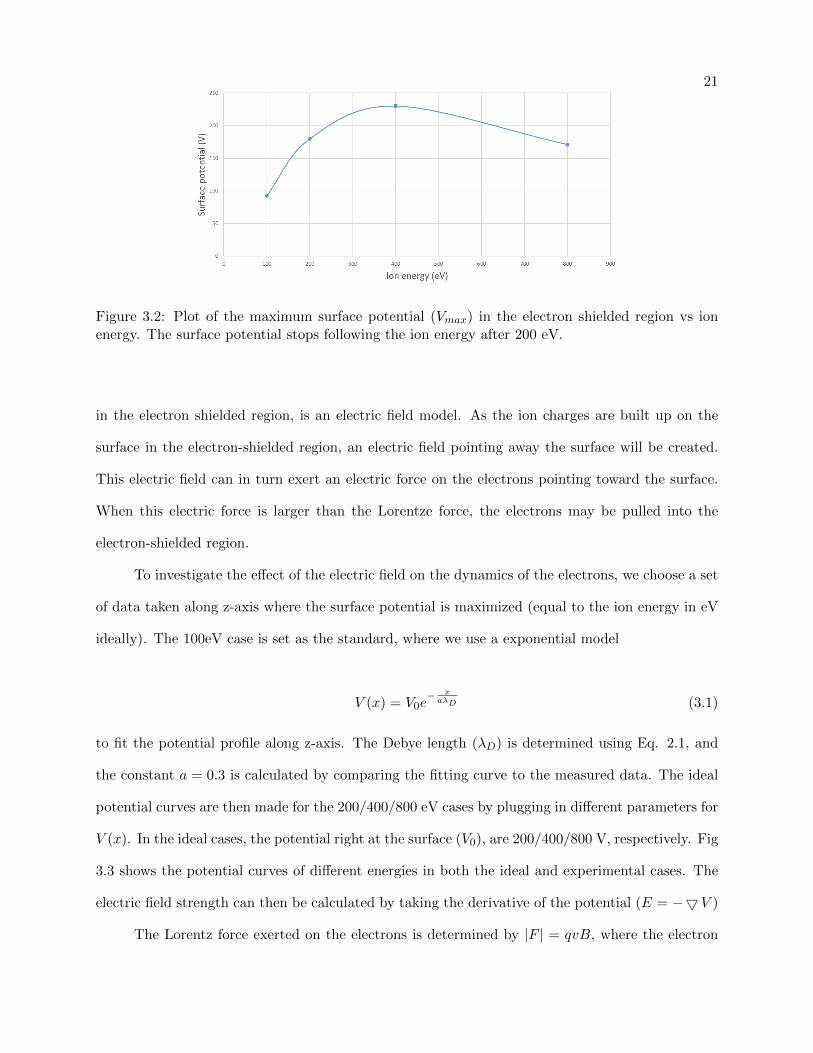
A major unexpected result from these observations is that the measured surface potential

stops following the ion flow energy after 200 eV in the electron shielded region. Fig 3.2 shows the

20

(a) 100 eV (b) 200 eV

(c) 400 eV (d) 800 eV

Figure 3.1: Potential contours above the surface. The ion flow energies are respectively: (a) 100eV,(b) 200eV, (c) 400eV, and (d) 800eV. The ion flow current for all energies is 5 mA. The x-axis isparallel to the surface and z-axis is perpendicular to the surface. The asymmetries of the potentialare likely due to the asymmetry of the ion source.

maximum surface potential plotted vs. ion energy. At low ion energies, there is a linear relationship,

but the curve levels off and even rolls over to negative slope at the highest ion energies. This

indicates that either part of the ion density failed to reach the surface, or the electron shielding

from the magnetic field is incomplete. Since ions are much heavier than electrons, we suspect that

the electrons are much more likely to be influenced than the ions.

One possible explanation of this drop, where part of the electron population might reach the surface

21

Figure 3.2: Plot of the maximum surface potential (Vmax) in the electron shielded region vs ionenergy. The surface potential stops following the ion energy after 200 eV.

in the electron shielded region, is an electric field model. As the ion charges are built up on the

surface in the electron-shielded region, an electric field pointing away the surface will be created.

This electric field can in turn exert an electric force on the electrons pointing toward the surface.

When this electric force is larger than the Lorentze force, the electrons may be pulled into the

electron-shielded region.

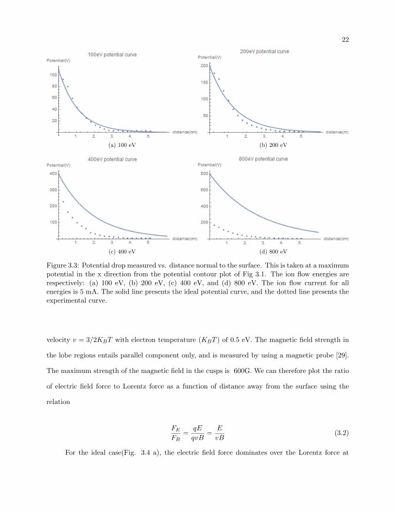
To investigate the effect of the electric field on the dynamics of the electrons, we choose a set

of data taken along z-axis where the surface potential is maximized (equal to the ion energy in eV

ideally). The 100eV case is set as the standard, where we use a exponential model

V (x) = V0e− xaλD (3.1)

to fit the potential profile along z-axis. The Debye length (λD) is determined using Eq. 2.1, and

the constant a = 0.3 is calculated by comparing the fitting curve to the measured data. The ideal

potential curves are then made for the 200/400/800 eV cases by plugging in different parameters for

V (x). In the ideal cases, the potential right at the surface (V0), are 200/400/800 V, respectively. Fig

3.3 shows the potential curves of different energies in both the ideal and experimental cases. The

electric field strength can then be calculated by taking the derivative of the potential (E = −5V )

The Lorentz force exerted on the electrons is determined by |F | = qvB, where the electron

22

(a) 100 eV (b) 200 eV

(c) 400 eV (d) 800 eV

Figure 3.3: Potential drop measured vs. distance normal to the surface. This is taken at a maximumpotential in the x direction from the potential contour plot of Fig 3.1. The ion flow energies arerespectively: (a) 100 eV, (b) 200 eV, (c) 400 eV, and (d) 800 eV. The ion flow current for allenergies is 5 mA. The solid line presents the ideal potential curve, and the dotted line presents theexperimental curve.

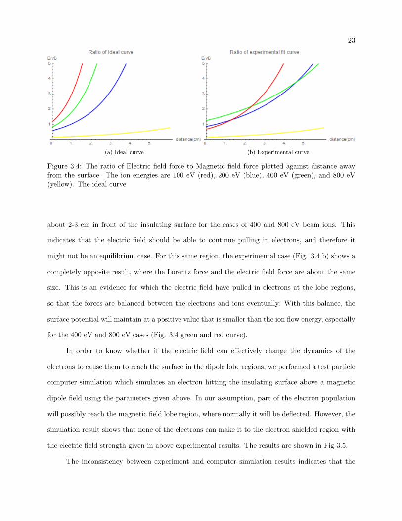
velocity v = 3/2KBT with electron temperature (KBT ) of 0.5 eV. The magnetic field strength in

the lobe regions entails parallel component only, and is measured by using a magnetic probe [29].

The maximum strength of the magnetic field in the cusps is 600G. We can therefore plot the ratio

of electric field force to Lorentz force as a function of distance away from the surface using the

relation

FE

FB=

qE

qvB=

E

vB(3.2)

For the ideal case(Fig. 3.4 a), the electric field force dominates over the Lorentz force at

23

(a) Ideal curve (b) Experimental curve

Figure 3.4: The ratio of Electric field force to Magnetic field force plotted against distance awayfrom the surface. The ion energies are 100 eV (red), 200 eV (blue), 400 eV (green), and 800 eV(yellow). The ideal curve

about 2-3 cm in front of the insulating surface for the cases of 400 and 800 eV beam ions. This

indicates that the electric field should be able to continue pulling in electrons, and therefore it

might not be an equilibrium case. For this same region, the experimental case (Fig. 3.4 b) shows a

completely opposite result, where the Lorentz force and the electric field force are about the same

size. This is an evidence for which the electric field have pulled in electrons at the lobe regions,

so that the forces are balanced between the electrons and ions eventually. With this balance, the

surface potential will maintain at a positive value that is smaller than the ion flow energy, especially

for the 400 eV and 800 eV cases (Fig. 3.4 green and red curve).

In order to know whether if the electric field can effectively change the dynamics of the

electrons to cause them to reach the surface in the dipole lobe regions, we performed a test particle

computer simulation which simulates an electron hitting the insulating surface above a magnetic

dipole field using the parameters given above. In our assumption, part of the electron population

will possibly reach the magnetic field lobe region, where normally it will be deflected. However, the

simulation result shows that none of the electrons can make it to the electron shielded region with

the electric field strength given in above experimental results. The results are shown in Fig 3.5.

The inconsistency between experiment and computer simulation results indicates that the

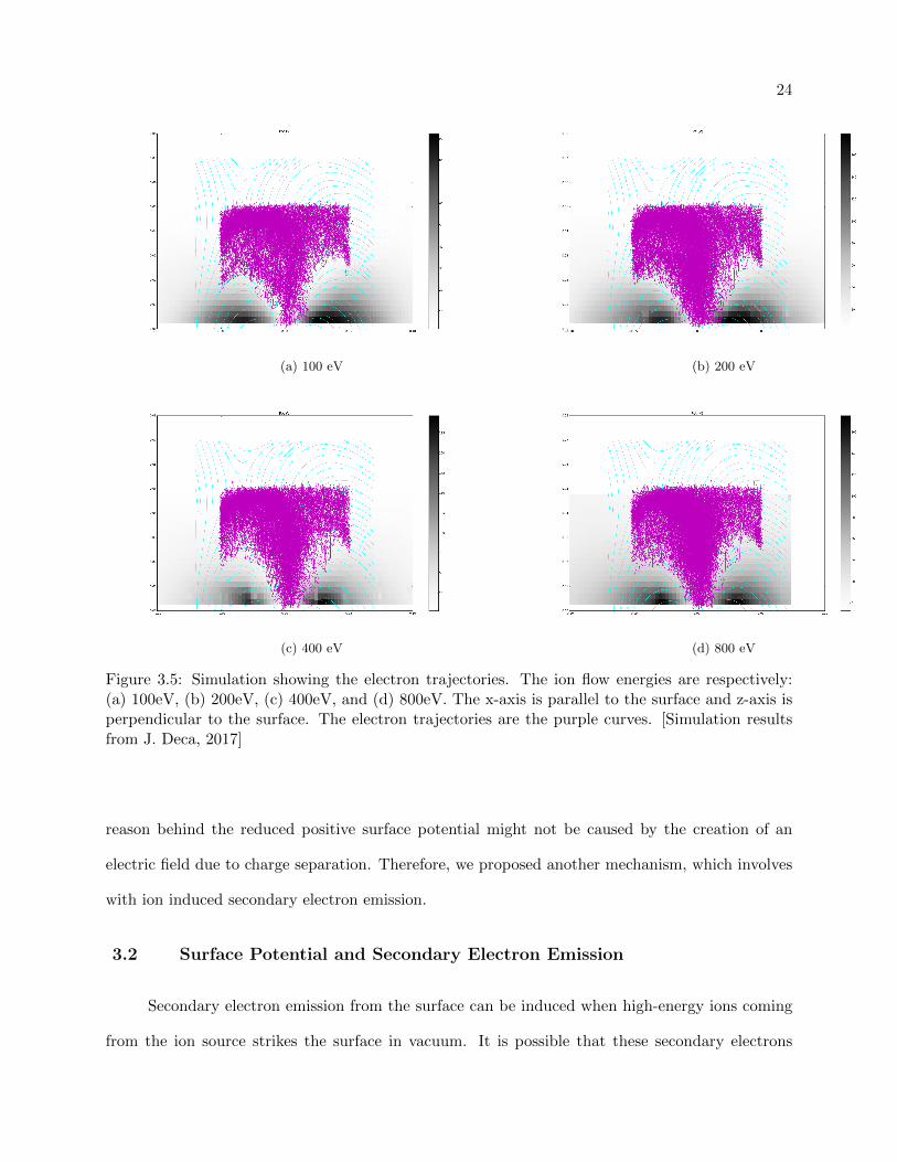
24

(a) 100 eV (b) 200 eV

(c) 400 eV (d) 800 eV

Figure 3.5: Simulation showing the electron trajectories. The ion flow energies are respectively:(a) 100eV, (b) 200eV, (c) 400eV, and (d) 800eV. The x-axis is parallel to the surface and z-axis isperpendicular to the surface. The electron trajectories are the purple curves. [Simulation resultsfrom J. Deca, 2017]

reason behind the reduced positive surface potential might not be caused by the creation of an

electric field due to charge separation. Therefore, we proposed another mechanism, which involves

with ion induced secondary electron emission.

3.2 Surface Potential and Secondary Electron Emission

Secondary electron emission from the surface can be induced when high-energy ions coming

from the ion source strikes the surface in vacuum. It is possible that these secondary electrons

25

are attracted by the positive surface potential in the electron shielded region, and get pulled into

it. To eliminate the effect due to secondary electrons, all measurements we took in the previous

section are at a plasma ion current of 5 mA. With a lower ion current, we expect secondary electron

emissions less likely to take place.

-5 -3 0 3 5 8

1

2

3

4

5

x (cm)

z (c

m)

2.500

21.63

40.75

59.88

79.00

98.13

117.2

136.4

155.5

Potential (V)

(a) 1 mA

-10 -5 0 5 10 15

1

2

3

4

5

X (cm)

Z (c

m)

2.000

32.63

63.25

93.88

124.5

155.1

185.8

216.4

247.0

Potential (V)

(b) 5 mA

-5.5 -3.0 -0.5 2.0 4.5 7.0

1

2

3

4

5

X (cm)

Z (c

m)

1.000

35.63

70.25

104.9

139.5

174.1

208.8

243.4

278.0

Potential (V)

(c) 100 mA

Figure 3.6: Potential contours above the surface.The ion currents are respectively: (a) 1 mA, (b) 5 mA, (c) 100 mA. The ion flow energy for allcurrents is 400 eV. The x-axis is parallel to the surface and z-axis is perpendicular to the surface.The asymmetries of the potential are likely due to the asymmetry of the ion source.

In order to acquire a better understanding on this effect, we took measurements at higher ion

currents with the same ion energy. Since the ion velocity was constraint, the ion density increases

26

to reach a higher ion current. Fig 3.6 is the resulting 2D potential contours with all measurements

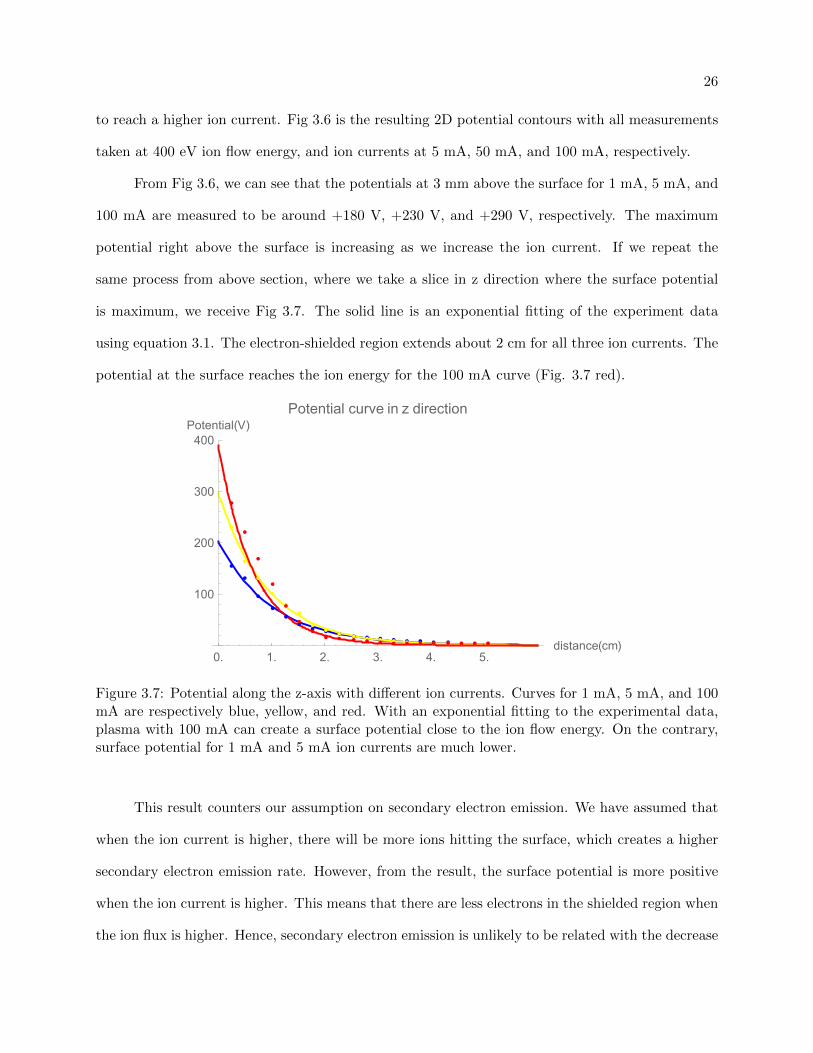
taken at 400 eV ion flow energy, and ion currents at 5 mA, 50 mA, and 100 mA, respectively.

From Fig 3.6, we can see that the potentials at 3 mm above the surface for 1 mA, 5 mA, and

100 mA are measured to be around +180 V, +230 V, and +290 V, respectively. The maximum

potential right above the surface is increasing as we increase the ion current. If we repeat the

same process from above section, where we take a slice in z direction where the surface potential

is maximum, we receive Fig 3.7. The solid line is an exponential fitting of the experiment data

using equation 3.1. The electron-shielded region extends about 2 cm for all three ion currents. The

potential at the surface reaches the ion energy for the 100 mA curve (Fig. 3.7 red).

0. 1. 2. 3. 4. 5.distance(cm)

100

200

300

400Potential(V)

Potential curve in z direction

Figure 3.7: Potential along the z-axis with different ion currents. Curves for 1 mA, 5 mA, and 100mA are respectively blue, yellow, and red. With an exponential fitting to the experimental data,plasma with 100 mA can create a surface potential close to the ion flow energy. On the contrary,surface potential for 1 mA and 5 mA ion currents are much lower.

This result counters our assumption on secondary electron emission. We have assumed that

when the ion current is higher, there will be more ions hitting the surface, which creates a higher

secondary electron emission rate. However, from the result, the surface potential is more positive

when the ion current is higher. This means that there are less electrons in the shielded region when

the ion flux is higher. Hence, secondary electron emission is unlikely to be related with the decrease

27

in surface potential.

3.3 Surface Potential and Surface Effects

With the inconsistency between experiment and simulation described above, and based on

the negative slope in Fig. 3.2 at high ion energies, we begin to suspect whether the decrease in

surface potential is affected by the material of the surface. For both results in section 3.1 and 3.2, we

have used a plexiglass plate as the insulating surface. Although it is a non-conducting surface, ion

bombardment will have the ability to create a surface conductivity. The plexiglass has a thickness

of 2 mm. Thus, it is possible that the plasma interaction does not effect the interior conductivity,

but only changes the surface conductivity of the plexiglass material. Ion bombardment may also

lead to the sputtering of atoms from the surface that may collide with the main ion beam and/or

secondary electrons, which results in electron scattering into magnetic lobe regions.

To investigate more on the surface effect, we replaced the insulating surface with two other

materials and measured the surface potentials across the x-axis in front of the plate, so that the

positive potential in electron shielded region is at maximum. The materials we used are glass and

alumina. The glass plate has the same length as the plexiglass plate (30 cm) and with a thickness of

1 mm. The alumina plate consist a high density fiber based ceramic material with alumina purity

greater than 99%. A general comparison between the surface potential for different materials is

shown in Fig 3.8.

As shown in Fig 3.8, the surface potential varied with the material we chose for the insulating

surface. For both glass and alumina material, we observe a lower surface potential compared to

the plexiglass material we had in section 3.1 and 3.2. For ion flow energy of 100 eV (Fig. 3.8

a), the maximum potential at the surface (Vmax) for alumina, glass, and plexiglass are +65 V,

+80 V, and +95 V, respectively. Vmax for alumina is about 20 % lower than that of plexiglass.

For 200 eV case (Fig. 3.8 b), Vmax for alumina, glass, and plexiglass became +100 V, +80 V,

and +180 V, respectively. Different from ion energy of 100 eV case, Vmax for glass material was

lower than that of alumina in the 200 eV case. For 400 eV case, Vmax of plexiglass (+200 V) is

28

0 5 10 15 20 25 30 35

0

20

40

60

80

100Po

tent

ial (

V)

X (cm)

Alumina Glass Plexiglass

(a) 100 eV

0 5 10 15 20 25 30 35

0

20

40

60

80

100

120

140

160

180

200

Pote

ntia

l (V)

X (cm)

Alumina Glass Plexiglass

(b) 200 eV

0 5 10 15 20 25 30 35

0

50

100

150

200

Pote

ntia

l (V)

X (cm)

Alumina Glass Plexiglass

(c) 400 eV

Figure 3.8: Surface potential measuring along the x-axis in front of the surface.The ion flow energies are respectively: (a) 100eV, (b) 200eV, and (c) 400eV.

about twice that of glass (+70 V) and alumina (+100 V). The difference between surface potentials

becomes more significant as the ion flow energy increases. In section 3.1, we found that the surface

potential diverges from the ion flow energy more as we increase the ion energy (Fig. 3.2). The

switch of surface material revealing a larger change in Vmax indicates that using different material

of insulating surface is likely to be a contributing factor to the observed differences between ion

flow energy and maximum surface potential. The interaction of plasma with the insulating surface

might change the surface conductivity, and create a surface charging effect.

29

Another interesting feature apparent in Fig 3.8 is the asymmetry between two peaks on the

potential plot. The two maximum positions correspond to two lobe regions of the magnetic dipole.

When we performed the experiments in section 3.1 and 3.2, we suspected that the asymmetry was

caused by asymmetry in electron density and ion flux of the ion source (Figs. 2.5 & 2.8). However,

as we switched to a different material, the asymmetry changed and grew larger. For plexiglass, the

first potential peak is lower than the second peak, whereas for glass and alumina, it is the opposite.

The alumina plate also showed a less smooth potential curve than the two other materials. While

we observed the various changes occurred with surface material, we were still unsure about the

pattern and reason of these changes.

Further experiments will be performed to gain more information on the surface material effect.

We are currently building a spherical Langmuir probe to exterminate the density of electrons in

the shielded region in front of the insulating surface. Since the planer Langmuir probe we had used

previously only detects electron current in two directions, it does not perform best in the presence

of a magnetic field where electrons gyrate in the direction of the field lines. By using a spherical

probe, we hope to determine whether the decrease in surface potential is caused by unexpected

electron population.

Chapter 4

Conclusion

We performed laboratory simulations of solar wind plasma interaction with a magnetic dipole

field on an insulating surface. For ion energies below 200 eV, the results are consistent with a simple

model based on preferential magnetic shielding of beam electrons (but not ions), where the surface

potential is close to the ion flow energy. However, for 400 eV and 800 eV cases, the measured surface

potential is much smaller than the ion energies. To explain this phenomenon, we considered three

possible explanations.

(i) The influence of electric field force induced by charge separation of the plasma. As plasma

tries to reach its steady state in front of the surface, ions start to build up on the surface, and

then try to pull in electrons, making the surface potential less positive. Since previous laboratory

experiments have only dealt with low energy flowing plasma, it is possible that the electric field

strength is related to ion flow energy. However, simulation results with conditions mimicking the

CSWE plasma parameters showed none of the electron trajectories reaching the electron shielded

region. This indicates that the electric field created by charge separation might not be strong

enough to alter the electron pathway, and make the surface potential less positive. Furthermore,

at high ion energies, the surface potential actually decreases with increasing ion energy, which is

inconsistent with this scenario.

(ii) The effect of secondary electron emission. When incoming high-energy ions engulf the

insulating surface, one can emit secondary electrons which may be attracted by the positive surface

potential in the electron shielded region. The secondary electrons will then make the surface

31

potential less positive in those regions. Although we originally used a low ion current (5 mA) to

reduce the emissions as much as possible, it is impossible to avoid this effect completely. However,

as we increased the ion current to 100 mA, the surface potential becomes more positive, and very

close to the ion flow energy right at the surface. This counters our assumption, because a higher

ion current corresponds to a higher secondary electron emission, but the surface potential did not

become less positive.

(iii) The effect of surface material. We considered whether the change in surface material

would effect the surface potential. Results had shown that the surface potential varies considerably

for plexiglass, glass, and alumina surfaces. In fact, not only the magnitude of the maximum surface

potential changed, but the shape and asymmetry changed at the same time with different surface

material. It is possible that as plasma interacts with the insulating surface, ion bombardment

might change the surface conductance of the targeted plate. It is also possible that the interaction

creates surface sputtering, and the sputtered atoms scattered primary and/or secondary electrons

into the electron shielded region.

We will continue studying the role of target material in future experiments. We are still

unsure what property of the surface altered the surface potential in the lobe regions. We will

also like to study whether the surface conductance changes over time as plasma interacts with the

surface. On the Moon, emission of photoelectrons can act similarly as secondary electrons from

the insulating surface in lab. Understanding the charging process in laboratory environment will

provide us a clue about the surface charging in the lunar magnetic anomaly regions.

Bibliography

[1] R. A. Bamford, B. Kellett, W. J. Bradford, C. Norberg, A. Thornton, K. J. Gibson, I. A.Crawford, L. Silva, L. Gargat, and R. Bingham. Mini-magnetospheres above the lunar surfaceand the formation of lunar swirls. Phys. Rev. Lett., 109:081101, 2012.

[2] D. T. Blewett, E. I. Coman, B. R. Hawke, J. J. GillisDavis, M. E. Purucker, and C. G. Hughes.Lunar swirls: Examining crustal magnetic anomalies and space weathering trends. J. Geophys.Res., 116:E02002, 2011.

[3] Christian Bohm and Jerome Perrin. Retarding-field analyzer for measurements of ion en-ergy distributions and secondary electron emission coefficients in low-pressure radio frequencydischarge. Rev. Sci. Instrum, 64 (1):31–44, 1993.

[4] W.H. Campbell. Introduction to geomagnetic fields. Cambridge University Press, 2nd edition,2003.

[5] J. Deca, A. Divin, G. Lapenta, B. Lembege, S. Markidis, and M. Horanyi. Electromagneticparticle-in-cell simulations of the solar wind interaction with lunar magnetic anomalies. Phys.Rev. Lett., 112:151102, 2014.

[6] J. Deca, A. Divin, X. Wang, B. Lembege, S. Markidis, M. Horanyi, and G. Lapenta. Three-dimensional full-kinetic simulation of the solar wind interaction with a vertical dipolar lunarmagnetic anomaly. Geophys. Res. Lett., 43:4136–4144, 2016.

[7] D. Diebold, N. Hershkowitz, A. D. Bailey, M. H. Cho, and T. Intrator. Emissive probe currentbias method of measuring dc vacuum potential. Rev. Sci. Instrum, 59 (2):270–275, 1988.

[8] Y. Futaana, S. Barabash, M. Wieser, C. Lue, P. Wurz, A. Vorburger, A. Bhardwaj, andK. Asumura. Remote energetic neutral atom imaging of electric potential over a lunar magneticanomaly. Geophys. Res. Lett., 40:262–266, 2013.

[9] I. Garrick-Bethell, J. W. Head, and C. M. Pieters. Spectral properties, magnetic fields, anddust transport at lunar swirls. Icarus, 212:480–492, 2011.

[10] J. S. Halekas, D. A. Brain, D. L. Mitchell, R. P. Lin, and L. Harrison. On the occurrence ofmagnetic enhancements caused by solar wind interaction with lunar crustal fields. Geophys.Res. Lett., 33 (8):L08106, 2006.

[11] J. S. Halekas, G. T. Delory, D. A. Brain, D. L. Mitchell, and R. P. Lin. Density cavity observedover a strong lunar crustal magnetic anomaly in the solar wind: a mini-magnetosphere?,.Planet. Spcae Sci., 56:941–946, 2008.

33

[12] J. S. Halekas, D. L. Mitchell, R. P. Lin, S. Frey, L . L. Hood, and M. H. Acufia. Mapping ofcrustal magnetic anomalies on the lunar near side by the lunar prospector electron reflectome-ter. J. Geophys. Res., 106 (11):27841–27852, 2001.

[13] E. M. Harnett and R. M. Winglee. Two-dimensional mhd simulations of the solar wind inter-action with magnetic field anomalies on the surface of the moon. J. Geophys. Res., 105:24997–25007, 2000.

[14] E. M. Harnett and R. M. Winglee. Particle and mhd simulations of mini-magnetospheres atthe moon. J. Geophys. Res., 107:1421, 2002.

[15] E. M. Harnett and R. M. Winglee. 2.5-d simulations of the solar wind interacting with multipledipoles on the surface of the moon. J. Geophys. Res., 109:1088, 2003.

[16] L. L. Hood and Z. Huang. Formation of magnetic anomalies antipodal to lunar impact basins:Two-dimensional model calculations. J. Geophys. Res., 96 (B6):98379846, 1991.

[17] L. L. Hood and G. Schubert. Lunar magnetic anomalies and surface optical properties. Science,208:4951, 1980.

[18] C. T. Howes, X. Wang, J. Deca, and M. Horanyi. Laboratory investigation of lunar surfaceelectric potentials in magnetic anomaly regions. Geophys. Res. Lett., 42:4280–4287, 2015.

[19] R. Jarvinen, M. Alho, E. Kallio, P. Wurz, S. Barabash, and Y. Futaana. On vertical electricfields at lunar magnetic anomalies. Geophys. Res. Lett., 41, 2014.

[20] R.P. Lin, K.A. Anderson, and L.L. Hood. Lunar surface magnetic field concentrations antipodalto young large impact basins. Icarus, 74, 1987.

[21] C. Lue, Y. Futaana, S. Barabash, M. Wieser, and M. Holmstrom. Strong influence of lunarcrustal fields on the solar wind flow. Geophys. Res. Lett., 38:L03202, 2011.

[22] D. J. McComas. Lunar backscatter and neutralization of the solar wind: First observations ofneutral atoms from the moon. Geophys. Res. Lett, 36:L12104, 2009.

[23] Robert L. Merlino. Understanding langmuir probe current-voltage characteristics. Am. J.Phys, 75 (12):1078–1085, 2007.

[24] Y. Saito, S. Yokota, T. Tanaka, K. Asamura, M. N. Nishino, M. Fujimoto, H. Tsunakawa,H. Shibuya, M. Matsushima, H. Shimizu, F. Takahashi, T. Mukai, and T. Tersawa. Solar windproton reflection at the lunar surface: Low energy ion measurement by map-pace onboardselene. Geophys. Res. Lett, 35:L24205, 2008.

[25] J. R. Smith, N. Hershkowitz, and P. Coakley. Inflection-point method of interpreting emissiveprobe characteristics. Rev. Sci. Instrum, 50 (2):210–218, 1979.

[26] T. J. Stubbs, J. S. Halekas, W. M. Farrell, and R. R. Vondrak. Lunar surface charging: aglobal perspective using lunar prospector data. Workshop on dust in planetary system, 2005.

[27] H. Tsunakawa, F. Takahashi, H. Shimizu, H. Shibuya, and M. Matsushima. Surface vectormapping of magnetic anomalies over the moon using kaguya and lunar prospector observations.J. Geophys. Res. Planets, 120:1160–1185, 2015.

34

[28] Z. Ulibarri, J. Han, M. Horanyi, T. Munsat, X. Wang, G. Whittall-Scherfee, and L. Yeo. Alarge cross-section flowing plasma device for laboratory solar wind studies. Submitted underreview, Rev. Sci. Instrum, 2017.

[29] X. Wang, M. Horanyi, and S. Robertson. Characteristics of a plasma sheath in a magneticdipole field: Implications to the solar wind interaction with the lunar magnetic anomalies. J.Geophys. Res., 117:A06226, 2012.

[30] M. Wieser, S. Barabash, Y. Futaana, M. Holmstrom, A. Bhardwaj, R. Sridharan, M. B.Dhanya, P. Wurz, A. Schaufelberger, and K. Asamura. First observation of a mini-magnetosphere above a lunar magnetic anomaly using energetic neutral atoms. Geophys.Res. Lett., 37:L015103, 2010.